


1. Introduction
In stellarator reactor design, confinement of fast particles is crucial for maintaining the temperatures necessary for fusion (White, Gates & Brennan Reference White, Gates and Brennan2015). Rapid loss of $\alpha$
particles can be detrimental to device walls (Mau et al. Reference Mau, Kaiser, Grossman, Raffray, Wang, Lyon, Maingi, Ku and Zarnstorff2008). The low collisionality of energetic particles produces heightened sensitivity to resonances for fast
$\alpha$
particles can be detrimental to device walls (Mau et al. Reference Mau, Kaiser, Grossman, Raffray, Wang, Lyon, Maingi, Ku and Zarnstorff2008). The low collisionality of energetic particles produces heightened sensitivity to resonances for fast $\alpha$
particles compared with the thermal bulk particles. Resonance occurs when the characteristic frequency of particles is rational, resulting in closed orbits (Helander Reference Helander2014; Rodríguez & Mackenbach Reference Rodríguez and Mackenbach2023). Resonant perturbations result in the formation of phase-space islands for energetic particles. Particle energy and magnetic moment determine the frequency of orbits, and correspondingly the potential for drift island formation (White, Bierwage & Ethier Reference White, Bierwage and Ethier2022), which can cause losses via radial convective transport and radial transport.
$\alpha$
particles compared with the thermal bulk particles. Resonance occurs when the characteristic frequency of particles is rational, resulting in closed orbits (Helander Reference Helander2014; Rodríguez & Mackenbach Reference Rodríguez and Mackenbach2023). Resonant perturbations result in the formation of phase-space islands for energetic particles. Particle energy and magnetic moment determine the frequency of orbits, and correspondingly the potential for drift island formation (White, Bierwage & Ethier Reference White, Bierwage and Ethier2022), which can cause losses via radial convective transport and radial transport.
Radial convective transport is caused by either large drift island formation resulting in resonant convection, or misalignment between drift surfaces and flux surfaces, known as drift surface convection (Beidler et al. Reference Beidler, Kolesnichenko, Marchenko, Sidorenko and Wobig2001; Paul et al. Reference Paul, Bhattacharjee, Landreman, Alex, Velasco and Nies2022). For trapped particles, radial convective transport is defined by monotonic drift radially outward of the banana tips (Paul et al. Reference Paul, Bhattacharjee, Landreman, Alex, Velasco and Nies2022). For passing particles, radial convective transport occurs when a passing trajectory experiences directed radial drift of the guiding center (Paul et al. Reference Paul, Bhattacharjee, Landreman, Alex, Velasco and Nies2022). In the case of resonant convection, wide islands result in radial particle drifts due to island intersections with the boundary. Drift surface convection for trapped particles, also known as superbanana transport, has been characterized for stellarators by the bounce-averaged metric $\Gamma _c$
in KNOSOS defined in (Velasco et al. Reference Velasco, Calvo, Mulas, Sánchez, Parra and Cappa2021). In this case, misalignment of drift surfaces with flux surfaces can result in drift surfaces intersecting the boundary (Nemov et al. Reference Nemov, Kasilov, Kernbichler and Leitold2008). For trapped particles in tokamaks, guiding-center tracing shows rapid outward radial drifts via banana-harmonic resonances (Kim, Park & Boozer Reference Kim, Park and Boozer2013) which have been shown experimentally to inhibit toroidal rotation in KSTAR (Park et al. Reference Park2013), but the impact of resonant convective transport in stellarators is insufficiently understood. A method compatible with non-axisymmetric geometries to characterize both types of radial convective transport for trapped and passing particles is necessary to better analyze radial convective losses in stellarators.
$\Gamma _c$
in KNOSOS defined in (Velasco et al. Reference Velasco, Calvo, Mulas, Sánchez, Parra and Cappa2021). In this case, misalignment of drift surfaces with flux surfaces can result in drift surfaces intersecting the boundary (Nemov et al. Reference Nemov, Kasilov, Kernbichler and Leitold2008). For trapped particles in tokamaks, guiding-center tracing shows rapid outward radial drifts via banana-harmonic resonances (Kim, Park & Boozer Reference Kim, Park and Boozer2013) which have been shown experimentally to inhibit toroidal rotation in KSTAR (Park et al. Reference Park2013), but the impact of resonant convective transport in stellarators is insufficiently understood. A method compatible with non-axisymmetric geometries to characterize both types of radial convective transport for trapped and passing particles is necessary to better analyze radial convective losses in stellarators.
Another significant loss mechanism for energetic particles is diffusive radial transport, which results from chaotic regions in phase space induced by island overlap (Chirikov Reference Chirikov1979). For trapped particles, diffusive radial transport is defined by chaotic motion of banana tips. For passing particles, chaotic orbits can lead to radial diffusion. Model map analysis has been used to analyze diffusive transport for trapped particles in tokamaks (Goldston, White & Boozer Reference Goldston, White and Boozer1981). Diffusive transport for passing particles in TFTR has been visualized using Poincaré maps of guiding-center orbits, demonstrating stochasticity and island overlap (Mynick Reference Mynick1993). Phase-space Poincaré maps demonstrating chaos for passing particles in stellarators have been developed, but measures of island overlap and stochasticity are neglected (White et al. Reference White, Bierwage and Ethier2022). As with convective transport, these existing methods used for diffusive transport analysis must be extended to understand the impact of this loss mechanism in general stellarator geometries.
Evaluation of distance from integrability can be useful for characterizing both convective and diffusive loss mechanisms. Integrability analysis of Hamiltonian systems in phase space has been conducted for DIII-D subject to Alfvénic perturbations (White Reference White2011). Detection of non-integrability for surfaces of a given topology was enabled by rotation of a phase vector defined between adjacent orbits to evaluate the presence of phase-space islands and define stochastic regions (White Reference White2011; Moges et al. Reference Moges, Antonenas, Anastassiou, Skokos and Kominis2024). Integrability analysis was extended to quasiaxisymmetric (QA) stellarators using NEO-RT, an adapted tokamak code (Albert et al. Reference Albert, Heyn, Kapper, Kasilov, Kernbichler and Martitsch2016, Reference Albert, Rath, Babin, Buchholz, Kasilov and Kernbichler2022). The integrable Hamiltonian is defined for the underlying exact QA field, while the field perturbation from QA corresponds to the non-integrable Hamiltonian. The resonance of the perturbed system is then used to analytically compute island width using the thin-orbit assumption (Albert et al. Reference Albert, Rath, Babin, Buchholz, Kasilov and Kernbichler2022). However, application of integrability analysis to other types of quasisymmetry with inclusion of wide orbits would be useful in guiding design.
While optimization for proxies of guiding-center confinement such as quasisymmetry have greatly improved stellarator performance (Garabedian Reference Garabedian1996; Landreman & Paul Reference Landreman and Paul2022), symmetry metrics do not account for energetic particle phase-space island formation. Analytic work defines the bounce-averaged drift frequencies for trapped particles using the near-axis expansion in quasisymmetry to evaluate quasisymmetric field stability through analysis of maximum- $J$
(Rodríguez & Mackenbach Reference Rodríguez and Mackenbach2023), which is related to energetic particle confinement, where
$J$
(Rodríguez & Mackenbach Reference Rodríguez and Mackenbach2023), which is related to energetic particle confinement, where $J$
is the second adiabatic invariant. The large aspect-ratio tokamak approximation can also be used to compute characteristic frequencies in trapped and passing particle orbits (Antonenas, Anastassiou & Kominis Reference Antonenas, Anastassiou and Kominis2024). Equilibria have been optimized using metrics that incorporate some energetic particle physics, including
$J$
is the second adiabatic invariant. The large aspect-ratio tokamak approximation can also be used to compute characteristic frequencies in trapped and passing particle orbits (Antonenas, Anastassiou & Kominis Reference Antonenas, Anastassiou and Kominis2024). Equilibria have been optimized using metrics that incorporate some energetic particle physics, including $\Gamma _c$
for QA (Bader et al. Reference Bader, Drevlak, Anderson, Faber, Hegna, Likin, Schmitt and Talmadge2019; LeViness et al. Reference LeViness, Schmitt, Lazerson, Bader, Faber, Hammond and Gates2022) and maximum-
$\Gamma _c$
for QA (Bader et al. Reference Bader, Drevlak, Anderson, Faber, Hegna, Likin, Schmitt and Talmadge2019; LeViness et al. Reference LeViness, Schmitt, Lazerson, Bader, Faber, Hammond and Gates2022) and maximum- $J$
for a quasi-isodynamic (QI) case (Goodman et al. Reference Goodman, Xanthopoulos, Plunk, Smith, Nührenberg, Beidler, Henneberg, Roberg-Clark, Drevlak and Helander2024). In both cases, only the zero crossing is addressed, although other resonances may still be significant in QI, QA and quasihelical (QH). Investigation of resonances in general equilibria can inform future optimization for the avoidance of potentially harmful resonant perturbations.
$J$
for a quasi-isodynamic (QI) case (Goodman et al. Reference Goodman, Xanthopoulos, Plunk, Smith, Nührenberg, Beidler, Henneberg, Roberg-Clark, Drevlak and Helander2024). In both cases, only the zero crossing is addressed, although other resonances may still be significant in QI, QA and quasihelical (QH). Investigation of resonances in general equilibria can inform future optimization for the avoidance of potentially harmful resonant perturbations.
There have been many different approaches in the literature for characterizing energetic particle transport mechanisms, but methods have not yet been applied to general stellarator geometries. Poincaré maps of guiding-center orbits have enabled analysis of both convective and diffusive transport for both particle classes (Paul et al. Reference Paul, Bhattacharjee, Landreman, Alex, Velasco and Nies2022). Distance from integrability has been explored in tokamaks and in QA stellarators. However, in general stellarator equilibria, distance from integrability has yet to be evaluated for both convective and diffusive transport mechanisms for trapped and passing particles. Integrability analysis can be extended to general stellarator geometries in a way that is robust to island overlap, wide orbits and regions of phase-space chaos.
Since phase-space chaos can occur for both trapped and passing particles, one can describe distance from integrability for both systems. For guiding-center trajectories in a non-integrable system, which may exhibit phase-space chaos, it is useful to define a nearby integrable map. Motivated by the work of Dewar et al. on quadratic-flux minimizing surfaces (Dewar, Hudson & Price Reference Dewar, Hudson and Price1994; Hudson & Dewar Reference Hudson and Dewar1998, Reference Hudson and Dewar1999), this can be achieved by locating pseudo-periodic curves. Given a perturbed system, these orbits recover the periodic dynamics of the unperturbed system. The pseudo-periodic curve can then be used to describe the distance from integrability and evaluate drift island width and overlap.
We define characteristic frequencies for trapped and passing trajectories to compute resonances and examine the impact of resonant perturbations on both QA and QH configurations. In § 2, we introduce the Hamiltonian for guiding-center motion to describe particle classes and the role of pitch angle in particle transport. We present the equilibria used in § 3. We define area-preserving maps for the trapped and passing classes in § 4, defining pseudo-periodic orbits to characterize distance from integrability. Computation of characteristic frequencies and an analytic simplification for trapped particle bounce frequency using the near-axis expansion are provided in § 5. Using our measure of distance from integrability, we produce analytic expressions for island widths in both cases and compare with the results of our mapping in § 5.3. A qualitative investigation of island overlap for a QA case far from integrability is also provided. In § 6 we present our results. We conclude and discuss potential future investigations and open questions in § 7.
2. The guiding-center Hamiltonian
The Hamiltonian for guiding-center motion is given by (Littlejohn Reference Littlejohn1983)
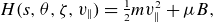 \begin{equation} H(s,\theta ,\zeta ,v_{\|})=\textstyle \frac {1}{2} mv_{\|}^2 + \mu B, \end{equation}
where $m$
is particle mass,
$m$
is particle mass, $B$
is the magnetic field magnitude,
$B$
is the magnetic field magnitude, $v_{\|}$
is the velocity of the particle parallel to the field and
$v_{\|}$
is the velocity of the particle parallel to the field and $\mu$
is the magnetic moment. For particle motion,
$\mu$
is the magnetic moment. For particle motion, $H$
is conserved and equal to total particle energy. This statement shows that
$H$
is conserved and equal to total particle energy. This statement shows that $\mu B$
acts as an effective potential for a particle in a magnetic field. An illustration of this effective potential energy attribute is shown in figure 1. For quasisymmetric configurations, field strength is a function of the helical angle
$\mu B$
acts as an effective potential for a particle in a magnetic field. An illustration of this effective potential energy attribute is shown in figure 1. For quasisymmetric configurations, field strength is a function of the helical angle $\chi =\theta -N\zeta$
for poloidal Boozer coordinate
$\chi =\theta -N\zeta$
for poloidal Boozer coordinate $\theta$
, toroidal Boozer angle
$\theta$
, toroidal Boozer angle $\zeta$
and helicity
$\zeta$
and helicity $N$
, which takes on value
$N$
, which takes on value $0$
for QA configurations and
$0$
for QA configurations and $\pm N_{fp}$
for QH configurations, where
$\pm N_{fp}$
for QH configurations, where $N_{fp}$
is the number of field periods. The helical angle
$N_{fp}$
is the number of field periods. The helical angle $\chi$
is defined such that for quasisymmetric configurations,
$\chi$
is defined such that for quasisymmetric configurations, $B(s,\chi$
), where
$B(s,\chi$
), where $s$
is the normalized flux. As a particle encounters varying
$s$
is the normalized flux. As a particle encounters varying $B$
throughout its orbit,
$B$
throughout its orbit, $B_{\text{crit}}$
is the field strength value at which a particle will bounce. The value of pitch angle
$B_{\text{crit}}$
is the field strength value at which a particle will bounce. The value of pitch angle $\lambda =\mu B_0/H$
, where
$\lambda =\mu B_0/H$
, where $B_0$
is the normalizing field strength on-axis, will determine the effective potential and the value of
$B_0$
is the normalizing field strength on-axis, will determine the effective potential and the value of $B_{\text{crit}}$
.
$B_{\text{crit}}$
.
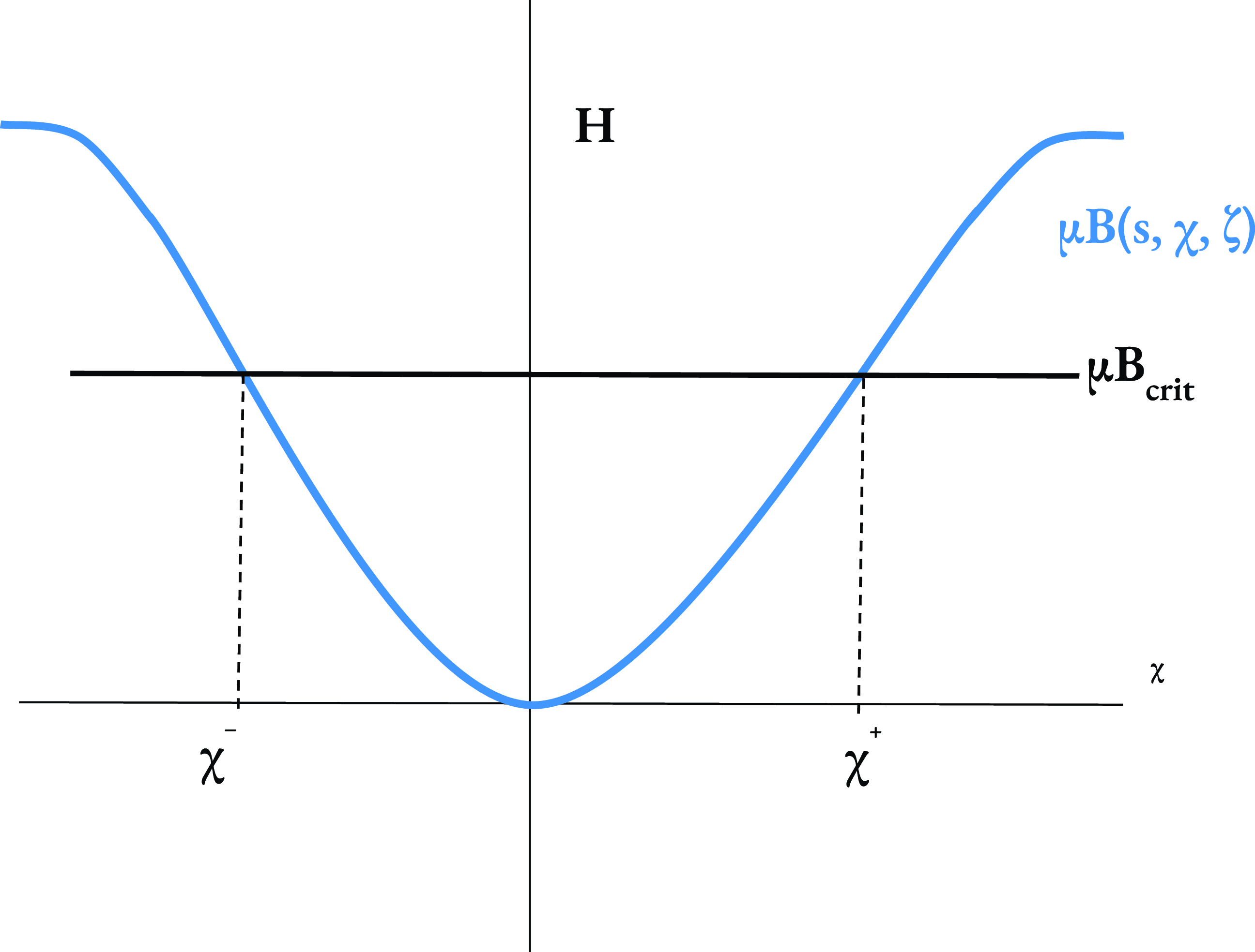
Figure 1. The effective potential at constant $s$
determined by
$s$
determined by $\mu B$
. Here,
$\mu B$
. Here, $\chi _{-}$
and
$\chi _{-}$
and $\chi _+$
are the mirror points along the
$\chi _+$
are the mirror points along the $\chi$
axis, and
$\chi$
axis, and $\mu B_{\text{crit}}$
the total energy for the particle.
$\mu B_{\text{crit}}$
the total energy for the particle.
3. Equilibria
We perform our analysis on reactor-scale configurations with finite- $\beta$
for
$\beta$
for $\beta = ({2\mu _0\langle p \rangle }/{B^2})$
, where
$\beta = ({2\mu _0\langle p \rangle }/{B^2})$
, where $\langle p \rangle$
is the mean plasma pressure and
$\langle p \rangle$
is the mean plasma pressure and $\mu _0$
is the vacuum magnetic permeability constant. We use QA and QH configurations with
$\mu _0$
is the vacuum magnetic permeability constant. We use QA and QH configurations with $\beta =2.5\,\%$
(Landreman, Buller & Drevlak Reference Landreman, Buller and Drevlak2022). These equilibria were produced with VMEC (Hirshman & Whitson Reference Hirshman and Whitson1983), and therefore have no magnetic islands. Distance from quasisymmetry for these configurations can be evaluated by summing the symmetry-breaking Fourier modes (Landreman & Paul Reference Landreman and Paul2022)
$\beta =2.5\,\%$
(Landreman, Buller & Drevlak Reference Landreman, Buller and Drevlak2022). These equilibria were produced with VMEC (Hirshman & Whitson Reference Hirshman and Whitson1983), and therefore have no magnetic islands. Distance from quasisymmetry for these configurations can be evaluated by summing the symmetry-breaking Fourier modes (Landreman & Paul Reference Landreman and Paul2022)
 \begin{equation} f_{\textrm{QS}}=\mathop{{\sum }}\limits_{m, n\neq Nm/N_{fp}}\left (\frac {B_{m,n}}{B_{0,0}}\right )^2 ,\end{equation}
for integers $n, m$
. Field strength is defined such that
$n, m$
. Field strength is defined such that
 \begin{equation} B(s,\theta ,\zeta )=\mathop{{\sum }}\limits_{m,n}B_{m,n}(s)\cos {(m\theta -nN_{fp}\zeta )}. \end{equation}
The quasisymmetry metrics for these configurations are shown in figure 2. Despite both finite- $\beta$
equilibria possessing similar
$\beta$
equilibria possessing similar $f_{\textrm{QS}}$
magnitudes, we demonstrate in later sections that resonances of fast particle drift frequencies and resulting perturbation-induced transport differ significantly for these configurations.
$f_{\textrm{QS}}$
magnitudes, we demonstrate in later sections that resonances of fast particle drift frequencies and resulting perturbation-induced transport differ significantly for these configurations.
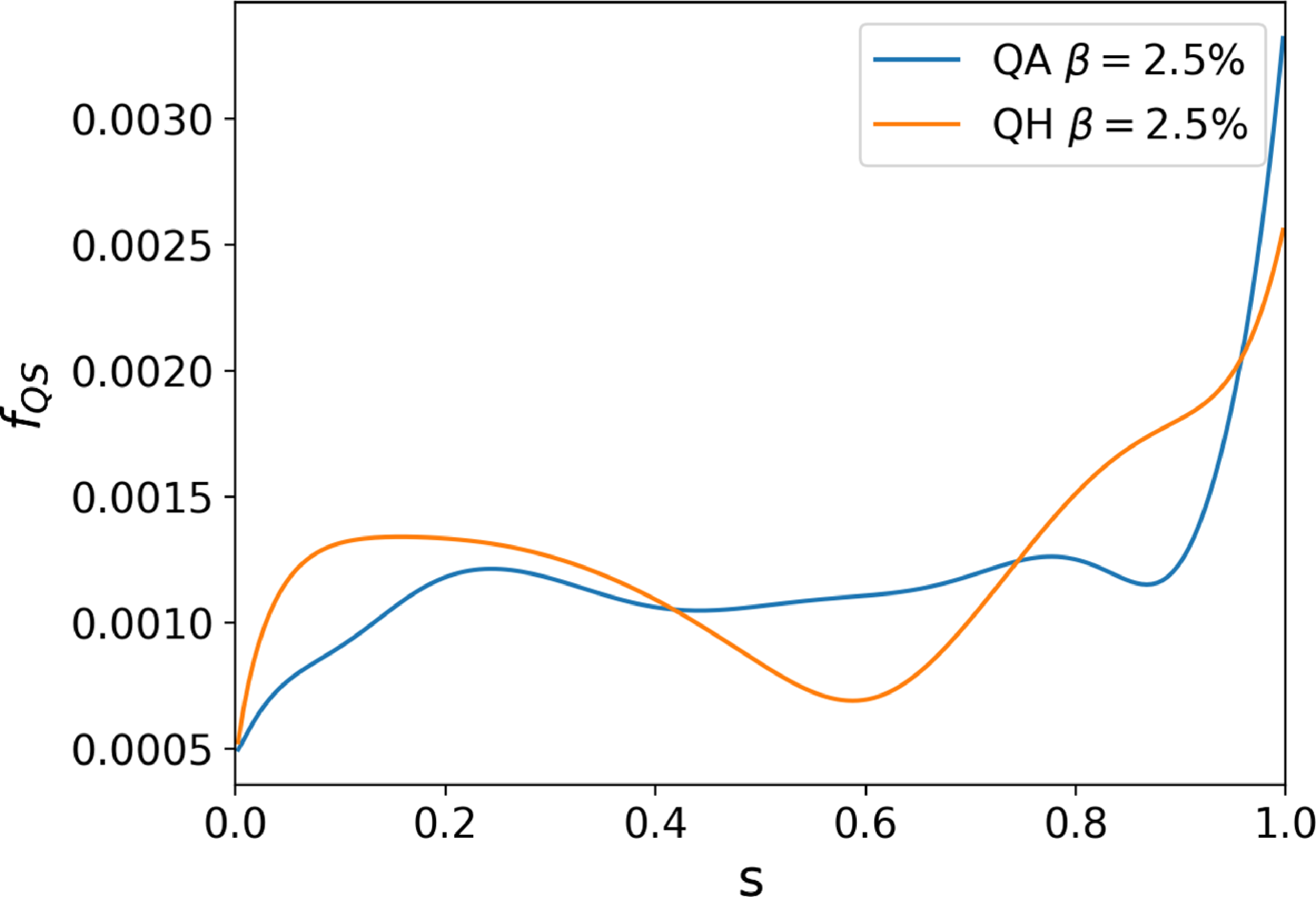
Figure 2. Quasisymmetry error $f_{\textrm{QS}}$
for VMEC equilibria used. For the two configurations with
$f_{\textrm{QS}}$
for VMEC equilibria used. For the two configurations with $\beta =2.5\,\%$
, we see similar magnitudes of
$\beta =2.5\,\%$
, we see similar magnitudes of $f_{\textrm{QS}}$
, but very different transport and resonance sensitivities will be demonstrated.
$f_{\textrm{QS}}$
, but very different transport and resonance sensitivities will be demonstrated.
4. Map computations
To visualize drift islands and guiding-center transport in these equilibria, we can construct area-preserving phase-space maps for trapped and passing particles. For a chosen pitch, each guiding-center trajectory has four dimensions: parallel velocity $v_{\|}$
, as well as three spatial dimensions in (
$v_{\|}$
, as well as three spatial dimensions in ( $s,\chi ,\zeta$
). For each particle class, this four-dimensional problem must be reduced to two dimensions for visualization. Dimension reduction depends on particle class. Energy
$s,\chi ,\zeta$
). For each particle class, this four-dimensional problem must be reduced to two dimensions for visualization. Dimension reduction depends on particle class. Energy $H$
and pitch
$H$
and pitch $\lambda$
are fixed for each trajectory. A map can be produced for each pitch value. Particles are lost when their trajectory leaves the boundary, and trajectories that travel too close to the magnetic axis are eliminated to avoid a coordinate singularity.
$\lambda$
are fixed for each trajectory. A map can be produced for each pitch value. Particles are lost when their trajectory leaves the boundary, and trajectories that travel too close to the magnetic axis are eliminated to avoid a coordinate singularity.
4.1. Passing particles
For passing particles, we define particle initial points in phase space at a chosen ( $s_0,\chi _0,v_{\|}$
) at
$s_0,\chi _0,v_{\|}$
) at $\zeta _0=0$
. We define the mapping
$\zeta _0=0$
. We define the mapping
 \begin{equation} \mathcal{M}_p(s_0,\chi _0)\longrightarrow (s',\chi ') ,\end{equation}
that advances a particle trajectory from its initial location to the resulting $(s',\chi ')$
point in the
$(s',\chi ')$
point in the $\zeta =0$
plane. Through asserting that
$\zeta =0$
plane. Through asserting that $v_{\|}$
does not change sign, we eliminate bouncing particles and use
$v_{\|}$
does not change sign, we eliminate bouncing particles and use $H$
-conservation and
$H$
-conservation and $\lambda$
to determine
$\lambda$
to determine $v_{\|}$
given
$v_{\|}$
given $(s,\chi ,\zeta )$
, enabling the two-dimensional expression of (4.1). This
$(s,\chi ,\zeta )$
, enabling the two-dimensional expression of (4.1). This $v_{\|}$
condition ensures that we capture each trajectory in unidirectional motion only, analogous to field-line flow Poincaré plots.
$v_{\|}$
condition ensures that we capture each trajectory in unidirectional motion only, analogous to field-line flow Poincaré plots.
4.2. Trapped particles
For trapped particles, $\lambda$
is chosen and particles are initialized at the bounce point where
$\lambda$
is chosen and particles are initialized at the bounce point where $B=B_{\text{crit}}=B_0/\lambda$
. Under the assumption that particles remain trapped in a single well, the mirror point in
$B=B_{\text{crit}}=B_0/\lambda$
. Under the assumption that particles remain trapped in a single well, the mirror point in $\chi$
is determined given
$\chi$
is determined given $s$
and
$s$
and $\zeta$
by seeking the value of
$\zeta$
by seeking the value of $\chi$
where
$\chi$
where $B=B_{\text{crit}}$
. The mapping is thus defined
$B=B_{\text{crit}}$
. The mapping is thus defined
 \begin{equation} \mathcal{M}_t(s_0,\zeta _0) \longrightarrow (s',\zeta '). \end{equation}
We apply (4.2) by following guiding-center trajectories until $v_{\|}$
has passed through zero for both
$v_{\|}$
has passed through zero for both $v_{\|}'\gt 0$
and
$v_{\|}'\gt 0$
and $v_{\|}'\lt 0$
, isolating a full bounce period. The second
$v_{\|}'\lt 0$
, isolating a full bounce period. The second $v_{\|}=0$
crossing corresponds to the (
$v_{\|}=0$
crossing corresponds to the ( $s,\chi ,\zeta$
) point along a trajectory where
$s,\chi ,\zeta$
) point along a trajectory where $B=B_{\text{crit}}$
, defined as
$B=B_{\text{crit}}$
, defined as $(s',\chi ',\zeta ')$
. The single-well assumption is used to further reduce dimensionality. This eliminates consideration of ripple-trapped and transitioning particles. These mirror points are then plotted in the
$(s',\chi ',\zeta ')$
. The single-well assumption is used to further reduce dimensionality. This eliminates consideration of ripple-trapped and transitioning particles. These mirror points are then plotted in the $(s,\zeta )$
-plane.
$(s,\zeta )$
-plane.
5. Characteristic frequencies
To determine the resonance conditions for both particle classes, we must first define the frequencies associated with particle motion for both trapped and passing particles. For passing particles, effective helicity is given by $\omega _{\chi }$
, the displacement in
$\omega _{\chi }$
, the displacement in $\chi$
per displacement in
$\chi$
per displacement in $\zeta$
averaged over many toroidal transits. For the mapping in (4.1)
$\zeta$
averaged over many toroidal transits. For the mapping in (4.1)
 \begin{equation} \omega _{\chi } = \frac {1}{2\pi } \left \langle \oint \dot \chi\textrm{d}t \right \rangle , \end{equation}
since passing trajectories travel a full rotation of $2\pi$
in
$2\pi$
in $\zeta$
after one map application. The average over many transits is indicated by
$\zeta$
after one map application. The average over many transits is indicated by $\langle \rangle$
and
$\langle \rangle$
and $\oint$
denotes integration over one toroidal transit. For the mapping in (4.2), trapped trajectories have toroidal precession frequency
$\oint$
denotes integration over one toroidal transit. For the mapping in (4.2), trapped trajectories have toroidal precession frequency $\omega _{\zeta }$
. This is given by the normalized change in toroidal angle
$\omega _{\zeta }$
. This is given by the normalized change in toroidal angle $\zeta$
after a full bounce period, defined as
$\zeta$
after a full bounce period, defined as
 \begin{equation} \omega _{\zeta } = \frac {1}{2\pi } \left \langle \oint \dot \zeta \textrm{d}t \right \rangle , \end{equation}
for integration over the full bounce period in $\zeta$
. The average over many bounce periods is denoted by
$\zeta$
. The average over many bounce periods is denoted by $\langle \rangle$
.
$\langle \rangle$
.
5.1. Resonances
For these characteristic frequencies, resonance conditions must be considered to evaluate relevant transport mechanisms associated with potential resonant perturbations. The resonance condition for trapped or passing particle orbits is
 \begin{equation} \omega _{\phi }=p/q ,\end{equation}
for $\omega _{\phi }=\omega _{\chi }$
or
$\omega _{\phi }=\omega _{\chi }$
or $\omega _{\zeta }$
. In other words, a particle orbit close to a resonance will nearly close on itself after
$\omega _{\zeta }$
. In other words, a particle orbit close to a resonance will nearly close on itself after $q$
map applications. When the frequency of a particle orbit meets (5.3), the orbit will be highly susceptible even to small perturbations in quasisymmetry, and is more likely to be subject to convective or diffusive losses, particularly for low-order resonances.
$q$
map applications. When the frequency of a particle orbit meets (5.3), the orbit will be highly susceptible even to small perturbations in quasisymmetry, and is more likely to be subject to convective or diffusive losses, particularly for low-order resonances.
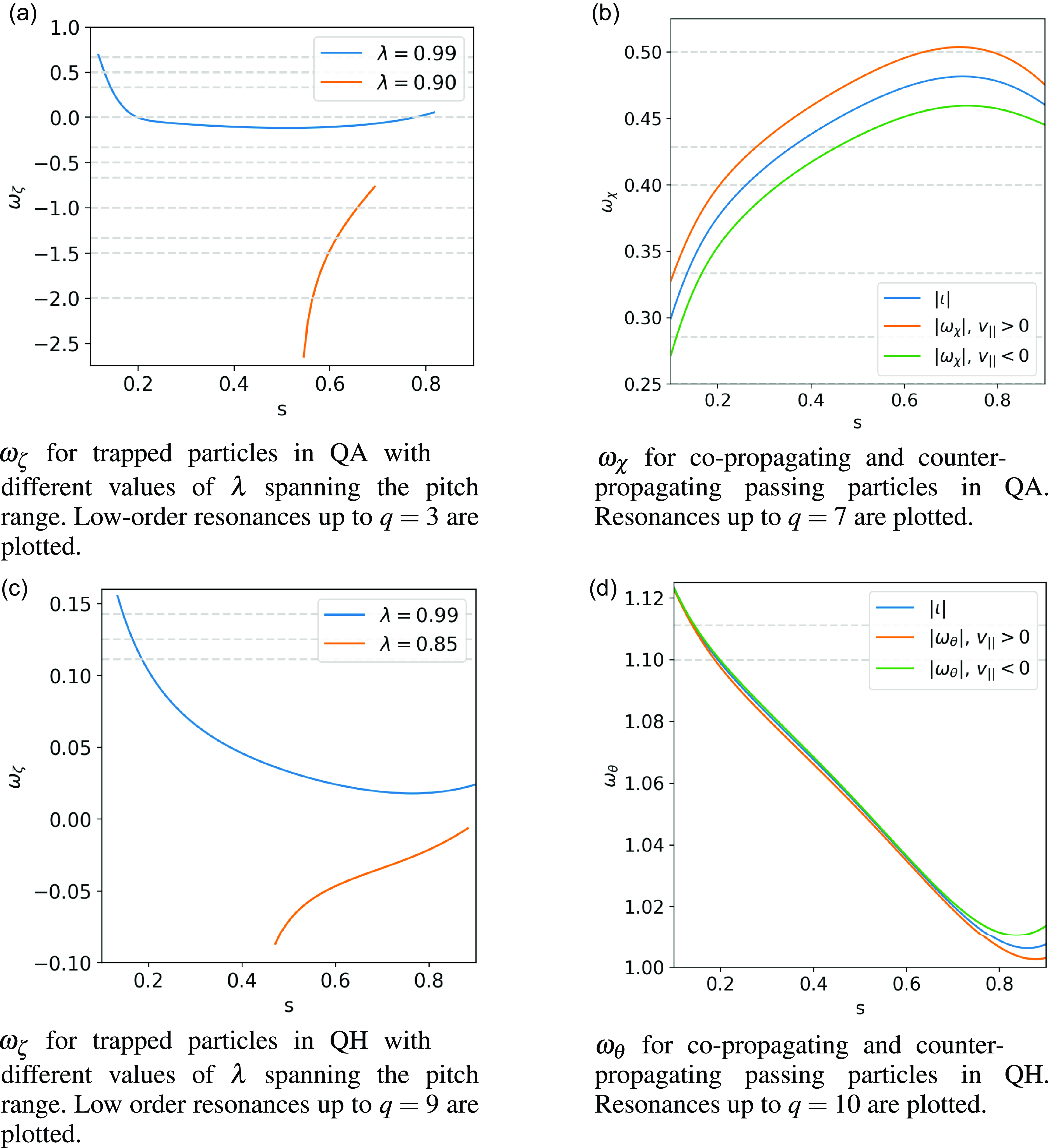
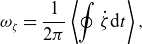
Figure 3. Frequency profiles for trapped and passing trajectories for representative values of pitch in QH $\beta =2.5\,\%$
and QA
$\beta =2.5\,\%$
and QA $\beta =2.5\,\%$
equilibria. The range of frequency profiles is determined by upper and lower bounds of the pitch range for each equilibrium. Low-order resonances are plotted as dashed gray lines for each case. For passing particles, comparison with the
$\beta =2.5\,\%$
equilibria. The range of frequency profiles is determined by upper and lower bounds of the pitch range for each equilibrium. Low-order resonances are plotted as dashed gray lines for each case. For passing particles, comparison with the $\iota$
profile is provided. For passing particles in QH,
$\iota$
profile is provided. For passing particles in QH, $\omega _{\theta }$
is shown for comparison with
$\omega _{\theta }$
is shown for comparison with $\iota$
.
$\iota$
.
Numerical results for $\omega _{\zeta }$
and
$\omega _{\zeta }$
and $\omega _{\chi }$
are shown for trapped and passing particles in QA and QH equilibria at representative values of pitch in figure 3, with low-order resonance crossings. A guiding-center tracing routine in SIMSOPT (Landreman et al. Reference Landreman, Medasani, Wechsung, Giuliani, Jorge and Zhu2021) is used for fusion-born
$\omega _{\chi }$
are shown for trapped and passing particles in QA and QH equilibria at representative values of pitch in figure 3, with low-order resonance crossings. A guiding-center tracing routine in SIMSOPT (Landreman et al. Reference Landreman, Medasani, Wechsung, Giuliani, Jorge and Zhu2021) is used for fusion-born $\alpha$
particles in the reactor-scale equilibria shown in figure 2 (Paul et al. Reference Paul, Bhattacharjee, Landreman, Alex, Velasco and Nies2022). We initialize particles at equidistant
$\alpha$
particles in the reactor-scale equilibria shown in figure 2 (Paul et al. Reference Paul, Bhattacharjee, Landreman, Alex, Velasco and Nies2022). We initialize particles at equidistant $s$
values at a constant angle
$s$
values at a constant angle $\phi =\chi$
or
$\phi =\chi$
or $\zeta$
depending on particle class. Frequencies are averaged over the guiding-center motion and symmetry-breaking modes are filtered out to isolate the frequencies of the unperturbed motion. For a perfect quasisymmetric case, the canonical momentum
$\zeta$
depending on particle class. Frequencies are averaged over the guiding-center motion and symmetry-breaking modes are filtered out to isolate the frequencies of the unperturbed motion. For a perfect quasisymmetric case, the canonical momentum $P_{\zeta }(s, \chi )$
is conserved. Since trajectories are initialized at
$P_{\zeta }(s, \chi )$
is conserved. Since trajectories are initialized at $\chi =0$
, characteristic frequencies can be expressed as functions of
$\chi =0$
, characteristic frequencies can be expressed as functions of $s$
. For trapped trajectories, profiles were produced for pitch values close to the trapped–passing boundary and the deeply trapped limit to demonstrate the range of frequency profiles present for the equilibrium. For passing trajectories, co-propagating and counter-propagating frequency profiles are shown with comparison with the rotational transform
$s$
. For trapped trajectories, profiles were produced for pitch values close to the trapped–passing boundary and the deeply trapped limit to demonstrate the range of frequency profiles present for the equilibrium. For passing trajectories, co-propagating and counter-propagating frequency profiles are shown with comparison with the rotational transform $\iota$
. At low energies in QA, we expect agreement between
$\iota$
. At low energies in QA, we expect agreement between $|\omega _{\chi }|$
and
$|\omega _{\chi }|$
and $|\iota|$
, but variation is observed since drifts enable deviation of passing trajectories from field-line flow. As a result, when optimizing for a desirable
$|\iota|$
, but variation is observed since drifts enable deviation of passing trajectories from field-line flow. As a result, when optimizing for a desirable $\iota$
, passing particle flow resonances can differ from those of the field structure. Resonant orbits in three dimensions are shown in figures 4 and 5. For passing particles, the orbit visibly closes on itself, while for trapped particles, bounce points return to the nearly the same location after
$\iota$
, passing particle flow resonances can differ from those of the field structure. Resonant orbits in three dimensions are shown in figures 4 and 5. For passing particles, the orbit visibly closes on itself, while for trapped particles, bounce points return to the nearly the same location after $q$
bounce periods.
$q$
bounce periods.
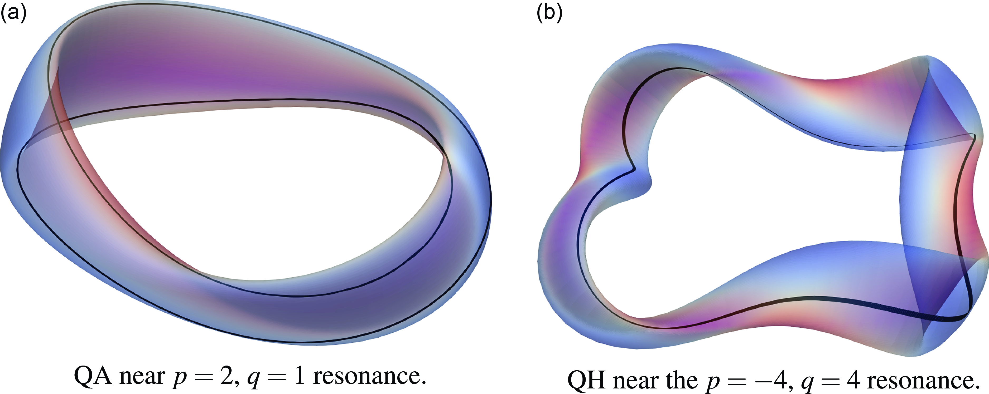
Figure 4. Passing particle trajectories close to resonance in QA and QH stellarator VMEC equilibria. Field strength on the last closed flux surface is indicated in color.
Figure 5. Trapped particle trajectories close to resonance in QA and QH stellarator VMEC equilibria. Field strength on the last closed flux surface is indicated in color. Bounce points are shown in green.
5.2. Near-axis approximation
These frequency expressions can be simplified using the near-axis approximation for the field structure. This is analogous to the large aspect-ratio tokamak assumption (Helander & Sigmar Reference Helander and Sigmar2005; Shaing, Ida & Sabbagh Reference Shaing, Ida and Sabbagh2015). In near-axis theory, the magnetic field strength to first order in the distance from the magnetic axis $r = \sqrt {2\psi /B_0}$
for flux
$r = \sqrt {2\psi /B_0}$
for flux $\psi$
is given by (Landreman & Sengupta Reference Landreman and Sengupta2018)
$\psi$
is given by (Landreman & Sengupta Reference Landreman and Sengupta2018)
 \begin{equation} B = B_0 \left [1 - r \bar \eta \cos (\chi )\right ], \end{equation}
where $\bar \eta$
is a constant. To lowest order, rotational transform is constant,
$\bar \eta$
is a constant. To lowest order, rotational transform is constant, $\iota = \iota _0$
. For a configuration with helicity
$\iota = \iota _0$
. For a configuration with helicity $N$
, the toroidal transit frequency after one full bounce period (Rodríguez & Mackenbach Reference Rodríguez and Mackenbach2023) is then proportional to
$N$
, the toroidal transit frequency after one full bounce period (Rodríguez & Mackenbach Reference Rodríguez and Mackenbach2023) is then proportional to
 \begin{equation} \omega _{\zeta }\propto \frac {1}{(\iota _0 -N)^2}\left [2E(k^2)-K(k^2)\right ], \end{equation}
where
 \begin{equation} k^2=\frac {1-\lambda +\lambda r \bar \eta }{2\lambda r \bar \eta }. \end{equation}
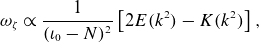
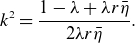
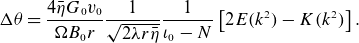
More detail is provided in Appendix A. In figure 6, (5.5) is compared with the frequency profile produced by tracing particles in a near-axis field geometry given in (5.4), indicating good agreement. Note that this near-axis field is not a VMEC equilibrium. This comparison is performed for particles at 0.1 eV, and deviation from the analytic form given by near axis occurs at higher energies. This occurs because (5.5) is produced by averaging over a field line, which exhibits agreement for small gyroradii, but gyroradius increases at higher energies. Figure 7 demonstrates the pitch for which $2E(k^2)-K(k^2)$
crosses through zero. Heightened sensitivity to the
$2E(k^2)-K(k^2)$
crosses through zero. Heightened sensitivity to the $\omega _{\zeta }=0$
crossing for trapped particles is suggested. This implies that additional care should be taken to reduce symmetry-breaking modes for trajectories that resonate with the zero crossing. The
$\omega _{\zeta }=0$
crossing for trapped particles is suggested. This implies that additional care should be taken to reduce symmetry-breaking modes for trajectories that resonate with the zero crossing. The $1/(\iota _0-N)^2$
scaling results in a larger magnitude of
$1/(\iota _0-N)^2$
scaling results in a larger magnitude of $\omega _{\zeta }$
for QA than for QH configurations, suggesting a higher shear for QA and a heightened sensitivity to the zero crossing for QH due to comparatively lower shear.
$\omega _{\zeta }$
for QA than for QH configurations, suggesting a higher shear for QA and a heightened sensitivity to the zero crossing for QH due to comparatively lower shear.
Figure 6. Comparison between the analytic form for $\omega _{\zeta }$
given by (5.5) and numerical results from guiding-center tracing for
$\omega _{\zeta }$
given by (5.5) and numerical results from guiding-center tracing for $\omega _{\zeta }$
for a near-axis field.
$\omega _{\zeta }$
for a near-axis field.
We observe the impact of the $\omega _{\zeta }=0$
crossing on particles in a QH equilibrium in figure 8. Three zero crossings result in the formation of large islands, which can lead to substantial convective radial transport. This suggests that quasisymmetry error should be reduced for pitches such that the toroidal precession frequency exhibits resonance with the zero crossing.
$\omega _{\zeta }=0$
crossing on particles in a QH equilibrium in figure 8. Three zero crossings result in the formation of large islands, which can lead to substantial convective radial transport. This suggests that quasisymmetry error should be reduced for pitches such that the toroidal precession frequency exhibits resonance with the zero crossing.
Figure 7. The value of (5.5) versus pitch. The resonance at zero is indicated by the dashed line.
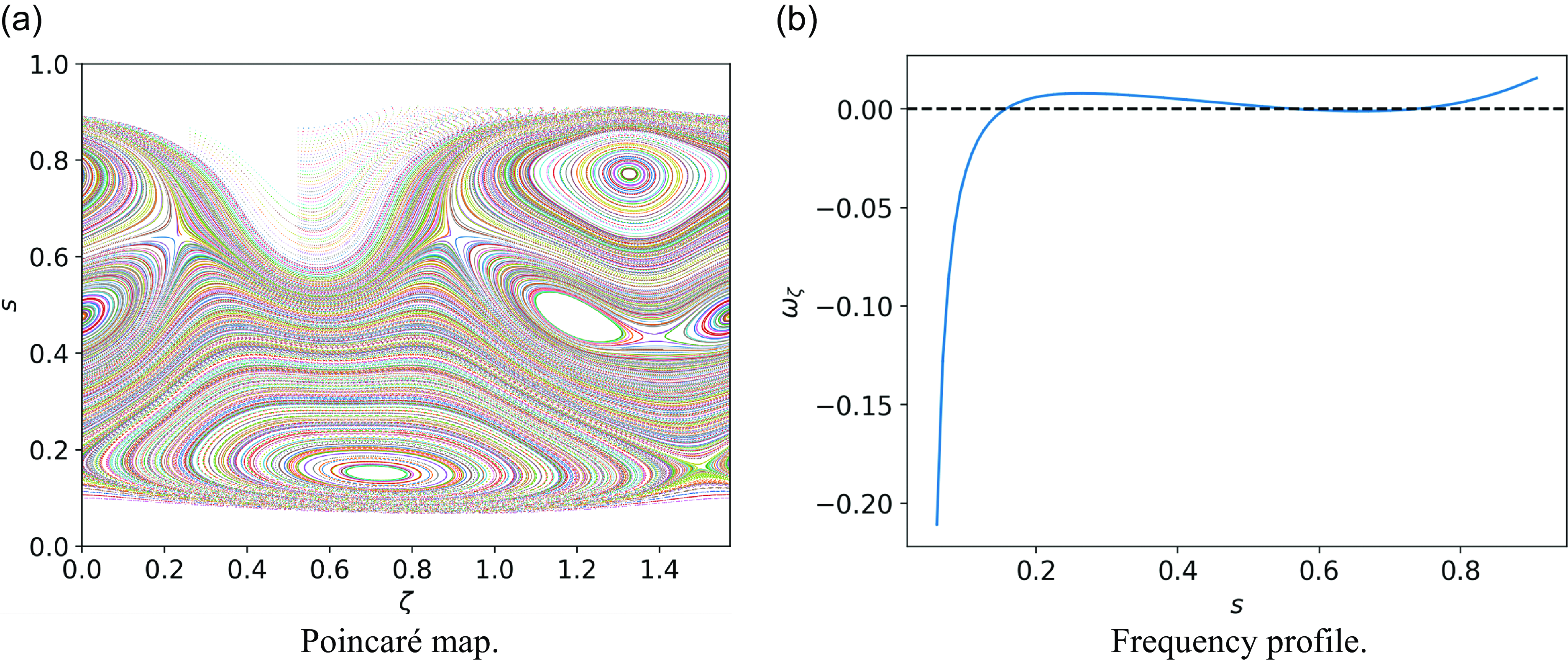
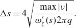
Figure 8. Poincaré map and frequency profile for trapped particles in QH equilibrium with $2.5\,\% \beta$
at
$2.5\,\% \beta$
at $\lambda =0.95$
. Multiple zero crossings in the frequency profile correspond to island structures that appear distinctly at three different radii, resulting in a definitively non-twist map structure (del Castillo-Negrete, Greene & Morrison Reference del Castillo-Negrete, Greene and Morrison1996).
$\lambda =0.95$
. Multiple zero crossings in the frequency profile correspond to island structures that appear distinctly at three different radii, resulting in a definitively non-twist map structure (del Castillo-Negrete, Greene & Morrison Reference del Castillo-Negrete, Greene and Morrison1996).
5.3. Pseudo-periodic trajectories
Once perturbations are introduced, particle orbits are likely to become non-integrable, in that their orbits no longer lie on invariant surfaces in phase space. For the non-integrable Hamiltonian system, it is useful to construct a nearby integrable Hamiltonian system, which can be used to decompose the given non-integrable Hamiltonian as an integrable Hamiltonian plus a small perturbation. Building on work by Dewar and co-workers (Dewar et al. Reference Dewar, Hudson and Price1994; Dewar & Khorev Reference Dewar and Khorev1995; Hudson & Dewar Reference Hudson and Dewar1996; Dewar, Hudson & Gibson Reference Dewar, Hudson and Gibson2012), we can construct a mapping that allows us to construct periodic orbits of the nearby integrable system. These orbits will pass through the X- and O-points of resonant perturbations, since they are stationary points of the action for this Hamiltonian system (Dewar & Khorev Reference Dewar and Khorev1995). Beginning with an initial guess for the radial location of the $p/q$
resonance at some angle
$p/q$
resonance at some angle $\phi _0$
, the map is applied
$\phi _0$
, the map is applied $q$
times. During these map applications, a root solve is performed to recover a pseudo-periodic orbit that closes in
$q$
times. During these map applications, a root solve is performed to recover a pseudo-periodic orbit that closes in $\phi$
but not in
$\phi$
but not in $s$
, arriving at
$s$
, arriving at $(s_0,\phi _0)$
. The radial difference
$(s_0,\phi _0)$
. The radial difference $\nu = s_q - s_0$
is a measure of the resonant perturbation that results in the island formation. This is performed for uniformly spaced values of
$\nu = s_q - s_0$
is a measure of the resonant perturbation that results in the island formation. This is performed for uniformly spaced values of $\phi$
. The pseudocode in Algorithm 1 describes this process, also illustrated in figure 9. Radial distance
$\phi$
. The pseudocode in Algorithm 1 describes this process, also illustrated in figure 9. Radial distance $\nu (\phi )$
is a constant along each trajectory, and varies sinusoidally across the angle coordinate. This radial difference is related to the distance from integrability and can be used to evaluate island width.
$\nu (\phi )$
is a constant along each trajectory, and varies sinusoidally across the angle coordinate. This radial difference is related to the distance from integrability and can be used to evaluate island width.
Algorithm 1 Pseudocode for the discovery of pseudo-periodic curves
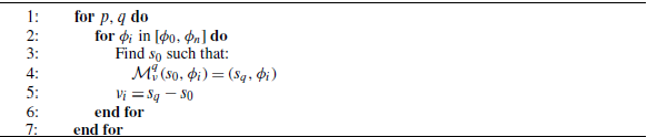
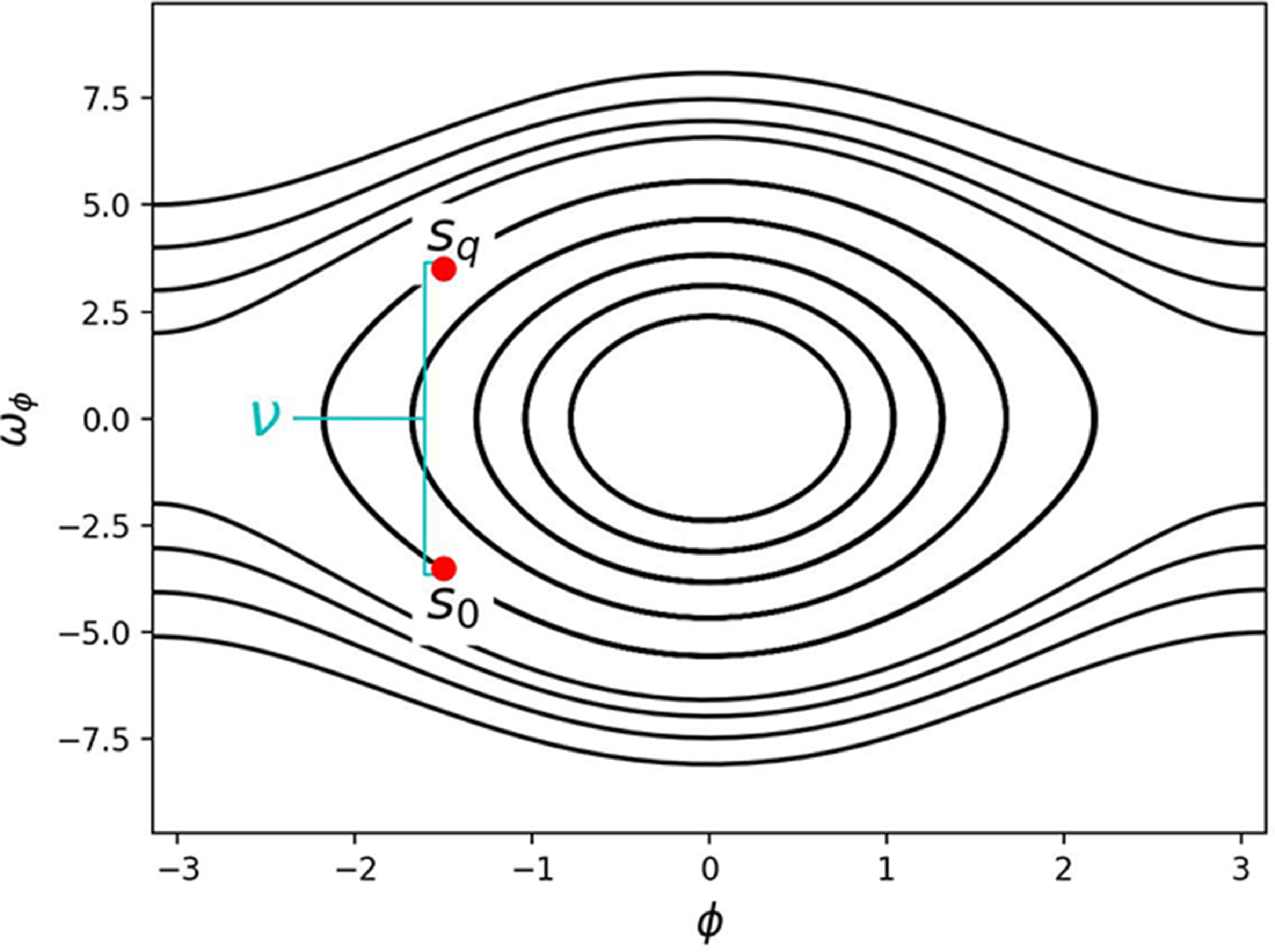
Figure 9. Schematic of the pseudo-periodic curve root solve.
For the passing map, our characteristic frequency is $\omega _{\chi }$
. For a resonance
$\omega _{\chi }$
. For a resonance $\omega _{\chi }(s) = p/q$
, the island width is
$\omega _{\chi }(s) = p/q$
, the island width is
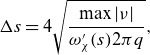 \begin{equation} \Delta s = 4 \sqrt {\frac {\max |\nu |}{\omega _{\chi }'(s) 2\pi q }}, \end{equation}
where $\max |\nu |$
refers to the maximum value of
$\max |\nu |$
refers to the maximum value of $|\nu |$
among all pseudo-orbits equally spaced in
$|\nu |$
among all pseudo-orbits equally spaced in $\phi$
at the resonance
$\phi$
at the resonance $p/q$
. For trapped particles with a resonance
$p/q$
. For trapped particles with a resonance $\omega _{\zeta }(s) = p/q$
, the island width is
$\omega _{\zeta }(s) = p/q$
, the island width is
 \begin{equation} \Delta s = 4 \sqrt {\frac {\max |\nu |}{\omega _{\zeta }'(s) 2\pi q }}. \end{equation}
The details of this derivation from the Hamiltonian in action-angle coordinates is provided in Appendix A.3, and application to guiding-center motion is shown in Appendix B. Note that this derivation relies on the linearized Hamiltonian, which uses the small island assumption, and is therefore not valid for wide islands. This expression also does not take into account non-twist map topologies.
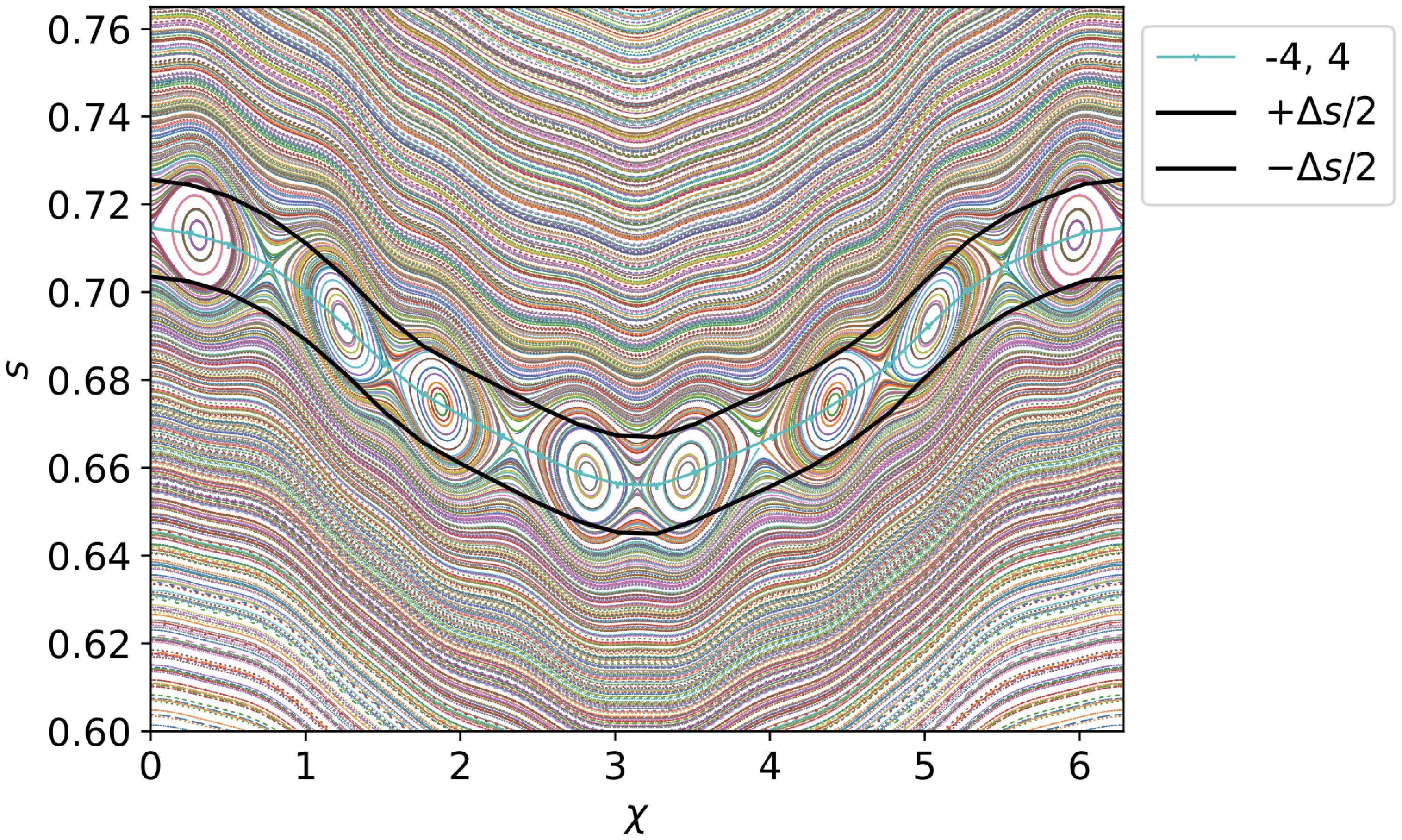
Figure 10. Comparison of theoretical island width with numerically determined result for co-propagating passing particles in QH. Theoretical island width is produced from (5.7) using the corresponding value of $\nu$
output by the pseudo-periodic curve routine.
$\nu$
output by the pseudo-periodic curve routine.
6. Results
We investigated characteristic frequencies and resonances crossings for fusion-born $\alpha$
-particles in QA and QH equilibria. For trapped trajectories in the QH
$\alpha$
-particles in QA and QH equilibria. For trapped trajectories in the QH $\beta =2.5\,\%$
case shown in figure 8, multiple zero crossings of the low-shear toroidal precession frequency profile result in three distinct island structures. The resulting non-twist map (del Castillo-Negrete et al. Reference del Castillo-Negrete, Greene and Morrison1996) caused by the low shear and non-monotonic behavior in
$\beta =2.5\,\%$
case shown in figure 8, multiple zero crossings of the low-shear toroidal precession frequency profile result in three distinct island structures. The resulting non-twist map (del Castillo-Negrete et al. Reference del Castillo-Negrete, Greene and Morrison1996) caused by the low shear and non-monotonic behavior in $\omega _{\zeta }$
is shown in figure 8(b). Multiple island chains appear at different radial locations sharing the same X-points. These perturbations demonstrate the significant impact of the zero crossing on wide island formation, supported by the analytic result presented in (5.5). The shearless curve characteristic of non-twist maps is robust to perturbations (Mugnaine et al. Reference Mugnaine, Jr, Viana, Caldas and Morrison2024), preventing stochasticity even for this wide island case. Equation (5.5) shows that QH toroidal precession frequencies will be more sensitive to the zero crossing than QA frequencies due to the inverse scaling with the square of effective helicity.
$\omega _{\zeta }$
is shown in figure 8(b). Multiple island chains appear at different radial locations sharing the same X-points. These perturbations demonstrate the significant impact of the zero crossing on wide island formation, supported by the analytic result presented in (5.5). The shearless curve characteristic of non-twist maps is robust to perturbations (Mugnaine et al. Reference Mugnaine, Jr, Viana, Caldas and Morrison2024), preventing stochasticity even for this wide island case. Equation (5.5) shows that QH toroidal precession frequencies will be more sensitive to the zero crossing than QA frequencies due to the inverse scaling with the square of effective helicity.
For passing particles, agreement with (5.7) is investigated using the QH $\beta =2.5\,\%$
map for a
$\beta =2.5\,\%$
map for a $p=-1, q=2$
island chain shown in figure 10. A set of pseudo-periodic curves is produced for the
$p=-1, q=2$
island chain shown in figure 10. A set of pseudo-periodic curves is produced for the $(p,q)=(-1,2)$
resonance, shown in figure 10. Given
$(p,q)=(-1,2)$
resonance, shown in figure 10. Given $\nu$
from the root solve, we observe favorable agreement between the resulting island width and (5.7). This island chain is the only sizeable island structure for this case. The pseudo-periodic curve defined in Algorithm1 successfully resolves the nearby integrable Hamiltonian system, passing through the X- and O-points of phase-space islands in the true map as expected. This demonstrates both the success of our pseudo-periodic curve construction and applicability of our analytic form for island width to characterize island formation.
$\nu$
from the root solve, we observe favorable agreement between the resulting island width and (5.7). This island chain is the only sizeable island structure for this case. The pseudo-periodic curve defined in Algorithm1 successfully resolves the nearby integrable Hamiltonian system, passing through the X- and O-points of phase-space islands in the true map as expected. This demonstrates both the success of our pseudo-periodic curve construction and applicability of our analytic form for island width to characterize island formation.
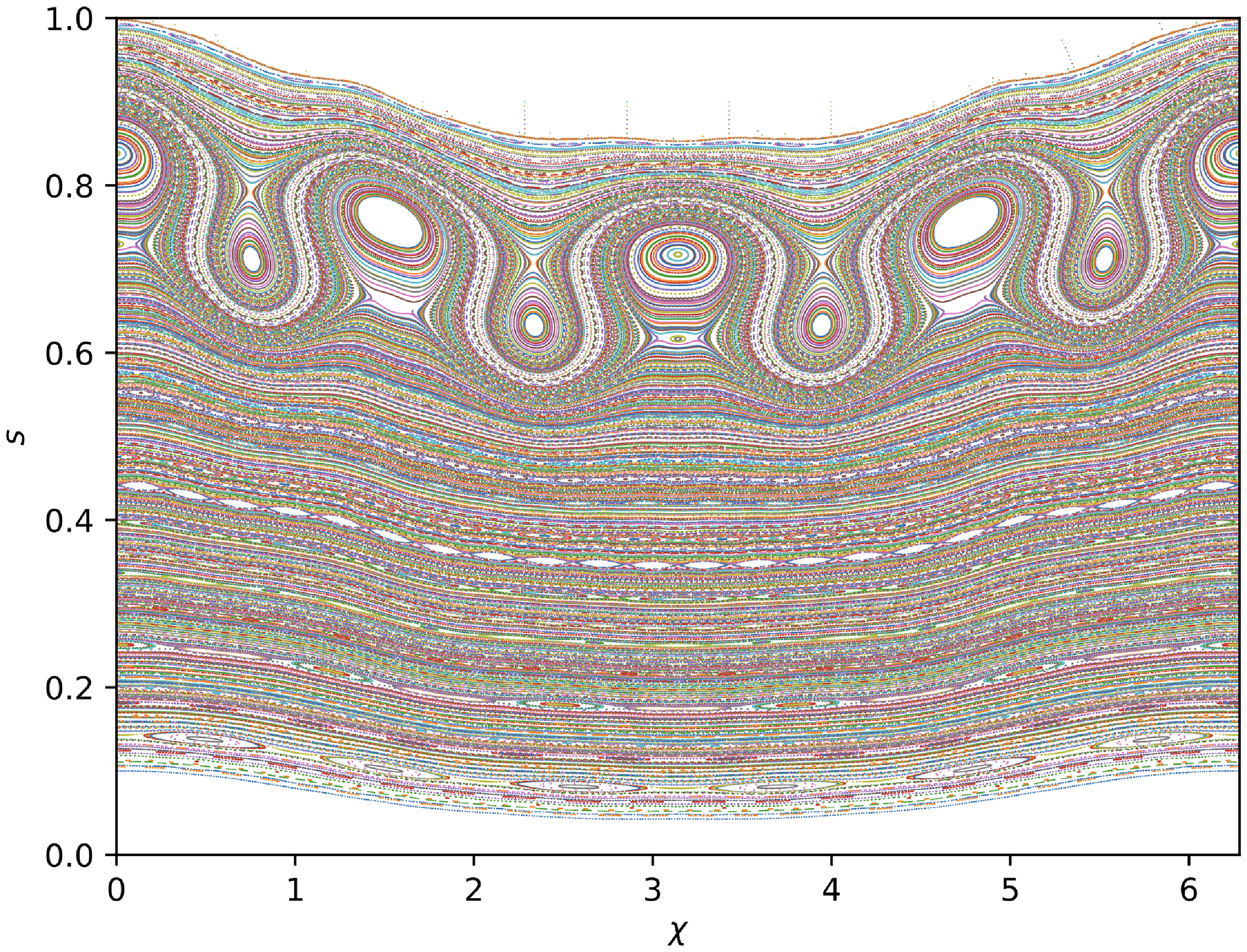
Figure 11. Poincaré map for co-propagating passing particles in QA $\beta =2.5\,\%$
. The map demonstrates a structure characteristic of low shear in the region
$\beta =2.5\,\%$
. The map demonstrates a structure characteristic of low shear in the region $0.6 \lt s \lt 0.9$
.
$0.6 \lt s \lt 0.9$
.
The Poincaré map for passing particles in QA is shown in figure 11. A distinctive non-twist map structure is again observed. The topology of this case is indicated by the main island chain oscillating in radial position, as the X- and O-points are not collinear. Frequency behavior for this case is shown in figure 3(b), with low shear in the radial range $0.6\lt s\lt 0.8$
. The pseudo-periodic curve method is not robust to cases with large regions of low shear at a resonance, since degeneracy of resonance locations inhibits the radial root solve.
$0.6\lt s\lt 0.8$
. The pseudo-periodic curve method is not robust to cases with large regions of low shear at a resonance, since degeneracy of resonance locations inhibits the radial root solve.
In contrast, the map for the trapped case in this QA equilibrium is highly stochastic, shown in figure 12(a). The pseudo-periodic curves found indicate the presence of a number of low-order resonant perturbations in this configuration, implying susceptibility to large island formation. A high level of stochasticity is observed over the full domain, indicating diffusive transport for trapped particles in this configuration. The pseudo-periodic curves are used to quantify island width for each of these low-order resonances, and these widths are used to assess island overlap for this case. In figure 12(b) we compare the phase-space map with (5.8) to determine regions of island overlap for each low-order resonance. This extensive overlap results from this QA equilibrium having higher shear, as $\omega _{\zeta }$
crosses through several lower-order resonances over a short radial distance and causes phase-space stochasticity. This suggests that minimizing the number of resonances crossed by energetic particle frequency profiles should be conducted for QA configurations. Additionally, the contribution of the perturbation from QA to the bounce-averaged radial drift over a resonant trajectory should be suppressed.
$\omega _{\zeta }$
crosses through several lower-order resonances over a short radial distance and causes phase-space stochasticity. This suggests that minimizing the number of resonances crossed by energetic particle frequency profiles should be conducted for QA configurations. Additionally, the contribution of the perturbation from QA to the bounce-averaged radial drift over a resonant trajectory should be suppressed.
Comparison between trapped and passing cases for both QA and QH reveals the difference in impact of resonances for each particle class. The map for passing trajectories in QA in figure 10 shows one significant resonance, while in contrast the trapped map in figure 12(a) demonstrates significant resonant overlap and the presence of several low-order resonances. For QH, the co-propagating passing map demonstrates a single resonance crossing with a fairly small island chain, while the trapped particle map at $\lambda =0.95$
demonstrates several large islands due to zero-crossing sensitivity. These representative cases indicate that the passing trajectories are less impacted by resonances than trapped trajectories. This is likely a result of the fact that equilibria are optimized to have few resonances for
$\lambda =0.95$
demonstrates several large islands due to zero-crossing sensitivity. These representative cases indicate that the passing trajectories are less impacted by resonances than trapped trajectories. This is likely a result of the fact that equilibria are optimized to have few resonances for $\iota$
, which is similar to
$\iota$
, which is similar to $\omega _{\chi }$
, as shown in figure 3.
$\omega _{\chi }$
, as shown in figure 3.
Figure 12. True map and set of pseudo-periodic curves for trapped particles in QA $\beta =2.5\,\%$
equilibrium, compared with island overlap for
$\beta =2.5\,\%$
equilibrium, compared with island overlap for $\lambda =0.949$
. Significant stochasticity in the trapped map is confirmed to be a result of island overlap, shown in figure 12(b) plotted with the toroidal transit frequency as a function of radius, shown in black. Island widths are computed from (5.8). The radial location of each resonance is indicated by the dashed lines, while the width is given by the band in the corresponding color. The high degree of stochasticity is indicated by the many regions of island overlap across the domain.
$\lambda =0.949$
. Significant stochasticity in the trapped map is confirmed to be a result of island overlap, shown in figure 12(b) plotted with the toroidal transit frequency as a function of radius, shown in black. Island widths are computed from (5.8). The radial location of each resonance is indicated by the dashed lines, while the width is given by the band in the corresponding color. The high degree of stochasticity is indicated by the many regions of island overlap across the domain.
7. Conclusion
With phase-space Poincaré maps and quadratic flux minimization, we use distance from integrability to characterize both diffusive and convective transport for trapped and passing guiding-center trajectories in both QA and QH equilibria with $\beta =2.5\,\%$
. We have shown that, even in cases with low quasisymmetry error and where the magnetic field is integrable, phase-space integrability is not guaranteed. Characterization of island widths and island overlap agree favorably with numerical guiding-center tracing results from SIMSOPT. We observe that the QH equilibrium had characteristic frequency profiles with lower shear than the QA equilibrium for both particle classes. Our expression for trapped particle toroidal precession frequency (5.5) using the near-axis formulation supports this result due to an inverse scaling with the square of effective helicity. The heightened sensitivity of trapped trajectories in QH to the zero crossing of the precession frequency was indicated. As a result of lower shear, QH precession frequency profiles crossed through fewer low-order resonances than QA profiles. Correspondingly, the QH trapped particle toroidal precession frequency profile exhibited multiple zero crossings and the resulting formation of large drift islands. Since this profile has low shear near zero, the zero crossing is a more significant factor in convective transport than for the QA case considered. For trapped particles in QA, while this case had no zero crossing, higher shear of the frequency profile contributed to several low-order resonance crossings, leading to wide overlapping islands forming, causing diffusive transport. Since QA equilibria tend to have higher precession frequency shear than QH equilibria, we conclude that island overlap and diffusive transport are more likely in QA than in QH equilibria. Additionally, the co-propagating passing map for finite-
$\beta =2.5\,\%$
. We have shown that, even in cases with low quasisymmetry error and where the magnetic field is integrable, phase-space integrability is not guaranteed. Characterization of island widths and island overlap agree favorably with numerical guiding-center tracing results from SIMSOPT. We observe that the QH equilibrium had characteristic frequency profiles with lower shear than the QA equilibrium for both particle classes. Our expression for trapped particle toroidal precession frequency (5.5) using the near-axis formulation supports this result due to an inverse scaling with the square of effective helicity. The heightened sensitivity of trapped trajectories in QH to the zero crossing of the precession frequency was indicated. As a result of lower shear, QH precession frequency profiles crossed through fewer low-order resonances than QA profiles. Correspondingly, the QH trapped particle toroidal precession frequency profile exhibited multiple zero crossings and the resulting formation of large drift islands. Since this profile has low shear near zero, the zero crossing is a more significant factor in convective transport than for the QA case considered. For trapped particles in QA, while this case had no zero crossing, higher shear of the frequency profile contributed to several low-order resonance crossings, leading to wide overlapping islands forming, causing diffusive transport. Since QA equilibria tend to have higher precession frequency shear than QH equilibria, we conclude that island overlap and diffusive transport are more likely in QA than in QH equilibria. Additionally, the co-propagating passing map for finite- $\beta$
QA illustrated a characteristic non-twist map, corroborated by the non-monotonic frequency profile. Overall, we found that passing particle trajectories are less subject to resonances than trapped particle trajectories. This is likely a result of the fact that optimization to minimize resonances in
$\beta$
QA illustrated a characteristic non-twist map, corroborated by the non-monotonic frequency profile. Overall, we found that passing particle trajectories are less subject to resonances than trapped particle trajectories. This is likely a result of the fact that optimization to minimize resonances in $\iota$
can help reduce resonances in passing particle frequencies, although drifts can have some impact.
$\iota$
can help reduce resonances in passing particle frequencies, although drifts can have some impact.
These methods can be used to evaluate equilibria at reactor scale. Future work could extend the pseudo-periodic curve approach to be robust to non-twist map topologies. Evaluations of distance from integrability, island width, and island overlap could be used to inform equilibrium optimization. In particular, optimization of the drift-averaged frequency profiles over a range of pitch angles can be performed to alter shear profiles favorably (Mackenbach et al. Reference Mackenbach, Duff, Gerard, Proll, Helander and Hegna2023). For example, for QA, optimization could be performed to ensure the toroidal transit frequency profiles have lower shear to reduce the number of crossings through lower-order resonances, which could prevent overlap. For QH, the range of pitch angles for which the zero crossing is present can be reduced. Optimization to reduce resonance with the zero crossing conducted for QI using $\Gamma _c$
(Velasco et al. Reference Velasco, Calvo, Sánchez and Parra2023) could be applied to QH for the same purpose. For both symmetries, careful quasisymmetry error reduction could be conducted for particles over a range of pitch angles that resonate with low-order modes, and island width can be targeted. Using
$\Gamma _c$
(Velasco et al. Reference Velasco, Calvo, Sánchez and Parra2023) could be applied to QH for the same purpose. For both symmetries, careful quasisymmetry error reduction could be conducted for particles over a range of pitch angles that resonate with low-order modes, and island width can be targeted. Using $\Gamma _c$
, trapped particle resonances with small drift precession can be targeted during optimization, but this does not address island width directly (Velasco et al. Reference Velasco, Calvo, Mulas, Sánchez, Parra and Cappa2021). By avoiding significant resonances through optimization, we expect to be less sensitive to non-quasisymmetric perturbations. This can be verified using sensitivity analysis with the shape gradient (Landreman & Paul Reference Landreman and Paul2018) and Hessian matrix methods (Zhu et al. Reference Zhu, Gates, Hudson, Liu, Xu, Shimizu and Okamura2019).
$\Gamma _c$
, trapped particle resonances with small drift precession can be targeted during optimization, but this does not address island width directly (Velasco et al. Reference Velasco, Calvo, Mulas, Sánchez, Parra and Cappa2021). By avoiding significant resonances through optimization, we expect to be less sensitive to non-quasisymmetric perturbations. This can be verified using sensitivity analysis with the shape gradient (Landreman & Paul Reference Landreman and Paul2018) and Hessian matrix methods (Zhu et al. Reference Zhu, Gates, Hudson, Liu, Xu, Shimizu and Okamura2019).
There are many possible extensions of these methods. The non-conservation of the second adiabatic invariant, $J_{\|}$
, can be shown to be correlated to stochastic loss mechanisms (Paul et al. Reference Paul, Bhattacharjee, Landreman, Alex, Velasco and Nies2022; Albert et al. Reference Albert, Rath, Babin, Buchholz, Kasilov and Kernbichler2022). Non-conservation of
$J_{\|}$
, can be shown to be correlated to stochastic loss mechanisms (Paul et al. Reference Paul, Bhattacharjee, Landreman, Alex, Velasco and Nies2022; Albert et al. Reference Albert, Rath, Babin, Buchholz, Kasilov and Kernbichler2022). Non-conservation of $J_{\|}$
could be investigated for cases with island overlap (Albert et al. Reference Albert, Buchholz, Kasilov, Kernbichler and Rath2023). The QFM method could also be applied to configurations further from quasisymmetry like NCSX and ARIES-CS (Isaev et al. Reference Isaev, Mikhailov, Monticello, Mynick, Subbotin, Ku and Reiman1999; Ku et al. Reference Ku, Garabedian, Lyon, Turnbull, Grossman, Mau and Zarnstorff2008). The pseudo-periodic curve routine fails for these equilibria further from quasisymmetry, so additional work can adapt these methods for cases with more quasisymmetry error. In addition, these methods could be adapted to investigate the impact of resonances on QI and quasi-poloidal configurations.
$J_{\|}$
could be investigated for cases with island overlap (Albert et al. Reference Albert, Buchholz, Kasilov, Kernbichler and Rath2023). The QFM method could also be applied to configurations further from quasisymmetry like NCSX and ARIES-CS (Isaev et al. Reference Isaev, Mikhailov, Monticello, Mynick, Subbotin, Ku and Reiman1999; Ku et al. Reference Ku, Garabedian, Lyon, Turnbull, Grossman, Mau and Zarnstorff2008). The pseudo-periodic curve routine fails for these equilibria further from quasisymmetry, so additional work can adapt these methods for cases with more quasisymmetry error. In addition, these methods could be adapted to investigate the impact of resonances on QI and quasi-poloidal configurations.
Acknowledgements
We acknowledge funding through the U. S. Department of Energy, under contract No. DE-SC0024630 and through the Simons Foundation collaboration ‘Hidden Symmetries and Fusion Energy,’ Grant No. 601958. This research used resources of the National Energy Research Scientific Computing Center (NERSC), a Department of Energy Office of Science User Facility using NERSC award FES-ERCAP30322.
This material is based upon work supported by the U.S. Department of Energy, Office of Science, Office of Advanced Scientific Computing Research, Department of Energy Computational Science Graduate Fellowship under Award Number DE-SC0024386. This report was prepared as an account of work sponsored by an agency of the United States Government. Neither the United States Government nor any agency thereof, nor any of their employees, makes any warranty, express or implied, or assumes any legal liability or responsibility for the accuracy, completeness or usefulness of any information, apparatus, product or process disclosed, or represents that its use would not infringe privately owned rights. Reference herein to any specific commercial product, process, or service by trade name, trademark, manufacturer or otherwise does not necessarily constitute or imply its endorsement, recommendation, or favoring by the United States Government or any agency thereof. The views and opinions of authors expressed herein do not necessarily state or reflect those of the United States Government or any agency thereof.
Editor Peter Catto thanks the referees for their advice in evaluating this article.
Declaration of interests
The authors report no conflict of interest.
Appendix A. Characteristic frequency derivations
A.1 Near-axis model overview
The near-axis expansion can be used to provide an analytic form for the magnetic field from which we can produce an expression for trapped particle frequencies. This can provide insight into the behavior of trapped particles and their sensitivity to resonances. In the near-axis expansion, the magnetic field strength to first order in the distance from the magnetic axis $r = \sqrt {2\psi /B_0}$
is given by (Jorge, Sengupta & Landreman Reference Jorge, Sengupta and Landreman2020)
$r = \sqrt {2\psi /B_0}$
is given by (Jorge, Sengupta & Landreman Reference Jorge, Sengupta and Landreman2020)
 \begin{align} B = B_0 (1 - r \bar \eta \cos (\chi )), \end{align}
where $\chi = \theta - N \zeta$
is the angle such that
$\chi = \theta - N \zeta$
is the angle such that $B(r,\chi )$
,
$B(r,\chi )$
, $N$
is an integer which denotes the symmetry helicity, and
$N$
is an integer which denotes the symmetry helicity, and $B_0$
and
$B_0$
and $\bar \eta$
are constants representing field strength on-axis and field strength variation, respectively. The Boozer covariant components and rotational transform are approximated as
$\bar \eta$
are constants representing field strength on-axis and field strength variation, respectively. The Boozer covariant components and rotational transform are approximated as
 \begin{align} G(r) &= G_0 + \mathcal{O}(r^2) ,\end{align}
 \begin{align} I(r) &= I_2 r^2 + \mathcal{O}(r^4) ,\end{align}
 \begin{align} \iota (r) &= \iota _0 + \mathcal{O}(r^2) ,\end{align}
such that the field can be written as $\boldsymbol{B}=I(r)\nabla \theta + G(r)\nabla \zeta$
.
$\boldsymbol{B}=I(r)\nabla \theta + G(r)\nabla \zeta$
.
A.2 Characteristic frequencies
To gain further insight into the sensitivity of trapped particles to different resonances, it is useful to develop an analytic expression for trapped particle precession frequency $\omega _{\zeta }$
. Between bounce points, we average the precession over lowest-order motion along the field line in
$\omega _{\zeta }$
. Between bounce points, we average the precession over lowest-order motion along the field line in $\rho _*$
, so
$\rho _*$
, so $\alpha =\theta -\iota \zeta$
is fixed to be constant over a trajectory. The precession frequency can then be related to change in poloidal angle by
$\alpha =\theta -\iota \zeta$
is fixed to be constant over a trajectory. The precession frequency can then be related to change in poloidal angle by
 \begin{equation} \omega _{\zeta }=-\frac {1}{2\pi (\iota _0-N)} \Delta \theta . \end{equation}
For drift velocity $\boldsymbol{v}_d$
and unit field vector
$\boldsymbol{v}_d$
and unit field vector $\hat {\boldsymbol{b}}=\boldsymbol{B}/B$
, the change in poloidal angle during one toroidal transit is
$\hat {\boldsymbol{b}}=\boldsymbol{B}/B$
, the change in poloidal angle during one toroidal transit is
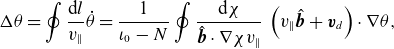 \begin{equation} \Delta \theta = \oint \frac {\textrm{d}l}{v_{\|}}\dot {\theta } = \frac {1}{\iota _0-N}\oint \frac {\textrm{d}\chi }{\hat {\boldsymbol{b}} \cdot \nabla \chi v_{\|}} \, \left (v_{\|} \hat {\boldsymbol{b}} + \boldsymbol{v}_d\right ) \cdot \nabla \theta ,\end{equation}
for integration performed in $\chi$
over a full bounce period. We can express
$\chi$
over a full bounce period. We can express $v_{\|}$
in terms of
$v_{\|}$
in terms of $B$
using the pitch angle
$B$
using the pitch angle $\lambda$
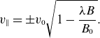 \begin{align*} v_{\|}&=\pm v_0 \sqrt {1-\frac {\lambda B}{B_0}}. \end{align*}
Using the contravariant form $\boldsymbol{B}=\nabla \psi \times \nabla \theta -\iota (\psi )\nabla \psi \times \nabla \zeta$
in (A.6) gives
$\boldsymbol{B}=\nabla \psi \times \nabla \theta -\iota (\psi )\nabla \psi \times \nabla \zeta$
in (A.6) gives
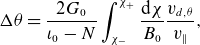 \begin{align} \Delta \theta &=\frac {2G_0}{\iota _0-N}\int _{\chi _-}^{\chi _+} \frac {\textrm{d}\chi }{B_0}\frac {v_{d,\theta }}{v_{\|}} ,\end{align}
for integration between bounce points $\chi _-$
and
$\chi _-$
and $\chi _+$
, since the sign of
$\chi _+$
, since the sign of $v_{\|}$
changes depending on bounce direction, and the
$v_{\|}$
changes depending on bounce direction, and the $\hat {\boldsymbol{b}}\cdot \nabla \theta$
term integrates to zero. We can determine
$\hat {\boldsymbol{b}}\cdot \nabla \theta$
term integrates to zero. We can determine $v_{d,\theta }$
, the poloidal component of drift velocity, in the following way:
$v_{d,\theta }$
, the poloidal component of drift velocity, in the following way:
 \begin{align*} \boldsymbol{v}_d\cdot \nabla \theta &= \frac {\left (v_0^2+v_{\|}^2\right )}{2\Omega B^2} \left (\boldsymbol{B}\times \nabla B\right )\cdot \nabla \theta = \frac {-\bar \eta \left (v_0^2+v_{\|}^2\right )}{2\Omega r }\cos {\chi } ,\end{align*}
for $\Omega =qB_0/m$
, the gyrofrequency. Substituting (A.8) into (A.7)
$\Omega =qB_0/m$
, the gyrofrequency. Substituting (A.8) into (A.7)
 \begin{align} \Delta \theta &= \frac {-\bar \eta G_0 v_0}{\Omega B_0 r}\frac {1}{\iota -N}\left [\int _{\chi _-}^{\chi _+} \textrm{d}\chi \frac {\cos {\chi }}{\sqrt {1-\lambda +\lambda r \bar \eta }}+\int _{\chi _-}^{\chi _+} \textrm{d}\chi \cos {\chi }\sqrt {1-\lambda +\lambda r \bar \eta }\right ]. \end{align}
Through re-expression in terms of $k$
from (5.6), it becomes apparent that the second term is higher order in
$k$
from (5.6), it becomes apparent that the second term is higher order in $r$
. By bounce-point symmetry, to first order we have
$r$
. By bounce-point symmetry, to first order we have
 \begin{align} \Delta \theta &= \frac {2\bar \eta G_0 v_0}{\Omega B_0 r}\frac {1}{\sqrt {2\lambda r \bar \eta }}\frac {1}{\iota _0 -N}\int _{0}^{\chi _+} d\chi \frac {2\sin ^2{\frac {\chi }{2}}-1}{\sqrt {k^2-\sin ^2{\frac {\chi }{2}}}}, \end{align}
for
 \begin{equation} k^2=\frac {1-\lambda +\lambda r \bar \eta }{2\lambda r \bar \eta }. \end{equation}
Using the variable substitution $\phi ={\chi }/{2}$
, followed by letting
$\phi ={\chi }/{2}$
, followed by letting $\sin \phi =k\sin x$
and integrating over
$\sin \phi =k\sin x$
and integrating over $x$
gives us our final expression for poloidal displacement
$x$
gives us our final expression for poloidal displacement
 \begin{align} \Delta \theta &=\frac {4\bar \eta G_0 v_0}{\Omega B_0 r}\frac {1}{\sqrt {2\lambda r \bar \eta }}\frac {1}{\iota _0 -N}\left [2E(k^2)-K(k^2)\right ]. \end{align}
Here, $K(k^2)$
and
$K(k^2)$
and $E(k^2)$
are elliptic integrals of the first and second kinds, respectively. Using (A.5), we then have toroidal displacement
$E(k^2)$
are elliptic integrals of the first and second kinds, respectively. Using (A.5), we then have toroidal displacement
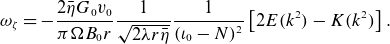 \begin{equation} \omega _{\zeta } =-\frac {2\bar \eta G_0 v_0}{\pi \Omega B_0 r}\frac {1}{\sqrt {2\lambda r \bar \eta }}\frac {1}{(\iota _0 -N)^2}\left [2E(k^2)-K(k^2)\right ]. \end{equation}
A.3 Island width in Hamiltonian systems
In order to obtain expressions for island width in general action-angle coordinates for guiding-center motion, we will make use of Hamiltonian formalism. This can be achieved if we treat the mapping integration angle $\rho$
as a time-like coordinate. For trapped particles,
$\rho$
as a time-like coordinate. For trapped particles, $\Delta \rho = 2\pi$
is the change in bounce angle after a bounce period, while for passing particles
$\Delta \rho = 2\pi$
is the change in bounce angle after a bounce period, while for passing particles $\Delta \rho =2\pi$
is the change in
$\Delta \rho =2\pi$
is the change in $\zeta$
after a toroidal transit. We can then define the linear increase in canonical angle
$\zeta$
after a toroidal transit. We can then define the linear increase in canonical angle $\overline {\phi }=\omega _{\phi } \rho$
for
$\overline {\phi }=\omega _{\phi } \rho$
for $\phi =\{\chi ,\zeta \}$
in terms of characteristic frequencies
$\phi =\{\chi ,\zeta \}$
in terms of characteristic frequencies $\omega _{\phi }=\{\omega _{\chi },\omega _{\zeta }\}$
from (5.1) and (5.2) (Lichtenberg & Lieberman Reference Lichtenberg and Lieberman1983). This can be used to develop an expression for drift island width. Consider a general one-dimensional Hamiltonian in action-angle coordinates
$\omega _{\phi }=\{\omega _{\chi },\omega _{\zeta }\}$
from (5.1) and (5.2) (Lichtenberg & Lieberman Reference Lichtenberg and Lieberman1983). This can be used to develop an expression for drift island width. Consider a general one-dimensional Hamiltonian in action-angle coordinates $(J,\overline {\phi })$
, where the unperturbed Hamiltonian reads
$(J,\overline {\phi })$
, where the unperturbed Hamiltonian reads $H_0(J)$
. The unperturbed frequency is defined by
$H_0(J)$
. The unperturbed frequency is defined by $\omega _{\phi } = \partial H_0(J)/\partial J$
. The perturbed Hamiltonian is then expressed in the action-angle coordinates of the unperturbed Hamiltonian as (Lichtenberg & Lieberman Reference Lichtenberg and Lieberman1983)
$\omega _{\phi } = \partial H_0(J)/\partial J$
. The perturbed Hamiltonian is then expressed in the action-angle coordinates of the unperturbed Hamiltonian as (Lichtenberg & Lieberman Reference Lichtenberg and Lieberman1983)
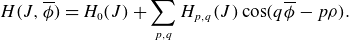 \begin{align} H(J,\overline {\phi }) = H_0(J) + \sum _{p,q} H_{p,q}(J) \cos (q\overline {\phi } - p \rho ). \end{align}
A resonance will occur if the following condition is satisfied:
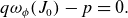 \begin{align} q \omega _{\phi }(J_0) - p = 0. \end{align}
Assume that $J_0$
satisfies such a resonance condition. We can consider the transformed coordinates,
$J_0$
satisfies such a resonance condition. We can consider the transformed coordinates, $\Phi = \overline {\phi } - \omega _{\phi }(J_0)t$
, for which the equations of motion read
$\Phi = \overline {\phi } - \omega _{\phi }(J_0)t$
, for which the equations of motion read
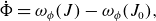 \begin{align} \dot {\Phi } &= \omega _{\phi }(J) - \omega _{\phi }(J_0), \end{align}
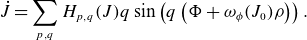 \begin{align} \dot {J} &= \sum _{p,q} H_{p,q}(J) q \sin \left ( q \left (\Phi + \omega _{\phi }(J_0) \rho \right )\right ). \end{align}
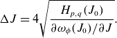
For such a resonance, the island width in the $J$
action can then be evaluated as (Lichtenberg & Lieberman Reference Lichtenberg and Lieberman1983)
$J$
action can then be evaluated as (Lichtenberg & Lieberman Reference Lichtenberg and Lieberman1983)
 \begin{align} \Delta J = 4\sqrt {\frac {H_{p,q}(J_0)}{\partial \omega _{\phi }(J_0)/\partial J}}. \end{align}
In the computation of $\omega _{\phi }$
, trajectories are initialized at the intersection of
$\omega _{\phi }$
, trajectories are initialized at the intersection of $J$
with constant
$J$
with constant $\phi$
, enabling a one-to-one mapping from
$\phi$
, enabling a one-to-one mapping from $(J,\overline {\phi }) \rightarrow (s, \phi )$
.
$(J,\overline {\phi }) \rightarrow (s, \phi )$
.
Appendix B. Poincaré map from Hamiltonian
We can adapt the island width calculation in action-angle coordinates provided in Appendix A.3 to the Poincaré maps we develop for this problem for island width analysis. In order to visualize the resonances in our system, we can make use of Poincaré maps defined for the different particle classes. In action-angle coordinates for the $n$
th mapping, the Poincaré map is defined as
$n$
th mapping, the Poincaré map is defined as $M(J^n,\overline {\phi }^n) \rightarrow (J^{n+1},\overline {\phi }^{n+1})$
. In the integrable case
$M(J^n,\overline {\phi }^n) \rightarrow (J^{n+1},\overline {\phi }^{n+1})$
. In the integrable case
 \begin{align} J^{n+1} &= J^n ,\end{align}
 \begin{align} \overline {\phi }^{n+1} &= \overline {\phi }^n + \Omega _{\rho }(J^{n+1}), \end{align}
where action-angle displacement $\Omega _{\rho }(J^{n+1}) = \omega _{\phi }(J^{n+1}) \Delta \rho$
. Here,
$\Omega _{\rho }(J^{n+1}) = \omega _{\phi }(J^{n+1}) \Delta \rho$
. Here, $\omega _{\phi }(J^{n+1})$
is the unperturbed frequency and
$\omega _{\phi }(J^{n+1})$
is the unperturbed frequency and $\Delta \rho$
is the displacement in
$\Delta \rho$
is the displacement in $\rho$
between successive mappings for integration angle
$\rho$
between successive mappings for integration angle $\rho$
. For the resonance condition (A.14), the orbit will close after
$\rho$
. For the resonance condition (A.14), the orbit will close after $q$
applications of the map. In the near-integrable case, the twist mapping will be perturbed
$q$
applications of the map. In the near-integrable case, the twist mapping will be perturbed
 \begin{align} J^{n+q} &= J^n + f(J^{n+q},\overline {\phi }^n), \end{align}
 \begin{align} \overline {\phi }^{n+q} &= \overline {\phi }^n + q\Omega _{\rho }(J^{n+q}) + g(J^{n+q},\overline {\phi }^n), \end{align}
for some periodic functions $f$
and
$f$
and $g$
. In the pseudo-periodic curve construction, we seek orbits that close in angle, so
$g$
. In the pseudo-periodic curve construction, we seek orbits that close in angle, so $g = 0$
and
$g = 0$
and $f$
only depends on
$f$
only depends on $\overline {\phi }$
and can be computed from the linearized Hamiltonian. After
$\overline {\phi }$
and can be computed from the linearized Hamiltonian. After $q$
map applications
$q$
map applications
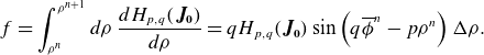 \begin{align*} f &=\int _{\rho ^n}^{\rho ^{n+1}} d\rho \, \frac {dH_{p,q}(\boldsymbol{J_0})}{d\rho } = qH_{p,q}(\boldsymbol{J_0}) \sin \left (q\overline {\phi }^n-p\rho ^n\right )\Delta \rho . \end{align*}
The distance between the periodic curve and the pseudo-periodic curve is quantified by the parameter $\nu = - f(J^{n+q},\overline {\phi }^n)$
, as discussed in § 5.3. We can then use
$\nu = - f(J^{n+q},\overline {\phi }^n)$
, as discussed in § 5.3. We can then use $\nu$
to quantify island width in the following way:
$\nu$
to quantify island width in the following way:
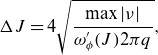 \begin{align*} \Delta J = 4 \sqrt {\frac {\max |\nu |}{\omega _{\phi }'(J) 2\pi q }}, \end{align*}
where max $|\nu |$
is the maximum value of
$|\nu |$
is the maximum value of $f$
taken over all trajectories in
$f$
taken over all trajectories in $\overline {\phi }$
. Since we initialize all particles at a constant angle
$\overline {\phi }$
. Since we initialize all particles at a constant angle $\overline {\phi }$
,
$\overline {\phi }$
, $J$
can be approximated as the flux function
$J$
can be approximated as the flux function $s$
. For the passing map analysis,
$s$
. For the passing map analysis, $\omega _{\phi } \rightarrow \omega _{\chi }$
.
$\omega _{\phi } \rightarrow \omega _{\chi }$
.


 Open access