


1. Introduction
In tokamak plasmas, the evolution of plasma currents produces time-varying electromagnetic fields that induce eddy currents within the surrounding conductors such as vacuum vessels (VV). If a sufficiently conductive shell is placed around the plasma, rapid movement of plasma is suppressed by eddy currents in the shell (Mukhovatov & Shafranov Reference Mukhovatov and Shafranov1971) and the macroscopic behaviour of the plasma is governed by the time scale over which the eddy currents diffuse. One situation in which eddy currents are particularly important is the current quench during disruption. The sudden decrease in plasma current induces eddy currents, which interact with the plasma and cause displacement of the plasma (Nakamura et al. Reference Nakamura, Yoshino, Neyatani, Tsunematsu, Azumi, Pomphrey and Jardin1996) and electromagnetic force loading on the surrounding conductors. Therefore, in order to simulate current quenches, it is necessary to be able to consider eddy currents in a consistent manner with the temporal variation of the plasma equilibrium.
Self-consistent evolution of plasma and eddy currents has been studied theoretically (Kiramov & Breizman Reference Kiramov and Breizman2017) (Pustovitov & Chukashev Reference Pustovitov and Chukashev2023), and to simulate realistic plasma configurations and equipment settings, several numerical methods have been proposed (Artola et al. Reference Artola, Schwarz, Gerasimov, Loarte and Hoelzl2024). Depending on the modelling of the plasma and conductor structures, there are various types of numerical simulation codes. In axisymmetric analysis, the tokamak simulation code (TSC) (Jardin, Pomphrey & Delucia Reference Jardin, Pomphrey and Delucia1986) and DINA (Khayrutdinov & Lukash Reference Khayrutdinov and Lukash1993) have been used to simulate current quenches. TSC directly calculates the temporal development of the whole system based on the magnetohydrodynamic (MHD) equations, introducing a coefficient that artificially increases the plasma mass and adjusts the Alfvén velocity. On the other hand, DINA performs time-dependent calculations on the time scale of magnetic field diffusion while solving time series of the MHD equilibrium based on the Grad–Shafranov equation. Both codes based on the axisymmetric MHD model have been demonstrated to provide comparable results in specific benchmark calculations (Miyamoto et al. Reference Miyamoto, Isayama, Bandyopadhyay, Jardin, Khayrutdinov, Lukash, Kusama and Sugihara2014). In non-axisymmetric analysis, three-dimensional MHD equation solvers, such as M3D-$C^1$ (Ferraro et al. Reference Ferraro, Jardin, Lao, Shephard and Zhang2016), NIMROD (Sovinec et al. Reference Sovinec, Glasser, Gianakon, Barnes, Nebel, Kruger, Schnack, Plimpton, Tarditi and Chu2004) and JOREK (Hölzl et al. Reference Hölzl, Merkel, Huysmans, Nardon, Strumberger, McAdams, Chapman, Günter and Lackner2012) (Isernia et al. Reference Isernia, Schwarz, Artola, Ventre, Hoelzl, Rubinacci and Villone2023) can also be applied to the free boundary problem but these first-principles approaches generally require huge computational time to approach the resistive diffusion time scale. Therefore, to circumvent the difficulty arising in the scale separation between the Alfvén and resistive diffusion times, codes based on MHD equilibrium calculation are promising. In such a direction, CarMa0NL (Villone et al. Reference Villone, Barbato, Mastrostefano and Ventre2013) combines a three-dimensional conductor structure with an axisymmetric plasma, but there are still no codes that treat everything consistently non-axisymmetrically.
In this study, we introduce a numerical scheme to calculate the self-consistent eddy currents using a static three-dimensional (3-D) MHD equilibrium solver VMEC (Hirshman & Whitson Reference Hirshman and Whitson1983). VMEC is a code that calculates the MHD equilibrium of plasma in magnetic coordinates, assuming the existence of nested magnetic surfaces. Due to its ability to quickly compute 3-D equilibria, it has widely been used for equilibrium calculations of non-axisymmetric plasmas. In this paper, we discuss the coupling method of the VMEC code with an eddy current solver KEDDY3D (Yamashita et al. Reference Yamashita, Nakamura, Ishizawa and Watanabe2022). The KEDDY3D code employs a thin-wall approximation, and the eddy currents induced by the plasma current are calculated in terms of the time derivative of the magnetic flux at the surface of the conductor. When the finite different approximation of the time derivative is applied, the iterative calculation between VMEC and KEDDY3D is required to evaluate a self-consistent MHD equilibrium, if possible, in an implicit way to ensure the numerical stability of the scheme. A main result of this paper is to introduce an appropriate iteration scheme to robustly obtain the convergence between the VMEC and KEDDY3D codes, which is a key ingredient of the development towards realising a self-consistent description of non-axisymmetric MHD equilibrium with a 3-D eddy current pattern in toroidal devices.
This paper is organised as follows. Section 2 explains the calculation method for temporal evolution of a MHD equilibrium consistent with eddy currents. Section 3 presents the results of test calculations on vertically elongated plasma using the proposed method. Section 4 describes the results of a non-axisymmetric calculation as an application of the proposed method. Section 5 summarises the content of this paper and provides an outlook for future research.
2. Calculation method
In this section, the problem of obtaining the self-consistent evolution of an MHD equilibrium and the eddy currents is formulated and solved. Some notes on the actual implementation of the calculation code are also given.
2.1. Problem definition
In this subsection, the assumptions of the computation are organised and the self-consistent computation is formulated in the form of an optimisation problem.
At a certain moment $t=t_0$ , we assume that a consistent distribution of eddy currents and an MHD equilibrium have been obtained. When any temporal changes occur in the plasma, how can we obtain the correct solution at the next time step, $t=t_1$
 , using the VMEC code? For a clearer problem definition, an overview of the VMEC calculation is provided first.
The basic input variables for VMEC include the radial profiles of toroidal current and pressure, along with the total toroidal magnetic flux enclosed by the plasma boundary. Additionally, when determining the plasma shape through equilibrium calculations, the distribution of vacuum magnetic field (the magnetic field in the entire computational domain produced by all currents such as eddy, those flowing at coils, etc. except the plasma current) must be specified. Alternative options for input variables exist but are not used in this study. The calculation performed by VMEC determines the shape of the magnetic surfaces and the magnetic field distribution within the plasma so that the given radial profiles of toroidal current and pressure on the nested magnetic surfaces satisfy MHD equilibrium. The toroidal magnetic flux enclosed by the magnetic surfaces is used as the radial coordinate (magnetic surface label), and the input total toroidal magnetic flux corresponds to that value at the plasma boundary. The shape of the plasma boundary is determined such that force balance is achieved under the total magnetic field distribution, which is the sum of the input vacuum magnetic field and the magnetic field produced by the plasma current. In this study, the radial profile of pressure, the total toroidal magnetic flux and the components of the vacuum magnetic field produced by the coil currents are fixed at their values of $t_0$ . Based on this setting, the problem solved in this paper can be rephrased as follows: we wish to determine the evolution of eddy currents consistent with the given temporal change of the radial profile of toroidal plasma current at $t_1$
 under the condition that the plasma maintains MHD equilibrium. Note that, even though the radial profile of toroidal current is given, the plasma current distribution in the real space is not fixed, which is affected by the magnetic field produced by the eddy currents at $t_1$
 and changes according to the deformation and displacements in the magnetic surfaces.
On the other hand, the KEDDY3D code, which computes the evolution of the eddy current distribution, requires the temporal variation of flux linkage on the conductor as an input. The temporal variation of the magnetic flux due to the plasma current is computed based on the equilibria output by VMEC at $t = t_0$ and $t_1$
 . The latter introduces an implicit relation between the VMEC and KEDDY3D codes, requiring the iterative approach.
Figure 1 illustrates the basic flow chart of the evolution calculation from $t = t_0$ to $t_1$
 . The magnetic field produced by the eddy currents, $\boldsymbol {B}^\text {eddy}_{t_1}$
 , is treated as an unknown variable. At the beginning of the calculation, an initial guess of $\boldsymbol {B}^\text {eddy}_{t_1}$
 is provided as ${\boldsymbol {B}^{*}}^\text {eddy}_{t_1}$
 (for example, ${\boldsymbol {B}^{*}}^\text {eddy}_{t_1} = \boldsymbol {B}^\text {eddy}_{t_0}$
 ). Additionally, other input variables for equilibrium calculation at $t_1$
 are also supplied (in the figure, only the coil magnetic field is explicitly shown). Using ${\boldsymbol {B}^{*}}^\text {eddy}_{t_1}$
 , we obtain the plasma current distribution, $\boldsymbol {J}^\text {plasma}$
 , in real coordinates by VMEC calculation. Then, through numerical integration based on the Biot–Savart law, the magnetic flux linkage on the VV, $\varPsi ^\text {plasma}_{t_1}$
 , is calculated. The temporal difference of $\varPsi ^\text {plasma}$
 allows for the temporal evolution of the eddy current distribution to be determined by KEDDY3D, finally yielding the magnetic field produced by the eddy currents, $\boldsymbol {B}^\text {eddy}_{t_1}$
 , as the output. If ${\boldsymbol {B}^{*}}^\text {eddy}_{t_1}$
 and $\boldsymbol {B}^\text {eddy}_{t_1}$
 are sufficiently close, the calculation at t=t1 is regarded as being converged. However, if ${\boldsymbol {B}^{*}}^\text {eddy}_{t_1}$
 and $\boldsymbol {B}^\text {eddy}_{t_1}$
 differ, the provisional magnetic field ${\boldsymbol {B}^{*}}^\text {eddy}_{t_1}$
 is updated and the calculation is repeated. The main focus of this paper is how to update ${\boldsymbol {B}^{*}}^\text {eddy}_{t_1}$
 .
.
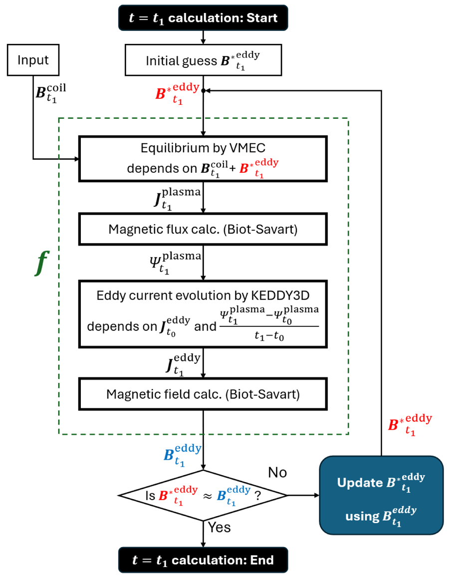
Figure 1. Flow of the evolution calculation to obtain the magnetic field produced by consistent eddy currents at $t=t_1$ . Here, $\boldsymbol {J}^{\text {plasma}}$
 and $\boldsymbol {J}^{\text {eddy}}$
 represent the plasma current and the eddy currents, $\boldsymbol {B}^{\text {eddy}}$
 denotes the magnetic field produced by $\boldsymbol {J}^{\text {eddy}}$
 , $\varPsi ^{\text {plasma}}$
 denotes the magnetic flux produced by $\boldsymbol {J}^{\text {plasma}}$
 and $\boldsymbol {B}^{\text {coil}}$
 denotes the magnetic field produced by the coil current. The subscript of each variable indicates the value at the time step. The processes enclosed by the dashed line correspond to the calculations represented by function $\boldsymbol {f}$
 in the text.
For updating ${\boldsymbol {B}^{*}}^\text {eddy}_{t_1}$ , the simplest approach is to replace the provisional magnetic field ${\boldsymbol {B}^{*}}^\text {eddy}_{t_1}$
 by the output $\boldsymbol {B}^\text {eddy}_{t_1}$
 from the previous iteration. Before introducing the proposed iteration scheme, we consider the consequence of such a simple update scheme. This corresponds to providing $\boldsymbol {B}^\text {eddy}_{t_1}$
 directly through the blue ‘Update’ box in figure 1 without any modification, allowing it to become the next ${\boldsymbol {B}^{*}}^\text {eddy}_{t_1}$
 . When using this simple update method, the calculation often diverges instead of converging, due to a nature of the VMEC's calculation. As an example, consider applying a magnetic perturbation, referred to as a ‘kick’, directed downwards to a vertically elongated plasma by providing $\boldsymbol {B}^\text {coil}_{t_1}$
 . Regardless of the magnetic field updating scheme, when ${\boldsymbol {B}^{*}}^\text {eddy}_{t_1} = \boldsymbol {B}^\text {eddy}_{t_0}$
 is given as the initial guess, the output of VMEC results in an upwardly displaced equilibrium. This outcome arises because, to restore force balance within the fixed input magnetic field distribution, which is a vertically unstable configuration, the equilibrium must shift upwards to obtain the upward electromagnetic force. Eddy currents induced by this displacement exert a downward force that pushes the plasma back. If the magnetic field is simply updated, the added downward electromagnetic force from the eddy currents yields an equilibrium with an even further upward displacement in the subsequent iteration. A specific example of such divergent behaviour is presented in § 3.2. To achieve consistent results, it is essential to apply a magnetic field update strategy that guides the calculations towards convergence.
2.2. Optimisation of adjustable parameter $\alpha$

This subsection describes how to update the magnetic field using an adjustable parameter.
The problem defined in § 2.1 for achieving convergence is organised using mathematical expressions. For simplicity, the magnetic field produced by the eddy currents at $t_1$ will be denoted as $\boldsymbol {B}$
 . Note that all variables refer to their values at $t=t_1$
 unless otherwise specified. Since the vacuum magnetic field map provided to VMEC should be given at discrete points in cylindrical coordinates, the magnetic field vector array $\boldsymbol {B}$
 has components in the $(R, \phi, Z)$
 directions and a spatial distribution for the discrete $(R, \phi, Z)$
 grid. If the number of grid points is $n$
 , it can be expressed as $\boldsymbol {B} \in \mathbb {R}^{3n}$
 . The magnetic field vector at a spatial point $i$
 is denoted by $\boldsymbol {B}_{(i)}$
 , and the magnitude of its $x$
 component ($x$
 can be $R$
 , $\phi$
 or $Z$
 ) is further denoted by $B_{(i)x}$
 .
.
The sequence of equilibrium and eddy current calculations, as illustrated in figure 1, is represented by the function $\boldsymbol {f}$ . The function $\boldsymbol {f}$
 takes $\boldsymbol {B}$
 as its input variable and outputs the magnetic field, $\boldsymbol {f}[\boldsymbol {B}]$
 , produced by the newly calculated eddy currents. Here, $\boldsymbol {f}$
 is a mapping from a magnetic field distribution vector of size $3n$
 to another magnetic field distribution vector of the same size, $\boldsymbol {f} \colon \mathbb {R}^{3n} \mapsto \mathbb {R}^{3n}$
 . Note that this mapping is nonlinear and includes MHD equilibrium and eddy current calculations. If the input magnetic field distribution $\boldsymbol {B}$
 is equal to the output magnetic field distribution $\boldsymbol {f}[\boldsymbol {B}]$
 , the whole calculation is regarded as being converged, where the self-consistent solution of the MHD equilibrium and eddy current distribution is obtained. In other words, obtaining a self-consistent solution can be interpreted as a problem of finding an input $\boldsymbol {B}$
 such that it is a ‘fixed point’ that is not changed by the mapping $\boldsymbol {f}$
 . To make the problem numerically solvable, it is transformed into an optimisation problem. We define the variation in the magnetic field distribution by $\boldsymbol {f}$
 as
as
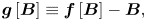
which serves as the residual vector array. The aim is to bring this $\boldsymbol {g}[\boldsymbol {B}]$ closer to the zero vector.
Since $\boldsymbol {f}$ includes equilibrium calculation and exhibits nonlinearity, it is impractical to find an exact solution in a single step. We consider an iterative approach that gradually converges to an exact solution.
Here, we define an adjustable parameter $\alpha$ and propose a simple method to optimise it. Due to the large number of dimensions of the input and output variables, it is difficult to determine the dependence of $\boldsymbol {g}[\boldsymbol {B}]$
 on $\boldsymbol {B}$
 , so the usual gradient method cannot be applied. Therefore, with the provisional magnetic field distribution as $\boldsymbol {B}^*$
 , the arbitrary magnetic field variation as $\boldsymbol {b}$
 and the adjustable parameter as $\alpha$
 , the magnetic field update shall proceed by finding a value of $\alpha$
 that makes $\boldsymbol {g}[\boldsymbol {B}^*+\alpha \boldsymbol {b}]$
 smaller. For example, if $\boldsymbol {b}$
 is a variation which makes $\boldsymbol {g}$
 smaller, then $\alpha$
 should take a positive value; conversely, if the variation makes $\boldsymbol {g}$
 greater, $\alpha$
 should take a value of zero or negative. The specific method for determining $\boldsymbol {b}$
 will be discussed in § 2.3, so we will not go into detail here.
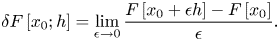
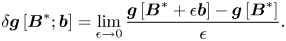
The following describes how to estimate $\boldsymbol {g}[\boldsymbol {B}^*+\alpha \boldsymbol {b}]$ based on the idea of the Gâteaux differential (Hazewinkel Reference Hazewinkel1995). Given linear topological spaces $X$
 and $Y$
 and a map $F \colon X\mapsto Y$
 , the Gâteaux differential in the direction $h \in X$
 at $x_0 \in X$
 is expressed as follows:
The parameter $\delta F[x_0; h]$ on this left-hand side is called the Gâteaux variation, and the Gâteaux variation has homogeneity of degree 1 with respect to $h$
 , namely
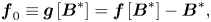
holds for any scalar $\alpha$ . If we apply the Gâteaux differential to the current problem, we obtain the following expression:
Here, the Gâteaux variation $\delta \boldsymbol {g}$ is just a vector of the $\mathbb {R}^{3n}$
 directional derivatives of each real-valued components of $\boldsymbol {g}$
 along the direction of the specific vector $\boldsymbol {b}$
 . Now consider approximating the limit operation by a finite-width difference operation, as is done in general numerical differentiation. Using an appropriate positive constant $\epsilon _{c}$
 , we denote the approximated Gâteaux variation as follows:
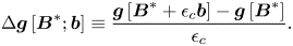
This approximate Gâteaux variation (2.5) will reproduce the original Gâteaux variation (2.4) if $\epsilon _{c}$ is small enough. Assuming that $\epsilon _{c}$
 is small enough to make $\delta \boldsymbol {g} \approx \Delta \boldsymbol {g}$
 hold for $\boldsymbol {b}$
 and $\alpha \boldsymbol {b}$
 , the following approximation holds due to the homogeneity shown in (2.3):

The implication of this expression is that the variation of $\boldsymbol {g}$ is approximately homogeneous for small changes in input. Let us now consider the case where $\epsilon _c=1$
 in order to make (2.6) an expression for $\boldsymbol {g}[\boldsymbol {B}^* + \alpha \boldsymbol {b}]$

This condition can be also interpreted as that the exact derivative is replaced by a finite differences approximation. This formula becomes less accurate the larger $\boldsymbol {b}$ is, but as a rough approximation it can be considered to hold for any $\boldsymbol {b}$
 . Even if $\boldsymbol {b}$
 is so large that the approximation is completely invalid, (2.7) can be made valid by redefining $\boldsymbol {b}$
 as a reduction to a suitable scale. Gathering terms in (2.7) with respect to $\alpha$
 , we obtain

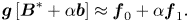
Based on (2.7), the value of $\alpha$ will be determined such that $\boldsymbol {g}[\boldsymbol {B}^* + \alpha \boldsymbol {b}]$
 becomes smaller. Here, we propose two policies. One policy is to aim for the average value of each component going to zero, and the other is to aim for the mean of the sum of squares of the components being a local minimum.
First, the policy to reduce the average value of each component to zero is considered. If expression (2.10) is separated in components, it can be rewritten as
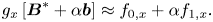
This expression is simply a reformulation of expression (2.10), without introducing any new assumptions. From (2.11), we can find $\alpha$ such that the average value of each component of the residual becomes zero, but such an $\alpha$
 will be different for each component. Since it is necessary to reduce all components to bring $\boldsymbol {g}$
 close to zero, it is desirable to optimise each component simultaneously. Therefore, we allow $\alpha$
 to take different values for each component and consider treating $\alpha$
 as a vector
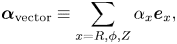
where $\boldsymbol {e}_x$ is the unit vector for the $x$
 -direction. When using $\boldsymbol {\alpha }_\text {vector}$
 , the initially assumed updated magnetic field $\boldsymbol {B}^* + \alpha \boldsymbol {b}$
 is modified to $\boldsymbol {B}^* + \boldsymbol {\alpha }_\text {vector}\odot \boldsymbol {b}$
 , where the symbol $\odot$
 denotes component-by-component multiplication. One might question the modification of the starting formula in the discussion, but we have merely relaxed the implicit constraint that $\alpha$
 is a scalar. To adapt $\boldsymbol {\alpha }_\text {vector}$
 , the expression (2.7) can be modified to a component-wise approximation formula

where we remind the reader that $x$ stands for $(R, \phi, Z)$
 . Using the symbol $odot$
 , it reads
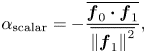
To make the spatially averaged residuals for each $x$ component vanishing, $\alpha _x$
 is determined by

Here, the overline denotes averaging over the spatial distribution. If $S_\text {in}$ denotes the region for averaging and $n_\text {in}$
 denotes the number of spatial points in $S_\text {in}$
 , then $\bar {\boldsymbol {B}}\equiv ({1}/{n_\text {in}})\sum _{i\in S_\text {in}}{\boldsymbol {B}_{(i)}}$
 . Since applying independent operations to each component may result in a magnetic field distribution that is not divergence free, it is necessary to address this issue in the implementation to obtain an appropriate magnetic field distribution. This point will be discussed in § 2.3.
In general, independence of each component of $\boldsymbol {g}$ is not exactly established, but a rough component-by-component correspondence is thought to exist. Since changes in the input magnetic field move the plasma and the eddy currents are induced to suppress it, it can be inferred that there is a correspondence between the changes in input and output of $\boldsymbol {f}$
 in each spatial direction. Furthermore, because the cylindrical coordinate system is orthogonal, the direction of a spatial vector can be represented by a combination of independent components. From these considerations, it can be assumed that the solution by (2.15) brings $\boldsymbol {g}$
 closer to the zero vector, even though strict independence is not established.
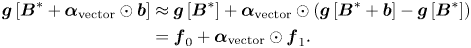
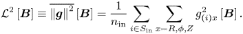
Next, the policy of minimising the sum of squares of the components is considered. The spatial average of the sum of squares of $\boldsymbol {g}$ is denoted $\mathcal {L}^2$
 as follows:
Then, $\mathcal {L}^2[\boldsymbol {B}^* + \alpha \boldsymbol {b}]$ can be estimated using (2.10) as

and the derivative for $\alpha$ is
is
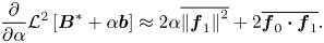
From (2.18), $\mathcal {L}^2$ takes a local minimum value at
which is the solution for the second policy. Although this solution is equivalent to what has been described briefly in a reference work (Cianciosa et al. Reference Cianciosa, Isernia, Rubinacci, Terranova and Villone2021), here, we have given its derivation more consistently. There could be a variety of theoretically possible optimisation policies other than the two proposed here, but we did not find any very promising ones as far as we tried.
The described method can be interpreted as a single-variable optimisation approach for the parameter $\alpha$ , representing a step size in a specific search direction, using Newton's method. The policy of treating $\alpha$
 as a vector constitutes a root-finding problem for the spatially averaged values of each component, whereas treating $\alpha$
 as a scalar represents a least-squares problem. This approach may also resemble the secant method, as it employs a secant defined by two points, $\boldsymbol {B}^*(\alpha =0)$
 and $\boldsymbol {B}^*+\boldsymbol {b}(\alpha =1)$
 ; however, since the correspondence between the value of $\alpha$
 and the actual magnetic field distribution varies with each iteration, the proposed method differs from the conventional secant method, which uses the result from the previous iteration to give one of the points defining the secant taken from the result of the previous iteration.
2.3. Implementation
This subsection explains the specific implementation of the method described in § 2.2 into numerical calculations.
In this study, the variation $\boldsymbol {b}$ in the input magnetic field is given by the residual vector for the provisional magnetic field

as the search direction in which some variation in $\boldsymbol {g}$ is expected, whether positive or negative. Since $\boldsymbol {g}[\boldsymbol {B}^*]$
 is required for determining $\alpha$
 in any case, it can be used for both purposes to reduce the number of times $\boldsymbol {f}$
 needs to be evaluated. The property of $\boldsymbol {g}[\boldsymbol {B}^*]$
 becoming smaller as the convergence progresses is convenient because it automatically scales $\boldsymbol {b}$
 appropriately in iterative calculations, and leads to a better approximation accuracy of the approximation (2.7). This approach to determining $\boldsymbol {b}$
 does not guarantee the most effective reduction of $\boldsymbol {g}$
 ; however, it is practical as it does not require gradient calculations and allows for the straightforward use of VMEC.
Next, the update formula for $\boldsymbol {B}^*$ is considered. Although $\alpha$
 was determined in § 2.2 to make $\boldsymbol {g}[\boldsymbol {B}^*+\alpha \boldsymbol {b}]$
 smaller, it remains open to consideration whether $\boldsymbol {g}[\boldsymbol {B}^*+\alpha \boldsymbol {b}]$
 should be used as it is as an update formula for $\boldsymbol {B}^*$
 . Since the final solution is the output of $\boldsymbol {f}$
 , $\boldsymbol {B}^*$
 should be a physical solution which is a possible result of the equilibrium and eddy current calculations. It is not guaranteed that a solution equal to $\boldsymbol {B}^*+\alpha \boldsymbol {b}$
 will be given by the results of the series of calculations, even if $\boldsymbol {B}^*$
 is a physical solution, because $\boldsymbol {B}^*+\alpha \boldsymbol {b}$
 is numerically deformed from $\boldsymbol {B}^*$
 . For example, $\boldsymbol {B}^*+\boldsymbol {\alpha }_\text {vector}\odot \boldsymbol {b}$
 is not a physically appropriate solution because it does not keep solenoidality due to the deformation by $\boldsymbol {\alpha }_\text {vector}$
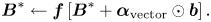
 . Therefore, especially when $\alpha$
 is treated as a vector, the output of $\boldsymbol {f}$
 with $\boldsymbol {B}^*+\boldsymbol {\alpha }_\text {vector}\odot \boldsymbol {b}$
 as input is adopted as the provisional magnetic field $\boldsymbol {B}^*$
 for the next iteration, namely
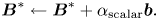
On the other hand, the increase in the number of evaluations of $\boldsymbol {f}$ is not desirable for computational efficiency. Considering that $\boldsymbol {B}^* + \boldsymbol {b} = \boldsymbol {f}[\boldsymbol {B}^*]$
 is a physical solution when (2.20) is adopted, $\boldsymbol {B}^*+\alpha _\text {scalar}\boldsymbol {b}$
 is a mixture of two physical solutions, a distribution that is possible as a result of eddy current calculation (although the existence of equilibrium calculation results that induce such eddy currents is still not guaranteed). Therefore, when $\alpha$
 is a scalar, $\boldsymbol {B}^*+\alpha _\text {scalar}\boldsymbol {b}$
 has a small deviation from physical solutions, and the following update formula can be used:
Comparing formulae (2.21) and (2.22), it should be noted that treating $\alpha$ as a vector requires one extra evaluation of $\boldsymbol {f}$
 . Figure 2 shows a flowchart based on the implementation methods described so far, which represents the contents of one iteration of the convergence calculation.
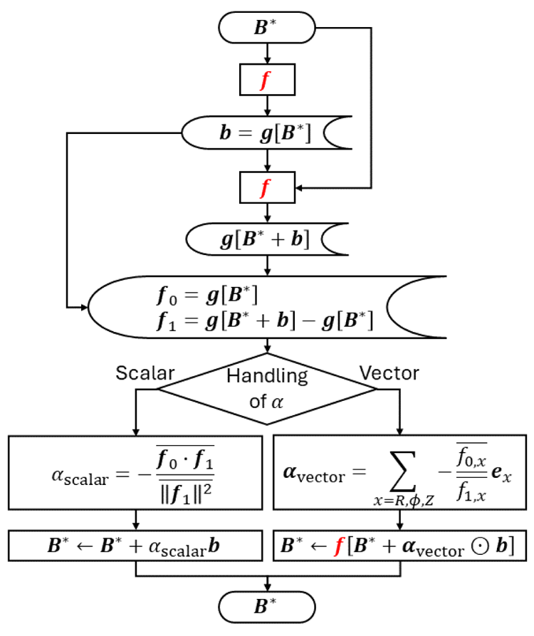
Figure 2. Flowchart showing one iteration of the convergence calculation to update the provisional vacuum magnetic field distribution $\boldsymbol {B}^*$ .
.
One point to note in the implementation is the numerical divergence in expression (2.15). On the right-hand side of (2.15), there are cases where the denominator is almost zero but the numerator is a finite value, making $\alpha _x$ extremely large. To avoid such a problem, it is recommended to provide an appropriate upper limit for the value of $\alpha _x$
 (e.g. a fixed value or a value set with reference to the value of $\alpha _\text {scalar}$
 ).
).
3. Validation calculations
In this section, the method described in § 2 is verified by performing evolution calculations of equilibrium. After applying total toroidal current decay to the initial equilibrium, evolution calculations are performed for one time step to check the validity of the results. The evolution calculations are carried out by convergence calculation with a specified number of iterations, and the process of convergence is also investigated.
The parameters for the initial equilibrium and the calculation settings are shown in table 1, and the parameters for the conductive wall are shown in table 2. The radial profiles of pressure $p$ and the normalised radial derivative of the flux-averaged toroidal current density $I^\prime$
 are shown in figure 3. In this study, the radial profile of normalised toroidal current density is kept unchanged, and only the total toroidal current magnitude is varied.
Table 1. Parameters of the initial equilibrium plasma.
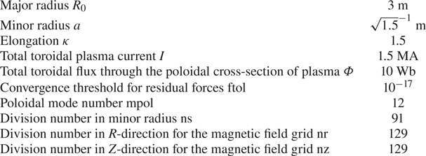
Table 2. Parameters of the conductive wall.
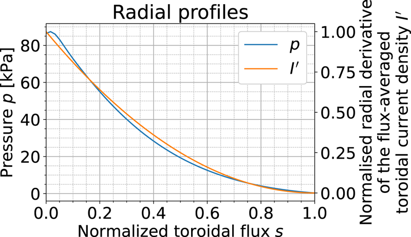
Figure 3. Radial profile of pressure $p$ and the normalised radial derivative of the flux-averaged toroidal current density $I^\prime = 1 - 2s + s^2$
 , where $s$
 is the normalised toroidal magnetic flux.
The initial plasma boundary, conductive wall and poloidal coil configuration are shown in figure 4. The plasma shape was determined by adjusting the external coil current so that the result of the free boundary equilibrium calculation follows the representation

in the poloidal angle $\theta$ as closely as possible. The calculations in this section were performed in axisymmetric settings. Poloidal eddy currents are not considered in KEDDY3D in axisymmetric calculations.
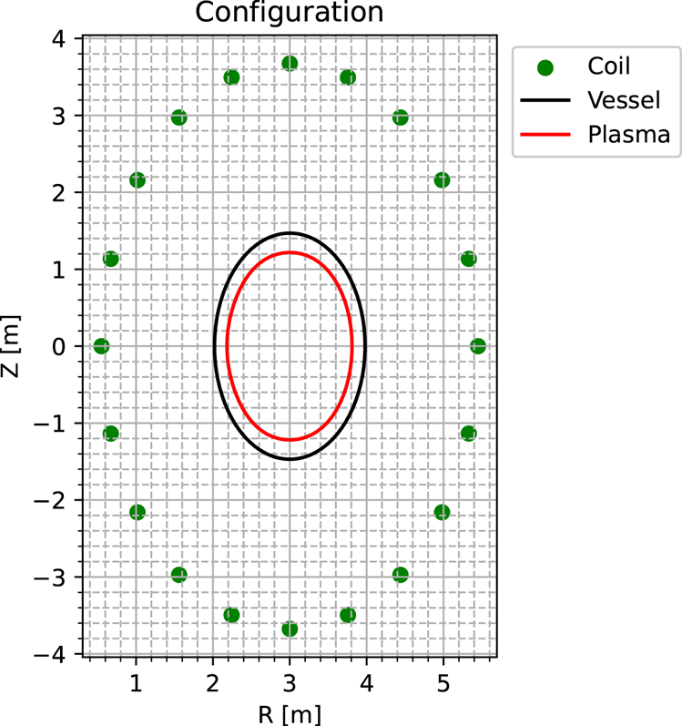
Figure 4. Configuration of the initial equilibrium plasma, conductive wall and coils.
Cases that only include displacements in the horizontal direction, the physically stable direction, are treated in § 3.1, and cases that also include displacements in the vertical direction, the unstable direction, are treated in § 3.2. The results for the case of simple update without using the proposed method are observed first, then the calculation results using the proposed method are verified. Unless otherwise mentioned, the time step width is 1 ms and the current decrease given as a fluctuation is 1 % of the total toroidal current. The iterative calculation is not terminated by the convergence, but is iterated a specified number of times.
3.1. Horizontal displacement
This subsection deals with the case where only horizontal displacements are induced by the reduction of the total toroidal plasma current.
3.1.1. Results for simple update
We first illustrate the results obtained when using a simple update method, where the output magnetic field from the previous iteration is directly used as the input for the next iteration, expressed by the substitution equation as $\boldsymbol {B}^* \leftarrow \boldsymbol {f}[\boldsymbol {B}^*]$ , without employing the method described in § 2.
Figure 5 shows the results of iterative calculations for 10 iterations. In figure 5(b), which shows the change in the horizontal position of the magnetic axis, the results using the proposed method in § 2 is also plotted for comparison (these results will be discussed in § 3.1.2). One iteration means a series of calculations to update the vacuum field distribution. The label ‘Simple update’ in figure 5(b) represents the results obtained using the simple magnetic field update method, corresponding to the outcome shown in figure 5(a). The labels ‘$\boldsymbol {\alpha }_\text {vector}$ ’ and ‘$\alpha _\text {scalar}$
 ’ refer to the series of calculations shown in figure 2.
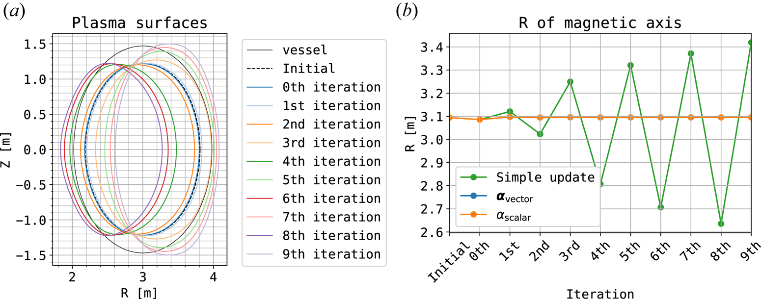
Figure 5. Changes in the plasma shape and the position of magnetic axis during a simple iterative calculation with alternating updates of equilibrium and eddy currents, following a 1 % decrease in total toroidal current. (a) Shows the plasma surfaces. The grey line represents the conductor simulating the VV with flowing eddy currents. The dashed line shows the initial equilibrium plasma shape before the current decreases, while the solid coloured lines show the equilibrium plasma shapes after the current decreases. (b) Shows the horizontal positions of the magnetic axis during the iterations. The green line is the result of simple updates, and the blue and orange lines are examples of the result using the proposed method.
From figure 5(a), it can be seen that the plasma is significantly displaced and deformed by the iterative calculations with simple update, and the calculation results do not converge. ‘Simple update’ in figure 5(b) shows that the amplitude is increasing, with the direction of displacement reversing in each iteration. Focusing on the 0th and 1st iterations in 5(b), at the 0th iteration, all results show the inward displacement due to the current decrease, but at the 1st iteration, the magnetic axis of ‘Simple update’ is located obviously outside the initial position, while ‘$\boldsymbol {\alpha }_\text {vector}$ ’ and ‘$\alpha _\text {scalar}$
 ’ quickly settle near the final convergence position. Based on the equilibrium displaced outward from the initial position (the position at the previous time step), the eddy currents are induced to push the plasma back inward. As a result, in the 2nd iteration, adopting the magnetic field produced by these eddy currents, the plasma becomes even more excessively displaced inward compared with the 0th iteration. In other words, during the convergent iteration of evolution involving horizontal displacement, although the initial displacement occurred in a physically reasonable direction, the excessive magnitude of the displacement led to oscillatory divergence in the behaviour.
The results in figure 5 demonstrate that simple updates cannot correctly calculate the evolution of the equilibrium considering eddy currents, although the simulation set-up is very simple. Since the same behaviour was observed even when the time step or the amplitude of current decay was changed, this behaviour is considered to be a qualitative instability caused by the computational scheme rather than numerical instabilities (e.g. instability due to the time step width). Given that this behaviour subsides when the resistivity of the VV is increased or the distance between the plasma and VV is enlarged, such behaviour should be specific to situations where a sufficiently conductive wall is present.
3.1.2. Results for the proposed method
The results of using the proposed method in the current reduction simulation are presented here and the differences due to the treatment of $\alpha$ are discussed.
Figure 6 visualises the histories of the residual metric $\mathcal {L}^2[\boldsymbol {B}^*]$ defined in (2.16) during the convergence calculation. In both ‘$\boldsymbol {\alpha }_\text {vector}$
 ’ and ‘$\alpha _\text {scalar}$
 ’, $\mathcal {L}^2$
 gets smaller with iterations, reaching a value of order $1\times 10^{-20}$
 , which appears to be due to numerical errors. Although there appears to be no significant difference in the global convergence speed, the actual computational cost is smaller for ‘$\alpha _\text {scalar}$
 ’ because one extra evaluation of $\boldsymbol {f}$
 is required in ‘$\boldsymbol {\alpha }_\text {vector}$
 ’, as shown in figure 2.
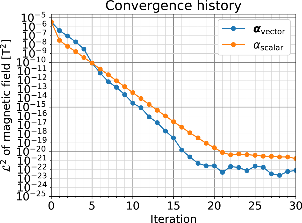
Figure 6. History of decrease in $\mathcal {L}^2$ of the magnetic field during convergence calculation for temporal development with the plasma toroidal current decrease. The label $\boldsymbol {\alpha }_\text {vector}$
 represents that $\alpha$
 is treated as a vector and $\alpha _\text {scalar}$
 represents that the parameter $\alpha$
 is treated as a scalar.
3.2. Combination of horizontal and vertical displacements
This subsection examines the calculations in the presence of vertical displacement in addition to the horizontal one.
By shifting the VV by ${+0.1}\ {\rm m}$ in the $Z$
 -direction, the relative initial position of the plasma is shifted downwards. This operation can be interpreted as placing the initial equilibrium plasma below the neutral equilibrium location for the vertical displacement events (Nakamura et al. Reference Nakamura, Yoshino, Neyatani, Tsunematsu, Azumi, Pomphrey and Jardin1996). The physical mechanism is that the eddy currents induced by the reduced plasma current are in the same direction as the plasma current, so the attraction between the same direction currents should cause the plasma to displace downwards (nearer side to VV), while also inducing eddy currents to suppress it. Naturally, there is also the inward shift of the plasma due to current damping, as in § 3.1, so the situation is complicated by a combination of horizontal and vertical displacements.
3.2.1. Results for simple update
As in § 3.1.1, the result of the case without using the proposed method is checked first.
In this case, blend update is applied instead of the simple update to suppress the horizontal displacement. Otherwise, the calculation would collapse due to increasing horizontal displacements as in figure 5 before the vertical displacements become significant. In blend update, the current provisional magnetic field is blended to the new magnetic field when updating the magnetic field as $\boldsymbol {B}^* \leftarrow (\boldsymbol {B}^* + \boldsymbol {f}[\boldsymbol {B}^*])/2$ . In order to ensure that a visible change appears, in this calculation the total toroidal plasma current decrease was set to 5 % instead of 1 %.
Figure 7 shows the history of the plasma shape and the vertical position of the magnetic axis in convergence calculations. From figures 7(a) and 7(b), it can be seen that the vertical displacement increases monotonically for the blend update without using the proposed method.
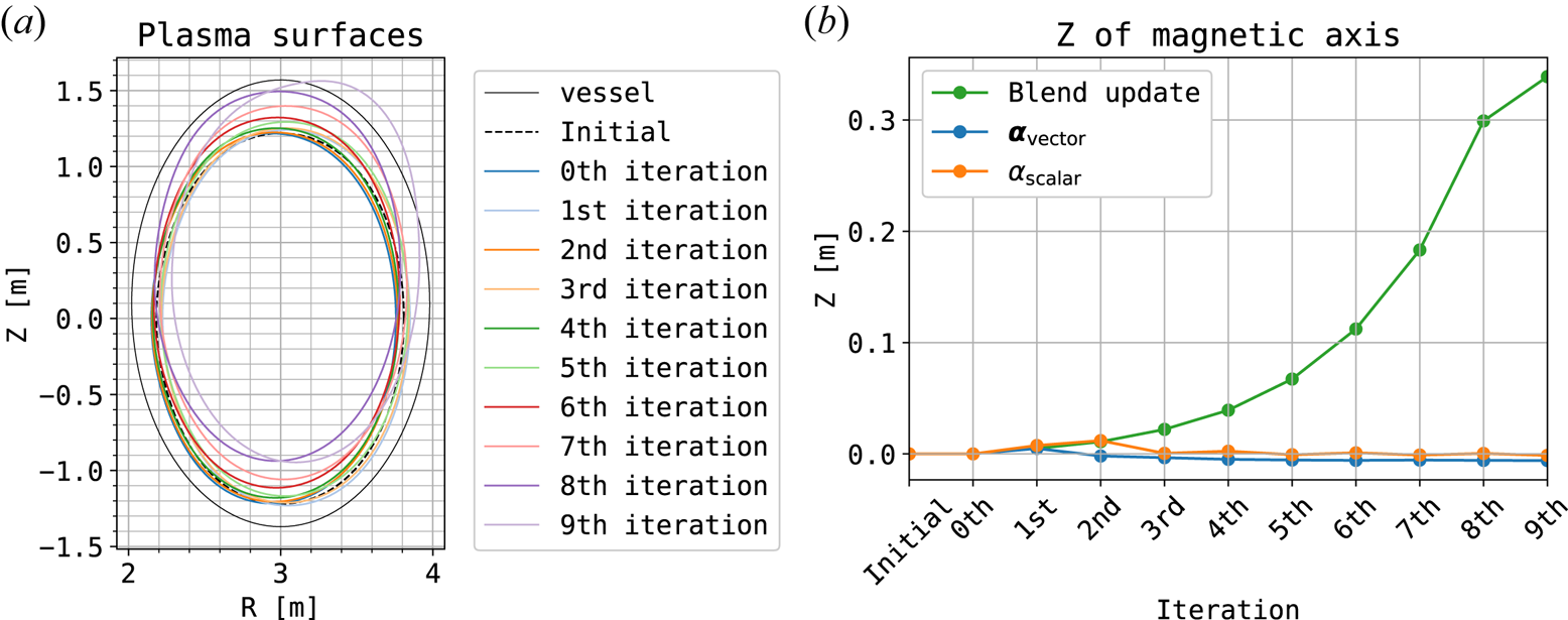
Figure 7. Changes in the plasma shape and the position of the magnetic axis during a simple iterative calculation with alternating updates of equilibrium and eddy currents, adopting blend update, following a 5 % decrease in total toroidal current. The VV is shifted ${+0.1}\ {\rm m}$ in the $Z$
 -direction from the position shown in figure 4. (a) Shows the plasma surfaces. (b) Shows the vertical positions of the magnetic axis during the iterations.
Focusing on the direction of displacement, the displacement is occurring in the upward direction, contrary to the physical mechanism. This behaviour is thought to be exactly due to the mechanism described in § 2.1. It is shown that, by repeating equilibrium calculations with a fixed input magnetic field distribution and eddy current calculations based on the equilibrium plasma, displacements in the direction opposite to the electromagnetic force are amplified.
What the results in § 3.1.1 and this section show is that the relationship between plasma displacement and eddy currents can vary with direction, in the VMEC calculation. In equilibrium calculations, the plasma shape is determined such that the residual forces acting on the plasma are minimised. However, in calculations where the input magnetic field is fixed, the displacement direction that reduces the residual force corresponds to the same direction as the residual force in the stable direction and the opposite direction in the unstable direction. Physically, eddy currents are induced to exert forces that suppress the displacement from the previous time step, and the magnetic field produced by the eddy currents works to suppress displacement in the stable direction, as shown in figure 5, and amplify it in the unstable direction in the next equilibrium calculation, as shown in figure 7.
3.2.2. Results for the proposed method
The results of the proposed method are discussed in this section. To keep consistency with the results in figure 7, the current decrease is set to 5 % as in § 3.2.1.
Figure 8 visualises the histories of $\mathcal {L}^2[\boldsymbol {B}^*]$ during the convergence calculation. Whereas $\mathcal {L}^2$
 decreases with each iteration and reaches the order of numerical error as in figure 6 for ‘$\boldsymbol {\alpha }_\text {vector}$
 ’, the decrease in $\mathcal {L}^2$
 almost stops progressing at of the order of $1\times 10^{-8}$
 for ‘$\alpha _\text {scalar}$
 ’. As can be seen in figure 7, the vertical position of the magnetic axis in ‘$\alpha _\text {scalar}$
 ’ oscillated around zero, and the vertical displacement did not seem to converge to the correct result. This behaviour can be explained by the different characteristics depending on the direction of displacement, also mentioned in § 3.2.1. In the horizontal direction, the eddy currents act in the direction of suppressing displacement. The residual vector, which is the change from input to output of $\boldsymbol {f}$
 , is therefore a magnetic field in the direction of suppressing the displacement of the plasma, and the sign of the appropriate $\alpha _\text {scalar}$
 in formula (2.22) is usually positive. In the vertical direction, on the other hand, the eddy currents act in the direction of amplifying the displacement, so the appropriate $\alpha _\text {scalar}$
 is negative. In ‘$\alpha _\text {scalar}$
 ’, the magnetic field is updated using a single $\alpha _\text {scalar}$
 regardless of the direction, so an update that simultaneously suppresses displacements in both directions is basically impossible. In particular, ‘$\alpha _\text {scalar}$
 ’ is based on local minimisation of $\mathcal {L}^2$
 , so it tends to stay in the local solution, and no matter how far the iterations are increased, it is unlikely to move towards the correct solution.
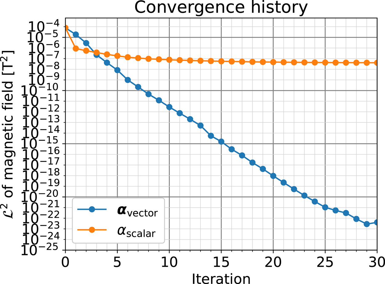
Figure 8. History of decrease in $\mathcal {L}^2$ of the magnetic field during convergence calculation for temporal development with the toroidal plasma current decreasing.
From this result, it can be concluded that the policy of treating $\alpha$ as a scalar may not be effective and that it is preferable to adopt the policy of treating $\alpha$
 as a vector. inputsections/application
4. Application to non-axisymmetric calculation
In this section, a non-axisymmetric simulation of plasma evolution is carried out using the proposed method. The calculation method described in § 2 does not contain an axisymmetric assumption and therefore can be applied directly to non-axisymmetric calculations. It will be verified whether the proposed method works well in a situation with a non-axisymmetric eddy current distribution, especially with large poloidal eddy currents.
Based on the set-up of the current decay calculation in § 3.1, a simulation is performed when a non-axisymmetric electrical resistivity distribution, which will be described later, is given to the VV. The calculation settings for the non-axisymmetric calculation are shown in table 3. The initial plasma shape is set to be axisymmetric, as in § 3, but during the simulation the magnetic surface geometry is allowed to have non-axisymmetry as follows:


where $\theta$ and $\zeta$
 are poloidal and toroidal angles. The evolution calculation is carried out for 25 time steps, with a time step width of 1 ms per step and the current decay rate of ${15}\ {\rm kA}\ {\rm ms}^{-1}$
 , as in § 3. For convergence calculations, the policy of treating $\alpha$
 as a vector was adopted.
Table 3. Parameters for non-axisymmetric calculation.
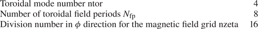
To illustrate the given electrical resistivity distribution, the density distribution and streamlines of eddy currents at the final step of the simulation induced by plasma current decay are visualised by ParaView in figure 9. A bellows-like resistivity distribution is given to limit the toroidal eddy current so that poloidal eddy currents are generated. The plasma and VV is set to have a periodicity of eight cycles in the toroidal direction. A toroidal width corresponding to one eighth of one cycle in VV is set as the insulating section, with the resistivity in the toroidal direction $1\times 10^{6}$ times that of the rest. The insulating sections correspond to the region where the blue line structure appears in the poloidal direction in the figure. The toroidal plasma current decay induces toroidal voltage on VV, but the presence of insulating sections makes it difficult for toroidal eddy currents to flow, so poloidal currents are generated in conducting sections. As a result, a saddle-shaped structure of the streamline appears in the conductive sections, which is typical for VV with bellows. It should be noted that the insulating sections not only change the eddy current structure, but also simply increase the effective electrical resistance in the toroidal direction, so that the stabilising effect on plasma displacement due to the eddy currents is weaker compared with the axisymmetric calculation.
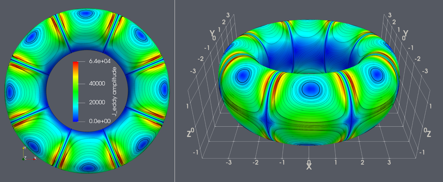
Figure 9. Eddy current density distribution at the final step of the simulation of plasma current decay. Colours represent the density of eddy current, and black lines represent streamlines of current flow. The saddle-shaped structures due to the set-up of the insulating sections appear on the conductive sections. The direction of current flow in the saddle-shaped structure is counterclockwise on the figure at the left-hand side.
From here on, the result of the simulation is discussed. Convergence calculation at each time step showed that the residuals decreased smoothly at each iteration, with $\mathcal {L}^2$ converging to the order of $1\times 10^{-22}$
 or less at each time step. This confirms that the proposed method works well for non-axisymmetric calculations.
To confirm the non-axisymmetric deformation of the plasma, figure 10 shows the plasma surface in the final results with exaggeration of the non-axisymmetric component by a factor of 200. Note that the figure shows numerical exaggerations to make the relationship between plasma deformation and eddy currents clear to see, but the actual deformation is so small that it is not visible on the scale of the entire device. The $Z$ -directional components of the plasma current and eddy currents plotted in colour in figure 10 show that the plasma is deformed so that the plasma is close to the wall in areas where the signs of both currents coincide and vice versa. This is thought to be a natural consequence of the attraction and repulsion forces between currents.
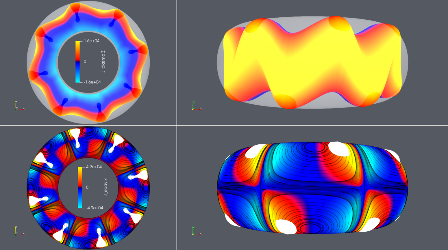
Figure 10. The plasma surface geometry with the $n\neq 0$ mode exaggerated 200 times. The $Z$
 -directional components of the plasma current and eddy currents are projected as colours. The top row is coloured for plasma current, and the bottom row is coloured for eddy currents. The left column shows the viewpoint from the $+Z$
 side and the right column from the $-Y$
 side. The streamlines are overlaid on the eddy currents.
To assess the magnitude of the actual (not exaggerated) plasma deformation, heat maps of the Fourier coefficients in expressions (4.1) and (4.2) for the outermost magnetic surface of the plasma in the VMEC output at the final time step are shown in figure 11. As per expression (3.1a,b), the shape of the initial equilibrium is represented by $R_{0,0}^\text{c}=R_0$ , $R_{1,0}^\text{c}=a$
 and $Z_{1,0}^\text{s}=\kappa a$
 . We shall only focus on the $n\neq 0$
 component. The largest amplitude of $n\neq 0$
 component in figure 11 is $Z_{0,1}^\text{s}={1.47}\ {\rm mm}$
 , which leads to a deformation of the whole plasma surface that ripples up and down. Taking into account the other $m=0, n>1$
 components as well, the waveform of $Z$
 should be a sine curve which has a shifted peaks closer to the insulating sections, as shown in the top right-hand view in figure 9. Note that the toroidal angle $\zeta$
 corresponds to $\arctan {Y/X}$
 in the coordinates of 3-D diagrams, namely the centres of the conductive section located at $\zeta =({{\rm \pi} }/{4})i$
 ($i$
($i$ is an arbitrary integer). The $m>1$
 components form a checkerboard-like waveform in the $\theta\zeta\theta\zeta$
 plane because the $\pm n$
 component pairs have opposite signs and comparable amplitudes, roughly corresponding to the distribution of the $Z$
 -directional component of the eddy currents in figure 9. The maximum amplitude of the $m>1$
 component is approximately 0.5 mm, indicating that the deformation is approximately 2 mm at most, even when considering the area with the largest variation together with the $m=0$
 component (corresponding to the area where the plasma protrudes from the VV in figure 9).
Figure 11. Fourier coefficients of the plasma shape. The colour ranges are bounded by the maximum absolute value of the $n\neq 0$ components. The numbers inside the boxes indicate the Fourier coefficients of each mode, the same as the colour bar (to display values outside the range of the colour bar). The remaining components $R_{mn}^\text{s}$
 and $Z_{mn}^\text{c}$
 are omitted because their amplitudes were almost zero for all modes.
Finally, the magnetic field ripple, which is important in plasma behaviour, is evaluated. The ripple rate of the magnetic field intensity is shown in figure 12. The ripple rate is defined here as the percentage of deviation from the mean value on the toroidal loop at a constant radial coordinate $s$ and constant poloidal angle $\theta$
 in the left-handed VMEC coordinate system $(s, \theta, \zeta )$
 . From figure 12, it can be seen that the ripple rate is mainly high in areas of large deformation, with an amplitude of around 0.5 %.
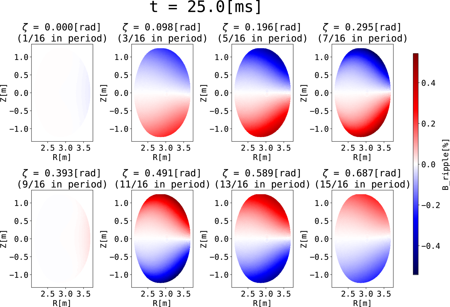
Figure 12. Mapping of the ripple rates of the magnetic field on the poloidal cross-sections of plasma. Toroidal angles are shown every other one with respect to the grid.
As a conclusion of the applied calculation to the non-axisymmetric case, the calculations with the proposed method converged stably over a long time step and the results were physically explainable.
5. Conclusion
A convergence method for the time-dependent calculation of MHD equilibrium and eddy currents is proposed towards the development of a non-axisymmetric disruption simulation code. The method combines independent codes for MHD equilibrium and eddy current calculations to achieve self-consistent coordination through external processing without modifying the contents of each.
The main contributions of this paper are twofold: (i) the formulation of the convergence calculations for equilibrium and eddy currents as a optimisation problem, and (ii) the proposal of a policy that can deal with different characteristics of displacement depending on the direction, based on a component-by-component representation of the approximate expression for the residual vectors.
The proposed method has been applied to several test cases and has been found to converge to reasonable results. The method is convenient since it does not require modifications to the content of the modular codes, making it easy to apply the method to codes other than those used in this study. However, this method requires multiple sets of calculations for one step of temporal evolution, so it could be not so good in terms of saving computational costs. It may be less computationally efficient than codes designed specifically for evolution calculation of an equilibrium with eddy currents, and we should benchmark our code against such codes in the future work.
As the proposed method successfully calculated the temporal development of equilibrium in the case of VV with non-axisymmetry, it is expected that the method can be applied to calculations considering passive coils with 3-D structures. An example of research requiring such calculations is the suppression of disruption-generated runaway electrons by passive coils (Smith, Boozer & Helander Reference Smith, Boozer and Helander2013) (Tinguely Reference Tinguely2021). The magnetic field distribution obtained by the proposed method by self-consistently solving for changes in the MHD equilibrium and the eddy currents in the passive coil can be used to simulate the trajectory of runaway electrons.
In § 3, the simulation was performed for a single time step only, but it has been confirmed that, by repeating such calculations, evolution involving vertical displacement can be handled. The validation of the physical plausibility of the calculated result, as well as the method for consistently solving variables other than the vacuum magnetic field, remain tasks for future work.
Acknowledgements
Editor Nuno Loureiro thanks the referees for their advice in evaluating this article.
Funding
This work was supported by JSPS KAKENHI Grant Number JP24KJ1412, and the establishment of university fellowships towards the creation of science technology innovation by JST Grant Number JPMJFS2123.
Declaration of interests
The authors report no conflict of interest.


 Open access