

1 Introduction
Laser-driven charged particle acceleration is an attractive alternative to standard accelerators, promising to provide a much greater acceleration rate via a much more compact facility. In the laser wake-field accelerator (LWFA) concept introduced in Tajima & Dawson (Reference Tajima and Dawson1979), a long-lived strong wake field, induced by a short intense laser pulse in its wake in a low-density collisionless plasma, accelerates duly injected electrons.
Within the framework of the laser wake-field accelerator paradigm (Tajima & Dawson Reference Tajima and Dawson1979; Esarey, Schroeder & Leemans Reference Esarey, Schroeder and Leemans2009; Hooker Reference Hooker2013) a regular and strong electric field having the form of a wave propagating with a phase velocity close to speed of light in a vacuum is excited in underdense plasmas by short pulse relativistically intense laser radiation. The electrons injected into the wake-field acceleration phase with an initial energy corresponding to the velocity equal to the wake wave phase velocity are then accelerated up to significantly higher energy. The achievable electron energy is determined by several processes among which the first is the electron slippage with respect to the accelerating phase of the wake wave and the second is the laser energy depletion. The dephasing and depletion lengths being inversely proportional to the plasma density are of the same order.
Today’s highest electron energy achieved in experiments on the single laser pulse interaction with an underdense plasma target is in the multi-GeV range being of 3 GeV in the case reported by Kim et al. (Reference Kim, Pae, Cha, Kim, Yu, Sung, Lee, Jeong and Lee2013) and above 4 GeV in the experiment (Leemans et al. Reference Leemans, Gonsalves, Mao, Nakamura, Benedetti, Schroeder, Tóth, Daniels, Mittelberger and Bulanov2014), where petawatt class lasers and targets of the size of the order of ten centimetres have been used.
The multistage LWFA system based on using succeeding accelerating stages wherein the wake waves are driven by multiple laser pulses may enable electron acceleration over distances significantly longer than the dephasing and depletion lengths (Cheshkov et al. Reference Cheshkov, Tajima, Horton and Yokoya2000; Chiu, Cheshkov & Tajima Reference Chiu, Cheshkov and Tajima2000; Leemans & Esarey Reference Leemans and Esarey2009; Schroeder et al. Reference Schroeder, Esarey, Geddes, Benedetti and Leemans2010; Nakajima et al. Reference Nakajima, Deng, Zhang, Shen, Liu, Li, Xu, Ostermayr, Petrovics and Klier2011; Mehrling et al. Reference Mehrling, Grebenyuk, Tsung, Floettmann and Osterhoff2012). The use of multi-stage LWFA accelerators also has the potential for improving the quality of the beams of the accelerated electrons (Pollock et al. Reference Pollock, Clayton, Ralph, Albert, Davidson, Divol, Filip, Glenzer, Herpoldt and Lu2011; Nakahara et al. Reference Nakahara, Mizuta, Kajino, Makito, Kodama, Hosokai, Masuda, Nakanii, Zhidkov and Kando2013; Zhang et al. Reference Zhang, Li, Liu, Wang, Yu, Tian, Nakajima, Deng, Qi and Wang2016).
The theoretical work is mainly devoted to discussing the multi-stage accelerator configurations comprised of stages of equal length and density (however, see recently published paper Zhang et al. (Reference Zhang, Liu, Wang, Li, Yu, Tian, Qi, Wang, Qin and Fang2015) where a three uneven stage accelerator has been theoretically considered). Experimentally realized multi-stage accelerators (at the moment they are two stage systems (Pollock et al. Reference Pollock, Clayton, Ralph, Albert, Davidson, Divol, Filip, Glenzer, Herpoldt and Lu2011; Kim et al. Reference Kim, Pae, Cha, Kim, Yu, Sung, Lee, Jeong and Lee2013; Steinke et al. Reference Steinke, van Tilborg, Benedetti, Geddes, Schroeder, Daniels, Swanson, Gonsalves, Nakamura and Matlis2016)) consist of plasma slabs with different density (Pollock et al. Reference Pollock, Clayton, Ralph, Albert, Davidson, Divol, Filip, Glenzer, Herpoldt and Lu2011; Kim et al. Reference Kim, Pae, Cha, Kim, Yu, Sung, Lee, Jeong and Lee2013) or a plasma slab and a capillary discharge waveguide (Steinke et al. Reference Steinke, van Tilborg, Benedetti, Geddes, Schroeder, Daniels, Swanson, Gonsalves, Nakamura and Matlis2016). The dense plasma stage is used as an injector of the electrons which are further accelerated in a relatively low-density region. Such configurations may be considered as corresponding to the scheme of the density downramp injection due to the phase-mixing process of the plasma waves in an inhomogeneous plasma (Bulanov et al. Reference Bulanov, Naumova, Pegoraro and Sakai1998; Suk et al. Reference Suk, Barov, Rosenzweig and Esarey2001; Thompson, Rosenzweig & Suk Reference Thompson, Rosenzweig and Suk2004; Tomassini et al. Reference Tomassini, Galimberti, Giulietti, Giulietti, Gizzi, Labate and Pegoraro2004; Brantov et al. Reference Brantov, Kando, Kotaki, Yu and Bulanov2008; Zhang et al. Reference Zhang, Li, Liu, Wang, Yu, Tian, Nakajima, Deng, Qi and Wang2016). A transient density ramp can be produced by a laser prepulse (Zhidkov et al. Reference Zhidkov, Koga, Hosokai, Kinoshita and Uesaka2004b ; Chien et al. Reference Chien, Chang, Lee, Lin, Wang and Chen2005) or in specially designed gas targets (Kononenko et al. Reference Kononenko, Lopes, Cole, Kamperidis, Mangles, Najmudin, Osterhoff, Poder, Rusby and Symes2016). The electron injection in the descending plasma density target has been studied in detail in experiments which are presented in Geddes et al. (Reference Geddes, Nakamura, Plateau, Toth, Cormier-Michel, Esarey, Schroeder, Cary and Leemans2008). Moreover, the acquired electron energy can be substantially increased by implementing a tailored plasma target (Katsouleas Reference Katsouleas1986; Bulanov et al. Reference Bulanov, Vshivkov, Dudnikova, Naumova, Pegoraro and Pogorelsky1997b ; Sprangle et al. Reference Sprangle, Penano, Hafizi, Hubbard, Ting, Gordon, Zigler and Antonsen2002; Rittershofer et al. Reference Rittershofer, Schroeder, Esarey, Grьner and Leemans2010; Abuazoum et al. Reference Abuazoum, Wiggins, Ersfeld, Hart, Vieux, Yang, Welsh, Issac, Reijnders and Jones2012; Sharma et al. Reference Sharma, Jain, Jaiman, Gupta, Jang, Suk and Kulagin2014; Yoon, Palastro & Milchberg Reference Yoon, Palastro and Milchberg2014; Döpp et al. Reference Döpp, Guillaume, Thaury, Lifschitz, Phuoc and Malka2015).
We note here that multi-stage laser ion accelerator configurations have been analysed in Kawata et al. (Reference Kawata, Sato, Izumiyama, Nagashima, Takano, Barada, Ma, Wang, Kong and Wang2014, Reference Kawata, Kamiyama, Ohtake, Takano, Barada, Kong, Wang, Gu, Wang and Limpouch2016).
Since there is a demand to formulate a systematic theoretical conception, in spite of the vast literature published so far devoted to studying various aspects of multi-stage laser wake-field accelerators, in the present paper we analyse the wake-field accelerator in an inhomogeneous plasma and in multi-stage configurations which provide the means for controlling and optimizing the accelerated electron bunch energy and the particle number. In order to derive relevant formulae we often use simple models enabling analytical description of the process under consideration. Apparently, our theory cannot encompass a substantial part of problems related to the LWFA acceleration mechanism: e.g. positron acceleration (Esirkepov et al. Reference Esirkepov, Bulanov, Yamagiwa and Tajima2006) and radiation friction effects (Thomas et al. Reference Thomas, Ridgers, Bulanov, Griffin and Mangles2012) remain beyond the scope of the present work.
The paper is organized as follows. In § 2 we recover basic dependences of the wake field on the parameters used below. Then, in § 3, we consider the conditions of electron trapping into the wake-field acceleration phase and discuss characteristic features of the energy spectrum of the accelerated particles. In § 4, the energy scaling of the accelerated electrons is derived. Section 5 is devoted to describing the regime of unlimited electron acceleration based on the use of tapered plasma targets. In § 6, we analyse the three-dimensional (3-D) effects on the electron beam dynamics inside the cavity formed in a plasma by an ultra-short laser pulse. In § 7, we present the description of the LWFA electron acceleration in the multi-equal stage and multi-uneven stage configurations. Then, in § 8, the results of particle-in-cell (PIC) simulations of the injection–acceleration triple-stage configuration are presented. At the end of the paper, in § 9, we summarize the results obtained.
2 Basic parameters of the wake field
2.1 1-D wake wave
Assuming that the ions are at rest and the electron temperature is equal to zero (for the finite temperature effects on the nonlinear plasma waves see Bulanov et al. (Reference Bulanov, Esirkepov, Kando, Koga, Pirozhkov, Nakamura, Bulanov, Schroeder, Esarey and Califano2012a ,Reference Bulanov, Esirkepov, Kando, Koga, Pirozhkov, Nakamura, Bulanov, Schroeder, Esarey and Califano b ), Grassi et al. (Reference Grassi, Fedeli, Macchi, Bulanov and Pegoraro2014) and the literature cited therein) in the 1-D approximation the wake wave driven by a given electromagnetic pulse can be written as a system of equations in partial derivatives:
 $$\begin{eqnarray}\displaystyle & \displaystyle \partial _{t}n+\partial _{x}(nv)=0, & \displaystyle\end{eqnarray}$$
 $$\begin{eqnarray}\displaystyle & \displaystyle \partial _{t}p+v\partial _{x}p=-E-\frac{\partial _{x}|\boldsymbol{a}|^{2}}{2{\it\gamma}}, & \displaystyle\end{eqnarray}$$
 $$\begin{eqnarray}\displaystyle & \displaystyle \partial _{x}E=1-n. & \displaystyle\end{eqnarray}$$
Here the electron density
 $n$
and the
$n$
and the
 $x$
-component of the electron velocity
$x$
-component of the electron velocity
 $v=p/{\it\gamma}$
are normalized by the ion density
$v=p/{\it\gamma}$
are normalized by the ion density
 $n_{0}$
and by the speed of light in a vacuum,
$n_{0}$
and by the speed of light in a vacuum,
 $c$
, respectively. The
$c$
, respectively. The
 $x$
-component of the electron momentum
$x$
-component of the electron momentum
 $p$
is normalized by
$p$
is normalized by
 $m_{e}c$
. The wake wave electric field
$m_{e}c$
. The wake wave electric field
 $\boldsymbol{E}=E\boldsymbol{e}_{x}$
is measured in units of
$\boldsymbol{E}=E\boldsymbol{e}_{x}$
is measured in units of
 $m_{e}{\it\omega}_{pe}\,c$
where
$m_{e}{\it\omega}_{pe}\,c$
where
 ${\it\omega}_{pe}=(4{\rm\pi}n_{0}e^{2}/m_{e})^{1/2}$
is the Langmuir frequency. The transverse electromagnetic pulse is characterized by its vector potential
${\it\omega}_{pe}=(4{\rm\pi}n_{0}e^{2}/m_{e})^{1/2}$
is the Langmuir frequency. The transverse electromagnetic pulse is characterized by its vector potential
 $\boldsymbol{A}(x,t)$
; being normalized by
$\boldsymbol{A}(x,t)$
; being normalized by
 $mc^{2}/e$
it is
$mc^{2}/e$
it is
 $\boldsymbol{a}(x,t)$
. In the 1-D geometry, due to the homogeneity of the problem along the transverse directions, the transverse component of the generalized electron momentum,
$\boldsymbol{a}(x,t)$
. In the 1-D geometry, due to the homogeneity of the problem along the transverse directions, the transverse component of the generalized electron momentum,
 $\boldsymbol{p}_{\bot }-\boldsymbol{a}=\text{constant}$
. Using the generalized transverse momentum conservation, we obtain that the electron relativistic Lorentz factor is given by
$\boldsymbol{p}_{\bot }-\boldsymbol{a}=\text{constant}$
. Using the generalized transverse momentum conservation, we obtain that the electron relativistic Lorentz factor is given by
 $$\begin{eqnarray}{\it\gamma}=(1+|\boldsymbol{a}|^{2}+p^{2})^{1/2}.\end{eqnarray}$$
The electrostatic potential
 ${\it\varphi}$
normalized by
${\it\varphi}$
normalized by
 $m_{e}c^{2}/e$
and the electric field
$m_{e}c^{2}/e$
and the electric field
 $E$
are related to each other by
$E$
are related to each other by
 $E=-\partial _{x}{\it\varphi}$
. The coordinate
$E=-\partial _{x}{\it\varphi}$
. The coordinate
 $x$
and time
$x$
and time
 $t$
are measured in units of
$t$
are measured in units of
 $c{\it\omega}_{pe}^{-1}$
and
$c{\it\omega}_{pe}^{-1}$
and
 ${\it\omega}_{pe}^{-1}$
, respectively. For the sake of simplicity here and below we assume that the electromagnetic wave is circularly polarized with
${\it\omega}_{pe}^{-1}$
, respectively. For the sake of simplicity here and below we assume that the electromagnetic wave is circularly polarized with
 $|\boldsymbol{a}|=a$
.
$|\boldsymbol{a}|=a$
.
In the case of the driver pulse and wake wave propagating with a constant phase velocity
 $v_{w}={\it\beta}_{w}$
all the functions in (2.1)–(2.3) depend on the variable
$v_{w}={\it\beta}_{w}$
all the functions in (2.1)–(2.3) depend on the variable
 $$\begin{eqnarray}X=x-{\it\beta}_{w}t.\end{eqnarray}$$
As a result (2.1)–(2.3) are reduced to ordinary differential equations:
 $$\begin{eqnarray}({\it\gamma}-{\it\beta}_{w}p)^{\prime }=-E,\end{eqnarray}$$
and
 $$\begin{eqnarray}E^{\prime }=\frac{v}{{\it\beta}_{w}-v}.\end{eqnarray}$$
Here the prime denotes a differentiation with respect to the variable
 $X$
defined by (2.5).
$X$
defined by (2.5).
Expressing the electric field via the electrostatic potential
 ${\it\varphi}$
as (
${\it\varphi}$
as (
 $E=-{\it\varphi}^{\prime }$
) and using (2.4), (2.6), and (2.7) we find the equation for the electrostatic potential, which has the form (see also Bulanov et al.
Reference Bulanov, Naumova, Vshivkov, Dudnikova, Liseikina, Esirkepov, Kamenets, Califano and Pegoraro1999b
; Esarey et al.
Reference Esarey, Schroeder and Leemans2009)
$E=-{\it\varphi}^{\prime }$
) and using (2.4), (2.6), and (2.7) we find the equation for the electrostatic potential, which has the form (see also Bulanov et al.
Reference Bulanov, Naumova, Vshivkov, Dudnikova, Liseikina, Esirkepov, Kamenets, Califano and Pegoraro1999b
; Esarey et al.
Reference Esarey, Schroeder and Leemans2009)
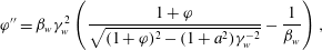 $$\begin{eqnarray}{\it\varphi}^{\prime \prime }={\it\beta}_{w}{\it\gamma}_{w}^{2}\left(\frac{1+{\it\varphi}}{\sqrt{(1+{\it\varphi})^{2}-(1+a^{2}){\it\gamma}_{w}^{-2}}}-\frac{1}{{\it\beta}_{w}}\right),\end{eqnarray}$$
where
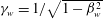 ${\it\gamma}_{w}=1/\sqrt{1-{\it\beta}_{w}^{2}}$
.
${\it\gamma}_{w}=1/\sqrt{1-{\it\beta}_{w}^{2}}$
.
We assume that the driver pulse has a constant amplitude,
 $|a|=\text{constant}$
for
$|a|=\text{constant}$
for
 $X<0$
and its amplitude is equal to zero for
$X<0$
and its amplitude is equal to zero for
 $X>0$
. Multiplying (2.8) by
$X>0$
. Multiplying (2.8) by
 ${\it\varphi}^{\prime }$
and integrating over
${\it\varphi}^{\prime }$
and integrating over
 $X$
we obtain the integral
$X$
we obtain the integral
 $$\begin{eqnarray}\frac{1}{2}({\it\varphi}^{\prime })^{2}={\it\beta}_{w}{\it\gamma}_{w}^{2}\left(\sqrt{(1+{\it\varphi})^{2}-(1+a^{2}){\it\gamma}_{w}^{-2}}-\frac{{\it\varphi}}{{\it\beta}_{w}}\right)+C.\end{eqnarray}$$
Here
 $C$
is a constant determined by the boundary conditions. If at the driver pulse front
$C$
is a constant determined by the boundary conditions. If at the driver pulse front
 $X=0$
the potential
$X=0$
the potential
 ${\it\varphi}(0)$
and the electric field,
${\it\varphi}(0)$
and the electric field,
 $E(0)=-{\it\varphi}^{\prime }(0)$
, are equal to zero, the integration constant is given by
$E(0)=-{\it\varphi}^{\prime }(0)$
, are equal to zero, the integration constant is given by
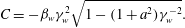 $$\begin{eqnarray}C=-{\it\beta}_{w}{\it\gamma}_{w}^{2}\sqrt{1-(1+a^{2}){\it\gamma}_{w}^{-2}}.\end{eqnarray}$$

Figure 1. Electric field and electrostatic potential of the wake wave generated (a) by a semi-infinite flat top driver pulse with the amplitude
 $a=5$
in a plasma with
$a=5$
in a plasma with
 ${\it\beta}_{w}=0.9999$
(
${\it\beta}_{w}=0.9999$
(
 ${\it\gamma}_{w}=70$
); (b) by a flat top driver pulse (indicated as
${\it\gamma}_{w}=70$
); (b) by a flat top driver pulse (indicated as
 $a(X)$
) of the optimal length
$a(X)$
) of the optimal length
 $l_{opt}$
with amplitude
$l_{opt}$
with amplitude
 $a=5$
in a plasma with
$a=5$
in a plasma with
 ${\it\beta}_{w}=1$
, (
${\it\beta}_{w}=1$
, (
 $l_{las}=10.6969$
); (c) by a wakeless driver pulse (indicated as
$l_{las}=10.6969$
); (c) by a wakeless driver pulse (indicated as
 $a(X)$
) of the double optimal length,
$a(X)$
) of the double optimal length,
 $l_{las}=2l_{opt}$
with the amplitude
$l_{las}=2l_{opt}$
with the amplitude
 $a=5$
in a plasma with
$a=5$
in a plasma with
 ${\it\beta}_{w}=1$
, (
${\it\beta}_{w}=1$
, (
 $l_{las}=21.3939$
); (d) by an ultra-short driver pulse (indicated as
$l_{las}=21.3939$
); (d) by an ultra-short driver pulse (indicated as
 $a(X)$
) with the amplitude
$a(X)$
) with the amplitude
 $a=0.5$
and length
$a=0.5$
and length
 $l_{las}=0.5$
, i.e.
$l_{las}=0.5$
, i.e.
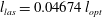 $l_{las}=0.04674\,l_{opt}$
, in a plasma with
$l_{las}=0.04674\,l_{opt}$
, in a plasma with
 ${\it\beta}_{w}=1$
.
${\it\beta}_{w}=1$
.
The electric field and electrostatic potential dependence on the coordinate
 $X$
are shown in figure 1(a), for the wake wave generated by a flat top driver pulse with amplitude
$X$
are shown in figure 1(a), for the wake wave generated by a flat top driver pulse with amplitude
 $a=5$
in a plasma with
$a=5$
in a plasma with
 ${\it\beta}_{w}=0.9999$
(
${\it\beta}_{w}=0.9999$
(
 ${\it\gamma}_{w}=70$
). The electrostatic potential has a maximum at the point where the
${\it\gamma}_{w}=70$
). The electrostatic potential has a maximum at the point where the
 ${\it\varphi}^{\prime }=0$
, i. e. where the electric field vanishes. Equations (2.9) and (2.10) yield for the maximum potential
${\it\varphi}^{\prime }=0$
, i. e. where the electric field vanishes. Equations (2.9) and (2.10) yield for the maximum potential
 $$\begin{eqnarray}{\it\varphi}_{max}=2{\it\beta}_{w}{\it\gamma}_{w}^{2}\left({\it\beta}_{w}-\sqrt{1-(1+a^{2}){\it\gamma}_{w}^{-2}}\right),\end{eqnarray}$$
which, in the limit
 $|a|\ll 1$
, is given by
$|a|\ll 1$
, is given by
 ${\it\varphi}_{max}\approx a^{2}/{\it\beta}_{w}$
and cannot exceed the value
${\it\varphi}_{max}\approx a^{2}/{\it\beta}_{w}$
and cannot exceed the value
 $2{\it\beta}_{w}^{2}{\it\gamma}_{w}^{2}$
reached for the driver laser amplitude equal to
$2{\it\beta}_{w}^{2}{\it\gamma}_{w}^{2}$
reached for the driver laser amplitude equal to
 $$\begin{eqnarray}|a|={\it\beta}_{w}{\it\gamma}_{w}.\end{eqnarray}$$
At the minimum, the electrostatic potential vanishes,
 ${\it\varphi}_{min}=0$
.
${\it\varphi}_{min}=0$
.
If the driver amplitude is above
 ${\it\beta}_{w}{\it\gamma}_{w}$
, the wake wave breaks. It cannot be described within the framework of the stationary wave approximation (see discussions of the electric field behaviour in breaking wake waves in Bulanov et al. (Reference Bulanov, Esirkepov, Kando, Koga, Pirozhkov, Nakamura, Bulanov, Schroeder, Esarey and Califano2012a
)). The electric field maximum corresponds to the extremum of the second derivative of the electrostatic potential, i.e. when the right-hand side of (2.8) vanishes. This condition gives an expression for the electrostatic potential at the electric field extremum:
${\it\beta}_{w}{\it\gamma}_{w}$
, the wake wave breaks. It cannot be described within the framework of the stationary wave approximation (see discussions of the electric field behaviour in breaking wake waves in Bulanov et al. (Reference Bulanov, Esirkepov, Kando, Koga, Pirozhkov, Nakamura, Bulanov, Schroeder, Esarey and Califano2012a
)). The electric field maximum corresponds to the extremum of the second derivative of the electrostatic potential, i.e. when the right-hand side of (2.8) vanishes. This condition gives an expression for the electrostatic potential at the electric field extremum:
 $$\begin{eqnarray}{\it\varphi}_{ex}=\pm \sqrt{1+a^{2}}-1.\end{eqnarray}$$
Substitution of this expression into (2.9) with the constant
 $C$
given by (2.10) results in
$C$
given by (2.10) results in
 $$\begin{eqnarray}|E_{m}|=\sqrt{{\it\gamma}_{w}^{2}\mp \sqrt{1+a^{2}}-{\it\beta}_{w}{\it\gamma}_{w}\sqrt{{\it\gamma}_{w}^{2}-(1+a^{2})}}.\end{eqnarray}$$
If
 $|a|\ll 1$
, the maximum electric field is proportional to the square of the driver pulse amplitude:
$|a|\ll 1$
, the maximum electric field is proportional to the square of the driver pulse amplitude:
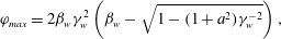
 $|E_{m}|\approx a^{2}/2{\it\beta}_{w}$
. Figure 2 shows the maximum electric field dependence on the driver pulse amplitude
$|E_{m}|\approx a^{2}/2{\it\beta}_{w}$
. Figure 2 shows the maximum electric field dependence on the driver pulse amplitude
 $a$
and the wake wave phase velocity
$a$
and the wake wave phase velocity
 ${\it\beta}_{w}$
. For a given phase velocity of the wake wave, the stationary wave can exist provided the driver amplitude is less than
${\it\beta}_{w}$
. For a given phase velocity of the wake wave, the stationary wave can exist provided the driver amplitude is less than
 $a_{lim}=\sqrt{{\it\gamma}_{w}^{2}-1}$
.
$a_{lim}=\sqrt{{\it\gamma}_{w}^{2}-1}$
.
Figure 2. Maximum electric field dependence on the driver pulse amplitude
 $a$
and the wake wave phase velocity
$a$
and the wake wave phase velocity
 ${\it\beta}_{w}$
.
${\it\beta}_{w}$
.
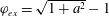
The upper limit on the electric field in a stationary wake wave inside the laser pulse corresponds to the condition given by (2.12). This yields
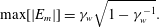 $$\begin{eqnarray}\max [|E_{m}|]={\it\gamma}_{w}\sqrt{1-{\it\gamma}_{w}^{-1}}.\end{eqnarray}$$
As for the wake wave left in a plasma the amplitude of the laser driver pulse with optimal duration cannot exceed the Akhiezer–Polovin wave breaking limit (Akhiezer & Polovin Reference Akhiezer and Polovin1956):
 $$\begin{eqnarray}|E_{A-P}|=\sqrt{2({\it\gamma}_{w}-1)}.\end{eqnarray}$$
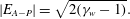
2.2 Limit
 ${\it\beta}_{w}\rightarrow 1$

In the case of a cold plasma, when the front of the driver pulse propagates with a velocity equal to the speed of light in a vacuum, which corresponds to the limit
 ${\it\beta}_{w}\rightarrow 1$
(i.e.
${\it\beta}_{w}\rightarrow 1$
(i.e.
 ${\it\gamma}_{w}\rightarrow \infty$
), (2.8) takes the form (see review article Esarey et al. (Reference Esarey, Schroeder and Leemans2009) and references therein)
${\it\gamma}_{w}\rightarrow \infty$
), (2.8) takes the form (see review article Esarey et al. (Reference Esarey, Schroeder and Leemans2009) and references therein)
 $$\begin{eqnarray}{\it\varphi}^{\prime \prime }=\frac{1}{2}\left(\frac{1+a^{2}}{(1+{\it\varphi})^{2}}-1\right).\end{eqnarray}$$
The integral (2.9), in the case of constant-amplitude driver pulse, for the boundary conditions
 ${\it\varphi}(0)=0$
and
${\it\varphi}(0)=0$
and
 ${\it\varphi}^{\prime }(0)=0$
has the form
${\it\varphi}^{\prime }(0)=0$
has the form
 $$\begin{eqnarray}({\it\varphi}^{\prime })^{2}=\frac{{\it\varphi}(a^{2}-{\it\varphi})}{1+{\it\varphi}}.\end{eqnarray}$$
We see that the electrostatic potential value varies between the minimum equal to 0 and the maximum, which equals
 ${\it\varphi}_{m}=a^{2}$
. The maximal value of the electric field is reached at the point of the electrostatic potential extremum where its second derivative vanishes. Using (2.17) we find that at the electric field maximum, the electrostatic potential is
${\it\varphi}_{m}=a^{2}$
. The maximal value of the electric field is reached at the point of the electrostatic potential extremum where its second derivative vanishes. Using (2.17) we find that at the electric field maximum, the electrostatic potential is
 ${\it\varphi}_{ex}=\sqrt{1+a^{2}}-1$
. Substituting this expression into the right-hand side of (2.18) we obtain for the electric field maximum,
${\it\varphi}_{ex}=\sqrt{1+a^{2}}-1$
. Substituting this expression into the right-hand side of (2.18) we obtain for the electric field maximum,
 $$\begin{eqnarray}|E|_{m}=\sqrt{1+a^{2}}-1.\end{eqnarray}$$
Solution of (2.17) can be expressed in terms of elliptic functions (Bulanov, Kirsanov & Sakharov Reference Bulanov, Kirsanov and Sakharov1989). The dependence of the electrostatic potential
 ${\it\varphi}$
on the coordinate
${\it\varphi}$
on the coordinate
 $X$
can be written in the implicit form:
$X$
can be written in the implicit form:
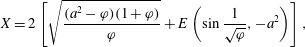 $$\begin{eqnarray}X=2\left[\sqrt{\frac{(a^{2}-{\it\varphi})(1+{\it\varphi})}{{\it\varphi}}}+E\left(\sin \frac{1}{\sqrt{{\it\varphi}}},-a^{2}\right)\right],\end{eqnarray}$$
where
 $E({\it\phi},k)$
is the elliptic integral of the second kind (Gradshteyn & Ryzhik Reference Gradshteyn and Ryzhik1980).
$E({\it\phi},k)$
is the elliptic integral of the second kind (Gradshteyn & Ryzhik Reference Gradshteyn and Ryzhik1980).
2.3 Optimal length of the laser pulse
The laser pulse is optimal for the excitation of the large-amplitude wake field left behind it, if at the rear side of the the electrostatic potential is maximal. From (2.18) follows the expression for the optimal pulse length,
 $l_{opt}$
:
$l_{opt}$
:
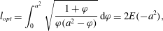 $$\begin{eqnarray}l_{opt}=\int _{0}^{a^{2}}\sqrt{\frac{1+{\it\varphi}}{{\it\varphi}(a^{2}-{\it\varphi})}}\,\text{d}{\it\varphi}=2E(-a^{2}),\end{eqnarray}$$
where
 $E(k)$
is the complete elliptic integral of the second kind (Gradshteyn & Ryzhik Reference Gradshteyn and Ryzhik1980).
$E(k)$
is the complete elliptic integral of the second kind (Gradshteyn & Ryzhik Reference Gradshteyn and Ryzhik1980).
The wake wave wavelength equals
 ${\it\lambda}_{w}=4l_{opt}$
in the limit of small laser amplitude
${\it\lambda}_{w}=4l_{opt}$
in the limit of small laser amplitude
 $a\ll 1$
and it is approximately
$a\ll 1$
and it is approximately
 $2l_{opt}$
for
$2l_{opt}$
for
 $a\gg 1$
.
$a\gg 1$
.
In the small-amplitude limit,
 $|a|\ll 1$
, the optimal laser length is
$|a|\ll 1$
, the optimal laser length is
 $$\begin{eqnarray}l_{opt}={\rm\pi}+\frac{{\rm\pi}}{4}a^{2}-\frac{3{\rm\pi}}{64}a^{4}+O[a^{2}]^{3},\end{eqnarray}$$
and the wake wave wavelength in dimensional units equals
 ${\it\lambda}_{w}=2{\rm\pi}c/{\it\omega}_{pe}$
. If the driver amplitude equals unity,
${\it\lambda}_{w}=2{\rm\pi}c/{\it\omega}_{pe}$
. If the driver amplitude equals unity,
 $|a|=1$
, the optimal laser length is 3.8202. For large laser amplitude,
$|a|=1$
, the optimal laser length is 3.8202. For large laser amplitude,
 $a^{2}\gg 1$
, we have
$a^{2}\gg 1$
, we have
 $$\begin{eqnarray}l_{opt}=2|a|+\left(\frac{1}{2}+2\ln 2-\ln |a|\right)\frac{1}{|a|}+O\left[\frac{1}{|a|}\right]^{3}\end{eqnarray}$$
with the wake wave wavelength in dimensional units equal to
 ${\it\lambda}_{w}=4c|a|/{\it\omega}_{pe}$
. In figure 2 we plot the dependence of the optimal laser length on the pulse amplitude.
${\it\lambda}_{w}=4c|a|/{\it\omega}_{pe}$
. In figure 2 we plot the dependence of the optimal laser length on the pulse amplitude.
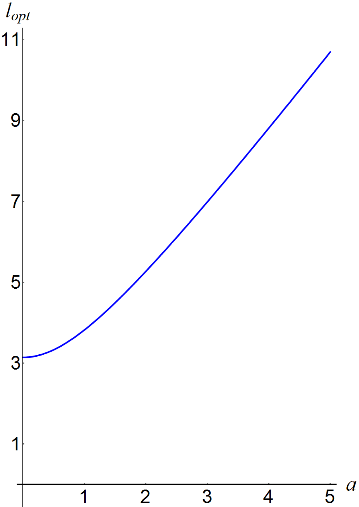
Figure 3. Optimal laser length
 $l_{opt}$
versus the pulse amplitude
$l_{opt}$
versus the pulse amplitude
 $a$
.
$a$
.
The electric field and electrostatic potential dependence on the coordinate
 $X$
are shown in figure 1(b), for the wake wave generated by a flat top driver pulse of the optimal length
$X$
are shown in figure 1(b), for the wake wave generated by a flat top driver pulse of the optimal length
 $l_{opt}$
. The amplitude is
$l_{opt}$
. The amplitude is
 $a=5$
. Equation (2.21) for this laser amplitude gives
$a=5$
. Equation (2.21) for this laser amplitude gives
 $l_{opt}=10.6969$
. The plasma is characterized by
$l_{opt}=10.6969$
. The plasma is characterized by
 ${\it\beta}_{w}=1$
(
${\it\beta}_{w}=1$
(
 ${\it\gamma}_{w}=70$
).
${\it\gamma}_{w}=70$
).
The wake wave left behind the driver laser pulse is described by (2.17) with
 $a^{2}=0$
. For the boundary conditions
$a^{2}=0$
. For the boundary conditions
 ${\it\varphi}(-l_{opt})=a^{2}$
and
${\it\varphi}(-l_{opt})=a^{2}$
and
 ${\it\varphi}^{\prime }(-l_{opt})=0$
the equation for the electric field,
${\it\varphi}^{\prime }(-l_{opt})=0$
the equation for the electric field,
 $E=-{\it\varphi}^{\prime }$
, reads
$E=-{\it\varphi}^{\prime }$
, reads
 $$\begin{eqnarray}E^{2}=a^{2}-{\it\varphi}-\frac{a^{2}-{\it\varphi}}{(1+a^{2})(1+{\it\varphi})}.\end{eqnarray}$$
From this equation it follows that the electrostatic potential in the wake wave varies between maximal and minimal values at the points where
 $E=-{\it\varphi}^{\prime }=0$
:
$E=-{\it\varphi}^{\prime }=0$
:
 $$\begin{eqnarray}-\frac{a^{2}}{1+a^{2}}<{\it\varphi}<a^{2}.\end{eqnarray}$$
The electric field maximum is determined by the condition
 ${\it\varphi}^{\prime \prime }=0$
, which gives the extremum of the electrostatic potential derivative reached at the points where
${\it\varphi}^{\prime \prime }=0$
, which gives the extremum of the electrostatic potential derivative reached at the points where
 ${\it\varphi}=0$
. From (2.24) it follows that the electric field maximum equals (see also Esarey et al.
Reference Esarey, Schroeder and Leemans2009)
${\it\varphi}=0$
. From (2.24) it follows that the electric field maximum equals (see also Esarey et al.
Reference Esarey, Schroeder and Leemans2009)
 $$\begin{eqnarray}E_{m}=\frac{a^{2}}{\sqrt{1+a^{2}}}.\end{eqnarray}$$
It is larger than the maximum of the wake field inside the driver laser pulse given by (2.19), as also seen in figure 1(b).
If the laser pulse has double the optimal length,
 $l_{las}=2l_{opt}$
, then the wake wave left behind the laser pulse vanishes with the electric field and electrostatic potential localized only inside the laser pulse, as illustrated in figure 1(c), where the electric field and electrostatic potential of the wake wave generated by a wakeless driver pulse (indicated as
$l_{las}=2l_{opt}$
, then the wake wave left behind the laser pulse vanishes with the electric field and electrostatic potential localized only inside the laser pulse, as illustrated in figure 1(c), where the electric field and electrostatic potential of the wake wave generated by a wakeless driver pulse (indicated as
 $a(X)$
) of double the optimal length,
$a(X)$
) of double the optimal length,
 $l_{las}=2l_{opt}$
with amplitude
$l_{las}=2l_{opt}$
with amplitude
 $a=5$
in a plasma with
$a=5$
in a plasma with
 ${\it\beta}_{w}=1$
are shown as functions of the coordinate
${\it\beta}_{w}=1$
are shown as functions of the coordinate
 $X$
.
$X$
.
Formally, a laser pulse of double the optimal length does not lose energy in the wake wave generation because the energy lost at the front returns back at the rear side of the pulse. Actually, the laser pulse etching (see consideration of this effect in § 2.5 below) and the laser pulse self-modulation (Andreev et al. Reference Andreev, Gorbunov, Kirsanov, Pogosova and Ramazashvili1992; Antonsen & Mora Reference Antonsen and Mora1992; Sprangle et al. Reference Sprangle, Esarey, Krall and Joyce1992; Bulanov et al. Reference Bulanov, Esirkepov, Naumova, Pegoraro, Pogorelsky and Pukhov1996) will result in a change of the laser pulse length, amplitude and form, eventually leading to the appearance of a final amplitude wake wave in the plasma behind the laser pulse and to laser pulse energy depletion.
2.4 Wake wave excitation by the ultra-short laser pulse
In the case when the laser pulse length
 $l_{las}$
is substantially shorter than the optimal length given by (2.21), the electric field and the electrostatic potential at the rear end of the pulse can be found from (2.17). They are equal to
$l_{las}$
is substantially shorter than the optimal length given by (2.21), the electric field and the electrostatic potential at the rear end of the pulse can be found from (2.17). They are equal to
 $$\begin{eqnarray}E_{1}=\frac{l_{las}}{2}a^{2}\end{eqnarray}$$
and
 $$\begin{eqnarray}{\it\varphi}_{1}=\frac{l_{las}^{2}}{4}a^{2},\end{eqnarray}$$
respectively. The wake wave wavelength, in this case, is equal to
 $$\begin{eqnarray}{\it\lambda}_{w,1}=2l_{las}a^{2}.\end{eqnarray}$$
The electric field and electrostatic potential dependence on the coordinate
 $X$
are shown in figure 1(d), for the wake wave generated by an ultra-short driver pulse with the length and amplitude equal to
$X$
are shown in figure 1(d), for the wake wave generated by an ultra-short driver pulse with the length and amplitude equal to
 $l_{las}=0.25$
and
$l_{las}=0.25$
and
 $a=5$
, respectively, in a plasma with
$a=5$
, respectively, in a plasma with
 ${\it\beta}_{w}=0.9999$
(
${\it\beta}_{w}=0.9999$
(
 ${\it\gamma}_{w}=70$
).
${\it\gamma}_{w}=70$
).
The electrostatic potential has a maximum at the point where
 ${\it\varphi}^{\prime }=0$
, i.e. where the electric field vanishes. Equation (2.9) yields the equation determining the potential maximum and the minimum
${\it\varphi}^{\prime }=0$
, i.e. where the electric field vanishes. Equation (2.9) yields the equation determining the potential maximum and the minimum
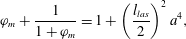 $$\begin{eqnarray}{\it\varphi}_{m}+\frac{1}{1+{\it\varphi}_{m}}=1+\left(\frac{l_{las}}{2}\right)^{2}a^{4},\end{eqnarray}$$
which has the solution:
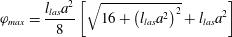 $$\begin{eqnarray}{\it\varphi}_{max}=\frac{l_{las}a^{2}}{8}\left[\sqrt{16+\left(l_{las}a^{2}\right)^{2}}+l_{las}a^{2}\right]\end{eqnarray}$$
for the electrostatic potential maximum and
 $$\begin{eqnarray}{\it\varphi}_{min}=-\frac{l_{las}a^{2}}{8}\left[\sqrt{16+\left(l_{las}a^{2}\right)^{2}}-l_{las}a^{2}\right]\end{eqnarray}$$
for the minimum, respectively.
In the limit
 $(l_{las}/2)a^{2}\ll 1$
, we find
$(l_{las}/2)a^{2}\ll 1$
, we find
 ${\it\varphi}_{max}\approx (l_{las}/2)a^{2}$
. The electric field in the wake wave is approximately equal to
${\it\varphi}_{max}\approx (l_{las}/2)a^{2}$
. The electric field in the wake wave is approximately equal to
 $E_{1}$
given by (2.27). If
$E_{1}$
given by (2.27). If
 $(l_{las}/2)a^{2}\gg 1$
the maximum potential is approximately equal to
$(l_{las}/2)a^{2}\gg 1$
the maximum potential is approximately equal to
 $(l_{las}/2)^{2}a^{4}$
. For minimum value of the electrostatic potential we have
$(l_{las}/2)^{2}a^{4}$
. For minimum value of the electrostatic potential we have
 ${\it\varphi}_{min}\approx -(l_{las}/2)a^{2}$
in the limit of relatively small laser amplitude,
${\it\varphi}_{min}\approx -(l_{las}/2)a^{2}$
in the limit of relatively small laser amplitude,
 $(l_{las}/2)a^{2}\ll 1$
, and it is equal to
$(l_{las}/2)a^{2}\ll 1$
, and it is equal to
 $-1$
for substantially high laser amplitude,
$-1$
for substantially high laser amplitude,
 $(l_{las}/2)a^{2}\gg 1$
, respectively.
$(l_{las}/2)a^{2}\gg 1$
, respectively.
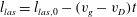
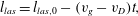
2.5 Propagation velocity of the laser pulse front
In the expressions obtained above the phase velocity of the wake wave,
 ${\it\beta}_{w}$
, is equal to the propagation velocity of the laser pulse front. Apart from its dependence on the group velocity of the electromagnetic wave determined by the plasma density, it is also determined by the process of laser pulse energy depletion, which results in the change of the laser pulse form manifesting itself in the formation of a shock-wave-like front and in carrier frequency down shift. These phenomena have been discussed by Bulanov et al. (Reference Bulanov, Inovenkov, Kirsanov, Naumova and Sakharov1992, Reference Bulanov, Kirsanov, Naumova, Sakharov, Shah and Inovenkov1993), Decker et al. (Reference Decker, Mori, Tzeng and Katsouleas1996), Lu et al. (Reference Lu, Tzoufras, Joshi, Tsung, Mori, Vieira, Fonseca and Silva2007), Schroeder et al. (Reference Schroeder, Benedetti, Esarey, Grüner and Leemans2011), Bulanov et al. (Reference Bulanov, Esarey, Schroeder, Bulanov, Esirkepov, Kando, Pegoraro and Leemans2015). The laser energy depletion associated with the so-called etching (Nakajima et al.
Reference Nakajima, Deng, Zhang, Shen, Liu, Li, Xu, Ostermayr, Petrovics and Klier2011) of the pulse, makes the pulse front velocity
${\it\beta}_{w}$
, is equal to the propagation velocity of the laser pulse front. Apart from its dependence on the group velocity of the electromagnetic wave determined by the plasma density, it is also determined by the process of laser pulse energy depletion, which results in the change of the laser pulse form manifesting itself in the formation of a shock-wave-like front and in carrier frequency down shift. These phenomena have been discussed by Bulanov et al. (Reference Bulanov, Inovenkov, Kirsanov, Naumova and Sakharov1992, Reference Bulanov, Kirsanov, Naumova, Sakharov, Shah and Inovenkov1993), Decker et al. (Reference Decker, Mori, Tzeng and Katsouleas1996), Lu et al. (Reference Lu, Tzoufras, Joshi, Tsung, Mori, Vieira, Fonseca and Silva2007), Schroeder et al. (Reference Schroeder, Benedetti, Esarey, Grüner and Leemans2011), Bulanov et al. (Reference Bulanov, Esarey, Schroeder, Bulanov, Esirkepov, Kando, Pegoraro and Leemans2015). The laser energy depletion associated with the so-called etching (Nakajima et al.
Reference Nakajima, Deng, Zhang, Shen, Liu, Li, Xu, Ostermayr, Petrovics and Klier2011) of the pulse, makes the pulse front velocity
 ${\it\beta}_{D}$
become smaller than the group velocity of the laser radiation
${\it\beta}_{D}$
become smaller than the group velocity of the laser radiation
 ${\it\beta}_{g}$
. This process is illustrated in figure 4.
${\it\beta}_{g}$
. This process is illustrated in figure 4.
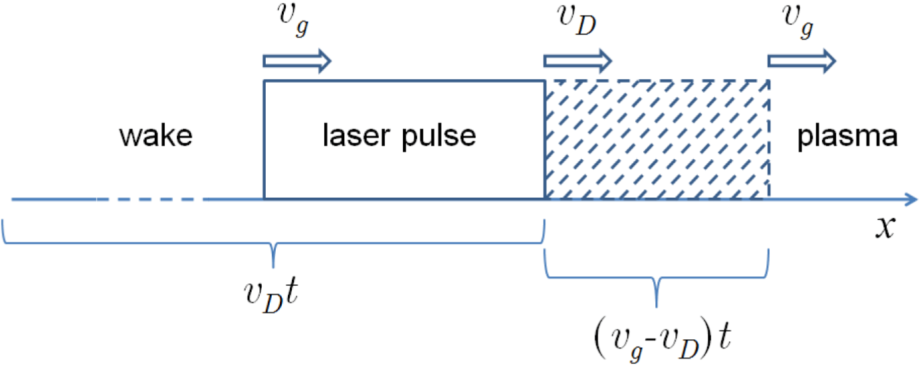
Figure 4. The laser energy depletion leads to the laser pulse shortening
 $l_{las}=l_{las,0}-(v_{g}-v_{D})t$
and to slower propagation of the pulse front with velocity
$l_{las}=l_{las,0}-(v_{g}-v_{D})t$
and to slower propagation of the pulse front with velocity
 $v_{D}<v_{g}$
. The shaded region shows the damped part of the pulse.
$v_{D}<v_{g}$
. The shaded region shows the damped part of the pulse.
In order to find the laser pulse front velocity we should take into account the balance between the lost laser energy
 $$\begin{eqnarray}\frac{m_{e}^{2}{\it\omega}^{2}c^{2}a^{2}}{4e^{2}{\rm\pi}}(v_{g}-v_{D})t\end{eqnarray}$$
and the wake wave energy
 $$\begin{eqnarray}m_{e}c^{2}na^{2}v_{D}t.\end{eqnarray}$$
This gives the relationship between the group velocity of the laser pulse and the velocity of propagation of the pulse front, which in normalized units reads:
 $$\begin{eqnarray}{\it\beta}_{D}=\frac{{\it\beta}_{g}}{1+({\it\omega}_{pe}/{\it\omega})^{2}}.\end{eqnarray}$$
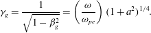
Here, a 1-D geometry is assumed; the 3-D scaling has been found in Bulanov et al. (Reference Bulanov, Esarey, Schroeder, Bulanov, Esirkepov, Kando, Pegoraro and Leemans2015). The group velocity
 ${\it\beta}_{g}$
of the relativistically intense electromagnetic wave according to Akhiezer & Polovin (Reference Akhiezer and Polovin1956) depends on its amplitude: associated with the group velocity Lorentz factor in the case of a circularly polarized wave
${\it\beta}_{g}$
of the relativistically intense electromagnetic wave according to Akhiezer & Polovin (Reference Akhiezer and Polovin1956) depends on its amplitude: associated with the group velocity Lorentz factor in the case of a circularly polarized wave
 $$\begin{eqnarray}{\it\gamma}_{g}=\frac{1}{\sqrt{1-{\it\beta}_{g}^{2}}}=\left(\frac{{\it\omega}}{{\it\omega}_{pe}}\right)(1+a^{2})^{1/4}.\end{eqnarray}$$
In the limit
 $|a|\gg 1$
it is proportional to the square root of the wave amplitude. This dependence has important implications for determining the wake wave breaking threshold (Zhidkov et al.
Reference Zhidkov, Koga, Kinoshita and Uesaka2004a
,Reference Zhidkov, Koga, Hosokai, Kinoshita and Uesaka
b
), which in its turn determines the threshold of electron self-injection to the wake field. Due to laser energy depletion the laser pulse length decreases as
$|a|\gg 1$
it is proportional to the square root of the wave amplitude. This dependence has important implications for determining the wake wave breaking threshold (Zhidkov et al.
Reference Zhidkov, Koga, Kinoshita and Uesaka2004a
,Reference Zhidkov, Koga, Hosokai, Kinoshita and Uesaka
b
), which in its turn determines the threshold of electron self-injection to the wake field. Due to laser energy depletion the laser pulse length decreases as
 $$\begin{eqnarray}l_{las}=l_{las,0}-(v_{g}-v_{D})t,\end{eqnarray}$$
where
 $l_{las,0}$
is the initial pulse length. From this expression and (2.35), (2.36) follows that the depletion length is equal to (for details see Bulanov et al. (Reference Bulanov, Inovenkov, Kirsanov, Naumova and Sakharov1992), Decker et al. (Reference Decker, Mori, Tzeng and Katsouleas1996))
$l_{las,0}$
is the initial pulse length. From this expression and (2.35), (2.36) follows that the depletion length is equal to (for details see Bulanov et al. (Reference Bulanov, Inovenkov, Kirsanov, Naumova and Sakharov1992), Decker et al. (Reference Decker, Mori, Tzeng and Katsouleas1996))
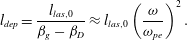 $$\begin{eqnarray}l_{dep}=\frac{l_{las,0}}{{\it\beta}_{g}-{\it\beta}_{D}}\approx l_{las,0}\left(\frac{{\it\omega}}{{\it\omega}_{pe}}\right)^{2}.\end{eqnarray}$$
We note that the laser pulse with the length
 $l_{las,0}$
substantially larger than the wavelength of the wake wave is unstable against various instabilities. As a result the self-modulated wake wave regime occurs (Andreev et al.
Reference Andreev, Gorbunov, Kirsanov, Pogosova and Ramazashvili1992; Antonsen & Mora Reference Antonsen and Mora1992; Sprangle et al.
Reference Sprangle, Esarey, Krall and Joyce1992), which has been studied in experiments on short, but not too short, laser pulse interaction with underdense plasma targets (Hidding et al.
Reference Hidding, Amthor, Liesfeld, Schwoerer, Karsch, Geissler, Veisz, Schmid, Gallacher and Jamison2006; Mori et al.
Reference Mori, Kando, Daito, Kotaki, Hayashi, Yamazaki, Ogura, Sagisaka, Koga and Nakajima2006). In the self-modulated wake-field regime, the depletion length is shorter than the length given by expression (2.38), in which we should instead of
$l_{las,0}$
substantially larger than the wavelength of the wake wave is unstable against various instabilities. As a result the self-modulated wake wave regime occurs (Andreev et al.
Reference Andreev, Gorbunov, Kirsanov, Pogosova and Ramazashvili1992; Antonsen & Mora Reference Antonsen and Mora1992; Sprangle et al.
Reference Sprangle, Esarey, Krall and Joyce1992), which has been studied in experiments on short, but not too short, laser pulse interaction with underdense plasma targets (Hidding et al.
Reference Hidding, Amthor, Liesfeld, Schwoerer, Karsch, Geissler, Veisz, Schmid, Gallacher and Jamison2006; Mori et al.
Reference Mori, Kando, Daito, Kotaki, Hayashi, Yamazaki, Ogura, Sagisaka, Koga and Nakajima2006). In the self-modulated wake-field regime, the depletion length is shorter than the length given by expression (2.38), in which we should instead of
 $l_{las,0}$
use the wavelength of the wake wave
$l_{las,0}$
use the wavelength of the wake wave
 ${\approx}4E(-a^{2})$
(see (2.21)).
${\approx}4E(-a^{2})$
(see (2.21)).
The energy depletion length of the laser pulse of the short length exciting the wake wave electrostatic potential according to (2.31) is
 $$\begin{eqnarray}l_{dep}=\frac{8c^{2}{\it\omega}^{2}}{{\it\omega}_{pe}^{3}\left[l_{las}{\it\omega}_{pe}a^{2}+\sqrt{16c^{2}+\left(l_{las}{\it\omega}_{pe}a^{2}\right)^{2}}\right]}.\end{eqnarray}$$
It is written in dimensional units.
In the limit
 $l_{las}{\it\omega}_{pe}a^{2}/2c\ll 1$
, the depletion length
$l_{las}{\it\omega}_{pe}a^{2}/2c\ll 1$
, the depletion length
 $$\begin{eqnarray}l_{dep}=\frac{2c}{{\it\omega}_{pe}}\left(\frac{{\it\omega}}{{\it\omega}_{pe}}\right)^{2}\end{eqnarray}$$
neither depends on the laser pulse amplitude nor length.
When
 $l_{las}{\it\omega}_{pe}a^{2}/2c\gg 1$
the depletion length
$l_{las}{\it\omega}_{pe}a^{2}/2c\gg 1$
the depletion length
 $$\begin{eqnarray}l_{dep}=4l_{las}\left(\frac{c}{a{\it\omega}_{pe}l_{las}}\right)^{2}\left(\frac{{\it\omega}}{{\it\omega}_{pe}}\right)^{2}\end{eqnarray}$$
is inversely proportional to the laser pulse length,
 $l_{dep}\propto 1/l_{las}$
.
$l_{dep}\propto 1/l_{las}$
.
2.6 Wake wave generation by chirped laser pulse driver
As has been shown in Deutsch, Meerson & Golub (Reference Deutsch, Meerson and Golub1991), Khachatryan et al. (Reference Khachatryan, van Goor, Verschuur and Boller2005), Kalmykov et al. (Reference Kalmykov, Beck, Davoine, Lefebvre and Shadwick2012), the use of the frequency modulated laser pulse (chirped pulse driver) can improve the quality of the wake wave generated in plasmas. A properly chosen chirp can compensate the frequency downshift effect on the front of the laser pulse (see discussion of this effect in Bulanov et al. (Reference Bulanov, Inovenkov, Kirsanov, Naumova and Sakharov1992, Reference Bulanov, Kirsanov, Naumova, Sakharov, Shah and Inovenkov1993), Decker et al. (Reference Decker, Mori, Tzeng and Katsouleas1996)) thus mitigating consequences of dark current formation. Here we would like to draw attention to the fact that the chirped laser pulse propagating through a low-density plasma changes its length. The pulse stretches for the negative chirp, when the frequency monotonically changes being higher at the laser pulse front than at the rear pulse side. In the case of the positive chirp, when the frequency is lower at the front than at the rear side of the laser pulse, the pulse shrinks.
As an example, we consider the laser pulse dependence on coordinate and time given by the formula
 $$\begin{eqnarray}a(t,x)=|a(t,x)|\exp \left(-\text{i}({\it\omega}_{0}t-k_{0}x+{\it\theta}(t,x))\right),\end{eqnarray}$$
where
 ${\it\omega}_{0}$
and
${\it\omega}_{0}$
and
 $k_{0}$
are, respectively, the high carrier frequency and wavenumber, related to each other by the dispersion equation
$k_{0}$
are, respectively, the high carrier frequency and wavenumber, related to each other by the dispersion equation
 ${\it\omega}_{0}=\sqrt{k_{0}^{2}c^{2}+{\it\omega}_{pe}^{2}}$
. Dependence of the phase shift
${\it\omega}_{0}=\sqrt{k_{0}^{2}c^{2}+{\it\omega}_{pe}^{2}}$
. Dependence of the phase shift
 ${\it\theta}(t,x)$
on time and coordinate describes the chirp.
${\it\theta}(t,x)$
on time and coordinate describes the chirp.
The laser pulse evolution within the framework of the approximation of slowly varying amplitude
 $|a({\it\tau},{\it\zeta})|$
and phase
$|a({\it\tau},{\it\zeta})|$
and phase
 ${\it\theta}({\it\tau},{\it\zeta})$
can be described by (5) obtained by Bulanov et al. (Reference Bulanov, Inovenkov, Kirsanov, Naumova and Sakharov1992) or (80) from Esarey et al. (Reference Esarey, Schroeder and Leemans2009). Here we use normalized variables
${\it\theta}({\it\tau},{\it\zeta})$
can be described by (5) obtained by Bulanov et al. (Reference Bulanov, Inovenkov, Kirsanov, Naumova and Sakharov1992) or (80) from Esarey et al. (Reference Esarey, Schroeder and Leemans2009). Here we use normalized variables
 ${\it\tau}={\it\omega}_{0}t$
and
${\it\tau}={\it\omega}_{0}t$
and
 ${\it\zeta}=k_{0}x-{\it\omega}_{0}t$
. Assuming the that the time scale of the laser pulse shrinking/stretching,
${\it\zeta}=k_{0}x-{\it\omega}_{0}t$
. Assuming the that the time scale of the laser pulse shrinking/stretching,
 $t_{s}$
, is substantially shorter than the laser pulse energy depletion time (see discussion above and expressions given by (2.39)–(2.41)), we can easily find that in the self-similar evolution regime the laser pulse phase and amplitude dependence on the time
$t_{s}$
, is substantially shorter than the laser pulse energy depletion time (see discussion above and expressions given by (2.39)–(2.41)), we can easily find that in the self-similar evolution regime the laser pulse phase and amplitude dependence on the time
 ${\it\tau}$
and coordinate
${\it\tau}$
and coordinate
 ${\it\zeta}$
are given by
${\it\zeta}$
are given by
 $$\begin{eqnarray}{\it\theta}({\it\tau},{\it\zeta})=\frac{{\it\zeta}^{2}}{2(k_{0}l_{0})^{2}s({\it\tau})},\end{eqnarray}$$
and
 $$\begin{eqnarray}|a({\it\tau},{\it\zeta})|=|a(0,0)|\sqrt{\frac{1}{s({\it\tau})}\left(1-\frac{{\it\zeta}^{2}}{(k_{0}l_{0}s({\it\tau}))^{2}}\right)},\end{eqnarray}$$
respectively. Here the function
 $s({\it\tau})$
depends on time as
$s({\it\tau})$
depends on time as
 $$\begin{eqnarray}s({\it\tau})=1\mp \frac{2{\it\omega}_{pe}^{2}{\it\tau}}{{\it\omega}_{0}^{2}(k_{0}l_{0})^{2}}\end{eqnarray}$$
with
 $|a(0,0)|$
and
$|a(0,0)|$
and
 $l_{0}$
being the laser pulse amplitude and half-width, respectively, at
$l_{0}$
being the laser pulse amplitude and half-width, respectively, at
 ${\it\tau}=0$
. The sign
${\it\tau}=0$
. The sign
 $\mp$
corresponds to positive (minus) and negative (plus) chirp. The laser pulse is localized between the points
$\mp$
corresponds to positive (minus) and negative (plus) chirp. The laser pulse is localized between the points
 ${\it\zeta}=\pm s({\it\tau})(k_{0}l_{0})$
. Its width increases or decreases according to expression (2.45) for positive or negative chirp, but the pulse energy proportional to
${\it\zeta}=\pm s({\it\tau})(k_{0}l_{0})$
. Its width increases or decreases according to expression (2.45) for positive or negative chirp, but the pulse energy proportional to
 $$\begin{eqnarray}\int _{-s({\it\tau})k_{0}l_{0}}^{s({\it\tau})k_{0}l_{0}}|a({\it\tau},{\it\zeta})|^{2}\,\text{d}{\it\zeta}=\frac{5}{3}|a(0,0)|^{2}k_{0}l_{0}\end{eqnarray}$$
remains constant. The time scale of the laser pulse shrinking/stretching equals
 $$\begin{eqnarray}t_{s}=\frac{(k_{0}l_{0})^{2}}{2{\it\omega}_{0}}\left(\frac{{\it\omega}_{0}}{{\it\omega}_{pe}}\right)^{2}.\end{eqnarray}$$
As follows from (2.27) and (2.29) the electric field amplitude and the wake wave wavelength excited by an ultra-short laser pulse do not change during evolution of the chirped pulse provided its length is substantially less than the optimal pulse length given by (2.21).
When the laser pulse length approaches the optimal length the wake field amplitude can either increase or decrease depending on the laser pulse and plasma parameters. The wake-field amplitude according to (2.27) is determined by the short pulse laser energy, (we introduce the notation
 ${\it\varepsilon}_{las}=|a|^{2}l_{las}$
), i.e.
${\it\varepsilon}_{las}=|a|^{2}l_{las}$
), i.e.
 $E_{m}={\it\varepsilon}_{las}$
in the limit
$E_{m}={\it\varepsilon}_{las}$
in the limit
 $l_{las}\ll l_{opt}$
. Assuming that
$l_{las}\ll l_{opt}$
. Assuming that
 $|a|\gg 1$
, we can present the wake-field amplitude in the case of the optimal length pulse (2.26) as
$|a|\gg 1$
, we can present the wake-field amplitude in the case of the optimal length pulse (2.26) as
 $E_{m}=({\it\varepsilon}_{las}/2)^{1/3}$
for
$E_{m}=({\it\varepsilon}_{las}/2)^{1/3}$
for
 $l_{las}\approx l_{opt}$
. These two values become equal to each other for
$l_{las}\approx l_{opt}$
. These two values become equal to each other for
 ${\it\varepsilon}_{las}=1/\sqrt{2}$
. In dimensional form this condition can be rewritten as a relationship between the laser intensity
${\it\varepsilon}_{las}=1/\sqrt{2}$
. In dimensional form this condition can be rewritten as a relationship between the laser intensity
 $I$
and the plasma density
$I$
and the plasma density
 $n_{e}$
,
$n_{e}$
,
 $$\begin{eqnarray}I=5.6\times 10^{18}\left(\frac{n_{cr}}{n_{e}}\right)^{1/2}\left(\frac{1~{\rm\mu}\text{m}}{l_{las}}\right)\left(\frac{{\it\lambda}_{0}}{1~{\rm\mu}\text{m}}\right)^{3}\frac{\text{W}}{\text{cm}^{2}}.\end{eqnarray}$$
As a result, assuming the plasma density is given, for the intensity higher than that given by (2.48) the laser chirp can enhance the wake wave amplitude.
3 Electron wake-field acceleration: trapping and injection
3.1 Electron trapping into a wake wave
In the laser wake-field accelerator concept introduced in Tajima & Dawson (Reference Tajima and Dawson1979), a long-lived wake-field, induced by a short intense laser pulse in its wake in a low-density collisionless plasma, accelerates duly injected electrons. To provide electrons, one must use an externally preaccelerated electron bunch or exploit the effect of self-injection due to a longitudinal Langmuir wave break in homogeneous (Bulanov, Kirsanov & Sakharov Reference Bulanov, Kirsanov and Sakharov1991; Bulanov et al. Reference Bulanov, Inovenkov, Kirsanov, Naumova and Sakharov1992; Coverdale et al. Reference Coverdale, Darrow, Decker, Mori, Tzeng, Marsh, Clayton and Joshi1995; Gordon et al. Reference Gordon, Tzeng, Clayton, Dangor, Malka, Marsh, Modena, Mori, Muggli and Najmudin1998; Zhidkov et al. Reference Zhidkov, Koga, Kinoshita and Uesaka2004a ; Ohkubo et al. Reference Ohkubo, Bulanov, Zhidkov, Esirkepov, Koga, Uesaka and Tajima2006) and/or inhomogeneous plasma targets (Bulanov et al. Reference Bulanov, Naumova, Pegoraro and Sakai1998; Suk et al. Reference Suk, Barov, Rosenzweig and Esarey2001; Thompson et al. Reference Thompson, Rosenzweig and Suk2004; Tomassini et al. Reference Tomassini, Galimberti, Giulietti, Giulietti, Gizzi, Labate and Pegoraro2004; Brantov et al. Reference Brantov, Kando, Kotaki, Yu and Bulanov2008; Geddes et al. Reference Geddes, Nakamura, Plateau, Toth, Cormier-Michel, Esarey, Schroeder, Cary and Leemans2008; Buck et al. Reference Buck, Wenz, Xu, Khrennikov, Schmid, Heigoldt, Mikhailova, Geissler, Shen and Krausz2013; Corde et al. Reference Corde, Thaury, Lifschitz, Lambert, Ta Phuoc, Davoine, Lehe, Douillet, Rousse and Malka2013) and/or a transverse wave break (Bulanov et al. Reference Bulanov, Pegoraro, Pukhov and Sakharov1997a ; Liseikina et al. Reference Liseikina, Califano, Vshivkov, Pegoraro and Bulanov1999; Pukhov & Meyer-ter Vehn Reference Pukhov and Meyer-ter Vehn2002; Kando et al. Reference Kando, Fukuda, Kotaki, Koga, Bulanov, Tajima, Chao, Pitthan, Schuler and Zhidkov2007; Corde et al. Reference Corde, Thaury, Lifschitz, Lambert, Ta Phuoc, Davoine, Lehe, Douillet, Rousse and Malka2013). The optical injection mechanism can also provide preaccelerated electron beams with the required properties (Esarey et al. Reference Esarey, Hubbard, Leemans, Ting and Sprangle1997; Kotaki et al. Reference Kotaki, Masuda, Kando, Koga and Nakajima2004; Faure et al. Reference Faure, Rechatin, Norlin, Lifschitz, Glinec and Malka2006; Kotaki et al. Reference Kotaki, Daito, Kando, Hayashi, Kawase, Kameshima, Fukuda, Homma, Ma and Chen2009; Rechatin et al. Reference Rechatin, Faure, Ben-Ismail, Lim, Fitour, Specka, Videau, Tafzi, Burgy and Malka2009b ). The two-colour ionization injection scheme (Schroeder et al. Reference Schroeder, Benedetti, Bulanov, Chen, Esarey, Geddes, Vay, Yu and Leemans2015) and an external static magnetic field (Hosokai et al. Reference Hosokai, Kinoshita, Zhidkov, Maekawa, Yamazaki and Uesaka2006b ) enable the control of the properties of the injected/accelerated electron beams.
Electrons immersed in the wake field oscillate in a regular way. In a plasma with the electron density well below the critical one
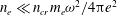 $n_{e}\ll n_{cr}m_{e}{\it\omega}^{2}/4{\rm\pi}e^{2}$
, the wake wave phase velocity
$n_{e}\ll n_{cr}m_{e}{\it\omega}^{2}/4{\rm\pi}e^{2}$
, the wake wave phase velocity
 $v_{w}=c{\it\beta}_{w}$
is close to the speed of light in a vacuum, which corresponds to a large value of the relativistic Lorentz factor,
$v_{w}=c{\it\beta}_{w}$
is close to the speed of light in a vacuum, which corresponds to a large value of the relativistic Lorentz factor,
 ${\it\gamma}_{w}$
. The group velocity of the wake wave is equal to zero and the phase velocity
${\it\gamma}_{w}$
. The group velocity of the wake wave is equal to zero and the phase velocity
 $v_{w}$
is equal to the velocity at which the laser pulse front propagates. This is given by (2.35). From these expressions, it is easy to obtain a relation between the electromagnetic pulse wavelength
$v_{w}$
is equal to the velocity at which the laser pulse front propagates. This is given by (2.35). From these expressions, it is easy to obtain a relation between the electromagnetic pulse wavelength
 ${\it\lambda}_{0}$
and the wavelength
${\it\lambda}_{0}$
and the wavelength
 ${\it\lambda}_{w}$
of the wake field:
${\it\lambda}_{w}$
of the wake field:
 $$\begin{eqnarray}{\it\lambda}_{w}={\it\lambda}_{0}\frac{\sqrt{{\it\gamma}_{w}}E(-a^{2})}{{\rm\pi}}.\end{eqnarray}$$
Assuming that the characteristic change in the electron density in the wake wave is of the order of the plasma density and considering the weakly nonlinear wave that is of interest to the discussed concept of a laser electron–positron collider (Leemans & Esarey Reference Leemans and Esarey2009), we can estimate the amplitude of the electrostatic potential in the wave as
 ${\it\varphi}_{w}\approx 1$
. The energy of the electrons accelerated by the wake wave is
${\it\varphi}_{w}\approx 1$
. The energy of the electrons accelerated by the wake wave is
 $(1-{\it\beta}_{w})^{-1}$
times greater than
$(1-{\it\beta}_{w})^{-1}$
times greater than
 ${\it\varphi}_{w}$
, i.e. the electron gamma-factor is
${\it\varphi}_{w}$
, i.e. the electron gamma-factor is
 ${\it\gamma}_{e}=2{\it\gamma}_{w}^{2}$
. The electron acceleration length is
${\it\gamma}_{e}=2{\it\gamma}_{w}^{2}$
. The electron acceleration length is
 $$\begin{eqnarray}l_{acc}\approx \frac{{\it\lambda}_{w}}{4(1-{\it\beta}_{w})},\end{eqnarray}$$
which is equivalent to the expression
 $l_{acc}\approx {\it\lambda}_{0}{\it\gamma}_{w}^{3}$
. Using this we obtain the relation between the acceleration length, the laser wavelength and the energy of the fast electrons:
$l_{acc}\approx {\it\lambda}_{0}{\it\gamma}_{w}^{3}$
. Using this we obtain the relation between the acceleration length, the laser wavelength and the energy of the fast electrons:
 $l_{acc}\approx {\it\lambda}_{0}{\it\gamma}_{e}^{3/2}$
. For laser wavelength
$l_{acc}\approx {\it\lambda}_{0}{\it\gamma}_{e}^{3/2}$
. For laser wavelength
 ${\it\lambda}_{0}=1~{\rm\mu}\text{m}$
and electron energy 1 TeV, i.e. for
${\it\lambda}_{0}=1~{\rm\mu}\text{m}$
and electron energy 1 TeV, i.e. for
 ${\it\gamma}_{e}=2\times 10^{6}$
, we find that the acceleration length (the accelerator size) should be of the order of 2.7 km. In the case of 1 GeV electron energy the acceleration length is approximately 8.6 cm. We note that this is the length of the target irradiated by a 40 TW pulse laser in experiments (Leemans et al.
Reference Leemans, Nagler, Gonsalves, Toth, Nakamura, Geddes, Esarey, Schroeder and Hooker2006), which reported 1 GeV electron detection.
${\it\gamma}_{e}=2\times 10^{6}$
, we find that the acceleration length (the accelerator size) should be of the order of 2.7 km. In the case of 1 GeV electron energy the acceleration length is approximately 8.6 cm. We note that this is the length of the target irradiated by a 40 TW pulse laser in experiments (Leemans et al.
Reference Leemans, Nagler, Gonsalves, Toth, Nakamura, Geddes, Esarey, Schroeder and Hooker2006), which reported 1 GeV electron detection.
Here, we present a description of the electron dynamics in the wake wave, limited to the 1-D approximation (Esirkepov et al.
Reference Esirkepov, Bulanov, Yamagiwa and Tajima2006), for the geometry where all functions depend on the time
 $t$
and one coordinate
$t$
and one coordinate
 $x$
. In the framework of classical electrodynamics, 1-D motion of electrons in the fields of an electromagnetic and wake plasma wave is described by the Hamiltonian (Landau & Lifshitz Reference Landau and Lifshitz1980)
$x$
. In the framework of classical electrodynamics, 1-D motion of electrons in the fields of an electromagnetic and wake plasma wave is described by the Hamiltonian (Landau & Lifshitz Reference Landau and Lifshitz1980)
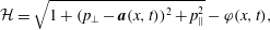 $$\begin{eqnarray}{\mathcal{H}}=\sqrt{1+(p_{\bot }-\boldsymbol{ a}(x,t))^{2}+p_{\Vert }^{2}}-{\it\varphi}(x,t),\end{eqnarray}$$
where
 $p_{\bot }$
and
$p_{\bot }$
and
 $p_{\Vert }$
are the components of the generalized momentum perpendicular and longitudinal with respect to the direction of the electromagnetic wave propagation,
$p_{\Vert }$
are the components of the generalized momentum perpendicular and longitudinal with respect to the direction of the electromagnetic wave propagation,
 $\boldsymbol{a}$
is the vector potential of the laser pulse and
$\boldsymbol{a}$
is the vector potential of the laser pulse and
 ${\it\varphi}$
is the wake-field scalar potential.
${\it\varphi}$
is the wake-field scalar potential.
Neglecting the influence of dispersion on the propagation of electromagnetic waves, we assume that
 $\boldsymbol{a}$
and
$\boldsymbol{a}$
and
 ${\it\varphi}$
depend only on the variable
${\it\varphi}$
depend only on the variable
 $X=x-{\it\beta}_{w}t$
. The Hamiltonian in (3.3) has a symmetry, which implies that there are integrals of motion
$X=x-{\it\beta}_{w}t$
. The Hamiltonian in (3.3) has a symmetry, which implies that there are integrals of motion
 $$\begin{eqnarray}{\mathcal{H}}-{\it\beta}_{w}p=h_{0},\quad p_{\bot }=p_{\bot ,0}.\end{eqnarray}$$
Here and below we use the notation
 $p$
for the longitudinal component of the electron momentum. It then follows that the electron energy at the coordinate
$p$
for the longitudinal component of the electron momentum. It then follows that the electron energy at the coordinate
 $X$
is
$X$
is
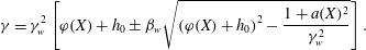 $$\begin{eqnarray}{\it\gamma}={\it\gamma}_{w}^{2}\left[{\it\varphi}(X)+h_{0}\pm {\it\beta}_{w}\sqrt{\left({\it\varphi}(X)+h_{0}\right)^{2}-\frac{1+a(X)^{2}}{{\it\gamma}_{w}^{2}}}\right].\end{eqnarray}$$
Here the plus sign corresponds to the coordinate
 $X$
increasing with time and the minus sign corresponds to decreasing
$X$
increasing with time and the minus sign corresponds to decreasing
 $X$
. The electromagnetic pulse
$X$
. The electromagnetic pulse
 $a(X)$
is given and the electrostatic potential
$a(X)$
is given and the electrostatic potential
 ${\it\varphi}(X)$
is described by the Poisson equation (2.17). The constant
${\it\varphi}(X)$
is described by the Poisson equation (2.17). The constant
 $h_{0}$
is determined by the initial conditions at
$h_{0}$
is determined by the initial conditions at
 $X=X_{0}$
:
$X=X_{0}$
:
 $$\begin{eqnarray}h_{0}=\sqrt{1+a^{2}(X_{0})+p_{0}^{2}}-{\it\beta}_{w}p_{0}-{\it\varphi}(X_{0})\end{eqnarray}$$
with
 $p_{0}$
being the longitudinal component of the electron momentum at
$p_{0}$
being the longitudinal component of the electron momentum at
 $X=X_{0}$
.
$X=X_{0}$
.
If an ultra-relativistic electron is injected into the wake field with an energy
 ${\it\gamma}_{0}$
substantially higher than
${\it\gamma}_{0}$
substantially higher than
 $2\sqrt{1+a^{2}}$
the constant
$2\sqrt{1+a^{2}}$
the constant
 $h_{0}$
given by (3.6) is approximately equal to
$h_{0}$
given by (3.6) is approximately equal to
 ${\it\gamma}_{0}(1-{\it\beta}_{w})-{\it\varphi}_{0}$
, where
${\it\gamma}_{0}(1-{\it\beta}_{w})-{\it\varphi}_{0}$
, where
 ${\it\varphi}_{0}={\it\varphi}(X_{0})$
. In this limit, the relative energy gain is
${\it\varphi}_{0}={\it\varphi}(X_{0})$
. In this limit, the relative energy gain is
 $$\begin{eqnarray}\frac{{\it\gamma}(X)-{\it\gamma}_{0}}{{\it\gamma}_{0}}=\frac{{\it\varphi}(X)-{\it\varphi}_{0}}{{\it\gamma}_{0}(1-{\it\beta}_{w})}.\end{eqnarray}$$
As we see, it is of the order of or less than
 $(2a^{4}+a^{2})/(1+a^{2})^{3/2}$
, which for
$(2a^{4}+a^{2})/(1+a^{2})^{3/2}$
, which for
 $|a|\gg 1$
is about
$|a|\gg 1$
is about
 $|a|$
. Here we have assumed that
$|a|$
. Here we have assumed that
 ${\it\varphi}(X)$
equals the electrostatic potential maximum
${\it\varphi}(X)$
equals the electrostatic potential maximum
 ${\it\varphi}_{max}=a^{2}$
and
${\it\varphi}_{max}=a^{2}$
and
 ${\it\varphi}_{0}$
is equal to the potential minimum
${\it\varphi}_{0}$
is equal to the potential minimum
 ${\it\varphi}_{min}=-a^{2}/(1+a^{2})$
(see (2.25)). To increase the relative energy gain one should consider an as low as possible initial electron energy
${\it\varphi}_{min}=-a^{2}/(1+a^{2})$
(see (2.25)). To increase the relative energy gain one should consider an as low as possible initial electron energy
 ${\it\gamma}_{0}$
provided it is above the injection energy threshold. The injection threshold can be found from the condition of the radical expression on the right-hand side of (3.5) vanishing, i.e.
${\it\gamma}_{0}$
provided it is above the injection energy threshold. The injection threshold can be found from the condition of the radical expression on the right-hand side of (3.5) vanishing, i.e.
 $$\begin{eqnarray}({\it\varphi}(X)+h_{0})^{2}-\frac{1+a(X)^{2}}{{\it\gamma}_{w}^{2}}=0.\end{eqnarray}$$
Taking into account that at the injection point
 ${\it\varphi}(X)={\it\varphi}_{0}$
we obtain from (3.5) for the injection energy threshold:
${\it\varphi}(X)={\it\varphi}_{0}$
we obtain from (3.5) for the injection energy threshold:
 $$\begin{eqnarray}{\it\gamma}_{inj}=\sqrt{1+a^{2}}{\it\gamma}_{w},\end{eqnarray}$$
inside the laser pulse and
 ${\it\gamma}_{inj}={\it\gamma}_{w}$
behind the pulse. The electron velocity at the injection threshold
${\it\gamma}_{inj}={\it\gamma}_{w}$
behind the pulse. The electron velocity at the injection threshold
 ${\it\beta}_{inj}=p_{inj}/{\it\gamma}_{inj}$
with
${\it\beta}_{inj}=p_{inj}/{\it\gamma}_{inj}$
with
 $p_{inj}={\it\beta}_{w}{\it\gamma}_{w}\sqrt{1+a^{2}}$
, according to (3.9), is equal to the wake wave phase velocity
$p_{inj}={\it\beta}_{w}{\it\gamma}_{w}\sqrt{1+a^{2}}$
, according to (3.9), is equal to the wake wave phase velocity
 ${\it\beta}_{inj}={\it\beta}_{w}$
, which is the condition of electron trapping by the wake field.
${\it\beta}_{inj}={\it\beta}_{w}$
, which is the condition of electron trapping by the wake field.
The injection threshold corresponds to the particle to being at the singular point on the separatrix in the phase space
 $(X,p_{\Vert })$
. From (3.4) and (3.6) we can find the dependence of the electron momentum
$(X,p_{\Vert })$
. From (3.4) and (3.6) we can find the dependence of the electron momentum
 $p_{\Vert }$
on the coordinate
$p_{\Vert }$
on the coordinate
 $X$
. It is given by
$X$
. It is given by
 $$\begin{eqnarray}p_{\Vert }={\it\gamma}_{w}^{2}\left[{\it\beta}_{w}({\it\varphi}(X)+h_{0})\pm \sqrt{({\it\varphi}(X)+h_{0})^{2}-\frac{1+a(X)^{2}}{{\it\gamma}_{w}^{2}}}\right].\end{eqnarray}$$
The separatrix is determined by the constant
 $h_{0}$
equal to
$h_{0}$
equal to
 $h_{s}$
, where
$h_{s}$
, where
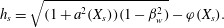 $$\begin{eqnarray}h_{s}=\sqrt{(1+a^{2}(X_{s}))(1-{\it\beta}_{w}^{2})}-{\it\varphi}(X_{s}).\end{eqnarray}$$
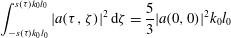
Here
 $X_{s}$
is the coordinate of the singular point, where the potential has a minimum (see figures 1 and 5). The momentum at the singular point equals
$X_{s}$
is the coordinate of the singular point, where the potential has a minimum (see figures 1 and 5). The momentum at the singular point equals
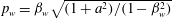 $p_{w}={\it\beta}_{w}\sqrt{(1+a^{2})/(1-{\it\beta}_{w}^{2})}$
. Behind the laser pulse, where
$p_{w}={\it\beta}_{w}\sqrt{(1+a^{2})/(1-{\it\beta}_{w}^{2})}$
. Behind the laser pulse, where
 $a=0$
, the constant
$a=0$
, the constant
 $h_{s}$
is equal to
$h_{s}$
is equal to
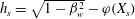 $h_{s}=\sqrt{1-{\it\beta}_{w}^{2}}-{\it\varphi}(X_{s})$
. The electron injected near the singular point
$h_{s}=\sqrt{1-{\it\beta}_{w}^{2}}-{\it\varphi}(X_{s})$
. The electron injected near the singular point
 $X_{s}$
can be accelerated from the momentum
$X_{s}$
can be accelerated from the momentum
 $p_{inj}=p_{w}$
to
$p_{inj}=p_{w}$
to
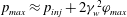 $p_{max}\approx p_{inj}+2{\it\gamma}_{w}^{2}{\it\varphi}_{max}$
, when the trajectory approaches the top of the upper branch of the separatrix, which corresponds to the ‘plus’ sign in (3.10).
$p_{max}\approx p_{inj}+2{\it\gamma}_{w}^{2}{\it\varphi}_{max}$
, when the trajectory approaches the top of the upper branch of the separatrix, which corresponds to the ‘plus’ sign in (3.10).
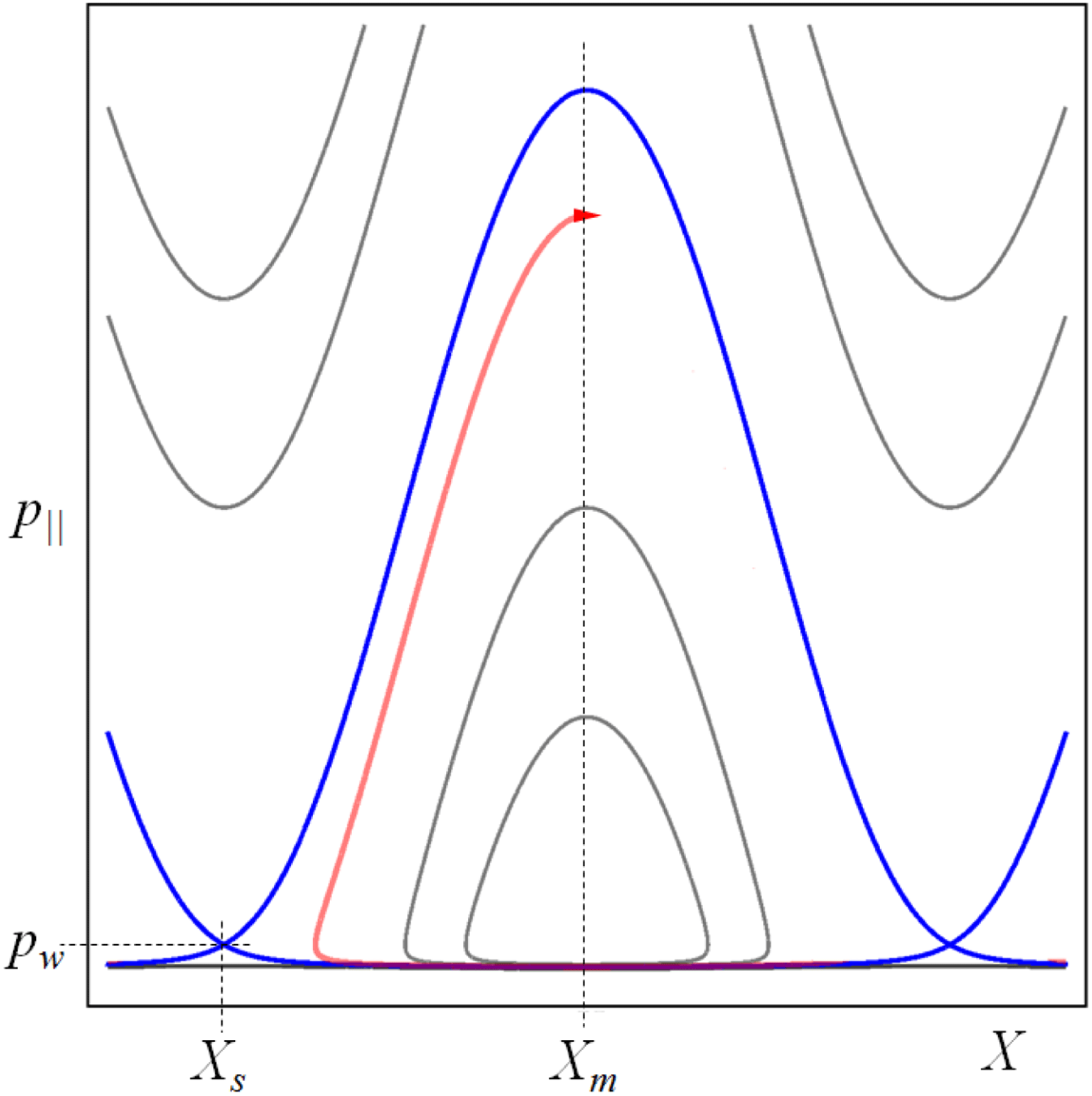
Figure 5. Phase plane
 $(X,p_{\Vert })$
. The singular point at
$(X,p_{\Vert })$
. The singular point at
 $(X_{s},p_{w})$
is a point of crossing of the separatrix branches (blue curves). The particle injected near the bottom of the separatrix within the region enclosed by the separatrix moves along the trajectory (red curve) close to the separatrix.
$(X_{s},p_{w})$
is a point of crossing of the separatrix branches (blue curves). The particle injected near the bottom of the separatrix within the region enclosed by the separatrix moves along the trajectory (red curve) close to the separatrix.
The minimum of the momentum with which the electron can be injected into the accelerating electric field corresponds to the bottom of the separatrix at the point
 $(X_{m},p_{m})$
in the phase plane. At the lower separatrix branch we should take the ‘minus’ sign in (3.10). In the limit
$(X_{m},p_{m})$
in the phase plane. At the lower separatrix branch we should take the ‘minus’ sign in (3.10). In the limit
 ${\it\gamma}_{w}\gg 1$
, the minimum of the momentum is
${\it\gamma}_{w}\gg 1$
, the minimum of the momentum is
 $$\begin{eqnarray}p_{m}\approx {\it\varphi}(X_{m})/2.\end{eqnarray}$$
The electron injected near the bottom of the separatrix within the region enclosed by the separatrices moves along the trajectory close to the separatrix, as shown by the red curve in figure 5. It can reach the momentum
 $p_{max}\approx 2{\it\gamma}_{w}^{2}{\it\varphi}_{max}$
in the vicinity of the top of the separatrix. We note that the electron acceleration time (and the acceleration distance), in this case, is twice as large as the acceleration time for the particle injected at the singular point
$p_{max}\approx 2{\it\gamma}_{w}^{2}{\it\varphi}_{max}$
in the vicinity of the top of the separatrix. We note that the electron acceleration time (and the acceleration distance), in this case, is twice as large as the acceleration time for the particle injected at the singular point
 $X_{s}$
.
$X_{s}$
.
3.2 Effect of plasma inhomogeneity
Plasma inhomogeneity effects can lower the phase velocity of the wake wave left behind the driver laser pulse, thus lowering the injection energy threshold (Bulanov et al. Reference Bulanov, Naumova, Pegoraro and Sakai1998; Fubiani et al. Reference Fubiani, Esarey, Schroeder and Leemans2006; Brantov et al. Reference Brantov, Kando, Kotaki, Yu and Bulanov2008). Within the framework of the approximation assuming that the wake wave is below the wave breaking threshold and assuming, in particular, that the electron displacement inside the wake is substantially less than the scale length of the plasma density inhomogeneity, we can write the phase of the wake wave in the form
 $$\begin{eqnarray}\displaystyle {\it\Psi}(x,t) & = & \displaystyle {\it\omega}_{pe}(x)\left(\int _{0}^{x}\frac{\text{d}x}{v_{g}(x)}-t\right)\nonumber\\ \displaystyle & = & \displaystyle {\it\omega}_{pe}(x)\int _{x_{las}(t)}^{x}\frac{\text{d}x}{v_{g}(x)}.\end{eqnarray}$$
Here
 ${\it\omega}_{pe}(x)$
and
${\it\omega}_{pe}(x)$
and
 $v_{g}(x)$
are the local values of the Langmuir frequency and the laser pulse group velocity (equal to
$v_{g}(x)$
are the local values of the Langmuir frequency and the laser pulse group velocity (equal to
 $v_{g}=k_{0}c^{2}/\sqrt{k_{0}^{2}c^{2}+{\it\omega}_{pe}^{2}(x)}$
), respectively. The function
$v_{g}=k_{0}c^{2}/\sqrt{k_{0}^{2}c^{2}+{\it\omega}_{pe}^{2}(x)}$
), respectively. The function
 $x_{las}(t)$
is the laser pulse coordinate at time
$x_{las}(t)$
is the laser pulse coordinate at time
 $t$
given by the equation
$t$
given by the equation
 $$\begin{eqnarray}\int _{0}^{x_{las}(t)}\frac{\text{d}x}{v_{g}(x)}=t.\end{eqnarray}$$
In a homogeneous plasma the phase (3.13) depends on the variable
 $X$
as
$X$
as
 $$\begin{eqnarray}{\it\Psi}(x,t)=-\frac{{\it\omega}_{pe}X}{v_{g}}.\end{eqnarray}$$
The local wavenumber of the wake wave is the gradient of the phase function,
 $k_{w}=\partial _{x}{\it\Psi}$
, and the local frequency is proportional to its rate of change,
$k_{w}=\partial _{x}{\it\Psi}$
, and the local frequency is proportional to its rate of change,
 ${\it\omega}_{w}=-\partial _{t}{\it\Psi}$
. Differentiating the phase
${\it\omega}_{w}=-\partial _{t}{\it\Psi}$
. Differentiating the phase
 ${\it\Psi}$
, given by (3.13), with respect to time and coordinate we find the frequency and wavenumber of the wake wave as:
${\it\Psi}$
, given by (3.13), with respect to time and coordinate we find the frequency and wavenumber of the wake wave as:
 $$\begin{eqnarray}{\it\omega}_{w}={\it\omega}_{pe}(x),\end{eqnarray}$$
and
 $$\begin{eqnarray}k_{w}=\frac{{\it\omega}_{pe}}{\displaystyle v_{g}(x)-\partial _{x}{\it\omega}_{pe}(x)\int _{x}^{x_{las}(t)}\frac{\text{d}x}{v_{g}(x)}},\end{eqnarray}$$
respectively.
In a downramp density plasma, where the coordinate derivative of the Langmuir frequency is negative, the wavenumber
 $k_{w}(x)$
increases with the growth of the distance between the laser pulse and the point with coordinate
$k_{w}(x)$
increases with the growth of the distance between the laser pulse and the point with coordinate
 $x$
. This corresponds to decreasing of the wake wave phase velocity, defined as
$x$
. This corresponds to decreasing of the wake wave phase velocity, defined as
 $$\begin{eqnarray}v_{w}=\frac{{\it\omega}_{w}}{k_{w}}=v_{g}\frac{{\it\omega}_{pe}}{\displaystyle {\it\omega}_{pe}-v_{g}\partial _{x}{\it\omega}_{pe}\int _{x}^{x_{las}(t)}\frac{\text{d}x}{v_{g}(x)}},\end{eqnarray}$$
i.e. lowering the injection threshold. Eventually the wake wave breaks, as discussed in detail by Bulanov et al. (Reference Bulanov, Naumova, Pegoraro and Sakai1998), Brantov et al. (Reference Brantov, Kando, Kotaki, Yu and Bulanov2008), Lobet et al. (Reference Lobet, Kando, Koga, Esirkepov, Nakamura, Pirozhkov and Bulanov2013). The change of the wake wave wavelength,
 ${\it\lambda}_{w}=2{\rm\pi}/k_{w}$
, leads to a change of the wake wave crest position where the electron injection occurs. The position of the wake wave crest is marked by the value of the phase
${\it\lambda}_{w}=2{\rm\pi}/k_{w}$
, leads to a change of the wake wave crest position where the electron injection occurs. The position of the wake wave crest is marked by the value of the phase
 ${\it\Psi}$
. Using (3.13) we obtain the velocity of the point of constant phase,
${\it\Psi}$
. Using (3.13) we obtain the velocity of the point of constant phase,
 $$\begin{eqnarray}{\dot{x}}_{{\it\Psi}}=v_{g}\frac{{\it\omega}_{pe}^{2}}{{\it\omega}_{pe}^{2}+{\it\Psi}v_{g}\partial _{x}{\it\omega}_{pe}}.\end{eqnarray}$$
The corresponding gamma factor
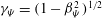 ${\it\gamma}_{{\it\Psi}}=(1-{\it\beta}_{{\it\Psi}}^{2})^{1/2}$
, with
${\it\gamma}_{{\it\Psi}}=(1-{\it\beta}_{{\it\Psi}}^{2})^{1/2}$
, with
 ${\it\beta}_{{\it\Psi}}={\dot{x}}_{{\it\Psi}}/c$
can be written in the limit of low density plasma,
${\it\beta}_{{\it\Psi}}={\dot{x}}_{{\it\Psi}}/c$
can be written in the limit of low density plasma,
 $n/n_{cr}\ll 1$
, as
$n/n_{cr}\ll 1$
, as
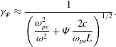 $$\begin{eqnarray}{\it\gamma}_{{\it\Psi}}\approx \frac{1}{\left({\displaystyle \frac{{\it\omega}_{pe}^{2}}{{\it\omega}^{2}}}+{\it\Psi}{\displaystyle \frac{2c}{{\it\omega}_{pe}L}}\right)^{1/2}}.\end{eqnarray}$$
Here we make use of the fact that the laser pulse group velocity is given by
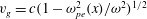 $v_{g}=c(1-{\it\omega}_{pe}^{2}(x)/{\it\omega}^{2})^{1/2}$
and introduce the plasma inhomogeneity scale length
$v_{g}=c(1-{\it\omega}_{pe}^{2}(x)/{\it\omega}^{2})^{1/2}$
and introduce the plasma inhomogeneity scale length
 $L=|{\it\omega}_{pe}/\partial _{x}{\it\omega}_{pe}|$
.
$L=|{\it\omega}_{pe}/\partial _{x}{\it\omega}_{pe}|$
.
As we see, the plasma inhomogeneity effects are important provided the the plasma inhomogeneity scale length is small enough and/or the wake wave phase is sufficiently large:
 $L<2{\it\Psi}c{\it\omega}^{2}/{\it\omega}_{pe}^{3}$
.
$L<2{\it\Psi}c{\it\omega}^{2}/{\it\omega}_{pe}^{3}$
.
Figure 6 illustrates the above discussed effects. Plots are drawn in arbitrary units. Figure 6(a) shows the electron density profile approximated by the expression
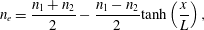 $$\begin{eqnarray}n_{e}=\frac{n_{1}+n_{2}}{2}-\frac{n_{1}-n_{2}}{2}\text{tanh}\left(\frac{x}{L}\right),\end{eqnarray}$$
where
 $n_{1}$
and
$n_{1}$
and
 $n_{2}$
are the electron density at
$n_{2}$
are the electron density at
 $x\rightarrow \pm \infty$
. In the plot (a)
$x\rightarrow \pm \infty$
. In the plot (a)
 $n_{1}=1.5$
,
$n_{1}=1.5$
,
 $n_{2}=1$
and
$n_{2}=1$
and
 $L=5$
. Figure 6(b) presents the trajectories of the constant phase points in the
$L=5$
. Figure 6(b) presents the trajectories of the constant phase points in the
 $(x,t)$
plane. As we see, the distance between the trajectories in the region of the plasma inhomogeneity becomes smaller the larger the time
$(x,t)$
plane. As we see, the distance between the trajectories in the region of the plasma inhomogeneity becomes smaller the larger the time
 $t$
is. In figure 6(c) we see the phase dependence on the coordinate
$t$
is. In figure 6(c) we see the phase dependence on the coordinate
 $x$
at
$x$
at
 $t=t_{m}$
for
$t=t_{m}$
for
 $t_{m}=125$
with decreasing scale of the inhomogeneity in the region in the vicinity of the coordinate
$t_{m}=125$
with decreasing scale of the inhomogeneity in the region in the vicinity of the coordinate
 $x=0$
. Figure 6(d) presents the profile of the wake wave phase velocity
$x=0$
. Figure 6(d) presents the profile of the wake wave phase velocity
 $v_{ph}$
at
$v_{ph}$
at
 $t=0$
,
$t=0$
,
 $0.125t_{m}$
,
$0.125t_{m}$
,
 $0.25t_{m}$
,
$0.25t_{m}$
,
 $0.5t_{m}$
,
$0.5t_{m}$
,
 $0.75t_{m}$
,
$0.75t_{m}$
,
 $t_{m}$
. Within the region of the plasma inhomogeneity, the wake wave phase velocity at first for
$t_{m}$
. Within the region of the plasma inhomogeneity, the wake wave phase velocity at first for
 $x<0$
gradually decreases and then, where
$x<0$
gradually decreases and then, where
 $x>0$
, gradually increases. Within the interval where the phase velocity becomes lower than the electron quiver velocity the wake wave breaks, resulting in electron trapping. Then, the electrons moving together with the wave appear in the region of high phase velocity. During the injection process, the electrons remain trapped by the wave which can be explained by the process similar to the ‘phase stability principle’ of Veksler (Reference Veksler1944), McMillan (Reference McMillan1945).
$x>0$
, gradually increases. Within the interval where the phase velocity becomes lower than the electron quiver velocity the wake wave breaks, resulting in electron trapping. Then, the electrons moving together with the wave appear in the region of high phase velocity. During the injection process, the electrons remain trapped by the wave which can be explained by the process similar to the ‘phase stability principle’ of Veksler (Reference Veksler1944), McMillan (Reference McMillan1945).

Figure 6. Plasma inhomogeneity effects on the phase velocity of the wake wave. (a) Electron density profile given by (3.21) with
 $n_{1}=1.5$
,
$n_{1}=1.5$
,
 $n_{2}=1$
, and
$n_{2}=1$
, and
 $L=5$
. (b) The trajectories of the constant phase points in the
$L=5$
. (b) The trajectories of the constant phase points in the
 $(x,t)$
plane. (c) The phase dependence on the coordinate
$(x,t)$
plane. (c) The phase dependence on the coordinate
 $x$
at
$x$
at
 $t=t_{m}$
for
$t=t_{m}$
for
 $t_{m}=125$
. (d) The wake wave phase velocity
$t_{m}=125$
. (d) The wake wave phase velocity
 $v_{ph}$
versus coordinate
$v_{ph}$
versus coordinate
 $x$
at
$x$
at
 $t=0$
,
$t=0$
,
 $0.125t_{m}$
,
$0.125t_{m}$
,
 $0.25t_{m}$
,
$0.25t_{m}$
,
 $0.5t_{m}$
,
$0.5t_{m}$
,
 $0.75t_{m}$
,
$0.75t_{m}$
,
 $t_{m}$
. Plots are drawn in arbitrary units.
$t_{m}$
. Plots are drawn in arbitrary units.
3.3 Electron injection at the interface between two regions with different plasma density
When the plasma density changes abruptly at the interface between two plasmas the injection mechanism is different from the one considered above. We consider the plasma configuration shown in figure 7 with the plasma density changing from
 $n_{1}$
at
$n_{1}$
at
 $x\rightarrow -\infty$
to
$x\rightarrow -\infty$
to
 $n_{2}$
for
$n_{2}$
for
 $x\rightarrow +\infty$
. At the border between these two plasmas, the electrons with momentum equal to
$x\rightarrow +\infty$
. At the border between these two plasmas, the electrons with momentum equal to
 $p_{1}$
appear inside the wake wave generated by the laser pulse in the lower plasma density region. The momentum
$p_{1}$
appear inside the wake wave generated by the laser pulse in the lower plasma density region. The momentum
 $p_{1}$
equals either
$p_{1}$
equals either
 ${\it\gamma}_{w,1}=({\it\omega}_{0}/{\it\omega}_{pe,1})$
if they are preinjected into the wake field or is approximately equal to the quiver momentum determined by the wake wave amplitude if no preinjection occurs, as in the case of the injection mechanism formulated by Suk et al. (Reference Suk, Barov, Rosenzweig and Esarey2001).
${\it\gamma}_{w,1}=({\it\omega}_{0}/{\it\omega}_{pe,1})$
if they are preinjected into the wake field or is approximately equal to the quiver momentum determined by the wake wave amplitude if no preinjection occurs, as in the case of the injection mechanism formulated by Suk et al. (Reference Suk, Barov, Rosenzweig and Esarey2001).
For the sake of brevity, we assume that the electrons are preinjected, the laser pulse driver of optimal length has amplitude equal to unity and the length of the left-hand side of the plasma region is of the order of the acceleration length. This scenario can be considered as the ‘rephasing’ mechanism of electron energy boost, which has been analysed by Döpp et al. (Reference Döpp, Guillaume, Thaury, Lifschitz, Phuoc and Malka2015), Guillaume et al. (Reference Guillaume, Döpp, Thaury, Ta Phuoc, Lifschitz, Grittani, Goddet, Tafzi, Chou and Veisz2015b ).
In the case under consideration, the electrons with maximum momentum are localized at the top of the separatrix in the phase plane
 $(x,p)$
, as shown in figure 7. The distance between the electron bunch and the front side of the wake wave
$(x,p)$
, as shown in figure 7. The distance between the electron bunch and the front side of the wake wave
 ${\it\delta}x$
is of the order of the laser pulse driver of optimal length given by (2.21). Since both the relativistic electron bunch and the laser pulse move with velocity close to the speed of light, at the time, when they enter the plasma region on right-hand side, the distance between them remains almost unchanged. As a result the electron bunch in the plasma region on left-hand side appears to be relatively close to the front of the wake wave bucket. In order to be further accelerated, the electron bunch should be inside the region in the phase plane enclosed by the separatrix. This is equivalent to the requirements
${\it\delta}x$
is of the order of the laser pulse driver of optimal length given by (2.21). Since both the relativistic electron bunch and the laser pulse move with velocity close to the speed of light, at the time, when they enter the plasma region on right-hand side, the distance between them remains almost unchanged. As a result the electron bunch in the plasma region on left-hand side appears to be relatively close to the front of the wake wave bucket. In order to be further accelerated, the electron bunch should be inside the region in the phase plane enclosed by the separatrix. This is equivalent to the requirements
 $n_{2}/n_{1}\ll 1$
and
$n_{2}/n_{1}\ll 1$
and
 $p_{1}\approx p_{w,2}$
, where the injection momentum
$p_{1}\approx p_{w,2}$
, where the injection momentum
 $p_{inj}=p_{w,2}$
corresponds to the electrons with the energy equal to
$p_{inj}=p_{w,2}$
corresponds to the electrons with the energy equal to
 ${\it\gamma}_{w,2}$
calculated for the phase velocity of the wake wave in the right-hand side region.
${\it\gamma}_{w,2}$
calculated for the phase velocity of the wake wave in the right-hand side region.
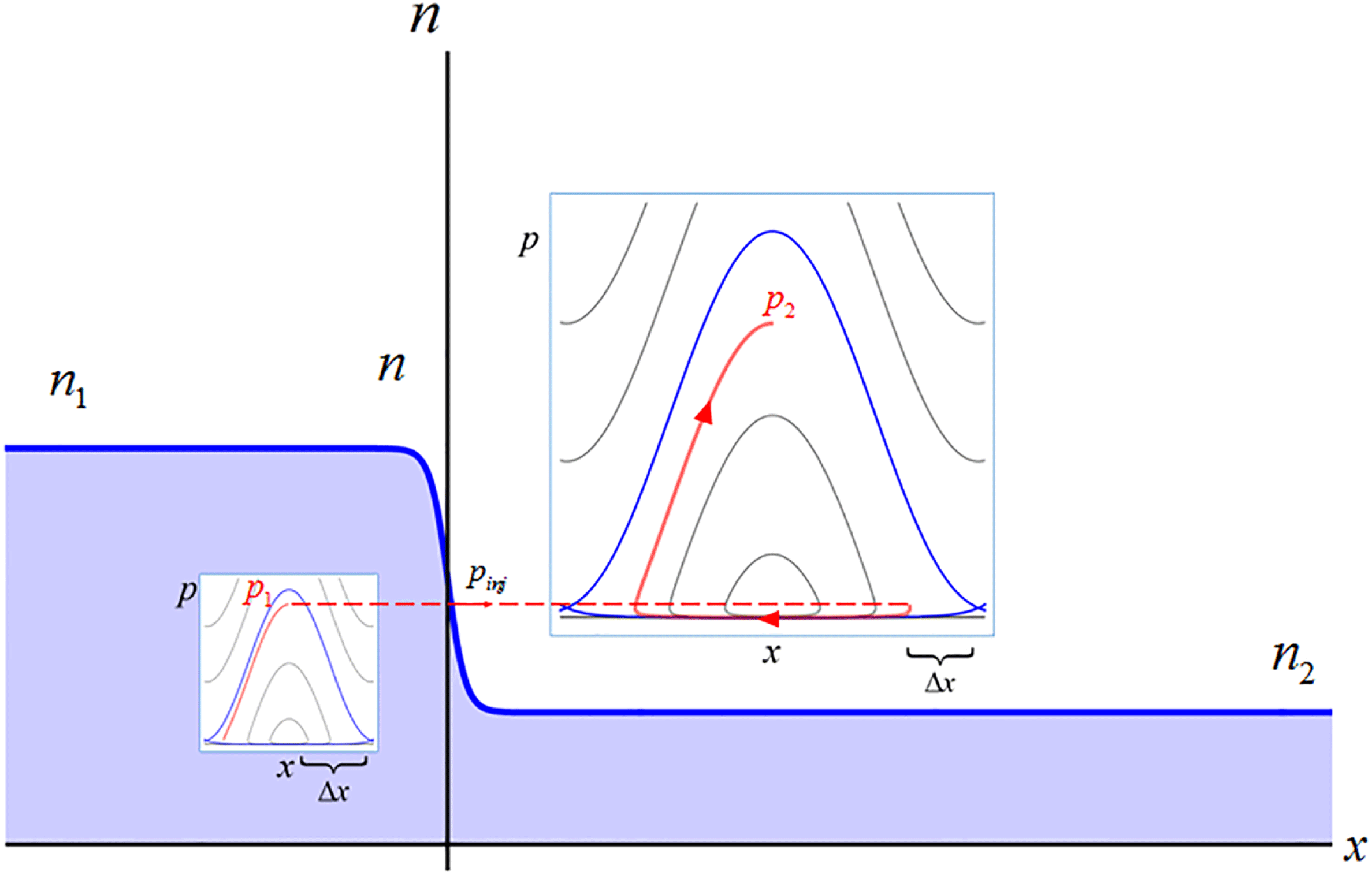
Figure 7. The electron bunch injection/rephasing at the interface between two regions with different plasma density. In the plasma region on the left-hand side with density
 $n_{1}$
the LWFA electron bunch is preaccelerated to momentum
$n_{1}$
the LWFA electron bunch is preaccelerated to momentum
 $p_{1}$
reached at the interface between the two plasmas. In the plasma region on the right-hand side the density is substantially lower than in the region on the left-hand side,
$p_{1}$
reached at the interface between the two plasmas. In the plasma region on the right-hand side the density is substantially lower than in the region on the left-hand side,
 $n_{2}\ll n_{1}$
. Here the electron bunch occurs in the region in the phase plane
$n_{2}\ll n_{1}$
. Here the electron bunch occurs in the region in the phase plane
 $(x,p)$
within the separatrix (provided
$(x,p)$
within the separatrix (provided
 $p_{1}=p_{inj}=p_{w,2}$
) close to the front of the wake wave bucket. Then the electron bunch is accelerated moving along the trajectory (red curve) close to the separatrix.
$p_{1}=p_{inj}=p_{w,2}$
) close to the front of the wake wave bucket. Then the electron bunch is accelerated moving along the trajectory (red curve) close to the separatrix.
If the requirements formulated above are fulfilled, the electron bunch trapped inside the separatrix close the wake wave front then moves along the trajectory in the phase plane shown by the red curve on the upper right-hand side in figure 7. In the limit
 $n_{2}/n_{1}\ll 1$
the energy of accelerated electrons can be of the order of
$n_{2}/n_{1}\ll 1$
the energy of accelerated electrons can be of the order of
 ${\it\gamma}_{w,2}^{2}\approx n_{1}/n_{2}$
.
${\it\gamma}_{w,2}^{2}\approx n_{1}/n_{2}$
.
We note that in the case when the electron bunch appears to be injected at a position too close to the front of the wake wave in the first bucket, the properties of the accelerated electrons such as the transverse emittance, energy spectrum width, etc., can be modified due to interaction with the laser pulse driver (e.g. see Kotaki et al. Reference Kotaki, Kawase, Hayashi, Mori, Kando, Koga and Bulanov2015). In view of this, to optimize the electron injection and/or ‘rephasing’ whilst avoiding the electron–laser interaction the electron bunch should be preaccelerated, or injected, in the second, or third and so on buckets. This can be done by choosing the plasma density inhomogeneity scale length within the framework of the injection mechanism discussed in the previous subsection.

Figure 8. The wake wave left behind the laser pulse of amplitude
 $a=1$
and of the length
$a=1$
and of the length
 $l=27$
propagating in a plasma characterized by
$l=27$
propagating in a plasma characterized by
 ${\it\beta}_{w}=0.9995$
. (a) The electrostatic potential changes inside the pulse between
${\it\beta}_{w}=0.9995$
. (a) The electrostatic potential changes inside the pulse between
 ${\it\varphi}_{max}=1$
and
${\it\varphi}_{max}=1$
and
 ${\it\varphi}_{min}=0$
and between
${\it\varphi}_{min}=0$
and between
 ${\it\varphi}_{max}=1$
and
${\it\varphi}_{max}=1$
and
 ${\it\varphi}_{min}=-1/2$
behind the pulse, respectively. The electric field inside the pulse is smaller than behind. The wake wave wavelength is larger inside the pulse than behind it. (b) The electron density and the laser pulse versus the coordinate
${\it\varphi}_{min}=-1/2$
behind the pulse, respectively. The electric field inside the pulse is smaller than behind. The wake wave wavelength is larger inside the pulse than behind it. (b) The electron density and the laser pulse versus the coordinate
 $X$
.
$X$
.
3.4 Electron acceleration by the wake field
Assuming
 ${\it\varphi}(X)-{\it\varphi}_{0}={\it\varphi}_{max}-{\it\varphi}_{min}$
, which is equal to
${\it\varphi}(X)-{\it\varphi}_{0}={\it\varphi}_{max}-{\it\varphi}_{min}$
, which is equal to
 $(2a^{4}+a^{4})/(1+a^{2})$
in the case of electron injection to the wake wave behind the laser pulse and to
$(2a^{4}+a^{4})/(1+a^{2})$
in the case of electron injection to the wake wave behind the laser pulse and to
 $a^{2}$
when the injection phase corresponds to the wake wave inside the laser pulse, we find the maximal electron energy. In the case of the electron acceleration in the wake field behind the laser pulse, the energy is
$a^{2}$
when the injection phase corresponds to the wake wave inside the laser pulse, we find the maximal electron energy. In the case of the electron acceleration in the wake field behind the laser pulse, the energy is
 $$\begin{eqnarray}{\it\gamma}={\it\gamma}_{inj}+\frac{a^{4}+2a^{2}}{(1-{\it\beta}_{w})(1+a^{2})},\end{eqnarray}$$
and it is equal to
 $$\begin{eqnarray}{\it\gamma}={\it\gamma}_{inj}+\frac{a^{2}}{1-{\it\beta}_{w}},\end{eqnarray}$$
when the acceleration occurs in the wake field inside the laser pulse.
In figure 8 we show the electrostatic potential and electric field in the wake wave generated by a flat top laser pulse of amplitude
 $a=1$
and of length
$a=1$
and of length
 $l=27$
propagating in a plasma characterized by
$l=27$
propagating in a plasma characterized by
 ${\it\beta}_{w}=0.9995$
. For these parameters (3.22) and (3.23) give for the normalized energy of the accelerated electrons with values equal to
${\it\beta}_{w}=0.9995$
. For these parameters (3.22) and (3.23) give for the normalized energy of the accelerated electrons with values equal to
 ${\it\gamma}_{e}=3000$
in the case of electron acceleration in the wake field behind the laser pulse, and to
${\it\gamma}_{e}=3000$
in the case of electron acceleration in the wake field behind the laser pulse, and to
 ${\it\gamma}_{e}=2000$
when the acceleration occurs in the wake field inside the laser pulse, respectively. The electrostatic potential varies in the wake inside the pulse between
${\it\gamma}_{e}=2000$
when the acceleration occurs in the wake field inside the laser pulse, respectively. The electrostatic potential varies in the wake inside the pulse between
 ${\it\varphi}_{max}=1$
and
${\it\varphi}_{max}=1$
and
 ${\it\varphi}_{min}=0$
and it changes between
${\it\varphi}_{min}=0$
and it changes between
 ${\it\varphi}_{max}=1$
and
${\it\varphi}_{max}=1$
and
 ${\it\varphi}_{min}=-1/2$
behind the pulse, respectively. The electric field inside the pulse is smaller than behind.
${\it\varphi}_{min}=-1/2$
behind the pulse, respectively. The electric field inside the pulse is smaller than behind.

Figure 9. The phase plane
 $(X,p)$
for the same laser–plasma parameters as in figure 8. The inset on the right-hand side shows a zoomed
$(X,p)$
for the same laser–plasma parameters as in figure 8. The inset on the right-hand side shows a zoomed
 $(15<X<30)$
part of the phase plane. The inset on the left-hand side shows a zoomed
$(15<X<30)$
part of the phase plane. The inset on the left-hand side shows a zoomed
 $(-25<X<-5)$
part of the phase plane.
$(-25<X<-5)$
part of the phase plane.
The wake wave wavelength is larger inside the pulse than behind it. Figure 8(b) shows the electron density and the laser pulse versus the coordinate
 $X$
. As we see, the electron density modulations are stronger in the wake wave behind the laser pulse than inside it. This may have important implications in the Relativistic Flying Mirror paradigm (see review articles Bulanov et al. (Reference Bulanov, Esirkepov, Kando, Pirozhkov and Rosanov2013a
), Bulanov et al. (Reference Bulanov, Esirkepov, Kando and Koga2016) and literature cited therein), because the larger the electron density modulations in the wake wave the higher the reflectivity of the dense electron layer is.
$X$
. As we see, the electron density modulations are stronger in the wake wave behind the laser pulse than inside it. This may have important implications in the Relativistic Flying Mirror paradigm (see review articles Bulanov et al. (Reference Bulanov, Esirkepov, Kando, Pirozhkov and Rosanov2013a
), Bulanov et al. (Reference Bulanov, Esirkepov, Kando and Koga2016) and literature cited therein), because the larger the electron density modulations in the wake wave the higher the reflectivity of the dense electron layer is.
Figure 9 presents the electron phase plane
 $(X,p)$
for the same laser–plasma parameters as in figure 8. The injection energy given by (3.9) is equal to 31.6 behind the laser pulse and to 44.7 inside the laser pulse, respectively.
$(X,p)$
for the same laser–plasma parameters as in figure 8. The injection energy given by (3.9) is equal to 31.6 behind the laser pulse and to 44.7 inside the laser pulse, respectively.
In the case of an ultra-short laser pulse, by using (2.31) we can obtain for the accelerated electron energy
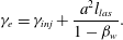 $$\begin{eqnarray}{\it\gamma}_{e}={\it\gamma}_{inj}+\frac{a^{2}l_{las}}{1-{\it\beta}_{w}}.\end{eqnarray}$$
We have assumed that
 $a^{2}l_{las}\ll 1$
. As we have seen above and as noted by Esirkepov et al. (Reference Esirkepov, Bulanov, Yamagiwa and Tajima2006) the laser-driven wake field is not periodical, and a thorough analysis of the electron dynamics in the vicinity of the laser pulse front is of great importance. In Khachatryan et al. (Reference Khachatryan, van Goor, Boller, Reitsma and Jaroszynski2004), the localized electron energy spectrum was attributed to electrons with velocity greater than the velocity of the laser pulse front
$a^{2}l_{las}\ll 1$
. As we have seen above and as noted by Esirkepov et al. (Reference Esirkepov, Bulanov, Yamagiwa and Tajima2006) the laser-driven wake field is not periodical, and a thorough analysis of the electron dynamics in the vicinity of the laser pulse front is of great importance. In Khachatryan et al. (Reference Khachatryan, van Goor, Boller, Reitsma and Jaroszynski2004), the localized electron energy spectrum was attributed to electrons with velocity greater than the velocity of the laser pulse front
 ${\it\beta}_{w}$
that overtake the laser pulse due to acceleration in the wake-field first cycle. At the laser pulse front, conditions can be met for the so-called ‘ponderomotive’ electron acceleration. In figure 9 these trajectories correspond to the horizontal lines ahead of the laser pulse. It is easy to see that the energy gain is equal to zero if the electrons have been injected to the acceleration phase of the wake field inside the laser pulse. In this case, when the electrons are injected into the region behind the pulse then when they have overtaken the pulse their energy becomes equal to
${\it\beta}_{w}$
that overtake the laser pulse due to acceleration in the wake-field first cycle. At the laser pulse front, conditions can be met for the so-called ‘ponderomotive’ electron acceleration. In figure 9 these trajectories correspond to the horizontal lines ahead of the laser pulse. It is easy to see that the energy gain is equal to zero if the electrons have been injected to the acceleration phase of the wake field inside the laser pulse. In this case, when the electrons are injected into the region behind the pulse then when they have overtaken the pulse their energy becomes equal to
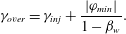 $$\begin{eqnarray}{\it\gamma}_{over}={\it\gamma}_{inj}+\frac{|{\it\varphi}_{min}|}{1-{\it\beta}_{w}}.\end{eqnarray}$$
If the laser pulse has the length optimal for wake-field generation (see (2.21)), the energy gain is
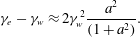 $$\begin{eqnarray}{\it\gamma}_{e}-{\it\gamma}_{w}\approx 2{\it\gamma}_{w}^{2}\frac{a^{2}}{(1+a^{2})}.\end{eqnarray}$$
Which scales as the square of the wake wave gamma factor,
 $\propto {\it\gamma}_{w}^{2}$
.
$\propto {\it\gamma}_{w}^{2}$
.
3.5 Energy spectrum
When a relatively long, initially quasi-monoenergetic, electron bunch is injected at the minimum of the electrostatic potential and accelerated by the wake-field wave, its particles are distributed along the separatrix with some density
 ${\mathcal{N}}(X)$
. This results in the particle energy spectrum broadening from the initial energy
${\mathcal{N}}(X)$
. This results in the particle energy spectrum broadening from the initial energy
 ${\it\gamma}_{inj}\approx {\it\gamma}_{w}$
to the maximum energy
${\it\gamma}_{inj}\approx {\it\gamma}_{w}$
to the maximum energy
 ${\it\gamma}_{max}$
. Besides these two limits, the spectrum has peculiarities as noticed by Bulanov & Tajima (Reference Bulanov and Tajima2005), Bulanov et al. (Reference Bulanov, Yamagiwa, Esirkepov, Koga, Kando, Ueshima, Saito and Wakabayashi2005), Esirkepov et al. (Reference Esirkepov, Bulanov, Yamagiwa and Tajima2006). Near the top of the separatrix, the particle energy has a parabolic dependence on
${\it\gamma}_{max}$
. Besides these two limits, the spectrum has peculiarities as noticed by Bulanov & Tajima (Reference Bulanov and Tajima2005), Bulanov et al. (Reference Bulanov, Yamagiwa, Esirkepov, Koga, Kando, Ueshima, Saito and Wakabayashi2005), Esirkepov et al. (Reference Esirkepov, Bulanov, Yamagiwa and Tajima2006). Near the top of the separatrix, the particle energy has a parabolic dependence on
 $X$
$X$
 $$\begin{eqnarray}{\it\gamma}_{e}(X)\approx {\it\gamma}_{max}\left[1-\frac{(X_{t}-X)^{2}}{l_{acc}^{2}}\right],\end{eqnarray}$$
with the acceleration length determined by (3.2). This is a consequence of the local parabolic profile of the electrostatic potential in the wake wave near its maximum. The energy spectrum of particles collected over the wake-field period, i.e. integrated over the coordinate
 $X$
, in the vicinity of the maximum energy is determined by the contribution from particles with energy near the maximum:
$X$
, in the vicinity of the maximum energy is determined by the contribution from particles with energy near the maximum:
 $$\begin{eqnarray}\left.\frac{\text{d}N}{\text{d}{\it\gamma}_{e}}\right|_{{\it\gamma}_{e}\rightarrow {\it\gamma}_{max}-0}=\frac{{\mathcal{N}}(X)}{|\text{d}{\it\gamma}_{e}/\text{d}X|}\approx \frac{{\mathcal{N}}(X_{t})l_{acc}}{2\sqrt{{\it\gamma}_{max}\left({\it\gamma}_{max}-{\it\gamma}_{e}\right)}},\end{eqnarray}$$
where
 ${\it\gamma}<{\it\gamma}_{max}$
. The spectrum has an integrable singularity at
${\it\gamma}<{\it\gamma}_{max}$
. The spectrum has an integrable singularity at
 ${\it\gamma}\rightarrow {\it\gamma}_{max}$
. In addition, it has a rather large spread; e.g. half of the particles occupy the energy interval
${\it\gamma}\rightarrow {\it\gamma}_{max}$
. In addition, it has a rather large spread; e.g. half of the particles occupy the energy interval
 $3{\it\gamma}_{max}/4{\it\gamma}<{\it\gamma}_{max}$
. Due to these properties the spectrum has been called ‘quasi-monoenergetic’ (Bulanov & Tajima Reference Bulanov and Tajima2005; Bulanov et al.
Reference Bulanov, Yamagiwa, Esirkepov, Koga, Kando, Ueshima, Saito and Wakabayashi2005).
$3{\it\gamma}_{max}/4{\it\gamma}<{\it\gamma}_{max}$
. Due to these properties the spectrum has been called ‘quasi-monoenergetic’ (Bulanov & Tajima Reference Bulanov and Tajima2005; Bulanov et al.
Reference Bulanov, Yamagiwa, Esirkepov, Koga, Kando, Ueshima, Saito and Wakabayashi2005).
A contribution to the spectrum from particles overtaking the laser pulse can be obtained from the dependence given by (3.25). Taking, for simplicity, the model dependence
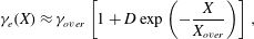 $$\begin{eqnarray}{\it\gamma}_{e}(X)\approx {\it\gamma}_{over}\left[1+D\exp \left(-\frac{X}{X_{over}}\right)\right],\end{eqnarray}$$
where the constant
 $D\approx {\it\gamma}_{max}/{\it\gamma}_{over}$
and
$D\approx {\it\gamma}_{max}/{\it\gamma}_{over}$
and
 $X_{over}$
is a coordinate of a point ahead of the laser pulse, we obtain
$X_{over}$
is a coordinate of a point ahead of the laser pulse, we obtain
 $$\begin{eqnarray}\left.\frac{\text{d}N}{\text{d}{\it\gamma}_{e}}\right|_{{\it\gamma}_{e}\rightarrow {\it\gamma}_{over}+0}=\frac{{\mathcal{N}}(X)}{|\text{d}{\it\gamma}_{e}/\text{d}X|}\approx \frac{{\mathcal{N}}(X_{over})X_{over}}{{\it\gamma}_{e}-{\it\gamma}_{over}}.\end{eqnarray}$$
3.6 Inverse problem of LFWA
As we see from (3.27) and from expressions obtained above for the electrostatic potential in the wake wave, the energy spectrum of the accelerated electrons is determined by the potential profile near its maximum. The spectrum is narrower for flatter potential profiles. In order to find the conditions for wake wave generation with such a dependence of the potential on the spatial coordinate, we analyse (2.8) considering it as an equation for the laser pulse profile required for generating a wake field with the desired parameters. This gives for the laser pulse profile the expression
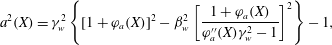 $$\begin{eqnarray}a^{2}(X)={\it\gamma}_{w}^{2}\left\{[1+{\it\varphi}_{a}(X)]^{2}-{\it\beta}_{w}^{2}\left[\frac{1+{\it\varphi}_{a}(X)}{{\it\varphi}_{a}^{\prime \prime }(X){\it\gamma}_{w}^{2}-1}\right]^{2}\right\}-1,\end{eqnarray}$$
with given dependence
 ${\it\varphi}_{a}(X)$
.
${\it\varphi}_{a}(X)$
.
Actually, the realization of a wake field with the desired parameters by using the driver laser pulse given by (3.31) requires the boundary conditions to be fulfilled with high enough precision. In order to reveal the discrepancy (it is also called the ‘residual’) we, as a typical example, assume the super-Gaussian profile for the electrostatic potential:
 $$\begin{eqnarray}{\it\varphi}_{a}(X)=F\exp \left[-\left(\frac{X}{L}\right)^{2q}\right]\end{eqnarray}$$
with the index
 $q>1$
and width
$q>1$
and width
 $L$
. Substituting
$L$
. Substituting
 $a^{2}(X)$
obtained from (3.31) and (3.32) into the right-hand side of (2.8) we solve it numerically for the boundary conditions
$a^{2}(X)$
obtained from (3.31) and (3.32) into the right-hand side of (2.8) we solve it numerically for the boundary conditions
 ${\it\varphi}=0$
and
${\it\varphi}=0$
and
 ${\it\varphi}^{\prime }=0$
at a coordinate far enough ahead the driver pulse. The results are presented in figures 10 and 11.
${\it\varphi}^{\prime }=0$
at a coordinate far enough ahead the driver pulse. The results are presented in figures 10 and 11.
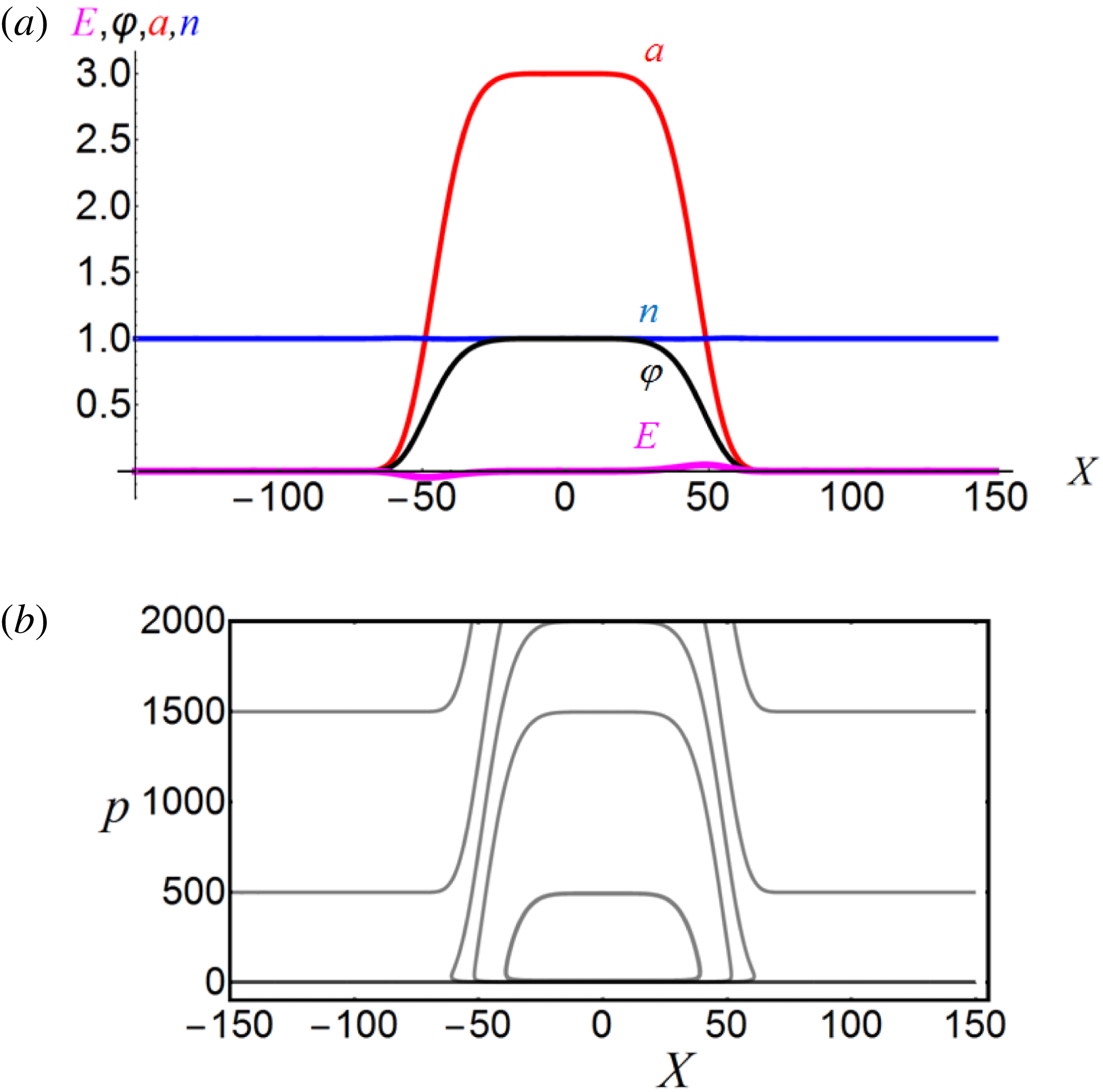
Figure 10. (a) Electrostatic potential, electric field, electron density and the laser pulse (dashed line) versus the coordinate
 $X$
. (b) The electron phase plane
$X$
. (b) The electron phase plane
 $(X,p)$
. The laser pulse corresponding to the trial potential
$(X,p)$
. The laser pulse corresponding to the trial potential
 ${\it\varphi}_{a}$
given by (3.32) having index
${\it\varphi}_{a}$
given by (3.32) having index
 $2q=6$
, length
$2q=6$
, length
 $L=50$
and amplitude
$L=50$
and amplitude
 $F=1$
propagating in a plasma characterized by
$F=1$
propagating in a plasma characterized by
 ${\it\beta}_{w}=0.9995$
(
${\it\beta}_{w}=0.9995$
(
 ${\it\gamma}_{w}=31.6$
).
${\it\gamma}_{w}=31.6$
).
In figure 10 we present the case of a relatively long laser pulse corresponding to the trial potential
 ${\it\varphi}_{a}$
given by (3.32) having index
${\it\varphi}_{a}$
given by (3.32) having index
 $2q=6$
, length
$2q=6$
, length
 $L=50$
and amplitude
$L=50$
and amplitude
 $F=1$
propagating in a plasma characterized by
$F=1$
propagating in a plasma characterized by
 ${\it\beta}_{w}=0.9995$
(
${\it\beta}_{w}=0.9995$
(
 ${\it\gamma}_{w}=31.6$
). The laser pulse generates the electrostatic potential and electric field shown in figure 10(a). The electrostatic potential and electric field are well localized within the region where the laser pulse is. The electron density perturbations are weak, as seen in figure 10. The electron trajectories in the phase plane
${\it\gamma}_{w}=31.6$
). The laser pulse generates the electrostatic potential and electric field shown in figure 10(a). The electrostatic potential and electric field are well localized within the region where the laser pulse is. The electron density perturbations are weak, as seen in figure 10. The electron trajectories in the phase plane
 $(X,p)$
, plotted in figure 10(b), demonstrate that the normalized momentum for the electron trajectory on the separatrix equals 1000. In this case, the laser–plasma interaction can be described within the framework of the adiabatic approximation assuming that the left-hand side of (2.8) vanishes. This yields for the electrostatic potential
$(X,p)$
, plotted in figure 10(b), demonstrate that the normalized momentum for the electron trajectory on the separatrix equals 1000. In this case, the laser–plasma interaction can be described within the framework of the adiabatic approximation assuming that the left-hand side of (2.8) vanishes. This yields for the electrostatic potential
 $$\begin{eqnarray}{\it\varphi}(X)=\sqrt{1+a^{2}(X)}-1.\end{eqnarray}$$
Near the top of the separatrix, the particle energy has a dependence on
 $X$
given by the expression
$X$
given by the expression
 $$\begin{eqnarray}{\it\gamma}_{e}(X)\approx {\it\gamma}_{max}\left[1-\frac{(X_{t}-X)^{2q}}{l_{acc}^{2q}}\right].\end{eqnarray}$$
The energy spectrum of particles collected over the wake-field period, in the vicinity of the maximum energy, is determined by the contribution from particles with energy near the maximum:
 $$\begin{eqnarray}\left.\frac{\text{d}N}{\text{d}{\it\gamma}_{e}}\right|_{{\it\gamma}_{e}\rightarrow {\it\gamma}_{max}-0}\approx \frac{{\mathcal{N}}l_{acc}}{2^{1/2q}\left[{\it\gamma}_{max}\left({\it\gamma}_{max}-{\it\gamma}_{e}\right)\right]^{(2q-1)/2q}},\end{eqnarray}$$
where
 ${\it\gamma}_{e}<{\it\gamma}_{max}$
. The spectrum has an integrable singularity at
${\it\gamma}_{e}<{\it\gamma}_{max}$
. The spectrum has an integrable singularity at
 ${\it\gamma}_{e}\rightarrow {\it\gamma}_{max}$
. In addition, it has a rather large spread; e.g. half of the particles occupy the energy interval
${\it\gamma}_{e}\rightarrow {\it\gamma}_{max}$
. In addition, it has a rather large spread; e.g. half of the particles occupy the energy interval
 ${\it\gamma}_{max}(1-2^{-2q})<{\it\gamma}_{e}<{\it\gamma}_{max}$
. This expression can be rewritten in the form
${\it\gamma}_{max}(1-2^{-2q})<{\it\gamma}_{e}<{\it\gamma}_{max}$
. This expression can be rewritten in the form
 $$\begin{eqnarray}\frac{{\rm\Delta}{\it\gamma}_{e}}{{\it\gamma}_{max}}=2^{-2q},\end{eqnarray}$$
where
 ${\rm\Delta}{\it\gamma}_{e}={\it\gamma}_{max}(1-2^{-2q})-{\it\gamma}_{max}$
. As we see, the larger the index
${\rm\Delta}{\it\gamma}_{e}={\it\gamma}_{max}(1-2^{-2q})-{\it\gamma}_{max}$
. As we see, the larger the index
 $2q$
is, the narrower the energy spectrum is.
$2q$
is, the narrower the energy spectrum is.
If the laser pulse is approximately three times shorter than in the case considered above, the discrepancy between the trial potential
 ${\it\varphi}_{a}$
given by (3.32) and the electrostatic potential generated in the plasma becomes significant, as clearly seen in figure 11, where we present the same dependences as in figure 10 for the laser pulse with length equal to
${\it\varphi}_{a}$
given by (3.32) and the electrostatic potential generated in the plasma becomes significant, as clearly seen in figure 11, where we present the same dependences as in figure 10 for the laser pulse with length equal to
 $L=15$
. The wake wave excited at the front and rear side of the laser pulse substantially modulates the electrostatic potential dependence on the coordinate
$L=15$
. The wake wave excited at the front and rear side of the laser pulse substantially modulates the electrostatic potential dependence on the coordinate
 $X$
. This will result in an accelerated electron energy spectrum with multiple maxima, in whose vicinities the spectrum can be approximated by the expression (3.28).
$X$
. This will result in an accelerated electron energy spectrum with multiple maxima, in whose vicinities the spectrum can be approximated by the expression (3.28).


4 Energy scaling
Due to relativistic self-focusing (Litvak Reference Litvak1970; Sun et al.
Reference Sun, Ott, Lee and Guzdar1987) the laser pulse amplitude and waist are different from their values in a vacuum. Taking into account the self-focusing resulting from the laser pulse channelling inside a channel of radius
 $r_{c}=\sqrt{a}$
(in dimensional units it is
$r_{c}=\sqrt{a}$
(in dimensional units it is
 $r_{c}=c\sqrt{a}/{\it\omega}_{pe}$
), we find a relationship between the electromagnetic wave amplitude and power
$r_{c}=c\sqrt{a}/{\it\omega}_{pe}$
), we find a relationship between the electromagnetic wave amplitude and power
 ${\mathcal{P}}$
(e.g. see Gordienko & Pukhov Reference Gordienko and Pukhov2005; Lu et al.
Reference Lu, Tzoufras, Joshi, Tsung, Mori, Vieira, Fonseca and Silva2007; Bulanov et al.
Reference Bulanov, Brantov, Bychenkov, Chvykov, Kalinchenko, Matsuoka, Rousseau, Reed, Yanovsky and Litzenberg2008b
),
${\mathcal{P}}$
(e.g. see Gordienko & Pukhov Reference Gordienko and Pukhov2005; Lu et al.
Reference Lu, Tzoufras, Joshi, Tsung, Mori, Vieira, Fonseca and Silva2007; Bulanov et al.
Reference Bulanov, Brantov, Bychenkov, Chvykov, Kalinchenko, Matsuoka, Rousseau, Reed, Yanovsky and Litzenberg2008b
),
 $$\begin{eqnarray}a^{3}=\frac{{\mathcal{P}}}{\bar{{\mathcal{P}}}}\left(\frac{{\it\omega}_{pe}}{{\it\omega}}\right)^{2},\end{eqnarray}$$
where the power characteristic in the theory of relativistic self-focusing is
 $$\begin{eqnarray}\bar{{\mathcal{P}}}=2m_{e}^{2}c^{5}/e^{2}\approx 1.74\times 10^{16}~\text{erg}~\text{s}^{-1}\approx 17.4~\text{GW}.\end{eqnarray}$$
The criterion for self-focusing is
 $$\begin{eqnarray}{\mathcal{P}}>\bar{{\mathcal{P}}}\left(\frac{{\it\omega}}{{\it\omega}_{pe}}\right)^{2}.\end{eqnarray}$$
A finite waist laser pulse generates a wake field of the form called the ‘cavity’, ‘blowout’ and/or ‘bubble’ (see Pukhov & Meyer-ter Vehn Reference Pukhov and Meyer-ter Vehn2002; Gordienko & Pukhov Reference Gordienko and Pukhov2005; Lu et al.
Reference Lu, Tzoufras, Joshi, Tsung, Mori, Vieira, Fonseca and Silva2007). The transverse size of the cavity is of the order of
 $\sqrt{a}$
. The form of the cavity in the electron density behind the laser pulse can be found from the fact that all electrons in the way of the laser pulse are pushed aside, forming a multi-stream configuration in the collisionless plasma (Esirkepov, Kato & Bulanov Reference Esirkepov, Kato and Bulanov2008). The plasma inside the cavity is positively charged. It attracts those electrons from the side regions that have not experienced the ponderomotive force action.
$\sqrt{a}$
. The form of the cavity in the electron density behind the laser pulse can be found from the fact that all electrons in the way of the laser pulse are pushed aside, forming a multi-stream configuration in the collisionless plasma (Esirkepov, Kato & Bulanov Reference Esirkepov, Kato and Bulanov2008). The plasma inside the cavity is positively charged. It attracts those electrons from the side regions that have not experienced the ponderomotive force action.
The electrostatic potential inside the cavity is approximately
 ${\it\varphi}_{c}=a$
and the electric field is of the order of
${\it\varphi}_{c}=a$
and the electric field is of the order of
 $\sqrt{a}$
. Using these expressions and (4.1) we can find the accelerated electron energy expressed in terms of the laser power and plasma density (via the ratio
$\sqrt{a}$
. Using these expressions and (4.1) we can find the accelerated electron energy expressed in terms of the laser power and plasma density (via the ratio
 ${\it\omega}/{\it\omega}_{pe}$
), we find
${\it\omega}/{\it\omega}_{pe}$
), we find
 $$\begin{eqnarray}{\it\gamma}_{e}\approx \left(\frac{{\mathcal{P}}}{\bar{{\mathcal{P}}}}\frac{{\it\omega}}{{\it\omega}_{pe}}\right)^{2/3},\end{eqnarray}$$
where we have taken into account the dependence of the laser group velocity and the pulse etching velocity on the laser amplitude. As we see, the fast electron energy is for a given laser power higher for lower plasma density, i.e. as high as the ratio
 ${\it\omega}/{\it\omega}_{pe}$
is. However, since the self-focusing condition (4.3) imposes a constraint on the maximum of this ratio, the maximal electron energy scales as
${\it\omega}/{\it\omega}_{pe}$
is. However, since the self-focusing condition (4.3) imposes a constraint on the maximum of this ratio, the maximal electron energy scales as
 $$\begin{eqnarray}{\it\gamma}_{e,m}\approx \left(\frac{{\mathcal{P}}}{\bar{{\mathcal{P}}}}\right).\end{eqnarray}$$
From this expression it follows that to obtain 1 GeV electrons with a 1 PW power laser pulse the plasma density should be equal to
 $4.3\times 10^{18}~\text{cm}^{-3}$
. Under these conditions, the laser pulse amplitude equals
$4.3\times 10^{18}~\text{cm}^{-3}$
. Under these conditions, the laser pulse amplitude equals
 $a=3$
and the acceleration length
$a=3$
and the acceleration length
 $l_{acc}\approx 2~\text{cm}$
.
$l_{acc}\approx 2~\text{cm}$
.
According (4.5) a PW class laser can provide electrons with the energy of the order of 25 GeV. With a 200 TW laser the achievable electron energy is approximately 5 GeV. The acceleration length
 $l_{acc}\approx {\it\lambda}({\mathcal{P}}/\bar{{\mathcal{P}}})^{3/2}$
is equal to 30 m in the first case and is equal to 75 cm in the second.
$l_{acc}\approx {\it\lambda}({\mathcal{P}}/\bar{{\mathcal{P}}})^{3/2}$
is equal to 30 m in the first case and is equal to 75 cm in the second.
In figure 12 we present the energy of the LWFA accelerated electrons experimentally obtained with laser facilities having different power. Here we have used the energy–power plot from Kando et al. (Reference Kando, Nakamura, Pirozhkov, Esirkepov, Koga and Bulanov2012) with the results of the numbers from 1 to 18 adding the points from 19 to 22 corresponding to the experiments reported by Kim et al. (Reference Kim, Pae, Cha, Kim, Yu, Sung, Lee, Jeong and Lee2013), Walker et al. (Reference Walker, Bourgeois, Rittershofer, Cowley, Kajumba, Maier, Wenz, Werle, Karsch and Grüner2013), Wang et al. (Reference Wang, Zgadzaj, Fazel, Li, Yi, Zhang, Henderson, Chang, Korzekwa and Tsai2013) and Leemans et al. (Reference Leemans, Gonsalves, Mao, Nakamura, Benedetti, Schroeder, Tóth, Daniels, Mittelberger and Bulanov2014), respectively. The experimental data can be fitted by formula
 ${\it\gamma}_{e}\approx ({\mathcal{P}}/\bar{{\mathcal{P}}})^{0.85}$
, with the index 0.85 in between the values corresponding to dependences given by (4.4) and (4.5).
${\it\gamma}_{e}\approx ({\mathcal{P}}/\bar{{\mathcal{P}}})^{0.85}$
, with the index 0.85 in between the values corresponding to dependences given by (4.4) and (4.5).
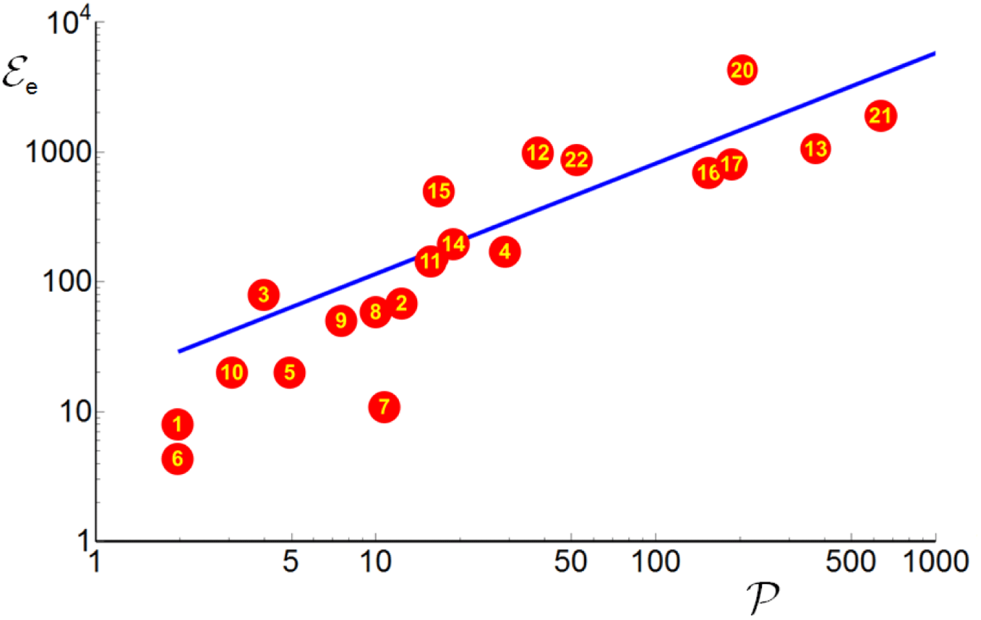
Figure 12. Experimental results on LWFA electron energy versus laser power (see Kando et al.
Reference Kando, Nakamura, Pirozhkov, Esirkepov, Koga and Bulanov2012). The indicated numbers correspond to the results reported as follows: 1 – Miura et al. (Reference Miura, Koyama, Kato, Saito, Adachi, Kawada, Nakamura and Tanimoto2005), 2 – Mangles et al. (Reference Mangles, Murphy, Najmudin, Thomas, Collier, Dangor, Divall, Foster, Gallacher and Hooker2004), 3 – Geddes et al. (Reference Geddes, Toth, van Tilborg, Esarey, Schroeder, Bruhwiler, Nieter, Cary and Leemans2004), 4 – Faure et al. (Reference Faure, Glinec, Pukhov, Kiselev, Gordienko, Lefebvre, Rousseau, Burgy and Malka2004), 5 – Yamazaki et al. (Reference Yamazaki, Kotaki, Daito, Kando, Bulanov, Esirkepov, Kondo, Kanazawa, Homma and Nakajima2005), 6 – Hafz et al. (Reference Hafz, Hur, Kim, Kim, Ko and Suk2006), 7 – Hosokai et al. (Reference Hosokai, Kinoshita, Ohkubo, Maekawa, Uesaka, Zhidkov, Yamazaki, Kotaki, Kando and Nakajima2006a
), 8 – Hsieh et al. (Reference Hsieh, Huang, Chang, Ho, Chen, Lin, Wang and Chen2006), 9 – Hidding et al. (Reference Hidding, Amthor, Liesfeld, Schwoerer, Karsch, Geissler, Veisz, Schmid, Gallacher and Jamison2006), 10 – Mori et al. (Reference Mori, Kando, Daito, Kotaki, Hayashi, Yamazaki, Ogura, Sagisaka, Koga and Nakajima2006), 11 – Mangles et al. (Reference Mangles, Thomas, Kaluza, Lundh, Lindau, Persson, Tsung, Najmudin, Mori and Wahlström2006), 12 – Leemans et al. (Reference Leemans, Nagler, Gonsalves, Toth, Nakamura, Geddes, Esarey, Schroeder and Hooker2006), 13 – Kameshima et al. (Reference Kameshima, Hong, Sugiyama, Wen, Wu, Tang, Zhu, Gu, Zhang and Peng2008), 14 – Hafz et al. (Reference Hafz, Jeong, Choi, Lee, Pae, Kulagin, Sung, Yu, Hong and Hosokai2008), 15 – Osterhoff et al. (Reference Osterhoff, Popp, Major, Marx, Rowlands-Rees, Fuchs, Geissler, Hörlein, Hidding and Becker2008), 16 – Karsch et al. (Reference Karsch, Osterhoff, Popp, Rowlands-Rees, Major, Fuchs, Marx, Hörlein, Schmid and Veisz2007), 17 – Kneip et al. (Reference Kneip, Nagel, Martins, Mangles, Bellei, Chekhlov, Clarke, Delerue, Divall and Doucas2009), 18 – Froula et al. (Reference Froula, Clayton, Döppner, Marsh, Barty, Divol, Fonseca, Glenzer, Joshi and Lu2009), 19 – Kim et al. (Reference Kim, Pae, Cha, Kim, Yu, Sung, Lee, Jeong and Lee2013), 20 – Leemans et al. (Reference Leemans, Gonsalves, Mao, Nakamura, Benedetti, Schroeder, Tóth, Daniels, Mittelberger and Bulanov2014), 21 – Wang et al. (Reference Wang, Zgadzaj, Fazel, Li, Yi, Zhang, Henderson, Chang, Korzekwa and Tsai2013), 22 – Walker et al. (Reference Walker, Bourgeois, Rittershofer, Cowley, Kajumba, Maier, Wenz, Werle, Karsch and Grüner2013). The fitting line corresponds to the dependence between the electron energy and laser power of the form
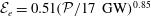 ${\mathcal{E}}_{e}=0.51({\mathcal{P}}/17~\text{GW})^{0.85}$
MeV.
${\mathcal{E}}_{e}=0.51({\mathcal{P}}/17~\text{GW})^{0.85}$
MeV.
The laser energy
 ${\mathcal{E}}_{las}$
required for acceleration of electrons up to the energy
${\mathcal{E}}_{las}$
required for acceleration of electrons up to the energy
 $m_{e}c^{2}{\it\gamma}_{e}$
can be found from the condition on the laser pulse length
$m_{e}c^{2}{\it\gamma}_{e}$
can be found from the condition on the laser pulse length
 $l_{las}$
to be equal to the optimal length
$l_{las}$
to be equal to the optimal length
 $l_{opt}(a)$
given by (2.21). Under this condition, the laser energy is
$l_{opt}(a)$
given by (2.21). Under this condition, the laser energy is
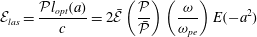 $$\begin{eqnarray}{\mathcal{E}}_{las}=\frac{{\mathcal{P}}l_{opt}(a)}{c}=2\bar{{\mathcal{E}}}\left(\frac{{\mathcal{P}}}{\bar{{\mathcal{P}}}}\right)\left(\frac{{\it\omega}}{{\it\omega}_{pe}}\right)E(-a^{2})\end{eqnarray}$$
with
 $$\begin{eqnarray}\bar{{\mathcal{E}}}=\frac{2{\rm\pi}\,\bar{{\mathcal{P}}}}{{\it\omega}}=\frac{4{\rm\pi}m_{e}^{2}c^{5}}{e^{2}{\it\omega}}\approx 33\left(\frac{{\it\lambda}}{1~{\rm\mu}\text{m}}\right){\rm\mu}\text{J}.\end{eqnarray}$$
In the case of the maximum of the accelerated electron energy given by (4.5), corresponding to the condition on the laser amplitude
 $a=1$
, the laser energy and power are related to each other as
$a=1$
, the laser energy and power are related to each other as
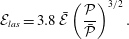 $$\begin{eqnarray}{\mathcal{E}}_{las}=3.8\,\bar{{\mathcal{E}}}\left(\frac{{\mathcal{P}}}{\bar{{\mathcal{P}}}}\right)^{3/2}.\end{eqnarray}$$
For example, with 1 PW power, a 1.8 KJ laser can accelerate electrons up to 30 GeV, and with 10 PW power, a 60 KJ laser can accelerate electrons up to 300 GeV. The required electron density,
 $n=n_{cr}/{\it\gamma}_{e,m}$
, with
$n=n_{cr}/{\it\gamma}_{e,m}$
, with
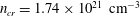 $n_{cr}=1.74\times 10^{21}~\text{cm}^{-3}$
for laser wavelength
$n_{cr}=1.74\times 10^{21}~\text{cm}^{-3}$
for laser wavelength
 ${\it\lambda}=800$
nm, is equal to
${\it\lambda}=800$
nm, is equal to
 ${\approx}3\times 10^{15}~\text{cm}^{-3}$
, in the first case of a 1 PW power, and to
${\approx}3\times 10^{15}~\text{cm}^{-3}$
, in the first case of a 1 PW power, and to
 ${\approx}3\times 10^{16}~\text{cm}^{-3}$
, in the case of a 10 PW power laser, respectively.
${\approx}3\times 10^{16}~\text{cm}^{-3}$
, in the case of a 10 PW power laser, respectively.
5 Unlimited acceleration regime with a tapered plasma target
The electron acceleration by the wake field excited in inhomogeneous plasma can be substantially enhanced. For matched laser–plasma parameters the electron acceleration can occur in an unlimited acceleration regime. This regime implies that the electron inside the wake wave does not leave the acceleration phase, i.e. the dephasing length is formally infinite, and its energy grows in time, being not limited asymptotically. The constant phase condition corresponds to the case when the gamma factor
 ${\it\gamma}_{w}$
calculated with the phase velocity of the wake wave remains equal to the electron Lorentz factor
${\it\gamma}_{w}$
calculated with the phase velocity of the wake wave remains equal to the electron Lorentz factor
 ${\it\gamma}_{e}$
during the electron interaction with the wake field. This condition can be realized when the laser pulse generates the wake wave in a downramp density plasma, where the laser pulse group velocity increases along the pulse propagation path which results in the increasing of the wake wave phase velocity and wavelength, providing constant acceleration phase conditions. Although the electric field decreases at this phase the integral of the electric field along the electron trajectory diverges, i.e. the energy gain formally is infinite. In figure 13 we illustrate the unlimited acceleration concept.
${\it\gamma}_{e}$
during the electron interaction with the wake field. This condition can be realized when the laser pulse generates the wake wave in a downramp density plasma, where the laser pulse group velocity increases along the pulse propagation path which results in the increasing of the wake wave phase velocity and wavelength, providing constant acceleration phase conditions. Although the electric field decreases at this phase the integral of the electric field along the electron trajectory diverges, i.e. the energy gain formally is infinite. In figure 13 we illustrate the unlimited acceleration concept.
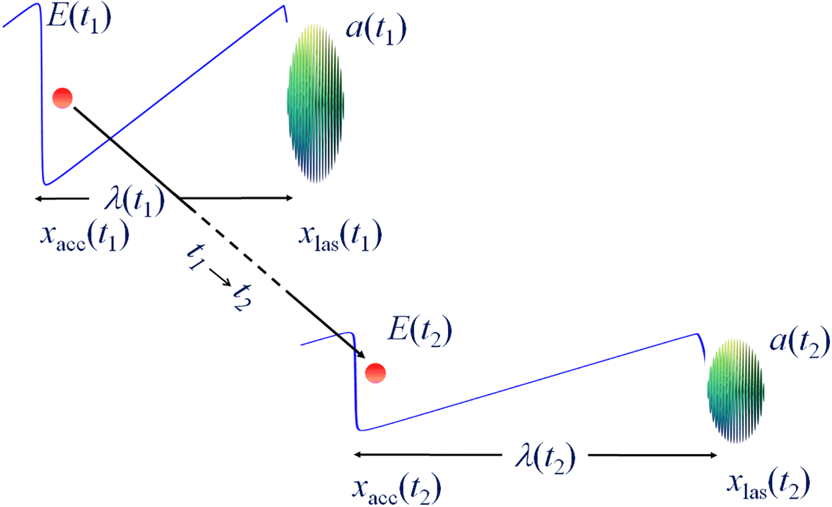
Figure 13. The wavelength and electric field amplitude changes being different at different times
 $t_{1}$
and
$t_{1}$
and
 $t_{2}$
due to the change of plasma density leading to a change in the laser pulse parameters. For a matched plasma density profile, the accelerated electrons remain in the acceleration phase of the wake field.
$t_{2}$
due to the change of plasma density leading to a change in the laser pulse parameters. For a matched plasma density profile, the accelerated electrons remain in the acceleration phase of the wake field.
Within the framework of the 1-D approximation, assuming that the wake wave is generated by an ultra-short laser pulse with constant amplitude
 $al_{las}\ll 1$
(see (2.27)–(2.32)), it has been shown in Bulanov et al. (Reference Bulanov, Vshivkov, Dudnikova, Naumova, Pegoraro and Pogorelsky1997b
) that in the plasma target with a downward gradient density
$al_{las}\ll 1$
(see (2.27)–(2.32)), it has been shown in Bulanov et al. (Reference Bulanov, Vshivkov, Dudnikova, Naumova, Pegoraro and Pogorelsky1997b
) that in the plasma target with a downward gradient density
 $n\sim x^{-2/3}$
the electron energy grows proportionally to
$n\sim x^{-2/3}$
the electron energy grows proportionally to
 ${\sim}x^{1/3}$
. The constant-amplitude condition can be satisfied, in particular, when the laser pulse is guided inside a constant radius waveguide filled by an inhomogeneous plasma. For laser pulse guiding, plasma filled capillaries have been extensively used (Ehrlich et al.
Reference Ehrlich, Cohen, Zigler, Krall, Sprangle and Esarey1996; Hosokai et al.
Reference Hosokai, Kando, Dewa, Kotaki, Kondo, Hasegawa, Nakajima and Horioka2000; Bobrova et al.
Reference Bobrova, Esaulov, Sakai, Sasorov, Spence, Butler, Hooker and Bulanov2001, Reference Bobrova, Sasorov, Benedetti, Bulanov, Geddes, Schroeder, Esarey and Leemans2013; Esarey et al.
Reference Esarey, Schroeder and Leemans2009; Kameshima et al.
Reference Kameshima, Kotaki, Kando, Daito, Kawase, Fukuda, Chen, Homma, Kondo and Esirkepov2009; Leemans et al.
Reference Leemans, Gonsalves, Mao, Nakamura, Benedetti, Schroeder, Tóth, Daniels, Mittelberger and Bulanov2014) as well as the channels produced in plasma by the ponderomotive force from picosecond pulses (Mizuta et al.
Reference Mizuta, Hosokai, Masuda, Zhidkov, Makito, Nakanii, Kajino, Nishida, Kando and Mori2012, Reference Mizuta, Hosokai, Masuda, Zhidkov, Nakanii, Jin, Nakahara, Kohara, Iwasa and Kando2016).
${\sim}x^{1/3}$
. The constant-amplitude condition can be satisfied, in particular, when the laser pulse is guided inside a constant radius waveguide filled by an inhomogeneous plasma. For laser pulse guiding, plasma filled capillaries have been extensively used (Ehrlich et al.
Reference Ehrlich, Cohen, Zigler, Krall, Sprangle and Esarey1996; Hosokai et al.
Reference Hosokai, Kando, Dewa, Kotaki, Kondo, Hasegawa, Nakajima and Horioka2000; Bobrova et al.
Reference Bobrova, Esaulov, Sakai, Sasorov, Spence, Butler, Hooker and Bulanov2001, Reference Bobrova, Sasorov, Benedetti, Bulanov, Geddes, Schroeder, Esarey and Leemans2013; Esarey et al.
Reference Esarey, Schroeder and Leemans2009; Kameshima et al.
Reference Kameshima, Kotaki, Kando, Daito, Kawase, Fukuda, Chen, Homma, Kondo and Esirkepov2009; Leemans et al.
Reference Leemans, Gonsalves, Mao, Nakamura, Benedetti, Schroeder, Tóth, Daniels, Mittelberger and Bulanov2014) as well as the channels produced in plasma by the ponderomotive force from picosecond pulses (Mizuta et al.
Reference Mizuta, Hosokai, Masuda, Zhidkov, Makito, Nakanii, Kajino, Nishida, Kando and Mori2012, Reference Mizuta, Hosokai, Masuda, Zhidkov, Nakanii, Jin, Nakahara, Kohara, Iwasa and Kando2016).
The phase velocity of the laser pulse propagating inside a plasma filled waveguide is determined by the waveguide transverse size and by the plasma density (see Benedetti et al. (Reference Benedetti, Rossi, Schroeder, Esarey and Leemans2015) for a detailed discussion of the laser pulse phase velocity dependence on the waveguide parameters). If the waveguide radius
 $R$
is small enough,
$R$
is small enough,
 $R\ll r_{c}=\sqrt{a}c/{\it\omega}_{pe}$
with
$R\ll r_{c}=\sqrt{a}c/{\it\omega}_{pe}$
with
 $k_{p}={\it\omega}_{pe}/c$
, the wake wave phase velocity is independent of the plasma density being determined by the waveguide radius with
$k_{p}={\it\omega}_{pe}/c$
, the wake wave phase velocity is independent of the plasma density being determined by the waveguide radius with
 ${\it\gamma}_{w}\approx kR$
, where
${\it\gamma}_{w}\approx kR$
, where
 $k_{0}={\it\omega}_{0}/c$
. For
$k_{0}={\it\omega}_{0}/c$
. For
 $R/r_{c}\gg 1$
we have
$R/r_{c}\gg 1$
we have
 ${\it\gamma}_{w}\approx k_{0}/k_{w}$
with
${\it\gamma}_{w}\approx k_{0}/k_{w}$
with
 $k_{w}=1/r_{c}$
. Figure 14 illustrates the wake wave excited inside a tapered waveguide.
$k_{w}=1/r_{c}$
. Figure 14 illustrates the wake wave excited inside a tapered waveguide.

Figure 14. Sketch of the wake wave excited inside a tapered waveguide.
5.1 High-amplitude limit
For given laser power the laser amplitude is higher the smaller the waveguide radius is. On the other hand, the smaller the channel radius is the lower the wake wave phase velocity is. Taking into account these constraints we assume that
 $$\begin{eqnarray}k_{w}R={\rm\pi},\end{eqnarray}$$
i.e. the channel diameter is equal to the wake wave wavelength. This condition gives a relationship between the plasma density and the channel radius.
We assume that the laser pulse excites a wake field inside the bubble with the radius
 $r_{c}=c\sqrt{a}{\it\omega}_{pe}$
. Its amplitude can be estimated to be equal to
$r_{c}=c\sqrt{a}{\it\omega}_{pe}$
. Its amplitude can be estimated to be equal to
 $$\begin{eqnarray}E_{w}=2{\rm\pi}en_{e}r_{c}=\frac{m_{e}c^{2}}{2e{\rm\pi}{\it\lambda}}\left(\frac{{\it\omega}_{pe}}{{\it\omega}}\right)^{2/3}\left(\frac{{\mathcal{P}}}{\bar{{\mathcal{P}}}}\right)^{1/6}.\end{eqnarray}$$
Here we have used the relationship between the laser pulse amplitude, power and plasma density given by (4.1). In the case of an inhomogeneous gas target for a given laser power the electromagnetic pulse amplitude depends on the plasma density according to relationship (4.1). For the normalized electron energy
 ${\it\gamma}_{e}$
we have the equation
${\it\gamma}_{e}$
we have the equation
 $$\begin{eqnarray}\frac{\text{d}{\it\gamma}_{e}}{\text{d}x}=\frac{eE_{w}}{m_{e}c^{2}}.\end{eqnarray}$$
Assuming that the accelerated electron Lorentz factor equals that calculated for the wake wave phase velocity,
 ${\it\gamma}_{e}={\it\gamma}_{w}$
, and taking into account that
${\it\gamma}_{e}={\it\gamma}_{w}$
, and taking into account that
 $$\begin{eqnarray}{\it\gamma}_{w}=\sqrt{a}\left(\frac{{\it\omega}}{{\it\omega}_{pe}}\right)=\left(\frac{{\mathcal{P}}}{\bar{{\mathcal{P}}}}\right)^{1/6}\left(\frac{{\it\omega}}{{\it\omega}_{pe}}\right)^{2/3}\end{eqnarray}$$
and
 $E_{w}=\sqrt{a}m_{e}c{\it\omega}_{pe}/e$
, we obtain a differential equation determining the electron density profile:
$E_{w}=\sqrt{a}m_{e}c{\it\omega}_{pe}/e$
, we obtain a differential equation determining the electron density profile:
 $$\begin{eqnarray}\frac{\text{d}}{\text{d}x}\left(\frac{{\it\omega}}{{\it\omega}_{pe}}\right)^{2/3}=\frac{{\rm\pi}}{{\it\lambda}}\left(\frac{{\it\omega}_{pe}}{{\it\omega}}\right)^{2/3}.\end{eqnarray}$$
Its solution gives
 $$\begin{eqnarray}n(x)=n_{cr}\left[\frac{4{\rm\pi}x}{3{\it\lambda}}+\left(\frac{{\it\omega}}{{\it\omega}_{pe}(0)}\right)^{4/3}\right]^{-3/2},\end{eqnarray}$$
where
 ${\it\omega}_{pe}(0)$
is the Langmuir frequency at
${\it\omega}_{pe}(0)$
is the Langmuir frequency at
 $x=0$
. The electron energy asymptotically grows in the regime of unlimited acceleration as
$x=0$
. The electron energy asymptotically grows in the regime of unlimited acceleration as
 $$\begin{eqnarray}{\it\gamma}_{e}(x)\approx \left(\frac{{\mathcal{P}}}{\bar{{\mathcal{P}}}}\right)^{1/6}\left(\frac{4{\rm\pi}x}{3{\it\lambda}}\right)^{1/2}.\end{eqnarray}$$
From (5.1), (4.1) and (5.6) it follows that the radius of the tapered channel should linearly depend on the coordinate
 $x$
,
$x$
,
 $$\begin{eqnarray}R(x)=\frac{{\it\lambda}}{2}\left(\frac{{\mathcal{P}}}{\bar{{\mathcal{P}}}}\right)^{1/6}\left[\frac{4{\rm\pi}x}{3{\it\lambda}}+\left(\frac{{\it\omega}}{{\it\omega}_{pe}(0)}\right)^{4/3}\right].\end{eqnarray}$$
5.2 Short pulse driver laser
Since it is difficult to keep the optimal length of the laser pulse when it propagates in an inhomogeneous plasma, we shall consider here the case of a short pulse laser, i.e.
 $a^{2}l_{las}\ll 1$
. The wake-field amplitude and wavelength are given by (2.27) and (2.29), respectively. In dimensional units, the wake-field amplitude is equal to
$a^{2}l_{las}\ll 1$
. The wake-field amplitude and wavelength are given by (2.27) and (2.29), respectively. In dimensional units, the wake-field amplitude is equal to
 $$\begin{eqnarray}E_{w}=\frac{m_{e}{\it\omega}_{pe}^{2}}{2e}a^{2}l_{las}\end{eqnarray}$$
and the wake wave wavelength is
 $2l_{las}a^{2}$
. This approximation implies that the laser power is below threshold of relativistic self-focusing, i.e.
$2l_{las}a^{2}$
. This approximation implies that the laser power is below threshold of relativistic self-focusing, i.e.
 ${\mathcal{P}}/\bar{{\mathcal{P}}}<n_{cr}/n$
. Assuming that the waveguide radius is of the order of
${\mathcal{P}}/\bar{{\mathcal{P}}}<n_{cr}/n$
. Assuming that the waveguide radius is of the order of
 $c/{\it\omega}_{pe}$
we obtain for the normalized laser pulse amplitude
$c/{\it\omega}_{pe}$
we obtain for the normalized laser pulse amplitude
 $$\begin{eqnarray}a^{2}=\frac{{\mathcal{P}}}{\bar{{\mathcal{P}}}}\left(\frac{{\it\omega}_{pe}}{{\it\omega}}\right)^{2}\end{eqnarray}$$
and the wake-field amplitude
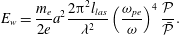 $$\begin{eqnarray}E_{w}=\frac{m_{e}}{2e}a^{2}\frac{2{\rm\pi}^{2}l_{las}}{{\it\lambda}^{2}}\left(\frac{{\it\omega}_{pe}}{{\it\omega}}\right)^{4}\frac{{\mathcal{P}}}{\bar{{\mathcal{P}}}}.\end{eqnarray}$$
Using equation (5.3) with
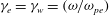 ${\it\gamma}_{e}={\it\gamma}_{w}=({\it\omega}/{\it\omega}_{pe})$
and the electric field on the right-hand side given by (5.11), we write the differential equation for the plasma density profile as
${\it\gamma}_{e}={\it\gamma}_{w}=({\it\omega}/{\it\omega}_{pe})$
and the electric field on the right-hand side given by (5.11), we write the differential equation for the plasma density profile as
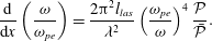 $$\begin{eqnarray}\frac{\text{d}}{\text{d}x}\left(\frac{{\it\omega}}{{\it\omega}_{pe}}\right)=\frac{2{\rm\pi}^{2}l_{las}}{{\it\lambda}^{2}}\left(\frac{{\it\omega}_{pe}}{{\it\omega}}\right)^{4}\frac{{\mathcal{P}}}{\bar{{\mathcal{P}}}}.\end{eqnarray}$$
The solution of this equation gives the plasma density dependence on the coordinate
 $x$
$x$
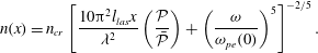 $$\begin{eqnarray}n(x)=n_{cr}\left[\frac{10{\rm\pi}^{2}l_{las}x}{{\it\lambda}^{2}}\left(\frac{{\mathcal{P}}}{\bar{{\mathcal{P}}}}\right)+\left(\frac{{\it\omega}}{{\it\omega}_{pe}(0)}\right)^{5}\right]^{-2/5}.\end{eqnarray}$$
The gamma factor of accelerated electrons asymptotically grows with the coordinate
 $x$
in this regime of unlimited acceleration as
$x$
in this regime of unlimited acceleration as
 $$\begin{eqnarray}{\it\gamma}_{e}(x)\approx \left[\frac{10{\rm\pi}^{2}l_{las}x}{{\it\lambda}^{2}}\left(\frac{{\mathcal{P}}}{\bar{{\mathcal{P}}}}\right)\right]^{1/5}.\end{eqnarray}$$
Using the relationships obtained we can find that the radius of the tapered channel should depend on the coordinate proportional to
 $x^{1/5}$
,
$x^{1/5}$
,
 $$\begin{eqnarray}R(x)={\it\lambda}\left[\frac{10{\rm\pi}^{2}l_{las}x}{{\it\lambda}^{2}}\left(\frac{{\mathcal{P}}}{\bar{{\mathcal{P}}}}\right)+\left(\frac{{\it\omega}}{{\it\omega}_{pe}(0)}\right)^{5}\right]^{1/5}.\end{eqnarray}$$
6 Electron beam dynamics inside the cavity
One of the limits on the LFWA operation is due to the effects produced by the electromagnetic field of the accelerated electron bunch (Esarey et al. Reference Esarey, Schroeder and Leemans2009). When the electric charge of the accelerated electrons is high enough to produce an electric field of the order of the electric field inside the cavity, in an uncontrollable regime the quality of the accelerated electron bunch deteriorates, although when the bunch is carefully shaped, the total electric field can be made constant over the bunch length, which minimizes the energy spread (Wilks et al. Reference Wilks, Katsouleas, Dawson, Chen and Su1987; Tzoufras et al. Reference Tzoufras, Lu, Tsung, Huang, Mori, Katsouleas, Vieira, Fonseca and Silva2008). The problem of beam loading has been addressed experimentally and theoretically in a number of works, e. g. see Rechatin et al. (Reference Rechatin, Davoine, Lifschitz, Ismail, Lim, Lefebvre, Faure and Malka2009a ), Guillaume et al. (Reference Guillaume, Döpp, Thaury, Lifschitz, Goddet, Tafzi, Sylla, Iaquanello, Lefrou and Rousseau2015a ) and the review article Esarey et al. (Reference Esarey, Schroeder and Leemans2009) and references therein. The beam overloading constraint imposes an upper limit on the number of accelerated particles. The latter is crucial for various applications of LFWA accelerators.

Figure 15. Electron bunch of radius
 $R^{(b)}$
inside a cavity of radius
$R^{(b)}$
inside a cavity of radius
 $r_{c}$
.
$r_{c}$
.
Here we consider the electron bunch equilibrium and oscillation around equilibrium inside the wake when its transverse size is substantially smaller than its length, assuming that the longitudinal scale length (along the
 $x$
axis) of the fast electron bunch is much greater than its scale length in the transverse direction (see figure 15 and Kando et al. (Reference Kando, Fukuda, Kotaki, Koga, Bulanov, Tajima, Chao, Pitthan, Schuler and Zhidkov2007)). Such an approximation may be valid in the near-axis region of the wake when the injection time is of the order of the electron acceleration time.
$x$
axis) of the fast electron bunch is much greater than its scale length in the transverse direction (see figure 15 and Kando et al. (Reference Kando, Fukuda, Kotaki, Koga, Bulanov, Tajima, Chao, Pitthan, Schuler and Zhidkov2007)). Such an approximation may be valid in the near-axis region of the wake when the injection time is of the order of the electron acceleration time.
6.1 Equations of motion
The equations of the motion of a fluid element of the electron bunch in the transverse direction are
 $$\begin{eqnarray}\partial _{t}n^{(b)}+\frac{1}{r}\partial _{r}(n^{(b)}v_{r}^{(b)})=0,\end{eqnarray}$$
for the beam density
 $n^{(b)}(t,r)$
, and
$n^{(b)}(t,r)$
, and
 $$\begin{eqnarray}\displaystyle & \displaystyle \partial _{t}p_{r}^{(b)}+v_{r}^{(b)}\partial _{r}p_{r}^{(b)}-\frac{v_{{\it\theta}}^{(b)}p_{{\it\theta}}^{(b)}}{r}=-e\left(E_{r}+\frac{v_{x}^{(b)}}{c}B_{{\it\theta}}-\frac{v_{{\it\theta}}^{(b)}}{c}B_{x}\right), & \displaystyle\end{eqnarray}$$
 $$\begin{eqnarray}\displaystyle & \displaystyle \partial _{t}p_{{\it\theta}}^{(b)}+v_{r}^{(b)}\partial _{r}p_{{\it\theta}}^{(b)}+\frac{v_{r}^{(b)}p_{{\it\theta}}^{(b)}}{r}=-e\frac{v_{r}^{(b)}}{c}B_{x}, & \displaystyle\end{eqnarray}$$
for the radial and azimuthal components of the beam momentum, respectively. The subscript
 $(b)$
stands for the functions describing the beam. The beam momentum components are related to the components of the beam velocity as
$(b)$
stands for the functions describing the beam. The beam momentum components are related to the components of the beam velocity as
 $p_{r}^{(b)}={\it\gamma}^{(b)}m_{e}v_{r}^{(b)}$
and
$p_{r}^{(b)}={\it\gamma}^{(b)}m_{e}v_{r}^{(b)}$
and
 $p_{{\it\theta}}^{(b)}={\it\gamma}^{(b)}m_{e}v_{{\it\theta}}^{(b)}$
and
$p_{{\it\theta}}^{(b)}={\it\gamma}^{(b)}m_{e}v_{{\it\theta}}^{(b)}$
and
 $v_{x}^{(b)}=c{\it\beta}^{(b)}$
is the beam velocity in the
$v_{x}^{(b)}=c{\it\beta}^{(b)}$
is the beam velocity in the
 $x$
direction. We introduce the associated gamma factor,
$x$
direction. We introduce the associated gamma factor,
 $$\begin{eqnarray}{\it\gamma}^{(b)}=1/\sqrt{1-{\it\beta}^{(b)\,2}},\end{eqnarray}$$
with
 ${\it\beta}^{(b)}=v_{x}^{(b)}/c$
corresponding to the beam velocity along the direction of the laser pulse propagation. Here and below in this subsection we assume
${\it\beta}^{(b)}=v_{x}^{(b)}/c$
corresponding to the beam velocity along the direction of the laser pulse propagation. Here and below in this subsection we assume
 $v_{x}^{(b)}$
to be constant, which implies that the
$v_{x}^{(b)}$
to be constant, which implies that the
 $x$
-component of the electron momentum
$x$
-component of the electron momentum
 $p_{x}^{(b)}=m_{e}v_{x}^{(b)}{\it\gamma}^{(b)}$
is substantially larger than the momentum transverse components,
$p_{x}^{(b)}=m_{e}v_{x}^{(b)}{\it\gamma}^{(b)}$
is substantially larger than the momentum transverse components,
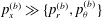 $p_{x}^{(b)}\gg \{p_{r}^{(b)},p_{{\it\theta}}^{(b)}\}$
, which corresponds to the well-known betatron approximation (Humphries Reference Humphries1990).
$p_{x}^{(b)}\gg \{p_{r}^{(b)},p_{{\it\theta}}^{(b)}\}$
, which corresponds to the well-known betatron approximation (Humphries Reference Humphries1990).
The electric field in the right-hand side of (6.2) is a sum of the radial component of the electric field inside the cavity
 $2{\rm\pi}n_{0}er$
produced by positively charged ion background and of the electric field of the electron beam
$2{\rm\pi}n_{0}er$
produced by positively charged ion background and of the electric field of the electron beam
 $E_{r}^{(b)}$
, which is governed by equation
$E_{r}^{(b)}$
, which is governed by equation
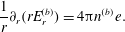 $$\begin{eqnarray}\frac{1}{r}\partial _{r}(rE_{r}^{(b)})=4{\rm\pi}n^{(b)}e.\end{eqnarray}$$
The magnetic field
 $\boldsymbol{B}=B_{x}\boldsymbol{e}_{x}+B_{{\it\theta}}\boldsymbol{e}_{{\it\theta}}$
is a combination of an external magnetic field
$\boldsymbol{B}=B_{x}\boldsymbol{e}_{x}+B_{{\it\theta}}\boldsymbol{e}_{{\it\theta}}$
is a combination of an external magnetic field
 $B_{x}\boldsymbol{e}_{x}$
directed along the laser pulse propagation and the magnetic field produced by the electric current carried by the electron beam
$B_{x}\boldsymbol{e}_{x}$
directed along the laser pulse propagation and the magnetic field produced by the electric current carried by the electron beam
 $B_{{\it\theta}}\boldsymbol{e}_{{\it\theta}}$
. Here
$B_{{\it\theta}}\boldsymbol{e}_{{\it\theta}}$
. Here
 $\boldsymbol{e}_{x}$
and
$\boldsymbol{e}_{x}$
and
 $\boldsymbol{e}_{{\it\theta}}$
are the unit vectors in the
$\boldsymbol{e}_{{\it\theta}}$
are the unit vectors in the
 $x$
and
$x$
and
 ${\it\theta}$
directions.
${\it\theta}$
directions.
An axial magnetic field
 $B_{x}\boldsymbol{e}_{x}$
can be generated by the circularly polarized laser radiation via the inverse Faraday effect and/or it can be externally imposed. Strong magnetic fields can change the whole scenario of the laser plasma interaction (Askar’yan et al.
Reference Askar’yan, Bulanov, Pegoraro and Pukhov1994; Pukhov & Meyer-ter Vehn Reference Pukhov and Meyer-ter Vehn1996; Bulanov et al.
Reference Bulanov, Zh. Esirkepov, Kando, Koga, Hosokai, Zhidkov and Kodama2013b
; Rassou, Bourdier & Drouin Reference Rassou, Bourdier and Drouin2015) and, in particular, they modify the charged particle acceleration by electrostatic waves Katsouleas & Dawson (Reference Katsouleas and Dawson1983), Bulanov & Sakharov (Reference Bulanov and Sakharov1986), Berezinskii et al. (Reference Berezinskii, Bulanov, Ginzburg, Dogiel and Ptuskin1990), Dieckmann, Shukla & Drury (Reference Dieckmann, Shukla and Drury2008), Neishtadt et al. (Reference Neishtadt, Artemyev, Zelenyi and Vainshtein2009) and injection (Vieira et al.
Reference Vieira, Martins, Pathak, Fonseca, Mori and Silva2011, Reference Vieira, Martins, Pathak, Fonseca, Mori and Silva2012). An externally imposed homogeneous magnetic field can significantly improve the quality and stability of laser wake-field accelerated electrons (Hosokai et al.
Reference Hosokai, Kinoshita, Zhidkov, Maekawa, Yamazaki and Uesaka2006b
, Reference Hosokai, Zhidkov, Yamazaki, Mizuta, Uesaka and Kodama2010). Below we assume that an axial magnetic field is given.
$B_{x}\boldsymbol{e}_{x}$
can be generated by the circularly polarized laser radiation via the inverse Faraday effect and/or it can be externally imposed. Strong magnetic fields can change the whole scenario of the laser plasma interaction (Askar’yan et al.
Reference Askar’yan, Bulanov, Pegoraro and Pukhov1994; Pukhov & Meyer-ter Vehn Reference Pukhov and Meyer-ter Vehn1996; Bulanov et al.
Reference Bulanov, Zh. Esirkepov, Kando, Koga, Hosokai, Zhidkov and Kodama2013b
; Rassou, Bourdier & Drouin Reference Rassou, Bourdier and Drouin2015) and, in particular, they modify the charged particle acceleration by electrostatic waves Katsouleas & Dawson (Reference Katsouleas and Dawson1983), Bulanov & Sakharov (Reference Bulanov and Sakharov1986), Berezinskii et al. (Reference Berezinskii, Bulanov, Ginzburg, Dogiel and Ptuskin1990), Dieckmann, Shukla & Drury (Reference Dieckmann, Shukla and Drury2008), Neishtadt et al. (Reference Neishtadt, Artemyev, Zelenyi and Vainshtein2009) and injection (Vieira et al.
Reference Vieira, Martins, Pathak, Fonseca, Mori and Silva2011, Reference Vieira, Martins, Pathak, Fonseca, Mori and Silva2012). An externally imposed homogeneous magnetic field can significantly improve the quality and stability of laser wake-field accelerated electrons (Hosokai et al.
Reference Hosokai, Kinoshita, Zhidkov, Maekawa, Yamazaki and Uesaka2006b
, Reference Hosokai, Zhidkov, Yamazaki, Mizuta, Uesaka and Kodama2010). Below we assume that an axial magnetic field is given.
The magnetic field produced by the electric current carried by of the electron beam should be found from equation
 $$\begin{eqnarray}\frac{1}{r}\partial _{r}(rB_{{\it\theta}}^{(b)})=4{\rm\pi}n_{b}e{\it\beta}^{(b)}.\end{eqnarray}$$
To solve the system of equations (6.1)–(6.6) it is convenient to use the Lagrange variables
 $t^{\prime }$
,
$t^{\prime }$
,
 $r_{0}$
related to the Euler variables
$r_{0}$
related to the Euler variables
 $t$
,
$t$
,
 $r$
as
$r$
as
 $$\begin{eqnarray}t^{\prime }=t\quad \text{and}\quad r=r_{0}+{\it\rho}(t,r_{0}),\end{eqnarray}$$
where the Lagrange coordinate
 $r_{0}$
is chosen to be the initial (
$r_{0}$
is chosen to be the initial (
 $t=0$
) coordinate of the element of the electron fluid with
$t=0$
) coordinate of the element of the electron fluid with
 ${\it\rho}(t,r_{0})$
being the electron displacement from the initial position.
${\it\rho}(t,r_{0})$
being the electron displacement from the initial position.
The solution of the continuity equation (6.1) is given by
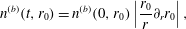 $$\begin{eqnarray}n^{(b)}(t,r_{0})=n^{(b)}(0,r_{0})\left|\frac{r_{0}}{r}\partial _{r}r_{0}\right|,\end{eqnarray}$$
which can be written in the form
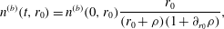 $$\begin{eqnarray}n^{(b)}(t,r_{0})=n^{(b)}(0,r_{0})\frac{r_{0}}{(r_{0}+{\it\rho})(1+\partial _{r_{0}}{\it\rho})},\end{eqnarray}$$
where
 $(r_{0}/r)\partial _{r_{0}}r$
equal to
$(r_{0}/r)\partial _{r_{0}}r$
equal to
 $r_{0}/[(r_{0}+{\it\rho})(1+\partial _{r_{0}}{\it\rho})]$
in the right-hand side of (6.8) and (6.9) is the Jacobian of the transformation from the Euler to Lagrange coordinates. The function
$r_{0}/[(r_{0}+{\it\rho})(1+\partial _{r_{0}}{\it\rho})]$
in the right-hand side of (6.8) and (6.9) is the Jacobian of the transformation from the Euler to Lagrange coordinates. The function
 $n^{(b)}(0,r_{0})$
gives the electron density distribution at
$n^{(b)}(0,r_{0})$
gives the electron density distribution at
 $t=0$
.
$t=0$
.
From (6.1), (6.5) and (6.6) we obtain that the electric and magnetic field produced by the bunch depend on the variables
 $t$
and
$t$
and
 $r_{0}$
as
$r_{0}$
as
 $$\begin{eqnarray}E_{r}^{(b)}(t,r_{0})=\frac{2e\mathbb{N}^{(b)}(r_{0})}{r_{0}+{\it\rho}}\end{eqnarray}$$
and
 $$\begin{eqnarray}B_{{\it\theta}}^{(b)}=\frac{2e\mathbb{N}^{(b)}(r_{0}){\it\beta}^{(b)}}{r_{0}+{\it\rho}},\end{eqnarray}$$
respectively. As we see, there is a relationship,
 $B_{{\it\theta}}^{(b)}={\it\beta}^{(b)}E_{{\it\theta}}^{(b)}$
between the beam generated electric and magnetic fields. In (6.10) and (6.11),
$B_{{\it\theta}}^{(b)}={\it\beta}^{(b)}E_{{\it\theta}}^{(b)}$
between the beam generated electric and magnetic fields. In (6.10) and (6.11),
 $\mathbb{N}^{(b)}(r_{0})$
is the electron number within the radius
$\mathbb{N}^{(b)}(r_{0})$
is the electron number within the radius
 $r_{0}$
per unit length in the bunch. It is equal to the integral over the surface of the radius
$r_{0}$
per unit length in the bunch. It is equal to the integral over the surface of the radius
 $r_{0}$
 $$\begin{eqnarray}\mathbb{N}^{(b)}(r_{0})=2{\rm\pi}\int _{0}^{r_{0}}n^{(b)}(0,s)s\,\text{d}s.\end{eqnarray}$$
Integration of equation (6.3) written in the Lagrange variables,
 $$\begin{eqnarray}{\dot{p}}_{{\it\theta}}^{(b)}+\frac{v_{r}^{(b)}p_{{\it\theta}}^{(b)}}{r_{0}+{\it\rho}}=\frac{e}{c}v_{r}^{(b)}B_{x},\end{eqnarray}$$
results in the dependence of the
 ${\it\theta}$
component of the electron momentum on
${\it\theta}$
component of the electron momentum on
 $r_{0},t$
 $$\begin{eqnarray}(r_{0}+{\it\rho}(r_{0},t))p_{{\it\theta}}^{(b)}(r_{0},t)=\frac{e}{2c}(r_{0}+{\it\rho}(r_{0},t))^{2}B_{x}+\mathbb{M}_{{\it\theta}}^{(b)}(r_{0}),\end{eqnarray}$$
with the function
 $\mathbb{M}_{{\it\theta}}^{(b)}(r_{0})$
determined by the initial distribution of the angular momentum inside the bunch. Here and below a dot stands for differentiation with respect to time. We have used the fact that the radial component of the beam velocity in Lagrange variables is equal to the partial derivative of the radial coordinate on time,
$\mathbb{M}_{{\it\theta}}^{(b)}(r_{0})$
determined by the initial distribution of the angular momentum inside the bunch. Here and below a dot stands for differentiation with respect to time. We have used the fact that the radial component of the beam velocity in Lagrange variables is equal to the partial derivative of the radial coordinate on time,
 $v_{r}^{(b)}=\partial _{t}{\it\rho}$
. The integral (6.14) stems from the conservation of total angular momentum in electrodynamics.
$v_{r}^{(b)}=\partial _{t}{\it\rho}$
. The integral (6.14) stems from the conservation of total angular momentum in electrodynamics.
Substituting the relationships obtained to (6.2) written into the Lagrange variables we obtain it as
 $$\begin{eqnarray}\ddot{r}+{\it\omega}_{UH}^{2}r=\frac{\mathbb{M}_{{\it\theta}}^{(b)\,2}(r_{0})}{m_{e}^{2}{\it\gamma}^{(b)}r^{3}}+\frac{2e^{2}\mathbb{N}^{(b)}(r_{0})}{m_{e}{\it\gamma}^{(b)\,3}r},\end{eqnarray}$$
where
 $r(r_{0},t)=r_{0}+{\it\rho}(r_{0},t)$
is the radius of the electron fluid element located initially at
$r(r_{0},t)=r_{0}+{\it\rho}(r_{0},t)$
is the radius of the electron fluid element located initially at
 $r_{0}$
and
$r_{0}$
and
 $$\begin{eqnarray}{\it\omega}_{UH}^{2}=\frac{{\it\omega}_{pe}^{2}}{2{\it\gamma}^{(b)}}+\frac{{\it\omega}_{Be}^{2}}{4{\it\gamma}^{(b)}}\end{eqnarray}$$
is the square of the frequency of betatron oscillations of a single electron moving inside the wake-field cavity in the presence of the magnetic field
 $B_{x}\boldsymbol{e}_{x}$
. The frequency
$B_{x}\boldsymbol{e}_{x}$
. The frequency
 ${\it\omega}_{pe}/\sqrt{2{\it\gamma}^{(b)}}$
is the frequency of betatron oscillations in the case of zero axial magnetic field (for details see review article Corde et al.
Reference Corde, Thaury, Lifschitz, Lambert, Ta Phuoc, Davoine, Lehe, Douillet, Rousse and Malka2013). The frequency
${\it\omega}_{pe}/\sqrt{2{\it\gamma}^{(b)}}$
is the frequency of betatron oscillations in the case of zero axial magnetic field (for details see review article Corde et al.
Reference Corde, Thaury, Lifschitz, Lambert, Ta Phuoc, Davoine, Lehe, Douillet, Rousse and Malka2013). The frequency
 ${\it\omega}_{Be}=eB_{x}/m_{e}c$
is the Larmor frequency for an electron in magnetic field
${\it\omega}_{Be}=eB_{x}/m_{e}c$
is the Larmor frequency for an electron in magnetic field
 $B_{x}$
.
$B_{x}$
.
The equation (6.15) has a form similar to the Kapchinskij–Vladimirskij equation (Kapchinskij & Vladimirskij Reference Kapchinskij and Vladimirskij1959) for the particle beam envelope. The Kapchinskij–Vladimirskij equation is well known in the theory of standard accelerators of charged particles (e.g. see Chao Reference Chao1993). It has also been used in Bulanov, Mourou & Tajima (Reference Bulanov, Mourou and Tajima2008a ) to describe the relativistic electron slicing by a wake field excited in laser plasma.
The term
 $\mathbb{M}_{{\it\theta}}^{(b)\,2}(r_{0})/m_{e}{\it\gamma}^{(b)}$
on the right-hand side of (6.15) describing the effects of the electron momentum is proportional to the square of the transverse emittance of the bunch. The last term on the right-hand side of (6.15) describes space charge effects.
$\mathbb{M}_{{\it\theta}}^{(b)\,2}(r_{0})/m_{e}{\it\gamma}^{(b)}$
on the right-hand side of (6.15) describing the effects of the electron momentum is proportional to the square of the transverse emittance of the bunch. The last term on the right-hand side of (6.15) describes space charge effects.
We note here, that if the wake wave is excited in a transversally inhomogeneous plasma with density
 $n_{0}(r)$
, e.g. when the laser pulse driver propagates inside the capillary wave guide, the second term on the left-hand side should be
$n_{0}(r)$
, e.g. when the laser pulse driver propagates inside the capillary wave guide, the second term on the left-hand side should be
 $$\begin{eqnarray}\frac{4{\rm\pi}e^{2}}{m_{e}{\it\gamma}^{(b)}(r_{0}+{\it\rho})}\int _{0}^{r_{0}+{\it\rho}}n_{0}(s)\,s\,\text{d}s.\end{eqnarray}$$
Equation (6.15) describes the finite-amplitude betatron oscillations of the electron bunch around the equilibrium. In a transversally inhomogeneous plasma the nonlinear dependence of the frequency on the radius via (6.17) should result in the so-called phase-mixing phenomenon.
6.2 Equilibrium
At the equilibrium (
 ${\it\rho}=0$
) (6.15) yields
${\it\rho}=0$
) (6.15) yields
 $$\begin{eqnarray}{\it\omega}_{UH}^{2}r^{(b)\,4}-\frac{2e^{2}\mathbb{N}^{(b)}(r^{(b)})}{m_{e}{\it\gamma}^{(b)\,3}}r^{(b)\,2}-\frac{\mathbb{M}_{{\it\theta}}^{(b)\,2}(r^{(b)})}{m_{e}^{2}{\it\gamma}^{(b)}}=0,\end{eqnarray}$$
where
 $r^{(b)}$
is the coordinate of the electron fluid layer. If the angular momentum
$r^{(b)}$
is the coordinate of the electron fluid layer. If the angular momentum
 $\mathbb{M}^{(b)}(R^{(b)})$
and the number of particles
$\mathbb{M}^{(b)}(R^{(b)})$
and the number of particles
 $\mathbb{N}^{(b)}(R^{(b)})$
are given parameters characterizing the electron bunch of the radius
$\mathbb{N}^{(b)}(R^{(b)})$
are given parameters characterizing the electron bunch of the radius
 $R^{(b)}$
(this is the outermost radial coordinate of the electrons), then (6.18) is the algebraic quadratic equation for the bunch radius
$R^{(b)}$
(this is the outermost radial coordinate of the electrons), then (6.18) is the algebraic quadratic equation for the bunch radius
 $r^{(b)}=R^{(b)}$
. As a result we find that the bunch radius is equal to
$r^{(b)}=R^{(b)}$
. As a result we find that the bunch radius is equal to
 $$\begin{eqnarray}R^{(b)}=\sqrt{\left(\frac{e^{2}\mathbb{ N}^{(b)}}{m_{e}{\it\gamma}^{(b)\,3}{\it\omega}_{UH}^{2}}\right)\left(1+\sqrt{1+\frac{\mathbb{ M}_{{\it\theta}}^{(b)\,2}{\it\gamma}^{(b)\,5}{\it\omega}_{UH}^{2}}{e^{4}\mathbb{N}^{(b)\,2}}}\right)}.\end{eqnarray}$$
If the electron density
 $n^{(b)}$
is homogeneous inside the bunch, and and the angular momentum distribution corresponds to the rigid rotation of the bunch with constant angular frequency
$n^{(b)}$
is homogeneous inside the bunch, and and the angular momentum distribution corresponds to the rigid rotation of the bunch with constant angular frequency
 ${\it\Omega}^{(b)}$
, then the total number of particles and angular momentum,
${\it\Omega}^{(b)}$
, then the total number of particles and angular momentum,
 $$\begin{eqnarray}\mathbb{N}^{(b)}={\rm\pi}n^{(b)}R^{(b)\,2}\quad \text{and}\quad \mathbb{M}_{{\it\theta}}^{(b)}=m_{e}{\it\Omega}^{(b)}R^{(b)\,2},\end{eqnarray}$$
are proportional to square of the radius
 $R^{(b)}$
. In this case, from (6.18) it follows that at equilibrium the electron bunch density equals
$R^{(b)}$
. In this case, from (6.18) it follows that at equilibrium the electron bunch density equals
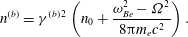 $$\begin{eqnarray}n^{(b)}={\it\gamma}^{(b)\,2}\left(n_{0}+\frac{{\it\omega}_{Be}^{2}-{\it\Omega}^{2}}{8{\rm\pi}m_{e}c^{2}}\right).\end{eqnarray}$$
As we see, for zero magnetic field,
 $B_{x}=0$
, and a non-rotating bunch with
$B_{x}=0$
, and a non-rotating bunch with
 ${\it\Omega}=0$
the equilibrium bunch density is a factor
${\it\Omega}=0$
the equilibrium bunch density is a factor
 ${\it\gamma}^{(b)\,2}$
higher than the background plasma density
${\it\gamma}^{(b)\,2}$
higher than the background plasma density
 $n_{0}$
. A strong enough magnetic field (
$n_{0}$
. A strong enough magnetic field (
 ${\it\omega}_{Be}/{\it\omega}_{pe}\gg 1$
) and fast enough rotation (
${\it\omega}_{Be}/{\it\omega}_{pe}\gg 1$
) and fast enough rotation (
 ${\it\Omega}/{\it\omega}_{pe}\gg 1$
) can significantly either increase for
${\it\Omega}/{\it\omega}_{pe}\gg 1$
) can significantly either increase for
 ${\it\omega}_{Be}^{2}>{\it\Omega}^{2}$
or decrease the electron bunch density, if
${\it\omega}_{Be}^{2}>{\it\Omega}^{2}$
or decrease the electron bunch density, if
 ${\it\omega}_{Be}^{2}<{\it\Omega}^{2}$
. The equilibrium radius
${\it\omega}_{Be}^{2}<{\it\Omega}^{2}$
. The equilibrium radius
 $R^{(b)}$
can accordingly be smaller in the case
$R^{(b)}$
can accordingly be smaller in the case
 ${\it\omega}_{Be}^{2}>{\it\Omega}^{2}$
or larger if
${\it\omega}_{Be}^{2}>{\it\Omega}^{2}$
or larger if
 ${\it\omega}_{Be}^{2}<{\it\Omega}^{2}$
. In turn a smaller bunch radius implies relatively narrower energy spectrum of accelerated electrons because they see locally a more homogeneous accelerating electric field.
${\it\omega}_{Be}^{2}<{\it\Omega}^{2}$
. In turn a smaller bunch radius implies relatively narrower energy spectrum of accelerated electrons because they see locally a more homogeneous accelerating electric field.
6.3 The
$m=0$
betatron oscillations

The ordinary differential equation (6.15) has an integral
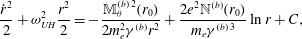 $$\begin{eqnarray}\frac{{\dot{r}}^{2}}{2}+{\it\omega}_{UH}^{2}\frac{r^{2}}{2}=-\frac{\mathbb{M}_{{\it\theta}}^{(b)\,2}(r_{0})}{2m_{e}^{2}{\it\gamma}^{(b)}r^{2}}+\frac{2e^{2}\mathbb{N}^{(b)}(r_{0})}{m_{e}{\it\gamma}^{(b)\,3}}\ln r+C,\end{eqnarray}$$
where the constant
 $C$
is determined by the initial conditions
$C$
is determined by the initial conditions
 $r_{0}$
and
$r_{0}$
and
 ${\dot{r}}_{0}$
. Equation (6.15), taking into account the integral (6.22), describes nonlinear betatron oscillations.
${\dot{r}}_{0}$
. Equation (6.15), taking into account the integral (6.22), describes nonlinear betatron oscillations.
Linearizing (6.15) around the equilibrium given by (6.19), i.e. assuming
 $r=R^{(b)}+{\it\delta}r(t)$
with
$r=R^{(b)}+{\it\delta}r(t)$
with
 ${\it\delta}r/R^{(b)}\ll 1$
, we obtain a linear ordinary differential equation for the function
${\it\delta}r/R^{(b)}\ll 1$
, we obtain a linear ordinary differential equation for the function
 ${\it\delta}r(r_{0},t)$
. It describes the radial oscillations of the electron bunch (such a mode is called the
${\it\delta}r(r_{0},t)$
. It describes the radial oscillations of the electron bunch (such a mode is called the
 $m=0$
mode) with frequency
$m=0$
mode) with frequency
 $$\begin{eqnarray}{\it\omega}^{(b)}=\sqrt{{\it\omega}_{UH}^{2}+\frac{2e^{2}\mathbb{N}^{(b)}(R^{(b)})}{m_{e}{\it\gamma}^{(b)\,3}R^{(b)\,2}}+\frac{3\mathbb{M}_{{\it\theta}}^{(b)\,2}(R^{(b)})}{2m_{e}^{2}{\it\gamma}^{(b)}R^{(b)\,4}}}.\end{eqnarray}$$
This frequency is higher than the betatron frequency of a single electron
 ${\it\omega}_{UH}$
. For example, if the bunch does not rotate,
${\it\omega}_{UH}$
. For example, if the bunch does not rotate,
 $\mathbb{M}_{{\it\theta}}^{(b)}$
, and the longitudinal magnetic field vanishes,
$\mathbb{M}_{{\it\theta}}^{(b)}$
, and the longitudinal magnetic field vanishes,
 $B_{x}=0$
, the formula (6.23) gives that the frequency of collective betatron oscillations is two times larger than the betatron frequency of a single electron,
$B_{x}=0$
, the formula (6.23) gives that the frequency of collective betatron oscillations is two times larger than the betatron frequency of a single electron,
 ${\it\omega}^{(b)}=2\,{\it\omega}_{UH}$
. Here we have taken into account that according to (6.19), in the case under consideration, the equilibrium radius equals
${\it\omega}^{(b)}=2\,{\it\omega}_{UH}$
. Here we have taken into account that according to (6.19), in the case under consideration, the equilibrium radius equals
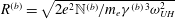 $R^{(b)}=\sqrt{2e^{2}\mathbb{ N}^{(b)}/m_{e}{\it\gamma}^{(b)\,3}{\it\omega}_{UH}^{2}}$
and have substituted it into (6.23).
$R^{(b)}=\sqrt{2e^{2}\mathbb{ N}^{(b)}/m_{e}{\it\gamma}^{(b)\,3}{\it\omega}_{UH}^{2}}$
and have substituted it into (6.23).
In order to consider in more detail the betatron oscillations, it is convenient to introduce dimensionless variables whose units are defined as follows:
 $$\begin{eqnarray}\left.\begin{array}{@{}c@{}}[t]={\it\omega}_{UH}^{-1},\quad [r]=c/{\it\omega}_{UH},\quad [p]=m_{e}c,\quad [\mathbb{N}^{(b)}]=m_{e}c^{2}/2e^{2},\\ \text{}[\mathbb{M}^{(b)}]=m_{e}c^{2}/{\it\omega}_{UH},\quad [n^{(b)}]=n_{0}.\end{array}\right\}\end{eqnarray}$$
In normalized variables (6.14) and (6.15) take the form
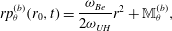 $$\begin{eqnarray}rp_{{\it\theta}}^{(b)}(r_{0},t)=\frac{{\it\omega}_{Be}}{2{\it\omega}_{UH}}r^{2}+\mathbb{M}_{{\it\theta}}^{(b)},\end{eqnarray}$$
and
 $$\begin{eqnarray}\ddot{r}+r=\frac{\mathbb{M}_{{\it\theta}}^{(b)\,2}}{{\it\gamma}^{(b)}r^{3}}+\frac{\mathbb{N}^{(b)}}{{\it\gamma}^{(b)\,3}r},\end{eqnarray}$$
respectively. The functions
 $\mathbb{M}_{{\it\theta}}^{(b)}$
and
$\mathbb{M}_{{\it\theta}}^{(b)}$
and
 $\mathbb{N}^{(b)}$
depend on the Lagrange coordinate
$\mathbb{N}^{(b)}$
depend on the Lagrange coordinate
 $r_{0}$
and on a parameter.
$r_{0}$
and on a parameter.

Figure 16. Projections of two electron trajectories on the transverse
 $(y,z)$
plane for (a) the case of radial oscillations and relatively fast rotation with
$(y,z)$
plane for (a) the case of radial oscillations and relatively fast rotation with
 $r_{0}=1$
,
$r_{0}=1$
,
 $\mathbb{M}_{{\it\theta}}^{(b)}=1$
,
$\mathbb{M}_{{\it\theta}}^{(b)}=1$
,
 $\mathbb{N}^{(b)}=10$
,
$\mathbb{N}^{(b)}=10$
,
 ${\it\gamma}^{(b)}=5$
,
${\it\gamma}^{(b)}=5$
,
 ${\it\omega}_{Be}/{\it\omega}_{UH}=1/2$
,
${\it\omega}_{Be}/{\it\omega}_{UH}=1/2$
,
 $r_{0}=1$
and (b) the case of radial oscillations and relatively slow rotation with
$r_{0}=1$
and (b) the case of radial oscillations and relatively slow rotation with
 $r_{0}=1$
,
$r_{0}=1$
,
 $\mathbb{M}_{{\it\theta}}^{(b)}=0.01$
,
$\mathbb{M}_{{\it\theta}}^{(b)}=0.01$
,
 $\mathbb{N}^{(b)}=50$
,
$\mathbb{N}^{(b)}=50$
,
 ${\it\gamma}^{(b)}=5$
,
${\it\gamma}^{(b)}=5$
,
 ${\it\omega}_{Be}/{\it\omega}_{UH}=0.05$
.
${\it\omega}_{Be}/{\it\omega}_{UH}=0.05$
.
In figure 16 we show the projections of two electron trajectories on the transverse
 $(y,z)$
plane obtained with numerical integration of (6.25) and (6.26). The angle coordinate
$(y,z)$
plane obtained with numerical integration of (6.25) and (6.26). The angle coordinate
 ${\it\theta}$
obeys the equation
${\it\theta}$
obeys the equation
 $$\begin{eqnarray}r\dot{{\it\theta}}=\frac{p_{{\it\theta}}}{{\it\gamma}^{(b)}}.\end{eqnarray}$$
The parameters corresponding to figure 16(a,b) are as follows. In the frame (a) the Lagrange coordinate equals
 $r_{0}=1$
, the angular momentum and charge inside the radius
$r_{0}=1$
, the angular momentum and charge inside the radius
 $r_{0}$
are
$r_{0}$
are
 $\mathbb{M}_{{\it\theta}}^{(b)}=1$
and
$\mathbb{M}_{{\it\theta}}^{(b)}=1$
and
 $\mathbb{N}^{(b)}=10$
, respectively, the bunch gamma factor is
$\mathbb{N}^{(b)}=10$
, respectively, the bunch gamma factor is
 ${\it\gamma}^{(b)}=5$
, and the ratio
${\it\gamma}^{(b)}=5$
, and the ratio
 ${\it\omega}_{Be}/{\it\omega}_{UH}$
is equal to
${\it\omega}_{Be}/{\it\omega}_{UH}$
is equal to
 $1/2$
. The trajectory in figure 16(b) is obtained for
$1/2$
. The trajectory in figure 16(b) is obtained for
 $r_{0}=1$
,
$r_{0}=1$
,
 $\mathbb{M}_{{\it\theta}}^{(b)}=0.01$
,
$\mathbb{M}_{{\it\theta}}^{(b)}=0.01$
,
 $\mathbb{N}^{(b)}=50$
,
$\mathbb{N}^{(b)}=50$
,
 ${\it\gamma}^{(b)}=5$
,
${\it\gamma}^{(b)}=5$
,
 ${\it\omega}_{Be}/{\it\omega}_{UH}=0.05$
. As we see, the trajectories are confined within the ring limited by
${\it\omega}_{Be}/{\it\omega}_{UH}=0.05$
. As we see, the trajectories are confined within the ring limited by
 $r_{max}$
and
$r_{max}$
and
 $r_{min}$
determined by the energy integral (6.22). The element of the electron fluid oscillates in the radial direction between
$r_{min}$
determined by the energy integral (6.22). The element of the electron fluid oscillates in the radial direction between
 $r_{max}$
and
$r_{max}$
and
 $r_{min}$
and rotates. In the case shown in figure 16(a) the angular momentum and the magnetic field, i.e. the Larmor frequency
$r_{min}$
and rotates. In the case shown in figure 16(a) the angular momentum and the magnetic field, i.e. the Larmor frequency
 ${\it\omega}_{Be}$
, are relatively large. The trajectory in figure 16(b) shows relatively slow rotation.
${\it\omega}_{Be}$
, are relatively large. The trajectory in figure 16(b) shows relatively slow rotation.
6.4 Constraint on the number of particles in the bunch
At the equilibrium the bunch density is given by expression (6.21). As can be seen, in the case when the bunch rotation effects are negligibly weak, the equilibrium bunch density
 $n^{(b)}=n_{0}{\it\gamma}^{b\,2}$
is a factor
$n^{(b)}=n_{0}{\it\gamma}^{b\,2}$
is a factor
 ${\it\gamma}^{b\,2}$
larger than the density of the ions inside the cavity. By comparing the electric field produced by the electron bunch (6.10) at the distance of the order of the cavity radius
${\it\gamma}^{b\,2}$
larger than the density of the ions inside the cavity. By comparing the electric field produced by the electron bunch (6.10) at the distance of the order of the cavity radius
 $r_{c}$
with the electric field in the cavity
$r_{c}$
with the electric field in the cavity
 $2{\rm\pi}n_{0}er_{c}$
we find the constraint on the number of particles per unit length in the bunch to be below the overloading limit:
$2{\rm\pi}n_{0}er_{c}$
we find the constraint on the number of particles per unit length in the bunch to be below the overloading limit:
 $$\begin{eqnarray}N^{(b)}<2{\rm\pi}n_{0}r_{c}^{2}.\end{eqnarray}$$
Thus the total number of electrons in the bunch should be less than
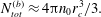 $$\begin{eqnarray}N_{tot}^{(b)}\approx 4{\rm\pi}n_{0}r_{c}^{3}/3.\end{eqnarray}$$
From this equation it follows that
 $N_{tot}^{(b)}\propto n_{0}^{-1/2}$
, i.e. the lower the plasma density the higher the accelerated electron number can be. Using the relationship between the driver laser power, the laser amplitude and the plasma density given by (4.1) we can express the overloading threshold as
$N_{tot}^{(b)}\propto n_{0}^{-1/2}$
, i.e. the lower the plasma density the higher the accelerated electron number can be. Using the relationship between the driver laser power, the laser amplitude and the plasma density given by (4.1) we can express the overloading threshold as
 $$\begin{eqnarray}N_{tot}^{(b)}\approx \frac{{\it\lambda}}{6{\rm\pi}r_{e}}\sqrt{\frac{{\mathcal{P}}}{\bar{{\mathcal{P}}}}},\end{eqnarray}$$
where
 $r_{e}=e^{2}/m_{e}c^{2}=2.8\times 10^{-13}$
cm is the classical electron radius. For a
$r_{e}=e^{2}/m_{e}c^{2}=2.8\times 10^{-13}$
cm is the classical electron radius. For a
 $1~{\rm\mu}\text{m}$
laser wavelength the ratio
$1~{\rm\mu}\text{m}$
laser wavelength the ratio
 ${\it\lambda}/6{\rm\pi}r_{e}$
is equal to
${\it\lambda}/6{\rm\pi}r_{e}$
is equal to
 $1.8\times 10^{7}$
. If the laser power equals 1 PW this yields
$1.8\times 10^{7}$
. If the laser power equals 1 PW this yields
 $N_{tot}^{(b)}\approx 4.3\times 10^{9}$
, which is equivalent to the electric charge of 800 pC.
$N_{tot}^{(b)}\approx 4.3\times 10^{9}$
, which is equivalent to the electric charge of 800 pC.
7 Multi-stage configurations
A multi-stage LWFA accelerator consists of several succeeding accelerating stages inside of which the wake waves are generated by a single or by multiple laser pulses. The electron injection can be provided either in the nonlinear wake wave breaking in homogeneous (Bulanov et al. Reference Bulanov, Inovenkov, Kirsanov, Naumova and Sakharov1992; Modena et al. Reference Modena, Najmudin, Dangor, Clayton, Marsh, Joshi, Malka, Darrow, Danson and Neely1995; Bulanov et al. Reference Bulanov, Pegoraro, Pukhov and Sakharov1997a ; Pukhov & Meyer-ter Vehn Reference Pukhov and Meyer-ter Vehn2002) or inhomogeneous plasmas (Bulanov et al. Reference Bulanov, Naumova, Pegoraro and Sakai1998; Suk et al. Reference Suk, Barov, Rosenzweig and Esarey2001; Thompson et al. Reference Thompson, Rosenzweig and Suk2004; Tomassini et al. Reference Tomassini, Galimberti, Giulietti, Giulietti, Gizzi, Labate and Pegoraro2004; Brantov et al. Reference Brantov, Kando, Kotaki, Yu and Bulanov2008), or by optical injection (Esarey et al. Reference Esarey, Hubbard, Leemans, Ting and Sprangle1997; Kotaki et al. Reference Kotaki, Masuda, Kando, Koga and Nakajima2004; Faure et al. Reference Faure, Rechatin, Norlin, Lifschitz, Glinec and Malka2006; Kotaki et al. Reference Kotaki, Daito, Kando, Hayashi, Kawase, Kameshima, Fukuda, Homma, Ma and Chen2009), by ionization injection (Schroeder et al. Reference Schroeder, Benedetti, Bulanov, Chen, Esarey, Geddes, Vay, Yu and Leemans2015) mechanisms and from the clusters (Fukuda et al. Reference Fukuda, Akahane, Aoyama, Hayashi, Homma, Inoue, Kando, Kanazawa, Kiriyama and Kondo2007).
The second and subsequent stages can be used for enhancing the energy of the accelerated electron bunch and for improving its quality. Enhancing the bunch quality in a two stage LWFA accelerator has been demonstrated in experiments (Pollock et al. Reference Pollock, Clayton, Ralph, Albert, Davidson, Divol, Filip, Glenzer, Herpoldt and Lu2011; Otsuka et al. Reference Otsuka, Nakmura, Nakanii, Masuda, Sueda, Pathak, Iwasa, Takeguchi, Osako and Zhidkov2015). An electron bunch being accelerated in the previous (injector) stage has the length determined by the process of the wake wave breaking and by the length of the wake wavelength. In the subsequent stage, if the plasma density there is substantially lower than in the injector stage, it appears to have a length significantly shorter than the wake wave wavelength. Under these conditions the bunch rotation in the phase space can lead to the electron energy narrowing provided the bunch leaves the stage being at the top of the separatrix. Thus the subsequent stage operates as an accelerator and phase rotator (Otsuka et al. Reference Otsuka, Nakmura, Nakanii, Masuda, Sueda, Pathak, Iwasa, Takeguchi, Osako and Zhidkov2015). The phase rotator has been demonstrated to improve the quality of laser accelerated ion beams (Noda et al. Reference Noda, Nakamura, Iwashita, Sakabe, Hashida, Shirai, Shimizu, Tongu, Ito and Souda2006; Nakamura et al. Reference Nakamura, Ikegami, Iwashita, Shirai, Tongu, Souda, Daido, Mori, Kado and Sagisaka2007).
7.1 Injector
Assuming the wake wave breaking mechanism of the electron injection we shall consider the first stage(s) of the multi-stage accelerator as the injector. The condition of the wake wave breaking corresponds to the case when the wake field given by (2.26) exceeds the wave breaking threshold (2.16). In the limit
 ${\it\gamma}_{w}\gg 1$
this condition yields a relationship between the amplitude of the driver laser pulse and
${\it\gamma}_{w}\gg 1$
this condition yields a relationship between the amplitude of the driver laser pulse and
 ${\it\gamma}_{w}$
:
${\it\gamma}_{w}$
:
 $$\begin{eqnarray}1+a^{2}\geqslant {\it\gamma}_{w},\end{eqnarray}$$
which is equivalent to the condition
 $a^{3/2}\geqslant ({\it\omega}/{\it\omega}_{pe})$
. Using the relationship between the driver laser power, the laser amplitude and the plasma density given by (4.1) we can write the wake wave breaking condition in the form
$a^{3/2}\geqslant ({\it\omega}/{\it\omega}_{pe})$
. Using the relationship between the driver laser power, the laser amplitude and the plasma density given by (4.1) we can write the wake wave breaking condition in the form
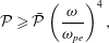 $$\begin{eqnarray}{\mathcal{P}}\geqslant \bar{{\mathcal{P}}}\left(\frac{{\it\omega}}{{\it\omega}_{pe}}\right)^{4},\end{eqnarray}$$
which is well above the threshold of the relativistic self-focusing (Litvak Reference Litvak1970; Sun et al.
Reference Sun, Ott, Lee and Guzdar1987). The driver length optimal for wake wave generation, (2.21)–(2.23), in the limit
 $a\approx 1$
for driver power at the wave breaking threshold (7.2), equals
$a\approx 1$
for driver power at the wave breaking threshold (7.2), equals
 $$\begin{eqnarray}l_{opt}\approx \frac{{\rm\pi}c}{{\it\omega}_{pe}}.\end{eqnarray}$$
This results in the requirement on the laser pulse energy
 ${\mathcal{E}}_{las}={\mathcal{P}}l_{opt}/c$
:
${\mathcal{E}}_{las}={\mathcal{P}}l_{opt}/c$
:
 $$\begin{eqnarray}{\mathcal{E}}_{las}=\bar{{\mathcal{E}}}\left(\frac{{\it\omega}}{{\it\omega}_{pe}}\right)^{3},\end{eqnarray}$$
where
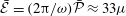 $\bar{{\mathcal{E}}}=(2{\rm\pi}/{\it\omega})\bar{{\mathcal{P}}}\approx 33{\it\mu}$
J. From (7.2) and (7.4) follows that the energy of the laser injector can also be expressed in terms of the laser power:
$\bar{{\mathcal{E}}}=(2{\rm\pi}/{\it\omega})\bar{{\mathcal{P}}}\approx 33{\it\mu}$
J. From (7.2) and (7.4) follows that the energy of the laser injector can also be expressed in terms of the laser power:
 $$\begin{eqnarray}{\mathcal{E}}_{las}=\bar{{\mathcal{E}}}\left(\frac{{\mathcal{P}}}{\bar{{\mathcal{P}}}}\right)^{3/2}.\end{eqnarray}$$
For example, the energy of a 2 PW laser injector should be of the order of 30 J, and the energy of a 200 TW laser is approximately 30 times lower.
As we see, the 1-D approximation implies too high requirements for the laser pulse power and energy. These requirements can be mitigated in the 3-D regime when the laser pulse undergoing the relativistic self-focusing forms a cavity (bubble) in an underdense plasma (Pukhov & Meyer-ter Vehn Reference Pukhov and Meyer-ter Vehn2002). Inside the cavity the wake wave breaking develops in the transverse wave breaking regime described in Bulanov et al. (Reference Bulanov, Pegoraro, Pukhov and Sakharov1997a
), Bulanov et al. (Reference Bulanov, Califano, Dudnikova, Vshivkov, Liseikina, Naumova, Pegoraro, Sakai and Sakharov1999a
), Liseikina et al. (Reference Liseikina, Califano, Vshivkov, Pegoraro and Bulanov1999), Kando et al. (Reference Kando, Fukuda, Kotaki, Koga, Bulanov, Tajima, Chao, Pitthan, Schuler and Zhidkov2007), Corde et al. (Reference Corde, Thaury, Lifschitz, Lambert, Ta Phuoc, Davoine, Lehe, Douillet, Rousse and Malka2013), Islam et al. (Reference Islam, Brunetti, Shanks, Ersfeld, Issac, Cipiccia, Anania, Welsh, Wiggins and Noble2015). The electron energy
 ${\approx}m_{e}c^{2}a$
is of the order of or above the injection threshold given by (3.12) for
${\approx}m_{e}c^{2}a$
is of the order of or above the injection threshold given by (3.12) for
 ${\it\varphi}_{m}\approx m_{e}c^{2}a/e$
.
${\it\varphi}_{m}\approx m_{e}c^{2}a/e$
.
In a plasma with inhomogeneous density, the phase-mixing phenomenon leads to the wake wave breaking with the electron injection even for an initial electron energy determined by the wake wave amplitude well below the injection threshold in homogeneous plasmas (Bulanov et al. Reference Bulanov, Naumova, Pegoraro and Sakai1998; Brantov et al. Reference Brantov, Kando, Kotaki, Yu and Bulanov2008; Geddes et al. Reference Geddes, Nakamura, Plateau, Toth, Cormier-Michel, Esarey, Schroeder, Cary and Leemans2008). However, in the limit of substantially low wave amplitude, this regime requires a good enough quality wake wave to be formed and it may result in electron injection into a bucket located far behind the laser pulse driver.

Figure 17. Multi-even stage accelerator comprising the injector and equal stages. (a) Schematic of the multi-equal stage LWFA accelerator. (b) Phase plots
 $(X,{\it\gamma})$
corresponding to the
$(X,{\it\gamma})$
corresponding to the
 $j-1$
th,
$j-1$
th,
 $j$
th, and
$j$
th, and
 $j+1$
th stages of the accelerator.
$j+1$
th stages of the accelerator.
7.2 Multi-equal stage configuration
In the case of a multi-stage configuration with equal stages the energy gain in each subsequent stage is given by (3.22), i.e.
 $$\begin{eqnarray}{\rm\Delta}{\it\gamma}=\frac{a^{4}+2a^{2}}{(1-{\it\beta}_{w})(1+a^{2})},\end{eqnarray}$$
provided the electron has been injected at the local minimum of the electrostatic potential as illustrated in figure 17. Having interacted with
 $J$
stages, the electron injected in the injector with energy
$J$
stages, the electron injected in the injector with energy
 ${\it\gamma}_{inj}={\it\gamma}_{w}$
achieves a final energy equal to
${\it\gamma}_{inj}={\it\gamma}_{w}$
achieves a final energy equal to
 $$\begin{eqnarray}{\it\gamma}_{J}={\it\gamma}_{w}+\frac{J(a^{4}+2a^{2})}{(1-{\it\beta}_{w})(1+a^{2})}\end{eqnarray}$$
As seen, for
 $a\approx 1$
, the final energy is of the order of
$a\approx 1$
, the final energy is of the order of
 ${\it\gamma}_{J}\approx 3J{\it\gamma}_{w}^{2}$
. The length of one stage is equal to the dephasing length,
${\it\gamma}_{J}\approx 3J{\it\gamma}_{w}^{2}$
. The length of one stage is equal to the dephasing length,
 $l_{acc}$
, given by (3.2):
$l_{acc}$
, given by (3.2):
 $l_{acc}={\it\lambda}{\it\gamma}_{w}^{3}$
. Thus the total length of the multi-stage accelerator with equal length stages is
$l_{acc}={\it\lambda}{\it\gamma}_{w}^{3}$
. Thus the total length of the multi-stage accelerator with equal length stages is
 $$\begin{eqnarray}L_{acc}=J{\it\lambda}{\it\gamma}_{w}^{3}={\it\lambda}({\it\gamma}_{J}/3)^{3/2}J^{-1/2},\end{eqnarray}$$
i.e. for fixed final energy of the accelerated electrons,
 ${\it\gamma}_{J}$
, the acceleration length is shorter for a larger number of stages
${\it\gamma}_{J}$
, the acceleration length is shorter for a larger number of stages
 $J$
. Apparently, the number of the stages cannot be arbitrarily large, because the length of one stage cannot be smaller than
$J$
. Apparently, the number of the stages cannot be arbitrarily large, because the length of one stage cannot be smaller than
 $l_{st}={\it\lambda}(l_{las}/{\rm\pi}{\it\lambda})^{3}$
under the conditions requiring the laser pulse length to be optimal for the wake wave excitation.
$l_{st}={\it\lambda}(l_{las}/{\rm\pi}{\it\lambda})^{3}$
under the conditions requiring the laser pulse length to be optimal for the wake wave excitation.
An additional constraint on the number of the stages
 $J$
stems from the matching requirement between the electron bunch accelerated in the
$J$
stems from the matching requirement between the electron bunch accelerated in the
 $(j-1)$
th stage with the wake field in the
$(j-1)$
th stage with the wake field in the
 $(j)$
th stage. Under more or less realistic conditions, when the matching is not ideal, the unavoidable deterioration of the electron beam quality (e.g. see Cheshkov et al.
Reference Cheshkov, Tajima, Horton and Yokoya2000; Chiu et al.
Reference Chiu, Cheshkov and Tajima2000; Deng et al.
Reference Deng, Liu, Nakajima, Xia, Wang, Li, Lu, Zhang, Ju and Tian2012) may become unacceptably high for a large enough number of stages.
$(j)$
th stage. Under more or less realistic conditions, when the matching is not ideal, the unavoidable deterioration of the electron beam quality (e.g. see Cheshkov et al.
Reference Cheshkov, Tajima, Horton and Yokoya2000; Chiu et al.
Reference Chiu, Cheshkov and Tajima2000; Deng et al.
Reference Deng, Liu, Nakajima, Xia, Wang, Li, Lu, Zhang, Ju and Tian2012) may become unacceptably high for a large enough number of stages.
7.3 Multi-uneven stage configuration
The number of the stages can be made smaller in a multi-uneven stage LWFA accelerator, whose schematic view is presented in figure 18. In this configuration, the plasma density in the succeeding stage is lower than the plasma density in the preceding stage, and the length of the succeeding stage is larger than that of the preceding.

Figure 18. Multi-uneven stage accelerator comprising the injector and unequal stages. (a) Scematic of the multi-unequal stage LWFA accelerator. (b) Phase plots
 $(X,{\it\gamma})$
corresponding to the
$(X,{\it\gamma})$
corresponding to the
 $j-1$
th,
$j-1$
th,
 $j$
th and
$j$
th and
 $j+1$
th stages of the accelerator.
$j+1$
th stages of the accelerator.
The energy gained by the electrons accelerated in the preceding stage
 ${\it\gamma}_{j-1}\approx {\it\gamma}_{w,j-1}^{2}$
(here we assume that the laser driver pulse normalized amplitude is of the order of unity,
${\it\gamma}_{j-1}\approx {\it\gamma}_{w,j-1}^{2}$
(here we assume that the laser driver pulse normalized amplitude is of the order of unity,
 $a_{j-1}=1$
) is equal to the injection energy for the succeeding stage, i.e.
$a_{j-1}=1$
) is equal to the injection energy for the succeeding stage, i.e.
 $$\begin{eqnarray}{\it\gamma}_{w,j-1}^{2}={\it\gamma}_{w,j}.\end{eqnarray}$$
It is assumed that the electrons enter the wake field in succeeding stages in the phase corresponding to the singular point,
 $X$
-point, on the separatrix as shown in figure 14(b). We note a similarity between this process and the ‘rephasing’ considered by Döpp et al. (Reference Döpp, Guillaume, Thaury, Lifschitz, Phuoc and Malka2015), Guillaume et al. (Reference Guillaume, Döpp, Thaury, Ta Phuoc, Lifschitz, Grittani, Goddet, Tafzi, Chou and Veisz2015b
). The equation (7.9) gives a relationship between the parameters of the
$X$
-point, on the separatrix as shown in figure 14(b). We note a similarity between this process and the ‘rephasing’ considered by Döpp et al. (Reference Döpp, Guillaume, Thaury, Lifschitz, Phuoc and Malka2015), Guillaume et al. (Reference Guillaume, Döpp, Thaury, Ta Phuoc, Lifschitz, Grittani, Goddet, Tafzi, Chou and Veisz2015b
). The equation (7.9) gives a relationship between the parameters of the
 $(j-1)$
th and
$(j-1)$
th and
 $j$
th stages. From (7.9) it follows that for known plasma density in the first stage,
$j$
th stages. From (7.9) it follows that for known plasma density in the first stage,
 $n_{1}$
, determined by the matching conditions with the injector stage, the density in the
$n_{1}$
, determined by the matching conditions with the injector stage, the density in the
 $j$
th stage is equal to
$j$
th stage is equal to
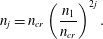 $$\begin{eqnarray}n_{j}=n_{cr}\left(\frac{n_{1}}{n_{cr}}\right)^{2j}.\end{eqnarray}$$
The
 $j$
th stage length depends on the stage number as
$j$
th stage length depends on the stage number as
 $$\begin{eqnarray}l_{j}={\it\lambda}\left(\frac{n_{cr}}{n_{1}}\right)^{3j}={\it\lambda}\left(\frac{l_{1}}{{\it\lambda}}\right)^{3j},\end{eqnarray}$$
where
 $l_{1}={\it\lambda}(n_{cr}/n_{1})^{3}$
is the length of the first stage. The energy of the electrons achieved as a result of interacting with
$l_{1}={\it\lambda}(n_{cr}/n_{1})^{3}$
is the length of the first stage. The energy of the electrons achieved as a result of interacting with
 $J$
stages equals
$J$
stages equals
 $$\begin{eqnarray}\displaystyle {\it\gamma}_{J} & = & \displaystyle \mathop{\sum }_{j=1}^{J}\left(\frac{n_{cr}}{n_{j}}\right)=\mathop{\sum }_{j=1}^{J}\left(\frac{n_{cr}}{n_{1}}\right)^{2j}\nonumber\\ \displaystyle & = & \displaystyle \frac{\left({\displaystyle \frac{n_{cr}}{n_{1}}}\right)^{2J}-1}{1-\left({\displaystyle \frac{n_{1}}{n_{cr}}}\right)^{2}}\approx \left(\frac{n_{cr}}{n_{1}}\right)^{2J}.\end{eqnarray}$$
As we see, the accelerated electron energy grows exponentially with the number of stages in the limit
 $J\rightarrow \infty$
:
$J\rightarrow \infty$
:
 $$\begin{eqnarray}{\it\gamma}_{J}\approx \exp \left(J\ln \frac{n_{cr}}{n_{1}}\right).\end{eqnarray}$$
In the relationships obtained above the electron density inside the first stage has remained undetermined. It can be found from the condition imposed on the required electric charge of the accelerated electron bunch. According to (6.29) we have a relationship between the total number of accelerated electrons and the plasma density. The ratio
 $n_{cr}/n_{1}$
can also be chosen for desired electron energy
$n_{cr}/n_{1}$
can also be chosen for desired electron energy
 ${\it\gamma}_{J}$
and the finite number of the stages,
${\it\gamma}_{J}$
and the finite number of the stages,
 $J$
. The required laser power and energy, given by the relationships obtained above in § 5.1, are determined by the parameters of the last,
$J$
. The required laser power and energy, given by the relationships obtained above in § 5.1, are determined by the parameters of the last,
 $J\text{th}$
stage.
$J\text{th}$
stage.
8 PIC simulations of the injection–acceleration triple-stage configuration
In order to achieve energy spreads and transverse emittances necessary for various applications, e.g. for the table-top free electron X-ray laser, we are considering staged acceleration of LWFA electrons as a possible method. In this scheme three stages are used in the electron beam acceleration: (i) beam injector, (ii) phase rotator and (iii) booster. The use of a multi-stage LWFA configuration has the potential to dramatically improve the quality of the accelerated electron bunch.
8.1 Simulation parameters and set-up
The simulation parameters are chosen so that the LWFA electrons can have energies above 1 GeV, a charge of over 10 pC, be stable, have relative energy spreads between
 $10^{-3}$
and
$10^{-3}$
and
 $10^{-4}$
and have a transverse emittance of less than 0.1 mm mrad.
$10^{-4}$
and have a transverse emittance of less than 0.1 mm mrad.
The beam injector involves using a moderate power laser pulse for the LWFA of electrons generating electron beams with energies of the order of 30 to 40 MeV. These electron beams are then phase space rotated via conventional accelerator components or a laser wake field to reduce their relative energy spread. The phase space rotated electron beams are then again accelerated in a booster using a high power laser via LWFA to 1 GeV. The final electron beam is expected to have sufficiently low energy spread and transverse emittance for injection into an undulator for lasing. Here we examine the (i) beam injector and (ii) phase rotator stages both using LWFA with a moderate power laser pulse.
For control of the beam energy we consider injection via a sharp density gradient (Suk et al. Reference Suk, Barov, Rosenzweig and Esarey2001; Tomassini et al. Reference Tomassini, Galimberti, Giulietti, Giulietti, Gizzi, Labate and Pegoraro2004; Brantov et al. Reference Brantov, Kando, Kotaki, Yu and Bulanov2008). For this study we performed 2-D PIC simulations using the REMP code (Esirkepov Reference Esirkepov2001). We have previously presented PIC simulations in Koga et al. (Reference Koga, Mori, Kotaki, Bulanov, Esirkepov, Kiriyama and Kando2016) using a density gradient to inject electrons. Here, we present simulations where we have further modified the density profile to achieve smaller energy spread.
The simulation box is
 $300{\it\lambda}_{0}$
in the
$300{\it\lambda}_{0}$
in the
 $x$
(laser propagation) direction and
$x$
(laser propagation) direction and
 $240{\it\lambda}_{0}$
in the
$240{\it\lambda}_{0}$
in the
 $y$
direction where the grid size is
$y$
direction where the grid size is
 ${\it\Delta}_{x}={\it\lambda}_{0}/16$
and
${\it\Delta}_{x}={\it\lambda}_{0}/16$
and
 ${\it\Delta}_{y}={\it\lambda}_{0}/8$
. The simulation box moves in the
${\it\Delta}_{y}={\it\lambda}_{0}/8$
. The simulation box moves in the
 $+x$
direction at the speed of light,
$+x$
direction at the speed of light,
 $c$
.
$c$
.
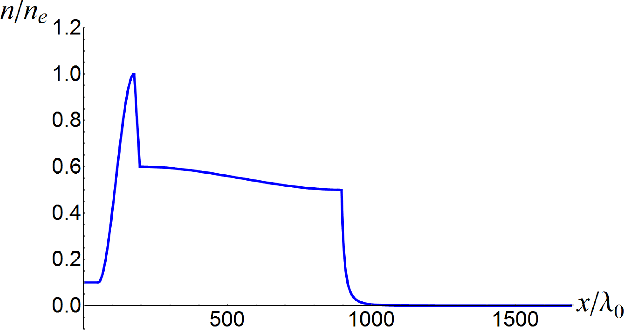
Figure 19. Plasma density profile with a sharp density gradient of width
 $20{\it\lambda}_{0}$
at
$20{\it\lambda}_{0}$
at
 $x=175{\it\lambda}_{0}$
(injector) and a sharp density drop off at
$x=175{\it\lambda}_{0}$
(injector) and a sharp density drop off at
 $x=895{\it\lambda}_{0}$
(end of phase rotation and acceleration) along the laser propagation direction with the laser entering from the left. The density is normalized by the peak plasma density
$x=895{\it\lambda}_{0}$
(end of phase rotation and acceleration) along the laser propagation direction with the laser entering from the left. The density is normalized by the peak plasma density
 $n_{e}$
and the propagation distance is normalized by the laser wavelength
$n_{e}$
and the propagation distance is normalized by the laser wavelength
 ${\it\lambda}_{0}$
.
${\it\lambda}_{0}$
.
Figure 19 shows the density profile for the simulation in the laser propagation direction with the laser pulse entering from the left. The density is normalized by the peak electron density
 $n_{e}$
which corresponds to
$n_{e}$
which corresponds to
 ${\it\omega}_{pe}/{\it\omega}_{0}=0.05$
where
${\it\omega}_{pe}/{\it\omega}_{0}=0.05$
where
 ${\it\omega}_{pe}=\sqrt{4{\rm\pi}e^{2}n_{e}/m_{e}}$
with
${\it\omega}_{pe}=\sqrt{4{\rm\pi}e^{2}n_{e}/m_{e}}$
with
 $e$
being the electron charge,
$e$
being the electron charge,
 $m_{e}$
being the electron mass and
$m_{e}$
being the electron mass and
 ${\it\omega}_{0}$
is the laser frequency. A maximum of 6 macro-particles per cell are used at the peak density. In the direction perpendicular to the laser propagation direction,
${\it\omega}_{0}$
is the laser frequency. A maximum of 6 macro-particles per cell are used at the peak density. In the direction perpendicular to the laser propagation direction,
 $y$
, the density is taken to be uniform. The density profile can be seen to be composed of three stages in the laser propagation direction: (i) injector, (ii) phase rotator and accelerator and (iii) booster.
$y$
, the density is taken to be uniform. The density profile can be seen to be composed of three stages in the laser propagation direction: (i) injector, (ii) phase rotator and accelerator and (iii) booster.
(i) In the propagation direction,
 $x$
, initially a vacuum region up to
$x$
, initially a vacuum region up to
 $x_{1}=50{\it\lambda}_{0}$
exists at which point the density starts at
$x_{1}=50{\it\lambda}_{0}$
exists at which point the density starts at
 $n_{1}=0.1n_{e}$
and then increases to a peak of
$n_{1}=0.1n_{e}$
and then increases to a peak of
 $n_{2}=n_{e}$
at
$n_{2}=n_{e}$
at
 $x_{2}=175{\it\lambda}_{0}$
according to
$x_{2}=175{\it\lambda}_{0}$
according to
 $$\begin{eqnarray}n(x)=n_{1}+(n_{2}-n_{1})\left[3-2\left(\frac{x-x_{1}}{x_{2}-x_{1}}\right)\right]\left(\frac{x-x_{1}}{x_{2}-x_{1}}\right)^{2}.\end{eqnarray}$$
After this peak the density drops off as a linear function to
 $n_{3}=0.6n_{e}$
at
$n_{3}=0.6n_{e}$
at
 $x_{3}=195{\it\lambda}_{0}$
over a distance of
$x_{3}=195{\it\lambda}_{0}$
over a distance of
 ${\rm\Delta}x=20{\it\lambda}_{0}$
. Such a type of sharp density drop off can be produced via the generation of a shock front by inserting a razor blade into the supersonic gas jet exiting from a de Laval nozzle (Schmid et al.
Reference Schmid, Buck, Sears, Mikhailova, Tautz, Herrmann, Geissler, Krausz and Veisz2010).
${\rm\Delta}x=20{\it\lambda}_{0}$
. Such a type of sharp density drop off can be produced via the generation of a shock front by inserting a razor blade into the supersonic gas jet exiting from a de Laval nozzle (Schmid et al.
Reference Schmid, Buck, Sears, Mikhailova, Tautz, Herrmann, Geissler, Krausz and Veisz2010).
(ii) From
 $x_{3}$
to
$x_{3}$
to
 $x_{4}=895{\it\lambda}_{0}$
the density varies as
$x_{4}=895{\it\lambda}_{0}$
the density varies as
 $$\begin{eqnarray}n(x)=n_{3}+(n_{4}-n_{3})\left[3-2\left(\frac{x-x_{3}}{x_{4}-x_{3}}\right)\right]\left(\frac{x-x_{3}}{x_{4}-x_{3}}\right)^{2},\end{eqnarray}$$
where
 $n_{4}=0.5n_{e}$
. In this region the injected electron bunch is expected to be simultaneously accelerated and phase rotated.
$n_{4}=0.5n_{e}$
. In this region the injected electron bunch is expected to be simultaneously accelerated and phase rotated.
(iii) At the end of this region we have the density drop off sharply as a power-law function,
 $$\begin{eqnarray}n(x)=n_{4}\left[\left(\frac{x-x_{4}}{b}\right)+1\right]^{m},\end{eqnarray}$$
where
 $b=30$
and
$b=30$
and
 $m=-3$
until
$m=-3$
until
 $x_{5}=1695{\it\lambda}_{0}$
, after this the density is held constant at
$x_{5}=1695{\it\lambda}_{0}$
, after this the density is held constant at
 $0.001n_{e}$
, which is effectively zero. In this study we leave the investigation of this booster region up to 1 GeV by a second high power laser pulse for future work.
$0.001n_{e}$
, which is effectively zero. In this study we leave the investigation of this booster region up to 1 GeV by a second high power laser pulse for future work.
The reason for the second sharp drop off near the end of the laser propagation is to stop the acceleration of the electrons in the wake field near the point of dephasing where the energy spread is expected to be smallest (see also Geddes et al.
Reference Geddes, Toth, van Tilborg, Esarey, Schroeder, Bruhwiler, Nieter, Cary and Leemans2004). In other words we are phase rotating the electron bunch until the phase space volume is minimized in
 $(x,p_{x})$
space.
$(x,p_{x})$
space.
The laser is injected initially from the left boundary of the simulation box with a pulse length of
 $12.5{\it\lambda}_{0}$
(FWHM – Full Width Half Maximum) and a spot size of
$12.5{\it\lambda}_{0}$
(FWHM – Full Width Half Maximum) and a spot size of
 $12.5{\it\lambda}_{0}$
(FWHM) at the focus point, which is at the beginning of the sharp density drop off at
$12.5{\it\lambda}_{0}$
(FWHM) at the focus point, which is at the beginning of the sharp density drop off at
 $175{\it\lambda}_{0}$
with the assumption of Gaussian focusing. The normalized amplitude,
$175{\it\lambda}_{0}$
with the assumption of Gaussian focusing. The normalized amplitude,
 $a_{0}\equiv eE_{0}/m_{e}{\it\omega}_{0}c$
, where
$a_{0}\equiv eE_{0}/m_{e}{\it\omega}_{0}c$
, where
 $E_{0}$
is the peak field amplitude, is set to be 1.5.
$E_{0}$
is the peak field amplitude, is set to be 1.5.
8.2 Simulation results
Figure 20(a) shows the density of the plasma right after the laser pulse has passed the sharp density gradient at
 $x=175{\it\lambda}_{0}$
with the laser propagating from left to right (injector). The density is normalized by
$x=175{\it\lambda}_{0}$
with the laser propagating from left to right (injector). The density is normalized by
 $n_{e}$
where darker colours refer to higher densities on a logarithmic scale as indicated by the colour bar on the top right. In figure 20(b) one can see where an electron bunch has been injected into the second bucket of the wake wave and is being further accelerated (phase rotation and acceleration). Since the injection point is determined by the depth and length of the sharp density gradient, we have chosen the injection into the second bucket, because we have found that with our investigated parameters the electron bunch is modified by the back of the laser pulse when it is injected into the first bucket (see discussion at the end of § 3.3). Such modifications have been experimentally observed and used as a measurement of the electron bunch duration (Kotaki et al.
Reference Kotaki, Kawase, Hayashi, Mori, Kando, Koga and Bulanov2015).
$n_{e}$
where darker colours refer to higher densities on a logarithmic scale as indicated by the colour bar on the top right. In figure 20(b) one can see where an electron bunch has been injected into the second bucket of the wake wave and is being further accelerated (phase rotation and acceleration). Since the injection point is determined by the depth and length of the sharp density gradient, we have chosen the injection into the second bucket, because we have found that with our investigated parameters the electron bunch is modified by the back of the laser pulse when it is injected into the first bucket (see discussion at the end of § 3.3). Such modifications have been experimentally observed and used as a measurement of the electron bunch duration (Kotaki et al.
Reference Kotaki, Kawase, Hayashi, Mori, Kando, Koga and Bulanov2015).

Figure 20. Density distribution of the plasma electrons (a) at
 $t=230$
in the
$t=230$
in the
 $(x,y)$
plane just after the laser has passed the sharp density gradient at
$(x,y)$
plane just after the laser has passed the sharp density gradient at
 $x=175{\it\lambda}_{0}$
(injector) along the laser propagation direction with the laser entering from the left where the density is normalized by the peak plasma density
$x=175{\it\lambda}_{0}$
(injector) along the laser propagation direction with the laser entering from the left where the density is normalized by the peak plasma density
 $n_{e}$
; (b) at
$n_{e}$
; (b) at
 $t=920$
when the laser propagates in the lower gradually decreasing plasma density region (phase rotation and acceleration); the
$t=920$
when the laser propagates in the lower gradually decreasing plasma density region (phase rotation and acceleration); the
 $x$
and
$x$
and
 $y$
axes are normalized by the laser wavelength
$y$
axes are normalized by the laser wavelength
 ${\it\lambda}_{0}$
and the time,
${\it\lambda}_{0}$
and the time,
 $t$
, is normalized by
$t$
, is normalized by
 $2{\rm\pi}/{\it\omega}_{0}$
.
$2{\rm\pi}/{\it\omega}_{0}$
.
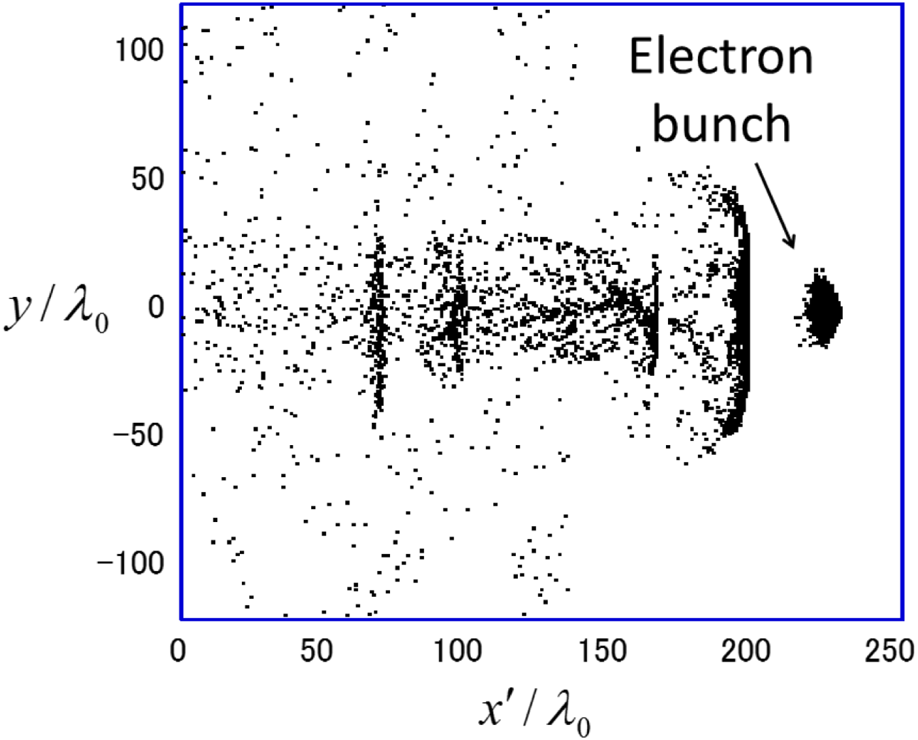
Figure 21. Density distribution of electrons in the plane
 $(x,y)$
after the laser has exited the plasma (practically in vacuum) at
$(x,y)$
after the laser has exited the plasma (practically in vacuum) at
 $t=2000$
which is normalized by
$t=2000$
which is normalized by
 $2{\rm\pi}/{\it\omega}_{0}$
. An electron bunch (indicated by the arrow) can be seen on the right side of the simulation box where the density is normalized by the peak plasma density
$2{\rm\pi}/{\it\omega}_{0}$
. An electron bunch (indicated by the arrow) can be seen on the right side of the simulation box where the density is normalized by the peak plasma density
 $n_{e}$
and the
$n_{e}$
and the
 $x^{\prime }$
and
$x^{\prime }$
and
 $y$
axes are normalized by the laser wavelength
$y$
axes are normalized by the laser wavelength
 ${\it\lambda}_{0}$
. Here
${\it\lambda}_{0}$
. Here
 $x^{\prime }=x-ct$
is the coordinate used in simulation.
$x^{\prime }=x-ct$
is the coordinate used in simulation.
In figure 21 we show the density profile of the electrons after they have exited the plasma at
 $t=2000$
which is normalized by
$t=2000$
which is normalized by
 $2{\rm\pi}/{\it\omega}_{0}$
. The first electron bunch indicated by the arrow in the figure has a maximum spatial duration of
$2{\rm\pi}/{\it\omega}_{0}$
. The first electron bunch indicated by the arrow in the figure has a maximum spatial duration of
 ${\rm\Delta}x\sim 15{\it\lambda}_{0}$
and maximum width of
${\rm\Delta}x\sim 15{\it\lambda}_{0}$
and maximum width of
 ${\rm\Delta}y\sim 30{\it\lambda}_{0}$
.
${\rm\Delta}y\sim 30{\it\lambda}_{0}$
.
Figure 22(a,b) show the electron phase space
 $(x,p_{x})$
and energy,
$(x,p_{x})$
and energy,
 ${\mathcal{E}}_{e}$
, distribution, respectively, at the same time as figure 21. From the phase space plot we see that the electron bunch has a spread in longitudinal momentum of
${\mathcal{E}}_{e}$
, distribution, respectively, at the same time as figure 21. From the phase space plot we see that the electron bunch has a spread in longitudinal momentum of
 ${\rm\Delta}p_{x}\sim 35m_{e}c$
. From the energy distribution it can be seen that the bunch is quasi-monoenergetic with a peak at around 25 MeV. The maximum electron energy is 27.41 MeV as indicated in the figure.
${\rm\Delta}p_{x}\sim 35m_{e}c$
. From the energy distribution it can be seen that the bunch is quasi-monoenergetic with a peak at around 25 MeV. The maximum electron energy is 27.41 MeV as indicated in the figure.

Figure 22. (a) Electron phase space
 $(x^{\prime },p_{x})$
and (b) energy spectrum at
$(x^{\prime },p_{x})$
and (b) energy spectrum at
 $t=2000$
; the
$t=2000$
; the
 $x^{\prime }$
axis is normalized by the laser wavelength
$x^{\prime }$
axis is normalized by the laser wavelength
 ${\it\lambda}_{0}$
which is expressed in terms of the simulation box coordinates,
${\it\lambda}_{0}$
which is expressed in terms of the simulation box coordinates,
 $x^{\prime }=x-ct$
, and the momentum
$x^{\prime }=x-ct$
, and the momentum
 $p_{x}$
is normalized by
$p_{x}$
is normalized by
 $m_{e}c$
.
$m_{e}c$
.

Figure 23. (a) Electron spectrum and (b) electron bunch profile of the first bunch in figure 21; the
 $x^{\prime }$
axis is normalized by the laser wavelength
$x^{\prime }$
axis is normalized by the laser wavelength
 ${\it\lambda}_{0}$
, which is expressed in terms of the simulation box coordinates,
${\it\lambda}_{0}$
, which is expressed in terms of the simulation box coordinates,
 $x^{\prime }=x-ct$
.
$x^{\prime }=x-ct$
.
Figure 23(a,b) show the electron bunch energy spectrum and distribution of the first electron bunch (
 $x^{\prime }/{\it\lambda}_{0}>210$
) along the
$x^{\prime }/{\it\lambda}_{0}>210$
) along the
 $x^{\prime }$
-axis, which is expressed in terms of the simulation box coordinates,
$x^{\prime }$
-axis, which is expressed in terms of the simulation box coordinates,
 $x^{\prime }=x-ct$
, where
$x^{\prime }=x-ct$
, where
 $t$
is the same time as figure 21. The average electron energy is
$t$
is the same time as figure 21. The average electron energy is
 $\langle {\mathcal{E}}_{e}\rangle =24.6$
MeV and the spectrum width has a standard deviation of
$\langle {\mathcal{E}}_{e}\rangle =24.6$
MeV and the spectrum width has a standard deviation of
 ${\it\sigma}=1.46$
MeV resulting in a relative energy spread of approximately
${\it\sigma}=1.46$
MeV resulting in a relative energy spread of approximately
 ${\it\sigma}/\langle {\mathcal{E}}_{e}\rangle \approx 6\,\%$
. Further reduction is possible by rotation in phase space due to some local linear dependence of the energy on spatial coordinate.
${\it\sigma}/\langle {\mathcal{E}}_{e}\rangle \approx 6\,\%$
. Further reduction is possible by rotation in phase space due to some local linear dependence of the energy on spatial coordinate.
The spatial width of the electron bunch has a standard deviation of
 ${\approx}1.94{\it\lambda}_{0}$
. The electron bunch electric charge is equal to
${\approx}1.94{\it\lambda}_{0}$
. The electron bunch electric charge is equal to
 ${\approx}2.45$
pC. In the next phase of our research we will examine the further acceleration of this bunch by a high power laser (booster).
${\approx}2.45$
pC. In the next phase of our research we will examine the further acceleration of this bunch by a high power laser (booster).
These electron bunch parameters are sufficient for further acceleration by proper matching with subsequent stages up to the energy required for various applications including table-top free electron lasers.
We notice here that for achieving the optimal acceleration regime the matching between the injection and acceleration stages should be respected. In other words, the electron energy of the electrons at the exit of the injection stage should be equal to the injection energy of the acceleration phase according to a recipe formulated in § 3.1 (see (3.9)) and in § 7.3, i.e.
 ${\it\gamma}_{inj}={\it\gamma}_{w}$
.
${\it\gamma}_{inj}={\it\gamma}_{w}$
.
9 Conclusion
In this work we have presented a compendium of useful formulas giving relations between the laser and underdense plasma target parameters allowing for obtaining basic dependences of the wake field on the parameters, e.g. the energy scaling of the electrons accelerated by the wake field excited in inhomogeneous media including the multi-equal stage and multi-unequal stage LWFA configurations. The obtained analytical expression for the optimal length of the laser pulse driver can be used for choosing the experiment/simulation parameters in the limit of nonlinear laser–plasma interaction. Using the conditions of the electron trapping to the wake-field acceleration phase we have discussed two scenarios of electron injection with gradual and abrupt density downramp. The analysis of the electron trapping and acceleration allowed us to describe basic properties of the energy spectrum of accelerated particles. The effects of using the chirped laser pulse driver for exciting the wake wave has also been considered. We have found the parameters of the chirped pulse where the chirp can enhance the amplitude of the wake field. We have extended an analysis of the electron beam loading into the accelerating phase taking into account the effects of 3-D geometry of the cavity formed in a plasma behind the ultra-short laser pulse as well as the effects of the longitudinal magnetic field. It has been revealed that the space charge effects change the frequency of the collective betatron oscillations of the electron bunch inside the cavity. The 3-D geometry of the laser pulse and of the guiding structure has been also taken into account in finding regimes of the unlimited LWFA acceleration in inhomogeneous plasmas, in the high laser amplitude limit and in the limit of ultra-short pulse laser with the pulse length substantially less than the optimal length. We have presented the scaling of the LWFA electron acceleration in the multi-even stage and multi-uneven stage configurations. In the first configuration the energy of fast electrons is a linear function of the number of stages. In the second case, the accelerated electron energy grows exponentially with the number of stages. The results of 2-D PIC simulations presented here show the high quality electron acceleration in the triple-stage configuration.
Acknowledgements
This work was funded by ImPACT Program of Council for Science, Technology and Innovation (Cabinet Office, Government of Japan). T.Zh.E. acknowledges the support from JSPS (grant no. 25390135).


