


1 Introduction
Let
 $(W,S)$
be a finite Coxeter group. Kazhdan and Lusztig introduced
$(W,S)$
be a finite Coxeter group. Kazhdan and Lusztig introduced
 $W$
-graphs in [Reference Kazhdan and Lusztig7] in an attempt to capture certain combinatorial features of Kazhdan–Lusztig-cells and of the cell representations associated to them. By definition, every cell representation is a
$W$
-graphs in [Reference Kazhdan and Lusztig7] in an attempt to capture certain combinatorial features of Kazhdan–Lusztig-cells and of the cell representations associated to them. By definition, every cell representation is a
 $W$
-graph representation. The converse is not true.
$W$
-graph representation. The converse is not true.
Gyoja proved that every irreducible representation (and hence every reducible representation as well) of the Hecke algebra
 $H(W,S)$
can be realized as a
$H(W,S)$
can be realized as a
 $W$
-graph representation if
$W$
-graph representation if
 $W$
is finite (see [Reference Gyoja4, 2.3.(1)]). In that proof, the Iwahori–Hecke algebra is embedded into a larger algebra, which I denote
$W$
is finite (see [Reference Gyoja4, 2.3.(1)]). In that proof, the Iwahori–Hecke algebra is embedded into a larger algebra, which I denote
 $\unicode[STIX]{x1D6FA}$
in this paper, and it is proven that there exists a left inverse of this embedding. The
$\unicode[STIX]{x1D6FA}$
in this paper, and it is proven that there exists a left inverse of this embedding. The
 $W$
-graph algebra
$W$
-graph algebra
 $\unicode[STIX]{x1D6FA}$
is constructed in such a way that its modules correspond to
$\unicode[STIX]{x1D6FA}$
is constructed in such a way that its modules correspond to
 $W$
-graphs (up to choice of an appropriate basis). Using any one of these left inverses, every
$W$
-graphs (up to choice of an appropriate basis). Using any one of these left inverses, every
 $H$
-module can be considered as an
$H$
-module can be considered as an
 $\unicode[STIX]{x1D6FA}$
-module, and the result follows.
$\unicode[STIX]{x1D6FA}$
-module, and the result follows.
Gyoja’s proof is nonconstructive, as it does not provide a concrete left inverse of the embedding
 $H{\hookrightarrow}\unicode[STIX]{x1D6FA}$
and does not offer additional information about the
$H{\hookrightarrow}\unicode[STIX]{x1D6FA}$
and does not offer additional information about the
 $W$
-graphs that were constructed in this fashion or any information about general
$W$
-graphs that were constructed in this fashion or any information about general
 $W$
-graphs. In my thesis [Reference Hahn5], I discovered that a careful analysis of
$W$
-graphs. In my thesis [Reference Hahn5], I discovered that a careful analysis of
 $\unicode[STIX]{x1D6FA}$
reveals a fine structure that gives much more detailed information about
$\unicode[STIX]{x1D6FA}$
reveals a fine structure that gives much more detailed information about
 $W$
-graphs. An explicit left inverse utilizing Lusztig’s asymptotic algebra is also provided in [Reference Hahn5, Satz 4.3.2].
$W$
-graphs. An explicit left inverse utilizing Lusztig’s asymptotic algebra is also provided in [Reference Hahn5, Satz 4.3.2].
The starting point for this analysis is the observation that
 $\unicode[STIX]{x1D6FA}$
is a quotient of a path algebra over a quiver which is describable entirely in terms of the Dynkin diagram, a fact that is implicitly contained in Gyoja’s paper but was not interpreted in that way. Gyoja’s definition [Reference Gyoja4, 2.5] gives elements of
$\unicode[STIX]{x1D6FA}$
is a quotient of a path algebra over a quiver which is describable entirely in terms of the Dynkin diagram, a fact that is implicitly contained in Gyoja’s paper but was not interpreted in that way. Gyoja’s definition [Reference Gyoja4, 2.5] gives elements of
 $\unicode[STIX]{x1D6FA}$
that basically realize the vertex idempotents and the edge elements of a path algebra. (This is made precise in Lemma 7.) The first main result of my paper is to give an explicit set of relations for this quotient (Theorem 13). The relations are inspired by the work of Stembridge [Reference Stembridge8], where similar equations appear for the edge weights of so-called admissible
$\unicode[STIX]{x1D6FA}$
that basically realize the vertex idempotents and the edge elements of a path algebra. (This is made precise in Lemma 7.) The first main result of my paper is to give an explicit set of relations for this quotient (Theorem 13). The relations are inspired by the work of Stembridge [Reference Stembridge8], where similar equations appear for the edge weights of so-called admissible
 $W$
-graphs, although they were neither formulated for general
$W$
-graphs, although they were neither formulated for general
 $W$
-graphs nor interpreted as relations for an underlying algebra. This set of relations seems to be different from the presentation Gyoja gives in the appendix of his paper.
$W$
-graphs nor interpreted as relations for an underlying algebra. This set of relations seems to be different from the presentation Gyoja gives in the appendix of his paper.
Once this new presentation of
 $\unicode[STIX]{x1D6FA}$
is established, it is applied to breaking down the structure of
$\unicode[STIX]{x1D6FA}$
is established, it is applied to breaking down the structure of
 $\unicode[STIX]{x1D6FA}$
further. At the moment, this is only done for some small Coxeter groups by a case-by-case analysis, but the proofs are so similar in spirit that I proposed a general conjecture in my thesis whose essence is that
$\unicode[STIX]{x1D6FA}$
further. At the moment, this is only done for some small Coxeter groups by a case-by-case analysis, but the proofs are so similar in spirit that I proposed a general conjecture in my thesis whose essence is that
 $\unicode[STIX]{x1D6FA}$
should also be a quotient of a generalized path algebra over a different quiver which should have
$\unicode[STIX]{x1D6FA}$
should also be a quotient of a generalized path algebra over a different quiver which should have
 $\text{Irr}(W)$
as its vertex set and should be acyclic. The algebras associated to the vertices should be matrix algebras.
$\text{Irr}(W)$
as its vertex set and should be acyclic. The algebras associated to the vertices should be matrix algebras.
In the cases for which the conjecture is true, it has several important consequences like the following.
-
∙
 $k\unicode[STIX]{x1D6FA}$
is finitely generated as a
$k$
-module, where
$k$
is a so-called good ring for
$(W,S)$
; that is, a ring
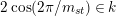
$k\subseteq \mathbb{C}$
with
$2\cos (2\unicode[STIX]{x1D70B}/m_{st})\in k$
for all
$s,t\in S$
and
$p\in k^{\times }$
for all bad primes
$p$
. (See [Reference Geck and Jacon3, Table 1.4] for a detailed description of what that means for each type of finite Coxeter group.)
$k\unicode[STIX]{x1D6FA}$
is finitely generated as a
$k$
-module, where
$k$
is a so-called good ring for
$(W,S)$
; that is, a ring
$k\subseteq \mathbb{C}$
with
$2\cos (2\unicode[STIX]{x1D70B}/m_{st})\in k$
for all
$s,t\in S$
and
$p\in k^{\times }$
for all bad primes
$p$
. (See [Reference Geck and Jacon3, Table 1.4] for a detailed description of what that means for each type of finite Coxeter group.) -
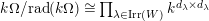
∙ The Jacobson radical
$\text{rad}(k\unicode[STIX]{x1D6FA})$
is finitely generated by an explicitly describable finite list of elements and
$k\unicode[STIX]{x1D6FA}/\text{rad}(k\unicode[STIX]{x1D6FA})\cong \prod _{\unicode[STIX]{x1D706}\in \text{Irr}(W)}k^{d_{\unicode[STIX]{x1D706}}\times d_{\unicode[STIX]{x1D706}}}$
, where
$d_{\unicode[STIX]{x1D706}}$
denotes the degree of the irreducible character
$\unicode[STIX]{x1D706}$
. This implies that Gyoja’s conjecture (cf. [Reference Gyoja4, 2.18]) holds. -
∙ There is an enumeration
$\unicode[STIX]{x1D706}_{1},\ldots ,\unicode[STIX]{x1D706}_{n}$
of
$\text{Irr}(W)$
such that every
$k\unicode[STIX]{x1D6FA}$
-module
$V$
has a natural filtration which realizes the decomposition of
$$\begin{eqnarray}0=V^{0}\subseteq V^{1}\subseteq \cdots \subseteq V^{n}=V,\end{eqnarray}$$
$V$
into irreducibles in the sense that
$V^{i}/V^{i-1}$
is isomorphic to a direct sum of irreducibles of isomorphism class
$\unicode[STIX]{x1D706}_{i}$
.


Because of the last consequence I named the conjecture the “
 $W$
-graph decomposition conjecture”. The second consequence, and in particular the connection to Gyoja’s conjecture, was my original motivation for investigating the
$W$
-graph decomposition conjecture”. The second consequence, and in particular the connection to Gyoja’s conjecture, was my original motivation for investigating the
 $W$
-graph algebra and its fine structure. At the time of writing, the decomposition conjecture has been proven for Coxeter groups of types
$W$
-graph algebra and its fine structure. At the time of writing, the decomposition conjecture has been proven for Coxeter groups of types
 $A_{1}$
–
$A_{1}$
–
 $A_{4}$
,
$A_{4}$
,
 $I_{2}(m)$
and
$I_{2}(m)$
and
 $B_{3}$
.
$B_{3}$
.
The paper is organized as follows. The first section introduces some notation, recalls the definition of
 $W$
-graphs (following [Reference Geck and Jacon3], which is slightly more general than Kazhdan and Lusztig’s), the definition of the
$W$
-graphs (following [Reference Geck and Jacon3], which is slightly more general than Kazhdan and Lusztig’s), the definition of the
 $W$
-graph algebra (following [Reference Gyoja4] though with a different notation) and proves some basic lemmas establishing the connection between
$W$
-graph algebra (following [Reference Gyoja4] though with a different notation) and proves some basic lemmas establishing the connection between
 $W$
-graphs and
$W$
-graphs and
 $\unicode[STIX]{x1D6FA}$
-modules. Section 3 is devoted to stating and proving an explicit description of
$\unicode[STIX]{x1D6FA}$
-modules. Section 3 is devoted to stating and proving an explicit description of
 $\unicode[STIX]{x1D6FA}$
in terms of generators and relations which are the basis for all subsequent proofs. Section 4 contains the statement of the decomposition conjecture and a short discussion of its consequences, while Section 5 is devoted to the proofs of the conjecture for small Coxeter groups.
$\unicode[STIX]{x1D6FA}$
in terms of generators and relations which are the basis for all subsequent proofs. Section 4 contains the statement of the decomposition conjecture and a short discussion of its consequences, while Section 5 is devoted to the proofs of the conjecture for small Coxeter groups.
2 Preliminaries
2.1 Notation
Throughout the paper, fix a finite Coxeter system
 $(W,S)$
. The Iwahori–Hecke algebra
$(W,S)$
. The Iwahori–Hecke algebra
 $H=H(W,S)$
of
$H=H(W,S)$
of
 $(W,S)$
is the
$(W,S)$
is the
 $\mathbb{Z}[v^{\pm 1}]$
-algebra (where
$\mathbb{Z}[v^{\pm 1}]$
-algebra (where
 $v$
is an indeterminate), which is freely generated by
$v$
is an indeterminate), which is freely generated by
 $(T_{s})_{s\in S}$
subject only to the relations
$(T_{s})_{s\in S}$
subject only to the relations
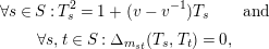 $$\begin{eqnarray}\displaystyle & \displaystyle \forall s\in S:T_{s}^{2}=1+(v-v^{-1})T_{s}\qquad \text{and} & \displaystyle \nonumber\\ \displaystyle & \displaystyle \forall s,t\in S:\unicode[STIX]{x1D6E5}_{m_{st}}(T_{s},T_{t})=0, & \displaystyle \nonumber\end{eqnarray}$$
where
 $m_{st}$
denotes the order of
$m_{st}$
denotes the order of
 $st\in W$
and
$st\in W$
and
 $\unicode[STIX]{x1D6E5}_{m}(x,y)$
is the
$\unicode[STIX]{x1D6E5}_{m}(x,y)$
is the
 $m$
th braid commutator of ring elements
$m$
th braid commutator of ring elements
 $x$
and
$x$
and
 $y$
, which is defined as follows:
$y$
, which is defined as follows:
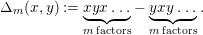 $$\begin{eqnarray}\unicode[STIX]{x1D6E5}_{m}(x,y):=\underbrace{xyx\ldots }_{m\,\text{factors}}-\underbrace{yxy\ldots }_{m\,\text{factors}}.\end{eqnarray}$$
In particular,
 $\unicode[STIX]{x1D6E5}_{0}(x,y)=0$
,
$\unicode[STIX]{x1D6E5}_{0}(x,y)=0$
,
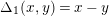 $\unicode[STIX]{x1D6E5}_{1}(x,y)=x-y$
,
$\unicode[STIX]{x1D6E5}_{1}(x,y)=x-y$
,
 $\unicode[STIX]{x1D6E5}_{2}(x,y)=xy-yx$
,
$\unicode[STIX]{x1D6E5}_{2}(x,y)=xy-yx$
,
 $\unicode[STIX]{x1D6E5}_{3}(x,y)=xyx-yxy$
, and so on.
$\unicode[STIX]{x1D6E5}_{3}(x,y)=xyx-yxy$
, and so on.
Also fix a good ring for
 $(W,S)$
; that is, a ring
$(W,S)$
; that is, a ring
 $k\subseteq \mathbb{C}$
with
$k\subseteq \mathbb{C}$
with
 $2\cos (2\unicode[STIX]{x1D70B}/m_{st})\in k$
for all
$2\cos (2\unicode[STIX]{x1D70B}/m_{st})\in k$
for all
 $s,t\in S$
and
$s,t\in S$
and
 $p\in k^{\times }$
for all so-called bad primes
$p\in k^{\times }$
for all so-called bad primes
 $p$
. (See [Reference Geck and Jacon3, Table 1.4] for a detailed description of what that means for each type of finite Coxeter group.)
$p$
. (See [Reference Geck and Jacon3, Table 1.4] for a detailed description of what that means for each type of finite Coxeter group.)
A ring is good if it is big enough for the purposes of representation theory of Coxeter groups. For example, every good field is a splitting field for
 $W$
.
$W$
.
If
 $A$
is a
$A$
is a
 $k$
-algebra and
$k$
-algebra and
 $k^{\prime }$
is a commutative
$k^{\prime }$
is a commutative
 $k$
-algebra, then
$k$
-algebra, then
 $k^{\prime }A$
is used as shorthand for the
$k^{\prime }A$
is used as shorthand for the
 $k^{\prime }$
-algebra
$k^{\prime }$
-algebra
 $k^{\prime }\otimes _{k}A$
. Similarly, the abbreviation
$k^{\prime }\otimes _{k}A$
. Similarly, the abbreviation
 $k^{\prime }V$
is used for the
$k^{\prime }V$
is used for the
 $k^{\prime }A$
-module
$k^{\prime }A$
-module
 $k^{\prime }\otimes _{k}V$
if
$k^{\prime }\otimes _{k}V$
if
 $V$
is an
$V$
is an
 $A$
-module.
$A$
-module.
2.2
$W$
-graphs

Definition 1. (Cf. [Reference Kazhdan and Lusztig7] and [Reference Geck and Jacon3])
A
 $W$
-graph with edge weights in
$W$
-graph with edge weights in
 $k$
is a triple
$k$
is a triple
 $(\mathfrak{C},{\mathcal{I}},m)$
consisting of a finite set
$(\mathfrak{C},{\mathcal{I}},m)$
consisting of a finite set
 $\mathfrak{C}$
of vertices, a vertex labeling map
$\mathfrak{C}$
of vertices, a vertex labeling map
 ${\mathcal{I}}:\mathfrak{C}\rightarrow \{I\mid I\subseteq S\}$
and a family of edge weight matrices
${\mathcal{I}}:\mathfrak{C}\rightarrow \{I\mid I\subseteq S\}$
and a family of edge weight matrices
 $m^{s}\in k^{\mathfrak{C}\times \mathfrak{C}}$
for
$m^{s}\in k^{\mathfrak{C}\times \mathfrak{C}}$
for
 $s\in S$
(here,
$s\in S$
(here,
 $k^{\mathfrak{C}\times \mathfrak{C}}$
denotes the ring of matrices whose rows and columns are indexed with
$k^{\mathfrak{C}\times \mathfrak{C}}$
denotes the ring of matrices whose rows and columns are indexed with
 $\mathfrak{C}$
and whose entries are elements of
$\mathfrak{C}$
and whose entries are elements of
 $k$
) such that the following conditions hold.
$k$
) such that the following conditions hold.
-
(1)
$\forall x,y\in \mathfrak{C}:m_{xy}^{s}\neq 0\;\Longrightarrow \;s\in {\mathcal{I}}(x)\setminus {\mathcal{I}}(y)$
. -
(2) The matrices
induce a matrix representation
$$\begin{eqnarray}\unicode[STIX]{x1D714}(T_{s})_{xy}:=\left\{\begin{array}{@{}ll@{}}-v^{-1}\cdot 1_{k}\quad & \text{if}~x=y,s\in {\mathcal{I}}(x),\\ v\cdot 1_{k}\quad & \text{if}~x=y,s\notin {\mathcal{I}}(x),\\ m_{xy}^{s}\quad & \text{otherwise}\end{array}\right.\end{eqnarray}$$
$\unicode[STIX]{x1D714}:k[v^{\pm 1}]H\rightarrow k[v^{\pm 1}]^{\mathfrak{C}\times \mathfrak{C}}$
.

The associated directed graph is defined as follows. The vertex set is
 $\mathfrak{C}$
and there is a directed edge
$\mathfrak{C}$
and there is a directed edge
 $x\leftarrow y$
if and only if
$x\leftarrow y$
if and only if
 $m_{xy}^{s}\neq 0$
for some
$m_{xy}^{s}\neq 0$
for some
 $s\in S$
. If this is the case, then the value
$s\in S$
. If this is the case, then the value
 $m_{xy}^{s}$
is called the weight of the edge. The set
$m_{xy}^{s}$
is called the weight of the edge. The set
 $I(x)$
is called the vertex label of
$I(x)$
is called the vertex label of
 $x$
.
$x$
.
Note that condition 1 and the definition of
 $\unicode[STIX]{x1D714}(T_{s})$
already guarantee
$\unicode[STIX]{x1D714}(T_{s})$
already guarantee
 $\unicode[STIX]{x1D714}(T_{s})^{2}=1+(v-v^{-1})\unicode[STIX]{x1D714}(T_{s})$
, so that the only nontrivial requirement in condition 2 is the braid relation
$\unicode[STIX]{x1D714}(T_{s})^{2}=1+(v-v^{-1})\unicode[STIX]{x1D714}(T_{s})$
, so that the only nontrivial requirement in condition 2 is the braid relation
 $0=\unicode[STIX]{x1D6E5}_{m_{st}}(\unicode[STIX]{x1D714}(T_{s}),\unicode[STIX]{x1D714}(T_{t}))$
.
$0=\unicode[STIX]{x1D6E5}_{m_{st}}(\unicode[STIX]{x1D714}(T_{s}),\unicode[STIX]{x1D714}(T_{t}))$
.
The definition seems to allow up to
 $|I(x)\setminus I(y)|$
different edge weights for a single edge
$|I(x)\setminus I(y)|$
different edge weights for a single edge
 $x\leftarrow y$
. We prove later that all values
$x\leftarrow y$
. We prove later that all values
 $m_{xy}^{s}$
with
$m_{xy}^{s}$
with
 $s\in I(x)\setminus I(y)$
are in fact equal.
$s\in I(x)\setminus I(y)$
are in fact equal.
Given a
 $W$
-graph as above, the matrix representation
$W$
-graph as above, the matrix representation
 $\unicode[STIX]{x1D714}$
turns the space
$\unicode[STIX]{x1D714}$
turns the space
 $k[v^{\pm 1}]^{\mathfrak{C}}$
of column vectors indexed with
$k[v^{\pm 1}]^{\mathfrak{C}}$
of column vectors indexed with
 $\mathfrak{C}$
with entries in
$\mathfrak{C}$
with entries in
 $k[v^{\pm 1}]$
into a left module for the Hecke algebra
$k[v^{\pm 1}]$
into a left module for the Hecke algebra
 $k[v^{\pm 1}]H$
. It is natural to ask whether the converse is true. In situations where the Hecke algebra is split semisimple, the answer is yes, as shown by Gyoja.
$k[v^{\pm 1}]H$
. It is natural to ask whether the converse is true. In situations where the Hecke algebra is split semisimple, the answer is yes, as shown by Gyoja.
Theorem 2. (Cf. [Reference Gyoja4])
Let
 $K\subseteq \mathbb{C}$
be a splitting field for
$K\subseteq \mathbb{C}$
be a splitting field for
 $W$
. Every irreducible representation of
$W$
. Every irreducible representation of
 $K(v)H$
can be realized as a
$K(v)H$
can be realized as a
 $W$
-graph module for some
$W$
-graph module for some
 $W$
-graph with edge weights in
$W$
-graph with edge weights in
 $K$
.
$K$
.
2.3 Gyoja’s
$W$
-graph algebra

Definition 3. Define
 $\unicode[STIX]{x1D6EF}$
as the
$\unicode[STIX]{x1D6EF}$
as the
 $\mathbb{Z}$
-algebra that is freely generated by
$\mathbb{Z}$
-algebra that is freely generated by
 $e_{s},x_{s}$
for
$e_{s},x_{s}$
for
 $s\in S$
with respect to the following relations:
$s\in S$
with respect to the following relations:
-
(1)
$\forall s\in S:e_{s}^{2}=e_{s}$
; -
(2)
$\forall s,t\in S:e_{s}e_{t}=e_{t}e_{s}$
; -
(3)
$\forall s\in S:e_{s}x_{s}=x_{s},\;x_{s}e_{s}=0$
.


Furthermore, define
 $$\begin{eqnarray}\unicode[STIX]{x1D704}(T_{s}):=-v^{-1}e_{s}+v(1-e_{s})+x_{s}\in \mathbb{Z}[v^{\pm 1}]\unicode[STIX]{x1D6EF}\end{eqnarray}$$
for all
 $s\in S$
. The braid commutator
$s\in S$
. The braid commutator
 $\unicode[STIX]{x1D6E5}_{m_{st}}(\unicode[STIX]{x1D704}(T_{s}),\unicode[STIX]{x1D704}(T_{t}))$
can be written as
$\unicode[STIX]{x1D6E5}_{m_{st}}(\unicode[STIX]{x1D704}(T_{s}),\unicode[STIX]{x1D704}(T_{t}))$
can be written as
 $\sum _{\unicode[STIX]{x1D6FE}\in \mathbb{Z}}y^{\unicode[STIX]{x1D6FE}}(s,t)v^{\unicode[STIX]{x1D6FE}}$
with uniquely determined elements
$\sum _{\unicode[STIX]{x1D6FE}\in \mathbb{Z}}y^{\unicode[STIX]{x1D6FE}}(s,t)v^{\unicode[STIX]{x1D6FE}}$
with uniquely determined elements
 $y^{\unicode[STIX]{x1D6FE}}(s,t)\in \unicode[STIX]{x1D6EF}$
.
$y^{\unicode[STIX]{x1D6FE}}(s,t)\in \unicode[STIX]{x1D6EF}$
.
The
 $W$
-graph algebra
$W$
-graph algebra
 $\unicode[STIX]{x1D6FA}$
is defined as the
$\unicode[STIX]{x1D6FA}$
is defined as the
 $\mathbb{Z}$
-algebra obtained as the quotient of
$\mathbb{Z}$
-algebra obtained as the quotient of
 $\unicode[STIX]{x1D6EF}$
modulo the relations
$\unicode[STIX]{x1D6EF}$
modulo the relations
 $y^{\unicode[STIX]{x1D6FE}}(s,t)=0$
for all
$y^{\unicode[STIX]{x1D6FE}}(s,t)=0$
for all
 $s,t\in S$
and all
$s,t\in S$
and all
 $\unicode[STIX]{x1D6FE}\in \mathbb{Z}$
.
$\unicode[STIX]{x1D6FE}\in \mathbb{Z}$
.
By abuse of notation, the quotient map
 $\unicode[STIX]{x1D6EF}\rightarrow \unicode[STIX]{x1D6FA}$
is not explicitly mentioned for the remainder of this paper, and symbols like
$\unicode[STIX]{x1D6EF}\rightarrow \unicode[STIX]{x1D6FA}$
is not explicitly mentioned for the remainder of this paper, and symbols like
 $e_{s}$
,
$e_{s}$
,
 $x_{s}$
and
$x_{s}$
and
 $\unicode[STIX]{x1D704}(T_{s})$
are therefore used for elements of
$\unicode[STIX]{x1D704}(T_{s})$
are therefore used for elements of
 $\unicode[STIX]{x1D6EF}$
as well as the corresponding elements of
$\unicode[STIX]{x1D6EF}$
as well as the corresponding elements of
 $\unicode[STIX]{x1D6FA}$
.
$\unicode[STIX]{x1D6FA}$
.
The definition, and in particular the observation
 $x_{s}^{2}=(e_{s}x_{s})(e_{s}x_{s})=0$
, immediately implies that
$x_{s}^{2}=(e_{s}x_{s})(e_{s}x_{s})=0$
, immediately implies that
 $T_{s}\mapsto \unicode[STIX]{x1D704}(T_{s})$
defines a homomorphism of
$T_{s}\mapsto \unicode[STIX]{x1D704}(T_{s})$
defines a homomorphism of
 $\mathbb{Z}[v^{\pm 1}]$
-algebras
$\mathbb{Z}[v^{\pm 1}]$
-algebras
 $\unicode[STIX]{x1D704}:H\rightarrow \mathbb{Z}[v^{\pm 1}]\unicode[STIX]{x1D6FA}$
(which is in fact injective, as we prove in Corollary 10). This observation also appears in Gyoja’s paper [Reference Gyoja4, Remark 2.4.3].
$\unicode[STIX]{x1D704}:H\rightarrow \mathbb{Z}[v^{\pm 1}]\unicode[STIX]{x1D6FA}$
(which is in fact injective, as we prove in Corollary 10). This observation also appears in Gyoja’s paper [Reference Gyoja4, Remark 2.4.3].
2.4 Morphisms
Giving an algebra by generators and relations means having a universal property for homomorphisms on the resulting algebra. Since the relations for
 $\unicode[STIX]{x1D6FA}$
are not explicit enough to be verifiable by explicit calculations, we use the following universal property instead.
$\unicode[STIX]{x1D6FA}$
are not explicit enough to be verifiable by explicit calculations, we use the following universal property instead.
Lemma 4. Consider the category of all rings. Then, precomposing with the quotient
 $\unicode[STIX]{x1D6EF}\rightarrow \unicode[STIX]{x1D6FA}$
is a natural isomorphism
$\unicode[STIX]{x1D6EF}\rightarrow \unicode[STIX]{x1D6FA}$
is a natural isomorphism
 $$\begin{eqnarray}\text{Hom}(\unicode[STIX]{x1D6FA},A)\cong \left\{f:\unicode[STIX]{x1D6EF}\rightarrow A\left|\begin{array}{@{}l@{}}\text{the induced map}~\mathbb{Z}[v^{\pm 1}]\unicode[STIX]{x1D6EF}\rightarrow \mathbb{Z}[v^{\pm 1}]A\\ \text{annihilates}~\unicode[STIX]{x1D6E5}_{m_{st}}(\unicode[STIX]{x1D704}(T_{s}),\unicode[STIX]{x1D704}(T_{t}))~\text{for all}~s,t\in S\end{array}\right.\right\}.\end{eqnarray}$$
Proof. Precomposing with the quotient map certainly is an injective natural transformation
 $\text{Hom}(\unicode[STIX]{x1D6FA},-)\rightarrow \text{Hom}(\unicode[STIX]{x1D6EF},-)$
. We prove that its image is exactly the subset of the claim.
$\text{Hom}(\unicode[STIX]{x1D6FA},-)\rightarrow \text{Hom}(\unicode[STIX]{x1D6EF},-)$
. We prove that its image is exactly the subset of the claim.
Choose
 $s,t\in S$
and write
$s,t\in S$
and write
 $\unicode[STIX]{x1D6E5}_{m_{st}}(\unicode[STIX]{x1D704}(T_{s}),\unicode[STIX]{x1D704}(T_{t}))=\sum _{\unicode[STIX]{x1D6FE}\in \mathbb{Z}}y^{\unicode[STIX]{x1D6FE}}(s,t)v^{\unicode[STIX]{x1D6FE}}$
as before. Thus, for any homomorphism
$\unicode[STIX]{x1D6E5}_{m_{st}}(\unicode[STIX]{x1D704}(T_{s}),\unicode[STIX]{x1D704}(T_{t}))=\sum _{\unicode[STIX]{x1D6FE}\in \mathbb{Z}}y^{\unicode[STIX]{x1D6FE}}(s,t)v^{\unicode[STIX]{x1D6FE}}$
as before. Thus, for any homomorphism
 $f:\unicode[STIX]{x1D6EF}\rightarrow A$
, the induced map
$f:\unicode[STIX]{x1D6EF}\rightarrow A$
, the induced map
 $\mathbb{Z}[v^{\pm 1}]\unicode[STIX]{x1D6EF}\rightarrow \mathbb{Z}[v^{\pm 1}]A$
satisfies
$\mathbb{Z}[v^{\pm 1}]\unicode[STIX]{x1D6EF}\rightarrow \mathbb{Z}[v^{\pm 1}]A$
satisfies
 $$\begin{eqnarray}f(\unicode[STIX]{x1D6E5}_{m_{st}}(\unicode[STIX]{x1D704}(T_{s}),\unicode[STIX]{x1D704}(T_{t})))=\mathop{\sum }_{\unicode[STIX]{x1D6FE}\in \mathbb{Z}}f(y^{\unicode[STIX]{x1D6FE}}(s,t))v^{\unicode[STIX]{x1D6FE}}.\end{eqnarray}$$
Because an element
 $\sum _{\unicode[STIX]{x1D6FE}}a_{\unicode[STIX]{x1D6FE}}v^{\unicode[STIX]{x1D6FE}}\in \mathbb{Z}[v^{\pm 1}]A$
with
$\sum _{\unicode[STIX]{x1D6FE}}a_{\unicode[STIX]{x1D6FE}}v^{\unicode[STIX]{x1D6FE}}\in \mathbb{Z}[v^{\pm 1}]A$
with
 $a_{\unicode[STIX]{x1D6FE}}\in A$
is zero if and only if
$a_{\unicode[STIX]{x1D6FE}}\in A$
is zero if and only if
 $a_{\unicode[STIX]{x1D6FE}}=0$
for all
$a_{\unicode[STIX]{x1D6FE}}=0$
for all
 $\unicode[STIX]{x1D6FE}\in \mathbb{Z}$
, the map
$\unicode[STIX]{x1D6FE}\in \mathbb{Z}$
, the map
 $f$
descends to a well-defined homomorphism
$f$
descends to a well-defined homomorphism
 $\unicode[STIX]{x1D6FA}\rightarrow A$
if and only if
$\unicode[STIX]{x1D6FA}\rightarrow A$
if and only if
 $f$
annihilates all
$f$
annihilates all
 $y^{\unicode[STIX]{x1D6FE}}(s,t)$
if and only if the induced map annihilates all braid commutators
$y^{\unicode[STIX]{x1D6FE}}(s,t)$
if and only if the induced map annihilates all braid commutators
 $\unicode[STIX]{x1D6E5}_{m_{st}}(\unicode[STIX]{x1D704}(T_{s}),\unicode[STIX]{x1D704}(T_{t}))$
.◻
$\unicode[STIX]{x1D6E5}_{m_{st}}(\unicode[STIX]{x1D704}(T_{s}),\unicode[STIX]{x1D704}(T_{t}))$
.◻
The following easy corollary establishes symmetries of
 $\unicode[STIX]{x1D6FA}$
which are used to simplify the proofs of the decomposition conjecture in the last section of the paper.
$\unicode[STIX]{x1D6FA}$
which are used to simplify the proofs of the decomposition conjecture in the last section of the paper.
Corollary 5.
-
(1) If
$\unicode[STIX]{x1D6FC}:S\rightarrow S$
is a bijection with
$\text{ord}(\unicode[STIX]{x1D6FC}(s)\unicode[STIX]{x1D6FC}(t))=\text{ord}(st)$
(in other words, a graph automorphism of the Dynkin diagram of
$(W,S)$
), then there is a unique automorphism of
$\unicode[STIX]{x1D6FA}$
with
$e_{s}\mapsto e_{\unicode[STIX]{x1D6FC}(s)}$
,
$x_{s}\mapsto x_{\unicode[STIX]{x1D6FC}(s)}$
. -
(2) There is a unique antiautomorphism
$\unicode[STIX]{x1D6FF}$
of
$\unicode[STIX]{x1D6FA}$
with
$e_{s}\mapsto 1-e_{s}$
,
$x_{s}\mapsto -x_{s}$
.


2.5 Modules and
$W$
-graphs

The following definition appears in Gyoja’s paper [Reference Gyoja4, Definition 2.5], although with different notation.
Definition 6. In
 $\unicode[STIX]{x1D6EF}$
, define the following elements for all
$\unicode[STIX]{x1D6EF}$
, define the following elements for all
 $I,J\subseteq S,s\in S$
:
$I,J\subseteq S,s\in S$
:
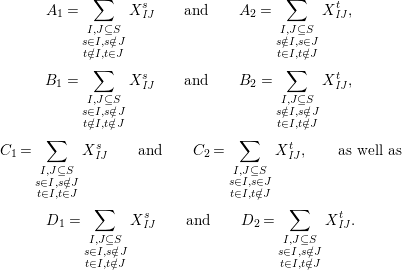
 $$\begin{eqnarray}\displaystyle & \displaystyle E_{I}:=\biggl(\mathop{\prod }_{t\in I}e_{t}\biggr)\biggl(\mathop{\prod }_{t\in S\setminus I}(1-e_{t})\biggr) & \displaystyle \nonumber\\ \displaystyle & \displaystyle X_{\mathit{IJ}}^{s}:=E_{I}x_{s}E_{J}. & \displaystyle \nonumber\end{eqnarray}$$
What Gyoja did not mention in his paper is that these elements actually give
 $\unicode[STIX]{x1D6FA}$
the structure of a quotient of a path algebra. This is the content of the following lemma.
$\unicode[STIX]{x1D6FA}$
the structure of a quotient of a path algebra. This is the content of the following lemma.
Lemma 7. With the above notation, the following statements are true.
-
(1)
$E_{I}E_{J}=\unicode[STIX]{x1D6FF}_{\mathit{IJ}}E_{I}$
,
$\sum _{I\subseteq S}E_{I}=1$
and
$e_{s}=\sum _{\substack{ I\subseteq S \\ s\in I}}E_{I}$
. -
(2)
$X_{\mathit{IJ}}^{s}=0$
if
$s\notin I\setminus J$
and
$x_{s}=\sum _{\substack{ I,J\subseteq S \\ s\in I\setminus J}}X_{\mathit{IJ}}^{s}$
. -
(3)
$\unicode[STIX]{x1D6EF}$
is isomorphic to the path algebra
$\mathbb{Z}{\mathcal{Q}}$
over the quiver
${\mathcal{Q}}$
whose vertex set is the power set of
$S$
and which has exactly
$|I\setminus J|$
edges
$I\leftarrow J$
for every pair of vertices
$I,J\subseteq S$
.


Proof. The first equation follows immediately from the definition,
 $e_{s}(1-e_{s})=(1-e_{s})e_{s}=0$
and the fact that the
$e_{s}(1-e_{s})=(1-e_{s})e_{s}=0$
and the fact that the
 $e_{s}$
commute with each other. The decomposition of the identity follows by expanding
$e_{s}$
commute with each other. The decomposition of the identity follows by expanding
 $1=\prod _{s\in S}(e_{s}+(1-e_{s}))$
, and the expression for
$1=\prod _{s\in S}(e_{s}+(1-e_{s}))$
, and the expression for
 $e_{s}$
follows by applying the decomposition of the identity in
$e_{s}$
follows by applying the decomposition of the identity in
 $e_{s}\cdot 1$
.
$e_{s}\cdot 1$
.
The expression for
 $x_{s}$
follows by applying the decomposition of the identity twice in
$x_{s}$
follows by applying the decomposition of the identity twice in
 $1\cdot x_{s}\cdot 1$
.
$1\cdot x_{s}\cdot 1$
.
The path algebra
 $\mathbb{Z}{\mathcal{Q}}$
can be described as the algebra freely generated by
$\mathbb{Z}{\mathcal{Q}}$
can be described as the algebra freely generated by
 $\{\tilde{E}_{K},\tilde{X}_{\mathit{IJ}}^{s}|K,I,J\subseteq S,s\in I\setminus J\}$
with respect to the relations
$\{\tilde{E}_{K},\tilde{X}_{\mathit{IJ}}^{s}|K,I,J\subseteq S,s\in I\setminus J\}$
with respect to the relations
 $$\begin{eqnarray}\tilde{E}_{I}\tilde{E}_{J}=\unicode[STIX]{x1D6FF}_{\mathit{IJ}}\tilde{E}_{I},\qquad \mathop{\sum }_{I\subseteq S}\tilde{E}_{I}=1\qquad \text{and}\qquad \tilde{X}_{\mathit{IJ}}^{s}=\tilde{E}_{I}\tilde{X}_{\mathit{IJ}}^{s}\tilde{E}_{J}.\end{eqnarray}$$
This implies that
 $\tilde{E}_{I}\mapsto E_{I}$
,
$\tilde{E}_{I}\mapsto E_{I}$
,
 $\tilde{X}_{\mathit{IJ}}^{s}\mapsto X_{\mathit{IJ}}^{s}$
induces a ring homomorphism
$\tilde{X}_{\mathit{IJ}}^{s}\mapsto X_{\mathit{IJ}}^{s}$
induces a ring homomorphism
 $\mathbb{Z}{\mathcal{Q}}\rightarrow \unicode[STIX]{x1D6EF}$
. Going in the other direction, one readily verifies that the unique ring homomorphism
$\mathbb{Z}{\mathcal{Q}}\rightarrow \unicode[STIX]{x1D6EF}$
. Going in the other direction, one readily verifies that the unique ring homomorphism
 $\unicode[STIX]{x1D6EF}\rightarrow \mathbb{Z}{\mathcal{Q}}$
with
$\unicode[STIX]{x1D6EF}\rightarrow \mathbb{Z}{\mathcal{Q}}$
with
 $e_{s}\mapsto \sum _{\substack{ I\subseteq S \\ s\in I}}\tilde{E}_{I}$
and
$e_{s}\mapsto \sum _{\substack{ I\subseteq S \\ s\in I}}\tilde{E}_{I}$
and
 $x_{s}\mapsto \sum _{\substack{ I,J\subseteq S \\ s\in I\setminus J}}\tilde{X}_{\mathit{IJ}}^{s}$
is inverse to the first morphism.◻
$x_{s}\mapsto \sum _{\substack{ I,J\subseteq S \\ s\in I\setminus J}}\tilde{X}_{\mathit{IJ}}^{s}$
is inverse to the first morphism.◻
Remark 8. For later use, we observe the following.
-
(1) The algebra automorphism induced by a graph automorphism
$\unicode[STIX]{x1D6FC}$
maps
$E_{I}\mapsto E_{\unicode[STIX]{x1D6FC}(I)}$
and
$X_{\mathit{IJ}}^{s}\mapsto X_{\unicode[STIX]{x1D6FC}(I)\unicode[STIX]{x1D6FC}(J)}^{\unicode[STIX]{x1D6FC}(s)}$
. -
(2) The antiautomorphism
$\unicode[STIX]{x1D6FF}$
maps
$E_{I}\mapsto E_{I^{c}}$
and
$X_{\mathit{IJ}}^{s}\mapsto -X_{J^{c}I^{c}}^{s}$
, where
$I^{c}$
denotes the complement of
$I$
in
$S$
.


The following theorem also appears in Gyoja’s paper as a remark without proof and establishes the connection between
 $\unicode[STIX]{x1D6FA}$
and
$\unicode[STIX]{x1D6FA}$
and
 $W$
-graphs.
$W$
-graphs.
Theorem 9. (Cf. [Reference Gyoja4, Remark 2.7])
Let
 $k$
be a commutative ring. There is a correspondence between
$k$
be a commutative ring. There is a correspondence between
 $\unicode[STIX]{x1D6FA}$
-modules and
$\unicode[STIX]{x1D6FA}$
-modules and
 $W$
-graphs by the choice of a suitable basis. More precisely, the following statements hold.
$W$
-graphs by the choice of a suitable basis. More precisely, the following statements hold.
-
(1) (From
$W$
-graphs to
$\unicode[STIX]{x1D6FA}$
-modules)Let
$(\mathfrak{C},{\mathcal{I}},m)$
be a
$W$
-graph with edge weights in
$k$
. Define
$\unicode[STIX]{x1D714}:k\unicode[STIX]{x1D6FA}\rightarrow k^{\mathfrak{C}\times \mathfrak{C}}$
by Then,
$$\begin{eqnarray}\unicode[STIX]{x1D714}(e_{s})_{xy}:=\left\{\begin{array}{@{}ll@{}}1\quad & x=y,s\in {\mathcal{I}}(x)\\ 0\quad & \text{otherwise}\end{array}\right.\qquad \text{and}\qquad \unicode[STIX]{x1D714}(x_{s}):=m^{s}.\end{eqnarray}$$
$\unicode[STIX]{x1D714}$
is a well-defined
$k$
-algebra homomorphism such that the composition is exactly the matrix representation of
$$\begin{eqnarray}k[v^{\pm 1}]H\xrightarrow[{}]{\unicode[STIX]{x1D704}}k[v^{\pm 1}]\unicode[STIX]{x1D6FA}\xrightarrow[{}]{\unicode[STIX]{x1D714}}k[v^{\pm 1}]^{\mathfrak{C}\times \mathfrak{C}}\end{eqnarray}$$
$H$
attached to
$(\mathfrak{C},{\mathcal{I}},m)$
.
-
(2) (From
$\unicode[STIX]{x1D6FA}$
-modules to
$W$
-graphs)Let
$V$
be a
$k\unicode[STIX]{x1D6FA}$
-module with representation
$\unicode[STIX]{x1D714}:k\unicode[STIX]{x1D6FA}\rightarrow \operatorname{End}_{k}(V)$
. Define
$V_{I}:=E_{I}V$
for all
$I\subseteq S$
.If
$V_{I}$
is a finitely generated free
$k$
-module and
$\mathfrak{C}_{I}\subseteq V_{I}$
is a
$k$
-basis for all
$I\subseteq S$
, define
$(\mathfrak{C},{\mathcal{I}},m)$
as follows: set
$\mathfrak{C}:=\bigcup _{I\subseteq S}\mathfrak{C}_{I}$
, set
${\mathcal{I}}(x):=I$
for all
$x\in \mathfrak{C}_{I}$
and define
$m^{s}$
to be the matrix of
$\unicode[STIX]{x1D714}(x_{s})$
with respect to the basis
$\mathfrak{C}$
. With these definitions,
$(\mathfrak{C},{\mathcal{I}},m)$
is a
$W$
-graph and its
$W$
-graph module is
$k[v^{\pm 1}]\otimes _{k}V$
.


Proof. (1) The matrices
 $\unicode[STIX]{x1D714}(e_{s})$
and
$\unicode[STIX]{x1D714}(e_{s})$
and
 $\unicode[STIX]{x1D714}(x_{s})$
satisfy the relations of
$\unicode[STIX]{x1D714}(x_{s})$
satisfy the relations of
 $\unicode[STIX]{x1D6EF}$
by definition of
$\unicode[STIX]{x1D6EF}$
by definition of
 $W$
-graphs. We therefore view
$W$
-graphs. We therefore view
 $\unicode[STIX]{x1D714}$
as an algebra homomorphism
$\unicode[STIX]{x1D714}$
as an algebra homomorphism
 $\unicode[STIX]{x1D6EF}\rightarrow k^{\mathfrak{C}\times \mathfrak{C}}$
. Because
$\unicode[STIX]{x1D6EF}\rightarrow k^{\mathfrak{C}\times \mathfrak{C}}$
. Because
 $\unicode[STIX]{x1D714}(\unicode[STIX]{x1D704}(T_{s}))$
is exactly equal to the matrices
$\unicode[STIX]{x1D714}(\unicode[STIX]{x1D704}(T_{s}))$
is exactly equal to the matrices
 $\unicode[STIX]{x1D714}(T_{s})$
in the definition of
$\unicode[STIX]{x1D714}(T_{s})$
in the definition of
 $W$
-graphs, and those matrices satisfy the braid relations, it follows that
$W$
-graphs, and those matrices satisfy the braid relations, it follows that
 $\unicode[STIX]{x1D714}$
descends to a homomorphism
$\unicode[STIX]{x1D714}$
descends to a homomorphism
 $\unicode[STIX]{x1D6FA}\rightarrow k^{\mathfrak{C}\times \mathfrak{C}}$
by the universal property.
$\unicode[STIX]{x1D6FA}\rightarrow k^{\mathfrak{C}\times \mathfrak{C}}$
by the universal property.
(2) The second assertion is easily verified. The condition
 $m_{xy}^{s}\neq 0\;\Longrightarrow \;s\in {\mathcal{I}}(x)\setminus {\mathcal{I}}(y)$
follows from
$m_{xy}^{s}\neq 0\;\Longrightarrow \;s\in {\mathcal{I}}(x)\setminus {\mathcal{I}}(y)$
follows from
 $X_{\mathit{IJ}}^{s}\neq 0\;\Longrightarrow \;s\in I\setminus J$
. The matrices occurring in the definition of
$X_{\mathit{IJ}}^{s}\neq 0\;\Longrightarrow \;s\in I\setminus J$
. The matrices occurring in the definition of
 $W$
-graphs are exactly the matrices
$W$
-graphs are exactly the matrices
 $\unicode[STIX]{x1D714}(\unicode[STIX]{x1D704}(T_{s}))$
, and hence satisfy the necessary braid relations because the elements
$\unicode[STIX]{x1D714}(\unicode[STIX]{x1D704}(T_{s}))$
, and hence satisfy the necessary braid relations because the elements
 $\unicode[STIX]{x1D704}(T_{s})\in \unicode[STIX]{x1D6FA}$
satisfy them.◻
$\unicode[STIX]{x1D704}(T_{s})\in \unicode[STIX]{x1D6FA}$
satisfy them.◻
Corollary 10. If
 $W$
is finite, then the following hold.
$W$
is finite, then the following hold.
-
(1)
$\unicode[STIX]{x1D704}:k[v^{\pm 1}]H\rightarrow k[v^{\pm 1}]\unicode[STIX]{x1D6FA}$
is injective. -
(2) All
$E_{I}$
are nonzero as elements of
$k\unicode[STIX]{x1D6FA}$
.


In particular,
 $H$
is considered as a subalgebra of the scalar extension
$H$
is considered as a subalgebra of the scalar extension
 $\mathbb{Z}[v^{\pm 1}]\unicode[STIX]{x1D6FA}$
for the rest of this paper.
$\mathbb{Z}[v^{\pm 1}]\unicode[STIX]{x1D6FA}$
for the rest of this paper.
Proof. Consider the Kazhdan–Lusztig-
 $W$
-graph as defined in [Reference Kazhdan and Lusztig7]. It is a
$W$
-graph as defined in [Reference Kazhdan and Lusztig7]. It is a
 $W$
-graph
$W$
-graph
 $(\mathfrak{C},{\mathcal{I}},m)$
with
$(\mathfrak{C},{\mathcal{I}},m)$
with
 $\mathfrak{C}:=W$
,
$\mathfrak{C}:=W$
,
 ${\mathcal{I}}(w):=\{s\in S\mid sw<w\}$
and integer edge weights such that the associated
${\mathcal{I}}(w):=\{s\in S\mid sw<w\}$
and integer edge weights such that the associated
 $W$
-graph module is the regular
$W$
-graph module is the regular
 $H$
-module. This can be considered as a
$H$
-module. This can be considered as a
 $W$
-graph with edge weights in
$W$
-graph with edge weights in
 $k$
.
$k$
.
The representation
 $k[v^{\pm 1}]H\xrightarrow[{}]{\unicode[STIX]{x1D704}}k[v^{\pm 1}]\unicode[STIX]{x1D6FA}\rightarrow k[v^{\pm 1}]^{W\times W}$
induced by this
$k[v^{\pm 1}]H\xrightarrow[{}]{\unicode[STIX]{x1D704}}k[v^{\pm 1}]\unicode[STIX]{x1D6FA}\rightarrow k[v^{\pm 1}]^{W\times W}$
induced by this
 $W$
-graph equals the map
$W$
-graph equals the map
 $k[v^{\pm 1}]H\rightarrow \text{End}_{k[v^{\pm 1}]}(k[v^{\pm 1}]H)$
,
$k[v^{\pm 1}]H\rightarrow \text{End}_{k[v^{\pm 1}]}(k[v^{\pm 1}]H)$
,
 $h\mapsto (x\mapsto hx)$
. The latter map is injective, so that
$h\mapsto (x\mapsto hx)$
. The latter map is injective, so that
 $\unicode[STIX]{x1D704}:k[v^{\pm 1}]H\rightarrow k[v^{\pm 1}]\unicode[STIX]{x1D6FA}$
is injective too.
$\unicode[STIX]{x1D704}:k[v^{\pm 1}]H\rightarrow k[v^{\pm 1}]\unicode[STIX]{x1D6FA}$
is injective too.
If
 $W$
is finite, then all the elements
$W$
is finite, then all the elements
 $E_{I}\in k\unicode[STIX]{x1D6FA}$
are nonzero because there are
$E_{I}\in k\unicode[STIX]{x1D6FA}$
are nonzero because there are
 $w\in \mathfrak{C}$
with
$w\in \mathfrak{C}$
with
 ${\mathcal{I}}(w)=I$
(for example, the longest elements of the corresponding parabolic subgroup
${\mathcal{I}}(w)=I$
(for example, the longest elements of the corresponding parabolic subgroup
 $W_{I}$
).◻
$W_{I}$
).◻
Remark 11. The finiteness condition is in fact superfluous. A more carefully phrased version of the definition of
 $W$
-graphs and of Theorem 9 which also includes the infinite-dimensional case makes the same proof work for the first statement. The second statement, however, cannot be proved in the same way because there is an element
$W$
-graphs and of Theorem 9 which also includes the infinite-dimensional case makes the same proof work for the first statement. The second statement, however, cannot be proved in the same way because there is an element
 $w\in W$
with
$w\in W$
with
 ${\mathcal{I}}(w)=I$
if and only if
${\mathcal{I}}(w)=I$
if and only if
 $W_{I}$
is finite, so that this proof does not work for infinite Coxeter groups (contrary to what I believed when I wrote my thesis, which contains the special proof for the general statement). An alternative general proof of the second statement will be contained in my next paper [Reference Hahn6].
$W_{I}$
is finite, so that this proof does not work for infinite Coxeter groups (contrary to what I believed when I wrote my thesis, which contains the special proof for the general statement). An alternative general proof of the second statement will be contained in my next paper [Reference Hahn6].
3
$\unicode[STIX]{x1D6FA}$
as a quotient of a path algebra

It is observed in Lemma 7 that
 $\unicode[STIX]{x1D6EF}$
is a path algebra. In this section, we give an explicit set of relations for the quotient
$\unicode[STIX]{x1D6EF}$
is a path algebra. In this section, we give an explicit set of relations for the quotient
 $\unicode[STIX]{x1D6EF}\rightarrow \unicode[STIX]{x1D6FA}$
in terms of this path algebra structure. The proof is inspired by equations appearing in Stembridge’s paper [Reference Stembridge8].
$\unicode[STIX]{x1D6EF}\rightarrow \unicode[STIX]{x1D6FA}$
in terms of this path algebra structure. The proof is inspired by equations appearing in Stembridge’s paper [Reference Stembridge8].
We need the following lemma, which is a slight generalization of [Reference Stembridge8, Proposition 3.1].
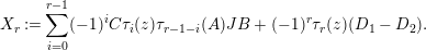
Lemma 12. Define polynomials
 $\unicode[STIX]{x1D70F}_{r}\in \mathbb{Z}[T]$
by the following recursion:
$\unicode[STIX]{x1D70F}_{r}\in \mathbb{Z}[T]$
by the following recursion:
 $$\begin{eqnarray}\unicode[STIX]{x1D70F}_{-1}:=0,\qquad \unicode[STIX]{x1D70F}_{0}:=1,\qquad \unicode[STIX]{x1D70F}_{r}:=T\unicode[STIX]{x1D70F}_{r-1}-\unicode[STIX]{x1D70F}_{r-2}.\end{eqnarray}$$
With this notation the following holds.
If
 $R$
is any ring, and
$R$
is any ring, and
 $x,y\in R$
are solutions of the equation
$x,y\in R$
are solutions of the equation
 $T^{2}=1+\unicode[STIX]{x1D701}T$
for some fixed
$T^{2}=1+\unicode[STIX]{x1D701}T$
for some fixed
 $\unicode[STIX]{x1D701}\in R$
, then their braid commutators satisfy
$\unicode[STIX]{x1D701}\in R$
, then their braid commutators satisfy
 $$\begin{eqnarray}\unicode[STIX]{x1D6E5}_{r+1}(x,y)=(-1)^{r}\unicode[STIX]{x1D70F}_{r}(x+y-\unicode[STIX]{x1D701})\cdot (x-y).\end{eqnarray}$$
Observe that
 $\unicode[STIX]{x1D70F}_{r}$
is a monic polynomial of degree
$\unicode[STIX]{x1D70F}_{r}$
is a monic polynomial of degree
 $r$
for all
$r$
for all
 $r\in \mathbb{N}$
. In particular,
$r\in \mathbb{N}$
. In particular,
 $\{\unicode[STIX]{x1D70F}_{0},\ldots ,\unicode[STIX]{x1D70F}_{r}\}$
is a
$\{\unicode[STIX]{x1D70F}_{0},\ldots ,\unicode[STIX]{x1D70F}_{r}\}$
is a
 $\mathbb{Z}$
-basis of
$\mathbb{Z}$
-basis of
 $\{f\in \mathbb{Z}[T]\mid \deg (f)\leqslant r\}$
. Furthermore,
$\{f\in \mathbb{Z}[T]\mid \deg (f)\leqslant r\}$
. Furthermore,
 $\unicode[STIX]{x1D70F}_{r}$
is an even polynomial for even
$\unicode[STIX]{x1D70F}_{r}$
is an even polynomial for even
 $r$
and an odd polynomial for odd
$r$
and an odd polynomial for odd
 $r$
; that is,
$r$
; that is,
 $\unicode[STIX]{x1D70F}_{r}(-T)=(-1)^{r}\unicode[STIX]{x1D70F}_{r}(T)$
. This follows immediately from the recursion.
$\unicode[STIX]{x1D70F}_{r}(-T)=(-1)^{r}\unicode[STIX]{x1D70F}_{r}(T)$
. This follows immediately from the recursion.
Proof. The claim for the braid commutator is true for
 $r=-1$
and
$r=-1$
and
 $r=0$
. Furthermore, the following holds:
$r=0$
. Furthermore, the following holds:
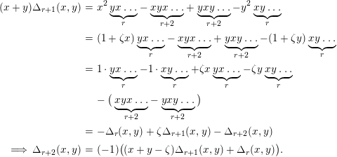 $$\begin{eqnarray}\displaystyle (x+y)\unicode[STIX]{x1D6E5}_{r+1}(x,y) & = & \displaystyle x^{2}\underbrace{yx\ldots }_{r}-\underbrace{xyx\ldots }_{r+2}+\underbrace{yxy\ldots }_{r+2}-y^{2}\underbrace{xy\ldots }_{r}\nonumber\\ \displaystyle & = & \displaystyle (1+\unicode[STIX]{x1D701}x)\underbrace{yx\ldots }_{r}-\underbrace{xyx\ldots }_{r+2}+\underbrace{yxy\ldots }_{r+2}-(1+\unicode[STIX]{x1D701}y)\underbrace{xy\ldots }_{r}\nonumber\\ \displaystyle & = & \displaystyle 1\cdot \underbrace{yx\ldots }_{r}-1\cdot \underbrace{xy\ldots }_{r}+\unicode[STIX]{x1D701}x\underbrace{yx\ldots }_{r}-\unicode[STIX]{x1D701}y\underbrace{xy\ldots }_{r}\nonumber\\ \displaystyle & & \displaystyle -\,\big(\underbrace{xyx\ldots }_{r+2}-\underbrace{yxy\ldots }_{r+2}\big)\nonumber\\ \displaystyle & = & \displaystyle -\unicode[STIX]{x1D6E5}_{r}(x,y)+\unicode[STIX]{x1D701}\unicode[STIX]{x1D6E5}_{r+1}(x,y)-\unicode[STIX]{x1D6E5}_{r+2}(x,y)\nonumber\\ \displaystyle \;\Longrightarrow \;\unicode[STIX]{x1D6E5}_{r+2}(x,y) & = & \displaystyle (-1)\big((x+y-\unicode[STIX]{x1D701})\unicode[STIX]{x1D6E5}_{r+1}(x,y)+\unicode[STIX]{x1D6E5}_{r}(x,y)\big).\nonumber\end{eqnarray}$$
The claim follows by induction. ◻
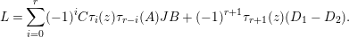
Theorem 13. For all
 $I,J\subseteq S$
,
$I,J\subseteq S$
,
 $s,t\in S$
and
$s,t\in S$
and
 $r\in \mathbb{N}$
, define
$r\in \mathbb{N}$
, define
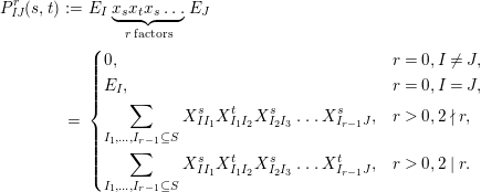 $$\begin{eqnarray}\displaystyle P_{\mathit{IJ}}^{r}(s,t) & := & \displaystyle E_{I}\underbrace{x_{s}x_{t}x_{s}\ldots }_{r\,\text{factors}}E_{J}\nonumber\\ \displaystyle & = & \displaystyle \left\{\begin{array}{@{}ll@{}}0,\quad & r=0,I\neq J,\\ E_{I},\quad & r=0,I=J,\\ \displaystyle \mathop{\sum }_{I_{1},\ldots ,I_{r-1}\subseteq S}X_{II_{1}}^{s}X_{I_{1}I_{2}}^{t}X_{I_{2}I_{3}}^{s}\ldots X_{I_{r-1}J}^{s},\quad & r>0,2\nmid r,\\ \displaystyle \mathop{\sum }_{I_{1},\ldots ,I_{r-1}\subseteq S}X_{II_{1}}^{s}X_{I_{1}I_{2}}^{t}X_{I_{2}I_{3}}^{s}\ldots X_{I_{r-1}J}^{t},\quad & r>0,2\mid r.\end{array}\right.\nonumber\end{eqnarray}$$
With this notation, the kernel of the quotient
 $\unicode[STIX]{x1D6EF}\rightarrow \unicode[STIX]{x1D6FA}$
is generated by the following elements.
$\unicode[STIX]{x1D6EF}\rightarrow \unicode[STIX]{x1D6FA}$
is generated by the following elements.
-
(α) For all
$s,t\in S$
, the elements for all
$$\begin{eqnarray}P_{\mathit{IJ}}^{m-1}(s,t)+a_{m-2}P_{\mathit{IJ}}^{m-2}(s,t)+\cdots +a_{1}P_{\mathit{IJ}}^{1}(s,t)+a_{0}P_{\mathit{IJ}}^{0}(s,t)\end{eqnarray}$$
$I,J\subseteq S$
, where either
-
∙
$s\in I$
,
$t\notin I$
,
$s\in J$
,
$t\notin J$
and
$2\nmid m_{st}$
or -
∙
$s\in I$
,
$t\notin I$
,
$s\notin J$
,
$t\in J$
and
$2\mid m_{st}$
holds. The
$a_{i}$
denote the coefficients of the polynomial
$\unicode[STIX]{x1D70F}_{m-1}$
; that is,
$$\begin{eqnarray}\unicode[STIX]{x1D70F}_{m-1}(T)=T^{m-1}+a_{m-2}T^{m-2}+\cdots +a_{1}T+a_{0}.\end{eqnarray}$$
-


-
(β) For all
$s,t\in S$
and all
$I,J\subseteq S$
with
$s,t\in I\setminus J$
, the elements
$$\begin{eqnarray}P_{\mathit{IJ}}^{1}(s,t)-P_{\mathit{IJ}}^{1}(t,s),P_{\mathit{IJ}}^{2}(s,t)-P_{\mathit{IJ}}^{2}(t,s),\ldots ,P_{\mathit{IJ}}^{m}(s,t)-P_{\mathit{IJ}}^{m}(t,s).\end{eqnarray}$$


These relations are used throughout the rest of the paper. We refer to them as the
 $(\unicode[STIX]{x1D6FC}^{st})$
-relation and the
$(\unicode[STIX]{x1D6FC}^{st})$
-relation and the
 $(\unicode[STIX]{x1D6FD}^{st})$
-relation, respectively.
$(\unicode[STIX]{x1D6FD}^{st})$
-relation, respectively.
Proof. Consider
 $V:=\mathbb{Z}[v^{\pm 1}]\unicode[STIX]{x1D6EF}$
and fixed
$V:=\mathbb{Z}[v^{\pm 1}]\unicode[STIX]{x1D6EF}$
and fixed
 $s,t\in S$
. Define the four subspaces
$s,t\in S$
. Define the four subspaces
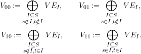 $$\begin{eqnarray}\displaystyle & \displaystyle V_{00}:=\bigoplus _{\substack{ I\subseteq S \\ s\notin I,t\notin I}}VE_{I},\qquad V_{01}:=\bigoplus _{\substack{ I\subseteq S \\ s\in I,t\notin I}}VE_{I}, & \displaystyle \nonumber\\ \displaystyle & \displaystyle V_{10}:=\bigoplus _{\substack{ I\subseteq S \\ s\notin I,t\in I}}VE_{I},\qquad V_{11}:=\bigoplus _{\substack{ I\subseteq S \\ s\in I,t\in I}}VE_{I}. & \displaystyle \nonumber\end{eqnarray}$$
Note that, given an algebra
 $A$
and a decomposition into pairwise orthogonal idempotents
$A$
and a decomposition into pairwise orthogonal idempotents
 $1_{A}=\sum _{i=1}^{n}e_{i}$
, every element
$1_{A}=\sum _{i=1}^{n}e_{i}$
, every element
 $a\in A$
can be uniquely written as
$a\in A$
can be uniquely written as
 $a=\sum _{i,j}a_{ij}$
, with
$a=\sum _{i,j}a_{ij}$
, with
 $a_{ij}\in e_{i}Ae_{j}$
, and this additive decomposition behaves like matrices behave with respect to multiplication; that is,
$a_{ij}\in e_{i}Ae_{j}$
, and this additive decomposition behaves like matrices behave with respect to multiplication; that is,
 $(ab)_{ik}=\sum _{j}a_{ij}b_{jk}$
.
$(ab)_{ik}=\sum _{j}a_{ij}b_{jk}$
.
We therefore write elements of
 $\mathbb{Z}[v^{\pm 1}]\unicode[STIX]{x1D6EF}$
as matrices when we want to display such a decomposition in an efficient way. Note that one can view these matrices equivalently either as
$\mathbb{Z}[v^{\pm 1}]\unicode[STIX]{x1D6EF}$
as matrices when we want to display such a decomposition in an efficient way. Note that one can view these matrices equivalently either as
 $d\times d$
-matrices with entries in the Laurent polynomial ring
$d\times d$
-matrices with entries in the Laurent polynomial ring
 $\mathbb{Z}[v^{\pm 1}]\unicode[STIX]{x1D6EF}$
or as Laurent polynomials over the matrix ring
$\mathbb{Z}[v^{\pm 1}]\unicode[STIX]{x1D6EF}$
or as Laurent polynomials over the matrix ring
 $\unicode[STIX]{x1D6EF}^{d\times d}$
. In other words,
$\unicode[STIX]{x1D6EF}^{d\times d}$
. In other words,
 $\mathbb{Z}[v^{\pm 1}]\otimes (\unicode[STIX]{x1D6EF}^{d\times d})=(\mathbb{Z}[v^{\pm 1}]\otimes \unicode[STIX]{x1D6EF})^{d\times d}$
. It is therefore sensible to speak of the coefficient of
$\mathbb{Z}[v^{\pm 1}]\otimes (\unicode[STIX]{x1D6EF}^{d\times d})=(\mathbb{Z}[v^{\pm 1}]\otimes \unicode[STIX]{x1D6EF})^{d\times d}$
. It is therefore sensible to speak of the coefficient of
 $v^{k}$
of a matrix.
$v^{k}$
of a matrix.
The matrices of
 $\unicode[STIX]{x1D704}(T_{s})=-v^{-1}e_{s}+x_{s}+v(1-e_{s})$
and
$\unicode[STIX]{x1D704}(T_{s})=-v^{-1}e_{s}+x_{s}+v(1-e_{s})$
and
 $\unicode[STIX]{x1D704}(T_{t})$
are given by
$\unicode[STIX]{x1D704}(T_{t})$
are given by
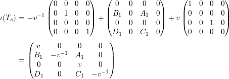 $$\begin{eqnarray}\displaystyle \unicode[STIX]{x1D704}(T_{s}) & = & \displaystyle -v^{-1}\left(\begin{array}{@{}cccc@{}}0 & 0 & 0 & 0\\ 0 & 1 & 0 & 0\\ 0 & 0 & 0 & 0\\ 0 & 0 & 0 & 1\end{array}\right)+\left(\begin{array}{@{}cccc@{}}0 & 0 & 0 & 0\\ B_{1} & 0 & A_{1} & 0\\ 0 & 0 & 0 & 0\\ D_{1} & 0 & C_{1} & 0\end{array}\right)+v\left(\begin{array}{@{}cccc@{}}1 & 0 & 0 & 0\\ 0 & 0 & 0 & 0\\ 0 & 0 & 1 & 0\\ 0 & 0 & 0 & 0\end{array}\right)\nonumber\\ \displaystyle & = & \displaystyle \left(\begin{array}{@{}cccc@{}}v & 0 & 0 & 0\\ B_{1} & -v^{-1} & A_{1} & 0\\ 0 & 0 & v & 0\\ D_{1} & 0 & C_{1} & -v^{-1}\end{array}\right)\nonumber\end{eqnarray}$$
and
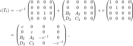 $$\begin{eqnarray}\displaystyle \unicode[STIX]{x1D704}(T_{t}) & = & \displaystyle -v^{-1}\left(\begin{array}{@{}cccc@{}}0 & 0 & 0 & 0\\ 0 & 0 & 0 & 0\\ 0 & 0 & 1 & 0\\ 0 & 0 & 0 & 1\end{array}\right)+\left(\begin{array}{@{}cccc@{}}0 & 0 & 0 & 0\\ 0 & 0 & 0 & 0\\ B_{2} & A_{2} & 0 & 0\\ D_{2} & C_{2} & 0 & 0\end{array}\right)+v\left(\begin{array}{@{}cccc@{}}1 & 0 & 0 & 0\\ 0 & 1 & 0 & 0\\ 0 & 0 & 0 & 0\\ 0 & 0 & 0 & 0\end{array}\right)\nonumber\\ \displaystyle & = & \displaystyle \left(\begin{array}{@{}cccc@{}}v & 0 & 0 & 0\\ 0 & v & 0 & 0\\ B_{2} & A_{2} & -v^{-1} & 0\\ D_{2} & C_{2} & 0 & -v^{-1}\end{array}\right),\nonumber\end{eqnarray}$$
respectively, where
 $$\begin{eqnarray}\displaystyle & \displaystyle A_{1}=\mathop{\sum }_{\substack{ I,J\subseteq S \\ s\in I,s\notin J \\ t\notin I,t\in J}}X_{\mathit{IJ}}^{s}\qquad \text{and}\qquad A_{2}=\mathop{\sum }_{\substack{ I,J\subseteq S \\ s\notin I,s\in J \\ t\in I,t\notin J}}X_{\mathit{IJ}}^{t}, & \displaystyle \nonumber\\ \displaystyle & \displaystyle B_{1}=\mathop{\sum }_{\substack{ I,J\subseteq S \\ s\in I,s\notin J \\ t\notin I,t\notin J}}X_{\mathit{IJ}}^{s}\qquad \text{and}\qquad B_{2}=\mathop{\sum }_{\substack{ I,J\subseteq S \\ s\notin I,s\notin J \\ t\in I,t\notin J}}X_{\mathit{IJ}}^{t}, & \displaystyle \nonumber\\ \displaystyle & \displaystyle C_{1}=\mathop{\sum }_{\substack{ I,J\subseteq S \\ s\in I,s\notin J \\ t\in I,t\in J}}X_{\mathit{IJ}}^{s}\qquad \text{and}\qquad C_{2}=\mathop{\sum }_{\substack{ I,J\subseteq S \\ s\in I,s\in J \\ t\in I,t\notin J}}X_{\mathit{IJ}}^{t},\qquad \text{as well as} & \displaystyle \nonumber\\ \displaystyle & \displaystyle D_{1}=\mathop{\sum }_{\substack{ I,J\subseteq S \\ s\in I,s\notin J \\ t\in I,t\notin J}}X_{\mathit{IJ}}^{s}\qquad \text{and}\qquad D_{2}=\mathop{\sum }_{\substack{ I,J\subseteq S \\ s\in I,s\notin J \\ t\in I,t\notin J}}X_{\mathit{IJ}}^{t}. & \displaystyle \nonumber\end{eqnarray}$$
Finally, define
 $z$
to be
$z$
to be
 $v+v^{-1}$
.
$v+v^{-1}$
.
Step 1. We claim that for all
 $r\in \mathbb{N}$
,
$r\in \mathbb{N}$
,
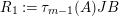
 $$\begin{eqnarray}\unicode[STIX]{x1D6E5}_{r+1}(\unicode[STIX]{x1D704}(T_{s}),\unicode[STIX]{x1D704}(T_{t}))=(-1)^{r}\left(\begin{array}{@{}ccc@{}}0 & 0 & 0\\ \unicode[STIX]{x1D70F}_{r}(A)JB & \unicode[STIX]{x1D70F}_{r}(A)J(A-z) & 0\\ X_{r} & -C\unicode[STIX]{x1D70F}_{r}(A)J & 0\end{array}\right)\end{eqnarray}$$
holds, where
 $$\begin{eqnarray}\displaystyle & \displaystyle A:=\left(\begin{array}{@{}cc@{}}0 & A_{1}\\ A_{2} & 0\end{array}\right)\!,\qquad B:=\left(\begin{array}{@{}c@{}}B_{1}\\ B_{2}\end{array}\right)\!,\qquad C:=\left(\begin{array}{@{}cc@{}}C_{2} & C_{1}\end{array}\right)\!,\qquad J:=\left(\begin{array}{@{}cc@{}}1 & 0\\ 0 & -1\end{array}\right) & \displaystyle \nonumber\end{eqnarray}$$
and
 $$\begin{eqnarray}\displaystyle & \displaystyle X_{r}:=\mathop{\sum }_{i=0}^{r-1}(-1)^{i}C\unicode[STIX]{x1D70F}_{i}(z)\unicode[STIX]{x1D70F}_{r-1-i}(A)JB+(-1)^{r}\unicode[STIX]{x1D70F}_{r}(z)(D_{1}-D_{2}). & \displaystyle \nonumber\end{eqnarray}$$
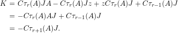
In order to prove this claim, define
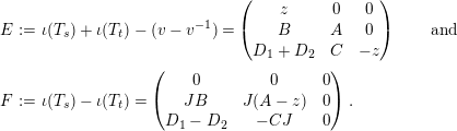 $$\begin{eqnarray}\displaystyle E & := & \displaystyle \unicode[STIX]{x1D704}(T_{s})+\unicode[STIX]{x1D704}(T_{t})-(v-v^{-1})=\left(\begin{array}{@{}ccc@{}}z & 0 & 0\\ B & A & 0\\ D_{1}+D_{2} & C & -z\end{array}\right)\qquad \text{and}\nonumber\\ \displaystyle F & := & \displaystyle \unicode[STIX]{x1D704}(T_{s})-\unicode[STIX]{x1D704}(T_{t})=\left(\begin{array}{@{}ccc@{}}0 & 0 & 0\\ JB & J(A-z) & 0\\ D_{1}-D_{2} & -CJ & 0\end{array}\right).\nonumber\end{eqnarray}$$
By Lemma 12,
 $\unicode[STIX]{x1D6E5}_{r+1}(\unicode[STIX]{x1D704}(T_{s}),\unicode[STIX]{x1D704}(T_{t}))=(-1)^{r}\unicode[STIX]{x1D70F}_{r}(E)F$
. Therefore, we inductively show that
$\unicode[STIX]{x1D6E5}_{r+1}(\unicode[STIX]{x1D704}(T_{s}),\unicode[STIX]{x1D704}(T_{t}))=(-1)^{r}\unicode[STIX]{x1D70F}_{r}(E)F$
. Therefore, we inductively show that
 $\unicode[STIX]{x1D70F}_{r}(E)F$
equals the matrix in (∗). For
$\unicode[STIX]{x1D70F}_{r}(E)F$
equals the matrix in (∗). For
 $r=-1$
and
$r=-1$
and
 $r=0$
, this is clear. The induction step follows from
$r=0$
, this is clear. The induction step follows from
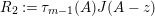
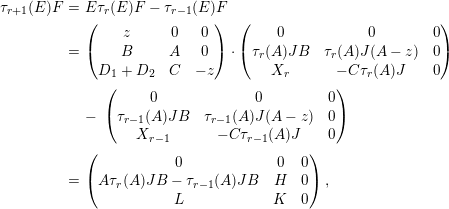 $$\begin{eqnarray}\displaystyle \unicode[STIX]{x1D70F}_{r+1}(E)F & = & \displaystyle E\unicode[STIX]{x1D70F}_{r}(E)F-\unicode[STIX]{x1D70F}_{r-1}(E)F\nonumber\\ \displaystyle & = & \displaystyle \left(\begin{array}{@{}ccc@{}}z & 0 & 0\\ B & A & 0\\ D_{1}+D_{2} & C & -z\end{array}\right)\cdot \left(\begin{array}{@{}ccc@{}}0 & 0 & 0\\ \unicode[STIX]{x1D70F}_{r}(A)JB & \unicode[STIX]{x1D70F}_{r}(A)J(A-z) & 0\\ X_{r} & -C\unicode[STIX]{x1D70F}_{r}(A)J & 0\end{array}\right)\nonumber\\ \displaystyle & & \displaystyle -\,\left(\begin{array}{@{}ccc@{}}0 & 0 & 0\\ \unicode[STIX]{x1D70F}_{r-1}(A)JB & \unicode[STIX]{x1D70F}_{r-1}(A)J(A-z) & 0\\ X_{r-1} & -C\unicode[STIX]{x1D70F}_{r-1}(A)J & 0\end{array}\right)\nonumber\\ \displaystyle & = & \displaystyle \left(\begin{array}{@{}ccc@{}}0 & 0 & 0\\ A\unicode[STIX]{x1D70F}_{r}(A)JB-\unicode[STIX]{x1D70F}_{r-1}(A)JB & H & 0\\ L & K & 0\end{array}\right),\nonumber\end{eqnarray}$$
where we use the abbreviations
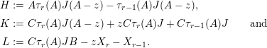 $$\begin{eqnarray}\displaystyle H & := & \displaystyle A\unicode[STIX]{x1D70F}_{r}(A)J(A-z)-\unicode[STIX]{x1D70F}_{r-1}(A)J(A-z),\nonumber\\ \displaystyle K & := & \displaystyle C\unicode[STIX]{x1D70F}_{r}(A)J(A-z)+zC\unicode[STIX]{x1D70F}_{r}(A)J+C\unicode[STIX]{x1D70F}_{r-1}(A)J\qquad \text{and}\nonumber\\ \displaystyle L & := & \displaystyle C\unicode[STIX]{x1D70F}_{r}(A)JB-zX_{r}-X_{r-1}.\nonumber\end{eqnarray}$$
At the positions
 $(2,1)$
and
$(2,1)$
and
 $(2,2)$
, the term is clearly equal to the desired result. At position
$(2,2)$
, the term is clearly equal to the desired result. At position
 $(3,2)$
, we use
$(3,2)$
, we use
 $JA=-AJ$
and simplify the expression as follows:
$JA=-AJ$
and simplify the expression as follows:
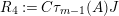
 $$\begin{eqnarray}\displaystyle K & = & \displaystyle C\unicode[STIX]{x1D70F}_{r}(A)JA-C\unicode[STIX]{x1D70F}_{r}(A)Jz+zC\unicode[STIX]{x1D70F}_{r}(A)J+C\unicode[STIX]{x1D70F}_{r-1}(A)J\nonumber\\ \displaystyle & = & \displaystyle -C\unicode[STIX]{x1D70F}_{r}(A)AJ+C\unicode[STIX]{x1D70F}_{r-1}(A)J\nonumber\\ \displaystyle & = & \displaystyle -C\unicode[STIX]{x1D70F}_{r+1}(A)J.\nonumber\end{eqnarray}$$
Using the recursive definition of
 $\unicode[STIX]{x1D70F}_{r+1}$
, it is also a routine calculation to show that
$\unicode[STIX]{x1D70F}_{r+1}$
, it is also a routine calculation to show that
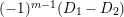
 $$\begin{eqnarray}L=\mathop{\sum }_{i=0}^{r}(-1)^{i}C\unicode[STIX]{x1D70F}_{i}(z)\unicode[STIX]{x1D70F}_{r-i}(A)JB+(-1)^{r+1}\unicode[STIX]{x1D70F}_{r+1}(z)(D_{1}-D_{2}).\end{eqnarray}$$
This shows (∗).
Step 2. Simplify the result
Now, let
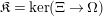 $\mathfrak{K}=\ker (\unicode[STIX]{x1D6EF}\rightarrow \unicode[STIX]{x1D6FA})$
. By definition, this ideal is generated by the coefficients of the
$\mathfrak{K}=\ker (\unicode[STIX]{x1D6EF}\rightarrow \unicode[STIX]{x1D6FA})$
. By definition, this ideal is generated by the coefficients of the
 $v^{\unicode[STIX]{x1D6FE}}$
in
$v^{\unicode[STIX]{x1D6FE}}$
in
 $\unicode[STIX]{x1D6E5}_{m}(\unicode[STIX]{x1D704}(T_{s}),\unicode[STIX]{x1D704}(T_{t}))\in \mathbb{Z}[v^{\pm 1}]\unicode[STIX]{x1D6EF}$
. Therefore, we consider the coefficients of
$\unicode[STIX]{x1D6E5}_{m}(\unicode[STIX]{x1D704}(T_{s}),\unicode[STIX]{x1D704}(T_{t}))\in \mathbb{Z}[v^{\pm 1}]\unicode[STIX]{x1D6EF}$
. Therefore, we consider the coefficients of
-
(1)
$R_{1}:=\unicode[STIX]{x1D70F}_{m-1}(A)JB$
, -
(2)
$R_{2}:=\unicode[STIX]{x1D70F}_{m-1}(A)J(A-z)$
, -
(3)
$R_{3}:=\sum _{i=0}^{m-2}(-1)^{i}C\unicode[STIX]{x1D70F}_{i}(z)\unicode[STIX]{x1D70F}_{m-2-i}(A)JB+(-1)^{m-1}\unicode[STIX]{x1D70F}_{m-1}(z)(D_{1}-D_{2})$
and -
(4)
$R_{4}:=C\unicode[STIX]{x1D70F}_{m-1}(A)J$
.

The coefficient of the highest power of
 $v$
in
$v$
in
 $R_{2}$
is
$R_{2}$
is
 $-\unicode[STIX]{x1D70F}_{m-1}(A)J$
because
$-\unicode[STIX]{x1D70F}_{m-1}(A)J$
because
 $z=v+v^{-1}$
, so that the coefficient of the highest power of
$z=v+v^{-1}$
, so that the coefficient of the highest power of
 $z$
is also the coefficient of the highest power of
$z$
is also the coefficient of the highest power of
 $v$
in any Laurent polynomial. Now,
$v$
in any Laurent polynomial. Now,
 $R_{2}$
is contained in
$R_{2}$
is contained in
 $\mathfrak{K}[v^{\pm 1}]$
(remember that we view these matrices as elements of
$\mathfrak{K}[v^{\pm 1}]$
(remember that we view these matrices as elements of
 $\mathbb{Z}[v^{\pm 1}]\unicode[STIX]{x1D6EF}$
, so that this makes sense) if and only if
$\mathbb{Z}[v^{\pm 1}]\unicode[STIX]{x1D6EF}$
, so that this makes sense) if and only if
 $\unicode[STIX]{x1D70F}_{m-1}(A)\in \mathfrak{K}$
, because
$\unicode[STIX]{x1D70F}_{m-1}(A)\in \mathfrak{K}$
, because
 $J$
is invertible. Conversely,
$J$
is invertible. Conversely,
 $R_{1}$
,
$R_{1}$
,
 $R_{2}$
and
$R_{2}$
and
 $R_{4}$
are in
$R_{4}$
are in
 $\mathfrak{K}[v^{\pm 1}]$
if
$\mathfrak{K}[v^{\pm 1}]$
if
 $\unicode[STIX]{x1D70F}_{m-1}(A)\in \mathfrak{K}$
holds.
$\unicode[STIX]{x1D70F}_{m-1}(A)\in \mathfrak{K}$
holds.
Let us have a closer look at
 $R_{3}$
: the polynomial
$R_{3}$
: the polynomial
 $\unicode[STIX]{x1D70F}_{r}$
has degree
$\unicode[STIX]{x1D70F}_{r}$
has degree
 $r$
. The coefficient of the highest power of
$r$
. The coefficient of the highest power of
 $v$
in
$v$
in
 $R_{3}$
equals
$R_{3}$
equals
 $(-1)^{m-1}(D_{1}-D_{2})$
. Therefore,
$(-1)^{m-1}(D_{1}-D_{2})$
. Therefore,
 $D_{1}-D_{2}\in \mathfrak{K}$
, and
$D_{1}-D_{2}\in \mathfrak{K}$
, and
 $R_{3}$
is in
$R_{3}$
is in
 $\mathfrak{K}[v^{\pm 1}]$
if and only if
$\mathfrak{K}[v^{\pm 1}]$
if and only if
 $D_{1}-D_{2}\in \mathfrak{K}$
and
$D_{1}-D_{2}\in \mathfrak{K}$
and
 $R_{3}^{\prime }=\sum _{i=0}^{m-2}(-1)^{i}C\unicode[STIX]{x1D70F}_{i}(z)\unicode[STIX]{x1D70F}_{r-2-i}(A)JB\in \mathfrak{K}[v^{\pm 1}]$
. Looking repeatedly at the coefficient of the highest power of
$R_{3}^{\prime }=\sum _{i=0}^{m-2}(-1)^{i}C\unicode[STIX]{x1D70F}_{i}(z)\unicode[STIX]{x1D70F}_{r-2-i}(A)JB\in \mathfrak{K}[v^{\pm 1}]$
. Looking repeatedly at the coefficient of the highest power of
 $v$
and shortening the term, we get that
$v$
and shortening the term, we get that
 $R_{3}^{\prime }$
is in
$R_{3}^{\prime }$
is in
 $\mathfrak{K}[v^{\pm 1}]$
if and only if
$\mathfrak{K}[v^{\pm 1}]$
if and only if
 $C\unicode[STIX]{x1D70F}_{0}(A)JB,C\unicode[STIX]{x1D70F}_{1}(A)JB,\ldots ,C\unicode[STIX]{x1D70F}_{m-2}(A)JB\in \mathfrak{K}$
. Because
$C\unicode[STIX]{x1D70F}_{0}(A)JB,C\unicode[STIX]{x1D70F}_{1}(A)JB,\ldots ,C\unicode[STIX]{x1D70F}_{m-2}(A)JB\in \mathfrak{K}$
. Because
 $\{\unicode[STIX]{x1D70F}_{0},\ldots ,\unicode[STIX]{x1D70F}_{m-2}\}$
is a
$\{\unicode[STIX]{x1D70F}_{0},\ldots ,\unicode[STIX]{x1D70F}_{m-2}\}$
is a
 $\mathbb{Z}$
-basis of
$\mathbb{Z}$
-basis of
 $\{f\in \mathbb{Z}[T]\mid \deg (f)\leqslant m-2\}$
, these terms are in
$\{f\in \mathbb{Z}[T]\mid \deg (f)\leqslant m-2\}$
, these terms are in
 $\mathfrak{K}$
if and only if
$\mathfrak{K}$
if and only if
 $CA^{0}JB,CA^{1}JB,\ldots ,CA^{m-2}JB$
are.
$CA^{0}JB,CA^{1}JB,\ldots ,CA^{m-2}JB$
are.
Thus, we obtain the generating set
 $(\unicode[STIX]{x1D6FC})$
 $R_{\unicode[STIX]{x1D6FC}}:=\unicode[STIX]{x1D70F}_{m-1}(A)$
,
$R_{\unicode[STIX]{x1D6FC}}:=\unicode[STIX]{x1D70F}_{m-1}(A)$
,
 $(\unicode[STIX]{x1D6FD})$
 $R_{\unicode[STIX]{x1D6FD}}:=D_{1}-D_{2}$
and
$R_{\unicode[STIX]{x1D6FD}}:=D_{1}-D_{2}$
and
 $(\unicode[STIX]{x1D6FE})$
 $R_{\unicode[STIX]{x1D6FE},k}:=CA^{k}JB$
for
$R_{\unicode[STIX]{x1D6FE},k}:=CA^{k}JB$
for
 $0\leqslant k\leqslant m-2$
,
$0\leqslant k\leqslant m-2$
,
for the ideal
 $\mathfrak{K}$
.
$\mathfrak{K}$
.
Step 3. The relations.
Again, we decompose
 $\unicode[STIX]{x1D6EF}$
as
$\unicode[STIX]{x1D6EF}$
as
 $\bigoplus _{I}\unicode[STIX]{x1D6EF}E_{I}$
and use
$\bigoplus _{I}\unicode[STIX]{x1D6EF}E_{I}$
and use
 $R\in \mathfrak{K}$
if and only if
$R\in \mathfrak{K}$
if and only if
 $E_{I}RE_{J}$
in
$E_{I}RE_{J}$
in
 $\mathfrak{K}$
for all
$\mathfrak{K}$
for all
 $I,J\subseteq S$
.
$I,J\subseteq S$
.
To determine
 $E_{I}R_{\unicode[STIX]{x1D6FC}}E_{J}$
, we consider
$E_{I}R_{\unicode[STIX]{x1D6FC}}E_{J}$
, we consider
 $E_{I}A^{k}E_{J}$
. For
$E_{I}A^{k}E_{J}$
. For
 $k=0$
, this simplifies to
$k=0$
, this simplifies to
 $E_{I}A^{0}E_{J}=\unicode[STIX]{x1D6FF}_{\mathit{IJ}}E_{I}=P_{\mathit{IJ}}^{0}$
. For
$E_{I}A^{0}E_{J}=\unicode[STIX]{x1D6FF}_{\mathit{IJ}}E_{I}=P_{\mathit{IJ}}^{0}$
. For
 $k>0$
, we obtain
$k>0$
, we obtain
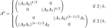 $$\begin{eqnarray}A^{k}=\left\{\begin{array}{@{}ll@{}}\left(\begin{array}{@{}cc@{}}(A_{1}A_{2})^{k/2} & 0\\ 0 & (A_{2}A_{1})^{k/2}\end{array}\right)\quad & \text{if}~2\mid k,\\ \left(\begin{array}{@{}cc@{}}0 & (A_{1}A_{2})^{(k-1)/2}A_{1}\\ (A_{2}A_{1})^{(k-1)/2}A_{2} & 0\end{array}\right)\quad & \text{if}~2\nmid k,\end{array}\right.\end{eqnarray}$$
and substitute
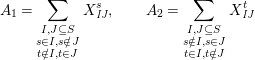 $$\begin{eqnarray}A_{1}=\mathop{\sum }_{\substack{ I,J\subseteq S \\ s\in I,s\notin J \\ t\notin I,t\in J}}X_{\mathit{IJ}}^{s},\qquad A_{2}=\mathop{\sum }_{\substack{ I,J\subseteq S \\ s\notin I,s\in J \\ t\in I,t\notin J}}X_{\mathit{IJ}}^{t}\end{eqnarray}$$
to obtain
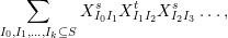 $$\begin{eqnarray}\mathop{\sum }_{I_{0},I_{1},\ldots ,I_{k}\subseteq S}X_{I_{0}I_{1}}^{s}X_{I_{1}I_{2}}^{t}X_{I_{2}I_{3}}^{s}\ldots ,\end{eqnarray}$$
where the sum is over all
 $I_{i}$
that satisfy
$I_{i}$
that satisfy
 $s\in I_{2i}\setminus I_{2i+1}$
and
$s\in I_{2i}\setminus I_{2i+1}$
and
 $t\in I_{2i+1}\setminus I_{2i}$
when we consider
$t\in I_{2i+1}\setminus I_{2i}$
when we consider
 $A_{1}A_{2}A_{1}\ldots$
. Because
$A_{1}A_{2}A_{1}\ldots$
. Because
 $X_{\mathit{IJ}}^{s}=0$
if
$X_{\mathit{IJ}}^{s}=0$
if
 $s\notin I\setminus J$
, only the conditions for
$s\notin I\setminus J$
, only the conditions for
 $I=I_{0}$
and
$I=I_{0}$
and
 $I_{k}=J$
are not vacuous. Therefore, we could just sum over all paths of length
$I_{k}=J$
are not vacuous. Therefore, we could just sum over all paths of length
 $k$
that go to
$k$
that go to
 $I$
from
$I$
from
 $J$
. We therefore obtain
$J$
. We therefore obtain
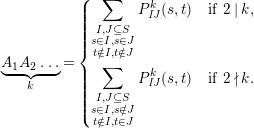 $$\begin{eqnarray}\underbrace{A_{1}A_{2}\ldots }_{k}=\left\{\begin{array}{@{}ll@{}}\displaystyle \mathop{\sum }_{\substack{ I,J\subseteq S \\ s\in I,s\in J \\ t\notin I,t\notin J}}P_{\mathit{IJ}}^{k}(s,t)\quad & \text{if}~2\mid k,\\ \displaystyle \mathop{\sum }_{\substack{ I,J\subseteq S \\ s\in I,s\notin J \\ t\notin I,t\in J}}P_{\mathit{IJ}}^{k}(s,t)\quad & \text{if}~2\nmid k.\end{array}\right.\end{eqnarray}$$
For the other product, we similarly obtain
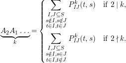 $$\begin{eqnarray}\underbrace{A_{2}A_{1}\ldots }_{k}=\left\{\begin{array}{@{}ll@{}}\displaystyle \mathop{\sum }_{\substack{ I,J\subseteq S \\ s\notin I,s\notin J \\ t\in I,t\in J}}P_{\mathit{IJ}}^{k}(t,s)\quad & \text{if}~2\mid k,\\ \displaystyle \mathop{\sum }_{\substack{ I,J\subseteq S \\ s\notin I,s\in J \\ t\in I,t\notin J}}P_{\mathit{IJ}}^{k}(t,s)\quad & \text{if}~2\nmid k.\end{array}\right.\end{eqnarray}$$
Multiplying with
 $E_{I}$
from the left and with
$E_{I}$
from the left and with
 $E_{J}$
from the right, this equals either
$E_{J}$
from the right, this equals either
 $0$
or
$0$
or
 $P_{\mathit{IJ}}^{k}(s,t)$
and
$P_{\mathit{IJ}}^{k}(s,t)$
and
 $P_{\mathit{IJ}}^{k}(t,s)$
, respectively. The element
$P_{\mathit{IJ}}^{k}(t,s)$
, respectively. The element
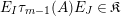 $E_{I}\unicode[STIX]{x1D70F}_{m-1}(A)E_{J}\in \mathfrak{K}$
is, if it is not zero, equal to
$E_{I}\unicode[STIX]{x1D70F}_{m-1}(A)E_{J}\in \mathfrak{K}$
is, if it is not zero, equal to
 $$\begin{eqnarray}P_{\mathit{IJ}}^{m-1}(s,t)+a_{m-2}P_{\mathit{IJ}}^{m-2}(s,t)+\cdots +a_{2}P_{\mathit{IJ}}^{2}(s,t)+a_{1}P_{\mathit{IJ}}^{1}(s,t)+a_{0}P_{\mathit{IJ}}^{0}(s,t),\end{eqnarray}$$
where
 $\unicode[STIX]{x1D70F}_{m-1}(T)=T^{m-1}+a_{m-2}T^{m-2}+\cdots +a_{2}T^{2}+a_{1}T^{1}+a_{0}$
, and similarly for the symmetric situation where
$\unicode[STIX]{x1D70F}_{m-1}(T)=T^{m-1}+a_{m-2}T^{m-2}+\cdots +a_{2}T^{2}+a_{1}T^{1}+a_{0}$
, and similarly for the symmetric situation where
 $s,t$
are swapped.
$s,t$
are swapped.
The second kind of generator is easier:
 $R_{\unicode[STIX]{x1D6FD}}$
is equal to
$R_{\unicode[STIX]{x1D6FD}}$
is equal to
 $$\begin{eqnarray}\mathop{\sum }_{\substack{ I,J\subseteq S \\ s\in I,s\notin J \\ t\in I,t\notin J}}X_{\mathit{IJ}}^{s}-X_{\mathit{IJ}}^{t}.\end{eqnarray}$$
For those
 $I$
,
$I$
,
 $J$
that do not occur in this sum,
$J$
that do not occur in this sum,
 $E_{I}R_{\unicode[STIX]{x1D6FD}}E_{J}=0$
. For all others, we obtain the element
$E_{I}R_{\unicode[STIX]{x1D6FD}}E_{J}=0$
. For all others, we obtain the element
 $X_{\mathit{IJ}}^{s}-X_{\mathit{IJ}}^{t}=P_{\mathit{IJ}}^{1}(s,t)-P_{\mathit{IJ}}^{1}(t,s)$
. This is the first case in the relations of type
$X_{\mathit{IJ}}^{s}-X_{\mathit{IJ}}^{t}=P_{\mathit{IJ}}^{1}(s,t)-P_{\mathit{IJ}}^{1}(t,s)$
. This is the first case in the relations of type
 $(\unicode[STIX]{x1D6FD})$
.
$(\unicode[STIX]{x1D6FD})$
.
Finally, there is only one kind of generator left, namely
 $R_{\unicode[STIX]{x1D6FE},k}=CA^{k}JB$
. We already know the powers of
$R_{\unicode[STIX]{x1D6FE},k}=CA^{k}JB$
. We already know the powers of
 $A$
, and therefore obtain
$A$
, and therefore obtain
 $$\begin{eqnarray}CA^{k}JB=\left\{\begin{array}{@{}ll@{}}C_{2}(A_{1}A_{2})^{k/2}B_{1}-C_{1}(A_{2}A_{1})^{k/2}B_{2}\quad & \text{if}~2\mid k,\\ -C_{2}(A_{1}A_{2})^{(k-1)/2}A_{1}B_{2}+C_{1}(A_{2}A_{1})^{(k-1)/2}A_{2}B_{1}\quad & \text{if}~2\nmid k.\end{array}\right.\end{eqnarray}$$
We substitute the definitions
 $$\begin{eqnarray}\displaystyle & \displaystyle B_{1}=\mathop{\sum }_{\substack{ I,J\subseteq S \\ s\in I,s\notin J \\ t\notin I,t\notin J}}X_{\mathit{IJ}}^{s},\qquad B_{2}=\mathop{\sum }_{\substack{ I,J\subseteq S \\ s\notin I,s\notin J \\ t\in I,t\notin J}}X_{\mathit{IJ}}^{t}, & \displaystyle \nonumber\\ \displaystyle & \displaystyle C_{1}=\mathop{\sum }_{\substack{ I,J\subseteq S \\ s\in I,s\notin J \\ t\in I,t\in J}}X_{\mathit{IJ}}^{s},\qquad C_{2}=\mathop{\sum }_{\substack{ I,J\subseteq S \\ s\in I,s\in J \\ t\in I,t\notin J}}X_{\mathit{IJ}}^{t}. & \displaystyle \nonumber\end{eqnarray}$$
If
 $s,t\in I$
or
$s,t\in I$
or
 $s,t\notin J$
is not satisfied, then
$s,t\notin J$
is not satisfied, then
 $E_{I}CA^{k}JBE_{J}=0$
, because either
$E_{I}CA^{k}JBE_{J}=0$
, because either
 $E_{I}C=0$
or
$E_{I}C=0$
or
 $BE_{J}=0$
. Otherwise,
$BE_{J}=0$
. Otherwise,
 $$\begin{eqnarray}\displaystyle E_{I}CA^{k}JBE_{J} & = & \displaystyle \mathop{\sum }_{I_{0},\ldots ,I_{k}\subseteq S}X_{II_{0}}^{t}X_{I_{0}I_{1}}^{s}\ldots X_{I_{k-1}I_{k}}^{t}X_{I_{k}J}^{s}\nonumber\\ \displaystyle & & \displaystyle -\,X_{I,I_{0}}^{s}X_{I_{0}I_{1}}^{t}\ldots X_{I_{k-1}I_{k}}^{s}X_{I_{k}J}^{t}\nonumber\\ \displaystyle & = & \displaystyle P_{\mathit{IJ}}^{k+2}(t,s)-P_{\mathit{IJ}}^{k+2}(s,t)\nonumber\end{eqnarray}$$
holds if
 $2\mid k$
and
$2\mid k$
and
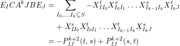 $$\begin{eqnarray}\displaystyle E_{I}CA^{k}JBE_{J} & = & \displaystyle \mathop{\sum }_{I_{0},\ldots ,I_{k}\subseteq S}-X_{II_{0}}^{t}X_{I_{0}I_{1}}^{s}\ldots X_{I_{k-1}I_{k}}^{s}X_{I_{k}J}^{t}\nonumber\\ \displaystyle & & \displaystyle +\,X_{II_{0}}^{s}X_{I_{0}I_{1}}^{t}\ldots X_{I_{k-1}I_{k}}^{t}X_{I_{k}J}^{s}\nonumber\\ \displaystyle & = & \displaystyle -P_{\mathit{IJ}}^{k+2}(t,s)+P_{\mathit{IJ}}^{k+2}(s,t)\nonumber\end{eqnarray}$$
holds if
 $2\nmid k$
. This provides the other elements in the relations of type
$2\nmid k$
. This provides the other elements in the relations of type
 $(\unicode[STIX]{x1D6FD})$
.◻
$(\unicode[STIX]{x1D6FD})$
.◻
Because of the
 $(\unicode[STIX]{x1D6FD})$
-relation
$(\unicode[STIX]{x1D6FD})$
-relation
 $X_{\mathit{IJ}}^{s}-X_{\mathit{IJ}}^{t}=P_{\mathit{IJ}}^{1}(s,t)-P_{\mathit{IJ}}^{1}(t,s)=0$
in
$X_{\mathit{IJ}}^{s}-X_{\mathit{IJ}}^{t}=P_{\mathit{IJ}}^{1}(s,t)-P_{\mathit{IJ}}^{1}(t,s)=0$
in
 $\unicode[STIX]{x1D6FA}$
, the upper index of these elements does not matter, and it is well defined to write
$\unicode[STIX]{x1D6FA}$
, the upper index of these elements does not matter, and it is well defined to write
 $X_{\mathit{IJ}}$
for the common value of
$X_{\mathit{IJ}}$
for the common value of
 $X_{\mathit{IJ}}^{s}\in \unicode[STIX]{x1D6FA}$
for all
$X_{\mathit{IJ}}^{s}\in \unicode[STIX]{x1D6FA}$
for all
 $s\in I\setminus J$
. We adopt this notation for the rest of this article.
$s\in I\setminus J$
. We adopt this notation for the rest of this article.
Additionally,
 $(\unicode[STIX]{x1D6FC})$
implies that
$(\unicode[STIX]{x1D6FC})$
implies that
 $X_{\mathit{IJ}}^{s}=X_{\mathit{JI}}^{t}=0$
holds in
$X_{\mathit{IJ}}^{s}=X_{\mathit{JI}}^{t}=0$
holds in
 $\unicode[STIX]{x1D6FA}$
for all
$\unicode[STIX]{x1D6FA}$
for all
 $I,J\subseteq S$
,
$I,J\subseteq S$
,
 $s\in I\setminus J$
,
$s\in I\setminus J$
,
 $t\in J\setminus I$
with
$t\in J\setminus I$
with
 $m_{st}=2$
(i.e.,
$m_{st}=2$
(i.e.,
 $s$
and
$s$
and
 $t$
are not connected in the Dynkin diagram of
$t$
are not connected in the Dynkin diagram of
 $(W,S)$
). This allows us to think of
$(W,S)$
). This allows us to think of
 $\unicode[STIX]{x1D6FA}$
as a quotient of a path algebra over a much simpler quiver, which was defined by Stembridge [Reference Stembridge8, Section 4].
$\unicode[STIX]{x1D6FA}$
as a quotient of a path algebra over a much simpler quiver, which was defined by Stembridge [Reference Stembridge8, Section 4].
Definition 14. The compatibility graph of
 $(W,S)$
is the directed graph
$(W,S)$
is the directed graph
 ${\mathcal{Q}}_{W}$
with vertex set
${\mathcal{Q}}_{W}$
with vertex set
 $\{I\mid I\subseteq S\}$
and a single edge
$\{I\mid I\subseteq S\}$
and a single edge
 $I\leftarrow J$
if and only if
$I\leftarrow J$
if and only if
 $I\setminus J\neq \emptyset$
and no element of
$I\setminus J\neq \emptyset$
and no element of
 $I\setminus J$
commutes with any element of
$I\setminus J$
commutes with any element of
 $J\setminus I$
.
$J\setminus I$
.
An edge
 $I\leftarrow J$
with
$I\leftarrow J$
with
 $I\supseteq J$
is called an inclusion edge; all other edges are called transversal edges.
$I\supseteq J$
is called an inclusion edge; all other edges are called transversal edges.
Note that transversal edges always occur in pairs of opposite orientation because their definition is symmetric:
 $I\leftarrow J$
is a transversal edge if and only if
$I\leftarrow J$
is a transversal edge if and only if
 $I\setminus J\neq \emptyset$
,
$I\setminus J\neq \emptyset$
,
 $J\setminus I\neq \emptyset$
and all
$J\setminus I\neq \emptyset$
and all
 $s\in I\setminus J$
are connected to all
$s\in I\setminus J$
are connected to all
 $t\in J\setminus I$
in the Dynkin diagram of
$t\in J\setminus I$
in the Dynkin diagram of
 $(W,S)$
.
$(W,S)$
.
Corollary 15.
 $\unicode[STIX]{x1D6FA}$
is a quotient of the path algebra
$\unicode[STIX]{x1D6FA}$
is a quotient of the path algebra
 $\mathbb{Z}{\mathcal{Q}}_{W}$
.
$\mathbb{Z}{\mathcal{Q}}_{W}$
.
Proof. Denote the vertex elements in
 $\mathbb{Z}{\mathcal{Q}}_{W}$
by
$\mathbb{Z}{\mathcal{Q}}_{W}$
by
 $\tilde{E}_{I}$
and the edge elements by
$\tilde{E}_{I}$
and the edge elements by
 $\tilde{X}_{\mathit{IJ}}$
. Then,
$\tilde{X}_{\mathit{IJ}}$
. Then,
 $\tilde{E}_{I}\mapsto E_{I}$
and
$\tilde{E}_{I}\mapsto E_{I}$
and
 $\tilde{X}_{\mathit{IJ}}\mapsto X_{\mathit{IJ}}^{s}$
with any
$\tilde{X}_{\mathit{IJ}}\mapsto X_{\mathit{IJ}}^{s}$
with any
 $s\in I\setminus J$
extends to a well-defined algebra homomorphism
$s\in I\setminus J$
extends to a well-defined algebra homomorphism
 $\mathbb{Z}{\mathcal{Q}}_{W}\rightarrow \unicode[STIX]{x1D6FA}$
by the
$\mathbb{Z}{\mathcal{Q}}_{W}\rightarrow \unicode[STIX]{x1D6FA}$
by the
 $(\unicode[STIX]{x1D6FD})$
-relation. It is surjective because all elements
$(\unicode[STIX]{x1D6FD})$
-relation. It is surjective because all elements
 $X_{\mathit{IJ}}^{s}\in \unicode[STIX]{x1D6FA}$
are either zero by some
$X_{\mathit{IJ}}^{s}\in \unicode[STIX]{x1D6FA}$
are either zero by some
 $(\unicode[STIX]{x1D6FC})$
-type relation as seen above or contained in the image of this morphism, and
$(\unicode[STIX]{x1D6FC})$
-type relation as seen above or contained in the image of this morphism, and
 $\unicode[STIX]{x1D6FA}$
is generated by the elements
$\unicode[STIX]{x1D6FA}$
is generated by the elements
 $X_{\mathit{IJ}}^{s}$
and
$X_{\mathit{IJ}}^{s}$
and
 $E_{I}$
.◻
$E_{I}$
.◻
Example 16. Figure 1 displays the compatibility graphs of the finite irreducible Coxeter groups of rank
 ${\leqslant}4$
. For the sake of clarity, inclusion edges are only displayed in rank 2 and rank 3 and only between those
${\leqslant}4$
. For the sake of clarity, inclusion edges are only displayed in rank 2 and rank 3 and only between those
 $I,J\subseteq S$
that satisfy
$I,J\subseteq S$
that satisfy
 $\left|I\setminus J\right|=1$
. Pairs of transversal edges
$\left|I\setminus J\right|=1$
. Pairs of transversal edges
 $I\leftrightarrows J$
are combined into one (bold) undirected edge.
$I\leftrightarrows J$
are combined into one (bold) undirected edge.
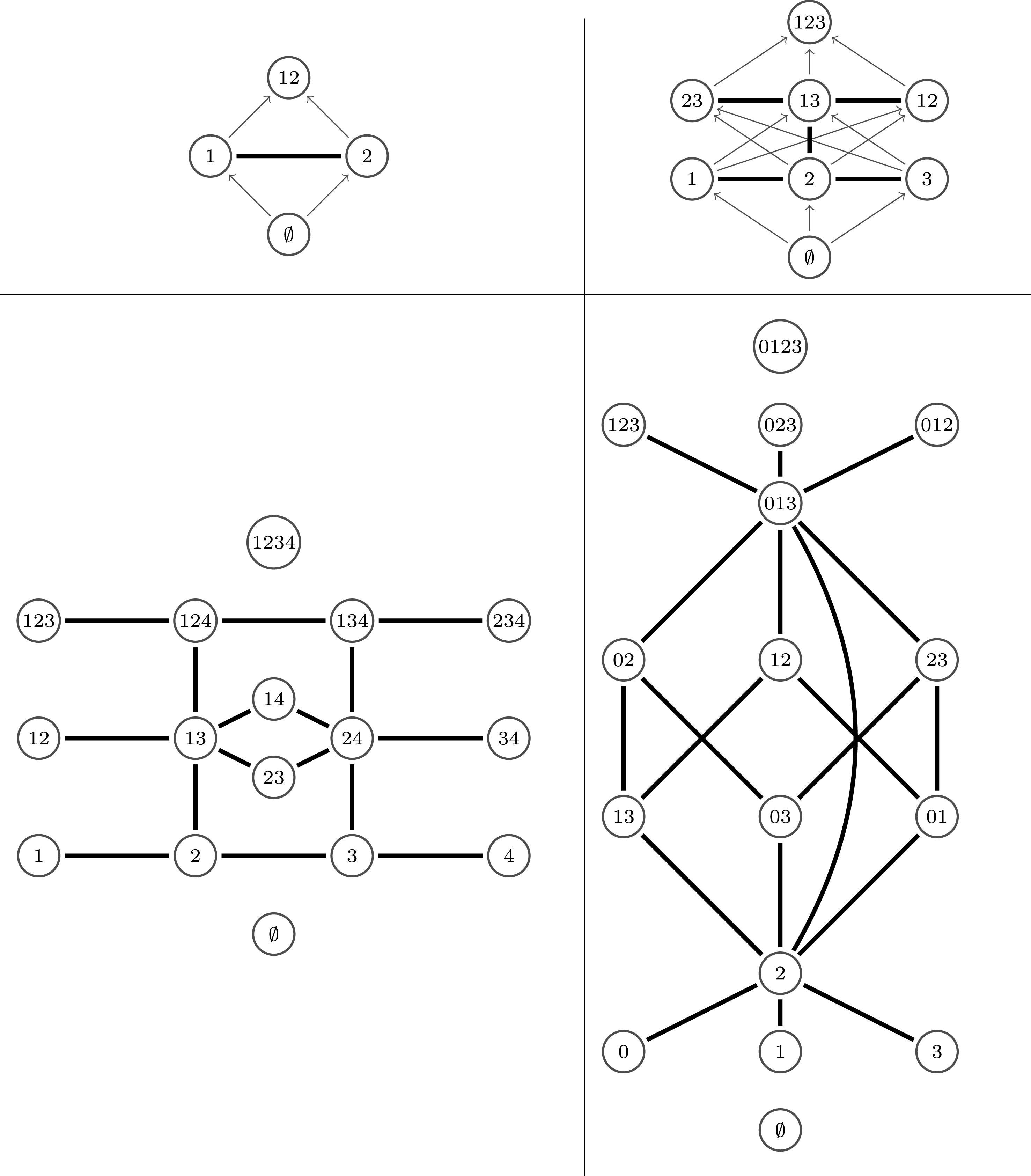
Figure 1. Compatibility graphs for small Coxeter groups: top left for
 $I_{2}(m)$
; top right for
$I_{2}(m)$
; top right for
 $A_{3}$
,
$A_{3}$
,
 $B_{3}$
and
$B_{3}$
and
 $H_{3}$
; bottom left for
$H_{3}$
; bottom left for
 $A_{4}$
,
$A_{4}$
,
 $B_{4}$
and
$B_{4}$
and
 $F_{4}$
; bottom right for
$F_{4}$
; bottom right for
 $D_{4}$
.
$D_{4}$
.
4 The decomposition conjecture
While trying to prove Gyoja’s conjectureFootnote
1
and to better understand the internal structure of
 $\unicode[STIX]{x1D6FA}$
and
$\unicode[STIX]{x1D6FA}$
and
 $W$
-graphs, I found a number of very similar proofs for some small types of Coxeter groups. The essence of these proofs is captured by the following four conjectural properties of
$W$
-graphs, I found a number of very similar proofs for some small types of Coxeter groups. The essence of these proofs is captured by the following four conjectural properties of
 $\unicode[STIX]{x1D6FA}$
.
$\unicode[STIX]{x1D6FA}$
.
Conjecture 17. Let
 $k\subseteq \mathbb{C}$
be a good ring for
$k\subseteq \mathbb{C}$
be a good ring for
 $(W,S)$
. There exists a family
$(W,S)$
. There exists a family
 $(F^{\unicode[STIX]{x1D706}})_{\unicode[STIX]{x1D706}\in \text{Irr}(W)}$
of elements of
$(F^{\unicode[STIX]{x1D706}})_{\unicode[STIX]{x1D706}\in \text{Irr}(W)}$
of elements of
 $k\unicode[STIX]{x1D6FA}$
with the following properties.
$k\unicode[STIX]{x1D6FA}$
with the following properties.
-
(Z1) The
$F^{\unicode[STIX]{x1D706}}$
are pairwise orthogonal idempotents and decompose the identity
$$\begin{eqnarray}\forall \unicode[STIX]{x1D706},\unicode[STIX]{x1D707}\in \text{Irr}(W):F^{\unicode[STIX]{x1D706}}F^{\unicode[STIX]{x1D707}}=\unicode[STIX]{x1D6FF}_{\unicode[STIX]{x1D706}\unicode[STIX]{x1D707}}F^{\unicode[STIX]{x1D706}},\qquad 1=\mathop{\sum }_{\unicode[STIX]{x1D706}\in \text{Irr}(W)}F^{\unicode[STIX]{x1D706}}.\end{eqnarray}$$
-
(Z2) This decomposition is compatible with the decomposition induced by the path-algebra structure:
$$\begin{eqnarray}\forall \unicode[STIX]{x1D706}\in \text{Irr}(W)\forall I\subseteq S:E_{I}F^{\unicode[STIX]{x1D706}}=F^{\unicode[STIX]{x1D706}}E_{I}.\end{eqnarray}$$
-
(Z3) There is a partial order
$\preccurlyeq$
on
$\text{Irr}(W)$
such that only downward edges exist: if
$F^{\unicode[STIX]{x1D706}}k\unicode[STIX]{x1D6FA}F^{\unicode[STIX]{x1D707}}\neq 0$
, then
$\unicode[STIX]{x1D706}\preccurlyeq \unicode[STIX]{x1D707}$
. -
(Z4) There are surjective
$k$
-algebra morphisms
$\unicode[STIX]{x1D713}_{\unicode[STIX]{x1D706}}:k^{d_{\unicode[STIX]{x1D706}}\times d_{\unicode[STIX]{x1D706}}}{\twoheadrightarrow}F^{\unicode[STIX]{x1D706}}k\unicode[STIX]{x1D6FA}F^{\unicode[STIX]{x1D706}}$
for all
$\unicode[STIX]{x1D706}\in \text{Irr}(W)$
, where
$d_{\unicode[STIX]{x1D706}}$
denotes the degree of the character
$\unicode[STIX]{x1D706}$
.

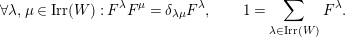


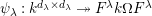


Remark 18. The edge terminology in (Z3) refers to the quiver
 $\unicode[STIX]{x1D6EC}$
in the next theorem.
$\unicode[STIX]{x1D6EC}$
in the next theorem.
The decomposition conjecture is of interest because it implies several important properties of the
 $W$
-graph algebra and its modules (that is,
$W$
-graph algebra and its modules (that is,
 $W$
-graphs), as the following theorem demonstrates.
$W$
-graphs), as the following theorem demonstrates.
Theorem 19. Assume that the decomposition conjecture is true for the finite Coxeter group
 $(W,S)$
and
$(W,S)$
and
 $k$
a good ring for
$k$
a good ring for
 $(W,S)$
. Then, the following properties hold.
$(W,S)$
. Then, the following properties hold.
-
(1) Consider the quiver
$\unicode[STIX]{x1D6EC}$
which has
$\text{Irr}(W)$
as its set of vertices and an edge
$\unicode[STIX]{x1D706}\leftarrow \unicode[STIX]{x1D707}$
if and only if
$\unicode[STIX]{x1D706}\prec \unicode[STIX]{x1D707}$
. Then,
$k\unicode[STIX]{x1D6FA}$
is a quotient of the generalized path algebra (cf. [Reference Coelho and Liu2]) over the quiver
$\unicode[STIX]{x1D6EC}$
which has
$k^{d_{\unicode[STIX]{x1D706}}\times d_{\unicode[STIX]{x1D706}}}$
as vertex algebras. -
(2)
$k\unicode[STIX]{x1D6FA}$
is finitely generated as a
$k$
-module.


Furthermore, if
 $k$
is a field then the following hold:
$k$
is a field then the following hold:
-
(3) The Jacobson radical
$\text{rad}(k\unicode[STIX]{x1D6FA})$
is generated by the elements
$F^{\unicode[STIX]{x1D706}}X_{\mathit{IJ}}F^{\unicode[STIX]{x1D707}}$
with
$\unicode[STIX]{x1D706}\prec \unicode[STIX]{x1D707}$
and
$k\unicode[STIX]{x1D6FA}/\text{rad}(k\unicode[STIX]{x1D6FA})\cong \prod _{\unicode[STIX]{x1D706}\in \text{Irr}(W)}k^{d_{\unicode[STIX]{x1D706}}\times d_{\unicode[STIX]{x1D706}}}$
.


-
(4) A
$k\unicode[STIX]{x1D6FA}$
-module
$V$
is simple if and only if the restriction of
$k(v)V$
to
$k(v)H$
is simple. Furthermore (after reindexing the family
$(F^{\unicode[STIX]{x1D706}})_{\unicode[STIX]{x1D706}\in \text{Irr}(W)}$
if necessary), the latter has isomorphism class
$\unicode[STIX]{x1D706}$
if and only if
$F^{\unicode[STIX]{x1D706}}V=V$
holds.


-
(5) Every
$k\unicode[STIX]{x1D6FA}$
-module
$V$
has a family of natural submodules
$(V^{\preccurlyeq \unicode[STIX]{x1D706}})_{\unicode[STIX]{x1D706}\in \text{Irr}(W)}$
such that-
∙
$\unicode[STIX]{x1D706}\preccurlyeq \unicode[STIX]{x1D707}\;\Longrightarrow \;V^{\preccurlyeq \unicode[STIX]{x1D706}}\leqslant V^{\preccurlyeq \unicode[STIX]{x1D707}}$
and -
∙
$V^{\preccurlyeq \unicode[STIX]{x1D706}}/V^{\prec \unicode[STIX]{x1D706}}$
is isomorphic to a direct sum of irreducibles of isomorphism class
$\unicode[STIX]{x1D706}$
, where
$V^{\prec \unicode[STIX]{x1D706}}:=\sum _{\unicode[STIX]{x1D707}\prec \unicode[STIX]{x1D706}}V^{\preccurlyeq \unicode[STIX]{x1D707}}$
.
-


Remark 20. Given that the Kazhdan–Lusztig-
 $W$
-graph is indecomposable but not irreducible, it cannot be expected that an arbitrary
$W$
-graph is indecomposable but not irreducible, it cannot be expected that an arbitrary
 $\unicode[STIX]{x1D6FA}$
-module decomposes as a direct sum of its irreducible constituents. The special filtration appearing in the above theorem is the next best thing one can hope for: one finds the irreducible constituents in the layers of a natural filtration, and even nicely grouped into isomorphism classes. This fact and the first part of the theorem, saying that
$\unicode[STIX]{x1D6FA}$
-module decomposes as a direct sum of its irreducible constituents. The special filtration appearing in the above theorem is the next best thing one can hope for: one finds the irreducible constituents in the layers of a natural filtration, and even nicely grouped into isomorphism classes. This fact and the first part of the theorem, saying that
 $\unicode[STIX]{x1D6FA}$
itself is composed of much simpler parts like matrix algebras and path algebras, motivates the name decomposition conjecture.
$\unicode[STIX]{x1D6FA}$
itself is composed of much simpler parts like matrix algebras and path algebras, motivates the name decomposition conjecture.
To the best of my knowledge, the decomposition conjecture has neither directly nor in a similar form been stated before in the literature, apart from my dissertation [Reference Hahn5]. The above consequences of Conjecture 17 also have not been considered or proved before, even in special cases, as far as I know.
Proof. Denote with
 $k\widetilde{\unicode[STIX]{x1D6FA}}$
this generalized path algebra, and recall that it is characterized by the following properties:
$k\widetilde{\unicode[STIX]{x1D6FA}}$
this generalized path algebra, and recall that it is characterized by the following properties:
-
∙ it contains a set of pairwise orthogonal idempotents
$f_{\unicode[STIX]{x1D706}}$
corresponding to the vertices such that
$\sum _{\unicode[STIX]{x1D706}}f_{\unicode[STIX]{x1D706}}=1$
and
$f_{\unicode[STIX]{x1D706}}k\widetilde{\unicode[STIX]{x1D6FA}}f_{\unicode[STIX]{x1D706}}=k^{d_{\unicode[STIX]{x1D706}}\times d_{\unicode[STIX]{x1D706}}}$
; -
∙ it contains a set of elements
$y_{\unicode[STIX]{x1D706}\unicode[STIX]{x1D707}}$
corresponding to the edges
$\unicode[STIX]{x1D706}\leftarrow \unicode[STIX]{x1D707}$
such that
$y_{\unicode[STIX]{x1D706}\unicode[STIX]{x1D707}}=f_{\unicode[STIX]{x1D706}}y_{\unicode[STIX]{x1D706}\unicode[STIX]{x1D707}}f_{\unicode[STIX]{x1D707}}$
; -
∙ it satisfies the universal mapping property with respect to these features: for any
$k$
-algebra
$A$
, any set of elements
$\{f_{\unicode[STIX]{x1D706}}^{\prime },y_{\unicode[STIX]{x1D706}\unicode[STIX]{x1D707}}^{\prime }|\unicode[STIX]{x1D706},\unicode[STIX]{x1D707}\in \text{Irr}(W)\}$
satisfying these properties and any
$\unicode[STIX]{x1D713}_{\unicode[STIX]{x1D706}}:k^{d_{\unicode[STIX]{x1D706}}\times d_{\unicode[STIX]{x1D706}}}\rightarrow f_{\unicode[STIX]{x1D706}}^{\prime }Af_{\unicode[STIX]{x1D706}}^{\prime }$
, there exists a unique morphism of
$k$
-algebras
$\unicode[STIX]{x1D713}:k\widetilde{\unicode[STIX]{x1D6FA}}\rightarrow A$
with
$\unicode[STIX]{x1D713}(f_{\unicode[STIX]{x1D706}})=f_{\unicode[STIX]{x1D706}}^{\prime },\unicode[STIX]{x1D713}(y_{\unicode[STIX]{x1D706}\unicode[STIX]{x1D707}})=y_{\unicode[STIX]{x1D706}\unicode[STIX]{x1D707}}^{\prime }$
and
$\unicode[STIX]{x1D713}|f_{\unicode[STIX]{x1D706}}Af_{\unicode[STIX]{x1D706}}=\unicode[STIX]{x1D713}_{\unicode[STIX]{x1D706}}$
.


We define elements
 $Y_{\unicode[STIX]{x1D706}\unicode[STIX]{x1D707}}:=\sum _{I,J\subseteq S}F^{\unicode[STIX]{x1D706}}X_{\mathit{IJ}}F^{\unicode[STIX]{x1D707}}\in k\unicode[STIX]{x1D6FA}$
. Note that
$Y_{\unicode[STIX]{x1D706}\unicode[STIX]{x1D707}}:=\sum _{I,J\subseteq S}F^{\unicode[STIX]{x1D706}}X_{\mathit{IJ}}F^{\unicode[STIX]{x1D707}}\in k\unicode[STIX]{x1D6FA}$
. Note that
 $Y_{\unicode[STIX]{x1D706}\unicode[STIX]{x1D707}}=0$
if
$Y_{\unicode[STIX]{x1D706}\unicode[STIX]{x1D707}}=0$
if
 $\unicode[STIX]{x1D706}\not \preccurlyeq \unicode[STIX]{x1D707}$
, by (Z3). The universal property ensures that the morphisms from (Z4)
$\unicode[STIX]{x1D706}\not \preccurlyeq \unicode[STIX]{x1D707}$
, by (Z3). The universal property ensures that the morphisms from (Z4)
 $\unicode[STIX]{x1D713}_{\unicode[STIX]{x1D706}}:k^{d_{\unicode[STIX]{x1D706}}\times d_{\unicode[STIX]{x1D706}}}\rightarrow k\unicode[STIX]{x1D6FA}$
together with
$\unicode[STIX]{x1D713}_{\unicode[STIX]{x1D706}}:k^{d_{\unicode[STIX]{x1D706}}\times d_{\unicode[STIX]{x1D706}}}\rightarrow k\unicode[STIX]{x1D6FA}$
together with
 $f_{\unicode[STIX]{x1D706}}\mapsto F^{\unicode[STIX]{x1D706}}$
and
$f_{\unicode[STIX]{x1D706}}\mapsto F^{\unicode[STIX]{x1D706}}$
and
 $y_{\unicode[STIX]{x1D706}\unicode[STIX]{x1D707}}\mapsto Y_{\unicode[STIX]{x1D706}\unicode[STIX]{x1D707}}$
uniquely extend to an algebra morphism
$y_{\unicode[STIX]{x1D706}\unicode[STIX]{x1D707}}\mapsto Y_{\unicode[STIX]{x1D706}\unicode[STIX]{x1D707}}$
uniquely extend to an algebra morphism
 $\unicode[STIX]{x1D713}:k\widetilde{\unicode[STIX]{x1D6FA}}\rightarrow k\unicode[STIX]{x1D6FA}$
(this uses (Z1)).
$\unicode[STIX]{x1D713}:k\widetilde{\unicode[STIX]{x1D6FA}}\rightarrow k\unicode[STIX]{x1D6FA}$
(this uses (Z1)).
We verify that this is an epimorphism. By construction,
 $$\begin{eqnarray}F_{I}^{\unicode[STIX]{x1D706}}\overset{(Z2)}{=}F^{\unicode[STIX]{x1D706}}E_{I}F^{\unicode[STIX]{x1D706}}\in F^{\unicode[STIX]{x1D706}}k\unicode[STIX]{x1D6FA}F^{\unicode[STIX]{x1D706}}\overset{(Z4)}{=}\text{im}(\unicode[STIX]{x1D713}_{\unicode[STIX]{x1D706}})\subseteq \text{im}(\unicode[STIX]{x1D713})\end{eqnarray}$$
for all
 $I\subseteq S,\unicode[STIX]{x1D706}\in \text{Irr}(W)$
. Therefore,
$I\subseteq S,\unicode[STIX]{x1D706}\in \text{Irr}(W)$
. Therefore,
 $E_{I}=\sum _{\unicode[STIX]{x1D706}}F_{I}^{\unicode[STIX]{x1D706}}\in \text{im}(\unicode[STIX]{x1D713})$
. Also,
$E_{I}=\sum _{\unicode[STIX]{x1D706}}F_{I}^{\unicode[STIX]{x1D706}}\in \text{im}(\unicode[STIX]{x1D713})$
. Also,
 $X_{\mathit{IJ}}\overset{(Z3)}{=}\sum _{\unicode[STIX]{x1D706}}F^{\unicode[STIX]{x1D706}}X_{\mathit{IJ}}F^{\unicode[STIX]{x1D706}}+\sum _{\unicode[STIX]{x1D706}\prec \unicode[STIX]{x1D707}}Y_{\unicode[STIX]{x1D706}\unicode[STIX]{x1D707}}\in \text{im}(\unicode[STIX]{x1D713})$
for all
$X_{\mathit{IJ}}\overset{(Z3)}{=}\sum _{\unicode[STIX]{x1D706}}F^{\unicode[STIX]{x1D706}}X_{\mathit{IJ}}F^{\unicode[STIX]{x1D706}}+\sum _{\unicode[STIX]{x1D706}\prec \unicode[STIX]{x1D707}}Y_{\unicode[STIX]{x1D706}\unicode[STIX]{x1D707}}\in \text{im}(\unicode[STIX]{x1D713})$
for all
 $I,J\subseteq S$
. Because we already know that
$I,J\subseteq S$
. Because we already know that
 $\{E_{I},X_{\mathit{IJ}}\mid I,J\subseteq S\}$
generates
$\{E_{I},X_{\mathit{IJ}}\mid I,J\subseteq S\}$
generates
 $k\unicode[STIX]{x1D6FA}$
, we are done.
$k\unicode[STIX]{x1D6FA}$
, we are done.
Because
 $\unicode[STIX]{x1D713}:k\widetilde{\unicode[STIX]{x1D6FA}}\rightarrow k\unicode[STIX]{x1D6FA}$
is surjective,
$\unicode[STIX]{x1D713}:k\widetilde{\unicode[STIX]{x1D6FA}}\rightarrow k\unicode[STIX]{x1D6FA}$
is surjective,
 $k\unicode[STIX]{x1D6FA}$
is finitely generated as a
$k\unicode[STIX]{x1D6FA}$
is finitely generated as a
 $k$
-module because
$k$
-module because
 $k\widetilde{\unicode[STIX]{x1D6FA}}$
is, and
$k\widetilde{\unicode[STIX]{x1D6FA}}$
is, and
 $\unicode[STIX]{x1D713}(\text{rad}(k\widetilde{\unicode[STIX]{x1D6FA}}))\subseteq \text{rad}(k\unicode[STIX]{x1D6FA})$
holds. The morphism
$\unicode[STIX]{x1D713}(\text{rad}(k\widetilde{\unicode[STIX]{x1D6FA}}))\subseteq \text{rad}(k\unicode[STIX]{x1D6FA})$
holds. The morphism
 $\unicode[STIX]{x1D713}$
therefore induces a surjection
$\unicode[STIX]{x1D713}$
therefore induces a surjection
 $k\widetilde{\unicode[STIX]{x1D6FA}}/\text{rad}(k\widetilde{\unicode[STIX]{x1D6FA}}){\twoheadrightarrow}k\unicode[STIX]{x1D6FA}/\text{rad}(k\unicode[STIX]{x1D6FA})$
.
$k\widetilde{\unicode[STIX]{x1D6FA}}/\text{rad}(k\widetilde{\unicode[STIX]{x1D6FA}}){\twoheadrightarrow}k\unicode[STIX]{x1D6FA}/\text{rad}(k\unicode[STIX]{x1D6FA})$
.
Now consider the case that
 $k$
is a field. The radical of the generalized path algebra is then easily seen to coincide with the ideal generated by the edge elements
$k$
is a field. The radical of the generalized path algebra is then easily seen to coincide with the ideal generated by the edge elements
 $y_{\unicode[STIX]{x1D706}\unicode[STIX]{x1D707}}$
because the quiver
$y_{\unicode[STIX]{x1D706}\unicode[STIX]{x1D707}}$
because the quiver
 $\unicode[STIX]{x1D6EC}$
is acyclic. (See [Reference Coelho and Liu2, Proposition 1.3] for a more general characterization of the radical of generalized path algebras.) In fact,
$\unicode[STIX]{x1D6EC}$
is acyclic. (See [Reference Coelho and Liu2, Proposition 1.3] for a more general characterization of the radical of generalized path algebras.) In fact,
 $k\widetilde{\unicode[STIX]{x1D6FA}}/\text{rad}(k\widetilde{\unicode[STIX]{x1D6FA}})=\prod _{\unicode[STIX]{x1D706}}k^{d_{\unicode[STIX]{x1D706}}\times d_{\unicode[STIX]{x1D706}}}$
.
$k\widetilde{\unicode[STIX]{x1D6FA}}/\text{rad}(k\widetilde{\unicode[STIX]{x1D6FA}})=\prod _{\unicode[STIX]{x1D706}}k^{d_{\unicode[STIX]{x1D706}}\times d_{\unicode[STIX]{x1D706}}}$
.
This implies
 $\dim _{k}k\unicode[STIX]{x1D6FA}/\text{rad}(k\unicode[STIX]{x1D6FA})\leqslant \sum _{\unicode[STIX]{x1D706}}d_{\unicode[STIX]{x1D706}}^{2}$
. We show that
$\dim _{k}k\unicode[STIX]{x1D6FA}/\text{rad}(k\unicode[STIX]{x1D6FA})\leqslant \sum _{\unicode[STIX]{x1D706}}d_{\unicode[STIX]{x1D706}}^{2}$
. We show that
 $\prod _{\unicode[STIX]{x1D706}}k^{d_{\unicode[STIX]{x1D706}}\times d_{\unicode[STIX]{x1D706}}}$
is in fact a quotient of
$\prod _{\unicode[STIX]{x1D706}}k^{d_{\unicode[STIX]{x1D706}}\times d_{\unicode[STIX]{x1D706}}}$
is in fact a quotient of
 $k\unicode[STIX]{x1D6FA}$
to establish equality. For each
$k\unicode[STIX]{x1D6FA}$
to establish equality. For each
 $\unicode[STIX]{x1D706}$
, choose a
$\unicode[STIX]{x1D706}$
, choose a
 $W$
-graph with edge weights in
$W$
-graph with edge weights in
 $k$
realizing the irreducible
$k$
realizing the irreducible
 $k(v)H$
-module of isomorphism class
$k(v)H$
-module of isomorphism class
 $\unicode[STIX]{x1D706}$
(this is possible by Gyoja’s work [Reference Gyoja4, Theorem 2.3]), and consider the induced
$\unicode[STIX]{x1D706}$
(this is possible by Gyoja’s work [Reference Gyoja4, Theorem 2.3]), and consider the induced
 $k\unicode[STIX]{x1D6FA}$
-module
$k\unicode[STIX]{x1D6FA}$
-module
 $V_{\unicode[STIX]{x1D706}}$
(in particular,
$V_{\unicode[STIX]{x1D706}}$
(in particular,
 $\dim _{k}V_{\unicode[STIX]{x1D706}}=d_{\unicode[STIX]{x1D706}}$
); set
$\dim _{k}V_{\unicode[STIX]{x1D706}}=d_{\unicode[STIX]{x1D706}}$
); set
 $V:=\bigoplus _{\unicode[STIX]{x1D706}}V_{\unicode[STIX]{x1D706}}$
and denote the associated representation
$V:=\bigoplus _{\unicode[STIX]{x1D706}}V_{\unicode[STIX]{x1D706}}$
and denote the associated representation
 $k\unicode[STIX]{x1D6FA}\rightarrow \operatorname{End}_{k}(V)$
by
$k\unicode[STIX]{x1D6FA}\rightarrow \operatorname{End}_{k}(V)$
by
 $\unicode[STIX]{x1D714}$
. By construction,
$\unicode[STIX]{x1D714}$
. By construction,
 $\text{im}(\unicode[STIX]{x1D714})\subseteq \prod _{\unicode[STIX]{x1D706}}k^{d_{\unicode[STIX]{x1D706}}\times d_{\unicode[STIX]{x1D706}}}$
holds. Now, consider
$\text{im}(\unicode[STIX]{x1D714})\subseteq \prod _{\unicode[STIX]{x1D706}}k^{d_{\unicode[STIX]{x1D706}}\times d_{\unicode[STIX]{x1D706}}}$
holds. Now, consider
 $k(v)V$
as a module for
$k(v)V$
as a module for
 $k(v)H\subseteq k(v)\unicode[STIX]{x1D6FA}$
by restriction. Because
$k(v)H\subseteq k(v)\unicode[STIX]{x1D6FA}$
by restriction. Because
 $k(v)V$
contains each irreducible module of the Hecke algebra exactly once,
$k(v)V$
contains each irreducible module of the Hecke algebra exactly once,
 $\unicode[STIX]{x1D714}(k(v)H)=\prod _{\unicode[STIX]{x1D706}}k(v)^{d_{\unicode[STIX]{x1D706}}\times d_{\unicode[STIX]{x1D706}}}$
holds. By comparing dimensions, we obtain the desired equality above.
$\unicode[STIX]{x1D714}(k(v)H)=\prod _{\unicode[STIX]{x1D706}}k(v)^{d_{\unicode[STIX]{x1D706}}\times d_{\unicode[STIX]{x1D706}}}$
holds. By comparing dimensions, we obtain the desired equality above.
The fourth item follows from this. On one hand, a
 $k\unicode[STIX]{x1D6FA}$
-module
$k\unicode[STIX]{x1D6FA}$
-module
 $V$
is certainly simple if its restriction to a subalgebra is already simple. Because every simple
$V$
is certainly simple if its restriction to a subalgebra is already simple. Because every simple
 $k(v)H$
-module can be realized by a
$k(v)H$
-module can be realized by a
 $W$
-graph, choosing one
$W$
-graph, choosing one
 $W$
-graph for each isomorphism class induces an injective map
$W$
-graph for each isomorphism class induces an injective map
 $\text{Irr}(W)\cong \text{Irr}(k(v)H)\rightarrow \text{Irr}(k\unicode[STIX]{x1D6FA})$
with the restriction map as a left inverse. Because of
$\text{Irr}(W)\cong \text{Irr}(k(v)H)\rightarrow \text{Irr}(k\unicode[STIX]{x1D6FA})$
with the restriction map as a left inverse. Because of
 $k\unicode[STIX]{x1D6FA}/\text{rad}(k\unicode[STIX]{x1D6FA})\cong \prod _{\unicode[STIX]{x1D706}}k^{d_{\unicode[STIX]{x1D706}}\times d_{\unicode[STIX]{x1D706}}}$
, the number of elements in both sets is the same, so that the map is actually a bijection.
$k\unicode[STIX]{x1D6FA}/\text{rad}(k\unicode[STIX]{x1D6FA})\cong \prod _{\unicode[STIX]{x1D706}}k^{d_{\unicode[STIX]{x1D706}}\times d_{\unicode[STIX]{x1D706}}}$
, the number of elements in both sets is the same, so that the map is actually a bijection.
Define
 $F^{\preccurlyeq \unicode[STIX]{x1D706}}:=\sum _{\unicode[STIX]{x1D707}\preccurlyeq \unicode[STIX]{x1D706}}F^{\unicode[STIX]{x1D707}}$
. By (Z3), the right ideals
$F^{\preccurlyeq \unicode[STIX]{x1D706}}:=\sum _{\unicode[STIX]{x1D707}\preccurlyeq \unicode[STIX]{x1D706}}F^{\unicode[STIX]{x1D707}}$
. By (Z3), the right ideals
 $F^{\preccurlyeq \unicode[STIX]{x1D706}}k\unicode[STIX]{x1D6FA}$
are actually two-sided ideals. For any
$F^{\preccurlyeq \unicode[STIX]{x1D706}}k\unicode[STIX]{x1D6FA}$
are actually two-sided ideals. For any
 $k\unicode[STIX]{x1D6FA}$
-module
$k\unicode[STIX]{x1D6FA}$
-module
 $V$
, define
$V$
, define
 $V^{\preccurlyeq \unicode[STIX]{x1D706}}:=F^{\preccurlyeq \unicode[STIX]{x1D706}}V$
. This is a submodule of
$V^{\preccurlyeq \unicode[STIX]{x1D706}}:=F^{\preccurlyeq \unicode[STIX]{x1D706}}V$
. This is a submodule of
 $V$
for all
$V$
for all
 $\unicode[STIX]{x1D706}$
;
$\unicode[STIX]{x1D706}$
;
 $\unicode[STIX]{x1D706}\preccurlyeq \unicode[STIX]{x1D707}\;\Longrightarrow \;V^{\preccurlyeq \unicode[STIX]{x1D706}}\leqslant V^{\preccurlyeq \unicode[STIX]{x1D707}}$
holds by construction, and
$\unicode[STIX]{x1D706}\preccurlyeq \unicode[STIX]{x1D707}\;\Longrightarrow \;V^{\preccurlyeq \unicode[STIX]{x1D706}}\leqslant V^{\preccurlyeq \unicode[STIX]{x1D707}}$
holds by construction, and
 $F^{\unicode[STIX]{x1D706}}$
acts as the identity on
$F^{\unicode[STIX]{x1D706}}$
acts as the identity on
 $V^{\preccurlyeq \unicode[STIX]{x1D706}}/V^{\prec \unicode[STIX]{x1D706}}$
.
$V^{\preccurlyeq \unicode[STIX]{x1D706}}/V^{\prec \unicode[STIX]{x1D706}}$
.
Now consider the equation
 $1=\sum _{\unicode[STIX]{x1D706}}F^{\unicode[STIX]{x1D706}}$
. It shows that there must be at least one
$1=\sum _{\unicode[STIX]{x1D706}}F^{\unicode[STIX]{x1D706}}$
. It shows that there must be at least one
 $\unicode[STIX]{x1D706}$
with
$\unicode[STIX]{x1D706}$
with
 $F^{\unicode[STIX]{x1D706}}V\neq 0$
if
$F^{\unicode[STIX]{x1D706}}V\neq 0$
if
 $V\neq 0$
. A
$V\neq 0$
. A
 $\unicode[STIX]{x1D706}$
that is
$\unicode[STIX]{x1D706}$
that is
 $\preccurlyeq$
-minimal with respect to this property satisfies
$\preccurlyeq$
-minimal with respect to this property satisfies
 $0\neq F^{\unicode[STIX]{x1D706}}V=F^{\preccurlyeq \unicode[STIX]{x1D706}}V$
, so that
$0\neq F^{\unicode[STIX]{x1D706}}V=F^{\preccurlyeq \unicode[STIX]{x1D706}}V$
, so that
 $F^{\unicode[STIX]{x1D706}}V=V$
follows if
$F^{\unicode[STIX]{x1D706}}V=V$
follows if
 $V$
is simple. Therefore, for each simple
$V$
is simple. Therefore, for each simple
 $k\unicode[STIX]{x1D6FA}$
-module
$k\unicode[STIX]{x1D6FA}$
-module
 $V$
, there is exactly one
$V$
, there is exactly one
 $\unicode[STIX]{x1D706}$
with
$\unicode[STIX]{x1D706}$
with
 $F^{\unicode[STIX]{x1D706}}V=V$
. Conversely,
$F^{\unicode[STIX]{x1D706}}V=V$
. Conversely,
 $R^{\unicode[STIX]{x1D706}}:=F^{\preccurlyeq \unicode[STIX]{x1D706}}k\unicode[STIX]{x1D6FA}/F^{\prec \unicode[STIX]{x1D706}}k\unicode[STIX]{x1D6FA}$
is a finite-dimensional, nonzero
$R^{\unicode[STIX]{x1D706}}:=F^{\preccurlyeq \unicode[STIX]{x1D706}}k\unicode[STIX]{x1D6FA}/F^{\prec \unicode[STIX]{x1D706}}k\unicode[STIX]{x1D6FA}$
is a finite-dimensional, nonzero
 $k\unicode[STIX]{x1D6FA}$
-module with
$k\unicode[STIX]{x1D6FA}$
-module with
 $F^{\unicode[STIX]{x1D706}}R^{\unicode[STIX]{x1D706}}=R^{\unicode[STIX]{x1D706}}$
, so that for each
$F^{\unicode[STIX]{x1D706}}R^{\unicode[STIX]{x1D706}}=R^{\unicode[STIX]{x1D706}}$
, so that for each
 $\unicode[STIX]{x1D706}\in \text{Irr}(W)$
, there must be at least one simple
$\unicode[STIX]{x1D706}\in \text{Irr}(W)$
, there must be at least one simple
 $k\unicode[STIX]{x1D6FA}$
-module
$k\unicode[STIX]{x1D6FA}$
-module
 $V$
with
$V$
with
 $F^{\unicode[STIX]{x1D706}}V=V$
. This establishes another bijection between
$F^{\unicode[STIX]{x1D706}}V=V$
. This establishes another bijection between
 $\text{Irr}(k\unicode[STIX]{x1D6FA})$
and
$\text{Irr}(k\unicode[STIX]{x1D6FA})$
and
 $\text{Irr}(W)$
. By reindexing the
$\text{Irr}(W)$
. By reindexing the
 $F^{\unicode[STIX]{x1D706}}$
, one can achieve that these two bijections are in fact the same, so that
$F^{\unicode[STIX]{x1D706}}$
, one can achieve that these two bijections are in fact the same, so that
 $F^{\unicode[STIX]{x1D706}}V=V$
holds if and only if the restriction of
$F^{\unicode[STIX]{x1D706}}V=V$
holds if and only if the restriction of
 $k(v)V$
to
$k(v)V$
to
 $k(v)H$
is of isomorphism class
$k(v)H$
is of isomorphism class
 $\unicode[STIX]{x1D706}$
.
$\unicode[STIX]{x1D706}$
.
Now, consider again an arbitrary
 $V$
and the quotient
$V$
and the quotient
 $R^{\unicode[STIX]{x1D706}}:=V^{\preccurlyeq \unicode[STIX]{x1D706}}/V^{\prec \unicode[STIX]{x1D706}}$
. Because
$R^{\unicode[STIX]{x1D706}}:=V^{\preccurlyeq \unicode[STIX]{x1D706}}/V^{\prec \unicode[STIX]{x1D706}}$
. Because
 $F^{\unicode[STIX]{x1D707}}R^{\unicode[STIX]{x1D706}}=0$
for all
$F^{\unicode[STIX]{x1D707}}R^{\unicode[STIX]{x1D706}}=0$
for all
 $\unicode[STIX]{x1D707}\neq \unicode[STIX]{x1D706}$
, the representation
$\unicode[STIX]{x1D707}\neq \unicode[STIX]{x1D706}$
, the representation
 $k\unicode[STIX]{x1D6FA}\rightarrow \operatorname{End}_{k}(W)$
must annihilate
$k\unicode[STIX]{x1D6FA}\rightarrow \operatorname{End}_{k}(W)$
must annihilate
 $F^{\unicode[STIX]{x1D707}}$
for all
$F^{\unicode[STIX]{x1D707}}$
for all
 $\unicode[STIX]{x1D707}\neq \unicode[STIX]{x1D706}$
, and therefore all
$\unicode[STIX]{x1D707}\neq \unicode[STIX]{x1D706}$
, and therefore all
 $F^{\unicode[STIX]{x1D705}}X_{\mathit{IJ}}F^{\unicode[STIX]{x1D705}^{\prime }}$
with
$F^{\unicode[STIX]{x1D705}}X_{\mathit{IJ}}F^{\unicode[STIX]{x1D705}^{\prime }}$
with
 $\unicode[STIX]{x1D705}\neq \unicode[STIX]{x1D705}^{\prime }$
. Hence, the representation vanishes on the radical and
$\unicode[STIX]{x1D705}\neq \unicode[STIX]{x1D705}^{\prime }$
. Hence, the representation vanishes on the radical and
 $R^{\unicode[STIX]{x1D706}}$
is therefore semisimple. However, again
$R^{\unicode[STIX]{x1D706}}$
is therefore semisimple. However, again
 $F^{\unicode[STIX]{x1D707}}R^{\unicode[STIX]{x1D706}}=0$
for all
$F^{\unicode[STIX]{x1D707}}R^{\unicode[STIX]{x1D706}}=0$
for all
 $\unicode[STIX]{x1D707}\neq \unicode[STIX]{x1D706}$
, so that the simple constituents of
$\unicode[STIX]{x1D707}\neq \unicode[STIX]{x1D706}$
, so that the simple constituents of
 $R^{\unicode[STIX]{x1D706}}$
must all lie in the isomorphism class
$R^{\unicode[STIX]{x1D706}}$
must all lie in the isomorphism class
 $\unicode[STIX]{x1D706}$
.◻
$\unicode[STIX]{x1D706}$
.◻
5 Proving the decomposition conjecture
The rest of the paper is devoted to proving that the
 $W$
-graph decomposition conjecture holds for Coxeter groups of types
$W$
-graph decomposition conjecture holds for Coxeter groups of types
 $I_{2}(m)$
,
$I_{2}(m)$
,
 $A_{1}$
–
$A_{1}$
–
 $A_{4}$
and
$A_{4}$
and
 $B_{3}$
. These proofs all proceed by the same pattern: the relations from Theorem 13 are used to find orthogonal decompositions
$B_{3}$
. These proofs all proceed by the same pattern: the relations from Theorem 13 are used to find orthogonal decompositions
 $E_{I}=\sum _{\unicode[STIX]{x1D706}\in \text{Irr}(W)}F_{I}^{\unicode[STIX]{x1D706}}$
of the vertex idempotents
$E_{I}=\sum _{\unicode[STIX]{x1D706}\in \text{Irr}(W)}F_{I}^{\unicode[STIX]{x1D706}}$
of the vertex idempotents
 $E_{I}\in k\unicode[STIX]{x1D6FA}$
into smaller idempotents
$E_{I}\in k\unicode[STIX]{x1D6FA}$
into smaller idempotents
 $F_{I}^{\unicode[STIX]{x1D706}}$
, some of which may be zero. The idempotents
$F_{I}^{\unicode[STIX]{x1D706}}$
, some of which may be zero. The idempotents
 $F^{\unicode[STIX]{x1D706}}$
in the decomposition conjecture are then obtained as
$F^{\unicode[STIX]{x1D706}}$
in the decomposition conjecture are then obtained as
 $F^{\unicode[STIX]{x1D706}}:=\sum _{I}F_{I}^{\unicode[STIX]{x1D706}}$
.
$F^{\unicode[STIX]{x1D706}}:=\sum _{I}F_{I}^{\unicode[STIX]{x1D706}}$
.
These decompositions are graphically represented as refinements of the compatibility graph
 ${\mathcal{Q}}_{W}$
. That is, the single vertex corresponding to
${\mathcal{Q}}_{W}$
. That is, the single vertex corresponding to
 $E_{I}$
is split into up to
$E_{I}$
is split into up to
 $|\text{Irr}(W)|$
many vertices corresponding to the idempotents
$|\text{Irr}(W)|$
many vertices corresponding to the idempotents
 $F_{I}^{\unicode[STIX]{x1D706}}$
(some of which might be zero), and similarly the edge corresponding to the element
$F_{I}^{\unicode[STIX]{x1D706}}$
(some of which might be zero), and similarly the edge corresponding to the element
 $X_{\mathit{IJ}}$
is split into up to
$X_{\mathit{IJ}}$
is split into up to
 $\left|\text{Irr}(W)\right|^{2}$
many edges corresponding to the elements
$\left|\text{Irr}(W)\right|^{2}$
many edges corresponding to the elements
 $F_{I}^{\unicode[STIX]{x1D706}}X_{\mathit{IJ}}F_{J}^{\unicode[STIX]{x1D707}}$
, most of which will also be zero.
$F_{I}^{\unicode[STIX]{x1D706}}X_{\mathit{IJ}}F_{J}^{\unicode[STIX]{x1D707}}$
, most of which will also be zero.
Direct computations are used to show that enough edge elements are zero to satisfy the decomposition conjecture.
Remark 21. A reviewer of this paper remarked that the computations in the rest of this paper feel like they are instances of a general algorithmic approach to the question of whether or not a particular Coxeter group satisfies the decomposition conjecture. I share this feeling, but to my frustration I have not been able to pin down such an algorithm and prove its correctness as of the time of writing this paper. Part of the complication stems from the fact that almost nothing useful about
 $\unicode[STIX]{x1D6FA}$
is known to me in the absence of the decomposition conjecture. In particular, it is hard to algorithmically decide whether or not an element is zero without having a nice, faithful representation of
$\unicode[STIX]{x1D6FA}$
is known to me in the absence of the decomposition conjecture. In particular, it is hard to algorithmically decide whether or not an element is zero without having a nice, faithful representation of
 $\unicode[STIX]{x1D6FA}$
at hand. Even proving finite dimensionality or even that the relations in Theorem 13 are a noncommutative Gröbner basis (and therefore the problem’s amenability to certain general algorithms) is beyond my capabilities as of now.
$\unicode[STIX]{x1D6FA}$
at hand. Even proving finite dimensionality or even that the relations in Theorem 13 are a noncommutative Gröbner basis (and therefore the problem’s amenability to certain general algorithms) is beyond my capabilities as of now.
If and when these problems get resolved, the lengthy calculations in this chapter may be replaced with a computer proof.
5.1 Auxiliary lemmas
The first lemma that is repeatedly used allows us to transport a decomposition into pairwise orthogonal idempotents from one
 $E_{I}$
to an adjacent
$E_{I}$
to an adjacent
 $E_{J}$
in the compatibility graph, and immediately recognize most of the possible new edge elements as zero.
$E_{J}$
in the compatibility graph, and immediately recognize most of the possible new edge elements as zero.
Definition 22. In any algebra, define a partial order on the set of idempotents by
 $e\leqslant f\;\Longleftrightarrow \;e=ef=fe$
.
$e\leqslant f\;\Longleftrightarrow \;e=ef=fe$
.
Lemma 23. Let
 $I,J\subseteq S$
be arbitrary but fixed subsets. Let
$I,J\subseteq S$
be arbitrary but fixed subsets. Let
 $A$
be a finite indexing set, and let
$A$
be a finite indexing set, and let
 $(e_{\unicode[STIX]{x1D6FC}})_{\unicode[STIX]{x1D6FC}\in A}$
be pairwise orthogonal idempotents
$(e_{\unicode[STIX]{x1D6FC}})_{\unicode[STIX]{x1D6FC}\in A}$
be pairwise orthogonal idempotents
 ${\leqslant}E_{I}$
, with
${\leqslant}E_{I}$
, with
 $X_{\mathit{IJ}}X_{\mathit{JI}}=\sum _{\unicode[STIX]{x1D6FC}\in A}\unicode[STIX]{x1D70E}_{\unicode[STIX]{x1D6FC}}e_{\unicode[STIX]{x1D6FC}}$
for some
$X_{\mathit{IJ}}X_{\mathit{JI}}=\sum _{\unicode[STIX]{x1D6FC}\in A}\unicode[STIX]{x1D70E}_{\unicode[STIX]{x1D6FC}}e_{\unicode[STIX]{x1D6FC}}$
for some
 $\unicode[STIX]{x1D70E}_{\unicode[STIX]{x1D6FC}}\in k^{\times }\!$
. Denote the idempotent
$\unicode[STIX]{x1D70E}_{\unicode[STIX]{x1D6FC}}\in k^{\times }\!$
. Denote the idempotent
 $E_{I}-\sum _{\unicode[STIX]{x1D6FC}}e_{\unicode[STIX]{x1D6FC}}$
by
$E_{I}-\sum _{\unicode[STIX]{x1D6FC}}e_{\unicode[STIX]{x1D6FC}}$
by
 $e_{0}$
. With these notations, the following statements hold.
$e_{0}$
. With these notations, the following statements hold.
-
(1)
$\widetilde{e}_{\unicode[STIX]{x1D6FC}}:=\unicode[STIX]{x1D70E}_{\unicode[STIX]{x1D6FC}}^{-1}X_{\mathit{JI}}e_{\unicode[STIX]{x1D6FC}}X_{\mathit{IJ}}$
and
$\widetilde{e}_{0}:=E_{J}-\sum _{\unicode[STIX]{x1D6FC}\in A}\widetilde{e}_{\unicode[STIX]{x1D6FC}}$
are pairwise orthogonal idempotents
${\leqslant}E_{J}$
. -
(2)
$X_{\mathit{IJ}}\widetilde{e}_{\unicode[STIX]{x1D6FC}}=e_{\unicode[STIX]{x1D6FC}}X_{\mathit{IJ}}$
and
$X_{\mathit{JI}}e_{\unicode[STIX]{x1D6FC}}=\widetilde{e}_{\unicode[STIX]{x1D6FC}}X_{\mathit{JI}}$
for all
$\unicode[STIX]{x1D6FC}\in A\cup \{0\}$
. -
(3)
$r:=X_{\mathit{JI}}e_{0}X_{\mathit{IJ}}$
satisfies
$r^{2}=0$
,
$r=\widetilde{e}_{0}r\widetilde{e}_{0}$
and
$X_{\mathit{JI}}X_{\mathit{IJ}}=\sum _{\unicode[STIX]{x1D6FC}\in A}\unicode[STIX]{x1D70E}_{\unicode[STIX]{x1D6FC}}\widetilde{e}_{\unicode[STIX]{x1D6FC}}+r$
. In particular,
$r=0$
holds if
$X_{\mathit{JI}}X_{\mathit{IJ}}$
is an idempotent itself. -
(4)
$X_{\mathit{IJ}}\widetilde{e}_{\unicode[STIX]{x1D6FC}}X_{\mathit{JI}}=\unicode[STIX]{x1D70E}_{\unicode[STIX]{x1D6FC}}e_{\unicode[STIX]{x1D6FC}}$
for all
$\unicode[STIX]{x1D6FC}\in A$
. In other words, applying this construction twice gives back the original idempotents.


Proof. All claims are easily verified by using the definition. For example,
 $$\begin{eqnarray}\displaystyle \widetilde{e}_{\unicode[STIX]{x1D6FC}}\widetilde{e}_{\unicode[STIX]{x1D6FD}} & = & \displaystyle \unicode[STIX]{x1D70E}_{\unicode[STIX]{x1D6FC}}^{-1}\unicode[STIX]{x1D70E}_{\unicode[STIX]{x1D6FD}}^{-1}X_{\mathit{JI}}e_{\unicode[STIX]{x1D6FC}}X_{\mathit{IJ}}X_{\mathit{JI}}e_{\unicode[STIX]{x1D6FD}}X_{\mathit{IJ}}\nonumber\\ \displaystyle & = & \displaystyle \unicode[STIX]{x1D70E}_{\unicode[STIX]{x1D6FC}}^{-1}\unicode[STIX]{x1D70E}_{\unicode[STIX]{x1D6FD}}^{-1}X_{\mathit{JI}}e_{\unicode[STIX]{x1D6FC}}\biggl(\mathop{\sum }_{\unicode[STIX]{x1D6FE}}\unicode[STIX]{x1D70E}_{\unicode[STIX]{x1D6FE}}e_{\unicode[STIX]{x1D6FE}}\biggr)e_{\unicode[STIX]{x1D6FD}}X_{\mathit{IJ}}\nonumber\\ \displaystyle & = & \displaystyle \mathop{\sum }_{\unicode[STIX]{x1D6FE}}\frac{\unicode[STIX]{x1D70E}_{\unicode[STIX]{x1D6FE}}}{\unicode[STIX]{x1D70E}_{\unicode[STIX]{x1D6FC}}\unicode[STIX]{x1D70E}_{\unicode[STIX]{x1D6FD}}}X_{\mathit{JI}}e_{\unicode[STIX]{x1D6FC}}e_{\unicode[STIX]{x1D6FE}}e_{\unicode[STIX]{x1D6FD}}X_{\mathit{IJ}}\nonumber\\ \displaystyle & = & \displaystyle \left\{\begin{array}{@{}ll@{}}0,\quad & \unicode[STIX]{x1D6FC}\neq \unicode[STIX]{x1D6FD},\\ \widetilde{e}_{\unicode[STIX]{x1D6FC}},\quad & \unicode[STIX]{x1D6FC}=\unicode[STIX]{x1D6FD}.\end{array}\right.\nonumber\end{eqnarray}$$
See [Reference Hahn5, Lemma 4.5.25] for complete proofs of the other claims. ◻
Definition 24. In the above construction, the
 $\widetilde{e}_{\unicode[STIX]{x1D6FC}}$
are said to be obtained by transporting idempotents from
$\widetilde{e}_{\unicode[STIX]{x1D6FC}}$
are said to be obtained by transporting idempotents from
 $I$
to
$I$
to
 $J$
. The
$J$
. The
 $e_{0}$
and
$e_{0}$
and
 $\widetilde{e}_{0}$
are called leftover idempotents of this transport.
$\widetilde{e}_{0}$
are called leftover idempotents of this transport.
The following well-known result is also used repeatedly to construct the morphisms
 $\unicode[STIX]{x1D713}_{\unicode[STIX]{x1D706}}$
in conjecture (Z4).
$\unicode[STIX]{x1D713}_{\unicode[STIX]{x1D706}}$
in conjecture (Z4).
Lemma 25. The matrix algebra
 $k^{d\times d}$
is freely generated by the generators
$k^{d\times d}$
is freely generated by the generators
 $\{e_{ij}\mid 1\leqslant i,j\leqslant d,|i-j|\leqslant 1\}$
with respect to the relations
$\{e_{ij}\mid 1\leqslant i,j\leqslant d,|i-j|\leqslant 1\}$
with respect to the relations
 $$\begin{eqnarray}e_{ii}e_{jj}=\unicode[STIX]{x1D6FF}_{ij}e_{ii},\qquad 1=\mathop{\sum }_{i=1}^{d}e_{ii},\qquad e_{ii}e_{ij}e_{jj}=e_{ij}\qquad \text{and}\qquad e_{ij}e_{ji}=e_{ii}.\end{eqnarray}$$
Note that this can be equivalently stated by saying that
 $k^{d\times d}$
is the quotient of the path algebra of the quiver
$k^{d\times d}$
is the quotient of the path algebra of the quiver

by the relations that declare every directed loop to be equal to (the idempotent corresponding to) its base point.
While proving (Z4), the surjectivity of the constructed morphisms is often implied by the fact that
 $F^{\unicode[STIX]{x1D706}}k\unicode[STIX]{x1D6FA}F^{\unicode[STIX]{x1D706}}$
is generated as a
$F^{\unicode[STIX]{x1D706}}k\unicode[STIX]{x1D6FA}F^{\unicode[STIX]{x1D706}}$
is generated as a
 $k$
-algebra by the elements
$k$
-algebra by the elements
 $F_{I}^{\unicode[STIX]{x1D706}}=F^{\unicode[STIX]{x1D706}}E_{I}F^{\unicode[STIX]{x1D706}}$
and
$F_{I}^{\unicode[STIX]{x1D706}}=F^{\unicode[STIX]{x1D706}}E_{I}F^{\unicode[STIX]{x1D706}}$
and
 $F^{\unicode[STIX]{x1D706}}X_{\mathit{IJ}}F^{\unicode[STIX]{x1D706}}$
. This follows from the fact that
$F^{\unicode[STIX]{x1D706}}X_{\mathit{IJ}}F^{\unicode[STIX]{x1D706}}$
. This follows from the fact that
 $k\unicode[STIX]{x1D6FA}$
is generated by the
$k\unicode[STIX]{x1D6FA}$
is generated by the
 $E_{I}$
and
$E_{I}$
and
 $X_{\mathit{IJ}}$
together with the observation that (Z1)–(Z3) imply that a product of the form
$X_{\mathit{IJ}}$
together with the observation that (Z1)–(Z3) imply that a product of the form
 $$\begin{eqnarray}F^{\unicode[STIX]{x1D706}_{1}}X_{I_{1},I_{2}}\ldots X_{I_{k-1},I_{k}}F^{\unicode[STIX]{x1D706}_{k}}=\mathop{\sum }_{\unicode[STIX]{x1D706}_{2},\ldots ,\unicode[STIX]{x1D706}_{k-1}}F^{\unicode[STIX]{x1D706}_{1}}X_{I_{1},I_{2}}F^{\unicode[STIX]{x1D706}_{2}}\ldots F^{\unicode[STIX]{x1D706}_{k-1}}X_{I_{k-1},I_{k}}F^{\unicode[STIX]{x1D706}_{k}}\end{eqnarray}$$
can only be nonzero if there are
 $\unicode[STIX]{x1D706}_{2},\ldots ,\unicode[STIX]{x1D706}_{k-1}$
with
$\unicode[STIX]{x1D706}_{2},\ldots ,\unicode[STIX]{x1D706}_{k-1}$
with
 $F^{\unicode[STIX]{x1D706}_{j}}X_{I_{j},I_{j+1}}F^{\unicode[STIX]{x1D706}_{j+1}}\neq 0$
for all
$F^{\unicode[STIX]{x1D706}_{j}}X_{I_{j},I_{j+1}}F^{\unicode[STIX]{x1D706}_{j+1}}\neq 0$
for all
 $1\leqslant j<k$
. By (Z3), this implies that
$1\leqslant j<k$
. By (Z3), this implies that
 $\unicode[STIX]{x1D706}_{1}\preccurlyeq \unicode[STIX]{x1D706}_{2}\preccurlyeq \cdots \preccurlyeq \unicode[STIX]{x1D706}_{k}$
. Thus, if
$\unicode[STIX]{x1D706}_{1}\preccurlyeq \unicode[STIX]{x1D706}_{2}\preccurlyeq \cdots \preccurlyeq \unicode[STIX]{x1D706}_{k}$
. Thus, if
 $\unicode[STIX]{x1D706}_{1}=\unicode[STIX]{x1D706}_{k}=\unicode[STIX]{x1D706}$
, then all intermediate
$\unicode[STIX]{x1D706}_{1}=\unicode[STIX]{x1D706}_{k}=\unicode[STIX]{x1D706}$
, then all intermediate
 $\unicode[STIX]{x1D706}_{j}$
must be equal to
$\unicode[STIX]{x1D706}_{j}$
must be equal to
 $\unicode[STIX]{x1D706}$
as well, so that
$\unicode[STIX]{x1D706}$
as well, so that
 $F^{\unicode[STIX]{x1D706}}X_{I_{1},I_{2}}\ldots X_{I_{k-1},I_{k}}F^{\unicode[STIX]{x1D706}}$
is expressible as a product of elements of the form
$F^{\unicode[STIX]{x1D706}}X_{I_{1},I_{2}}\ldots X_{I_{k-1},I_{k}}F^{\unicode[STIX]{x1D706}}$
is expressible as a product of elements of the form
 $F^{\unicode[STIX]{x1D706}}X_{\mathit{IJ}}F^{\unicode[STIX]{x1D706}}$
, as claimed.
$F^{\unicode[STIX]{x1D706}}X_{\mathit{IJ}}F^{\unicode[STIX]{x1D706}}$
, as claimed.
5.2 Rank 1
Theorem 26. The decomposition conjecture is true for all Coxeter groups
 $(W,S)$
of type
$(W,S)$
of type
 $A_{1}\times \cdots \times A_{1}$
.
$A_{1}\times \cdots \times A_{1}$
.
Proof. Groups of this particular type have the property that all
 $s,t\in S$
commute. In particular, there are no transversal edges in the compatibility graph but only inclusion edges, so that
$s,t\in S$
commute. In particular, there are no transversal edges in the compatibility graph but only inclusion edges, so that
 ${\mathcal{Q}}_{W}$
is acyclic and the trivial decomposition
${\mathcal{Q}}_{W}$
is acyclic and the trivial decomposition
 $E_{I}=E_{I}$
is already sufficient to satisfy (Z1)–(Z4).◻
$E_{I}=E_{I}$
is already sufficient to satisfy (Z1)–(Z4).◻
5.3 Rank 2
While good rings for
 $A_{n}$
and
$A_{n}$
and
 $B_{n}$
are easy to understand, the following lemma is needed to establish the existence of certain elements in a good ring for Coxeter groups of
$B_{n}$
are easy to understand, the following lemma is needed to establish the existence of certain elements in a good ring for Coxeter groups of
 $I_{2}(m)$
, which is used in the proof of the decomposition conjecture. Note that a good ring for
$I_{2}(m)$
, which is used in the proof of the decomposition conjecture. Note that a good ring for
 $I_{2}(m)$
always contains
$I_{2}(m)$
always contains
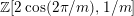 $\mathbb{Z}[2\cos (2\unicode[STIX]{x1D70B}/m),1/m]$
.
$\mathbb{Z}[2\cos (2\unicode[STIX]{x1D70B}/m),1/m]$
.
Lemma 27. Let
 $m\in \mathbb{N}_{{\geqslant}1}$
, and let
$m\in \mathbb{N}_{{\geqslant}1}$
, and let
 $k$
be a good ring for
$k$
be a good ring for
 $I_{2}(m)$
. The following assertions are true.
$I_{2}(m)$
. The following assertions are true.
-
(1)
$2\cos (a(2\unicode[STIX]{x1D70B}/m)),4\cos (a(\unicode[STIX]{x1D70B}/m))^{2}\in k$
for all
$a\in \mathbb{Z}$
. -
(2)
$4\cos (a(\unicode[STIX]{x1D70B}/m))^{2}\in k^{\times }$
for all
$a\in \mathbb{Z}\setminus (m/2)\mathbb{Z}$
. -
(3)
$4\cos (a(\unicode[STIX]{x1D70B}/m))^{2}-4\cos (b(\unicode[STIX]{x1D70B}/m))^{2}\in k^{\times }$
for all
$1\leqslant a<b\leqslant \left\lfloor m/2\right\rfloor$
.


Proof. Set
 $\unicode[STIX]{x1D701}_{n}:=\exp (2\unicode[STIX]{x1D70B}i/n)$
for all
$\unicode[STIX]{x1D701}_{n}:=\exp (2\unicode[STIX]{x1D70B}i/n)$
for all
 $n\in \mathbb{N}_{{\geqslant}1}$
. With this notation,
$n\in \mathbb{N}_{{\geqslant}1}$
. With this notation,
 $2\cos (a(2\unicode[STIX]{x1D70B}/n))=\unicode[STIX]{x1D701}_{n}^{a}+\unicode[STIX]{x1D701}_{n}^{-a}$
holds. It follows from
$2\cos (a(2\unicode[STIX]{x1D70B}/n))=\unicode[STIX]{x1D701}_{n}^{a}+\unicode[STIX]{x1D701}_{n}^{-a}$
holds. It follows from
 $T^{a}+T^{-a}\in \mathbb{Z}[T+T^{-1}]$
that
$T^{a}+T^{-a}\in \mathbb{Z}[T+T^{-1}]$
that
 $2\cos (a(2\unicode[STIX]{x1D70B}/n))\in k$
for all
$2\cos (a(2\unicode[STIX]{x1D70B}/n))\in k$
for all
 $a\in \mathbb{Z}$
. The fact that
$a\in \mathbb{Z}$
. The fact that
 $4\cos (a(\unicode[STIX]{x1D70B}/m))^{2}\in k$
follows from the double-angle formula
$4\cos (a(\unicode[STIX]{x1D70B}/m))^{2}\in k$
follows from the double-angle formula
 $2\cos (\unicode[STIX]{x1D703}/2)^{2}=\cos (\unicode[STIX]{x1D703})+1$
.
$2\cos (\unicode[STIX]{x1D703}/2)^{2}=\cos (\unicode[STIX]{x1D703})+1$
.
The proofs of the second and third claims use that
 $$\begin{eqnarray}\mathbb{Z}\biggl[2\cos \biggl(\frac{2\unicode[STIX]{x1D70B}}{n}\biggr)\biggr]=\mathbb{Z}[\unicode[STIX]{x1D701}_{n}+\unicode[STIX]{x1D701}_{n}^{-1}]\subseteq \mathbb{Z}[\unicode[STIX]{x1D701}_{n}]\subseteq \mathbb{Z}[\unicode[STIX]{x1D701}_{nl}]\end{eqnarray}$$
are integral ring extensions for all
 $l\in \mathbb{N}_{{\geqslant}1}$
, and integral extensions
$l\in \mathbb{N}_{{\geqslant}1}$
, and integral extensions
 $R\subseteq S$
have the property
$R\subseteq S$
have the property
 $R\cap S^{\times }=R^{\times }$
. Therefore, it suffices to show that the elements are units in
$R\cap S^{\times }=R^{\times }$
. Therefore, it suffices to show that the elements are units in
 $\mathbb{Z}[\unicode[STIX]{x1D701}_{ml},1/m]$
for some
$\mathbb{Z}[\unicode[STIX]{x1D701}_{ml},1/m]$
for some
 $l\in \mathbb{N}_{{\geqslant}1}$
.
$l\in \mathbb{N}_{{\geqslant}1}$
.
Step 1.
 $4\cos (a(\unicode[STIX]{x1D70B}/m))^{2}$
is invertible for all
$4\cos (a(\unicode[STIX]{x1D70B}/m))^{2}$
is invertible for all
 $a\in \mathbb{Z}\setminus (m/2)\mathbb{Z}$
.
$a\in \mathbb{Z}\setminus (m/2)\mathbb{Z}$
.
This follows from
 $$\begin{eqnarray}\mathop{\prod }_{1\leqslant a<m/2}\biggl(2\cos \biggl(a\frac{\unicode[STIX]{x1D70B}}{m}\biggr)\biggr)^{2}=\left\{\begin{array}{@{}ll@{}}1\quad & \text{if}~2\nmid m,\\ {\displaystyle \frac{m}{2}}\quad & \text{if}~2\mid m,\end{array}\right.\end{eqnarray}$$
which is easily shown using
 $2\cos (a(\unicode[STIX]{x1D70B}/m))=\unicode[STIX]{x1D701}_{2m}^{a}+\unicode[STIX]{x1D701}_{2m}^{-a}$
. Therefore,
$2\cos (a(\unicode[STIX]{x1D70B}/m))=\unicode[STIX]{x1D701}_{2m}^{a}+\unicode[STIX]{x1D701}_{2m}^{-a}$
. Therefore,
 $4\cos (a(\unicode[STIX]{x1D70B}/m))^{2}$
is invertible too.
$4\cos (a(\unicode[STIX]{x1D70B}/m))^{2}$
is invertible too.
Step 2.
 $2\sin (a(\unicode[STIX]{x1D70B}/m))$
is invertible for all
$2\sin (a(\unicode[STIX]{x1D70B}/m))$
is invertible for all
 $a\in \mathbb{Z}\setminus m\mathbb{Z}$
.
$a\in \mathbb{Z}\setminus m\mathbb{Z}$
.
This follows from
 $$\begin{eqnarray}\mathop{\prod }_{a=1}^{m-1}2\sin \biggl(a\frac{\unicode[STIX]{x1D70B}}{m}\biggr)=m,\end{eqnarray}$$
which similarly can be shown using
 $2\sin (a(\unicode[STIX]{x1D70B}/m))=(1/i)(\unicode[STIX]{x1D701}_{2m}^{a}-\unicode[STIX]{x1D701}_{2m}^{-a})$
. Hence, all
$2\sin (a(\unicode[STIX]{x1D70B}/m))=(1/i)(\unicode[STIX]{x1D701}_{2m}^{a}-\unicode[STIX]{x1D701}_{2m}^{-a})$
. Hence, all
 $2\sin (a(\unicode[STIX]{x1D70B}/m))$
are units for
$2\sin (a(\unicode[STIX]{x1D70B}/m))$
are units for
 $a\in \mathbb{Z}\setminus m\mathbb{Z}$
. This then proves the third claim because
$a\in \mathbb{Z}\setminus m\mathbb{Z}$
. This then proves the third claim because
 $4\cos (a(\unicode[STIX]{x1D70B}/m))^{2}-4\cos (b(\unicode[STIX]{x1D70B}/m))^{2}=2\sin ((a+b)(\unicode[STIX]{x1D70B}/m))\cdot 2\sin ((a-b)(\unicode[STIX]{x1D70B}/m))$
holds.◻
$4\cos (a(\unicode[STIX]{x1D70B}/m))^{2}-4\cos (b(\unicode[STIX]{x1D70B}/m))^{2}=2\sin ((a+b)(\unicode[STIX]{x1D70B}/m))\cdot 2\sin ((a-b)(\unicode[STIX]{x1D70B}/m))$
holds.◻
Theorem 28. Let
 $m$
be a natural number
$m$
be a natural number
 ${\geqslant}3$
. The decomposition conjecture is true for all Coxeter groups of type
${\geqslant}3$
. The decomposition conjecture is true for all Coxeter groups of type
 $I_{2}(m)$
.
$I_{2}(m)$
.
Proof. The idea of the proof is to use a spectral decomposition of the loops
 $X_{1,2}X_{2,1}$
and
$X_{1,2}X_{2,1}$
and
 $X_{2,1}X_{1,2}$
, and construct a refinement of the compatibility graph as in Figure 2.
$X_{2,1}X_{1,2}$
, and construct a refinement of the compatibility graph as in Figure 2.
Figure 2. Refined compatibility graphs for
 $I_{2}(m)$
: left-hand side for
$I_{2}(m)$
: left-hand side for
 $m$
odd; right-hand side for
$m$
odd; right-hand side for
 $m$
even.
$m$
even.
The next important observation is that there are only two transversal edges if the rank of
 $(W,S)$
is two, namely
$(W,S)$
is two, namely
 $X_{1,2}$
and
$X_{1,2}$
and
 $X_{2,1}$
. Therefore, the only relations in
$X_{2,1}$
. Therefore, the only relations in
 $\unicode[STIX]{x1D6FA}$
of type
$\unicode[STIX]{x1D6FA}$
of type
 $(\unicode[STIX]{x1D6FC})$
are
$(\unicode[STIX]{x1D6FC})$
are
 $$\begin{eqnarray}0=\mathop{\sum }_{j=0}^{m-1}a_{j}\underbrace{X_{1,2}X_{2,1}\ldots }_{j}\qquad \text{and}\qquad 0=\mathop{\sum }_{j=0}^{m-1}a_{j}\underbrace{X_{2,1}X_{1,2}\ldots }_{j},\end{eqnarray}$$
where the
 $a_{j}$
are the coefficients of
$a_{j}$
are the coefficients of
 $\unicode[STIX]{x1D70F}_{m-1}$
.
$\unicode[STIX]{x1D70F}_{m-1}$
.
Step 1. Preparations.
For all
 $n\in \mathbb{N}$
, define
$n\in \mathbb{N}$
, define
 $\widetilde{\unicode[STIX]{x1D70F}}_{n}\in \mathbb{Z}[X]$
by
$\widetilde{\unicode[STIX]{x1D70F}}_{n}\in \mathbb{Z}[X]$
by
 $$\begin{eqnarray}\widetilde{\unicode[STIX]{x1D70F}}_{n}:=\left\{\begin{array}{@{}ll@{}}\unicode[STIX]{x1D70F}_{n}(\sqrt{X})\quad & \text{if}~2\mid n,\\ \unicode[STIX]{x1D70F}_{n}(\sqrt{X})\sqrt{X}\quad & \text{if}~2\nmid n.\end{array}\right.\end{eqnarray}$$
Recall that
 $\unicode[STIX]{x1D70F}_{n}$
is an even polynomial if
$\unicode[STIX]{x1D70F}_{n}$
is an even polynomial if
 $n$
is even and an odd polynomial if
$n$
is even and an odd polynomial if
 $n$
is odd. Therefore,
$n$
is odd. Therefore,
 $\widetilde{\unicode[STIX]{x1D70F}}_{n}$
really is a polynomial in
$\widetilde{\unicode[STIX]{x1D70F}}_{n}$
really is a polynomial in
 $X$
. It has degree
$X$
. It has degree
 $\lceil n/2\rceil$
and is monic. Since the
$\lceil n/2\rceil$
and is monic. Since the
 $n$
zeros of
$n$
zeros of
 $\unicode[STIX]{x1D70F}_{n}$
are given by
$\unicode[STIX]{x1D70F}_{n}$
are given by
 $2\cos ((a/n+1)\unicode[STIX]{x1D70B})$
for
$2\cos ((a/n+1)\unicode[STIX]{x1D70B})$
for
 $a=1,\ldots ,n$
(cf. [Reference Abramowitz and Stegun1, 22.16]), the zeros of
$a=1,\ldots ,n$
(cf. [Reference Abramowitz and Stegun1, 22.16]), the zeros of
 $\widetilde{\unicode[STIX]{x1D70F}}_{n}$
are given by
$\widetilde{\unicode[STIX]{x1D70F}}_{n}$
are given by
 $4\cos ((a/n+1)\unicode[STIX]{x1D70B})^{2}$
for
$4\cos ((a/n+1)\unicode[STIX]{x1D70B})^{2}$
for
 $a=1,\ldots ,\lceil n/2\rceil$
. In particular, the zeros of
$a=1,\ldots ,\lceil n/2\rceil$
. In particular, the zeros of
 $\widetilde{\unicode[STIX]{x1D70F}}_{m-1}$
are equal to
$\widetilde{\unicode[STIX]{x1D70F}}_{m-1}$
are equal to
 $\unicode[STIX]{x1D70E}_{a}:=4\cos (a(\unicode[STIX]{x1D70B}/m))^{2}$
for
$\unicode[STIX]{x1D70E}_{a}:=4\cos (a(\unicode[STIX]{x1D70B}/m))^{2}$
for
 $a=1,\ldots ,\lfloor m/2\rfloor$
.
$a=1,\ldots ,\lfloor m/2\rfloor$
.
Step 2. Construction of the idempotents.
If
 $m$
is odd, then the
$m$
is odd, then the
 $(\unicode[STIX]{x1D6FC})$
-type relations are already of the form
$(\unicode[STIX]{x1D6FC})$
-type relations are already of the form
 $\widetilde{\unicode[STIX]{x1D70F}}_{m-1}(X_{1,2}X_{2,1})=0$
and
$\widetilde{\unicode[STIX]{x1D70F}}_{m-1}(X_{1,2}X_{2,1})=0$
and
 $\widetilde{\unicode[STIX]{x1D70F}}_{m-1}(X_{2,1}X_{1,2})=0$
, respectively. If
$\widetilde{\unicode[STIX]{x1D70F}}_{m-1}(X_{2,1}X_{1,2})=0$
, respectively. If
 $m$
is even, then one can multiply the relation with
$m$
is even, then one can multiply the relation with
 $X_{1,2}$
and
$X_{1,2}$
and
 $X_{2,1}$
, and obtain the same equations.
$X_{2,1}$
, and obtain the same equations.
By defining
 $$\begin{eqnarray}\displaystyle F_{1,a} & := & \displaystyle \mathop{\prod }_{\substack{ b=1,\ldots ,\left\lfloor m/2\right\rfloor \\ b\neq a}}\frac{X_{1,2}X_{2,1}-\unicode[STIX]{x1D70E}_{b}E_{1}}{\unicode[STIX]{x1D70E}_{a}-\unicode[STIX]{x1D70E}_{b}}\qquad \text{and}\nonumber\\ \displaystyle F_{2,a} & := & \displaystyle \mathop{\prod }_{\substack{ b=1,\ldots ,\left\lfloor m/2\right\rfloor \\ b\neq a}}\frac{X_{2,1}X_{1,2}-\unicode[STIX]{x1D70E}_{b}E_{2}}{\unicode[STIX]{x1D70E}_{a}-\unicode[STIX]{x1D70E}_{b}}\end{eqnarray}$$
for all
 $a=1,\ldots ,\lfloor m/2\rfloor$
, we get a set of pairwise orthogonal idempotents
$a=1,\ldots ,\lfloor m/2\rfloor$
, we get a set of pairwise orthogonal idempotents
 $F_{1,a},F_{2,a}\in k\unicode[STIX]{x1D6FA}$
with
$F_{1,a},F_{2,a}\in k\unicode[STIX]{x1D6FA}$
with
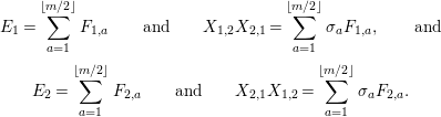 $$\begin{eqnarray}\displaystyle & \displaystyle E_{1}=\mathop{\sum }_{a=1}^{\lfloor m/2\rfloor }F_{1,a}\qquad \text{and}\qquad X_{1,2}X_{2,1}=\mathop{\sum }_{a=1}^{\lfloor m/2\rfloor }\unicode[STIX]{x1D70E}_{a}F_{1,a},\qquad \text{and} & \displaystyle \nonumber\\ \displaystyle & \displaystyle E_{2}=\mathop{\sum }_{a=1}^{\lfloor m/2\rfloor }F_{2,a}\qquad \text{and}\qquad X_{2,1}X_{1,2}=\mathop{\sum }_{a=1}^{\lfloor m/2\rfloor }\unicode[STIX]{x1D70E}_{a}F_{2,a}. & \displaystyle \nonumber\end{eqnarray}$$
Denote the irreducible characters of
 $W(I_{2}(m))$
of degree two by
$W(I_{2}(m))$
of degree two by
 $\unicode[STIX]{x1D706}_{a}$
for
$\unicode[STIX]{x1D706}_{a}$
for
 $a=1,\ldots ,m-1/2$
if
$a=1,\ldots ,m-1/2$
if
 $m$
is odd and
$m$
is odd and
 $a=1,\ldots ,m-2/2$
if
$a=1,\ldots ,m-2/2$
if
 $m$
is even. If
$m$
is even. If
 $m$
is even, there are two one-dimensional characters other than the trivial and the sign character, which will be denoted by
$m$
is even, there are two one-dimensional characters other than the trivial and the sign character, which will be denoted by
 $\unicode[STIX]{x1D716}_{1}$
and
$\unicode[STIX]{x1D716}_{1}$
and
 $\unicode[STIX]{x1D716}_{2}$
, respectively.
$\unicode[STIX]{x1D716}_{2}$
, respectively.
Now define the idempotents
 $(F^{\unicode[STIX]{x1D706}})_{\unicode[STIX]{x1D706}\in \text{Irr}(W)}$
as
$(F^{\unicode[STIX]{x1D706}})_{\unicode[STIX]{x1D706}\in \text{Irr}(W)}$
as
 $$\begin{eqnarray}\displaystyle F^{1} & = & \displaystyle E_{\emptyset },\nonumber\\ \displaystyle F^{\unicode[STIX]{x1D706}_{a}} & = & \displaystyle F_{1,a}+F_{2,a},\nonumber\\ \displaystyle F^{\text{sgn}} & = & \displaystyle E_{\{1,2\}},\nonumber\end{eqnarray}$$
and, if
 $m$
is even, define further
$m$
is even, define further
 $$\begin{eqnarray}\displaystyle F^{\unicode[STIX]{x1D716}_{1}} & = & \displaystyle F_{1,m/2}\qquad \text{and}\nonumber\\ \displaystyle F^{\unicode[STIX]{x1D716}_{2}} & = & \displaystyle F_{2,m/2}.\nonumber\end{eqnarray}$$
Now, (Z1) and (Z2) hold by construction. It remains to verify (Z3) and (Z4).
Step 3. Proving (Z3).
Now that we have the idempotents
 $F_{1,a},F_{2,a}$
splitting
$F_{1,a},F_{2,a}$
splitting
 $E_{1}$
and
$E_{1}$
and
 $E_{2}$
, respectively, we can consider
$E_{2}$
, respectively, we can consider
 $\unicode[STIX]{x1D6FA}$
as a quotient of the quiver which is obtained from
$\unicode[STIX]{x1D6FA}$
as a quotient of the quiver which is obtained from
 ${\mathcal{Q}}_{W}$
by splitting the vertices labeled
${\mathcal{Q}}_{W}$
by splitting the vertices labeled
 $\{1\}$
and
$\{1\}$
and
 $\{2\}$
into
$\{2\}$
into
 $\lfloor m/2\rfloor$
vertices each. A priori this could lead to the edge elements
$\lfloor m/2\rfloor$
vertices each. A priori this could lead to the edge elements
 $X_{1,2}$
,
$X_{1,2}$
,
 $X_{2,1}$
being split into
$X_{2,1}$
being split into
 $\lfloor m/2\rfloor ^{2}$
new edge elements
$\lfloor m/2\rfloor ^{2}$
new edge elements
 $F_{1,a}X_{1,2}F_{2,b}$
and
$F_{1,a}X_{1,2}F_{2,b}$
and
 $F_{2,a}X_{2,1}F_{1,b}$
, respectively. We show that this does not happen and instead all edge elements not depicted in Figure 2 vanish.
$F_{2,a}X_{2,1}F_{1,b}$
, respectively. We show that this does not happen and instead all edge elements not depicted in Figure 2 vanish.
This follows from Lemma 23 because
 $F_{1,a}$
can be obtained from
$F_{1,a}$
can be obtained from
 $F_{2,a}$
by idempotent transporting and vice versa. Note that
$F_{2,a}$
by idempotent transporting and vice versa. Note that
 $\unicode[STIX]{x1D70E}_{a}$
is invertible for
$\unicode[STIX]{x1D70E}_{a}$
is invertible for
 $1\leqslant a<m/2$
, and
$1\leqslant a<m/2$
, and
 $\unicode[STIX]{x1D70E}_{a}=0$
for
$\unicode[STIX]{x1D70E}_{a}=0$
for
 $a=m/2$
. This means that
$a=m/2$
. This means that
 $F_{1,m/2}$
and
$F_{1,m/2}$
and
 $F_{2,m/2}$
are the leftover idempotents. The lemma for idempotent transporting can be applied. Now, the following holds:
$F_{2,m/2}$
are the leftover idempotents. The lemma for idempotent transporting can be applied. Now, the following holds:
 $$\begin{eqnarray}\mathop{\sum }_{a=0}^{\lfloor m/2\rfloor }\unicode[STIX]{x1D70E}_{a}X_{1,2}F_{2,a}X_{2,1}=X_{1,2}\biggl(\underbrace{\mathop{\sum }_{a}\unicode[STIX]{x1D70E}_{a}F_{2,a}}_{=E_{2}}\biggr)X_{2,1}=X_{1,2}X_{2,1}=\mathop{\sum }_{a=0}^{\lfloor m/2\rfloor }\unicode[STIX]{x1D70E}_{a}F_{1,a}.\end{eqnarray}$$
Moreover, because
 $X_{1,2}F_{2,a}X_{2,1}$
is an idempotent, for
$X_{1,2}F_{2,a}X_{2,1}$
is an idempotent, for
 $1\leqslant a<m/2$
, both sides of the equation
$1\leqslant a<m/2$
, both sides of the equation
 $\sum _{a}\unicode[STIX]{x1D70E}_{a}X_{1,2}F_{2,a}X_{2,1}=\sum _{a}\unicode[STIX]{x1D70E}_{a}F_{1,a}$
describe the spectral decomposition of
$\sum _{a}\unicode[STIX]{x1D70E}_{a}X_{1,2}F_{2,a}X_{2,1}=\sum _{a}\unicode[STIX]{x1D70E}_{a}F_{1,a}$
describe the spectral decomposition of
 $X_{1,2}X_{2,1}$
. Since the
$X_{1,2}X_{2,1}$
. Since the
 $\unicode[STIX]{x1D70E}_{a}$
are pairwise distinct, one obtains
$\unicode[STIX]{x1D70E}_{a}$
are pairwise distinct, one obtains
 $F_{1,a}=X_{1,2}F_{2,a}X_{2,1}$
, and for symmetry reasons
$F_{1,a}=X_{1,2}F_{2,a}X_{2,1}$
, and for symmetry reasons
 $X_{2,1}F_{1,a}X_{1,2}=F_{2,a}$
for all
$X_{2,1}F_{1,a}X_{1,2}=F_{2,a}$
for all
 $1\leqslant a<m/2$
.
$1\leqslant a<m/2$
.
Now, Lemma 23 additionally implies
 $F_{1,a}X_{1,2}=X_{1,2}F_{2,a}$
, so that
$F_{1,a}X_{1,2}=X_{1,2}F_{2,a}$
, so that
 $F_{1,a}X_{1,2}F_{2,b}=0$
for
$F_{1,a}X_{1,2}F_{2,b}=0$
for
 $a\neq b$
. Moreover, for symmetry reasons, also
$a\neq b$
. Moreover, for symmetry reasons, also
 $F_{2,a}X_{2,1}F_{1,b}=0$
for
$F_{2,a}X_{2,1}F_{1,b}=0$
for
 $a\neq b$
.
$a\neq b$
.
If
 $m$
is even, then it is also true that there are no edges
$m$
is even, then it is also true that there are no edges
 $F_{1,m/2}\leftrightarrows F_{2,m/2}$
. This can be seen as follows. By construction,
$F_{1,m/2}\leftrightarrows F_{2,m/2}$
. This can be seen as follows. By construction,
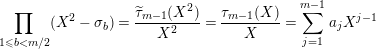 $$\begin{eqnarray}\mathop{\prod }_{1\leqslant b<m/2}(X^{2}-\unicode[STIX]{x1D70E}_{b})=\frac{\widetilde{\unicode[STIX]{x1D70F}}_{m-1}(X^{2})}{X^{2}}=\frac{\unicode[STIX]{x1D70F}_{m-1}(X)}{X}=\mathop{\sum }_{j=1}^{m-1}a_{j}X^{j-1}\end{eqnarray}$$
holds. By inserting
 $X_{2,1}X_{1,2}$
for
$X_{2,1}X_{1,2}$
for
 $X^{2}$
and multiplying by
$X^{2}$
and multiplying by
 $X_{1,2}$
, this gives
$X_{1,2}$
, this gives
 $$\begin{eqnarray}X_{1,2}\mathop{\prod }_{1\leqslant b<m/2}(X_{2,1}X_{1,2}-\unicode[STIX]{x1D70E}_{b})=\mathop{\sum }_{j=0}^{m-1}a_{j}\underbrace{X_{1,2}X_{2,1}\ldots }_{j\,\text{factors}}\overset{(\unicode[STIX]{x1D6FC})}{=}0.\end{eqnarray}$$
Now, multiplication with the denominator of (1) gives
 $X_{1,2}F_{2,m/2}=0$
, so that there are no edges from
$X_{1,2}F_{2,m/2}=0$
, so that there are no edges from
 $F_{2,m/2}$
to any vertex labeled with
$F_{2,m/2}$
to any vertex labeled with
 $\{1\}$
. Moreover, for symmetry reasons, there can be no edge from
$\{1\}$
. Moreover, for symmetry reasons, there can be no edge from
 $F_{1,m/2}$
to any vertex labeled with
$F_{1,m/2}$
to any vertex labeled with
 $\{2\}$
.
$\{2\}$
.
Therefore, the only edges that can exist are edges
 $F_{1,a}\leftrightarrows F_{2,a}$
, edges
$F_{1,a}\leftrightarrows F_{2,a}$
, edges
 $\emptyset \rightarrow F_{i,a}$
, the edge
$\emptyset \rightarrow F_{i,a}$
, the edge
 $\emptyset \rightarrow \{12\}$
and edges
$\emptyset \rightarrow \{12\}$
and edges
 $F_{i,a}\rightarrow \{12\}$
. This means that (Z3) is satisfied if we define a partial order on
$F_{i,a}\rightarrow \{12\}$
. This means that (Z3) is satisfied if we define a partial order on
 $\text{Irr}(W)$
by declaring
$\text{Irr}(W)$
by declaring
 $\text{sgn}$
as the top element, 1 as the bottom element and all other elements as mutually incomparable.
$\text{sgn}$
as the top element, 1 as the bottom element and all other elements as mutually incomparable.
Step 4. Proving (Z4).
For the characters of degree one, define
 $\unicode[STIX]{x1D713}_{\unicode[STIX]{x1D706}}:k^{1\times 1}\rightarrow F^{\unicode[STIX]{x1D706}}k\unicode[STIX]{x1D6FA}F^{\unicode[STIX]{x1D706}}$
by
$\unicode[STIX]{x1D713}_{\unicode[STIX]{x1D706}}:k^{1\times 1}\rightarrow F^{\unicode[STIX]{x1D706}}k\unicode[STIX]{x1D6FA}F^{\unicode[STIX]{x1D706}}$
by
 $\unicode[STIX]{x1D713}_{\unicode[STIX]{x1D706}}(e_{11}):=F^{\unicode[STIX]{x1D706}}$
. This homomorphism is surjective because of the lack of closed loops based at
$\unicode[STIX]{x1D713}_{\unicode[STIX]{x1D706}}(e_{11}):=F^{\unicode[STIX]{x1D706}}$
. This homomorphism is surjective because of the lack of closed loops based at
 $F^{\unicode[STIX]{x1D706}}$
in the quiver displayed in Figure 2. Therefore,
$F^{\unicode[STIX]{x1D706}}$
in the quiver displayed in Figure 2. Therefore,
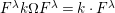 $F^{\unicode[STIX]{x1D706}}k\unicode[STIX]{x1D6FA}F^{\unicode[STIX]{x1D706}}=k\cdot F^{\unicode[STIX]{x1D706}}$
holds and
$F^{\unicode[STIX]{x1D706}}k\unicode[STIX]{x1D6FA}F^{\unicode[STIX]{x1D706}}=k\cdot F^{\unicode[STIX]{x1D706}}$
holds and
 $\unicode[STIX]{x1D713}_{\unicode[STIX]{x1D706}}$
is surjective.
$\unicode[STIX]{x1D713}_{\unicode[STIX]{x1D706}}$
is surjective.
For the characters of degree two, define
 $\unicode[STIX]{x1D713}_{\unicode[STIX]{x1D706}_{a}}:k^{2\times 2}\rightarrow F^{\unicode[STIX]{x1D706}_{a}}k\unicode[STIX]{x1D6FA}F^{\unicode[STIX]{x1D706}_{a}}$
by
$\unicode[STIX]{x1D713}_{\unicode[STIX]{x1D706}_{a}}:k^{2\times 2}\rightarrow F^{\unicode[STIX]{x1D706}_{a}}k\unicode[STIX]{x1D6FA}F^{\unicode[STIX]{x1D706}_{a}}$
by
 $$\begin{eqnarray}\left(\begin{array}{@{}cc@{}}e_{11} & e_{12}\\ e_{21} & e_{22}\end{array}\right)\mapsto \left(\begin{array}{@{}cc@{}}F_{1,a} & F^{\unicode[STIX]{x1D706}_{a}}X_{1,2}F^{\unicode[STIX]{x1D706}_{a}}\\ \unicode[STIX]{x1D70E}_{a}^{-1}F^{\unicode[STIX]{x1D706}_{a}}X_{2,1}F^{\unicode[STIX]{x1D706}_{a}} & F_{2,a}\end{array}\right).\end{eqnarray}$$
This is a well-defined algebra homomorphism by construction of
 $F^{\unicode[STIX]{x1D706}}$
. It is surjective because
$F^{\unicode[STIX]{x1D706}}$
. It is surjective because
 $F^{\unicode[STIX]{x1D706}_{a}}k\unicode[STIX]{x1D6FA}F^{\unicode[STIX]{x1D706}_{a}}$
is generated by the elements
$F^{\unicode[STIX]{x1D706}_{a}}k\unicode[STIX]{x1D6FA}F^{\unicode[STIX]{x1D706}_{a}}$
is generated by the elements
 $F_{I}^{\unicode[STIX]{x1D706}_{a}}$
and
$F_{I}^{\unicode[STIX]{x1D706}_{a}}$
and
 $F^{\unicode[STIX]{x1D706}_{a}}X_{\mathit{IJ}}F^{\unicode[STIX]{x1D706}_{a}}$
, all of which are contained in the image of
$F^{\unicode[STIX]{x1D706}_{a}}X_{\mathit{IJ}}F^{\unicode[STIX]{x1D706}_{a}}$
, all of which are contained in the image of
 $\unicode[STIX]{x1D713}_{\unicode[STIX]{x1D706}_{a}}$
.◻
$\unicode[STIX]{x1D713}_{\unicode[STIX]{x1D706}_{a}}$
.◻
5.4 Rank 3
Theorem 29. The decomposition conjecture is true for type
 $A_{3}$
.
$A_{3}$
.
We do not prove this in detail, since it is very similar to (although not formally a consequence of) the proof for
 $A_{4}$
, which is presented in the next section. Full details can also be found in [Reference Hahn5, Section 4.5].
$A_{4}$
, which is presented in the next section. Full details can also be found in [Reference Hahn5, Section 4.5].
Theorem 30. The decomposition conjecture is true for type
 $B_{3}$
.
$B_{3}$
.
Proof. We aim for a refinement of the compatibility graph as depicted in Figure 3 (where inclusion edges are again omitted for the sake of clarity). The relations of type
 $(\unicode[STIX]{x1D6FC})$
are crucial for this undertaking. We write
$(\unicode[STIX]{x1D6FC})$
are crucial for this undertaking. We write
 $(\unicode[STIX]{x1D6FC}^{st})$
to denote that we have used the relation of type
$(\unicode[STIX]{x1D6FC}^{st})$
to denote that we have used the relation of type
 $(\unicode[STIX]{x1D6FC})$
belonging to the edge
$(\unicode[STIX]{x1D6FC})$
belonging to the edge
 $s-t$
of the Dynkin diagram.
$s-t$
of the Dynkin diagram.
Figure 3. Refined compatibility graph of
 $B_{3}$
.
$B_{3}$
.
First, note that every good ring for
 $B_{3}$
contains
$B_{3}$
contains
 $\mathbb{Z}[1/2]$
, so that one is allowed to divide by two.
$\mathbb{Z}[1/2]$
, so that one is allowed to divide by two.
Step 1. (Z1) and (Z2).
We define elements
 $F_{I}^{\unicode[STIX]{x1D706},\unicode[STIX]{x1D707}}$
for all
$F_{I}^{\unicode[STIX]{x1D706},\unicode[STIX]{x1D707}}$
for all
 $I\subseteq S$
and all
$I\subseteq S$
and all
 $(\unicode[STIX]{x1D706},\unicode[STIX]{x1D707})\in \text{Irr}(W)$
according to Table 1, where absent entries are understood to be defined as zero. We therefore prove that the
$(\unicode[STIX]{x1D706},\unicode[STIX]{x1D707})\in \text{Irr}(W)$
according to Table 1, where absent entries are understood to be defined as zero. We therefore prove that the
 $F_{I}^{\unicode[STIX]{x1D706},\unicode[STIX]{x1D707}}$
are pairwise orthogonal idempotents with
$F_{I}^{\unicode[STIX]{x1D706},\unicode[STIX]{x1D707}}$
are pairwise orthogonal idempotents with
 $E_{I}=\sum _{\unicode[STIX]{x1D706},\unicode[STIX]{x1D707}}F_{I}^{\unicode[STIX]{x1D706},\unicode[STIX]{x1D707}}$
.
$E_{I}=\sum _{\unicode[STIX]{x1D706},\unicode[STIX]{x1D707}}F_{I}^{\unicode[STIX]{x1D706},\unicode[STIX]{x1D707}}$
.
Table 1. Expressions for the vertex idempotents of the refined compatibility graph of
 $B_{3}$
arranged in the same positions as the vertices in Figure 3.
$B_{3}$
arranged in the same positions as the vertices in Figure 3.

The
 $(\unicode[STIX]{x1D6FC}^{21})$
-relation
$(\unicode[STIX]{x1D6FC}^{21})$
-relation
 $E_{2}=X_{2,1}X_{1,2}$
implies that
$E_{2}=X_{2,1}X_{1,2}$
implies that
 $F_{1}^{\prime }:=X_{1,2}X_{2,1}$
is an idempotent
$F_{1}^{\prime }:=X_{1,2}X_{2,1}$
is an idempotent
 ${\leqslant}E_{1}$
. The
${\leqslant}E_{1}$
. The
 $(\unicode[STIX]{x1D6FC}^{12})$
-relation
$(\unicode[STIX]{x1D6FC}^{12})$
-relation
 $$\begin{eqnarray}E_{1}=X_{1,2}X_{2,1}+X_{1,02}X_{02,1}\end{eqnarray}$$
implies that
 $F_{1}^{\prime \prime }:=X_{1,02}X_{02,1}$
also is an idempotent
$F_{1}^{\prime \prime }:=X_{1,02}X_{02,1}$
also is an idempotent
 ${\leqslant}E_{1}$
which is orthogonal to
${\leqslant}E_{1}$
which is orthogonal to
 $F_{1}^{\prime }$
. These two idempotents are decomposed further.
$F_{1}^{\prime }$
. These two idempotents are decomposed further.
Recall that relations of type
 $(\unicode[STIX]{x1D6FC})$
use the polynomial
$(\unicode[STIX]{x1D6FC})$
use the polynomial
 $\unicode[STIX]{x1D70F}_{m-1}$
, which for
$\unicode[STIX]{x1D70F}_{m-1}$
, which for
 $m=4$
has the form
$m=4$
has the form
 $\unicode[STIX]{x1D70F}_{4-1}(T)=T^{3}-2T$
. Therefore,
$\unicode[STIX]{x1D70F}_{4-1}(T)=T^{3}-2T$
. Therefore,
 $(\unicode[STIX]{x1D6FC}^{01})$
and
$(\unicode[STIX]{x1D6FC}^{01})$
and
 $(\unicode[STIX]{x1D6FC}^{10})$
imply
$(\unicode[STIX]{x1D6FC}^{10})$
imply
 $$\begin{eqnarray}\displaystyle 0 & = & \displaystyle X_{0,1}X_{1,0}X_{0,1}+X_{0,1}X_{1,02}X_{02,1}-2X_{0,1},\end{eqnarray}$$
 $$\begin{eqnarray}\displaystyle 0 & = & \displaystyle X_{1,0}X_{0,1}X_{1,0}+X_{1,02}X_{02,1}X_{1,0}-2X_{1,0}.\end{eqnarray}$$
By setting
 $f:=X_{1,0}X_{0,1}$
, multiplying the first equation by
$f:=X_{1,0}X_{0,1}$
, multiplying the first equation by
 $X_{1,0}$
from the left and the second by
$X_{1,0}$
from the left and the second by
 $X_{0,1}$
from the right, we obtain
$X_{0,1}$
from the right, we obtain
 $$\begin{eqnarray}\displaystyle 0 & = & \displaystyle f^{2}+fF_{1}^{\prime \prime }-2f,\end{eqnarray}$$
 $$\begin{eqnarray}\displaystyle 0 & = & \displaystyle f^{2}+F_{1}^{\prime \prime }f-2f.\end{eqnarray}$$
Thus,
 $$\begin{eqnarray}f^{\prime \prime }:=fF_{1}^{\prime \prime }=F_{1}^{\prime \prime }f\qquad \text{and}\qquad f^{\prime }:=fF_{1}^{\prime }=F_{1}^{\prime }f\end{eqnarray}$$
are idempotents. We multiply (4) with
 $F_{1}^{\prime \prime }$
and (5) with
$F_{1}^{\prime \prime }$
and (5) with
 $F_{1}^{\prime }$
, and obtain
$F_{1}^{\prime }$
, and obtain
 $$\begin{eqnarray}\displaystyle 0 & = & \displaystyle f^{\prime \prime 2}-f^{\prime \prime },\end{eqnarray}$$
 $$\begin{eqnarray}\displaystyle 0 & = & \displaystyle f^{\prime 2}-2f^{\prime }.\end{eqnarray}$$
This gives us the following decomposition into orthogonal idempotents:
With these notations, 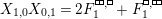 holds. We see that the other idempotents are now related either by transporting of idempotents along
 $\{1\}\rightarrow \{0\}$
or
$\{1\}\rightarrow \{0\}$
or
 $\{1\}\rightarrow \{2\}$
, or by applying the antiautomorphism
$\{1\}\rightarrow \{2\}$
, or by applying the antiautomorphism
 $\unicode[STIX]{x1D6FF}$
to previously constructed elements. In particular, the
$\unicode[STIX]{x1D6FF}$
to previously constructed elements. In particular, the
 $F_{I}^{\unicode[STIX]{x1D706},\unicode[STIX]{x1D707}}$
defined in Table 1 are pairwise orthogonal idempotents.
$F_{I}^{\unicode[STIX]{x1D706},\unicode[STIX]{x1D707}}$
defined in Table 1 are pairwise orthogonal idempotents.
Step 3. Verifying (Z3).
We check that in Figure 3 only upward edges appear, so that the partial ordering on
 $\text{Irr}(W)$
can be read off from the picture. We in fact show that the only edges not depicted in Figure 3 are inclusion edges.
$\text{Irr}(W)$
can be read off from the picture. We in fact show that the only edges not depicted in Figure 3 are inclusion edges.
The following holds:
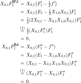
This means that there cannot be edges from ![]() or
or ![]() to vertices labeled with
to vertices labeled with
 $\{0\}$
. Since the idempotents labeled by
$\{0\}$
. Since the idempotents labeled by
 $\{0\}$
were defined by transport of idempotents, it follows from Lemma 23 that
$\{0\}$
were defined by transport of idempotents, it follows from Lemma 23 that  holds; that is, there are no edges from vertices labeled with
 $\{1\}$
to
$\{1\}$
to ![]()
Analogously, both  and
and  also hold. Therefore, there cannot be edges from vertices labeled with
 $\{0\}$
to
$\{0\}$
to ![]() or
or ![]() Again, it follows from Lemma 23 that
Again, it follows from Lemma 23 that  holds; that is, there are no edges from
 ![]() to vertices labeled with
to vertices labeled with
 $\{1\}$
.
$\{1\}$
.
Because the idempotents ![]() and
and ![]() were defined by transport of idempotents, there are no edges
were defined by transport of idempotents, there are no edges  or
or  Similarly, there are no edges
  or
or 
Now, we use the symmetry given by
 $\unicode[STIX]{x1D6FF}$
and obtain the same result for vertices labeled with
$\unicode[STIX]{x1D6FF}$
and obtain the same result for vertices labeled with
 $\{01\}$
,
$\{01\}$
,
 $\{02\}$
and
$\{02\}$
and
 $\{12\}$
.
$\{12\}$
.
It remains to verify that there are no edges  or
or  To this end, we prove that the idempotents
 ![]() and
and ![]() are also given by a transport of idempotents. This follows from an application of the
are also given by a transport of idempotents. This follows from an application of the
 $(\unicode[STIX]{x1D6FC}^{10})$
-relation:
$(\unicode[STIX]{x1D6FC}^{10})$
-relation:
 $$\begin{eqnarray}0=X_{02,1}X_{1,0}X_{0,1}+X_{02,1}X_{1,02}X_{02,1}+X_{02,12}X_{12,02}X_{02,1}-2X_{02,1}.\end{eqnarray}$$
Multiplying with
 $X_{1,02}$
from the left, and using
$X_{1,02}$
from the left, and using 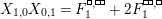 as well as
 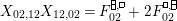 and
and
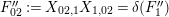 $F_{02}^{\prime \prime }:=X_{02,1}X_{1,02}=\unicode[STIX]{x1D6FF}(F_{1}^{\prime \prime })$
, we obtain
$F_{02}^{\prime \prime }:=X_{02,1}X_{1,02}=\unicode[STIX]{x1D6FF}(F_{1}^{\prime \prime })$
, we obtain
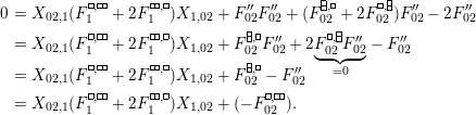
Hence, we obtain

The
 $(\unicode[STIX]{x1D6FC}^{21})$
-relation
$(\unicode[STIX]{x1D6FC}^{21})$
-relation
 $$\begin{eqnarray}0=X_{02,1}X_{1,2}\end{eqnarray}$$
implies
 $X_{02,1}F_{1}^{\prime }=0$
, so that
$X_{02,1}F_{1}^{\prime }=0$
, so that  because
  Therefore, we obtain
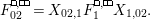
That is, ![]() is a transported idempotent along the edge
is a transported idempotent along the edge
 $\{02\}\leftrightarrows \{1\}$
. Because of
$\{02\}\leftrightarrows \{1\}$
. Because of 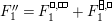 ,we also obtain
which, together with Lemma 23, implies that there are no edges other than the ones displayed in Figure 3 between vertices labeled with
 $\{1\}$
and
$\{1\}$
and
 $\{02\}$
. This shows that (Z3) holds.
$\{02\}$
. This shows that (Z3) holds.
Step 4. Verifying (Z4).
There is not much to do for the characters of degree one. We define
 $\unicode[STIX]{x1D713}_{\unicode[STIX]{x1D706},\unicode[STIX]{x1D707}}:\mathbb{Z}[1/2]^{1\times 1}\rightarrow F^{\unicode[STIX]{x1D706},\unicode[STIX]{x1D707}}\mathbb{Z}[1/2]\unicode[STIX]{x1D6FA}F^{\unicode[STIX]{x1D706},\unicode[STIX]{x1D707}}$
to be the only possible morphism, namely
$\unicode[STIX]{x1D713}_{\unicode[STIX]{x1D706},\unicode[STIX]{x1D707}}:\mathbb{Z}[1/2]^{1\times 1}\rightarrow F^{\unicode[STIX]{x1D706},\unicode[STIX]{x1D707}}\mathbb{Z}[1/2]\unicode[STIX]{x1D6FA}F^{\unicode[STIX]{x1D706},\unicode[STIX]{x1D707}}$
to be the only possible morphism, namely
 $\unicode[STIX]{x1D713}_{\unicode[STIX]{x1D706},\unicode[STIX]{x1D707}}(e_{11}):=F^{\unicode[STIX]{x1D706},\unicode[STIX]{x1D707}}$
. The surjectivity of these maps is automatic because the four components for the one-dimensional characters in the refined compatibility graph have no edges, and therefore
$\unicode[STIX]{x1D713}_{\unicode[STIX]{x1D706},\unicode[STIX]{x1D707}}(e_{11}):=F^{\unicode[STIX]{x1D706},\unicode[STIX]{x1D707}}$
. The surjectivity of these maps is automatic because the four components for the one-dimensional characters in the refined compatibility graph have no edges, and therefore
 $F^{\unicode[STIX]{x1D706},\unicode[STIX]{x1D707}}\mathbb{Z}[1/2]\unicode[STIX]{x1D6FA}F^{\unicode[STIX]{x1D706},\unicode[STIX]{x1D707}}=\mathbb{Z}[1/2]F^{\unicode[STIX]{x1D706},\unicode[STIX]{x1D707}}$
.
$F^{\unicode[STIX]{x1D706},\unicode[STIX]{x1D707}}\mathbb{Z}[1/2]\unicode[STIX]{x1D6FA}F^{\unicode[STIX]{x1D706},\unicode[STIX]{x1D707}}=\mathbb{Z}[1/2]F^{\unicode[STIX]{x1D706},\unicode[STIX]{x1D707}}$
.
Table 2. Morphisms
 $\unicode[STIX]{x1D713}_{\unicode[STIX]{x1D706},\unicode[STIX]{x1D707}}:\mathbb{Z}[1/2]^{d_{\unicode[STIX]{x1D706},\unicode[STIX]{x1D707}}\times d_{\unicode[STIX]{x1D706},\unicode[STIX]{x1D707}}}{\twoheadrightarrow}F^{\unicode[STIX]{x1D706},\unicode[STIX]{x1D707}}\mathbb{Z}[1/2]\unicode[STIX]{x1D6FA}F^{\unicode[STIX]{x1D706},\unicode[STIX]{x1D707}}$
for
$\unicode[STIX]{x1D713}_{\unicode[STIX]{x1D706},\unicode[STIX]{x1D707}}:\mathbb{Z}[1/2]^{d_{\unicode[STIX]{x1D706},\unicode[STIX]{x1D707}}\times d_{\unicode[STIX]{x1D706},\unicode[STIX]{x1D707}}}{\twoheadrightarrow}F^{\unicode[STIX]{x1D706},\unicode[STIX]{x1D707}}\mathbb{Z}[1/2]\unicode[STIX]{x1D6FA}F^{\unicode[STIX]{x1D706},\unicode[STIX]{x1D707}}$
for
 $2\leqslant d_{\unicode[STIX]{x1D706},\unicode[STIX]{x1D707}}\leqslant 3$
.
$2\leqslant d_{\unicode[STIX]{x1D706},\unicode[STIX]{x1D707}}\leqslant 3$
.

Table 2 lists all of the morphisms
 $\unicode[STIX]{x1D713}_{\unicode[STIX]{x1D706},\unicode[STIX]{x1D707}}:\mathbb{Z}[{\textstyle \frac{1}{2}}]^{d_{\unicode[STIX]{x1D706},\unicode[STIX]{x1D707}}\times d_{\unicode[STIX]{x1D706},\unicode[STIX]{x1D707}}}\rightarrow F^{\unicode[STIX]{x1D706},\unicode[STIX]{x1D707}}\mathbb{Z}[{\textstyle \frac{1}{2}}]\unicode[STIX]{x1D6FA}F^{\unicode[STIX]{x1D706},\unicode[STIX]{x1D707}}$
for the characters of degree two and three, where we use the notation
$\unicode[STIX]{x1D713}_{\unicode[STIX]{x1D706},\unicode[STIX]{x1D707}}:\mathbb{Z}[{\textstyle \frac{1}{2}}]^{d_{\unicode[STIX]{x1D706},\unicode[STIX]{x1D707}}\times d_{\unicode[STIX]{x1D706},\unicode[STIX]{x1D707}}}\rightarrow F^{\unicode[STIX]{x1D706},\unicode[STIX]{x1D707}}\mathbb{Z}[{\textstyle \frac{1}{2}}]\unicode[STIX]{x1D6FA}F^{\unicode[STIX]{x1D706},\unicode[STIX]{x1D707}}$
for the characters of degree two and three, where we use the notation
 $X_{\mathit{IJ}}^{\unicode[STIX]{x1D706},\unicode[STIX]{x1D707}}:=F^{\unicode[STIX]{x1D706},\unicode[STIX]{x1D707}}X_{\mathit{IJ}}F^{\unicode[STIX]{x1D706},\unicode[STIX]{x1D707}}$
.
$X_{\mathit{IJ}}^{\unicode[STIX]{x1D706},\unicode[STIX]{x1D707}}:=F^{\unicode[STIX]{x1D706},\unicode[STIX]{x1D707}}X_{\mathit{IJ}}F^{\unicode[STIX]{x1D706},\unicode[STIX]{x1D707}}$
.
We have used again that
 $\mathbb{Z}[1/2]^{d\times d}$
is the
$\mathbb{Z}[1/2]^{d\times d}$
is the
 $\mathbb{Z}[1/2]$
-algebra given by the presentation in Lemma 25. These relations are satisfied by construction of the
$\mathbb{Z}[1/2]$
-algebra given by the presentation in Lemma 25. These relations are satisfied by construction of the
 $F^{\unicode[STIX]{x1D706},\unicode[STIX]{x1D707}}$
, and therefore all of the maps in the table are well-defined algebra morphisms.
$F^{\unicode[STIX]{x1D706},\unicode[STIX]{x1D707}}$
, and therefore all of the maps in the table are well-defined algebra morphisms.
The construction of
 $\unicode[STIX]{x1D713}_{\unicode[STIX]{x1D706},\unicode[STIX]{x1D707}}$
ensures that all idempotents
$\unicode[STIX]{x1D713}_{\unicode[STIX]{x1D706},\unicode[STIX]{x1D707}}$
ensures that all idempotents
 $F_{I}^{\unicode[STIX]{x1D706},\unicode[STIX]{x1D707}}$
for all
$F_{I}^{\unicode[STIX]{x1D706},\unicode[STIX]{x1D707}}$
for all
 $I\subseteq S$
and all
$I\subseteq S$
and all
 $F^{\unicode[STIX]{x1D706},\unicode[STIX]{x1D707}}X_{\mathit{IJ}}F^{\unicode[STIX]{x1D706},\unicode[STIX]{x1D707}}$
for transversal edges
$F^{\unicode[STIX]{x1D706},\unicode[STIX]{x1D707}}X_{\mathit{IJ}}F^{\unicode[STIX]{x1D706},\unicode[STIX]{x1D707}}$
for transversal edges
 $I\leftrightarrows J$
are contained in the image of
$I\leftrightarrows J$
are contained in the image of
 $\unicode[STIX]{x1D713}_{\unicode[STIX]{x1D706},\unicode[STIX]{x1D707}}$
. For
$\unicode[STIX]{x1D713}_{\unicode[STIX]{x1D706},\unicode[STIX]{x1D707}}$
. For  , this is already enough to guarantee surjectivity, because all edges in the component of
 $F^{\unicode[STIX]{x1D706},\unicode[STIX]{x1D707}}$
are transversal edges.
$F^{\unicode[STIX]{x1D706},\unicode[STIX]{x1D707}}$
are transversal edges.
For ![]() , on the other hand, there could be an inclusion edge
, on the other hand, there could be an inclusion edge
 $\{0\}\rightarrow \{0,2\}$
, and for
$\{0\}\rightarrow \{0,2\}$
, and for ![]() ,there could be an inclusion edge
,there could be an inclusion edge
 $\{1\}\rightarrow \{1,2\}$
. To complete the proof, we show that this is not the case by using the
$\{1\}\rightarrow \{1,2\}$
. To complete the proof, we show that this is not the case by using the
 $(\unicode[STIX]{x1D6FD}^{20})$
-relation:
$(\unicode[STIX]{x1D6FD}^{20})$
-relation:
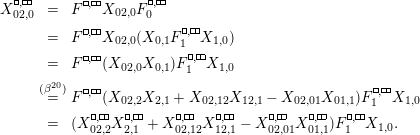
All summands within the brackets disappear because the ![]() component in the graph of Figure 3 has no vertices labeled
component in the graph of Figure 3 has no vertices labeled
 $\{2\}$
,
$\{2\}$
,
 $\{12\}$
or
$\{12\}$
or
 $\{01\}$
. Using the symmetry given by
$\{01\}$
. Using the symmetry given by
 $\unicode[STIX]{x1D6FF}$
, the equation
$\unicode[STIX]{x1D6FF}$
, the equation  also holds. ◻
5.5 Rank 4
Theorem 31. The decomposition conjecture is true for type
 $A_{4}$
.
$A_{4}$
.
Proof. We use an analogous strategy to that used before and use the relations of type
 $(\unicode[STIX]{x1D6FC})$
. Again, we write
$(\unicode[STIX]{x1D6FC})$
. Again, we write
 $(\unicode[STIX]{x1D6FC}^{st})$
to denote that we have used the relation of type
$(\unicode[STIX]{x1D6FC}^{st})$
to denote that we have used the relation of type
 $(\unicode[STIX]{x1D6FC})$
belonging to the edge
$(\unicode[STIX]{x1D6FC})$
belonging to the edge
 $s-t$
of the Dynkin diagram, and similarly for
$s-t$
of the Dynkin diagram, and similarly for
 $(\unicode[STIX]{x1D6FD})$
-type relations.
$(\unicode[STIX]{x1D6FD})$
-type relations.
Our goal is to decompose the compatibility graph as in Figure 4(a) (inclusion edges have been omitted for the sake of clarity).
Step 1. Verifying (Z1) and (Z2).
We define idempotents
 $F_{I}^{\unicode[STIX]{x1D706}}\leqslant E_{I}$
for all
$F_{I}^{\unicode[STIX]{x1D706}}\leqslant E_{I}$
for all
 $I\subseteq S,\unicode[STIX]{x1D706}\in \text{Irr}(W)$
, and set
$I\subseteq S,\unicode[STIX]{x1D706}\in \text{Irr}(W)$
, and set
 $F^{\unicode[STIX]{x1D706}}:=\sum _{I}F_{I}^{\unicode[STIX]{x1D706}}$
. First, note that, by Lemma 25, the idempotents of a matrix algebra are given by evaluating loops in the quiver. Looking at the quiver, we want to arrive at Figure 4(a). We therefore define the idempotents
$F^{\unicode[STIX]{x1D706}}:=\sum _{I}F_{I}^{\unicode[STIX]{x1D706}}$
. First, note that, by Lemma 25, the idempotents of a matrix algebra are given by evaluating loops in the quiver. Looking at the quiver, we want to arrive at Figure 4(a). We therefore define the idempotents
 $F_{I}^{\unicode[STIX]{x1D706}}$
either as one of the
$F_{I}^{\unicode[STIX]{x1D706}}$
either as one of the
 $E_{I}$
at the boundary of the compatibility graph or as loops connecting inner vertices to those outer vertices. More precisely, we use the definitions in Figure 4(b), where all
$E_{I}$
at the boundary of the compatibility graph or as loops connecting inner vertices to those outer vertices. More precisely, we use the definitions in Figure 4(b), where all
 $F_{I}^{\unicode[STIX]{x1D706}}$
not appearing there are understood to be defined as zero.
$F_{I}^{\unicode[STIX]{x1D706}}$
not appearing there are understood to be defined as zero.
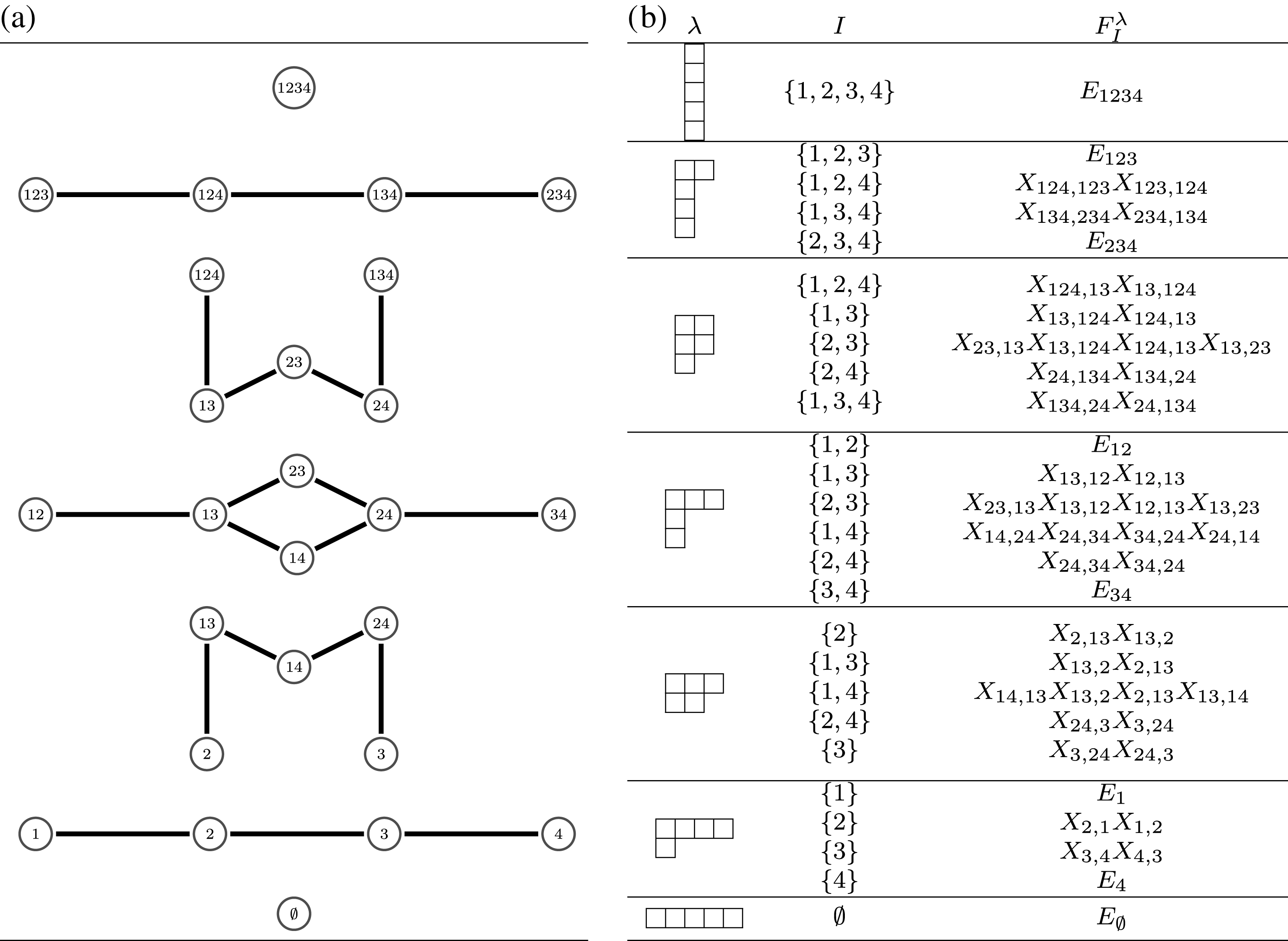
Figure 4. (a) The refined compatibility graph for
 $A_{4}$
and (b) vertex idempotents of the refined compatibility graph for
$A_{4}$
and (b) vertex idempotents of the refined compatibility graph for
 $A_{4}$
.
$A_{4}$
.
Once these elements have been defined, we have to prove that they are in fact idempotents and
 $E_{I}=\sum _{\unicode[STIX]{x1D706}}F_{I}^{\unicode[STIX]{x1D706}}$
is an orthogonal decomposition. (Z2) will then be satisfied because
$E_{I}=\sum _{\unicode[STIX]{x1D706}}F_{I}^{\unicode[STIX]{x1D706}}$
is an orthogonal decomposition. (Z2) will then be satisfied because
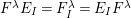 $F^{\unicode[STIX]{x1D706}}E_{I}=F_{I}^{\unicode[STIX]{x1D706}}=E_{I}F^{\unicode[STIX]{x1D706}}$
holds by definition.
$F^{\unicode[STIX]{x1D706}}E_{I}=F_{I}^{\unicode[STIX]{x1D706}}=E_{I}F^{\unicode[STIX]{x1D706}}$
holds by definition.
The
 $(\unicode[STIX]{x1D6FC}^{12})$
-relation implies
$(\unicode[STIX]{x1D6FC}^{12})$
-relation implies
 $$\begin{eqnarray}E_{1}=X_{1,2}X_{2,1},\end{eqnarray}$$
from which it follows that ![]() is an idempotent
is an idempotent
 ${\leqslant}E_{2}$
; namely, the idempotent obtained by transport of
${\leqslant}E_{2}$
; namely, the idempotent obtained by transport of
 $E_{1}\leqslant E_{1}$
along the edge
$E_{1}\leqslant E_{1}$
along the edge
 $\{1\}\rightarrow \{2\}$
. From the
$\{1\}\rightarrow \{2\}$
. From the
 $(\unicode[STIX]{x1D6FC}^{12})$
-relation
$(\unicode[STIX]{x1D6FC}^{12})$
-relation
 $$\begin{eqnarray}E_{2}=X_{2,1}X_{1,2}+X_{2,13}X_{13,2},\end{eqnarray}$$
we deduce that ![]() is the leftover idempotent of this transport. By applying the nontrivial graph automorphism, we obtain that
is the leftover idempotent of this transport. By applying the nontrivial graph automorphism, we obtain that ![]() and
and ![]() are idempotents as well, and by applying the antiautomorphism
are idempotents as well, and by applying the antiautomorphism
 $\unicode[STIX]{x1D6FF}$
, we find that
$\unicode[STIX]{x1D6FF}$
, we find that  and
and ![]() are idempotents too. Moreover, because Lemma 23 also gives us orthogonality with the leftover idempotent, we are done with all except the two-element subsets of
are idempotents too. Moreover, because Lemma 23 also gives us orthogonality with the leftover idempotent, we are done with all except the two-element subsets of
 $S$
.
$S$
.
By transporting 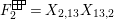 along
along
 $\{2\}\rightarrow \{13\}$
, we obtain the idempotent
$\{2\}\rightarrow \{13\}$
, we obtain the idempotent
By applying
 $\unicode[STIX]{x1D6FF}$
and the graph automorphism, we find that
$\unicode[STIX]{x1D6FF}$
and the graph automorphism, we find that  and
and ![]() are also idempotents.
are also idempotents.
The
 $(\unicode[STIX]{x1D6FC}^{23})$
-relation
$(\unicode[STIX]{x1D6FC}^{23})$
-relation
 $$\begin{eqnarray}E_{12}=X_{12,13}X_{13,12}\end{eqnarray}$$
implies that ![]() is the idempotent obtained by transporting
is the idempotent obtained by transporting
 $E_{12}$
along
$E_{12}$
along
 $\{12\}\rightarrow \{13\}$
.
$\{12\}\rightarrow \{13\}$
.
Considering the
 $(\unicode[STIX]{x1D6FC}^{32})$
-relations
$(\unicode[STIX]{x1D6FC}^{32})$
-relations
we find that  constitute an orthogonal decomposition of
 $E_{13}$
.
$E_{13}$
.
By applying the graph automorphism, we find that  and
and ![]() are pairwise idempotents as well.
are pairwise idempotents as well.
We are now almost done. We still need to look at the innermost vertices
 $\{2,3\}$
and
$\{2,3\}$
and
 $\{1,4\}$
of the compatibility graph. The following
$\{1,4\}$
of the compatibility graph. The following
 $(\unicode[STIX]{x1D6FC}^{34})$
-relation holds:
$(\unicode[STIX]{x1D6FC}^{34})$
-relation holds:
 $$\begin{eqnarray}E_{13}=X_{13,14}X_{14,13}+X_{13,124}X_{124,13}.\end{eqnarray}$$
This means that  Transporting these two idempotents along
 $\{13\}\rightarrow \{14\}$
, we obtain
$\{13\}\rightarrow \{14\}$
, we obtain ![]() and
and ![]() By symmetry,
By symmetry, ![]() and
and ![]() are idempotents as well.
are idempotents as well.
From the
 $(\unicode[STIX]{x1D6FC}^{43})$
- and
$(\unicode[STIX]{x1D6FC}^{43})$
- and
 $(\unicode[STIX]{x1D6FC}^{21})$
-relations
$(\unicode[STIX]{x1D6FC}^{21})$
-relations
 $$\begin{eqnarray}E_{14}=X_{14,13}X_{13,14}\qquad \text{and}\qquad E_{23}=X_{23,13}X_{13,23},\end{eqnarray}$$
we can infer that the two leftover idempotents for these transports vanish. Therefore, we get orthogonal decompositions  and
and  .
.
Step 2. Verifying (Z3).
We prove that the only edges between the components not displayed in Figure 4(a) are inclusion edges, from which it follows that the dominance ordering on
 $\{\unicode[STIX]{x1D706}\vdash 5\}$
is the sought-after partial ordering. Because we have constructed all idempotents by transport of idempotents, most transversal edges split into parallel edges. This eliminates almost all possible transversal edges between different components.
$\{\unicode[STIX]{x1D706}\vdash 5\}$
is the sought-after partial ordering. Because we have constructed all idempotents by transport of idempotents, most transversal edges split into parallel edges. This eliminates almost all possible transversal edges between different components.
The
 $(\unicode[STIX]{x1D6FC}^{32})$
-relation
$(\unicode[STIX]{x1D6FC}^{32})$
-relation
 $$\begin{eqnarray}X_{13,2}X_{2,3}=0\end{eqnarray}$$
implies that  , so that there is no transversal edge emanating from
  and going to
 ![]() . By symmetry, there are no transversal edges going from
. By symmetry, there are no transversal edges going from
 $E_{2}$
to
$E_{2}$
to ![]() , which shows that there are only inclusion edges between the
, which shows that there are only inclusion edges between the ![]() and the
and the ![]() component. Applying
component. Applying
 $\unicode[STIX]{x1D6FF}$
, we find the same between the
$\unicode[STIX]{x1D6FF}$
, we find the same between the ![]() and the
and the ![]() component.
component.
The only other possibility is transversal edges of the form
 $\{14\}\leftrightarrows \{24\}$
and
$\{14\}\leftrightarrows \{24\}$
and
 $\{23\}\leftrightarrows \{24\}$
, because we have not used idempotent transport along these edges. Instead, we worked with
$\{23\}\leftrightarrows \{24\}$
, because we have not used idempotent transport along these edges. Instead, we worked with
 $\{13\}\leftrightarrows \{14\}$
and
$\{13\}\leftrightarrows \{14\}$
and
 $\{13\}\leftrightarrows \{23\}$
.
$\{13\}\leftrightarrows \{23\}$
.
Consider the
 $(\unicode[STIX]{x1D6FD}^{24})$
-relation
$(\unicode[STIX]{x1D6FD}^{24})$
-relation
 $$\begin{eqnarray}X_{24,23}X_{23,13}+X_{24,2}X_{2,13}=X_{24,14}X_{14,13}+X_{24,134}X_{134,13},\end{eqnarray}$$
which implies
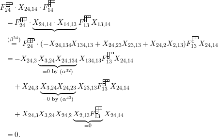
Similarly, combining the
 $(\unicode[STIX]{x1D6FD})$
- and
$(\unicode[STIX]{x1D6FD})$
- and
 $(\unicode[STIX]{x1D6FC})$
-relations, one shows that the transversal edge
$(\unicode[STIX]{x1D6FC})$
-relations, one shows that the transversal edge
 $\{14\}\rightarrow \{24\}$
splits into a pair of parallel edges, as displayed in Figure 4(a), and all four of the possible cross-component edges are indeed zero. Applying
$\{14\}\rightarrow \{24\}$
splits into a pair of parallel edges, as displayed in Figure 4(a), and all four of the possible cross-component edges are indeed zero. Applying
 $\unicode[STIX]{x1D6FF}$
, we find that the same holds between the
$\unicode[STIX]{x1D6FF}$
, we find that the same holds between the ![]() and the
and the ![]() component.
component.
This shows that, even for the edges
 $\{14\}\leftrightarrows \{24\}$
and
$\{14\}\leftrightarrows \{24\}$
and
 $\{23\}\leftrightarrows \{24\}$
, the idempotents on both sides are given by transporting idempotents, and hence there can only be parallel edges, as depicted in Figure 4(a). The only other possible edges are those not depicted in this picture; in other words, the inclusion edges.
$\{23\}\leftrightarrows \{24\}$
, the idempotents on both sides are given by transporting idempotents, and hence there can only be parallel edges, as depicted in Figure 4(a). The only other possible edges are those not depicted in this picture; in other words, the inclusion edges.
Step 3. Verifying (Z4).
We construct surjective homomorphisms
 $\unicode[STIX]{x1D713}_{\unicode[STIX]{x1D706}}:\mathbb{Z}^{d_{\unicode[STIX]{x1D706}}\times d_{\unicode[STIX]{x1D706}}}\rightarrow F^{\unicode[STIX]{x1D706}}\unicode[STIX]{x1D6FA}F^{\unicode[STIX]{x1D706}}$
. We use the presentation of
$\unicode[STIX]{x1D713}_{\unicode[STIX]{x1D706}}:\mathbb{Z}^{d_{\unicode[STIX]{x1D706}}\times d_{\unicode[STIX]{x1D706}}}\rightarrow F^{\unicode[STIX]{x1D706}}\unicode[STIX]{x1D6FA}F^{\unicode[STIX]{x1D706}}$
. We use the presentation of
 $\mathbb{Z}^{d_{\unicode[STIX]{x1D706}}\times d_{\unicode[STIX]{x1D706}}}$
from Lemma 25.
$\mathbb{Z}^{d_{\unicode[STIX]{x1D706}}\times d_{\unicode[STIX]{x1D706}}}$
from Lemma 25.
We use the abbreviation
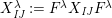 $X_{\mathit{IJ}}^{\unicode[STIX]{x1D706}}:=F^{\unicode[STIX]{x1D706}}X_{\mathit{IJ}}F^{\unicode[STIX]{x1D706}}$
. By construction, the equation
$X_{\mathit{IJ}}^{\unicode[STIX]{x1D706}}:=F^{\unicode[STIX]{x1D706}}X_{\mathit{IJ}}F^{\unicode[STIX]{x1D706}}$
. By construction, the equation
 $X_{\mathit{IJ}}^{\unicode[STIX]{x1D706}}X_{\mathit{JI}}^{\unicode[STIX]{x1D706}}=F_{I}^{\unicode[STIX]{x1D706}}$
holds for all transversal edges
$X_{\mathit{IJ}}^{\unicode[STIX]{x1D706}}X_{\mathit{JI}}^{\unicode[STIX]{x1D706}}=F_{I}^{\unicode[STIX]{x1D706}}$
holds for all transversal edges
 $I\leftrightarrows J$
if
$I\leftrightarrows J$
if
 $F_{I}^{\unicode[STIX]{x1D706}}$
and
$F_{I}^{\unicode[STIX]{x1D706}}$
and
 $F_{J}^{\unicode[STIX]{x1D706}}$
are both nonzero, as well as
$F_{J}^{\unicode[STIX]{x1D706}}$
are both nonzero, as well as
 $X_{\mathit{IJ}}^{\unicode[STIX]{x1D706}}=X_{\mathit{JI}}^{\unicode[STIX]{x1D706}}=0$
otherwise.
$X_{\mathit{IJ}}^{\unicode[STIX]{x1D706}}=X_{\mathit{JI}}^{\unicode[STIX]{x1D706}}=0$
otherwise.
If we denote the vertices of a component in Figure 4(a) with its index set (which is possible without conflicts since no index set occurs more than once), then
 $$\begin{eqnarray}\unicode[STIX]{x1D713}_{\unicode[STIX]{x1D706}}:\mathbb{Z}^{d_{\unicode[STIX]{x1D706}}\times d_{\unicode[STIX]{x1D706}}}\rightarrow F^{\unicode[STIX]{x1D706}}\unicode[STIX]{x1D6FA}F^{\unicode[STIX]{x1D706}},e_{II}\mapsto F_{I}^{\unicode[STIX]{x1D706}},e_{\mathit{IJ}}\mapsto X_{\mathit{IJ}}^{\unicode[STIX]{x1D706}}\end{eqnarray}$$
defines a morphism
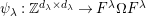 $\unicode[STIX]{x1D713}_{\unicode[STIX]{x1D706}}:\mathbb{Z}^{d_{\unicode[STIX]{x1D706}}\times d_{\unicode[STIX]{x1D706}}}\rightarrow F^{\unicode[STIX]{x1D706}}\unicode[STIX]{x1D6FA}F^{\unicode[STIX]{x1D706}}$
for those components that are straight lines without their inclusion edges; that is, all components except the one labeled with
$\unicode[STIX]{x1D713}_{\unicode[STIX]{x1D706}}:\mathbb{Z}^{d_{\unicode[STIX]{x1D706}}\times d_{\unicode[STIX]{x1D706}}}\rightarrow F^{\unicode[STIX]{x1D706}}\unicode[STIX]{x1D6FA}F^{\unicode[STIX]{x1D706}}$
for those components that are straight lines without their inclusion edges; that is, all components except the one labeled with ![]() .We prove surjectivity of
.We prove surjectivity of
 $\unicode[STIX]{x1D713}_{\unicode[STIX]{x1D706}}$
, which is equivalent to showing that all
$\unicode[STIX]{x1D713}_{\unicode[STIX]{x1D706}}$
, which is equivalent to showing that all
 $X_{\mathit{IJ}}^{\unicode[STIX]{x1D706}}$
are contained in the image
$X_{\mathit{IJ}}^{\unicode[STIX]{x1D706}}$
are contained in the image
 $\unicode[STIX]{x1D713}_{\unicode[STIX]{x1D706}}$
. For the transversal edges, this is clear from the construction. Therefore, we are done for
$\unicode[STIX]{x1D713}_{\unicode[STIX]{x1D706}}$
. For the transversal edges, this is clear from the construction. Therefore, we are done for  ,
,![]() ,
, ![]() and
and ![]() .For
.For ![]() , we must consider the inclusion edges
, we must consider the inclusion edges
 $X_{13,3}$
and
$X_{13,3}$
and
 $X_{24,2}$
. We use the relations of type
$X_{24,2}$
. We use the relations of type
 $(\unicode[STIX]{x1D6FD})$
:
$(\unicode[STIX]{x1D6FD})$
:
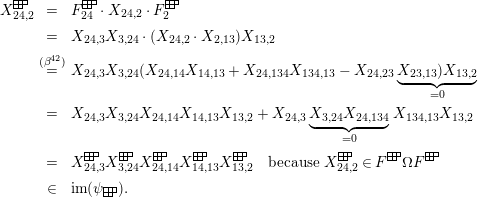
By applying the graph automorphism, we obtain 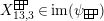 ,and by applying the antiautomorphism
 $\unicode[STIX]{x1D6FF}$
, we obtain
$\unicode[STIX]{x1D6FF}$
, we obtain 
 Therefore, all
 $X_{\mathit{IJ}}^{\unicode[STIX]{x1D706}}$
are contained in the image of
$X_{\mathit{IJ}}^{\unicode[STIX]{x1D706}}$
are contained in the image of
 $\unicode[STIX]{x1D713}_{\unicode[STIX]{x1D706}}$
for
$\unicode[STIX]{x1D713}_{\unicode[STIX]{x1D706}}$
for ![]() ,
, ![]() , and surjectivity holds in both cases.
, and surjectivity holds in both cases.
It remains to handle the case ![]() . We sort the two-element sets in the order
. We sort the two-element sets in the order
 $\{1,2\}$
,
$\{1,2\}$
,
 $\{1,3\}$
,
$\{1,3\}$
,
 $\{1,4\}$
,
$\{1,4\}$
,
 $\{2,3\}$
,
$\{2,3\}$
,
 $\{2,4\}$
,
$\{2,4\}$
,
 $\{3,4\}$
, and claim that the following homomorphism
$\{3,4\}$
, and claim that the following homomorphism  is well defined:
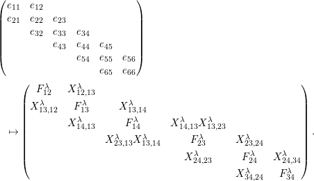 $$\begin{eqnarray}\displaystyle & & \displaystyle \left(\begin{array}{@{}cccccc@{}}e_{11} & e_{12} & & & & \\ e_{21} & e_{22} & e_{23} & & & \\ & e_{32} & e_{33} & e_{34} & & \\ & & e_{43} & e_{44} & e_{45} & \\ & & & e_{54} & e_{55} & e_{56}\\ & & & & e_{65} & e_{66}\end{array}\right)\nonumber\\ \displaystyle & & \displaystyle \quad \mapsto \left(\begin{array}{@{}cccccc@{}}F_{12}^{\unicode[STIX]{x1D706}} & X_{12,13}^{\unicode[STIX]{x1D706}} & & & & \\ X_{13,12}^{\unicode[STIX]{x1D706}} & F_{13}^{\unicode[STIX]{x1D706}} & X_{13,14}^{\unicode[STIX]{x1D706}} & & & \\ & X_{14,13}^{\unicode[STIX]{x1D706}} & F_{14}^{\unicode[STIX]{x1D706}} & X_{14,13}^{\unicode[STIX]{x1D706}}X_{13,23}^{\unicode[STIX]{x1D706}} & & \\ & & X_{23,13}^{\unicode[STIX]{x1D706}}X_{13,14}^{\unicode[STIX]{x1D706}} & F_{23}^{\unicode[STIX]{x1D706}} & X_{23,24}^{\unicode[STIX]{x1D706}} & \\ & & & X_{24,23}^{\unicode[STIX]{x1D706}} & F_{24}^{\unicode[STIX]{x1D706}} & X_{24,34}^{\unicode[STIX]{x1D706}}\\ & & & & X_{34,24}^{\unicode[STIX]{x1D706}} & F_{34}^{\unicode[STIX]{x1D706}}\end{array}\right).\nonumber\end{eqnarray}$$
Most relations from Lemma 25 are satisfied by construction of the idempotents. We still need to verify
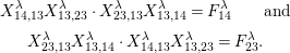 $$\begin{eqnarray}\displaystyle & \displaystyle X_{14,13}^{\unicode[STIX]{x1D706}}X_{13,23}^{\unicode[STIX]{x1D706}}\cdot X_{23,13}^{\unicode[STIX]{x1D706}}X_{13,14}^{\unicode[STIX]{x1D706}}=F_{14}^{\unicode[STIX]{x1D706}}\qquad \text{and} & \displaystyle \nonumber\\ \displaystyle & \displaystyle X_{23,13}^{\unicode[STIX]{x1D706}}X_{13,14}^{\unicode[STIX]{x1D706}}\cdot X_{14,13}^{\unicode[STIX]{x1D706}}X_{13,23}^{\unicode[STIX]{x1D706}}=F_{23}^{\unicode[STIX]{x1D706}}. & \displaystyle \nonumber\end{eqnarray}$$
These equations follow from the
 $(\unicode[STIX]{x1D6FC})$
-relations
$(\unicode[STIX]{x1D6FC})$
-relations
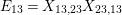 $E_{13}=X_{13,23}X_{23,13}$
and
$E_{13}=X_{13,23}X_{23,13}$
and
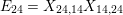 $E_{24}=X_{24,14}X_{14,24}$
.
$E_{24}=X_{24,14}X_{14,24}$
.
We verify the surjectivity of
 $\unicode[STIX]{x1D713}_{\unicode[STIX]{x1D706}}$
. By construction, most
$\unicode[STIX]{x1D713}_{\unicode[STIX]{x1D706}}$
. By construction, most
 $X_{\mathit{IJ}}^{\unicode[STIX]{x1D706}}$
are already contained in the image. We only have to consider the edges between
$X_{\mathit{IJ}}^{\unicode[STIX]{x1D706}}$
are already contained in the image. We only have to consider the edges between
 $F_{14}^{\unicode[STIX]{x1D706}}\leftrightarrows F_{24}^{\unicode[STIX]{x1D706}}$
and
$F_{14}^{\unicode[STIX]{x1D706}}\leftrightarrows F_{24}^{\unicode[STIX]{x1D706}}$
and
 $F_{13}^{\unicode[STIX]{x1D706}}\leftrightarrows F_{23}^{\unicode[STIX]{x1D706}}$
:
$F_{13}^{\unicode[STIX]{x1D706}}\leftrightarrows F_{23}^{\unicode[STIX]{x1D706}}$
:
 $$\begin{eqnarray}\displaystyle X_{23,13}^{\unicode[STIX]{x1D706}} & = & \displaystyle X_{23,13}^{\unicode[STIX]{x1D706}}F_{13}^{\unicode[STIX]{x1D706}}\nonumber\\ \displaystyle & = & \displaystyle X_{23,13}^{\unicode[STIX]{x1D706}}(X_{13,14}^{\unicode[STIX]{x1D706}}X_{14,13}^{\unicode[STIX]{x1D706}})\nonumber\\ \displaystyle & = & \displaystyle (X_{23,13}^{\unicode[STIX]{x1D706}}X_{13,14}^{\unicode[STIX]{x1D706}})X_{14,13}^{\unicode[STIX]{x1D706}}\in \text{im}(\unicode[STIX]{x1D713}_{\unicode[STIX]{x1D706}})\nonumber\end{eqnarray}$$
and
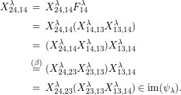 $$\begin{eqnarray}\displaystyle X_{24,14}^{\unicode[STIX]{x1D706}} & = & \displaystyle X_{24,14}^{\unicode[STIX]{x1D706}}F_{14}^{\unicode[STIX]{x1D706}}\nonumber\\ \displaystyle & = & \displaystyle X_{24,14}^{\unicode[STIX]{x1D706}}(X_{14,13}^{\unicode[STIX]{x1D706}}X_{13,14}^{\unicode[STIX]{x1D706}})\nonumber\\ \displaystyle & = & \displaystyle (X_{24,14}^{\unicode[STIX]{x1D706}}X_{14,13}^{\unicode[STIX]{x1D706}})X_{13,14}^{\unicode[STIX]{x1D706}}\nonumber\\ \displaystyle & \overset{(\unicode[STIX]{x1D6FD})}{=} & \displaystyle (X_{24,23}^{\unicode[STIX]{x1D706}}X_{23,13}^{\unicode[STIX]{x1D706}})X_{13,14}^{\unicode[STIX]{x1D706}}\nonumber\\ \displaystyle & = & \displaystyle X_{24,23}^{\unicode[STIX]{x1D706}}(X_{23,13}^{\unicode[STIX]{x1D706}}X_{13,14}^{\unicode[STIX]{x1D706}})\in \text{im}(\unicode[STIX]{x1D713}_{\unicode[STIX]{x1D706}}).\nonumber\end{eqnarray}$$
Applying
 $\unicode[STIX]{x1D6FF}$
, we find
$\unicode[STIX]{x1D6FF}$
, we find
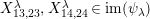 $X_{13,23}^{\unicode[STIX]{x1D706}},X_{14,24}^{\unicode[STIX]{x1D706}}\in \text{im}(\unicode[STIX]{x1D713}_{\unicode[STIX]{x1D706}})$
as well. Therefore,
$X_{13,23}^{\unicode[STIX]{x1D706}},X_{14,24}^{\unicode[STIX]{x1D706}}\in \text{im}(\unicode[STIX]{x1D713}_{\unicode[STIX]{x1D706}})$
as well. Therefore,
 $\unicode[STIX]{x1D713}_{\unicode[STIX]{x1D706}}$
is surjective.◻
$\unicode[STIX]{x1D713}_{\unicode[STIX]{x1D706}}$
is surjective.◻


