


Non-technical Summary
A primary tenet of the evolutionary theory of punctuated equilibria is that species are characterized by stasis (little to no net morphological change during their histories), rather than gradual directional change. Although stasis has been recognized in the fossil record of many species during the past ~50 years since punctuated equilibria was proposed, the causes of stasis remain unclear.
We argue here that a promising explanation for stasis is coevolutionary alternation. This hypothesis addresses how antagonists (e.g., predators or parasites and their groups of victims) evolve in response to one another. According to coevolutionary alternation, populations will differ in patterns of predator preferences and prey defenses. Prey that are preferred by the predator will evolve increased defenses, leading the predator to evolve preferences for less-defended prey. The new preferred prey will then evolve increased defenses, while the formerly preferred prey lose defenses, with consequent change in predator preferences. Because different populations will be at different stages in this process, the geographic structure of populations can produce stasis in those traits across the species as a whole. We suggest such coevolutionary alternation of predator and prey could be modeled statistically using coupled stochastic differential equations (SDEs), which have been used to study correlative and causal connections among time series. We make recommendations for how SDEs might be used to model the coevolutionary feedback of predator and prey populations evolving in response to one another across space and changing environments.
Introduction
A key component of Eldredge and Gould’s (Reference Eldredge, Gould and Schopf1972) concept of punctuated equilibria (PE) is the stability of species (stasis) throughout most of their evolutionary histories. Stasis was not defined as absolute invariance, but as little or no net morphological change within the history of a species, with temporal fluctuations not exceeding the range of variation occurring spatially at any one time (Gould Reference Gould2002; Lieberman Reference Lieberman, Allmon, Kelley and Ross2009). Gould (Reference Gould2002: p. 874) considered the concept of stasis to be PE’s biggest contribution to evolutionary science.
Eldredge and Gould’s seminal paper spurred numerous studies of tempo and mode in individual lineages, with qualitative reviews of this literature generally concluding that stasis is the most common pattern within species (e.g., Jackson and Cheetham Reference Jackson and Cheetham1999; Eldredge et al. Reference Eldredge, Thompson, Brakefield, Gavrilets, Jablonski, Jackson, Lenski, Lieberman, McPeek and Miller2005; Geary Reference Geary, Allmon, Kelley and Ross2009; Lieberman Reference Lieberman, Allmon, Kelley and Ross2009; but see Voje et al. [Reference Voje, Martino and Porto2020] for refutation of a classic study). The predominance of stasis was supported by Hunt (Reference Hunt2007), who developed a model-ranking approach to measure statistical support for three models of evolution: directional change, unbiased random walk, and stasis. When this model-ranking approach was applied to >250 sequences of morphological traits, only 5% of sequences showed directional evolution as the most strongly supported. Subsequent analyses applying similar techniques to expanded data compilations have also found directional change to be rare (Hopkins and Lidgard Reference Hopkins and Lidgard2012; Hunt et al. Reference Hunt, Hopkins and Lidgard2015). Although these analyses found variation in evolutionary mode among individual traits of many lineages, stasis was still common (in 63% of lineages at some point in their histories), even when testing more complex models that included punctuated change and shifts in mode of evolution (Hunt et al. Reference Hunt, Hopkins and Lidgard2015).
Despite 50 years of work, and general agreement that stasis is a common, perhaps dominant, mode of evolution, debate continues concerning what causes stasis. The apparent dominance of stasis in the fossil record remains challenging to explain. because observations on ecological (= microevolutionary) timescales show that abundant genetic variation exists and that rapid evolution is possible (e.g., Charlesworth et al. Reference Charlesworth, Lande and Slatkin1982; Eldredge et al. Reference Eldredge, Thompson, Brakefield, Gavrilets, Jablonski, Jackson, Lenski, Lieberman, McPeek and Miller2005; Estes and Arnold Reference Estes and Arnold2007; Voje et al. Reference Voje, Starrfelt and Liow2018). Many explanations for this apparent paradox have been proposed, but consensus concerning the causes of stasis is lacking (Lidgard and Hopkins Reference Lidgard and Hopkins2015), including whether stasis is primarily a result of intrinsic or extrinsic factors (e.g., Love et al. Reference Love, Grabowski, Houle, Liow, Porto, Tsuboi, Voje and Hunt2022). One unresolved issue is whether viable ecological mechanisms for stasis exist.
As described in more detail later, Gould generally dismissed ecological factors as significant contributors to evolution (see Allmon et al. Reference Allmon, Morris, Ivany, Allmon, Kelley and Ross2009). This disregard was brought home to one of us (P.H.K.) as a graduate student in the mid-1970s while exploring Ph.D. thesis topics. Gould suggested Derek Ager’s Principles of Paleoecology book (Ager Reference Ager1963) as a place to start. When the assignment was completed, Steve pronounced, “Well, you didn’t find anything worth pursuing in there, did you!” Gould expressed similar sentiments about the irrelevance of ecology in evolution to other graduate students he advised (Allmon et al. Reference Allmon, Morris, Ivany, Allmon, Kelley and Ross2009).
If stasis is the dominant evolutionary pattern, can ecology matter, or was Gould correct in relegating it to evolutionary insignificance? If ecology does matter, what role does it play? Are there viable ecologic mechanisms for stasis? What would it take to answer such questions? In this perspective piece, we discuss how ecology might play a significant role in PE, particularly in understanding stasis in traits important in biotic interactions, focusing on what we consider a promising hypothesis: coevolutionary alternation (Thompson Reference Thompson1994).
What Has Been Said about Ecology and Stasis?
Although Steve Gould recognized that biotic interactions mattered in ecological time (Gould Reference Gould1985), he considered ecology irrelevant to evolutionary theory. Allmon et al. (Reference Allmon, Morris, Ivany, Allmon, Kelley and Ross2009) explored the factors contributing to this view. They suggested that one factor was Gould’s personal disinterest in ecology. They attributed this attitude in large part to his childhood in New York City, isolated from natural environments, citing a conversation that one of Steve’s teaching assistants had with him. Gould’s downplaying of the role of ecology in evolution helps explain why Eldredge and Gould (Reference Eldredge, Gould and Schopf1972) initially favored intrinsic constraints (developmental constraints and genetic homeostasis) as a cause for stasis. However, various workers, including the original authors, subsequently recognized that intrinsic constraints were not an adequate explanation for stasis (e.g., Gould Reference Gould2002; Eldredge et al. Reference Eldredge, Thompson, Brakefield, Gavrilets, Jablonski, Jackson, Lenski, Lieberman, McPeek and Miller2005; Estes and Arnold Reference Estes and Arnold2007; Hunt and Rabosky Reference Hunt and Rabosky2014; Voje et al. Reference Voje, Starrfelt and Liow2018; Witts et al. Reference Witts, Landman, Hopkins and Myers2020).
Instead of intrinsic constraints, stabilizing selection has been championed by some (e.g., Charlesworth et al. Reference Charlesworth, Lande and Slatkin1982; Cheetham et al. Reference Cheetham, Jackson and Hayek1994; Jackson and Cheetham Reference Jackson and Cheetham1999; Estes and Arnold Reference Estes and Arnold2007). Estes and Arnold (Reference Estes and Arnold2007) applied six quantitative genetic models to Gingerich’s (Reference Gingerich2001) database of evolutionary divergence rates of morphological traits across taxa and timescales of up to millions of generations. The results enabled them to reject several explanations for stasis, including genetic constraints and genetic drift, and they concluded that stabilizing selection with long-term constraints on the topography of the adaptive landscape could best account for the range of divergence rates in the database.
Gould had argued that stabilizing selection could not be a primary cause of stasis, because environments and selective regimes were not stable over long periods (Allmon et al. Reference Allmon, Morris, Ivany, Allmon, Kelley and Ross2009; Lieberman Reference Lieberman, Allmon, Kelley and Ross2009)—an idea that is countered by more recent work (e.g., Hunt et al. [Reference Hunt, Hopkins and Lidgard2015: p. 4885], whose simulations demonstrated that “observed paleontological patterns, including the prevalence of stasis, need not be inconsistent with adaptive evolution, even in the face of unstable physical environments”). Estes and Arnold (Reference Estes and Arnold2007) also recognized that the physical environment is not stable over protracted periods. However, citing Boucot’s (Reference Boucot1978, Reference Boucot and Boucot1990) work on long-term community stability, they argued that biotic interactions within lineages can be stable over millions of generations. They suggested predation and competition, combined with functional interactions among traits, could confer stability on the topography of the adaptive landscape. Thus, Estes and Arnold (Reference Estes and Arnold2007: p. 243) considered ecology important in producing stabilizing selection that would yield “constrained movement inside adaptive zones”—that is, stasis. Eldredge (Reference Eldredge, Erwin and Anstey1995) also considered stabilizing selection to be important in another potential ecological mechanism for stasis, habitat tracking; when the environment changes, rather than evolving in place, Species migrate with the habitat as the habitat migrates (i.e., via stabilizing natural selection).
Barnard (Reference Barnard1984) recognized that stabilizing selection implies a one-way relationship in which the environment imposes selective pressure to which organisms respond—even though organisms also can affect their (biotic and abiotic) environment. Consequently, Barnard (Reference Barnard1984: p. 27) argued that organism–environment coevolution may be more important than stabilizing selection: “The chief causes of stasis may be the attainment of coadapted equilibria between organism and environment and periods of quiescence within and between arms races.” In complex food webs, species can constrain the options for adaptation by others and prevent strong directional change, resulting in stasis.
Coevolutionary modeling has been used to explore the effect of biotic interactions on modes of evolution. Various authors have linked their work to PE within a framework of comparing continuous Red Queen evolution (Van Valen Reference Van Valen1973) to stasis (e.g., Stenseth and Maynard Smith Reference Stenseth and Smith1984; Rosenzweig et al. Reference Rosenzweig, Brown and Vincent1987; Khibnik and Kondrashov Reference Khibnik and Kondrashov1997; Cressman and Garay Reference Cressman and Garay2006; Nordbotten and Stenseth Reference Nordbotten and Stenseth2016; Luo et al. Reference Luo, Zhu, Reitan and Yedid2020). For instance, building on the work of Stenseth and Maynard Smith (Reference Stenseth and Smith1984), Nordbotten and Stenseth (Reference Nordbotten and Stenseth2016) developed an analytic community model that combined ecological and evolutionary dynamics. This model yielded both Red Queen continuous evolution and stasis (defined as “no evolution within any of the coexisting species due to their interactions with their biotic or abiotic environment, but with occasional minimal evolution due to genetic drift” [Nordbotten and Stenseth Reference Nordbotten and Stenseth2016: p. 1849]). They found that stasis would occur in multispecies communities with only symmetrical biotic interactions (competition or mutualism). Communities in which interactions were asymmetrical (e.g., trophic interactions or competitive and mutualistic interactions with different reciprocal strengths) could produce both Red Queen dynamics and stasis, with Red Queen more likely when asymmetry is stronger.
These modeling efforts provide theoretical support that coevolutionary selection can generate stasis and have hinted at what we might expect in terms of morphological change in the fossil record; indeed, some authors have called for paleontological investigations to test their conclusions against the fossil record (Stenseth and Maynard Smith Reference Stenseth and Smith1984; Nordbotten and Stenseth Reference Nordbotten and Stenseth2016). Collectively, results from these models beg the question of what would happen if species coevolved not only in local populations within communities but also across spatially structured populations over broad geographic areas.
Eldredge et al. (Reference Eldredge, Thompson, Brakefield, Gavrilets, Jablonski, Jackson, Lenski, Lieberman, McPeek and Miller2005) recognized the importance of biotic interactions in spatially structured populations as a cause of stasis. Like Estes and Arnold (Reference Estes and Arnold2007), they noted that biotic interactions can persist over long periods within lineages and suggested that a geographic mosaic of local coevolutionary adaptation (per Thompson Reference Thompson1994, Reference Thompson1999a) may explain such persistence despite environmental change.
Thompson’s (Reference Thompson1994) “Geographic Mosaic Theory of Coevolution” (GMTC) recognizes that biotic interactions will vary spatially among populations, depending on their environmental, genetic, and community context. In some populations, reciprocal selection may occur between interacting species (coevolutionary “hot spots”), or selection may affect only one (or none) of the interacting species (“cold spots”). Some populations may occur in areas where the ranges of the interacting species do not overlap. Populations will also differ in the degree to which the interacting species are specialized to one another. These differences create a geographic mosaic of interactions, which may be modified by gene flow between populations and local loss of adaptations if a population becomes extinct. Based on Thompson’s work, Eldredge et al. (Reference Eldredge, Thompson, Brakefield, Gavrilets, Jablonski, Jackson, Lenski, Lieberman, McPeek and Miller2005: p. 141) stated that “selection mosaics, coevolutionary hot spots, and gene flow can combine to create extensive coevolutionary dynamics,” which may result in adaptation on a local scale but not much species-level change. Thus, entire species over long periods may show less net change than can be found in individual populations or temporal segments of a species’ evolution. As an example, they noted that, in two species of Devonian brachiopods, populations that occupied different paleoenvironments showed different evolutionary trajectories that canceled each other out, producing a species-wide net pattern of stasis (Lieberman et al. Reference Lieberman, Brett and Eldredge1995; Lieberman and Dudgeon Reference Lieberman and Dudgeon1996; see also Eldredge [Reference Eldredge, Erwin and Anstey1995] for a similar argument and Bralower and Parrow [Reference Bralower and Parrow1996] for another example using Paleocene coccoliths). Eldredge et al. (Reference Eldredge, Thompson, Brakefield, Gavrilets, Jablonski, Jackson, Lenski, Lieberman, McPeek and Miller2005) concluded that stasis results from a combination of differences in environment and coevolutionary patterns among local populations of a species.
This view, that coevolution may be important in the histories of (static) species, differs greatly from the traditional (but now outdated) view that coevolution should result in directional trends in the fossil record (i.e., Red Queen evolution). For instance, Futuyma and Slatkin (Reference Futuyma, Slatkin, Futuyma and Slatkin1983) stated that the ideal paleontological support for coevolution would consist of gradual trends through a stratigraphic sequence in traits of two species relevant to their interaction. Conversely, the lack of directional trends was used by Gould to dismiss the importance of ecology in evolution (e.g., see Allmon et al. Reference Allmon, Morris, Ivany, Allmon, Kelley and Ross2009). However, when coevolution is considered within its geographic context, as proposed by Thompson (Reference Thompson1994, Reference Thompson1999a, Reference Thompson2005; see also Yoder and Nuismer [Reference Yoder and Nuismer2010] for a coevolutionary model that accounted for spatial structuring across a metapopulation), it results in the expectation of different patterns within different populations of a species. Geographic structure can produce species patterns and dynamics that differ from those in local communities, because populations differ in their genetic composition, the traits important to biotic interactions, and the outcomes of those interactions, and because interacting species/traits differ in their geographic ranges (Thompson Reference Thompson1999a). Gene flow (between coevolutionary hot spots and cold spots, or populations with different coevolved traits) may overwhelm selection in local populations. Few coevolved traits are expected to be invariant species-wide in their expression (although this may occur if they are locked in at speciation, e.g., if a small population in a limited area is reproductively isolated from others).
Thompson’s GMTC includes several specific, related hypotheses concerning the dynamics of coevolution in food webs (Thompson Reference Thompson1999a), one of which is coevolutionary alternation (Thompson Reference Thompson1994, Reference Thompson1999a). We consider coevolutionary alternation to be a particularly promising explanation for stasis in traits important to antagonistic biotic interactions (predators and prey or parasites and hosts) and the persistence of such interactions. This hypothesis addresses how predators coevolve with multiple prey over evolutionary time and across broad spatial scales. Selection favors predators that preferentially consume the least-defended prey species. Over time within a local population, such preferred prey will evolve defensive adaptations, whereas prey experiencing little predation are expected to lose costly defenses (Nuismer and Thompson Reference Nuismer and Thompson2006). As a result, predator preferences are expected to evolve. Attacked prey will gain defenses and unattacked prey will lose defenses at different times in different populations, resulting in overall stasis in those traits. Whether stasis or escalation (sensu Thompson Reference Thompson2005: p. 238) of defenses and offenses occurs depends on timing. If the predator evolves new prey preferences more rapidly than abandoned prey lose their defenses, then defenses and counter-defenses may ratchet up (producing “coevolutionary alternation with escalation ” [Thompson Reference Thompson2005: p. 237]), rather than stasis occurring. Thompson (Reference Thompson1999a) recommended that testing of the coevolutionary alternation hypothesis should involve evaluating geographic differences in levels of defense among potential host (or prey) species (e.g., see Davies and Brooke Reference Davies and de L. Brooke1989; Gomulkiewicz et al. Reference Gomulkiewicz, Drown, Dybdahl, Godsoe, Nuismer, Pepin, Ridenhour, Smith and Yoder2007; Toju Reference Toju2011).
Challenges to Testing Coevolutionary Alternation as a Cause of Stasis
Developing a statistical model to test coevolutionary alternation in the fossil record poses many challenges. Some challenges relate to the construction of models and others to the nature of the fossil record.
Existing models of coevolution have been constrained by practical considerations. Models typically focus on two interacting species within single populations (e.g., DeAngelis et al. Reference DeAngelis, Kitchell, Post, Travis, Levin and Hallam1984, Reference DeAngelis, Kitchell and Post1985; Khibnik and Kondrashov Reference Khibnik and Kondrashov1997; Nuismer et al. Reference Nuismer, Ridenhour and Oswald2007). Yoder and Nuismer (Reference Yoder and Nuismer2010) introduced a spatial dimension by modeling coevolution across a metapopulation, but their simulations only considered single traits in two interacting species. Nuismer and Thompson (Reference Nuismer and Thompson2006) developed a set of quantitative genetic models for a system involving a single predator and two prey, which showed that coevolutionary alternation may occur across a variety of conditions. However, the models did not include a spatial component, simulating coevolutionary alternation at a single locality only. Nuismer and Thompson (Reference Nuismer and Thompson2006) thus did not examine the dynamics that could result from a geographic mosaic of interactions. However, Thompson (Reference Thompson1994: p. 286) noted that “studies of pairwise interactions alone are insufficient for understanding… the coevolutionary process…. Interpretation of interactions between pairs of species can be terribly misleading when separated from the community, and sometimes geographic, context, in which the interaction takes place.”
In contrast, the paleontological models that have examined mode of evolution using model ranking techniques based on the paleoTS framework developed by Hunt (Reference Hunt2006, Reference Hunt2007), despite becoming increasingly complex (Hunt et al. Reference Hunt, Hopkins and Lidgard2015; Voje et al. Reference Voje, Starrfelt and Liow2018; Voje Reference Voje2023), were not designed to take into account biotic interactions. The closest paleontologists have come to incorporating biotic interactions in paleoTS time-series analyses is to add a biological covariate. Our work examined the interactions between Miocene shell-drilling predatory naticid gastropods and their bivalve prey (Dietl et al. Reference Dietl, Kelley and Handley2014; Kelley et al. Reference Kelley, Handley and Dietl2022). Using the paleoTS framework of Hunt, we conducted time-series analyses of data from Kelley and Hansen (Reference Kelley, Hansen, Allmon and Bottjer2001) for bivalve defensive traits (shell thickness, which is proportional to time investment of the predator in drilling the prey; internal volume of the shell, representing biomass and thus the benefit derived by the predator; and cost:benefit ratio = thickness:internal volume). We modified the covariate approach of Hunt et al. (Reference Hunt, Wicaksono, Brown and MacLeod2010), which was developed to determine whether morphological time series tracked an aspect of the physical environment such as temperature, by adding a covariate that incorporated naticid gastropod drilling frequency normalized to shell length. Our covariate approach differed from the covariate methods used by Hunt et al. (Reference Hunt, Wicaksono, Brown and MacLeod2010; see also Pietsch et al. Reference Pietsch, Gigliotti, Anderson and Allmon2023), in that the same specimens provided both the bivalve defensive trait data and the predation data for the covariate (presence or absence of a naticid drill hole). We thus avoided some issues affecting previous covariate models: for example, information about environmental covariates often comes from different sources than the morphological time-series data and may be at a different scale than the trait data (global or regional temperature data for instance, compared with trait data from local sections; see Hunt et al. Reference Hunt, Hopkins and Lidgard2015; Witts et al. [Reference Witts, Landman, Hopkins and Myers2020] also cautioned about a difference in scale for morphology and geochemical sampling). Although our approach incorporated data on the predator–prey interaction, it considered only the influence of the predator on the morphological evolution of individual prey taxa. As it did not consider the reciprocal response of the predator, this approach was not designed to address coevolution.
If we are to test coevolutionary alternation as a cause for stasis in the fossil record in traits related to biotic interactions, we must go beyond the standard practice of applying process models to time series of trait means within single lineages. As Thompson (Reference Thompson1994, Reference Thompson1999a, Reference Thompson2005) has pointed out, coevolving species are embedded within communities, which themselves are connected to other communities in a dynamic spatial structure—which Eldredge et al. (Reference Eldredge, Thompson, Brakefield, Gavrilets, Jablonski, Jackson, Lenski, Lieberman, McPeek and Miller2005) argued would ultimately lead to stasis within species. In addition, these biotic interactions occur within a physical environment that varies spatially, which can alter the outcome of interactions from place to place (Thompson Reference Thompson1999a; Dietl and Kelley Reference Dietl, Kelley, Kowalewski and Kelley2002). A model that attempts to incorporate all these factors becomes increasingly complex, especially when we consider complications that arise from the paleontological data themselves.
The nature of the fossil record constrains our ability to conduct studies of tempo and mode (Erwin and Anstey Reference Erwin, Anstey, Erwin and Anstey1995; Kidwell and Holland Reference Kidwell and Holland2002; Estes and Arnold Reference Estes and Arnold2007; Witts et al. Reference Witts, Landman, Hopkins and Myers2020), including developing evolutionary (and coevolutionary) process models. Voje et al. (Reference Voje, Starrfelt and Liow2018) pointed out that poor fit of data to existing simple process models may be caused by small sample sizes, variations in stratigraphic resolution, and time averaging (see also Fraser et al. Reference Fraser, Soul, Tóth, Balk, Eronen, Pineda-Munoz and Shupinski2021). For instance, many of the time series employed in the studies of Hunt (Reference Hunt2007) and colleagues are based on trait means, and small sample sizes result in wide confidence intervals that increase the risk of error in hypothesis testing. If time resolution is not fine enough or if the sampled deposits are time averaged or spatially averaged, the ability to resolve evolutionary patterns on a fine temporal scale is hampered. Likewise, the degree of time averaging may vary among local sections, making precise correlation difficult. Discontinuities in the sedimentary record also may mean that data from part(s) of a species’ temporal range are missing. To overcome these issues, we need abundant, widely distributed species (Geary Reference Geary, Allmon, Kelley and Ross2009) that are sampled at fine resolution throughout their geographic range over a sufficient time interval to provide longer time series for analysis.
These requirements are difficult to achieve. Kelley’s Ph.D. thesis (Reference Kelley1979; see also Kelley Reference Kelley1983, Reference Kelley1984) examined evolution of Miocene mollusks from the Chesapeake Group of Maryland, USA, a study area chosen specifically for its amenability to testing PE. The goal was to determine the relative frequency of stasis or nondirectional change and gradual trends for an unbiased sample of a fauna. The Maryland Miocene fauna is well preserved and diverse, and a number of abundant long-ranging species and multispecies lineages provided adequate samples for statistical analysis. At the time of sampling (1977 and 1978), sections were well exposed and correlative strata could be recognized along the western shore of Chesapeake Bay and river outcrops. However, even data from such an “ideal” section (which have been used by Hunt [Reference Hunt2007] and subsequent studies, and by Kelley and Hansen [Reference Kelley, Hansen, Allmon and Bottjer2001], Dietl et al. [Reference Dietl, Kelley and Handley2014], and Kelley et al. [Reference Kelley, Handley and Dietl2022]) were not immune to problems. Units are time averaged (Kidwell Reference Kidwell1982), and dense shell beds alternate with sparsely fossiliferous units, so the stratigraphic record is discontinuous both laterally and vertically. Some sections are time averaged more than others; for instance, the Drumcliff Member of the Choptank Formation is more condensed on the Chesapeake Bay than at exposures on the Patuxent River. Geographic coverage was also limited to the Salisbury Embayment, and the western shore of Chesapeake Bay at that, so comparable information from outside the area is lacking.
These limitations of the fossil record affect the degree of complexity that can be included in evolutionary (and coevolutionary) models, representing another challenge for model development. Strategies for model building have long been debated in population biology and ecology, including how to balance model generality, realism, and precision (Levins Reference Levins1966; Odenbaugh Reference Odenbaugh2006; Weisberg Reference Weisberg2006) and how complex models should be (Clark Reference Clark2005). Thus, our work can be informed by the ecological literature, for instance, regarding species distribution models (= ecological niche models), as discussed by Merow et al. (Reference Merow, Smith, Edwards, Guisan, McMahon, Normand, Thuiller, Wüest, Zimmermann and Elith2014). They stressed that model complexity must consider the nature of the data and the underlying biological processes as well as the study objectives. Simple models are more likely to be “underfit” and unable to describe observed relationships, although they are also more generalizable. Models that are too complex tend to be “overfit” (see Hunt et al. [Reference Hunt, Hopkins and Lidgard2015] for an example of overfit by a complex model), and it may be difficult to recognize signal from noise or to interpret results. Merow et al. (Reference Merow, Smith, Edwards, Guisan, McMahon, Normand, Thuiller, Wüest, Zimmermann and Elith2014) suggested simple models are more appropriate when sample sizes are small (creating noise) and sampling bias is large (in the case of fossil data, through taphonomic or collecting bias). When resolution is coarse (at spatial scales in the ecological models, but we would say this idea also applies to temporal resolution for evolutionary models), Merow et al. (Reference Merow, Smith, Edwards, Guisan, McMahon, Normand, Thuiller, Wüest, Zimmermann and Elith2014) also recommended use of simple models. And yet evolution is complex, and it has been argued that simple models do not provide adequate understanding of evolution within lineages (Voje Reference Voje2023).
This issue is exacerbated for modeling coevolutionary alternation. Even the simplest models of coevolution are highly complicated. A case in point is the model developed by DeAngelis et al. (Reference DeAngelis, Kitchell, Post, Travis, Levin and Hallam1984, Reference DeAngelis, Kitchell and Post1985) for coevolution of the naticid gastropod predator–bivalve prey system, examining the effect of prey size on predator energy intake and of predator size on prey reproductive potential, as well as the impact of increasing intensities of predation on bivalve growth, shell thickness, and age of first reproduction. DeAngelis et al. (Reference DeAngelis, Kitchell and Post1985) analyzed the model only in part, rather than attempting a complete solution, because the “uncertainties involved render any complete solution of such a model relatively meaningless” (DeAngelis et al. Reference DeAngelis, Kitchell and Post1985: p. 829). Their model did not have a spatial component, however, which would be necessary in modeling coevolutionary alternation. It also included only two species, whereas alternation involves at least one predator and multiple prey. A model that addresses the reciprocal nature of coevolution and includes a spatial dimension, as well as multiple interacting species that characterize coevolutionary alternation, would necessarily be much more complex. Thus, we have a conundrum: the constraints imposed by the nature of the fossil record suggest that simple models are more appropriate, but the process of coevolutionary alternation can only be described by complex models.
Recommendations for Testing Coevolutionary Alternation
One plausible framework to model and test the hypothesis of coevolutionary alternation uses coupled stochastic differential equations (SDEs), as presented by Reitan et al. (Reference Reitan, Schweder and Henderiks2012), and as incorporated in the layeranalyzer R package of Reitan and Liow (Reference Reitan and Liow2019). This approach joins multiple linear SDEs, as explained later, to examine causal connections among time series. For example, Liow et al. (Reference Liow, Reitan and Harnik2015) used SDEs to test whether competition with bivalves caused a decline in diversity of brachiopods and whether origination and extinction rates of both groups were related to time series representing environmental factors such as temperature, productivity, and sea level (see Reitan and Liow [Reference Reitan and Liow2017] for an expanded study). SDEs have the advantage of being a continuous time-series model where samples can be taken at irregular stratigraphic intervals, as is common in paleobiology, and measurement uncertainty can be incorporated into the model (Hannisdal and Liow Reference Hannisdal and Liow2018). In addition, SDEs can include feedback loops between time series, with causality in both directions (Hannisdal and Liow Reference Hannisdal and Liow2018). In the case of coevolutionary alternation, coupled SDEs could be used to mathematically model the coevolutionary feedback of predator and prey populations (we will use shell-drilling gastropods and their bivalve prey as examples) evolving in response to one another in the context of their environment and over broad geographic scales.
SDEs have been used to model time series, including analyses of trait evolution (e.g., Estes and Arnold Reference Estes and Arnold2007; Voje Reference Voje2023) and diversification (Liow et al. Reference Liow, Reitan and Harnik2015; Reitan and Liow Reference Reitan and Liow2017), often as an Ornstein-Uhlenbeck (OU) process. In its simplest version, the model of Reitan et al. (Reference Reitan, Schweder and Henderiks2012) links two SDEs to test Granger causality; that is, to test whether one (OU) time series has information on another. Hannisdal and Liow (Reference Hannisdal and Liow2018) explained Granger causality in detail, but briefly, one time series is said to (Granger) cause another time series if it improves prediction of future values in the other. In the following equation (Reitan et al. Reference Reitan, Schweder and Henderiks2012: eq. 3), the first equation models how a time series $ {X}_1(t) $
is driven (“Granger caused”) by
$ {X}_1(t) $
is driven (“Granger caused”) by $ {X}_2(t), $
which in turn tracks an equilibrium state
$ {X}_2(t), $
which in turn tracks an equilibrium state $ {\unicode{x03BC}}_1 $
.
$ {\unicode{x03BC}}_1 $
.
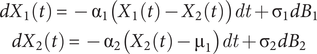 $$ {\displaystyle \begin{array}{c}d{X}_1(t)=-{\unicode{x03B1}}_1({X}_1(t)-{X}_2(t)) dt+{\unicode{x03C3}}_1d{B}_1\\ {}d{X}_2(t)=-{\unicode{x03B1}}_2({X}_2(t)-{\unicode{x03BC}}_1) dt+{\unicode{x03C3}}_2d{B}_2\end{array}} $$
These basic equations are generalized as a vector process to join any number of processes. Equation 4 of Reitan et al. (Reference Reitan, Schweder and Henderiks2012) shows this explicitly,
 $$ d\boldsymbol{X}(t)=(\boldsymbol{m}(t)+\boldsymbol{AX}(t)) dt+\boldsymbol{\Sigma} d\boldsymbol{B}(t) $$
where $ \boldsymbol{X} $
is a vector of processes,
$ \boldsymbol{X} $
is a vector of processes, $ \boldsymbol{m} $
is a deterministic component (e.g., equilibrium states),
$ \boldsymbol{m} $
is a deterministic component (e.g., equilibrium states), $ \boldsymbol{A} $
is a matrix of all the interactions of the processes,
$ \boldsymbol{A} $
is a matrix of all the interactions of the processes, $ \boldsymbol{\Sigma} $
is a matrix describing the covariance structure, and
$ \boldsymbol{\Sigma} $
is a matrix describing the covariance structure, and $ \boldsymbol{B} $
is multidimensional Brownian motion.
$ \boldsymbol{B} $
is multidimensional Brownian motion.
The components of $ \boldsymbol{X} $
can be evolutionary time series for multiple taxa with biotic interactions, in multiple geographic locations, and with environmental covariates. In the case of predator–prey coevolutionary alternation, necessary components would include time series for two prey species (at a minimum) and at least one predator. According to Thompson’s (Reference Thompson1994, Reference Thompson2005) hypothesis of coevolutionary alternation, the prey would gain defenses when being attacked and would lose defenses when not attacked. Thus, for each prey, we would include one or more time series of defensive traits (e.g., shell thickness or cost:benefit ratio, in the case of bivalves attacked by shell-drilling gastropods). Because the predator should have genetic preferences for the least-defended prey (Thompson Reference Thompson1999a, Reference Thompson2005), rather than simply consuming prey as encountered, predator preferences would also evolve as relative levels of defense change. Thus, one must include a time series of predator preference, for instance, using an electivity index (which measures feeding preference relative to the proportion of food types in the environment; Lechowicz Reference Lechowicz1982; Smith et al. Reference Smith, Handley and Dietl2018), to test for interactions with time series for the prey defensive traits.
$ \boldsymbol{X} $
can be evolutionary time series for multiple taxa with biotic interactions, in multiple geographic locations, and with environmental covariates. In the case of predator–prey coevolutionary alternation, necessary components would include time series for two prey species (at a minimum) and at least one predator. According to Thompson’s (Reference Thompson1994, Reference Thompson2005) hypothesis of coevolutionary alternation, the prey would gain defenses when being attacked and would lose defenses when not attacked. Thus, for each prey, we would include one or more time series of defensive traits (e.g., shell thickness or cost:benefit ratio, in the case of bivalves attacked by shell-drilling gastropods). Because the predator should have genetic preferences for the least-defended prey (Thompson Reference Thompson1999a, Reference Thompson2005), rather than simply consuming prey as encountered, predator preferences would also evolve as relative levels of defense change. Thus, one must include a time series of predator preference, for instance, using an electivity index (which measures feeding preference relative to the proportion of food types in the environment; Lechowicz Reference Lechowicz1982; Smith et al. Reference Smith, Handley and Dietl2018), to test for interactions with time series for the prey defensive traits.
Coevolutionary alternation predicts that different populations across the geographic range of the interacting species will differ in whether predator and prey traits are matched, because some populations of a prey species will be in the process of gaining and others in the process of losing defenses. Because different patterns in prey preferences and prey defenses are expected among populations, geographic information must also be included explicitly in the deterministic component of the model. SDEs are able to accommodate such a geographic component; for example, Reitan et al. (Reference Reitan, Schweder and Henderiks2012) constructed a model for evolution of coccolith sizes in cores from six sites in different regions in the Atlantic, Pacific, and Indian Oceans, where each region was modeled independently but had a common component that captured the influence of global temperature. To make geographic relationships more explicit, Reitan et al. (Reference Reitan, Schweder and Henderiks2012: p. 1549) suggested a possible modification of their approach in which “geographic information could be incorporated by letting the correlation between sites depend on the distance between the sites, for example, in relation to ocean circulation.” In the case of coevolutionary alternation, one might argue that sites that are closer may have greater dependency than sites that are farther apart, perhaps due to greater similarity of the environment and/or greater connectivity of populations, a reasonable assumption given that studies have shown that dispersal can occur over relatively short distances; for example, ~50–150 km for Pacific coral populations (Treml et al. Reference Treml, Halpin, Urban and Pratson2008) and 10–100 km for various Caribbean reef fish (Cowen et al. Reference Cowen, Paris and Srinivasan2006).
In modeling coevolutionary alternation, we recommend including enabling factors of the environment that could affect the coevolutionary process (e.g., see Toju Reference Toju2011). For instance, in the case of shell-drilling predators and their prey, predator metabolism can be influenced by temperature; Ansell (Reference Ansell1982) reported that in laboratory experiments, higher temperatures corresponded to greater feeding rates in the naticid gastropod Polinices catena, which could result in greater opportunity for reciprocal adaptation (i.e., hotter hot spots in the geographic mosaic). Temperature and productivity may affect the capacity of prey to build thicker shells, as calcification is facilitated by warmer waters and high productivity (Graus Reference Graus1974; Vermeij Reference Vermeij1987; Kirby Reference Kirby2001). Proxies for these enabling factors and other environmental conditions could be included when modeling coevolutionary alternation within the SDE framework. SDEs readily incorporate environmental time series (Reitan et al. Reference Reitan, Schweder and Henderiks2012; Liow et al. Reference Liow, Reitan and Harnik2015; Hannisdal and Liow Reference Hannisdal and Liow2018).
We also suggest some extensions that could help account for sampling and other biases. In their study of bivalve and brachiopod diversification, Liow et al. (Reference Liow, Reitan and Harnik2015) included a time series for sampling rate of each taxon, derived from occurrence data in the Paleobiology Database from which parameters were estimated with a capture–recapture model. Their goal was to improve diversification estimates by accounting for variation in sampling, which was recognized as including geological processes (e.g., deposition and erosion), morphological and ecological characteristics (e.g., body size, shell durability, and abundance), and sampling effort. These three sets of factors related to sampling bias would also need to be accounted for in modeling coevolutionary alternation, as follows.
In terms of geological processes, time averaging, with its effects on stratigraphic resolution and precision of correlation, would need to be addressed. The potential problems that time averaging produces for modeling coevolutionary alternation are similar to those discussed by Tomašových et al. (Reference Tomašových, Dominici, Nawrot, Zuschin, Nawrot, Dominici, Tomašových and Zuschin2023) for the integration of fossil and ecological data, particularly issues of disparity of temporal scale or changes in scale. The reciprocal adaptation that characterizes coevolution is confined to hot spots, and Dietl and Kelley (Reference Dietl, Kelley, Kowalewski and Kelley2002) noted that hot and cold spots may fluctuate in space and time. If the temporal scale of time averaging is too great, the underlying geographic mosaic may shift during the interval of interest (i.e., hot spots of reciprocal adaptation may become cold spots that lack reciprocal adaptation, and vice versa); likewise, environmentally condensed sections, in which time averaging combines deposits from multiple habitats (Kidwell and Bosence Reference Kidwell, Bosence, Allison and Briggs1991), could mix the record of hot and cold spots. Such time averaging of hot and cold spots will blur the record of reciprocal adaptation, and the alternation process will not be discernible. Even within hot spots, changes in predator preferences and the gain and loss of defenses may be rendered undetectable if the temporal scale of time averaging exceeds the scale at which coevolutionary change occurs. (One exception might be if coevolutionary alternation with escalation occurs: ratcheting up of defenses could be more observable than fluctuating levels of defenses, as long as time averaging is not so great as to blur the directional shift in defense levels.) In addition, to test coevolutionary alternation, the geographic locations being analyzed need to have experienced the same degree of time averaging to permit comparison of coevolutionary dynamics in different populations.
Morphological and ecological factors could also affect the record of coevolutionary alternation, for instance, if different prey items in the predator’s diet had different preservation potentials or different potentials for preserving evidence of predation needed to analyze predator preference, for example, drill holes. Both life mode and skeletal durability, which is related to size, microstructure, ornamentation, and thickness (Kosnik et al. Reference Kosnik, Alroy, Behrensmeyer, Fürsich, Gastaldo, Kidwell, Kowalewski, Plotnick, Rogers and Wagner2011), could affect the representation of prey species in the assemblages of interest. Ideally, preservation potential would be accounted for when modeling coevolutionary alternation.
Sampling effort (including effects on sample size) is a potentially complicating factor that also should be accounted for in testing coevolutionary alternation. Generally, sample size effects arise in uncertainties of estimated parameters (more data yield narrower confidence regions for parameter estimates). Further issues occur for predation data (e.g., presence/absence or counts of drill holes). For instance, drilling frequencies, which have been used as a measure of predator preference (e.g., Kelley and Hansen Reference Kelley and Hansen1996; Chattopadhyay and Dutta Reference Chattopadhyay and Dutta2013), can be inflated if a small sample happens to include drilled specimens. In an extreme example, if one of two individuals comprising a sample contains a drill hole, a drilling frequency of 0.50 would result—a value unlikely to occur in a larger sample. Conversely, as noted by Smith et al. (Reference Smith, Handley and Dietl2022), an excess of zero counts for predation traces can be the result of sampling issues (not having a large enough sample to provide evidence of predation that actually occurred or not having a random sample) or a true ecological effect (not being “on the menu”). Clearly, the latter possibility is of interest when predator preferences evolve, as in the coevolutionary alternation model. A predator may eliminate from its diet a prey that gains defenses, in which case lack of evidence of predation would not simply be the result of sampling issues. Such scenarios should be accounted for in the statistical model for predator preference.
In addition, there are a few methodological issues in the current implementation of SDEs that need to be resolved to make this approach fully applicable to modeling coevolutionary alternation. These issues include the following: (1) Current SDE models are unable to address situations in which causal relationships among time series change significantly through time and in which strong nonlinearity exists (Hannisdal and Liow Reference Hannisdal and Liow2018). However, Hannisdal and Liow (2015: p. 497) noted: “In a system where components are interdependent, such as ecosystems…, variables can interact in such a way that any linear correlations between them can change as the state of the system changes…. Even the simplest mathematical relations between two species can yield highly complex, nonlinear and unpredictable dynamics.” Given the complexities of the coevolutionary alternation process, changing and nonlinear causal relationships may be expected (e.g., in the shape of trade-off curves between prey growth and defense; Huang et al. Reference Huang, Traulsen, Werner, Hiltunen and Becks2017). (2) Distributional assumptions need to be relaxed to incorporate time series related to predation data, which typically are represented as presence/absence, counts, or proportions that are nonnormally distributed and are not readily transformed. To incorporate such data, one would need to generalize the SDE framework, which assumes normal distributions. Reitan and Liow (Reference Reitan and Liow2019: p. 2187) stated that these types of nonnormal data could be handled through generalized linear models, which are already commonly applied to predation data (e.g., Chattopadhyay et al. Reference Chattopadhyay, Zuschin and Tomašových2016). (3) The ability to handle many time series efficiently needs to be improved. Hannisdal and Liow (Reference Hannisdal and Liow2018: p. 500) noted that applying SDEs to systems with more than three time series can be expensive computationally, but in modeling coevolutionary alternation, we anticipate including traits of multiple prey species, prey preference of the predator(s), metrics related to sampling and other biases, and multiple environmental proxies (e.g., temperature and productivity). In suggesting this approach, we recognize the challenges involved and acknowledge that we may need to start with less complex models, perhaps with fewer time series. However, we believe that the approach can be applied fruitfully to modeling coevolution and investigating causes for stasis in the fossil record in traits relevant to biotic interactions.
Concluding Remarks
The original formulation of punctuated equilibria disregarded biotic interactions as important in evolution; within-species changes that might result from interactions were considered unimportant, because most evolution occurred at speciation. The common (perhaps dominant) pattern of stasis within species was thought to preclude processes such as coevolution, which was assumed to produce directional trends in interacting species.
During the past 50 years, many causes of stasis have been proposed with varying degrees of support, including explanations that stress biotic interactions and coevolutionary selection (e.g., Barnard Reference Barnard1984; Nordbotten and Stenseth Reference Nordbotten and Stenseth2016). In our judgment, one of the most promising is based on Thompson’s (Reference Thompson1994, Reference Thompson1999a, Reference Thompson2005) GMTC. As argued by Eldredge et al. (Reference Eldredge, Thompson, Brakefield, Gavrilets, Jablonski, Jackson, Lenski, Lieberman, McPeek and Miller2005), the geographic structure of populations experiencing different environmental pressures and coevolutionary dynamics can yield stasis on the scale of entire species. Among the specific hypotheses of the GMTC, coevolutionary alternation, with its expectations of different patterns of predator preferences and prey defenses within different populations and alternation of high and low levels of defense as predator preferences evolve, is a potentially powerful explanation of stasis within species in traits relevant to biotic interactions, such as predation. As we noted previously (Dietl and Kelley Reference Dietl, Kelley, Kowalewski and Kelley2002: p. 366), the fossil record provides strong support for spatial variation in predation pressure, which “sets up the conditions for a possible selection mosaic of hot and cold spots that have fluctuated in both space and time.”
Few studies have explicitly tested coevolutionary alternation (Chaves-Campos et al. Reference Chaves-Campos, Johnson and Hulsey2011), although quantitative coevolutionary models support its plausibility (Nuismer and Thompson Reference Nuismer and Thompson2006; Andreazzi et al. Reference Andreazzi, Thompson and Guimarães2017), and some results from modern communities are consistent with the hypothesis (e.g., Thompson Reference Thompson2005, Reference Thompson2009; Soler Reference Soler2014; Tartally et al. Reference Tartally, Thomas, Anton, Balletto, Barbero, Bonelli and Bräu2019). We realize that testing coevolutionary alternation in the fossil record is a challenging goal—not only in terms of the modeling approach but also because of the circumstances required to preserve a record of alternation. Like Liow et al. (Reference Liow, Uyeda and Hunt2023) and Kidwell and Holland (Reference Kidwell and Holland2002), we recognize the constraints on studying evolutionary processes that are imposed by the vagaries of the fossil record. Few paleontological studies have demonstrated disparate temporal patterns in local populations within spatially structured species, in part due to the challenges of conducting such work: studying multiple populations and localities from correlative strata with fine-scale time resolution. This perspective piece is a call for many more such studies in order to determine the plausibility of testing this idea and our working assumption that short-term eco-evolutionary dynamics indeed scale up (Aronson Reference Aronson1992; Thompson Reference Thompson1999b).
Thompson (Reference Thompson1994: p 268) stated: “Coevolutionary alternation … provides a clear view of how one species can coevolve with at least several other species, sometimes simultaneously and sometimes in an alternating sequence of recurring interactions that may take thousands of years to cycle.” Thus, in the fossil record, we may need to use “uncommonly studied time scales” (on the order of decades to millennia as represented by high-resolution environments) and “uncommonly studied organisms” (Liow et al. Reference Liow, Uyeda and Hunt2023: p. 258) instead of employing our favorite groups and stratigraphic sections (e.g., Maryland Miocene mollusks). Nevertheless, we anticipate that further development of the SDE approach to test coevolutionary alternation in appropriate settings may reveal coevolution as a viable cause of stasis in interacting species amid a constantly changing environment. Regardless of whether the specific hypothesis of coevolutionary alternation or even the more general GMTC is supported, we suspect that persistent coevolving interactions in communities will prevail as viable causes of stasis—and (contra Gould) demonstrate that ecology does matter in evolution.
Acknowledgments
This paper was initiated as a contribution to the 2022 Topical Session on “Punctuated Equilibrium: 50 Years Later” at the Geological Society of America annual meeting. We thank session co-organizers L. Ivany, B. Lieberman, D. Prothero, and M. Yacobucci for welcoming our contribution and the Paleobiology editors, especially J. Crampton, for being receptive to a special issue. B. Lieberman served as associate editor and E. Saupe as editor for this article, and we appreciate their guidance, as well as the comments of G. Hunt and an anonymous reviewer that improved the article.
Competing interests
The authors declare no competing interests.

 Open access