


Introduction
Evolutionary time series of populations in the fossil record provide information on phenotypic change on time intervals in between generational and macroevolutionary timescales. Analyses of these types of data are thus poised to make important contributions to our current understanding of evolution across the timescale continuum. For more than 15 years, Hunt's paleoTS framework (Hunt Reference Hunt2006, Reference Hunt, Kelley and Bambach2008a, Reference Huntb; Hunt et al. Reference Hunt, Bell and Travis2008, Reference Hunt, Hopkins and Lidgard2015; Hunt and Carrano Reference Hunt and Carrano2010) has been instrumental in generating new knowledge of evolutionary trait dynamics at the intersection between paleontology and evolutionary biology analyzing such time series. For example, trait evolution within lineages in the fossil record has been shown to be much more diverse than stasis alone (Hunt Reference Hunt2007; Hopkins and Lidgard Reference Hopkins and Lidgard2012; Hunt et al. Reference Hunt, Hopkins and Lidgard2015); microevolutionary parameters have been successfully estimated from fossil data (Hunt et al. Reference Hunt, Bell and Travis2008); and rates of evolution can be estimated using similar models, as in phylogenetic comparative methods (Hunt Reference Hunt2012). The new insights into phenotypic evolution provided by the paleoTS framework have thus contributed to a closer integration of paleontology and evolutionary biology.
Despite its success and impact, an extension of the paleoTS framework may be useful. First, a common use of the paleoTS R package is to investigate the relative fit of the three canonical models——stasis, unbiased random walk, and trend (modeled as an biased random walk)——to fossil time series. These models have a long history within paleontology (e.g., Raup Reference Raup and Hallam1977; Roopnarine Reference Roopnarine2001; Sheets and Mitchell Reference Sheets and Mitchell2001) but are not always able to adequately capture trait dynamics within lineages in the fossil record (Voje Reference Voje2018; Voje et al. Reference Voje, Starrfelt and Liow2018). Fitting and comparing a larger range of evolutionary models may enable a richer interpretation of evolutionary change within lineages (Fig. 1).

Figure 1. Univariate evolution models that can be fit and compared in evoTS. The models stasis, strict stasis, biased and unbiased random walk, and Ornstein-Uhlenbeck (OU) with fixed optimum are implemented in paleoTS (Hunt Reference Hunt2006; Hunt et al. Reference Hunt, Bell and Travis2008, Reference Hunt, Hopkins and Lidgard2015). The other models are implemented in evoTS. All models can be fit and compared in evoTS. In the OU model with a moving optimum, the population is either displaced from the optimum at the start of the sequence or is residing on or very close to the optimum (latter model indicated by *). The dotted horizontal line shows the position of the optimum in the OU model with a fixed optimum and the starting value of the optimum for the model where the optimum is allowed to change.
Second, the adaptive landscape has been suggested as a conceptual bridge between our understanding of microevolutionary processes and evolution observed across longer timescales (Simpson Reference Simpson1944; Arnold et al. Reference Arnold, Pfrender and Jones2001; Hansen Reference Hansen, Svensson and Calsbeek2012). However, knowledge of the dynamics of the adaptive landscape across time is poor. Macroevolution is likely associated with movements of peaks on the adaptive landscape, but a fixed adaptive landscape is commonly assumed in microevolutionary studies, which is also the case for the models implemented in paleoTS. Inferring the dynamics of the adaptive landscape from evolutionary time series may contribute to a better understanding of the dynamic nature of peak movements at different time intervals.
Third, evolution is inherently a multivariate phenomenon. Pleiotropy is omnipresent (e.g., Walsh and Blows Reference Walsh and Blows2009) and selection on one trait may cause genetically linked traits to evolve (Lande Reference Lande1979; Lande and Arnold Reference Lande and Arnold1983). Traits may also commonly experience correlated selection. Multivariate models are useful for investigating whether traits change in a correlated or uncorrelated manner, whether one trait/variable affects the optimum of a second trait, or whether adaptation in traits happens independently. The univariate models in paleoTS are of limited use for assessing the consequences of the multivariate nature of selection and evolution within lineages.
Here, I explore these three avenues of research by fitting uni- and multivariate models to examine evolution of size in a radiolarian lineage and multivariate evolution of armor traits in a stickleback lineage. Analyses employ the new R package, evoTS. As the univariate models in evoTS are natural extensions and modifications of the models in paleoTS, I start by introducing the univariate models available in paleoTS before I explain the expanded univariate models implemented in evoTS. I then apply these models to a well-known and previously published dataset, the evolution of size in the radiolarian lineage Eucyrtidium calvertense during allopatry and in a subsequent phase of neosympatry with its sister lineage Eucyrtidium matuyamai (Kellogg Reference Kellogg1975). I continue by introducing the multivariate models implemented in evoTS before I apply them in a reanalysis of a published dataset of two armor traits in a stickleback lineage (Bell et al. Reference Bell, Travis and Blouw2006; Hunt et al. Reference Hunt, Bell and Travis2008).
evoTS Is Compatible with paleoTS
I have developed evoTS to mirror the user experience from paleoTS as much as possible. The two frameworks use the same data format and the model-fitting procedures are built on the same assumptions. For example, all models assume the population (sample) means in the sequence of ancestor–descendants have a joint distribution that is multivariate normal with an expected mean vector and covariance matrix that are functions of the parameters of each model, the time intervals separating the populations (samples) in the sequence, and the sampling variances of the trait means calculated for each population (sample). The expected distribution of sample means is thus defined by their means, variances, and covariances given the assumption of multivariate normality. All models in evoTS have been implemented using the joint parameterization routine from paleoTS (Hunt Reference Hunt, Kelley and Bambach2008a), with the autocorrelation among samples being accounted for in the log-likelihood function. As in the paleoTS package, evoTS uses a quasi-Newton optimization routine for estimating maximum likelihood parameter estimates for univariate models, while the Nelder-Mead hill climbing algorithm is the default option for some of the multivariate models. Relative model fit is evaluated based on the small sample-corrected version of the Akaike information criterion (AICc) (Akaike Reference Akaike1974; Burnham and Anderson Reference Burnham and Anderson2002).
Univariate Models in paleoTS
Unbiased random walk, biased random walk (trend model), and stasis were the first models implemented in the paleoTS framework (Hunt Reference Hunt2006). An unbiased random walk models evolution of a trait mean as independent draws from a normal distribution with mean zero (μ = 0) and a variance  $\rm ( {\sigma_{step}^2 } ) $ commonly referred to as the step variance (Hunt Reference Hunt2006). Each draw represents a discrete evolutionary “step,” and the expected amount of evolution in the trait mean z per time step i is 0.
 $$E[ {z_i} ] = z_0$$
The trait mean is therefore not expected to be different from the ancestral state z 0, but the variance around this expectation increases linearly with elapsed time,
 $${\rm Var}[ {z_i} ] = \rm \sigma _{step}^2 \it t_i + {\rm \varepsilon} _i$$
where ti is the elapsed time from the start of the time series to sample i (time at the start of the time series is always 0). The variance in each sample is influenced by the sampling error  $( {\rm \varepsilon}_{i} ) $ in estimating the trait mean, which is equal to the sample variance divided by the sample size (i.e., number of measured specimens) for that sample. The covariance among sample means is given by:
 $${\rm Cov}[ {z_i, \;z_j} ] = \rm \sigma _{step}^2 {\it t_{\min }}$$
where t min represents the time interval between the start of the sequence and the earliest of the samples zi and zj.
The biased random walk (sometimes referred to as a trend model; e.g., see Hansen [1997]) is identical to an unbiased random walk except for a nonzero mean (μ ≠ 0) of the normal distribution from which evolutionary steps are drawn (Hunt Reference Hunt2006). A larger deviation from 0 of the mean translates into a stronger tendency to change unidirectionally in trait space. The expressions for the variance and covariance are identical for the biased and unbiased random walk (eqs. 2 and 3), while the expected mean trait value is given by:
 $$E[ {z_i} ] = z_o + {\rm \mu} t_i$$
Various definitions of stasis have been employed in research that aims to quantify change in evolutionary time series (e.g., Bookstein Reference Bookstein1987; Gingerich Reference Gingerich1993; Roopnarine Reference Roopnarine2001; Sheets and Mitchell Reference Sheets and Mitchell2001). The stasis model in paleoTS is similar to a white noise process where trait evolution consists of uncorrelated fluctuations around a fixed trait value (θ) (Hunt Reference Hunt2006). The fluctuations around the fixed mean are described by a variance parameter (ω), which is assumed to stay constant over time. Time is accordingly not a relevant parameter in the stasis model. The strict stasis model (Hunt et al. Reference Hunt, Hopkins and Lidgard2015) is identical to the previously described stasis model, except that ω = 0, which can be the case when the variance among trait means is smaller than the sampling error in the trait means, that is, the observed differences among trait means can be explained by sampling error alone (see also Hannisdal Reference Hannisdal2006).
Hunt et al. (Reference Hunt, Bell and Travis2008) extended the paleoTS framework with the implementation of an Ornstein-Uhlenbeck (OU) model describing evolution of a trait toward a fixed peak in the adaptive landscape (Hansen Reference Hansen1997). The OU process is the simplest stochastic model that allows evolution toward a specific state and is given by the following differential equation:
 $$dy = {\rm \alpha} ( {\rm \theta -\it y} ) dt + {\rm \sigma} _ydW_y$$
where dy is the change in the trait (y) over a time step dt, α describes the rate of evolution toward the optimum θ, dW y represents independent and normally distributed changes with mean 0 and unit variance, with σy being the standard deviation of this white noise process. The first part of the OU process is deterministic and describes how the trait is pulled toward the optimum at a rate given by α. The second part is a stochastic process adding random noise scaled by the σy parameter to the trait dynamics. The expected change in a trait mean z per time step i and its variance and covariance are given by:
 $$E[ {z_i} ] = e^{( {-\rm \alpha \it t_i} ) }z_0 + [ {1-e^{( {-{\rm \alpha} t_i} ) }} ] {\rm \theta }$$
 $${\rm Var}[ {z_i} ] = ( {\rm \sigma_{step}^2 /2\alpha } ) [ {1-e^{( {-2{\rm \alpha} t_i} ) }} ] + {\rm \varepsilon} _i$$
 $${\rm Cov}[ {z_i, \;z_j} ] = ( {\rm \sigma_{step}^2 /2\alpha } ) e^{( {-{\rm \alpha} t_{ij}} ) }[ {1-e^{( {-2{\rm \alpha} t_{\rm min}} ) }} ] $$
where θ is the optimal trait value and t ij is the time separating samples i and j (Hansen Reference Hansen1997; Hunt et al. Reference Hunt, Bell and Travis2008).
Univariate Models in evoTS
Simple models often sacrifice precision and nuance to distill general properties from data (Levins Reference R1966). An evolutionary time series showing a relative better fit to an unbiased random walk compared with a stasis model does not mean trait evolution was random in each generation in the analyzed lineage. Rather, it suggests that the observed trait dynamics are more consistent with a pattern of “meandering” evolution, in which random changes in the trait mean accumulate over time, rather than with random fluctuations around a constant mean (akin to a white noise process). Adding or changing a few parameters in the models implemented in paleoTS can aid in extracting additional information not captured by the original models.
In the following sections, I describe the univariate models implemented in evoTS and briefly discuss how they can be interpreted when fit to evolutionary sequences. evoTS is available for download from the Comprehensive R Archive Network (CRAN) (http://cran.r-project.org). The online vignette contains a detailed walk-through that explains from a user perspective how to fit all the different univariate models in evoTS (and paleoTS) and how to evaluate their relative fit to data (klvoje.github.io/evoTS/index.html).
Time-Varying Unbiased Random Walks
The rate of evolution is constant in an unbiased random walk, which means the trait variance is expected to increase linearly with time. A natural extension of this model is to allow the rate of evolution to change with time. The decelerated model of evolution implemented in evoTS is an unbiased random walk where the net rate of change declines exponentially through time. This model is basically identical to the early burst model developed for phylogenetic comparative data to test for a decelerated rate of evolution at the clade level (e.g., Cooper and Purvis Reference Cooper and Purvis2010; Harmon et al. Reference Harmon, Losos, Davies, Gillespie, Gittleman, Jennings, Kozak, McPeek, Moreno-Roark, Near, Purvis, Ricklefs, Schluter, Schulte, Seehausen, Sidlauskas, Torres-Carvajal, Weir and Mooers2010). The expected evolutionary divergence between ancestor and descendant populations is zero in the decelerated evolution model (eq. 1) and its variance and covariance are given by:
 $${\rm Var}[ {z_i} ] = { \sigma }_{{\rm step}.0}^2 { (e^{rt_{i}}-1) \over r } + \rm \varepsilon _ {\it i}$$
 $${\rm Cov}[{z_i, \;z_j} = {\rm \sigma}_{{\rm step}.0}^2 {( e^{rt_{\rm min}}-1)} \over {r}$$
where σ2step.0 is the initial value for the step distribution, and r describes the exponential decay in the rate change through time and is thus constrained to be < 0 (Harmon et al. Reference Harmon, Losos, Davies, Gillespie, Gittleman, Jennings, Kozak, McPeek, Moreno-Roark, Near, Purvis, Ricklefs, Schluter, Schulte, Seehausen, Sidlauskas, Torres-Carvajal, Weir and Mooers2010). An accelerating model of evolution is identical to the decelerated model, except that the r parameter is constrained to be > 0. The time it takes to halve (for the decelerated evolution model) or double (for the accelerated evolution model) the rate of evolution is given by ln(2)/|r|. The estimating algorithm in evoTS generally produces precise estimates of the r parameter in the decelerated and accelerated models (more details are given in Supplementary Fig. 1).
Model Interpretation
A linearly increasing trait divergence with time will rapidly produce magnitudes of evolutionary change rarely observed in nature (e.g., Lynch Reference Lynch1990; Gingerich Reference Gingerich2001; Estes and Arnold Reference Estes and Arnold2007; Uyeda et al. Reference Uyeda, Hansen, Arnold and Pienaar2011). A decelerating rate of evolution mitigates this problem. Although many evolutionary scenarios and processes can be compatible with unbiased random walk models, a decrease in the rate of evolution over time might occur, for example, when a lineage experiences less selection after a period of higher initial rates of evolution due to changes in the environmental conditions (e.g., Voje Reference Voje2020). A reduced rate may also occur if the effect of drift is reduced over time (i.e., due to increasing population size). An accelerated rate of evolution is not sustainable across long timescales but might fit lineages that experience an increased effect of drift or increasing environmental perturbations. Note that interpreting the trait dynamics as the results of neutral drift only may not be a plausible interpretation for ecologically relevant traits across long timescales (e.g., Hansen Reference Hansen, Svensson and Calsbeek2012). An alternative—and perhaps more likely—interpretation of unbiased random walk models is that they provide information on peak movements of the adaptive landscape. This is indeed a common interpretation of the related Brownian motion model in phylogenetic comparative approaches (Felsenstein Reference Felsenstein1988). As long as populations are sufficiently evolvable to immediately track changes in the locations of peaks in the adaptive landscape, the step variance ( ${\rm \sigma }_{{\rm step}}^2 $) provides insight on the rate of change of the adaptive peak itself according to this interpretation of the model. The decelerated and accelerated models may therefore represent scenarios where the rate of peak movements changes with time.
OU Models with Moving Optimum
A natural extension of the fixed-peak OU model implemented in paleoTS is to allow the peak to change. A model where the optimum is changing according to Brownian motion was proposed by Hansen et al. (Reference Hansen, Pienaar and Orzack2008) for analysis of phylogenetic comparative data. Adjusted to describe evolution of a single lineage, the expected trait mean is given by equation (6), while the variance and covariance are given by the following expressions:
 $$\eqalign{{\rm Var}[ {z_i} ] & = \left[{\displaystyle{{\rm \sigma_{step}^2 + \sigma_\theta^2 } \over {2\rm \alpha }}} \right][ {1-e^{( {-2{\rm \alpha} t_i} ) }} ] \cr & \quad + {\rm \sigma }_{\rm \theta }^2 t_i[ {1-2( {1-e^{-{\rm \alpha} t_i}} ) /{\rm \alpha} t_i} ] \cr & \quad + {\rm \varepsilon} _{\rm min}}$$
 $$ \eqalign{& {\rm Cov}[ {z_i, \;z_j} ] = \left[{\displaystyle{{\rm \sigma_{step}^2 + \sigma_\theta^2 } \over {2\rm \alpha }}} \right][ {1-e^{( {-2{\rm \alpha} t_{\rm min} } ) }} ] e^{-{\rm \alpha} t_{ij}} \cr & \quad + {\rm \sigma }_{\rm \theta }^2 t_{\rm min} [ {1-( {1 + e^{ - {\rm \alpha} t_{ij}}} ) ( {1-e^{-{\rm \alpha} t_{\rm min} }} ) /{\rm \alpha}} t_{\rm min} ]}$$
where θ0 is the initial (ancestral) optimum, σ2θ is the (step) variance of the stochastic perturbations of the optimum. The half-life, ln(2)/α, is a reparameterization of the speed of adaptation in this process that is easy to interpret, as it is the time it takes for the trait to move halfway from the ancestral state to the optimum. The estimation algorithm is able to identify model parameters well, but outliers occur. Precision increases with longer time series (see Supplementary Fig. 2 for more details).
Model Interpretations
The stability of the adaptive landscape is debated and is likely affected by many factors (e.g., Slater and Friscia Reference Slater and Friscia2019). A lineage in a hyper-stable niche may reside on a fixed peak, while a lineage inhabiting a more unstable environment may experience a more dynamic adaptive landscape. For example, traits with specialized ecological roles insensitive to changes in overall size (i.e., allometry) may reside on stable peaks, while the peak of a size-associated trait easily affected by changing ecological conditions may be in constant flux. Being able to explicitly test whether a fixed or a dynamic optimum model best fit a given evolutionary sequence may provide a valuable perspective on the dynamic nature of the adaptive landscape.
Mode-Shift Models
There is no a priori reason why a lineage should be described by a single evolutionary process (Hunt Reference Hunt2008b; Hunt et al. Reference Hunt, Hopkins and Lidgard2015). Mode-shift models allow two or more separate segments of a time series to evolve according to different models. evoTS includes a function that enables the testing of all possible pairwise combinations of four models: unbiased random walk, biased random walk, stasis, and OU. This function also allows for the independent parameterization of the same model for two separate segments. In addition to assessing all possible switch points in mode of evolution, it is also possible to define where in the sequence a shift in mode occurs, a helpful feature if we have an a priori hypothesis for when a shift happened.
Applying the Univariate Models
Changes in the adaptive landscape may affect how lineages evolve. I reinvestigate an evolutionary sequence of a radiolarian lineage to assess the dynamics of the adaptive landscape across a few million years and whether it affects size change in the lineage.
Background
Kellogg (Reference Kellogg1975) investigated whether size evolution in the radiolarian lineage Eucyrtidium calvertense showed trait dynamics consistent with a scenario of character displacement (Fig. 2). Eucyrtidium matuyamai evolved from E. calvertense in subarctic waters, and the two lineages differentiated during a period of allopatry. The two species came into secondary contact when a population of E. matuyamai migrated to subtropical waters. During this neosympatric phase, the two lineages differentiated in size, with E. matuyamai evolving to become about 25% larger and E. calvertense to become about 10% smaller. Kellogg (Reference Kellogg1975) concluded that the evolutionary sequence of E. calvertense in subtropical waters showed little net change during the allopatric phase, but a trend toward smaller size in the neosympatric phase, a type of trait dynamics Kellogg (Reference Kellogg1975) interpreted to be consistent with the process of character displacement. The evolutionary sequence spans 3.67 Myr and consists of 49 samples with median and mean numbers of measured specimens per sample of 25 and 25.4, respectively (Fig. 2). The allopatric and neosympatric phases last for about 1.70 and 1.97 Myr, respectively.

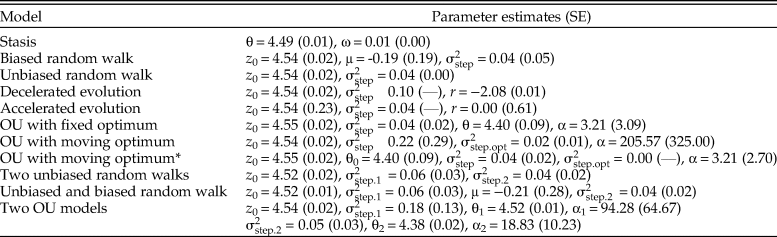
Figure 2. Size evolution in Eucyrtidium calvertense (Kellogg Reference Kellogg1975). The vertical gray bar indicates the shift from allopatry to sympatry with Eucyrtidium matuyamai. Blue dots belong to the allopatric phase, and orange points belong to the sympatric phase. The best model is a mode-shift model consisting of two Ornstein-Uhlenbeck (OU) processes with fixed optima. The maximum likelihood parameter estimates (±SE) of this model are: z 0 = 4.543 (±0.019), θ1 = 4.524 (±0.009), θ2 = 4.377 (±0.021),  ${\rm \sigma }_{{\rm step}.1{\rm \;}}^2 = $ 0.183 (±0.130), ${\rm \sigma }_{{\rm step}.2{\rm \;}}^2 = $ 0.046 (±0.027), α1 = 94.282 (±64.671), α2 = 18.833 (±10.231). The broken horizontal lines represent the fixed optimal trait values from the OU–OU model.
Fitted Models
A mode-shift model consisting of two OU models (i.e., an OU–OU model) can assess whether the initiation of the neosympatric phase led to a sudden change in the position of the adaptive peak for size in E. calvertense. I also fit OU processes with a constantly changing optimum to investigate how well models assuming continuous change of the adaptive landscape explained the data. To investigate whether models assuming a fixed adaptive landscape outcompeted the models assuming a dynamic landscape, I fit the stasis model, the trend model (i.e., a biased random walk), and unbiased random walk model with fixed, decelerating, and accelerating rates of evolution, and mode-shift models where the allopatric and neosympatric parts were either modeled as two unbiased random walks or where the second model was a biased random walk. Data and R scripts for replicating the analyses are available in the Supplementary Material.
Results
The OU–OU mode-shift model showed the best relative fit to the data (Table 1), with an optimal trait value during the sympatric phase (4.38 log micrometer) that was 13% smaller compared with the optimum during the sympatric phase (4.52 log micrometer). The adaptive process is faster in the allopatric phase (ln(2)/α = 0.007, which translates into a half-life of about 27,000 years) compared with the sympatric phase (ln(2)/α = 0.037, i.e., a half-life of about 135,000 years; Table 2). The log-likelihood surfaces of the half-life values show some overlap in the two phases (Fig. 3), but while a half-life of 4.05% (about 150,000 years) of the sequence length is within 2 log-likelihood units in the allopatric phase, the equivalent value of the second phase is 31.51% (about 1,160,000 years). The stochastic part of the trait dynamics is also elevated during the allopatric phase ( ${\rm \sigma }_{{\rm step}.1{\rm \;}}^2 $= 0.183) compared with the sympatric phase ( ${\rm \sigma }_{{\rm step}.2{\rm \;}}^2 $ = 0.046). To investigate whether the difference in temporal resolution between the two segments could explain the difference in trait dynamics, I subsampled the first segment 1000 times to match the length of the second segment (14 samples) and re-estimated the half-life and ${\rm \sigma }_{{\rm step\;}}^2 $ parameters. The median estimates of the half-life and ${\rm \sigma }_{{\rm step\;}}^2 $ from the subsampled data were 0.010 and 0.111, which suggests that differences in temporal resolution alone cannot explain the difference in the estimated trait dynamics between the two segments. The allopatric phase therefore appears to be characterized by faster evolution toward the fixed optimum and larger stochastic deviations from the optimum compared with the sympatric phase.

Figure 3. Log-likelihood surfaces for the Ornstein-Uhlenbeck (OU–OU) model. The panels show the support surface for the OU model describing the evolutionary sequence before and after the mode shift, respectively. The elevated area represents parameter estimates that are within two log-likelihood units of the best estimate. A, The first part of the sequence; the two-unit support surface includes immediate adaptation (i.e., half-life = 0) and extends up to 0.040. B, The second part of the sequence where a half-life of zero is not part of the support surface (0.019–0.315). The ranges of support for the two stationary variances are 0.000–0.002 and 0.001–0.008. Note that these results are conditional on the best estimate of the other parameters in the model (i.e., the ancestral state and the optimum).
Table 1. Model fit to the Eucyrtidium calvertense sequence. The log-likelihood (log-lik.) and the relative model fit for the candidate models fit to the evolutionary sequence of E. calvertense. OU, Ornstein-Uhlenbeck; K, number of parameters in model; AICc, Akaike information criterion corrected for small sample size; *, the population at the start of the sequence is residing on or very close to the optimum.

Table 2. Maximum likelihood parameter estimates for the candidate models fit to the Eucyrtidium calvertense sequence. See equations and main text for definitions of the different model parameters. The numbers in parentheses are standard errors calculated from the square root of the inverse of the diagonal of the Hessian matrix. OU, Ornstein-Uhlenbeck; *, the population at the start of the sequence is residing on or very close to the optimum.
Models that differ in their relative model fit by a few AICc units may be worth considering as plausible or suitable alternative explanations of an empirical dataset (Burnham et al. Reference Burnham, Anderson and Huyvaert2011). The OU model with a constantly changing optimum has a very similar fit compared with the best model (ΔAICc = 0.412). The alpha parameter describing the rate of evolution toward the moving optimum is large (205.57), translating into a point estimate of the half-life of about 10,000 years. The point estimate of the rate of change in the optimum ( ${\rm \sigma }_{{\rm step}.{\rm opt\;}}^2 = 0.02) \;$ indicates a non-fixed optimum through time. The stochastic part of the trait dynamics is rather large ( ${\rm \sigma }_{{\rm step}}^2 $= 0.22), suggesting size evolution in E. calvertense has contributions from both the deterministic and stochastic part of the OU model. A reasonable interpretation of the trait dynamics in E. calvertense according to the parameter values of this OU model is as a white noise process around a stochastically moving peak. Note that both the unbiased random walk and the decelerating unbiased random walk show a similar, albeit somewhat poorer, fit to the data compared with the OU process with a moving optimum. This is not surprising, as the optimum in the OU process changes according to an unbiased random walk. The better fit of the OU model is due to the size of the fluctuations around the optimum, which is sufficiently large not to be accounted for by measurement error in the samples. Not controlling for error in the samples would therefore unduly favor the unbiased random walk instead of the OU process.
In summary, the best model among the candidates suggests the position of the optimum changed toward a smaller optimal size when E. calvertense comes into secondary contact with E. matuyamai. Evolution toward a randomly changing optimum in both the allopatric and sympatric phases of the evolutionary sequence, or “meandering” evolution described by unbiased random walk models, are also likely models of the trait dynamics in E. calvertense.
Multivariate Models in evoTS
Much can be learned from studies of single traits, but a trait-by-trait approach has some important shortcomings. The omnipresence of pleiotropy suggests only a very small number of truly genetically independent traits exist (Barton Reference Barton1990; Johnson and Barton Reference Johnson and Barton2005; Walsh and Blows Reference Walsh and Blows2009). Evolutionary change in a trait is only rarely due to selection operating on that trait alone, as selection on genetically linked traits may also affect the focal trait (Lande Reference Lande1979; Lande and Arnold Reference Lande and Arnold1983; Hansen and Houle Reference Hansen and Houle2008). Traits that are genetically independent may still be functionally dependent, which means they may experience coordinated selection and therefore have a tendency to evolve in concert. Trait evolution is thus inherently a multivariate process that requires multivariate models to be more fully understood.
The following sections provide a description of the multivariate models available in evoTS and how they can be interpreted. The online vignette details from a user perspective how to fit the different multivariate models implemented in evoTS, including walk-throughs and examples of how to test different hypotheses of evolution and adaptation (klvoje.github.io/evoTS/index.html).
Multivariate Unbiased Random Walks
The multivariate unbiased random walk model can assess whether a set of traits evolve in a coordinated fashion or not. This is done by estimating an evolutionary rate matrix R (Felsenstein Reference Felsenstein2004; Revell and Harmon Reference Revell and Harmon2008; Revell and Collar Reference Revell and Collar2009). The R matrix describes the rate of evolution in the investigated traits on the diagonal (i.e., the diagonal contains the step variances) and the covariance of the changes in the traits in the off-diagonal elements. The multivariate variance–covariance matrix for the unbiased random walk model (V) is computed using the Kronecker product of the R matrix and a “distance matrix” C, describing how the different samples/populations are separated in time.
 $${\rm \bf V} = \mathop \sum \limits_{i = 1}^m {\rm \bf R}_{\boldsymbol i}\otimes {\rm \bf C}_{\boldsymbol i}$$
where m represents the number of non-overlapping segments of a time series that have their own R matrix. Sampling error of the trait mean (calculated as the sample variance divided by the sample size) is added to the diagonal of V. To ensure symmetric positive definiteness of the V matrix during log-likelihood optimization, R is parameterized by its Cholesky decomposition as the cross-product of upper triangular matrices:
 $${\rm \bf R} = {\rm \bf L}{\rm \bf L}^{\boldsymbol T}$$
where L is a square matrix with positive diagonal entries. L is upper triangular if there are off-diagonal elements in R. As for the univariate unbiased random walk, it is possible to test for a decrease or increase in the rate of change over time in the multivariate unbiased random walk model in evoTS. The r parameter adjusting the rate is assumed common for all the traits. Simulations show that the estimating procedure produces unbiased parameters even at sequence lengths of about 10 samples (see Supplementary Fig. 3 for more info).
Model Interpretation
Potential causes of correlated trait evolution are many. Traits may, for example, independently follow optima governed by the same environmental drivers, show concerted evolution due to shared direct or indirect selection, or be affected similarly by genetic drift.
Note that the R matrix is not the same as the genetic (G) or phenotypic (P) covariance matrices commonly estimated in quantitative genetics. However, the R matrix is connected to these matrices under certain assumptions. For example, the R matrix is expected to be proportional to the additive genetic variance–covariance matrix (G) if the traits evolve due to genetic drift only (Lande Reference Lande1979; Felsenstein Reference Felsenstein1988). Estimating R can thus aid in assessing to what extent evolution within lineages matches predictions from quantitative genetics.
Multivariate OU Models
Multivariate evolution is more than correlated change. Multivariate versions of the OU process allow for sophisticated investigations of a range of hypotheses regarding evolution and adaptation and are described by the following differential equation (Bartoszek et al. Reference Bartoszek, Pienaar, Mostad, Andersson and Hansen2012; Reitan et al. Reference Reitan, Schweder and Henderiks2012; Clavel et al. Reference Clavel, Escarguel and Merceron2015):
 $$dZ (t) = {\rm \bf A}[ {{\rm \bf \theta }( t ) -{\rm \bf Z}( t ) } ] dt + {\rm \bf R}dW(t)$$
where A is a square matrix (with dimensions equal to the number of traits) describing the rate of evolution toward the optimal trait values, θ is a vector containing the optimum for each trait, R is a square matrix (with dimensions equal to the number of investigated traits) describing the stochastic changes in the traits, and W is the diffusion parameter. Under the assumption that we only have one selective regime (optimum) per trait, the expected trait means of the OU process are the weighted sum of the optimum and the ancestral trait value (Hansen Reference Hansen1997):
 $$E[ {{\boldsymbol Z}_i } ] = e^{( {-{\boldsymbol A}t_i} ) }{\boldsymbol z}_0 + [ {1-e^{( {-{\boldsymbol A}t_i} ) }} ] {\rm \theta }$$
where Zi is a vector containing the expected trait values for sample i, z0 is a vector containing the ancestral trait means, and t i is the time interval from the ancestral population mean (the start of the time series, which has a time of 0) to the ith population mean.
The variance and covariance of sample/population means are given by the following expression (Bartoszek et al. Reference Bartoszek, Pienaar, Mostad, Andersson and Hansen2012; Reitan et al. Reference Reitan, Schweder and Henderiks2012; Clavel et al. Reference Clavel, Escarguel and Merceron2015):
 $$\eqalign{{\rm Cov}( {z_i, \;z_j} ) & = \left[{\bf Q}\left({\left\{{1 \over {\lambda_k + \lambda_l}}[1-e^{-(\lambda_k + \lambda_l) t_{\rm min}}]\right\}}_{1 \le k, l \le m}\right.\right. \cr & \quad \left.\left. {\odot \; {\bf Q}^{-1}{\bf L}{\bf L}^{\boldsymbol T}({\bf Q}^{-1})^T}\right){\bf Q}^T \right]e^{-{\boldsymbol A}^T t_{ij}}}$$
where Q is the orthogonal matrix of eigenvectors of A,  ${\rm \bf L}{\bf L}^{\boldsymbol T}$ is the Cholesky decomposition of the R matrix (R = ${\bf L}{\bf L}^{\boldsymbol T}$), λi is the ith eigenvalue of A, t min is the time interval between the start of the sequence and the earliest of the samples zi and zj, t ij is the time separating two samples zi and zj, and ⊙ represents the Hadamard (element-wise) matrix product. Under the assumption that the A matrix has a number of linear independent eigenvectors equal to the number of traits investigated, A can be expressed by its eigendecomposition:
 $${\bf A} = {\bf Q}\Lambda {\bf Q}^{{-}1}$$
where Λ is a matrix with the eigenvalues (λ) of A on the diagonal. The matrix exponential in equation (17) can then be solved using the eigendecomposition of A (Bartoszek et al. Reference Bartoszek, Pienaar, Mostad, Andersson and Hansen2012; Reitan et al. Reference Reitan, Schweder and Henderiks2012; Clavel et al. Reference Clavel, Escarguel and Merceron2015):
 $$e^{-{\boldsymbol A}t} = {\bf Q}{\rm diag}( {e^{-\lambda_1t}, \;\ldots , \;e^{-\lambda_mt\;}} ) {\bf Q}^{{-}1}$$
Precise estimation of parameters is a challenge that tends to increase with model complexity. Parameter estimation under univariate and multivariate phylogenetic OU models can be difficult (Hansen et al. Reference Hansen, Pienaar and Orzack2008; Bartoszek et al. Reference Bartoszek, Pienaar, Mostad, Andersson and Hansen2012, Reference Bartoszek, Gonzalez, Mitov, Pienaar, Piwczyński, Puchałka, Spalik and Voje2023; Ho and Ané Reference Ho and Ané2014; Cressler et al. Reference Cressler, Butler and King2015), but simulations show that multivariate OU model parameters in evoTS are overall identifiable. Precision is high for diagonal elements in R and A and the optima even for short time series. The median parameter estimate of the off-diagonal element in A is in the proximity of the true value for short sequence lengths and approaches the true value with increasing sequence lengths (see Supplementary Fig. 4 for more info).
Model Interpretation
The A and R matrices are key to defining the trait dynamics in a multivariate OU model. The elements in R control the stochastic parts of the trait dynamics in the OU process and can be interpreted similarly as R in the multivariate unbiased random walk: the diagonal elements in R represent the step distributions (step variances) of the changes in each individual trait, while any nonzero off-diagonal elements represent the covariance of the stochastic changes in the traits. The elements in the A matrix affect the deterministic part of the OU process, that is, the adaptive process of traits evolving toward optima. The diagonal elements in A are the individual alpha parameters for each trait, while a nonzero off-diagonal element reflects how changes in the trait affect the optimum of another trait. Four broad categories of hypotheses can be investigated based on how the A and R matrices are parameterized.
Independent Trait Evolution
Both the deterministic and stochastic parts of the evolutionary trait dynamic are independent for each trait. This model is the equivalent of fitting univariate OU models to each trait separately and is parameterized in the multivariate version by allowing only diagonal elements in the A and R matrices to be nonzero.
Independent Adaptation
Each trait adapts independently to its optimum, but the stochastic part of the trait dynamics is correlated. This model is obtained if the A matrix is diagonal while the R matrix has nonzero off-diagonal elements.
Non-independent Adaptation
Changes in trait X affect the optimum of trait Y, but changes in Y do not affect the optimum of trait X. A can be a nonsymmetric matrix (contrary to the R matrix), which means one trait is allowed to affect the optimum of another trait, but not vice versa. A negative number in an off-diagonal element in A means the trait is evolving toward the optimum, while a positive number means the trait is evolving away from the optimum. The stochastic changes in the trait (controlled by the parameterization of the R matrix) can be either correlated or uncorrelated.
Reciprocal Adaptation
Traits affect one another's optima. This is the case if their respective off-diagonal elements in A are nonzero. One trait may assert a larger effect on the optimum of another trait. The stochastic changes in the trait can be either correlated or noncorrelated.
An A matrix with nonzero off-diagonal elements investigates Granger causality between the traits/variables (Granger Reference Granger1969; Schweder Reference Schweder1970; Reitan et al. Reference Reitan, Schweder and Henderiks2012; Hannisdal and Liow Reference Hannisdal and Liow2018; Reitan and Liow Reference Reitan and Liow2019). Granger causality is a statistical concept that is used to determine whether one time series is useful in predicting another. Simply speaking, we have evidence for Granger causality if observations in one time series are useful for forecasting future observations in one or several other time series. The multivariate OU process therefore allows us to move beyond interpreting correlations among variables in time series. A correlation is symmetric (the correlation between X and Y is the same as the correlation between Y and X), but that is not needed for Granger causality. X can (Granger) cause Y, without Y Granger-causing X. Forecasting using Granger causality is only possible if there is some lag in the tracking of the optimum, that is, if a trait is unable to immediately respond to changes in the optimum. The rate of adaptation in the multivariate OU model is determined by the entries in the A matrix and can be conveniently calculated by the half-life. As in the univariate OU model, the half-life (ln(2)/αii) describes the time it takes for the trait to move halfway from the ancestral state to the new optimal state.
The multivariate OU model is reduced to an unbiased random walk if the diagonal elements in A are zero. Within the multivariate OU process, it is therefore possible to allow traits/variables that change according to an unbiased random walk to affect the optimum of traits evolving according to an OU process. Models with a mix of traits evolving as either OU or as an unbiased random walk have been termed “OUBM models” in the phylogenetic comparative literature (e.g., Bartoszek et al. Reference Bartoszek, Pienaar, Mostad, Andersson and Hansen2012, Reference Bartoszek, Gonzalez, Mitov, Pienaar, Piwczyński, Puchałka, Spalik and Voje2023). An OUBM model may, for example, be a sensible choice if we want to investigate whether an environmental variable (e.g., a paleoclimatic proxy) that we assume changes as an unbiased random walk affects the optimum of a trait we assume evolves according to an OU process.
Applying the Multivariate Models
Analyzing several traits or variables jointly using multivariate models enables a more sophisticated assessment of alternative hypotheses of the observed trait dynamics in the data relative to analyzing each trait separately. I apply multivariate models on a dataset on armor trait evolution in a threespine stickleback lineage (Gasterosteus doryssus) that has previously been analyzed using univariate models (Bell et al. Reference Bell, Travis and Blouw2006; Hunt et al. Reference Hunt, Bell and Travis2008). Strong genetic covariances among armor traits (Leinonen et al. Reference Leinonen, Cano and Merilä2011) and evidence that different armor traits are affected by the same loci (Cresko et al. Reference Cresko, Amores, Wilson, Murphy, Currey, Phillips, Bell, Kimmel and Postlethwait2004) in extant threespine sticklebacks (Gasterosteus aculeatus) suggest armor traits may not evolve independently. Armor traits are also likely to serve similar ecological functions and may therefore often experience similar selection pressures. A multivariate approach is therefore warranted when analyzing armor traits in threespine sticklebacks.
Background
Bell et al. (Reference Bell, Travis and Blouw2006) analyzed morphological evolution in three skeletal traits in a fossil stickleback lineage (G. doryssus) across more than 7000 years from well-preserved lake sediments. The three traits are part of the armor of the fish: number of dorsal spines, number of touching pterygiophores, and a pelvic trait measured based on scores of the completeness of the pelvic condition. All three traits show a clear trend of reduction in number (and score) during the time series, likely as a consequence of a reduced predation pressure in the lake (Bell et al. Reference Bell, Travis and Blouw2006). However, Bell et al. (Reference Bell, Travis and Blouw2006) did not find strong evidence for natural selection in these time series, as falsifying a null model of neutral evolution (drift) proved difficult. Hunt et al. (Reference Hunt, Bell and Travis2008) reanalyzed the data using paleoTS and found that an OU model with a fixed optimum showed a much better relative fit to each of the three stickleback traits compared with an unbiased random walk (drift model), thus supporting adaptive evolution toward trait-specific optima. The multivariate analysis of the data in this paper assesses the extent to which evidence exists for correlated and/or adaptive coevolution of the armor traits.
Respecting the scale type of the investigated variables in quantitative analyses is important for producing meaningful results (Houle et al. Reference Houle, Pélabon, Wagner and Hansen2011; Voje et al. Reference Voje, Martino and Porto2020). The uni- and multivariate models in evoTS (and paleoTS) can only be meaningfully applied to data on scale types where calculations of variances and covariances are valid. The two count traits in the stickleback data from Bell et al. (Reference Bell, Travis and Blouw2006) are on a ratio scale (Stevens Reference Stevens1946), while the scale type of the pelvic score is more difficult to define. The description of how the score was applied (Bell et al. Reference Bell, Travis and Blouw2006: p. 567) suggests a nonlinear relationship between increments of the score, which disqualifies it as a measurement on a ratio or interval scale (Stevens Reference Stevens1946), thus making calculations of variances and covariances nonsensical. The pelvic score was accordingly not included in the analysis. The two remaining traits were log-transformed before the models were fit. I removed one and two samples from the number of spines and number of touching pterygiophores, respectively, to make samples overlap in time. The total length of the multivariate dataset is 54 samples (Fig. 4).

Figure 4. Multivariate evolution in a stickleback lineage. The vertical lines represent one standard error of the trait mean.
Fitted Models
I fit multivariate unbiased random walks assuming either uncorrelated (only diagonal elements in R) or correlated stochastic changes (completely parameterized R) in the two traits. I also fit different implementations of the multivariate OU model to investigate (1) if the two traits evolved independently (only diagonal elements in the A and R matrices), (2) if the traits showed evidence of independent adaptation but correlated stochastic evolution (only diagonal elements in A, but a fully parameterized R), (3) if one trait affected the optimum of the other trait (upper and lower triangular A, respectively, with a diagonal R), and if (4) both traits affect the optimum of the other trait (fully parameterized A and only diagonal elements in R). The two last model types (3 and 4) investigate Granger causality between the two traits, that is, whether we find evidence of changes in the traits affecting the optimum of the other trait.
Complex multivariate models may have multi-peaked log-likelihood surfaces. The numerical optimization procedure was therefore initiated from 100 different starting points in parameter space for each model to reduce the risk of converging on a local peak.
Results
A multivariate OU model with independent adaptation and correlated stochastic changes showed the best relative model fit, but a model where the traits evolve independently has a similar fit according to AICc (Table 3). Models involving Granger causality (A matrices with nonzero off-diagonal elements) and the multivariate unbiased random walks are not supported. The point estimate of the half-life for the log number of spines is 1338 years according to the best model (769 generations given a generation time of 2 years, as assumed in Hunt et al. [2008]; Table 4), while the corresponding estimate for log number of touching pterygiophores is 1276 years (638 generations). These rates of adaptation are similar to the rates reported in Hunt et al. (Reference Hunt, Bell and Travis2008). The strength of the correlation in the stochastic trait changes is 0.48, which suggests that there may be a common, but unknown, underlying driving force for certain parts of the stochastic trait dynamics. The source of this stochasticity is not known, but genetic drift may be a contributing factor, as suggested by the univariate analyses of Hunt et al. (Reference Hunt, Bell and Travis2008). Moreover, the presence of correlated changes in the multivariate trait dynamics aligns with research on living sticklebacks, which has found evidence of a shared genetic basis for some armor traits (e.g., Cresko et al. Reference Cresko, Amores, Wilson, Murphy, Currey, Phillips, Bell, Kimmel and Postlethwait2004; Leinonen et al. Reference Leinonen, Cano and Merilä2011).
Table 3. Model fit to the multivariate stickleback sequence data. The log-likelihood (log-lik.) and the relative model fit for the candidate models fit to the evolutionary sequence of stickleback. OU, Ornstein-Uhlenbeck; URW, unbiased random walk; K, number of parameters in model; AICc, Akaike information criterion corrected for small sample size.
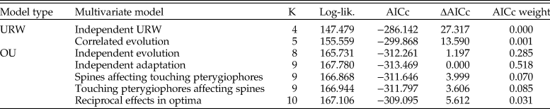
Table 4. Maximum likelihood parameter estimates for the candidate models fit to the multivariate evolutionary sequence of stickleback armor trait evolution. URW, unbiased random walk.

Discussion
Analysis of evolutionary time series in the rock record represents a unique contribution from paleontology to further the development of evolutionary biology. For example, the adaptive landscape has for decades been suggested as a conceptual bridge to bring our understanding of microevolution and macroevolution closer to one another (e.g., Simpson Reference Simpson1944; Arnold et al. Reference Arnold, Pfrender and Jones2001; Hansen Reference Hansen, Svensson and Calsbeek2012). Shifts in the adaptive landscape along branches of a phylogeny using OU processes are commonly explored (e.g., Ingram and Mahler Reference Ingram and Mahler2013; Uyeda and Harmon Reference Uyeda and Harmon2014; Khabbazian et al. Reference Khabbazian, Kriebel, Rohe and Ané2016), but whether detected shifts in optima represent sudden and major changes of the adaptive landscape or whether they instead reflect cumulative changes in the position of adaptive peaks across time is poorly known (e.g., Uyeda and Harmon Reference Uyeda and Harmon2014). Inferring the dynamics of the adaptive landscape through analysis of evolutionary time series may shed light on this and other questions regarding the dynamic nature of the adaptive landscape at different temporal scales. This potential is exemplified by the reanalysis of size evolution in the radiolarian lineage Eucyrtidium calvertense. The best-fit model for the E. calvertense data suggests that size evolution in the lineage was affected by a major and sudden change in the adaptive landscape, while a model where the adaptive landscape changed more gradually had a poorer, but still similar, fit.
Multivariate models allow tests of a range of different hypotheses that are difficult to assess by relying on univariate models only. Two traits that appear to evolve together (i.e., show correlated evolution) over time may, for example, be influenced by the same selective agent (e.g., temperature). Another possibility is that only one of the traits is directly affected by the selective agent and that changes in this trait lead to changes in the optimal value of the second trait, resulting in a somewhat lagged evolutionary response in the second trait relative to the first trait. Investigating competing explanations for multivariate trait dynamics requires a multivariate approach. The reanalysis of the stickleback data (Bell et al. Reference Bell, Travis and Blouw2006; Hunt et al. Reference Hunt, Bell and Travis2008) examined various hypotheses regarding evolution and adaptation in two armor traits. The results support independent evolution of each armor trait toward separate optima on the adaptive landscape, but a substantial portion of the stochastic changes in the two traits were correlated. The field of quantitative genetics has convincingly demonstrated how genetic correlations may affect phenotypic evolution (Lande Reference Lande1979; Lande and Arnold Reference Lande and Arnold1983; Walsh and Blows Reference Walsh and Blows2009), and some armor traits in extant threespine stickleback have been found to covary genetically (e.g., Cresko et al. Reference Cresko, Amores, Wilson, Murphy, Currey, Phillips, Bell, Kimmel and Postlethwait2004; Leinonen et al. Reference Leinonen, Cano and Merilä2011), suggesting these traits are likely to have a reduced capacity to evolve completely independently of each other. One possible interpretation of the detected non-independence in part of the evolution of the two armor traits is therefore due to a shared genetic background. An alternative and not mutually exclusive explanation is that these two armor traits have experienced correlated selection.
It is important to note that the interpretation of the various univariate and multivariate trait models in evoTS (and paleoTS) may vary depending on the time interval covered by the data analyzed. For example, the OU process has been used to describe microevolutionary changes in a population close to a fixed peak in the adaptive landscape (Lande Reference Lande1976; Hansen and Martins Reference Hansen and Martins1996), but it is also commonly used to model evolution within and between adaptive zones on among-species comparative data (e.g., Mahler et al. Reference D. L., Ingram, Revell and Losos2013; Moen et al. Reference Moen, Morlon and Wiens2016; Toljagić et al. Reference Toljagić, Voje, Matschiner, Liow and Hansen2018). Fitting OU models to evolutionary time series of modern lineages where the data have a generational resolution allows for the estimation of microevolutionary parameters and the development of a process-based interpretation of the trait dynamics based on the parameters in the OU model (for an example, see Lo Cascio Sætre et al. Reference Lo Cascio Sætre, Coleiro, Austad, Gauci, Sætre, Voje and Eroukhmanoff2017). The fossil record may not always have the necessary resolution for interpreting the model directly in terms of microevolutionary processes, in which case a more phenomenological interpretation of the fitted models may be more appropriate. For example, interpreting the stochastic part of the trait dynamics in an OU model as primarily a result of genetic drift may be more suitable when fitting the model to modern data with high time resolution than when fitting it to data with lower time resolution (Hansen et al. Reference Hansen, Pienaar and Orzack2008). However, there is no strict boundary between when a process-based and when a more phenomenological interpretation is most suitable. In their analysis of the same fossil stickleback lineage analyzed in this study, Hunt et al. (Reference Hunt, Bell and Travis2008) demonstrated that microevolutionary parameters can be meaningfully estimated when fitting the OU model to data from the fossil record. Therefore, the best way to interpret the model parameters should be assessed on a case-by-case basis.
The number of models and software available for conducting phylogenetic comparative analyses have steadily increased for more than 30 years, giving ample opportunities for exploring a large range of hypotheses of trait dynamics on macroevolutionary timescales (e.g., see Pennell and Harmon Reference Pennell and Harmon2013). Analysis of evolutionary time series has not experienced a similar momentum, likely due to the smaller number of available evolutionary time series relative to phylogenetic comparative data. The R package paleoTS has for a long time been the most popular software for fitting models to evolutionary time series. The implemented univariate and multivariate models in evoTS extend the model options available in paleoTS. However, evoTS is not the only software that allows fitting models to evolutionary time series. layeranalyzer (Reitan and Liow Reference Reitan and Liow2019) is a tool that can be used to explore correlations and causal relationships among variables in time series and can fit most of the models implemented in evoTS. mvmorph (Clavel et al. Reference Clavel, Escarguel and Merceron2015) is mainly targeted toward analysis of multivariate phylogenetic comparative data, but several of the implemented models can also be fit to time series. The main advantage of evoTS is that it works as an extension of the much-used paleoTS framework and is therefore specifically tailored toward analysis of evolutionary time series. The combined suite of univariate and multivariate models in paleoTS and evoTS is also not found in any alternative software.
Connecting known microevolutionary processes to macroevolutionary patterns remain a central challenge in biology (e.g., Jablonski Reference Jablonski2000, Reference Jablonski2017; Arnold et al. Reference Arnold, Pfrender and Jones2001; Hansen Reference Hansen, Svensson and Calsbeek2012). While data on generational changes and among-taxa differences are readily available for many organismal groups, information on how lineages evolve in between micro- and macroevolutionary timescales is rare in comparison. Furthermore, how to interpret evolutionary change recorded in the rock record has been debated for decades (e.g., Eldredge and Gould Reference Eldredge, Gould, Schopf and Thomas1972; Charlesworth et al. Reference Charlesworth, Lande and Slatkin1982; Gingerich Reference Gingerich1984, Reference Gingerich2019; Stanley Reference Stanley1985; Bookstein Reference Bookstein1987; Hunt Reference Hunt2007; Voje Reference Voje2016), and the nature of evolutionary change within lineages remains controversial (Lieberman and Eldredge Reference Lieberman and Eldredge2014; Pennell et al. Reference Pennell, Harmon and Uyeda2014a,Reference Pennell, Harmon and Uyedab; Venditti and Pagel Reference Venditti and Pagel2014). Investigating and comparing a larger range of models and hypotheses when analyzing phenotypic change within lineages may contribute to these ongoing discussions.
Acknowledgments
I thank K. Bartoszek, T. F. Hansen, and T. Reitan for discussions and their patience when explaining the nuts and bolts of various models of evolution to me. I owe huge thanks to G. Hunt for being supportive, helpful (including notifying me of an error in my code), and encouraging while I was developing evoTS. V. B. Kinneberg and M. Thaureau tested evoTS and made suggestions that improved the user experience of the R package. J. Crampton, G. Hunt, and an anonymous reviewer provided reviews that improved the work. Thanks also to M. Grabowski, L. H. Liow, and J. Saulsbury for comments on earlier versions of this article. The work was supported by an ERC–2020–STG (grant agreement ID: 948465).
Declaration of Competing Interests
The author declares no competing interests.
Data Availability Statement
The R package evoTS is available for download from the Comprehensive R Archive Network (CRAN). Data and R code are available from the Dryad Digital Repository: https://doi.org/10.5061/dryad.c59zw3rcp.


 Open access