

1. Introduction
Bargaining games have played an important role in models of the evolution of social conventions, particularly with regard to norms around fairness and distributive justice (see Binmore Reference Binmore2005, Reference Binmore2014; Skyrms Reference Skyrms2014; O’Connor Reference O’Connor2019; Alexander and Skyrms Reference Alexander and Skyrms1999; Axtell et al. Reference Axtell, Epstein and Young2000). In particular, they have been used in analyses of the emergence of social contracts and, furthermore, to what extent such contracts or conventions will be efficient or fair toward all agents.
These games represent situations in which agents must decide how to divide a finite resource. Such situations may arise whenever humans jointly produce or discover shareable goods and must allocate who receives what proportion. Each wants to earn as much as possible, but they cannot collectively claim more than the resource’s total value.
These models have generally rested on the assumption that there is a predetermined, finite set of strategy options from which the agents must choose. This fixed set of strategies is an artificial imposition: in nature, any strategy must be invented, for example, through learning or evolution. This idea of agents inventing new strategies has only recently begun to be explored, in certain game theoretic contexts like signaling games (see Young Reference Young1993; Schreiber Reference Schreiber2001; Alexander et al. Reference Alexander, Skyrms and Zabell2012). They have demonstrated that different evolutionary outcomes can arise in such cases, suggesting the importance of applying invention models to other situations.
Invention can serve a particularly important role in understanding how or why a social contract or convention might evolve. We cannot suppose that agents begin with a cooperative strategy in mind. We might imagine agents beginning in a state of conflict or war, in which each agent seeks to claim a resource for herself, from which cooperative strategies may, or may not, evolve.Footnote 1 Or we could imagine agents starting from an entirely neutral position, with no initial strategies at all.
I seek to understand better whether agents can learn or evolve social conventions naturally in a bargaining situation. Of particular interest is the extent to which evolved social conventions will be fair or efficient in their allocation of resources. To this end, it makes sense to relax this assumption that agents must select from a fixed, finite set of strategies. What is needed is a model of the process of the evolution of agents interacting in which strategies must be invented, rather than handed out to agents at the start of the game.
I present a new dynamical model of agents learning in bargaining games in which new strategies must be invented and reinforced. I consider two starting conditions. First, I consider an initial condition in which agents begin in a state of conflict, only able to demand the whole value of the resource or none at all—a hypothetical“state of nature” in which cooperation has not been learned or evolved. Second, I consider a “neutral” initial condition, in which the agents start with no initial strategies at all and all strategies must be invented. Such models should provide a further step toward understanding whether, and how, agents can learn or evolve social conventions naturally.
I use simulations to study the dynamics of the model and to test the extent to which it leads to outcomes that are fair or efficient. On average, the players make demands that peak a little below the fair solution, but with a moderate variation of outcomes on any particular run. The players’ rewards are on average a little lower than their demands, with a similar variability. The strategies are somewhat inefficient, with around 15 percent of the resource being wasted on average. I investigate several modifications of the model by implementing three different forms of forgetting and restricting the set of strategies that can be invented. One form of forgetting increases the average fairness, decreases the variation, and improves the efficiency; a second form widens the variation, with little change to the efficiency; the third increases fairness at the expense of efficiency. I also investigate a method of restricting the possible strategies, which has little overall effect on the fairness and efficiency.
In section 2, I provide some background to the model. I outline some important results in bargaining games and explain some basic models of invention and forgetting in evolutionary contexts. In section 3, I provide a more detailed description and present the results from running the model. In section 4, I propose three methods by which the agent may also forget strategies as well as invent them. In section 5, I modify the model to restrict the strategies that can be invented. In section 6, I adapt the model to a single, finite population, better suited to represent evolutionary dynamics.
2. Background and literature
2.1 Bargaining games and divide-the-dollar
In a bargaining game, two agents compete over a resource. Each demands some fraction. The Nash demand game provides a model of bargaining situations in which two players may each demand any proportion of the resource. If their demands sum to less than the resource’s total value, each receives her demands. If the demands exceed the value of the resource, the players receive a fixed low payoff, often set to zero, representing the failure to come to an agreement.Footnote 2
More precisely, the agents have access to any agreements in some convex feasibility set, $S \subset{\mathbb{R}^2}$
. If agents can agree on some choice within the feasibility set, then they get these corresponding payoffs. Otherwise, their payoffs come from a disagreement point,
$S \subset{\mathbb{R}^2}$
. If agents can agree on some choice within the feasibility set, then they get these corresponding payoffs. Otherwise, their payoffs come from a disagreement point, $d=(d_1, d_2)$
, where
$d=(d_1, d_2)$
, where $d_1$
and
$d_1$
and $d_2$
are the rewards each player receives in this case. Divide-the-dollar is a special case of this game, in which the two agents are identical, with the the same disagreement points and the same utility functions, with utilities proportional to the fraction of the resource earned.
$d_2$
are the rewards each player receives in this case. Divide-the-dollar is a special case of this game, in which the two agents are identical, with the the same disagreement points and the same utility functions, with utilities proportional to the fraction of the resource earned.
Bargaining games have played a pivotal role in studies of distributive justice (Binmore Reference Binmore2005, Reference Binmore2014; Skyrms Reference Skyrms2014; O’Connor Reference O’Connor2019; Alexander and Skyrms Reference Alexander and Skyrms1999; Axtell et al. Reference Axtell, Epstein and Young2000). They are used in explanations of human preferences toward fair outcomes, as well as the processes by which fairness may or may not arise. Intuitively, one might think of a “fair solution” for two identical agents as one in which both agents receive exactly half the reward. (This will suffice as a meaning of the fair solution in the case of divide-the-dollar. However, one might consider other ideas of fairness in more complicated scenarios [for a discussion, see Sen Reference Sen2009].)
Evolutionary models of bargaining have variously led to mostly fair or unfair outcomes, depending on the modeling assumptions used (see Skyrms Reference Skyrms1994; Young Reference Young1993; Axtell et al. Reference Axtell, Epstein and Young2000; for a review, see O’Connor Reference O’Connor2019, 89–110). The fair solution dominates under replicator dynamics with a single, randomly matched population. An entire population demanding half of a good’s value will always successfully coordinate their demands, whereas a population playing any other strategies will sometimes miscoordinate, and part of the resource will be wasted. As such, the fair solution has the largest basin of attraction (Skyrms Reference Skyrms1994, Reference Skyrms2014).
In contrast to the one-population case, if I divide the population into types,Footnote 3 efficient but unfair outcomes can arise. For example, one type of agent may learn always to make high demands when playing the second type, who learns to demand low against the first type. The outcome is efficient because resources are not wasted when the two types play against each other, yet it is unfair.
2.2 Invention and learning
The model will be based on Roth–Erev-type learning and the Hoppe–Pólya model of invention. I study the Roth–Erev model in particular because it provides an especially natural learning dynamic to combine with an invention process. Here I briefly review these methods. First, I introduce the Pólya model. This can be modified by adding invention, leading to the Hoppe–Pólya model, or by adding differential reinforcement. Models with differential reinforcement include Roth–Erev learning and the Schreiber model of evolution for finite populations.
In the unmodified Pólya urn model, I represent objects of interest with balls within an urn, with a finite number of colors, where each color represents a different category of object. Each round, a ball is drawn from the urn and then returned. This process is random, with each ball having equal probability of being drawn. Each time a ball is drawn, a second ball of the same color is also added to the urn. All colors are treated identically, but colors that have been drawn many times will accumulate more balls. As a result, the probability of further reinforcement increases with the proportion of balls of that color. With probability 1, the limiting probabilities of each color will converge, although they could converge to anything.
The Hoppe–Pólya urn model (Hoppe Reference Hoppe1984) can represent “neutral evolution,” in which there is no selection pressure, or situations of the reinforcement learning process, in which there is no distinction worth learning. I modify the Pólya model by adding a process of invention. I add a “mutator” or “invention” ball to the urn. When I draw the mutator, rather than reinforcing, I add a single ball of a new color to the game, representing the invention of a new category. The color is randomly generated from a uniform distribution over an infinite set of available colors. All color choices are reinforced equally.
Roth and Erev (Reference Roth and Erev1995, Reference Roth and Erev1998) use a model of differential reinforcement to account for the behavior of subjects in experiments, but without invention. The probability of choosing an action is proportional to the total accumulated rewards from choosing it in the past. Schreiber (Reference Schreiber2001) includes differential reinforcement in a finite-population urn model, to represent evolution in finite populations with interacting genotypes. Each round, players are selected at random to play a game, with payoffs representing fitness. Strategies are reinforced in proportion to the payoffs from the game.
If we combine Roth–Erev differential reinforcement with a process of invention, such as that used in the Hoppe–Pólya urn, then we have a model capable of invention and reinforcement. Alexander et al. (Reference Alexander, Skyrms and Zabell2012) apply a model of this sort to represent agents inventing and reinforcing new signals in the context of sender–receiver games with reinforcement learning. I will adapt a similar model to the context of bargaining games (see also Skyrms Reference Skyrms2010).
2.3 Forgetting
Some models of learning and evolution also include a process of “forgetting,” by which unsuccessful strategies become rarer or may go extinct. Forgetting may be realistic in many contexts. It can represent the death of members of an evolutionary population or literal forgetting in the case of individuals. I will study versions of my model both with and without forgetting implemented.
Forgetting may lead to more successful learning outcomes in situations where there are suboptimal equilibria. Barrett and Zollman (Reference Barrett and Zollman2009) study three different learning strategies in signaling games, each of which allows the agents to forget. Significantly, they find that learning rules with forgetting outperform their counterparts without forgetting in such games. They do so by allowing agents to forget past successes that would have driven them to suboptimal equilibria.
Schreiber (Reference Schreiber2001) uses the Pólya urn to model finite populations of different phenotypes (colors). In addition to reinforcement, all balls have a finite probability of being removed from the urn altogether each turn. As a result, phenotypes that are not reinforced will eventually become extinct.
Roth and Erev (Reference Roth and Erev1995) introduce “forgetting” by applying a discount factor that reduces the weights of every strategy, each turn, in an urn-type model. Each weight is multiplied by a factor $(1-x)$
for some
$(1-x)$
for some $x \in (0,1)$
. As a strategy is reinforced more, it will be discounted more, in proportion to its weight. In effect, this caps the maximum possible weight of each strategy at some value, above which it will not grow further.
$x \in (0,1)$
. As a strategy is reinforced more, it will be discounted more, in proportion to its weight. In effect, this caps the maximum possible weight of each strategy at some value, above which it will not grow further.
Alexander et al. (Reference Alexander, Skyrms and Zabell2012) develop models of sender–receiver games in which two different forms of forgetting are implemented. In the first, with some specified probability each round, we pick an urn at random, with an equal probability for each urn, and remove a colored ball at random, with equal probability for each color, from that urn. In the second, with some specified probability each round, we pick an urn at random, then pick a color represented in that urn at random, with an equal probability for each urn, with an equal probability for each color, and remove a ball of that specific color.
3. Basic invention model without forgetting
I study a dynamical model of learning, reinforcement with invention for the the divide-the-dollar game. I use a method of invention based on the Hoppe–Pólya urn, with Roth–Erev-type differential reinforcement. There are two identical agents, players 1 and 2, who must share a resource.Footnote 4 Both have the same utility functions, with utilities proportional to the quantity of the resource that they win. Each player has a list of strategies, including a mutator, with corresponding weights. They reinforce the weights according to the rewards that they receive each turn.
More formally, I assign both agents the same utility function, $u(r)=r$
, where r is the quantity of the resource that they win, with the total value of the resource set equal to 1. Each turn, t, each player,
$u(r)=r$
, where r is the quantity of the resource that they win, with the total value of the resource set equal to 1. Each turn, t, each player, $p \in \{1,2\}$
, has an ordered list of strategies,
$p \in \{1,2\}$
, has an ordered list of strategies, $S^{p,t}=(M^p, s^p_1, \ldots s^p_n)$
, with corresponding weights,
$S^{p,t}=(M^p, s^p_1, \ldots s^p_n)$
, with corresponding weights, $W^{p,t}=(w^{p}_M, w^{p,t}_1,\ldots w^{p,t}_n)$
, where M is the mutator strategy;
$W^{p,t}=(w^{p}_M, w^{p,t}_1,\ldots w^{p,t}_n)$
, where M is the mutator strategy; $s^p_j \in [0,1]$
refers to player p’s jth strategy of demanding some fraction,
$s^p_j \in [0,1]$
refers to player p’s jth strategy of demanding some fraction, $s^p_j$
, of the total resource; and
$s^p_j$
, of the total resource; and $w^{p,t}_j$
is the associated weight at turn t.
$w^{p,t}_j$
is the associated weight at turn t.
Each turn, each player draws a strategy, with probability proportional to its weight:
 $${P^t}(s_j^p) = {{w_j^{p,t}} \over {w_M^p + \sum\limits_{i = 1}^n {w_i^{p,t}} }}.$$
If the sum of both players’ demands comes to less than or equal to 1, then the players reinforce the strategy they just played by the amount that they demanded. I will refer to this as a “successful reinforcement.” If the sum of the demands exceeds 1, then neither player reinforces her strategy. Thus, if strategy $s^p_j$
, with weight
$s^p_j$
, with weight $w^{p,t}_j$
, is successfully reinforced at turn t, then at turn
$w^{p,t}_j$
, is successfully reinforced at turn t, then at turn $t+1$
, we have
$t+1$
, we have $w^{p,t+1}_j = w^{p,t}_j + s^p_j$
; if it is not successfully reinforced, then the weights remain unchanged,
$w^{p,t+1}_j = w^{p,t}_j + s^p_j$
; if it is not successfully reinforced, then the weights remain unchanged, $w^{p,t+1}_j = w^{p,t}_j$
.
$w^{p,t+1}_j = w^{p,t}_j$
.
For example, suppose that at turn t, player 1 chooses strategy $s^1_a = 0.3$
with weight
$s^1_a = 0.3$
with weight $w^{1,t}_a = 1.0$
and player 2 chooses strategy
$w^{1,t}_a = 1.0$
and player 2 chooses strategy $s^2_b = 0.5$
with weight
$s^2_b = 0.5$
with weight $w^{2,t}_b = 1.5$
. Now, these demands sum to
$w^{2,t}_b = 1.5$
. Now, these demands sum to $0.8 \lt 1.0$
, so both players successfully reinforce: the new weights of these strategies will be
$0.8 \lt 1.0$
, so both players successfully reinforce: the new weights of these strategies will be $w^{1,t+1}_a = 1.3$
and
$w^{1,t+1}_a = 1.3$
and $w^{2,t+1}_b = 2.0$
, respectively. Alternatively, suppose that at turn t, player 1 chooses strategy
$w^{2,t+1}_b = 2.0$
, respectively. Alternatively, suppose that at turn t, player 1 chooses strategy $s^1_c = 0.7$
with weight
$s^1_c = 0.7$
with weight $w^{1,t}_c = 1.0$
and player 2 chooses strategy
$w^{1,t}_c = 1.0$
and player 2 chooses strategy $s^2_d = 0.4$
with weight
$s^2_d = 0.4$
with weight $w^{2,t}_d = 1.4$
. Now, these demands sum to
$w^{2,t}_d = 1.4$
. Now, these demands sum to $1.1 \gt 1.0$
, so the players earn rewards of 0, and the weights are unchanged:
$1.1 \gt 1.0$
, so the players earn rewards of 0, and the weights are unchanged: $w^{1,t+1}_c = 1.0$
and
$w^{1,t+1}_c = 1.0$
and $w^{2,t+1}_d = 1.4$
, respectively.
$w^{2,t+1}_d = 1.4$
, respectively.
Each turn, each player may draw the mutator, with probability
 $${P^t}({M^p}) = {{w_M^p} \over {w_M^p + \sum\limits_{i = 1}^n {w_i^{p,t}} }}.$$
Then the corresponding player “invents” a new strategy by drawing from a uniform distribution over all possible demands in the interval $[0,1]$
.Footnote 5 Upon inventing a new strategy, the player adds this to her ordered list of playable strategies and plays this strategy, reinforcing the weight accordingly. The other player picks her demand and plays the turn as usual. Thus, if, at turn t, player p has the set of n strategies,
$[0,1]$
.Footnote 5 Upon inventing a new strategy, the player adds this to her ordered list of playable strategies and plays this strategy, reinforcing the weight accordingly. The other player picks her demand and plays the turn as usual. Thus, if, at turn t, player p has the set of n strategies, $S_{p,t}=(M^p, s^p_1, \ldots s^p_n)$
, with weights
$S_{p,t}=(M^p, s^p_1, \ldots s^p_n)$
, with weights $W^{p,t}=(w^{p}_M, w^{p,t}_1,\ldots s^{p,t}_n)$
, and draws the mutator strategy, selecting strategy
$W^{p,t}=(w^{p}_M, w^{p,t}_1,\ldots s^{p,t}_n)$
, and draws the mutator strategy, selecting strategy $s^p_{n+1}$
, then the new set of strategies will be
$s^p_{n+1}$
, then the new set of strategies will be $S_{p,t+1}=(M^p, s^p_1, \ldots s^p_n, s^p_{n+1},)$
, with weights
$S_{p,t+1}=(M^p, s^p_1, \ldots s^p_n, s^p_{n+1},)$
, with weights $W^{p,t}=(w^{p}_M, w^{p,t}_1,\ldots w^{p,t}_{n+1})$
.
$W^{p,t}=(w^{p}_M, w^{p,t}_1,\ldots w^{p,t}_{n+1})$
.
The agents begin with a limited initial collection of strategies: $S^{p,0}= (M, 0, 1)$
,
$S^{p,0}= (M, 0, 1)$
, $W^{p,0} =(1,1,1)$
; that is, the players may demand everything, relinquish everything, or invent a new strategy. The dynamics will allow us to study agents learning to negotiate by inventing compromise strategies in which they demand some fraction of the resource.Footnote 6
$W^{p,0} =(1,1,1)$
; that is, the players may demand everything, relinquish everything, or invent a new strategy. The dynamics will allow us to study agents learning to negotiate by inventing compromise strategies in which they demand some fraction of the resource.Footnote 6
The mutator strategy is not reinforced, so the probability with which the mutator is selected will decrease as the number of balls in the urn increases. Thus, in this basic model, as new strategies are invented, or existing strategies are reinforced, the probability that the mutator is drawn will fall. At the beginning, the rate of invention will be high, but this rate will gradually drop off.
From this small number of strategies as a starting point, one can see how the process evolves. As with the number of balls in the Hoppe–Pólya urn model, the limiting number of different strategies for each player will be infinite; one can further show that the number of times each player will play each strategy diverges. I prove these claims in Appendixes B and C.
Let us walk through the first few turns of an imagined scenario as an example. Player 1 and player 2 each starts with just the three basic strategies. Suppose that on turn 1, player 1 draws demand 1 and player 2 draws demand 1. The sum of the demands exceeds 1, so neither player reinforces. Now, suppose that for turn 2, player 1 draws demand 0 and player 2 draws demand 1. The sum of these demands does not exceed 1, so both players reinforce: player 2 reinforces that strategy by her reward of 1, $W^{p=2,t=2} = (1,1,2)$
, and is more likely to play it again. However, player 1’s reward is zero, so her weights remain unchanged. In turn 3, let us suppose that player 1 draws the mutator ball and selects a new strategy, demand 0.4. Player 2 plays demand 0. These sum to less than 1, so again, the players reinforce. Now player 1’s strategies and weights are
$W^{p=2,t=2} = (1,1,2)$
, and is more likely to play it again. However, player 1’s reward is zero, so her weights remain unchanged. In turn 3, let us suppose that player 1 draws the mutator ball and selects a new strategy, demand 0.4. Player 2 plays demand 0. These sum to less than 1, so again, the players reinforce. Now player 1’s strategies and weights are $S^{p=1,t=3}= (M, 0, 1, 0.4)$
,
$S^{p=1,t=3}= (M, 0, 1, 0.4)$
, $W^{p=1,t=3}= (1,1,1,0.4)$
; player 1’s strategies and weights are
$W^{p=1,t=3}= (1,1,1,0.4)$
; player 1’s strategies and weights are $S^{p=2,t=3}= (M, 0, 1)$
,
$S^{p=2,t=3}= (M, 0, 1)$
, $W^{p=2,t=3}= (1,1,2)$
.
$W^{p=2,t=3}= (1,1,2)$
.
3.1 Basic model: Results
I observe the results from ten thousand runs of the simulation. Each run covers one hundred thousand turns, appropriate for an investigation of the “intermediate dynamics” of this model. The histograms in Figure 1 show certain key results. Shown are histograms of the average rewards and demands in each run, averaged for both players and averaged over all one hundred thousand turns. These histograms show how much players were demanding or receiving in reward, on average, for each of the ten thousand simulation runs. Likewise, I show histograms, for each run, of the mean demand differences and reward differences between the two players, averaged over all one hundred thousand turns. These histograms indicate how much player 1 was demanding or receiving more or less than player 2, on average, for each of the ten thousand simulation runs.
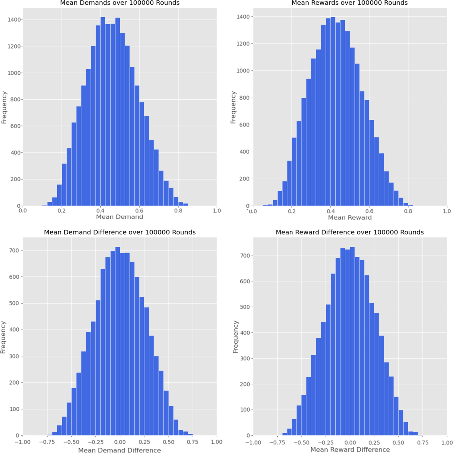
Figure 1. Results from ten thousand runs of the simulation. (top) Frequency of runs against mean demands and rewards over one hundred thousand turns. (bottom) Frequency of runs against mean demand and reward differences, between players 1 and 2, over one hundred thousand turns.
The demand and reward histograms peak a little below the fair solution, indicating that in most runs, players demand and receive rewards a little below one-half, on average, across all one hundred thousand turns. However, in many particular runs, players may make demands and receive rewards some way above or below this, on average, across all one hundred thousand turns. The histograms of reward and demand differences give some indication of the unfairness between the two players: these histograms peak around 0, indicating that in many runs, the demands and rewards are close to equal, averaged over one hundred thousand turns. However, in many runs, one player or the other systemically demands or receives more than the other, across the one hundred thousand turns.
Table 1 summarizes further results. Mean outcomes are calculated for each player by averaging over each turn; averages are then taken over all the simulation runs. Player mean demands are found to fall within the interval $[0.4,0.6]$
49 percent of the time, and player mean rewards fall within the interval
$[0.4,0.6]$
49 percent of the time, and player mean rewards fall within the interval $[0.4,0.6]$
46 percent of the time.
$[0.4,0.6]$
46 percent of the time.
Table 1. Results from ten thousand runs of the simulation
| Mean | Standard deviation | |
|---|---|---|
| Demands | 0.46 | 0.13 |
| Rewards | 0.42 | 0.13 |
| Signed demand difference | 0.00 | 0.26 |
| Signed reward difference | 0.00 | 0.25 |
| Absolute demand difference | 0.21 | 0.14 |
| Absolute reward difference | 0.20 | 0.15 |
Note. Each run covers one hundred thousand turns. Mean demands and rewards are shown for each player, as are the signed and absolute differences in the demands and rewards. Outcomes are averaged for each player, over one hundred thousand turns for each run; the means and standard deviations are then taken for the distributions of both players over all ten thousand runs.
Means and standard deviations of the player mean demands are calculated as follows. First, I find the average demands for players 1 and 2 each turn, and then over all one hundred thousand turns, for each individual run. Then, I take the mean and standard deviation of the distribution for both players over all ten thousand runs. I calculate the means and standard deviations for the player mean rewards, signed differences, and absolute differences analogously. I define the signed and absolute differences in player demands as follows. Let player 1’s demand in some turn be $D_1$
, and let players 2’s demand be
$D_1$
, and let players 2’s demand be $D_2$
. Then, the signed difference is given by
$D_2$
. Then, the signed difference is given by $D_1 - D_2$
. The absolute difference is defined by
$D_1 - D_2$
. The absolute difference is defined by $|D_1 - D_2|$
. Once again, I take the average over all one hundred thousand turns for each individual run and then calculate the means and standard deviations of the distributions of the signed and absolute differences over all ten thousand runs.
$|D_1 - D_2|$
. Once again, I take the average over all one hundred thousand turns for each individual run and then calculate the means and standard deviations of the distributions of the signed and absolute differences over all ten thousand runs.
The means give an indication of average outcomes, but the standard deviations inform us how much an individual run might typically deviate from that average. For example, a mean demand close to 0.5 and a very narrow standard deviation would suggest that the players typically make demands close to the fair solution. The signed difference between the two players’ demands and rewards should always be close to zero, providing a check that the two players are treated identically. The standard deviation of the signed difference between the two players gives an indication of how unequal the two players’ demands and rewards are on average. The absolute value of the difference between the two players’ demands and rewards gives us a second indication of how unequal the two players’ demands and rewards are on average, given that the signed difference should be zero on average.
3.2 Basic model: Analysis
Fair outcomes are favored strongly, but by no means overwhelmingly. Mean demands peak a little below the fair solution of 0.5; however, in a typical run, the players may vary some way from this. Mean rewards are a little lower than mean demands. Many runs result in outcomes quite far from the fair solution. Furthermore, the players are somewhat, but not completely, efficient. Even after one hundred thousand turns, around ${1}/{15}$
of the resource is wasted on average each turn. Sometimes the players overshoot, making collective demands that sum to greater than 1; at other times they undershoot, with demands that sum well below 1. The mean rewards have a lower peak than the demands due to overshooting in particular.
${1}/{15}$
of the resource is wasted on average each turn. Sometimes the players overshoot, making collective demands that sum to greater than 1; at other times they undershoot, with demands that sum well below 1. The mean rewards have a lower peak than the demands due to overshooting in particular.
The distributions of the differences between the rewards and demands reveal that the two players are symmetric, as expected. The standard deviation and mean signed difference suggest that in any particular run of the simulation, the players are close together in their demands, but not wholly balanced in a typical run. Outcomes are somewhat, but not wholly, fair.
It seems that certain factors may be favoring fair outcomes but are not sufficiently strong to guarantee that a wholly fair outcome will result. In the early turns, players generally start by opting for 0 or 1 but soon invent and deploy new strategies. The rate of mutations is high, and strategies are not yet highly reinforced. After a large number of turns have taken place, both players generally settle on either a single strategy or a cluster of similar strategies (in which the player demands a similar proportion of the resource each turn). The sum of the two players’ typical demands is usually a little below 1.
Why does a degree of inequality persist under these dynamics? Luck plays an important role, especially early on, when strategies have not been highly reinforced and when the rate of invention is still high. Suppose that player 1 has a few lucky successes with a high-demand strategy early, let us say, demand x; then this strategy may be highly reinforced. In response to this strategy, player 2 will only positively reinforce strategies that demand $1-x$
or less. Over time, the rate of invention decreases, and both players settle into this unfair outcome.
$1-x$
or less. Over time, the rate of invention decreases, and both players settle into this unfair outcome.
However, the resultant rewards for both players may be low. Player 2’s low-reward strategies will be reinforced, but by a small amount. As a result, the probability of choosing the mutator may remain relatively higher than it would otherwise, so player 2 may also continue to experiment with other strategies for longer. If player 1’s demands are very high, there is a high chance that the players will overshoot in their demands, especially when player 2 is experimenting, resulting in both players earning no reward. As a result, player 1’s very-high-demand strategy may not continue to receive further high rewards, and the player may eventually settle on a lower demand strategy.
The persistence of unfairness is unsurprising. Given that the model involves two interacting agents, it is possible (in principle) for the two agents to coordinate on an unfair equilibrium that is still efficient. For example, player 1 might demand $0.75$
almost always, and player 2 might demand
$0.75$
almost always, and player 2 might demand $0.25$
, resulting in an efficient outcome. This could be compared to the two-type dynamics I explained in section 2.1. Of course, in practice, given that the strategies are drawn from a random, uniform distribution, the players will almost never perfectly coordinate after a finite number of terms. One should expect some inefficiency to persist. However, with time, agents might adopt strategies that reduce this inefficiency.
$0.25$
, resulting in an efficient outcome. This could be compared to the two-type dynamics I explained in section 2.1. Of course, in practice, given that the strategies are drawn from a random, uniform distribution, the players will almost never perfectly coordinate after a finite number of terms. One should expect some inefficiency to persist. However, with time, agents might adopt strategies that reduce this inefficiency.
The combination of these factors leads to average demands peaking a little below the fair division, but with a wide spread of possibilities. Likewise, the two players’ rewards after one hundred thousand turns sum only to around 0.85 on average, revealing a moderate degree of inefficiency. A significant proportion of the resource is wasted, granted to neither player.
4. Invention model with forgetting
In section 2.3, I argued that some models of evolution or learning should perhaps include the possibility of strategies being forgotten or even going extinct. Furthermore, there is some evidence that forgetting can promote learning in games that have suboptimal equilibria (Barrett and Zollman Reference Barrett and Zollman2009). Let us adapt the three forms of forgetting suggested by Alexander et al. (Reference Alexander, Skyrms and Zabell2012) and Roth and Erev (Reference Roth and Erev1995). Using the analogy of balls in urns, first, we might imagine that with some finite probability each turn, nature picks a ball at random of any color and removes it from the urn. Second, we might imagine that with some finite probability each turn, nature picks a color at random and removes a ball of that color. That is, the natural process might reduce the weight of each strategy with equal probability or in proportion to the weight assigned to that strategy. Finally, we might imagine a form of forgetting in which nature simply discounts the weight of every strategy every turn by some amount proportional to its weight.
Each method of forgetting takes place, for each player, at the start of each turn. For the first two, I have some assigned probability of forgetting $p_f$
, set equal for both players. A second parameter,
$p_f$
, set equal for both players. A second parameter, $r_f$
, determines the quantity by which the forgetting reduces a chosen strategy’s weight. I label the two types of forgetting as follows:
$r_f$
, determines the quantity by which the forgetting reduces a chosen strategy’s weight. I label the two types of forgetting as follows:
Forgetting A. One of the player’s strategies is chosen at random, with probability proportional to its weight. The weight assigned to this strategy is reduced by $r_f$
. If the strategy’s weight is already less than
$r_f$
. If the strategy’s weight is already less than $r_f$
, then the strategy’s weight is set to 0.
$r_f$
, then the strategy’s weight is set to 0.
Forgetting B. One of the player’s strategies is chosen at random, with equal probability assigned to each strategy. The weight assigned to this strategy is reduced by $r_f$
. If the strategy’s weight is already less than
$r_f$
. If the strategy’s weight is already less than $r_f$
, then the strategy’s weight is set to 0.
$r_f$
, then the strategy’s weight is set to 0.
The third type of forgetting depends on a single parameter, $d_f$
: Roth–Erev discounting. The weight of each strategy (except for the mutator) for each agent is multiplied by the discount factor,
$d_f$
: Roth–Erev discounting. The weight of each strategy (except for the mutator) for each agent is multiplied by the discount factor, $(1-d_f)$
, each turn.
$(1-d_f)$
, each turn.
4.1 Forgetting A: Results
I observe the results from ten thousand runs of the simulation of this model, each over one hundred thousand turns, with forgetting method A implemented and $p_f = 0.3$
and
$p_f = 0.3$
and $r_f = 1$
for both players. In Figure 2, I show the mean demands and rewards for each player, averaged over all turns, as well as the differences between the average demands and the average rewards for the two players. I summarize the results, averaged for the two identical players, in Table 2. Player mean demands fall within the interval
$r_f = 1$
for both players. In Figure 2, I show the mean demands and rewards for each player, averaged over all turns, as well as the differences between the average demands and the average rewards for the two players. I summarize the results, averaged for the two identical players, in Table 2. Player mean demands fall within the interval $[0.4,0.6]$
66 percent of the time, and player mean rewards also fall within this interval 66 percent of the time significantly higher than in the no-forgetting case. With forgetting method A implemented, many more runs lie close to the fair solution, and the results are more efficient.
$[0.4,0.6]$
66 percent of the time, and player mean rewards also fall within this interval 66 percent of the time significantly higher than in the no-forgetting case. With forgetting method A implemented, many more runs lie close to the fair solution, and the results are more efficient.
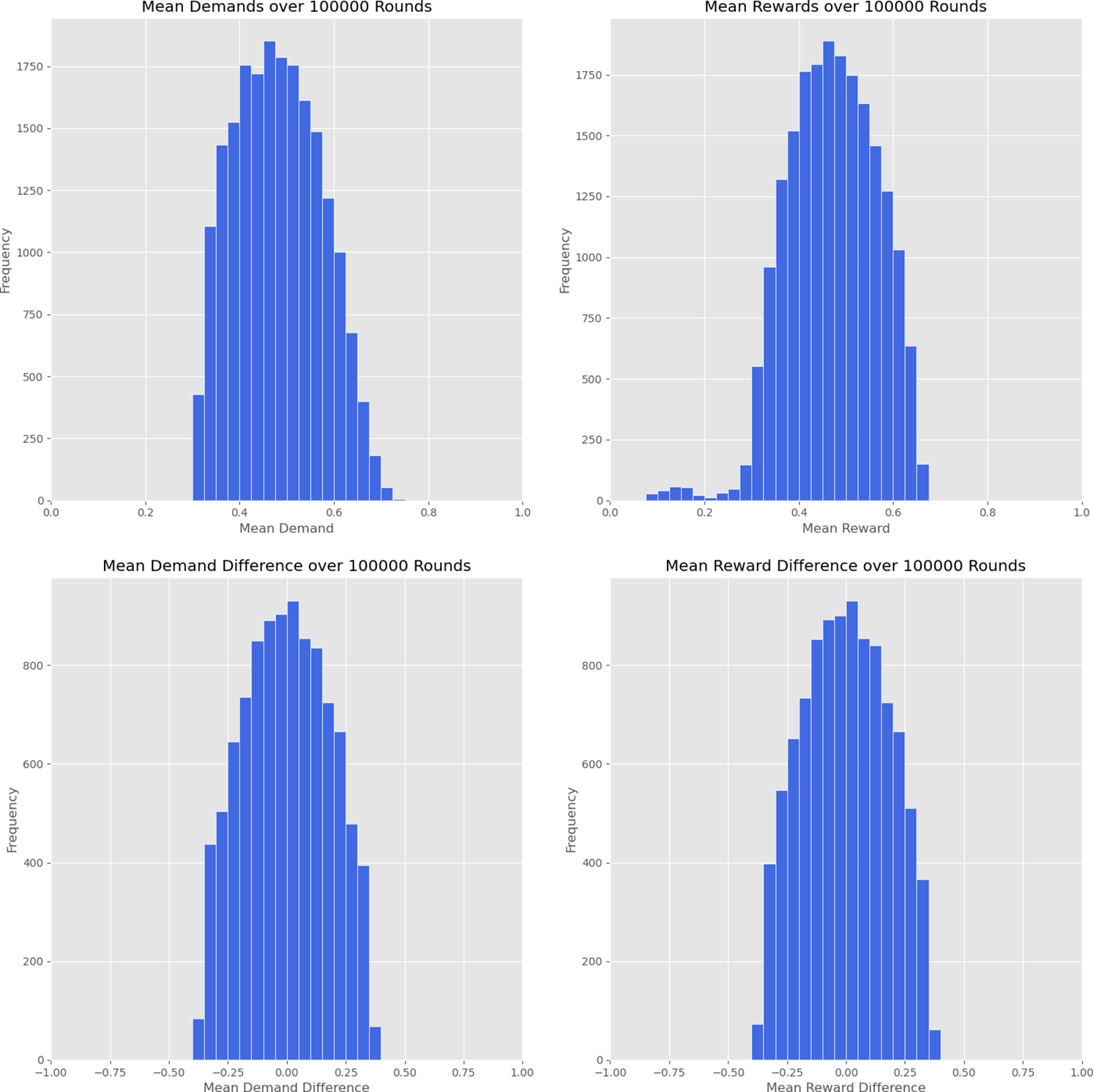
Figure 2. Results from running ten thousand runs of the simulation, for one hundred thousand turns each, with forgetting method A, $p_f = 0.3$
,
$p_f = 0.3$
, $r_f = 1$
, for each player. (top) Frequency of runs against mean demands and rewards over one hundred thousand turns. (bottom) Frequency of runs against mean demand and reward differences, between players 1 and 2, over one hundred thousand turns.
$r_f = 1$
, for each player. (top) Frequency of runs against mean demands and rewards over one hundred thousand turns. (bottom) Frequency of runs against mean demand and reward differences, between players 1 and 2, over one hundred thousand turns.
Table 2. Results from running ten thousand runs of the simulation, for one hundred thousand turns each, with forgetting method A
| Mean | Standard deviation | |
|---|---|---|
| Demands | 0.48 | 0.09 |
| Rewards | 0.47 | 0.09 |
| Signed demand difference | 0.00 | 0.18 |
| Signed reward difference | 0.00 | 0.18 |
| Absolute demand difference | 0.15 | 0.09 |
| Absolute reward difference | 0.15 | 0.10 |
Note. Mean demands and rewards are shown for each player, as are the signed and absolute differences in the demands and rewards. Average outcomes are calculated for each player, over one hundred thousand turns for each run; the means and standard deviations are then taken for the distributions of both players over all ten thousand runs.
4.2 Forgetting A: Analysis
Interestingly, introducing forgetting A changes the distribution shape significantly as compared to the case in which no forgetting takes place. Mean demands for each player are a little higher than in the case of no forgetting, but with a clearly right-skewed distribution. Mean rewards average significantly higher than the no-forgetting case, but this distribution is left-skewed, with a long tail. Large differences between the two players’ rewards or demands are significantly more rare.
Forgetting method A provides a more ruthless evolutionary environment, red in tooth and claw, for successful strategies especially. Strategies that are reinforced are also more likely to experience some forgetting, in proportion to their weight. As a result, only strategies that can be reinforced faster than the rate at which they are forgotten will continue to survive and flourish. Low-demand strategies are particularly punished: they can rarely reinforce fast enough to overcome the rate of forgetting. High-demand strategies are also punished, but they may survive more often. These strategies can lead to a high enough rate of reinforcement, as long as the other player does not also reinforce high-demand strategies. This results in the skewed shape of the distributions seen.
For example, suppose that player 2 has highly reinforced the strategy demand 0.75. Then, player 1 will be most rewarded with a strategy of demanding something close to 0.25; let us suppose that she begins to reinforce the strategy demand 0.2, and this becomes her highest-weight strategy. However, under forgetting method A, player 1 is also most likely to forget this strategy: if it is her only strategy, then she has a $p_f = 0.3$
chance to forget this strategy each turn, reducing it by
$p_f = 0.3$
chance to forget this strategy each turn, reducing it by $r_f = 1$
. In the limit that this were player 1’s only strategy, it would have an expected net decrease in weight of
$r_f = 1$
. In the limit that this were player 1’s only strategy, it would have an expected net decrease in weight of $0.1$
each turn, so the strategy would in fact be slowly forgotten. Nor should player 2 expect to benefit from this strategy in the long run: if player 2 plays demand 0.75 and player 1 demands greater than 0.3, then the players will overshoot, and neither will receive any reward.
$0.1$
each turn, so the strategy would in fact be slowly forgotten. Nor should player 2 expect to benefit from this strategy in the long run: if player 2 plays demand 0.75 and player 1 demands greater than 0.3, then the players will overshoot, and neither will receive any reward.
In general, demands of less than $p_f \times r_f$
or greater than
$p_f \times r_f$
or greater than $1-p_f \times r_f$
cannot become dominant in the long run, as they will be forgotten faster than they are reinforced. We see this effect in play in the shape of the distributions: average demands are above 0.3 in all runs and below 0.7 in nearly all runs for both players.Footnote 7
$1-p_f \times r_f$
cannot become dominant in the long run, as they will be forgotten faster than they are reinforced. We see this effect in play in the shape of the distributions: average demands are above 0.3 in all runs and below 0.7 in nearly all runs for both players.Footnote 7
Players are more likely to continue experimenting rather than settling into a low-demand strategy; as a result, the rewards for players who keep making high demands are also lower due to the possibility of overshooting. As a consequence, it is more likely that players will settle close to the fair distribution. The low-reward tail (seen in the mean reward, top right, plot of Figure 2, roughly those cases for which the mean reward $\lesssim 0.3$
) represents cases in which the players still have not settled on a single or close cluster of highly reinforced strategies, even after one hundred thousand turns. However, they do not represent cases in which the players settle on very uneven outcomes: these almost never happen (as seen in the lower two plots of Figure 2). Rather, in such cases, both players are still “experimenting” with a wide variety of strategies.
$\lesssim 0.3$
) represents cases in which the players still have not settled on a single or close cluster of highly reinforced strategies, even after one hundred thousand turns. However, they do not represent cases in which the players settle on very uneven outcomes: these almost never happen (as seen in the lower two plots of Figure 2). Rather, in such cases, both players are still “experimenting” with a wide variety of strategies.
One can build an intuition for why the low-reward tail persists with a simple example. Suppose that player 1 forgets the demand 1 strategy in the first few turns, before she has invented another strategy. Then, the only strategy available to player 1 is to keep playing demand 0. In response, the strategy of player 2 most likely to get reinforced is demand 1. Once the demand 1 outcome is highly reinforced for player 2, player 2 is likely to keep playing it. However, now, it will be hard for player 1 to successfully reinforce any newly invented strategy: any such strategy will give player 1 a reward of 0 if player 2 keeps playing demand 1. Thus any new strategies of player 1 will rarely be reinforced. However, player 2 will often also receive 0 reward whenever player 1 plays any strategy other than demand 0.
The result is that in a few unlucky cases, a highly inefficient outcome will result in which neither player settles on a successful strategy, leading to the low-reward tails. One can gain more information by studying the results of individual simulation runs. I show the results for the first one thousand turns of one such simulation run in Appendix D.
4.3 Forgetting B: Results
I observe the results from ten thousand runs of the simulation of this model over one hundred thousand turns, with forgetting method B implemented and $p_f = 0.3$
and
$p_f = 0.3$
and $r_f = 1$
for both players. In Figure 3, I show the mean demands and rewards for each player, averaged over all turns, as well as the differences between the average demands and the average rewards for the two players. I summarize the results, averaged for the two identical players, in Table 3. Player mean demands fall within the interval
$r_f = 1$
for both players. In Figure 3, I show the mean demands and rewards for each player, averaged over all turns, as well as the differences between the average demands and the average rewards for the two players. I summarize the results, averaged for the two identical players, in Table 3. Player mean demands fall within the interval $[0.4,0.6]$
42 percent of the time, and player mean rewards also fall within this interval 46 percent of the time. More runs result in outcomes far from the fair solution than with forgetting method A or the no-forgetting case.
$[0.4,0.6]$
42 percent of the time, and player mean rewards also fall within this interval 46 percent of the time. More runs result in outcomes far from the fair solution than with forgetting method A or the no-forgetting case.

Figure 3. Results from running ten thousand runs of the simulation, for one hundred thousand turns each, with forgetting method B. (top) Frequency of runs against mean demands and rewards over one hundred thousand turns. (bottom) Frequency of runs against mean demand and reward differences, between players 1 and 2, over one hundred thousand turns.
Table 3. Results from running ten thousand runs of the simulation, for one hundred thouand turns each, with forgetting method B
| Mean | Standard deviation | |
|---|---|---|
| Demands | 0.46 | 0.15 |
| Rewards | 0.46 | 0.16 |
| Signed demand difference | 0.00 | 0.31 |
| Signed reward difference | 0.00 | 0.31 |
| Absolute demand difference | 0.26 | 0.18 |
| Absolute reward difference | 0.26 | 0.18 |
Note. Mean demands and rewards are shown for each player, as are the signed and absolute differences in the demands and rewards. Average outcomes are calculated for each player, over one hundred thousand turns for each run; the means and standard deviations are then taken for the distributions of both players over all ten thousand runs.
4.4 Forgetting B: Analysis
Introducing forgetting B does not change the distribution shape as much as forgetting method A. In section 4.2, we saw that forgetting method A is particularly likely to punish low-demand strategies because they cannot keep up with the rate of forgetting. By contrast, method B is not so likely to punish low-demand strategies: even if they are highly reinforced, a player is just as likely to forget any other strategy.
Averaging over all the simulations, player average demands with forgetting B are similar to those with forgetting A, and so are the average rewards. However, the distribution is wider: the rewards are often further from the fair distribution. The increase in the standard deviations for the demands and rewards reflects the fact that it will usually take longer for players to settle on a cluster of successful strategies. The result is that typical outcomes are less fair than the no-forgetting case.
4.5 Roth–Erev discounting: Results
I observe the results from ten thousand runs of the simulation of this model over one hundred thousand turns, with forgetting Roth–Erev discounting implemented and the same values of $d_f$
for both players. I consider values of
$d_f$
for both players. I consider values of $d_f$
of 0.00, 0.005, 0.01, 0.05, 0.10, 0.50, and 1.00. In Figure 4, I show the mean demands and rewards for each player for the value of
$d_f$
of 0.00, 0.005, 0.01, 0.05, 0.10, 0.50, and 1.00. In Figure 4, I show the mean demands and rewards for each player for the value of $d_f = 0.01$
, averaged over all turns, as well as the differences between the average demands and the average rewards for the two players. I summarize the results, averaged for the two identical players, in Table 4.
$d_f = 0.01$
, averaged over all turns, as well as the differences between the average demands and the average rewards for the two players. I summarize the results, averaged for the two identical players, in Table 4.

Figure 4. Results from running ten thousand runs of the simulation, for one hundred thousand turns each, with Roth–Erev discounting, $d_f = 0.01$
. (top) Frequency of runs against mean demands and rewards over one hundred thousand turns. (bottom) Frequency of runs against mean demand and reward differences, between players 1 and 2, over one hundred thousand turns.
$d_f = 0.01$
. (top) Frequency of runs against mean demands and rewards over one hundred thousand turns. (bottom) Frequency of runs against mean demand and reward differences, between players 1 and 2, over one hundred thousand turns.
Table 4. Results from running ten thousand runs of the simulation, for one hundred thousand turns each, with Roth–Erev discounting $d_f$
$d_f$
|
||||||
|---|---|---|---|---|---|---|
| 0.00 | 0.005 | 0.01 | 0.05 | 0.10 | 0.50 | |
| Mean demands | 0.46 | 0.47 | 0.47 | 0.48 | 0.49 | 0.49 |
| Mean rewards | 0.46 | 0.45 | 0.43 | 0.23 | 0.19 | 0.18 |
| Mean absolute demand difference | 0.26 | 0.19 | 0.15 | 0.01 | 0.00 | 0.00 |
| Mean absolute reward difference | 0.26 | 0.19 | 0.14 | 0.00 | 0.00 | 0.00 |
Note. Average outcomes are calculated for each player, over one hundred thousand turns for each run; the means and standard deviations are then taken for the distributions of both players over all ten thousand runs.
In general, Roth–Erev discounting leads to results that are significantly fairer, yet less efficient, than the no-forgetting case. Furthermore, there is a trade-off: higher values of $d_f$
result in outcomes that are more fair, but less efficient.
$d_f$
result in outcomes that are more fair, but less efficient.
I also observe the results of adding a small error rate in combination with the Roth–Erev discounting. Each agent has a small probability each turn of selecting strategies with uniform probability, rather than in proportion to their weights. I consider three different error probabilities, 0.01, 0.05, and 0.1, for each of the preceding values of $d_f$
. However, the effects of these error rates are small after one hundred thousand turns, changing the mean demands by less than 1 percent and slightly decreasing the mean rewards, by less than 5 percent.
$d_f$
. However, the effects of these error rates are small after one hundred thousand turns, changing the mean demands by less than 1 percent and slightly decreasing the mean rewards, by less than 5 percent.
4.6 Roth–Erev discounting: Analysis
As Roth and Erev (Reference Roth and Erev1995) noted, this form of discounting will effectively put an upper limit on the total weight that can be assigned to any particular strategy. Suppose that some strategy, i, has weight $w^t_i$
at turn t and earns a maximal reward of
$w^t_i$
at turn t and earns a maximal reward of $r_{\text{max}}$
and an expected reward of
$r_{\text{max}}$
and an expected reward of $r_\mu$
each turn. The strategy weights are discounted by a quantity
$r_\mu$
each turn. The strategy weights are discounted by a quantity $w^t_i \times (1-d_f)$
. Once a strategy is reinforced by sufficiently high weight such that
$w^t_i \times (1-d_f)$
. Once a strategy is reinforced by sufficiently high weight such that $w^t_i \times (1-d_f) = r_{\text{max}}$
, it cannot be reinforced further. Moreover, we should expect the strategy no longer to increase average weight after reaching
$w^t_i \times (1-d_f) = r_{\text{max}}$
, it cannot be reinforced further. Moreover, we should expect the strategy no longer to increase average weight after reaching $w^t_i \times (1-d_f) = r_\mu$
.
$w^t_i \times (1-d_f) = r_\mu$
.
Of course, given that I allow infinitely many possible strategies, this does not prevent the invention of a new strategy arbitrarily close to the strategy that has reached its maximum weight. However, the invention of such a strategy will depend on random draws of the mutator, which may take some time. The result is that the total amount of reinforcement is lower, and so the relative probability of drawing the mutator does not decrease to zero as quickly. The two players will keep inventing new strategies for longer, even after having discovered a highly effective strategy. On one hand, this prolonged experimentation helps the players to find strategies that are more fair on average, rather than being trapped in a highly unfair strategy pair. On the other hand, this also leads to a continued high rate of experimentation, causing a considerable degree of overshooting to take place for longer. This results in lower efficiency when the discounting factor is larger.
When the discounting parameter is very large, highly equal outcomes are ensured, because both players will continue to experiment with many strategies. The result is very low efficiency; however, even with very small discounting parameter values, I attain more equal outcomes than the no-forgetting case, with only a small loss in efficiency. In such cases, the increase in fairness arises from the increased experimentation, allowing players to escape being trapped in unfair strategy pairs.
5. Invention with a restricted number of strategies
In many situations, when deciding how to divide a resource, there may be a limited number of possible, or most natural, ways to do so. For example, physical currency has a smallest possible unit. When playing divide-the-dollar with actual currency, it is natural that both players will claim an integer number of cents. When deciding how to divide a presliced pizza, each person might tend to claim an integer number of slices. There is empirical evidence that economic contracts tend to split goods according to simple fractions and that these are resilient under changing circumstances. For example, this has been observed in the records of sharecropping data over long time periods (Young and Burke Reference Young and Burke2001; Allen and Lueck Reference Allen and Lueck2009).
The model can be modified by restricting the set of strategies that may be invented. Previously, once the mutator is drawn, the player draws randomly from a uniform distribution over the interval $[0,1]$
. I will investigate a case for which the strategy is chosen from the set
$[0,1]$
. I will investigate a case for which the strategy is chosen from the set $\{{x}/{20} : x \in \mathcal{N}, 0\leq x \leq 20 \}$
. As I explain in section 3, I allow the same strategy to be “invented” anew multiple times. Multiple copies of the same strategies are reinforced separately. I will refer to this process as restricted invention.
$\{{x}/{20} : x \in \mathcal{N}, 0\leq x \leq 20 \}$
. As I explain in section 3, I allow the same strategy to be “invented” anew multiple times. Multiple copies of the same strategies are reinforced separately. I will refer to this process as restricted invention.
5.1 Restricted invention: Results
I observe the results from ten thousand runs of the simulation of this model over one hundred thousand turns, with restricted invention. I show the results with no forgetting in Figure 5. I summarize the findings with all types of forgetting in Table 5, with parameters $p_f = 0.3$
,
$p_f = 0.3$
, $r_f = 1$
, and
$r_f = 1$
, and $d_f = 0.01$
.
$d_f = 0.01$
.

Figure 5. Results from running simulation for one hundred thousand turns. No forgetting is implemented, and invention is restricted to twenty strategies. (top) Frequency of runs against mean demands and rewards over one hundred thousand turns. (bottom) Frequency of runs against mean demand and reward differences, between players 1 and 2, over one hundred thousand turns. The shape of the peaks is discussed in section 5.2.
Table 5. Results from running ten thousand runs of the simulation, for one hundred thousand turns each with two methods of forgetting and with no forgetting and possible strategies restricted to the set $\{{x}/{20} : x \in \mathcal{N}, 0\leq x \leq 20 \}$
| Mean | Standard deviation | |
|---|---|---|
| No forgetting | ||
| Demands | 0.47 | 0.14 |
| Rewards | 0.44 | 0.14 |
| Signed demand difference | 0.00 | 0.27 |
| Signed reward difference | 0.00 | 0.26 |
| Absolute demand difference | 0.22 | 0.16 |
| Absolute reward difference | 0.22 | 0.15 |
| Forgetting A | ||
| Demands | 0.49 | 0.10 |
| Rewards | 0.48 | 0.10 |
| Signed demand difference | 0.00 | 0.20 |
| Signed reward difference | 0.00 | 0.19 |
| Absolute demand difference | 0.16 | 0.10 |
| Absolute reward difference | 0.16 | 0.11 |
| Forgetting B | ||
| Demands | 0.46 | 0.16 |
| Rewards | 0.46 | 0.16 |
| Signed demand difference | 0.00 | 0.31 |
| Signed reward difference | 0.00 | 0.31 |
| Absolute demand difference | 0.26 | 0.18 |
| Absolute reward difference | 0.26 | 0.18 |
| Roth–Erev discounting | ||
| Demands | 0.47 | 0.10 |
| Rewards | 0.43 | 0.10 |
| Signed demand difference | 0.00 | 0.19 |
| Signed reward difference | 0.00 | 0.18 |
| Absolute demand difference | 0.19 | 0.15 |
| Absolute reward difference | 0.19 | 0.15 |
Note. Mean demands and rewards are shown for each player, as are the signed and absolute differences in the demands and rewards. Average outcomes are calculated for each player, over one hundred thousand turns for each run; the means and standard deviations are then taken for the distributions of both players over all ten thousand runs.
With restricted strategies but no forgetting implemented, player mean demands fall within the interval $[0.4,0.6]$
49 percent of the time, and player mean rewards fall within this interval 46 percent of the time, approximately the same as with no restriction in place. With forgetting method A implemented, player mean demands fall within the interval
$[0.4,0.6]$
49 percent of the time, and player mean rewards fall within this interval 46 percent of the time, approximately the same as with no restriction in place. With forgetting method A implemented, player mean demands fall within the interval $[0.4,0.6]$
65 percent of the time, and player mean rewards fall within this interval 63 percent of the time, slightly lower than with no restriction in place. With forgetting method B implemented, player mean demands fall within the interval
$[0.4,0.6]$
65 percent of the time, and player mean rewards fall within this interval 63 percent of the time, slightly lower than with no restriction in place. With forgetting method B implemented, player mean demands fall within the interval $[0.4,0.6]$
43 percent of the time, and player mean rewards fall within this interval 41 percent of the time, similar to the no-restriction case. All these differences are fairly small: this restriction of strategies does not greatly alter the proportion of runs that fall close to the fair solution.
$[0.4,0.6]$
43 percent of the time, and player mean rewards fall within this interval 41 percent of the time, similar to the no-restriction case. All these differences are fairly small: this restriction of strategies does not greatly alter the proportion of runs that fall close to the fair solution.
5.2 Restricted invention: Analysis
One might expect that the restriction of the strategies in this way that could be invented would have relatively little effect on the average demands and rewards. After all, the possible strategies are still evenly spaced between 0 and 1, and a variety of compromises are possible. As expected, the restriction of strategies in this way does lead to only small changes in the average demands and rewards for each player and has little overall effect on the standard deviations. The overall fairness and efficiency of the results are not significantly affected by this particular restriction of the strategies. This applies to the no-forgetting case, as well as when the three methods of forgetting are applied.Footnote 8
However, the shape of the histograms seen in Figure 5 looks strikingly different. We can discern a pattern of sharp peaks above a smoother shape; this is not due to a choice in rounding or binning. The sharp peaks correspond to cases in which just one of the restricted strategies is almost wholly dominant. For example, the players may have quickly settled on an outcome in which demand 0.45 is highly reinforced for player 1 and demand 0.55 is highly reinforced for player 2. If the players make these demands almost every turn, so the average demands and rewards will be close to these values.
6. Single, finite population model
The model can be adapted to represent the dynamics of a large (finite or infinite) population, from which pairs of agents are randomly selected. Such a model could better represent evolutionary dynamics in which agents from a population may randomly encounter and compete against each other for resources (as in Schreiber Reference Schreiber2001). One might anticipate that such a model would lead to different dynamics: for example, strategies that are efficient between just two players might be expected no longer to be efficient if pairs of agents are chosen at random. Such results could also provide a robustness check against evolutionary models of bargaining in finite population or replicator dynamics, in which the assumption of a fixed, finite set of strategies is dropped.
I adapt the model to represent a single, finite population. Now, all strategies are drawn from the same single collection. There is an ordered list of strategies at each turn (t), $S^{t}=(M, s_1, \ldots s_n)$
, with corresponding weights
$S^{t}=(M, s_1, \ldots s_n)$
, with corresponding weights $W^{t}=(w^{t}_M, w^{t}_1,\ldots w^{t}_n)$
, where M is the mutator strategy. The weights can be thought of as representing the population with a particular strategy assigned.
$W^{t}=(w^{t}_M, w^{t}_1,\ldots w^{t}_n)$
, where M is the mutator strategy. The weights can be thought of as representing the population with a particular strategy assigned.
Each turn, two strategies are drawn with probability proportional to their weights ( $P^t(s_j) ={w^{t}_j}/({w^{t}_M + \sum _{i=1} ^n w^{t}_i})$
) and played against each other. If the sum of both demands comes to less than or equal to 1, then I reinforce each strategy by the amount that they demanded. If the sum of the demands exceeds 1, then neither strategy is reinforced. Thus, if strategy
$P^t(s_j) ={w^{t}_j}/({w^{t}_M + \sum _{i=1} ^n w^{t}_i})$
) and played against each other. If the sum of both demands comes to less than or equal to 1, then I reinforce each strategy by the amount that they demanded. If the sum of the demands exceeds 1, then neither strategy is reinforced. Thus, if strategy $s_j$
, with weight
$s_j$
, with weight $w^{t}_j$
, is successfully reinforced at turn t, then at turn
$w^{t}_j$
, is successfully reinforced at turn t, then at turn $t+1$
, we have
$t+1$
, we have $w^{t+1}_j = w^{t}_j + s_j$
; if it is not successfully reinforced, then the weights remain unchanged,
$w^{t+1}_j = w^{t}_j + s_j$
; if it is not successfully reinforced, then the weights remain unchanged, $w^{t+1}_j = w^{t}_j$
. If the mutator is drawn, a new strategy is added, drawing from a uniform distribution over all possible demands in the interval
$w^{t+1}_j = w^{t}_j$
. If the mutator is drawn, a new strategy is added, drawing from a uniform distribution over all possible demands in the interval $[0,1]$
, and then played.
$[0,1]$
, and then played.
6.1 Single, finite population: Results
I consider the cases with no forgetting, forgetting A and forgetting B, and Roth–Erev discounting, with parameters $p_f = 0.3$
,
$p_f = 0.3$
, $r_f = 1$
, and
$r_f = 1$
, and $d_f = 0.01$
. I run the simulations over one hundred thousand turns, and I run ten thousand simulations for each set of parameters. Histograms for the no-forgetting case are shown in Figure 6. Results are summarized in Table 6.
$d_f = 0.01$
. I run the simulations over one hundred thousand turns, and I run ten thousand simulations for each set of parameters. Histograms for the no-forgetting case are shown in Figure 6. Results are summarized in Table 6.

Figure 6. Results from running ten thousand runs of the single-population dynamics, for one hundred thousand turns, with no forgetting. Shown is the frequency of runs against mean demands and rewards, over one hundred thousand turns, averaged over all ten thousand runs.
Table 6. Results from running ten thousand runs of the simulation, for one hundred thousand turns each with two methods of forgetting and with no forgetting
| Mean | Standard deviation | |
|---|---|---|
| No forgetting | ||
| Demands | 0.43 | 0.05 |
| Rewards | 0.43 | 0.05 |
| Forgetting A | ||
| Demands | 0.45 | 0.02 |
| Rewards | 0.45 | 0.02 |
| Forgetting B | ||
| Demands | 0.40 | 0.04 |
| Rewards | 0.40 | 0.04 |
| Roth–Ereth discounting | ||
| Demands | 0.49 | 0.00 |
| Rewards | 0.46 | 0.00 |
Note. Mean demands and rewards are shown for each player. Average outcomes are calculated over one hundred thousand turns for each run; the means and standard deviations are then taken for the distributions over all ten thousand runs.
6.2 Single, finite population: Analysis
The single, finite population dynamics result in much narrower peaks, much closer to the fair solution than the two-player dynamics. However, the overall effect of each type of forgetting is qualitatively similar. Forgetting method A narrows the variation of the outcomes and leads to outcomes closer to the fair solution, on average. Forgetting method B has the opposite effect, widening the variation and leading to outcomes slightly further from the fair solution, on average. Forgetting method A increases the efficiency significantly, whereas forgetting method B has little overall effect on the efficiency. Roth–Erev discounting leads to fairer outcomes than the no-forgetting case, with very little variation. Like the two-player case, this also leads to a decrease in the efficiency of the solutions, arising from a continued higher rate of mutation; however, the decrease in efficiency is much lower. In the single-player case, outcomes just below the fair solution are likely to be relatively efficient also, as there is a lower chance of overshooting in such cases.
It is unsurprising that the single-population results overall lead to fairer and more efficient outcomes than the two-player case. In principle, only one strict Nash equilibrium is possible in the single-population case: the fair solution. This stands in contrast to the two-player model discussed previously: here, at least in principle, infinitely many possible mixed equilibria could be reached. In this sense, the two-player game model is comparable to a two-type population (see Axtell et al. Reference Axtell, Epstein and Young2000; O’Connor Reference O’Connor2019).
Significantly, in this model, strategies of demand x, $x\gt{1}/{2}$
, never become dominant across the population. Such agents would be guaranteed always to play against each other and to receive zero rewards, so these strategies can always be defeated by mutant strategies that demand less than
$x\gt{1}/{2}$
, never become dominant across the population. Such agents would be guaranteed always to play against each other and to receive zero rewards, so these strategies can always be defeated by mutant strategies that demand less than ${1}/{2}$
. As a result, average demands and average rewards are very similar. Agents are much less likely to “overshoot,” resulting in demands that collectively sum to greater than 1.
${1}/{2}$
. As a result, average demands and average rewards are very similar. Agents are much less likely to “overshoot,” resulting in demands that collectively sum to greater than 1.
However, some unfairness continues to persist. Given that the model involved two interacting agents, it is possible (in principle) for the two agents to coordinate on an unfair equilibrium that is still efficient. For example, player 1 might demand $0.75$
almost always, and player 2 might demand
$0.75$
almost always, and player 2 might demand $0.25$
, resulting in an efficient outcome. This could be compared to dynamics in two populations or with two types. This is no longer the case under the single-population dynamics in the current model. In effect, we have dynamics with just a single type, and agents who demand greater than
$0.25$
, resulting in an efficient outcome. This could be compared to dynamics in two populations or with two types. This is no longer the case under the single-population dynamics in the current model. In effect, we have dynamics with just a single type, and agents who demand greater than ${1}/{2}$
are likely to be heavily punished, while strategies closer to
${1}/{2}$
are likely to be heavily punished, while strategies closer to ${1}/{2}$
lead to higher overall reinforcements. As a result, it is unsurprising that the results are closer to the fair solution and more efficient.
${1}/{2}$
lead to higher overall reinforcements. As a result, it is unsurprising that the results are closer to the fair solution and more efficient.
7. Conclusions
I have studied a dynamic model of learning in a resource-division game in which the players must invent new strategies and reinforce them. I considered two settings: two agents learning to interact with one another and a randomly mixing finite population. The models here contribute toward answering a couple of related questions. First, can agents learn or evolve social conventions in resource-division settings in which strategies must be invented, rather than handed out to agents at the start of the process? Second, to what extent will the outcomes be efficient in their allocation of resources and fair toward all participants in the process?
In all cases, fairer outcomes are favored over unfair outcomes, but the extent of this varies greatly, depending on the assumptions of the model. Inevitably, given the infinite number of possible strategies, outcomes are rarely wholly efficient, but the proportion of the resource wasted again depends on the particular assumptions of the model.
The results here broadly fit the results established by other studies that use finite sets of strategies, and considering other learning dynamics, such as replicator dynamics and fictitious play (e.g., Skyrms Reference Skyrms2014; O’Connor Reference O’Connor2019; Alexander and Skyrms Reference Alexander and Skyrms1999; Vanderschraaf Reference Vanderschraaf2018). Across a range of dynamics, fair solutions have been found to have the largest basin of attraction, but other equilibria are possible. As the number of strategies increases, it becomes more and more likely that the dynamics will not settle on the fairest equilibrium. In this study, with infinitely many possible equilibria, we see that fairer solutions are favored over unfair solutions, but in general, the dynamics may end some way from the fair solution. Furthermore, inevitably, the outcome will have some inefficiency, as agents will not generally settle on exactly complementary strategies. Thus egalitarianism and efficiency are favored, but only so far.
Two starting conditions were considered. First was one in which the agents begin in a state of conflict and can only demand or relinquish the entire value of a resource. Second was one in which the agents begin with no strategies at all and all strategies must be invented. After a large number of turns, the effects of the starting strategies are washed out by the dynamics. New strategies are invented and reinforced based on their degree of success. The results are also only changed slightly by reducing the possible strategies from infinitely many to a restricted set of twenty strategies.
I studied three methods by which agents could forget strategies, in addition to reinforcing them. The forgetting method A leads to outcomes that are typically fairer and more efficient than with the other methods. This method creates a more punishing evolutionary environment for low-demand strategies in particular. The forgetting method B has a smaller effect. It leads to a wider distribution of demands, typically further from the fair division, but with a similar efficiency and a similar efficiency to the no-forgetting case. Finally, Roth–Erev discounting leads to a trade-off between fairness and efficiency, depending on the value of the discounting parameter. However, in the case of a single finite population, this method of discounting leads to results that are significantly fairer, with only a small loss of efficiency. All methods of forgetting prolong the time taken for agents to settle on a small cluster of highly reinforced strategies. The type of forgetting that is most appropriate or natural is likely to vary from one scenario to another. It is therefore important to note that each type of forgetting has very different effects in terms of fairness and efficiency after a finite number of terms, and indeed, these effects sometimes pull in opposing directions.
The comparison of the two-player and single-finite population studies meshes with results in the literature using finite strategies and other learning dynamics (see Axtell et al. Reference Axtell, Epstein and Young2000; O’Connor Reference O’Connor2019). It is well known that evolutionary dynamics for a population with two or more types are less likely to lead to the fair solution. The two-player game is analogous to a two-type population in that many equilibria are possible in principle. This leads to results that are further from the fair solution, on average.Footnote 9 In the one-population model, only one strict Nash equilibrium is possible in principle; however, in the two-player model, infinitely many suboptimal mixed equilibria could be reached (although in practice, exact equilibrium strategies are unlikely to evolve). A more detailed study on the relationship between finite-player models and typing could prove to be a valuable direction for future research.
The model provides a flexible framework, offering rich opportunities for further study. Possible variations of the modeling choices provide obvious targets that would merit further investigation. It would be of great interest to investigate alternative models of forgetting, such as forms that selectively penalize the least-used strategies. These might be more realistic for representing certain contexts, such as human memory. A full dynamical analysis of these models has not been performed; however, I demonstrate some limiting results. For example, the total number of strategies will increase indefinitely if forgetting is not implemented, as will the number of times that each strategy is played. However, there is room for a more systematic analysis of the models’ long-run effects.
Finally, it should be noted that the work here has explored one dynamical model, based on reinforcement learning. This model provides a natural method for including the invention of new strategies using the mutator. It would be of interest to discover whether an analogous model could be developed with other dynamics, such as fictitious play, and if so, whether the same general results would apply. This could prove to be a promising route for future research.
The parameter space has not been thoroughly sampled. For example, it would be instructive to better understand how the model behaves over larger turn numbers and a greater variety of starting strategies. Little can be said so far about how robust or generic the observed properties are within this parameter space, nor is it known whether different models of invention would reveal similar results. Finally, it would be natural to extend this framework to other games, such as asymmetric Nash demand games. Notably, the two-player model could be naturally extended to games in which the players are not identical, either through their reward functions or through their starting strategies. Likewise, such dynamics could be adapted to a multiplayer model. These cases present additional avenues for further research.
Appendix A: Other starting strategies
In the main examples studied, I start the agents with the strategies $S^{p,0}= (M, 0, 1)$
and weights
$S^{p,0}= (M, 0, 1)$
and weights $W^{p,0} =(1,1,1)$
. This might represent a situation in which the agents have learned how to seize or avoid a reward but have not learned anything about how to negotiate or cooperate with other agents. However, one might want to consider other possible starting points. For example, as a neutral starting point, one might suppose that the agents begin with no strategies at all, except for the mutator,
$W^{p,0} =(1,1,1)$
. This might represent a situation in which the agents have learned how to seize or avoid a reward but have not learned anything about how to negotiate or cooperate with other agents. However, one might want to consider other possible starting points. For example, as a neutral starting point, one might suppose that the agents begin with no strategies at all, except for the mutator, $S^{p,0}= (M)$
,
$S^{p,0}= (M)$
, $W^{p,0} =(1)$
. Results are summarized in Table A.1 (compare to the results in Figure 1 and Table 1). The dispersions are marginally wider, suggesting more unpredictability in the outcomes, although these differences are small. The mean outcomes are very similar in value. Overall, the effect after one hundred thousand turns is extremely small.
$W^{p,0} =(1)$
. Results are summarized in Table A.1 (compare to the results in Figure 1 and Table 1). The dispersions are marginally wider, suggesting more unpredictability in the outcomes, although these differences are small. The mean outcomes are very similar in value. Overall, the effect after one hundred thousand turns is extremely small.
Appendix B: Proof that the number of strategies for each player diverges
Let $\mathcal{F}_n$
denote the history of the process up to the nth trial, and let
$\mathcal{F}_n$
denote the history of the process up to the nth trial, and let $\omega$
denote the entire infinite history of a specific realization of our reinforcement process, that is, it represents an infinite sequence of demands and rewards for each player. Let
$\omega$
denote the entire infinite history of a specific realization of our reinforcement process, that is, it represents an infinite sequence of demands and rewards for each player. Let $A_n$
be the event that, on the nth trial, a new strategy is invented (i.e., the mutator ball is selected). Let
$A_n$
be the event that, on the nth trial, a new strategy is invented (i.e., the mutator ball is selected). Let
 $$P(A_n | \mathcal {F}_{n-1})(\omega )$$
notate the conditional probability that $A_n$
occurs up to step
$A_n$
occurs up to step $n-1$
, given some particular realization,
$n-1$
, given some particular realization, $\omega$
, of the whole process.
$\omega$
, of the whole process.
To show that the number of strategies diverges almost surely, one must show that the mutator ball is drawn infinitely often almost surely for each player. First, by the martingale generalization of the second Borel—Cantelli lemma (see Durrett Reference Durrett1996, 249; for a similar application of the lemma, see Alexander et al. Reference Alexander, Skyrms and Zabell2012), the following two events are the same, up to a set of probability zero:
-
1. The mutator ball is drawn infinitely many times for a player; that is, the player has infinitely many strategies:
(1) $$\{ \omega : \omega \in A_N \text{ infinitely often} \}.$$
-
2. The sum, over infinite steps, of the probability of selecting the mutator ball each turn is infinite:
(2)
$$\{ A_n \text{ infinitely often} \} = \left \{ \sum _{n=1}^\infty P(A_n | \mathcal{F}_{n-1}) = \infty \right \}.$$


Thus, to show that the number of strategies diverges almost surely, it would be sufficient to show that
 $$P\left ( \left \{\omega : \sum _{n=1}^\infty P(A_n | \mathcal{F}_{n-1}) = \infty \right \} \right ) = 1.$$
I will show something stronger, namely, that for every history, $\omega$
,
$\omega$
,
 $$\sum _{n=1}^\infty P(A_n | \mathcal{F}_{n-1}) = \infty.$$
Recall that at the first turn, there are three strategies, each with weight 1, one of which is the mutator. Each turn, either a new strategy is drawn and reinforced or an existing strategy is reinforced, with a weight between 0 and 1. Consequently, each turn, the total weight is increased by at most 1 (at most one ball is added into the urn), either for a new strategy or for an existing strategy. The mutator ball is not reinforced. So at the nth turn, the following inequality must hold for the probability of drawing the mutator ball:
 $$P({A_n}|{{\cal F}_{n - 1}}) \ge {1 \over {n + 2}}.$$
Summing over all turns,
 $$\sum\limits_{n = 1}^\infty P ({A_n}|{{\cal F}_{n - 1}}) \ge \sum\limits_{n = 1}^\infty {{1 \over {n + 2}}} = \sum\limits_{n = 3}^\infty {{1 \over n}} = \infty,$$
proving equation (4) and thus condition (1).
Appendix C: Proof that the number of times each strategy is chosen diverges
Let us use $B_n$
to denote the event that any particular strategy is chosen on turn n. Upon being invented for the first time on turn
$B_n$
to denote the event that any particular strategy is chosen on turn n. Upon being invented for the first time on turn $i \gt 0$
, every strategy has an initial weight
$i \gt 0$
, every strategy has an initial weight $1/(N+2)$
, and each time it is chosen, it is reinforced by weight w,
$1/(N+2)$
, and each time it is chosen, it is reinforced by weight w, $0 \leq w \leq 1$
. Then, by the same reasoning as for the mutator ball, the probability of choosing the strategy at turn n is given by
$0 \leq w \leq 1$
. Then, by the same reasoning as for the mutator ball, the probability of choosing the strategy at turn n is given by
 $$P({B_n}|{{\cal F}_{n - 1}}) \ge {1 \over {n + 2}}.$$
Let us suppose that the strategy was first selected at some finite turn number k. Then, summing over all turns,
 $$\sum\limits_{n = 1}^\infty P ({B_n}|{{\cal F}_{n - 1}}) \ge \sum\limits_{n = k}^\infty {{1 \over {n + 2}}} = \sum\limits_{n = k + 2}^\infty {{1 \over n}} = \infty .$$
The number of times each strategy initially will be played and reinforced will diverge.
Appendix D: Individual simulation from the “low-reward tail” with forgetting A
Figure D.1 shows the results from running the simulation a single time, for the first one thousand turns, with forgetting method A implemented. The run chosen was a typical instance of the low-reward tails seen in Figure 2. Here player 1 forgets the demand 1 strategy almost right away and, for the first few turns, plays only demand 0. In consequence, player 2 highly reinforces the strategy demand 1 and keeps playing this. As a result, player 1 is unable to settle on a successful strategy and continues to invent a variety of strategies, usually with little success. Only toward the end of the one thousand turns do the players begin to find an alternative settlement, in which player 2 makes a demand close to 0.6 and player 1 a demand around 0.25, but even this is inefficient. Over the course of the one thousand turns, both players receive a reward of 0 most of the time.

Figure D.1. Heat maps for player demands and rewards from running the simulation once for the first one thousand turns, with forgetting method A, probability 0.3 for each player, showing the relative densities of demands and rewards for players 1 and 2. The player demands are divided into twenty bins of width 0.05, and the turns into one hundred bins, each of width ten turns. The color shows the frequencies with which strategies are selected.
Table A1. Results from running ten thousand runs of the simulation, for one hundred thousand turns each, with starting strategies $S^{p,0}= (M)$
and weights
$S^{p,0}= (M)$
and weights $W^{p,0} =(1)$
| Mean over 100,000 turns | Standard deviation | |
|---|---|---|
| Player demands | 0.46 | 0.14 |
| Player rewards | 0.43 | 0.14 |
| Signed demand difference | 0.00 | 0.27 |
| Signed reward difference | 0.00 | 0.26 |
| Absolute demand difference | 0.22 | 0.15 |
| Absolute reward difference | 0.21 | 0.15 |
Note. Shown are the mean demands and rewards for each player, as well as the difference in the demands and rewards, defined by the player 1 demand – player 2 demand and player 1 reward – player 2 reward.


 Open access