

Various associations have been reported between dietary intakes and health outcomes, particularly obesity, CVD and cancer( Reference Weinsier, Hunter and Heini 1 – Reference Gonzalez and Riboli 4 ). It is likely that, in most instances, diet–disease associations may not be explained by the consumption of a single food or nutrient, but rather by the overall dietary behaviour of a person( Reference Moeller, Reedy and Millen 5 ). Dietary data are often assessed by means of FFQ that query retrospectively the consumption frequencies of a selected set of food items over a specified period of time, typically a week, a month or a year. Depending on the number of queried food items, there may be a large number of possibly intercorrelated variables that need to be considered when trying to assess the effect of dietary habits on health outcomes. To cope with this high-dimensional data and in order to analyse various food items simultaneously, multivariate techniques are required that have been adopted to the field of dietary pattern analysis by nutritional epidemiologists in recent years( Reference Moeller, Reedy and Millen 5 ).
It can be assumed that dietary patterns are expressed in FFQ data as disjoint groups of individuals with similar dietary habits. The segmentation of observations into such groups is referred to as cluster analysis and has frequently and successfully been applied to identify dietary patterns (see Newby and Tucker for a comprehensive review( Reference Newby and Tucker 6 )).
A variety of clustering methods has been proposed in the literature( Reference Everitt, Landau and Leese 7 ). The majority is based on measurements of similarity or dissimilarity between pairs of observations and does not assume an underlying statistical model. For this reason, we refer to these approaches as ‘heuristic’ methods in the following. The basic idea of heuristic methods is to assign similar observations to the same cluster and less similar observations to different clusters. The most commonly applied heuristic clustering algorithms in dietary pattern analysis are the k-means algorithm and Ward’s minimum variance method( Reference Moeller, Reedy and Millen 5 ). A major drawback of these two methods is their tendency to create spherical clusters of equal volume, implying the assumption of uncorrelated consumption frequencies with equal within-cluster variances for all food items in all clusters. This assumption may lead to biased clustering solutions when not being met by the true cluster structure. Recently, Fahey et al.( Reference Fahey, Thane and Bramwell 8 ) argued that these assumptions may be too restrictive in dietary pattern analysis and proposed a different approach based on Gaussian mixture models (GMM), which assumes the observed data to be generated from a mixture of different probability distributions, each one representing a different cluster. The cluster membership of an observation can be derived from the model parameters. This approach is more flexible than the standard heuristic methods as it allows clusters of different volumes and shapes and is able to account for within-cluster correlations between the variables( Reference Fraley and Raftery 9 ).
The present paper aims to compare the commonly applied k-means algorithm, Ward’s method and the new GMM approach in order to find the most appropriate method for clustering dietary data and hence for the identification of dietary patterns.
The following section of the paper summarizes the methodological background. In the subsequent sections, the three methods are applied to simulated data to assess their performance in retrieving the true cluster structure as well as to real FFQ data to explore their performance in practice.
Theoretical background: clustering methods
Let
![]() p
be a set of p-dimensional observations, e.g. a sample of food consumption frequencies of p food groups collected from n respondents. In the presence of distinct dietary patterns in the population, these can be expected to be expressed in the data as disjoint groups of observations C
1,…,C
g
⊂{x
1,…,x
n
} – so-called clusters – where observations from the same group are more similar to one another than observations from different groups. A set of clusters C
1,...,C
g
obtained by some clustering method is called a clustering solution. Let us for instance assume there exist three clusters (g=3): a cluster C
1 of respondents with very low meat consumption but high consumption of fruits and vegetables compared with the other clusters might represent a vegetarian dietary pattern, while C
2 and C
3 might represent different kinds of non-vegetarian dietary patterns.
p
be a set of p-dimensional observations, e.g. a sample of food consumption frequencies of p food groups collected from n respondents. In the presence of distinct dietary patterns in the population, these can be expected to be expressed in the data as disjoint groups of observations C
1,…,C
g
⊂{x
1,…,x
n
} – so-called clusters – where observations from the same group are more similar to one another than observations from different groups. A set of clusters C
1,...,C
g
obtained by some clustering method is called a clustering solution. Let us for instance assume there exist three clusters (g=3): a cluster C
1 of respondents with very low meat consumption but high consumption of fruits and vegetables compared with the other clusters might represent a vegetarian dietary pattern, while C
2 and C
3 might represent different kinds of non-vegetarian dietary patterns.
Heuristic clustering methods
The most frequently applied clustering methods in dietary pattern analysis are the k-means algorithm and Ward’s minimum variance method( Reference Moeller, Reedy and Millen 5 ) as both methods are convenient to use and implemented in most statistical software packages.
The k-means algorithm starts from an initial set of g∈
![]() cluster means
cluster means
![]() p
, i.e. cluster-specific mean values of the p food groups. A clustering of the observations x
1,...,x
n
is obtained through the following two-step iteration:
p
, i.e. cluster-specific mean values of the p food groups. A clustering of the observations x
1,...,x
n
is obtained through the following two-step iteration:
-
1. Obtain a clustering C 1,...,C g of the data by assigning each observation to the closest mean.
-
2. Update the cluster means by re-calculating them based on the new assignment.
These steps are repeated until the clustering C 1,...,C g no longer changes, which means that each observation is assigned to the cluster with the closest mean.
However, the clustering solution obtained with the k-means algorithm depends strongly on the initially assigned means m 1,...,m g . To obtain a solution with high within-cluster homogeneity, the k-means algorithm should be initialized with several different sets of initial cluster means( Reference Celebi, Kingravi and Vela 10 ). Then, the solution that minimizes the sum of squared distances of the observations to their corresponding cluster means (within-cluster sum of squares SSQw) should be selected since the SSQw can be considered a measure of within-cluster homogeneity where smaller values indicate higher homogeneity.
Ward’s minimum variance method is a hierarchical clustering algorithm that starts from the clustering {x 1},…,{x n }, meaning that each observation represents one cluster. Subsequently, the two clusters that will lead to the smallest increase of SSQw are combined. The idea behind this approach is to combine the observations presumably leading to homogeneous clusters where the SSQw again serves as a measure for the homogeneity. The process of combining clusters stops as soon as a predefined number of clusters is reached.
A major drawback of these two methods is their tendency to create spherical clusters of equal volume( Reference Fahey, Thane and Bramwell 8 ), which leads to biased clustering solutions when this assumption is not met by the data. This drawback is visualized in Fig. 1 based on an exemplary three-cluster situation with clusters of unequal volume and shape. Figure 1(a) shows the true cluster membership of the observations, whereas Fig. 1(b) to (d) demonstrate solutions obtained from applying k-means, Ward’s method and GMM (see following subsection). Obviously, in this example, the GMM solution reflects the true situation best. Another limitation of Ward’s method is its tendency to create clusters with an equal number of observations( Reference Milligan 11 ), which is an unrealistic assumption in dietary pattern analysis.
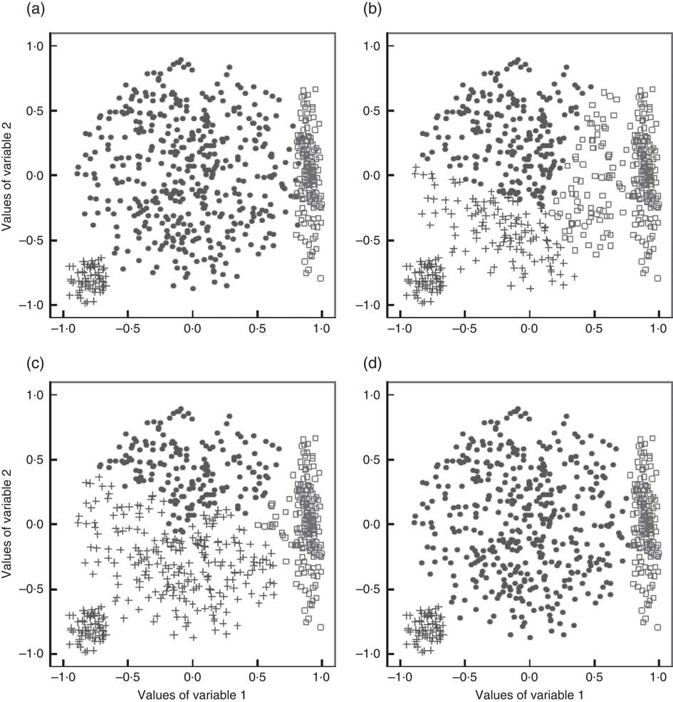
Fig. 1 A simulated two-dimensional data set with three clusters (represented by ●, □ and +) of variable volumes and shapes (‘true clusters’, a) as well as the clustering solutions obtained with the k-means algorithm (b), Ward’s method (c) and a Gaussian mixture model (GMM, d)
Gaussian mixture models
In order to overcome these limitations and to allow for clusters of variable volume, shape and orientation, Fraley and Raftery(
Reference Fraley and Raftery
9
) proposed a model-based approach using finite mixture models. This clustering approach assumes the observed data to be generated by a mixture of
![]() different p-dimensional normal distributions representing different clusters.
different p-dimensional normal distributions representing different clusters.
Let K be a non-observable random variable with values 1,...,g describing the true cluster membership and let X be a p-dimensional random vector describing the consumption frequencies of p food items. For each cluster k, the observations are assumed to be derived from a p-dimensional normal distribution. Then the probability density function of X, which is required to calculate the probability of an observation belonging to a given cluster, can be obtained as the weighted sum of all g normal distributions:
 $$f\left( {x\!\mid\!\psi } \right)=\mathop{\sum}\limits_{k=1}^g {\pi _{k} h(x\!\mid\!\mu _{k} ,\Sigma_{k} )} ,$$
where h(x|μ
k
, Σ
k
) denotes the p-dimensional normal probability density and $\psi =(\pi _{1} ,\,\ldots\pi _{g} ,\mu _{1} ,\ldots\mu _{g} ,\Sigma_{1} ,\ldots\Sigma_{g} )$
denotes the vector of all unknown parameters.
$\psi =(\pi _{1} ,\,\ldots\pi _{g} ,\mu _{1} ,\ldots\mu _{g} ,\Sigma_{1} ,\ldots\Sigma_{g} )$
denotes the vector of all unknown parameters.
![]() includes the mean vector
includes the mean vector
![]() p
, k=1,...,g, i.e. the mean consumption frequencies of the p food items in cluster k, the covariance matrix
p
, k=1,...,g, i.e. the mean consumption frequencies of the p food items in cluster k, the covariance matrix
![]() p×p
, i.e. the variances/covariances of the p food items in cluster k; as well as the mixing proportions π
k
, which can be interpreted as the probability of being assigned to cluster k.
p×p
, i.e. the variances/covariances of the p food items in cluster k; as well as the mixing proportions π
k
, which can be interpreted as the probability of being assigned to cluster k.
The unknown true parameter vector
![]() can be estimated by the maximum likelihood method, using the iterative Expectation-Maximization (EM) algorithm(
Reference Dempster, Laird and Rubin
12
) as described in McLachlan et al.(
Reference McLachlan and Chang
13
); see also Biernacki et al.(
Reference Biernacki, Celeux and Govaert
14
) for the generation of good initial values. A clustering solution can then be obtained by simply assigning each observation x
i
to the cluster
can be estimated by the maximum likelihood method, using the iterative Expectation-Maximization (EM) algorithm(
Reference Dempster, Laird and Rubin
12
) as described in McLachlan et al.(
Reference McLachlan and Chang
13
); see also Biernacki et al.(
Reference Biernacki, Celeux and Govaert
14
) for the generation of good initial values. A clustering solution can then be obtained by simply assigning each observation x
i
to the cluster $\mathord{\buildrel{\lower3pt\hbox{$\scriptscriptstyle\frown$}}\over k} _{i} $
to which it belongs with the highest probability, where the latter follows from Bayes’ Theorem. If there is more than one cluster fulfilling this property, x
i
is randomly assigned to one of these clusters.
$\mathord{\buildrel{\lower3pt\hbox{$\scriptscriptstyle\frown$}}\over k} _{i} $
to which it belongs with the highest probability, where the latter follows from Bayes’ Theorem. If there is more than one cluster fulfilling this property, x
i
is randomly assigned to one of these clusters.
In the context of GMM, the selection of an appropriate number of clusters
![]() may be treated as a model selection problem. Fraley and Raftery(
Reference Fraley and Raftery
9
) suggested to fit GMM with different numbers of clusters and to choose the model with the largest Bayesian Information Criterion.
may be treated as a model selection problem. Fraley and Raftery(
Reference Fraley and Raftery
9
) suggested to fit GMM with different numbers of clusters and to choose the model with the largest Bayesian Information Criterion.
One useful feature of GMM is the fact that they enable the user to place constraints on the geometrical properties of the clusters, e.g. to specify a desired degree of flexibility in terms of cluster volume, shape and orientation or to take advantage of pre-existing knowledge about these properties. This can be accomplished by different parameterizations of the covariance matrices Σ k and by restricting some of the parameters to be equal for all clusters k=1,...,g as described by Banfield and Raftery( Reference Banfield and Raftery 15 ). In the subsequent applications of the GMM, ten models putting different restrictions on the covariance matrix were estimated, including models with consumption frequency variances being allowed to vary within and/or across clusters as well as models (not) allowing for covariances among the consumption frequencies. Parameter estimation for these models is implemented in the R package mclust developed by Fraley and Raftery( Reference Fraley and Raftery 16 ).
Simulation study
The performances of the GMM approach, k-means and Ward’s method were first compared by means of a simulation study. All subsequent analyses were performed using the open-source statistical programming language R available at http://cran.r-project.org/( Reference Core Team 17 ).
Design
Three cluster geometries were investigated as illustrated in Fig. 2 based on an exemplary two-dimensional data set: spherical clusters with equal volume (Fig. 2(a)), ellipsoidal clusters with variable volume, shape and orientation (Fig. 2(b)) and cube-shaped clusters with equal volume and orientation (Fig. 2(c)). For each geometry, 10 000 data sets with twenty variables were generated using the function genRandomCluster() from the R package clusterGeneration( Reference Qiu and Joe 18 ). This function can be used to generate clustered data with a specified degree of between-cluster separation( Reference Qiu and Joe 19 ) ranging from −1 (no separation) to 1 (clearly separated clusters). A separation value of −0·1 was chosen in order to create strongly overlapping cluster structures which seemed to reflect the most realistic data structure.
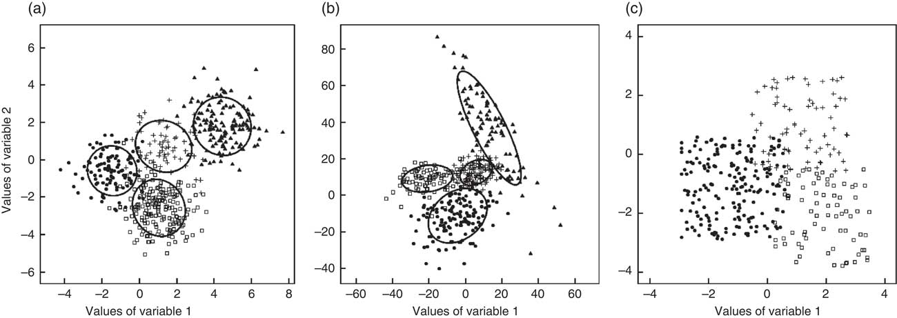
Fig. 2 Exemplary two-dimensional data set for each of the three cluster geometries: (a) spherical, equal volume; (b) variable volume, shape and orientation; and (c) cube-shaped, equal volume and orientation (●, □, ▲ and + represent different clusters)
For each data set, clustering solutions were obtained using the GMM with automatic model selection via the Bayesian Information Criterion (ten models putting different restrictions on the covariance matrix)( Reference Fraley and Raftery 16 ), the k-means algorithm (1000 starting values) and Ward’s method using SSQw as a measure for the cluster homogeneity. All algorithms were initialized with the true number of clusters. The obtained clustering solutions were compared with the true cluster structure using the adjusted Rand index (ARI)( Reference Hubert and Arabie 20 ), which measures the agreement of two clustering solutions. The values of the ARI range from −1 to 1 where a value of 1/−1 indicates perfect agreement/disagreement, with 0 being the expected value of the ARI if the observations are assigned to the clusters at random.
Results
Comparing the three clustering algorithms based on simulated data with spherical clusters of equal volume, the clustering solutions obtained from a GMM were more similar to the true cluster structure than those obtained from the k-means algorithm or Ward’s method for more than 72 % of all simulated data sets, as indicated in Table 1. For data sets with clusters of variable volume, shape and orientation, in more than 90 % of all cases the GMM achieved a higher agreement with the true cluster structure compared with the two heuristic methods.
Table 1 Comparison of pairs of clustering methods by how often each one achieved a higher agreement with the true cluster structure, based on 10 000 simulated data sets for each cluster geometry
GMM, Gaussian mixture model; ARI, adjusted Rand index.
* The ARI was used to measure the agreement with the true cluster structure.
Table 2 summarizes mean and percentile values of the ARI. The mean and median ARI of the clustering solutions obtained from the GMM are higher than those of the solutions obtained from the k-means algorithm or Ward’s method for all three cluster geometries, indicating better agreement of the GMM with the true cluster structure for the majority of simulated data sets.
Table 2 Comparison of the performance of the three clustering methods on 10 000 simulated data sets for each cluster geometry based on the ARI

GMM, Gaussian mixture model; ARI, adjusted Rand index.
* The ARI was used to measure the agreement with the true cluster structure.
Application to real data: FFQ data from the IDEFICS Study
All three clustering methods were applied to dietary data collected in the IDEFICS (Identification and Prevention of Dietary and Lifestyle-induced Health Effects in Children and Infants) Study to explore their performance in practice. IDEFICS is a European longitudinal multicentre study that aimed to investigate the causes of diet- and lifestyle-related diseases such as overweight and obesity in children and infants from eight European countries (Belgium, Cyprus, Estonia, Germany, Hungary, Italy, Spain and Sweden). In the present analysis, only the German IDEFICS sub-sample was considered. All study procedures were conducted according to the principles expressed in the Declaration of Helsinki and ethical approval was obtained from the local ethics committee. Parents provided written informed consent for all examinations. Each child was informed orally about the modules by field workers and asked for his/her consent immediately before examination. Details on the design and purpose of the IDEFICS Study can be obtained from Ahrens et al.( Reference Ahrens, Bammann and Siani 21 ).
Data and methods
During the German IDEFICS baseline survey conducted from 2007 to 2008, dietary data were assessed in 2014 children aged 2–9 years by means of a qualitative forty-five-item FFQ included in the IDEFICS Children’s Eating Habits Questionnaire (CEHQ-FFQ)( Reference Lanfer, Hebestreit and Ahrens 22 ). This paper-and-pencil based questionnaire was completed by proxies, mainly by parents. Usual ‘at home’ consumption frequencies of the forty-five food items were queried, i.e. meals not under parental control like school meals were not covered. The seven response categories ranged from ‘never/less than once a week’ up to ‘4 or more times per day’. Numerical values were assigned to convert the different answer categories into weekly consumption frequencies (0 up to 30 times/week). A detailed description of the CEHQ-FFQ is given elsewhere( Reference Lanfer, Hebestreit and Ahrens 22 – Reference Huybrechts, Börnhorst and Pala 24 ).
Height of the children was measured to the nearest 0·1 cm with a calibrated stadiometer (model: telescopic height measuring instruments SECA 225); body weight was measured in fasting state in light underwear on a calibrated scale accurate to 0·1 kg (model: electronic scale TANITA BC 420 SMA with adapter). BMI was calculated as weight divided by height squared and categorized according to the International Obesity Task Force criteria( Reference Cole, Bellizzi and Flegal 25 , Reference Cole, Flegal and Nicholls 26 ).
Observations with missing frequency values for more than five food items were excluded (n 223). In the remaining 1791 observations, missing values were imputed using the k-nearest-neighbour imputation approach which estimates missing values from the ten nearest observations with no missing values in the corresponding variables. The forty-five food items were aggregated into fifteen food groups (breakfast cereals, cheese, fast food, fruits, meat, meat alternatives, milk and yoghurt, refined cereals, sauces and butter, sweet drinks, sweet spread, sweets, vegetables, water, wholemeal bread). The aggregation was accomplished based on nutritional characteristics like sugar and fat content, where solid foods and drinks were distinguished. Furthermore, it was tried to avoid combining food items that might have contrary effects in terms of obesity risk. In order to get data that represent the composition of each child’s diet being at the same time easily comparable between children, the consumption frequencies of the derived food groups were divided by the sum of each child’s total consumption frequency over all food groups (relative frequencies). To achieve estimability of the formulated model, all variables except one can be explicitly modelled. Hence, water consumption frequency was dropped because it may contribute little to the clustering due to its small variability. Finally, the data were rescaled such that the variances of all remaining variables were equal to 1 to avoid artificially elongated clusters due to different variances of the marginal distributions.
In contrast to the simulation study, the number of clusters and the true cluster memberships are unknown when applying clustering methods to real data. Since in similar studies( Reference Newby and Tucker 6 ) clustering solutions with two to six clusters were obtained, solutions with two to six clusters were also estimated for the IDEFICS data using again GMM with automatic model selection via the Bayesian Information Criterion, k-means algorithm with 10 000 starting values and Ward’s method. For each number of clusters, the solutions obtained from the three clustering methods were compared using the ARI to assess their pairwise agreement. Furthermore, the interpretability of clustering solutions obtained with g=3 clusters was exemplarily examined to assess whether the clusters can indeed be regarded as representations of meaningful dietary patterns. This value of g was selected as the corresponding clustering solutions exhibited the highest pairwise similarities. Apart from the consumption frequencies, prevalences of overweight/obesity were compared between clusters to explore whether associations between dietary patterns and weight status are reasonable.
Results
The clustering solutions obtained for the CEHQ-FFQ data exhibit very little agreement between the three clustering methods as indicated in Table 3. For all g=2,…,6, the GMM solution is constantly more similar to the k-means solution than to the Ward solution. The best-fitting GMM for two to six clusters were those allowing the covariance matrix to be cluster dependent, i.e. those that allowed the variances of the food consumption frequencies to vary within and between clusters.
Table 3 Pairwise agreement between the clustering solutions obtained with the GMM, the k-means algorithm and Ward’s method assessed by the ARI

GMM, Gaussian mixture model; ARI, adjusted Rand index.
Comparing the three clustering methods, the solutions with g=3 clusters are most similar to each other. Here, the ARI is 0·47 comparing GMM v. k-means, 0·23 for GMM v. Ward and 0·20 for k-means v. Ward.
The clustering solutions with g=3 clusters obtained via the three clustering methods are summarized in Fig. 3. For each food item, the length of the corresponding bar represents the difference between the cluster-specific mean consumption frequency and the overall mean consumption frequency measured in units of overall standard deviations for this food item. All three methods identify one ‘non-processed’ cluster with higher-than-average consumption of fruits, vegetables and wholemeal bread and lower-than-average consumption of refined cereals, sweet drinks and fast food, represented by the left column in Fig. 3. The second cluster could be labelled as ‘balanced’ as there are no strongly preferred food items (middle column of Fig. 3). In this cluster, the consumption of sauces and butter, sweet drinks, meat and refined cereals is slightly higher than average, while the consumption frequencies of breakfast cereals, dairy products and fruits are slightly lower than average. The third ‘junk food’ cluster (right column of Fig. 3) consists of children with an increased consumption of fast food, breakfast cereals, meat alternatives and dairy products and a lower-than-average consumption of wholemeal bread, fruits and vegetables. The GMM and the k-means algorithm also find a preference for sweet snacks in the third cluster that is not present in the solution obtained from Ward’s method. For all three clustering methods, the prevalence of overweight/obesity is lower in the ‘non-processed’ cluster (13·9–14·5 % depending on the clustering method) compared with the ‘junk food’ cluster (15·7–16·3 %), which is an additional indicator of the reasonability of the exemplarily derived clustering solution (see Fig. 3).
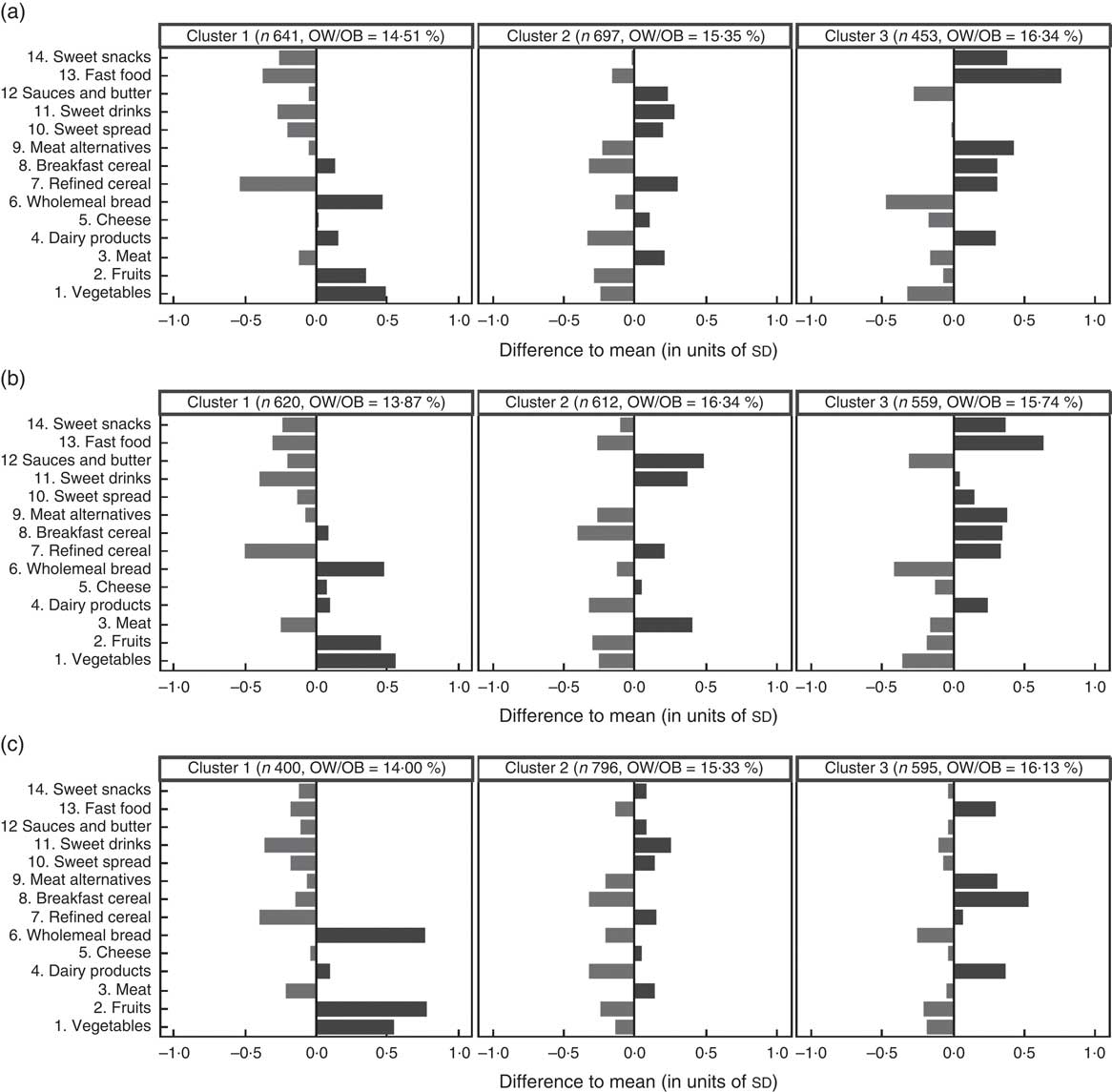
Fig. 3 Clustering solutions with three clusters obtained with (a) the Gaussian mixture model (GMM), (b) the k-means algorithm and (c) Ward’s method, based on the IDEFICS CEHQ-FFQ data (1791 children). For each food item, the lengths of the corresponding bars represent the difference between the cluster-specific mean consumption frequencies and the overall mean consumption frequencies in the sample, measured in units of overall standard deviations for the single food items. The number of observations and the percentage of overweight and obese( Reference Cole, Bellizzi and Flegal 25 ) (OW/OB) children are indicated for each cluster. IDEFICS, Identification and Prevention of Dietary- and Lifestyle-Induced Health Effects in Children and Infants; CEHQ, Children’s Eating Habits Questionnaire
Discussion
In the simulation study, the GMM outperforms the k-means algorithm and Ward’s method in the case of all three cluster geometries. Even though both heuristic methods are supposed to give particularly good results on data sets with spherical clusters of equal volume, they were still outperformed by the GMM on simulated data with this property. As expected, the outperformance of the GMM is most pronounced for data with clusters of variable volume, shape and orientation. Surprisingly, the GMM leads to better results than k-means and Ward’s method even for data sets with cube-shaped clusters despite the violation of its distributional assumptions.
Ward’s method performed poorly for many of the simulated data sets compared with both the GMM and k-means. This may be explained by the low degree of simulated cluster separation that leads to overlapping clusters in which neighbouring points often belong to different clusters. This could be problematic for an agglomerative hierarchical algorithm because fusions of clusters at an early stage of the algorithm are not reversible later on. If this is indeed the reason for the bad performance, Ward’s method might be inappropriate for finding clusters in FFQ data where strongly overlapping clusters are to be expected.
All results of the simulation study have been obtained under the assumption that the true number of clusters is known, while in general, this number is unknown. The choice of the most appropriate number of clusters is a crucial problem which is discussed elsewhere( Reference Fraley and Raftery 9 , Reference Milligan 11 , Reference Fransen, May and Stricker 27 ).
When exemplarily applying the clustering methods to real data, the low agreement of the clustering solutions according to the pairwise ARI values (Table 3) suggests that there might not be a manifest, easily identifiable cluster structure in the data. However, the results obtained for g=3 clusters summarized in Fig. 3 show that despite the low ARI values between these clustering solutions, all three methods find very similar dietary patterns with only minor differences in single food items. This finding suggests that the identified clusters might not just be artifacts of a particular clustering method, but may represent meaningful dietary patterns. The lower prevalence of overweight/obesity in the cluster labelled as ‘non-processed’ further underlines the reasonability of the clustering solutions. Nevertheless, several studies have revealed that self-reported dietary data are prone to measurement errors resulting e.g. from difficulties in estimation of consumption frequencies, memory errors or (intentional) misreporting( Reference Börnhorst, Huybrechts and Ahrens 28 , Reference Carroll, Freedman and Kipnis 29 ). In long-term dietary assessment instruments like FFQ as well as in proxy-reported data these problems may be even more pronounced( Reference Kipnis, Subar and Midthune 30 ). In the present analysis, the problem of under-/over-reporting may have been reduced by use of relative consumption frequencies as, for instance, a person consistently reporting lower consumption frequencies was related to his/her overall lower reported consumption frequency. When using absolute consumption frequencies in a preliminary analysis, one cluster with a higher-than-average consumption in all food groups and another cluster with a lower-than-average consumption in all food groups were identified. Both of these clusters were no longer present when using relative consumption frequencies. Nevertheless, the use of relative consumption frequencies may not reduce the problem of selective misreporting of certain foods. None of the applied clustering methods is able to account for such measurement errors. Hence, the identified dietary patterns should be interpreted with caution as they may only reflect reported but not necessarily true dietary intake.
Consistently with Fahey et al.( Reference Fahey, Thane and Bramwell 8 ), the best-fitting GMM for real FFQ data were those allowing the variances of the food consumption frequencies to vary within and between clusters. This suggests that the Ward’s method and k-means, which assume constant variances, may indeed not be optimal for dietary pattern analysis. The GMM is further advantageous as it gives a measure on the uncertainty of the cluster assignment, i.e. the probabilities of being assigned to the different clusters, and is able to account for correlated errors among variables (non-zero residual covariance) using specific parameterizations of the covariance matrix( Reference Fahey, Thane and Bramwell 8 ). However, a major difficulty in the application of GMM lies in potential violations of the distributional assumptions. Due to habitual non-consumption of certain foods, especially in children, many food groups exhibit a zero-inflated marginal distribution. This problem is illustrated in Fig. 4 based on two food items, dairy products and breakfast cereals. In this example, a large number of subjects reported a consumption frequency of zero for breakfast cereals leading to the huge number of observations clustered at the bottom line (x-axis) of Fig. 4. If there are food items with a high number of non-consumers, only models with strong geometric restrictions on the clusters can be fitted, for example those that assume clusters of equal volume or equal shape, making it impossible for the user to take full advantage of the flexibility of the GMM. In the present study we tried to overcome this problem by combining the food items of the FFQ into fewer and larger food groups. The investigation of different approaches to deal with zero inflation was beyond the scope of the paper. However, it should be kept in mind that not considering single food items but food groups results in a loss of information which is a limitation. Other possibilities to deal with zero inflation are: (i) the use of only those GMM with strong geometric restrictions on the clusters( Reference Banfield and Raftery 15 ); (ii) dichotomization of variables with a non-consumption higher than 50 %( Reference Fahey, Thane and Bramwell 8 , Reference Hunt and Jorgensen 31 , Reference Hunt and Jorgensen 32 ); (iii) the use of a truncated Gaussian mixture distribution( Reference Lee and Scott 33 ); (iv) the use of ‘a two-part model combining an indicator of food non-consumption with a continuous measurement for consumers’( Reference Gaio, da Costa and Santos 34 ); or (v) the application of multidimensional scaling to the data before clustering( Reference Oh and Raftery 35 ). Models like a truncated mixture model (iii) or a two-part model accounting for zero-inflated variables (iv) may be more realistic than the GMM but further increase the complexity of the model. Hence, future research should investigate whether these models lead to improved clustering solutions that would justify the increased complexity.

Fig. 4 Scatter plot of a two-dimensional projection of a sub-sample of the pre-processed IDEFICS CEHQ-FFQ data as an example of zero inflation in FFQ data. IDEFICS, Identification and Prevention of Dietary- and Lifestyle-Induced Health Effects in Children and Infants; CEHQ, Children’s Eating Habits Questionnaire
Conclusion
It was found that all three clustering methods are useful for the identification of meaningful dietary patterns by cluster analysis of FFQ data in practice. However, Ward’s method performed poorly in the simulation study and the EM algorithm can become numerically instable when fitting GMM with weak geometric restrictions on the clusters, making the application of these models more complex.
The promising results of the simulation study suggest that model-based clustering methods could provide better clustering solutions and thereby find more realistic dietary patterns than those identified with the standard methods used in most studies. The best-fitting GMM for real FFQ data were those allowing the variances of the food consumption frequencies to vary within and between clusters, which is not considered in Ward’s method and k-means. We therefore recommend the use of geometrically restricted GMM or alternatively the use of k-means, which often gives similar results but is more easily applicable.
In order to take full advantage of the higher flexibility provided by model-based clustering methods, the models need to be modified to account for zero inflation which is caused by habitual non-consumption of foods and currently complicates the application of GMM.
Acknowledgements
Financial support: This work was done as part of the IDEFICS Study (www.idefics.eu) and is published on behalf of its European Consortium. This work was supported by the European Community within the Sixth RTD Framework Programme Contract No. 016181 (FOOD). The European Community had no role in the design, analysis or writing of this article. Conflict of interest: None. Authorship: All authors contributed to conception and design, acquisition of data, analysis or interpretation of data. Each author has seen and approved the contents of the submitted manuscript. Final approval of the version published was given by all the authors. Ethics of human subject participation: All procedures in the IDEFICS Study were conducted according to the principles expressed in the Declaration of Helsinki and ethical approval was obtained from the local ethics committee. Parents provided written informed consent for all examinations.


