


1. Introduction
Cable-Driven Parallel Robots (CDPRs) are a class of parallel manipulators that utilize cables instead of rigid links to control the pose of the end-effector (EE). Each cable is spooled by a drum, which is part of a winch, typically mounted on an external rigid frame. The cable is routed from the drum to the EE through a pulley transmission system, where the final pulley is typically designed to swivel around an axis tangent to its groove, ensuring smooth guidance to the robot EE. By adjusting the cable lengths via servo-controlled winches, the EE can follow a desired trajectory and execute manipulation tasks. Cables exhibit a high payload-to-weight ratio since they are subjected only to tensile stresses, making CDPRs both lightweight and capable of handling significant loads [Reference Hu, Liu and Yuan1]. Another key advantage is the ease of deployment and reconfiguration. Indeed, the cable exit points from the frame can be changed online to adapt the CDPR workspace to the task to be executed [Reference Gagliardini, Caro, Gouttefarde and Girin2, Reference Gagliardini, Caro, Gouttefarde and Girin3] or to minimize power consumption [Reference Nguyen, Gouttefarde, Company and Pierrot4]. Alternatively, in the design phase, the CDPR geometry can be chosen to maximize stiffness [Reference Gagliardini, Gouttefarde, Caro, Ottaviano, Pelliccio and Gattulli5], minimize the maximum cable tension [Reference Hussein, Santos and Gouttefarde6], or increase dexterity [Reference Cheng and Lau7]. As cables impose unilateral constraints, CDPRs are usually equipped with more cables than the EE degrees of freedom (DOFs). In this configuration, if all cables always remain taut, the robot is overconstrained. Some CDPRs, called Underactuated CDPRs (UACDPRs), employ fewer cables than the EE degrees of freedom [Reference Ida’ and Carricato8], and they are inherently underconstrained. Consequently, the EE retains some DOFs even when all actuators are locked, and the EE pose cannot be assessed through direct kinematics only, since infinite poses are associated with the same set of cable lengths. Compared to overconstrained architectures, UACDPRs may offer specific advantages, depending on the application. For example, they improve obstacle avoidance, as fewer cables reduce the risk of interference with the environment, and fixed and operational costs decrease, as fewer actuators are required [Reference Angelini, Ida’, Bertin, Mantovani, Bazzi, Orassi and Carricato9].
Although reconfigurability makes CDPRs highly adaptable to varying tasks and environments, frequent reconfigurations present a major challenge: the need for frequent recalibration. At every reconfiguration, a calibration of the robot is needed to accurately determine the changes in the geometric (and possibly the inertial) model parameters, with the aim of enhancing the robot’s performance. Geometric calibration involves estimating the robot’s parameters by (i) performing some controlled motion of the EE to measure some internal variables and a ground truth (i.e., the robot pose) and (ii) minimizing the difference between the ground truth and its mathematical model (which explicitly depends on the measured internal variables) [Reference Khalil and Dombre10]. The conventional approach relies on external sensors to provide the ground truth, such as laser trackers [Reference dit Sandretto, Daney, Gouttefarde, Padois, Bidaud and Khatib11], which provide direct measurements of the EE pose relative to a fixed reference frame. In this case, the function to be minimized is the difference between measured and modeled EE poses [Reference dit Sandretto, Daney, Gouttefarde, Padois, Bidaud and Khatib11]. Alternatively, when no additional sensors other than the ones embedded in the robot kinematic chains are used for data acquisition, the procedure is called self-calibration, and it may be preferred to the conventional one, as it requires no additional cost for external sensors. A drawback is that calibration poses must be estimated alongside the robot’s geometric parameters. As a result, the number of unknowns increases while the number of independent equations remains the same. This generally reduces the accuracy of the estimated parameters, yielding poorer calibration results.
In CDPRs, most authors assume that direct or indirect measures of cable lengths and cable tensions are necessary for controlling the robot, as the former are used to derive motor setpoints, and the latter provide at least additional safety or additional capabilities to the robot. Typically, relative rotary encoders in the winch motors and load cells within the transmission are employed [Reference Ida’, Briot and Carricato12]. To compensate for cable elongation and provide a direct measure of cable length, laser distance sensors may also be used [Reference Martin, Fabritius, Stoll and Pott13]. Additionally, incremental encoders can be employed to measure the swivel angles in swivel pulleys [Reference Idá, Merlet, Carricato, Pott and Bruckmann14]. For a direct measure of the EE orientation, an Attitude and Heading Reference System (AHRS) can be integrated into the platform, thus improving pose estimation accuracy [Reference Gabaldo, Ida’, Carricato, Caro, Pott and Bruckmann15, Reference Gabaldo, Ida’ and Carricato16]. Finally, cable orientations can be estimated using accelerometers mounted on cables near their anchor points on the platform [Reference Merlet17].
Using relative sensors requires performing a procedure at every CDPR startup to determine their absolute reference values. This process, too, can be formulated as a self-calibration problem since it is equivalent to determining the initial pose of the EE and using the inverse geometric or static problem to determine the sensors’ reference values in the said pose.
In the past, several methods were proposed for the initial-pose self-calibration. Typically, the procedure is conducted offline using zero-order kinematics to model cable lengths based on the unknown calibration poses, measuring cable length variations, and minimizing the residuals [Reference dit Sandretto, Daney, Gouttefarde, Padois, Bidaud and Khatib11, Reference Lau, Gosselin, Cardou, Bruckmann and Pott18, Reference Wang, Caro, Point, Zeghloul, Laribi and Arsicault19]. Some approaches enhance accuracy by incorporating the swivel-pulley transmission model [Reference Zhang, Xie, Shao and Gosselin20] or leveraging swivel-angle measurements [Reference Idá, Merlet, Carricato, Pott and Bruckmann14]. More recent techniques exploit observability indices to enable online data selection for self-calibration [Reference Caverly, Bunker, Patel, Nguyen, Caro, Pott and Bruckmann21, Reference Caverly, Cheah, Bunker, Patel, Sexton and Nguyen22]. The initial-pose self-calibration is usually formulated as a Nonlinear Least Squares [Reference Idá, Merlet, Carricato, Pott and Bruckmann14, Reference Lau, Gosselin, Cardou, Bruckmann and Pott18–Reference Zhang, Xie, Shao and Gosselin20] or Nonlinear Weighted Least Squares (NWLS) [Reference dit Sandretto, Daney, Gouttefarde, Padois, Bidaud and Khatib11, Reference Caverly, Bunker, Patel, Nguyen, Caro, Pott and Bruckmann21, Reference Caverly, Cheah, Bunker, Patel, Sexton and Nguyen22] problem, where the unknowns include the initial values of the relative sensors and the measurement poses. The residual vector is composed of the difference between the quantities modeled by inverse kinematics (in the case of cable lengths or swivel angles) or statics (for cable tensions) and the measured ones. Even though effective solutions have been proposed for solving the initial-pose self-calibration problem of UACDPRs from a theoretical standpoint, there is still room for improvement in both accuracy and calibration speed. Current state-of-the-art methods require several minutes for automatic data acquisition [Reference Idá, Merlet, Carricato, Pott and Bruckmann14], and the initial estimated pose exhibits position and orientation errors of 2.5 cm and 2.2 degrees, respectively [Reference Zoffoli, Ida’, Carricato, Quaglia, Boschetti and Carbone23].
This paper extends the work presented in [Reference Zoffoli, Ida’, Carricato, Quaglia, Boschetti and Carbone23], where a rapid method for data acquisition and initial-pose self-calibration was introduced. This method aims at reducing data acquisition time, maintaining the same accuracy for the resulting initial pose compared to previous studies [Reference Idá, Merlet, Carricato, Pott and Bruckmann14]. While [Reference Zoffoli, Ida’, Carricato, Quaglia, Boschetti and Carbone23] achieved significant improvements in data acquisition efficiency, it requires operator intervention. In this study, we propose two novel data acquisition algorithms aimed at increasing the degree of automation while maintaining rapid and accurate self-calibration:
-
1. The first method involves moving the robot to static equilibrium poses, ensuring taut cables via low-level tension control, similarly to [Reference Idá, Merlet, Carricato, Pott and Bruckmann14]. Swivel-angle and cable-length variations are measured using incremental encoders, while an AHRS mounted on the EE captures orientation data. Load cells are used to measure cable tensions and regulate the motion of the UACDPR.
-
2. The second method solely relies on geometric constraints for self-calibration. It employs the same set of sensors as the first method but excludes load-cell measurements, using them only for EE motion control.
In both cases, the initial-pose estimation problem is formulated as a NWLS optimization problem, where the residuals to be minimized are the differences between the model-predicted values and actual sensor measurements. Experimental validation is conducted on a 4-cable UACDPR prototype, demonstrating the proposed methods’ effectiveness in reducing calibration time while maintaining accuracy.
The remainder of the paper is organized as follows. Section 2 introduces the kinematic and static models of a UACDPR. Section 3 presents the proposed self-calibration methodology, including data acquisition procedures. The experimental validation of the method on a 4-cable UACDPR is described in Section 4. Finally, conclusions and future research are provided in Section 5.
2. Kinematic and static models
A spatial UACDPR with a 6-degree-of-freedom (DoF) EE and
 $n$
cables is considered, with
$n$
cables is considered, with
 $n\lt 6$
. Cables are assumed to be massless and inextensible; therefore, no sagging or elastic phenomena are considered, and cables can be modeled as straight lines. This assumption is reasonable for small-scale UACDPRs, where the cable mass is negligible compared to the EE mass, and elastic deformations have a minimal effect on system behavior [Reference Fabritius, Miermeister, Kraus and Pott24]. Indicating the inertial frame with
$n\lt 6$
. Cables are assumed to be massless and inextensible; therefore, no sagging or elastic phenomena are considered, and cables can be modeled as straight lines. This assumption is reasonable for small-scale UACDPRs, where the cable mass is negligible compared to the EE mass, and elastic deformations have a minimal effect on system behavior [Reference Fabritius, Miermeister, Kraus and Pott24]. Indicating the inertial frame with
 $Oxyz$
and the frame attached to the EE with
$Oxyz$
and the frame attached to the EE with
 $Px'y'z'$
, the EE pose is defined by the position vector
$Px'y'z'$
, the EE pose is defined by the position vector
 $\boldsymbol{\mathbf{p}}$
of
$\boldsymbol{\mathbf{p}}$
of
 $P$
and the rotation matrix
$P$
and the rotation matrix
 ${\boldsymbol{\mathbf{R}}}({\boldsymbol{\mathbf{\epsilon }}})$
, where
${\boldsymbol{\mathbf{R}}}({\boldsymbol{\mathbf{\epsilon }}})$
, where
 ${\boldsymbol{\mathbf{\epsilon }}}=[\phi \; \theta \; \chi ]^T$
contains the Euler angles according to the
${\boldsymbol{\mathbf{\epsilon }}}=[\phi \; \theta \; \chi ]^T$
contains the Euler angles according to the
 $ZYX$
convention. Consequently, the generalized coordinates of the EE are
$ZYX$
convention. Consequently, the generalized coordinates of the EE are
 $\boldsymbol{\mathbf{\zeta }}=[\boldsymbol{\mathbf{p}}^T \; \boldsymbol{\mathbf{\epsilon }}^T]^T$
. Each cable is guided by a swiveling pulley into the workspace (Figure 1a). The
$\boldsymbol{\mathbf{\zeta }}=[\boldsymbol{\mathbf{p}}^T \; \boldsymbol{\mathbf{\epsilon }}^T]^T$
. Each cable is guided by a swiveling pulley into the workspace (Figure 1a). The
 $i$
-th cable enters the pulley groove at the fixed point
$i$
-th cable enters the pulley groove at the fixed point
 $D_i$
, exits at
$D_i$
, exits at
 $B_i$
, and is anchored to the platform at point
$B_i$
, and is anchored to the platform at point
 $A_i$
. To express the position of
$A_i$
. To express the position of
 $B_i$
in the inertial frame, we introduce a local reference frame
$B_i$
in the inertial frame, we introduce a local reference frame
 $D_ix_iy_iz_i$
, with constant unit vectors
$D_ix_iy_iz_i$
, with constant unit vectors
 ${\boldsymbol{\mathbf{i}}}_i$
,
${\boldsymbol{\mathbf{i}}}_i$
,
 ${\boldsymbol{\mathbf{j}}}_i$
,
${\boldsymbol{\mathbf{j}}}_i$
,
 ${\boldsymbol{\mathbf{k}}}_i$
(Figure 1b and 1c). The pulley geometry is modeled as in [Reference Zoffoli, Ida’, Carricato, Quaglia, Boschetti and Carbone23]. Each pulley of radius
${\boldsymbol{\mathbf{k}}}_i$
(Figure 1b and 1c). The pulley geometry is modeled as in [Reference Zoffoli, Ida’, Carricato, Quaglia, Boschetti and Carbone23]. Each pulley of radius
 $r_i$
and center
$r_i$
and center
 $C_i$
is tangent to the local axis
$C_i$
is tangent to the local axis
 $z_i$
at
$z_i$
at
 $D_i$
and swivels about
$D_i$
and swivels about
 $z_i$
by the angle
$z_i$
by the angle
 $\sigma _i$
. If the unit vector
$\sigma _i$
. If the unit vector
 ${\boldsymbol{\mathbf{u}}}_i$
points from
${\boldsymbol{\mathbf{u}}}_i$
points from
 $D_i$
to
$D_i$
to
 $C_i$
, and the unit vector
$C_i$
, and the unit vector
 ${\boldsymbol{\mathbf{w}}}_i$
is orthogonal to the pulley groove plane, then
${\boldsymbol{\mathbf{w}}}_i$
is orthogonal to the pulley groove plane, then
 ${\boldsymbol{\mathbf{w}}}_i={\boldsymbol{\mathbf{k}}}_i\times {\boldsymbol{\mathbf{u}}}_i$
. The tangency angle
${\boldsymbol{\mathbf{w}}}_i={\boldsymbol{\mathbf{k}}}_i\times {\boldsymbol{\mathbf{u}}}_i$
. The tangency angle
 $\psi _i$
defines the orientation of the unit vector
$\psi _i$
defines the orientation of the unit vector
 ${\boldsymbol{\mathbf{n}}}_i$
, which points from
${\boldsymbol{\mathbf{n}}}_i$
, which points from
 $C_i$
to
$C_i$
to
 $B_i$
. The unit vector along the
$B_i$
. The unit vector along the
 $i$
-th cable is
$i$
-th cable is
 ${\boldsymbol{\mathbf{t}}}_i={\boldsymbol{\mathbf{w}}}_i\times {\boldsymbol{\mathbf{n}}}_i$
. The aforementioned unit vectors can be described as:
${\boldsymbol{\mathbf{t}}}_i={\boldsymbol{\mathbf{w}}}_i\times {\boldsymbol{\mathbf{n}}}_i$
. The aforementioned unit vectors can be described as:
 \begin{equation} \begin{split} {\boldsymbol{\mathbf{u}}}_i &= \cos {\sigma _i}{\boldsymbol{\mathbf{i}}}_i+\sin {\sigma _i}{\boldsymbol{\mathbf{j}}}_i, \qquad {\boldsymbol{\mathbf{w}}}_i = -\sin {\sigma _i}{\boldsymbol{\mathbf{i}}}_i+\cos {\sigma _i}{\boldsymbol{\mathbf{j}}}_i, \\ {\boldsymbol{\mathbf{n}}}_i &= \cos {\psi _i}{\boldsymbol{\mathbf{u}}}_i+\sin {\psi _i}{\boldsymbol{\mathbf{k}}}_i, \qquad {\boldsymbol{\mathbf{t}}}_i = \sin {\psi _i}{\boldsymbol{\mathbf{u}}}_i-\cos {\psi _i}{\boldsymbol{\mathbf{k}}}_i . \end{split} \end{equation}
UACDPR geometric model.

The position of
 $D_i$
in the inertial frame
$D_i$
in the inertial frame
 $Oxyz$
is identified by the constant vector
$Oxyz$
is identified by the constant vector
 ${\boldsymbol{\mathbf{d}}}_i$
, while
${\boldsymbol{\mathbf{d}}}_i$
, while
 $B_i$
is described by
$B_i$
is described by
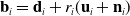 ${\boldsymbol{\mathbf{b}}}_i = {\boldsymbol{\mathbf{d}}}_i+r_i({\boldsymbol{\mathbf{u}}}_i+{\boldsymbol{\mathbf{n}}}_i)$
. The constant position of
${\boldsymbol{\mathbf{b}}}_i = {\boldsymbol{\mathbf{d}}}_i+r_i({\boldsymbol{\mathbf{u}}}_i+{\boldsymbol{\mathbf{n}}}_i)$
. The constant position of
 $A_i$
in the local frame
$A_i$
in the local frame
 $Px'y'z'$
is denoted by
$Px'y'z'$
is denoted by
 $^P{\boldsymbol{\mathbf{a}}}_i'$
, and in
$^P{\boldsymbol{\mathbf{a}}}_i'$
, and in
 $Oxyz$
is given by
$Oxyz$
is given by
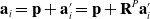 ${\boldsymbol{\mathbf{a}}}_i = {\boldsymbol{\mathbf{p}}}+{\boldsymbol{\mathbf{a}}}_i'={\boldsymbol{\mathbf{p}}}+{\boldsymbol{\mathbf{R}}}^P{\boldsymbol{\mathbf{a}}}_i'$
. Defining the vector
${\boldsymbol{\mathbf{a}}}_i = {\boldsymbol{\mathbf{p}}}+{\boldsymbol{\mathbf{a}}}_i'={\boldsymbol{\mathbf{p}}}+{\boldsymbol{\mathbf{R}}}^P{\boldsymbol{\mathbf{a}}}_i'$
. Defining the vector
 ${\boldsymbol{\mathbf{\varrho }}}_i=A_i-D_i={\boldsymbol{\mathbf{a}}}_i-{\boldsymbol{\mathbf{d}}}_i$
, and assuming that the cable remains coplanar with the swivel pulley, the resulting constraint is
${\boldsymbol{\mathbf{\varrho }}}_i=A_i-D_i={\boldsymbol{\mathbf{a}}}_i-{\boldsymbol{\mathbf{d}}}_i$
, and assuming that the cable remains coplanar with the swivel pulley, the resulting constraint is
 ${\boldsymbol{\mathbf{w}}}_i\cdot {\boldsymbol{\mathbf{\varrho }}}_i=0$
. From the latter, the swivel angle is found through inverse kinematics as:
${\boldsymbol{\mathbf{w}}}_i\cdot {\boldsymbol{\mathbf{\varrho }}}_i=0$
. From the latter, the swivel angle is found through inverse kinematics as:
 \begin{equation} \sigma _i = \mathrm{atan2}({\boldsymbol{\mathbf{j}}}_i\cdot {\boldsymbol{\mathbf{\varrho }}}_i,{\boldsymbol{\mathbf{i}}}_i\cdot {\boldsymbol{\mathbf{\varrho }}}_i). \end{equation}
Then, defining the cable vector as
 ${\boldsymbol{\mathbf{\rho }}}_i=A_i-B_i$
, and considering pulley kinematics, we obtain:
${\boldsymbol{\mathbf{\rho }}}_i=A_i-B_i$
, and considering pulley kinematics, we obtain:
 \begin{equation} {\boldsymbol{\mathbf{\rho }}}_i = {\boldsymbol{\mathbf{a}}}_i - {\boldsymbol{\mathbf{b}}}_i = {\boldsymbol{\mathbf{\varrho }}}_i-r_i({\boldsymbol{\mathbf{u}}}_i+{\boldsymbol{\mathbf{n}}}_i). \end{equation}
Since the cable is tangent to the pulley groove in
 $B_i$
, the tangency angle
$B_i$
, the tangency angle
 $\psi _i$
is determined using the geometric constraint
$\psi _i$
is determined using the geometric constraint
 ${\boldsymbol{\mathbf{n}}}_i\cdot {\boldsymbol{\mathbf{\rho }}}_i=0$
, leading to:
${\boldsymbol{\mathbf{n}}}_i\cdot {\boldsymbol{\mathbf{\rho }}}_i=0$
, leading to:
 \begin{equation} \psi _i=2\arctan \left (\frac {\varrho _{k_i}}{\varrho _{u_i}}+\sqrt {\left (\frac {\varrho _{k_i}}{\varrho _{u_i}}\right )^2+1-\frac {2r_i}{\varrho _{u_i}}}\right ), \end{equation}
where
 $\varrho _{k_i}={\boldsymbol{\mathbf{\varrho }}}_i\cdot {\boldsymbol{\mathbf{k}}}_i$
and
$\varrho _{k_i}={\boldsymbol{\mathbf{\varrho }}}_i\cdot {\boldsymbol{\mathbf{k}}}_i$
and
 $\varrho _{u_i}={\boldsymbol{\mathbf{\varrho }}}_i\cdot {\boldsymbol{\mathbf{u}}}_i$
. The total cable length
$\varrho _{u_i}={\boldsymbol{\mathbf{\varrho }}}_i\cdot {\boldsymbol{\mathbf{u}}}_i$
. The total cable length
 $l_i$
(
$l_i$
(
 $\gt 0$
) consists of the rectilinear segment
$\gt 0$
) consists of the rectilinear segment
 $\|{\boldsymbol{\mathbf{\rho }}}_i\|$
and the arc
$\|{\boldsymbol{\mathbf{\rho }}}_i\|$
and the arc
 $\widehat {D_{i} B_{i}}$
wrapped around the pulley:
$\widehat {D_{i} B_{i}}$
wrapped around the pulley:
 \begin{equation} l_i = \| {\boldsymbol{\mathbf{\rho }}}_i \|+r_i(\pi -\psi _i) . \end{equation}
The CDPR static model is obtained from the mechanical equilibrium of the EE. The model is formulated under the assumption that all cables remain taut and that gravity is the only external force acting on the EE, so that:
 \begin{equation} \mathbf{\Xi }^T\boldsymbol{\mathbf{\tau }} = \mathbf{f}, \quad \mathrm{with}\quad \mathbf{f}=\begin{bmatrix} \mathbf{g} \\ \mathbf{s}'\times \mathbf{g} \end{bmatrix}, \end{equation}
where
 $\mathbf{g}=[0, 0, -mg]^T$
,
$\mathbf{g}=[0, 0, -mg]^T$
,
 $m$
is the EE mass,
$m$
is the EE mass,
 $g$
is the gravitational acceleration,
$g$
is the gravitational acceleration,
 $\mathbf{s}'$
is the position vector from
$\mathbf{s}'$
is the position vector from
 $P$
to the center of mass
$P$
to the center of mass
 $G$
, and
$G$
, and
 $\boldsymbol{\mathbf{\tau }}\in \mathbb{R}^n$
is the array of cable tensions.
$\boldsymbol{\mathbf{\tau }}\in \mathbb{R}^n$
is the array of cable tensions.
 $\boldsymbol{\mathbf{\Xi }}^T\in \mathbb{R}^{6\times n}$
is the structure matrix, which relates cable tensions to forces and torques on the EE, and is computed as in [Reference Idà, Briot and Carricato25]:
$\boldsymbol{\mathbf{\Xi }}^T\in \mathbb{R}^{6\times n}$
is the structure matrix, which relates cable tensions to forces and torques on the EE, and is computed as in [Reference Idà, Briot and Carricato25]:
 \begin{equation} \boldsymbol{\mathbf{\xi }}_{i}=\begin{bmatrix} \mathbf{t}_i\\ {\boldsymbol{\mathbf{a}}}_i'\times \mathbf{t}_i \end{bmatrix} , \qquad \boldsymbol{\mathrm{\Xi }}^T = [\boldsymbol{\mathbf{\xi }}_{1},\ldots ,\boldsymbol{\mathbf{\xi }}_{n}] . \end{equation}
3. Self-calibration and data-acquisition algorithms
In previous studies [Reference dit Sandretto, Daney, Gouttefarde, Padois, Bidaud and Khatib11, Reference Lau, Gosselin, Cardou, Bruckmann and Pott18–Reference Zhang, Xie, Shao and Gosselin20], motor encoders have been used as primary sensors for CDPR self-calibration. For overconstrained CDPRs, load cells have been shown to be effective for this purpose too [Reference Miermeister, Pott, Lenarcic and Husty26, Reference Liu, Qin, Gao, Sun, Huang and Deng27].
In this work, as in [Reference Zoffoli, Ida’, Carricato, Quaglia, Boschetti and Carbone23], we consider UACDPRs equipped with multiple internal sensors for state estimation and motion control. In particular, indicating the measured quantities with the superscript
 $(\cdot )^*$
, an incremental encoder on the
$(\cdot )^*$
, an incremental encoder on the
 $i$
-th swivel pulley measures variations in the swivel angles
$i$
-th swivel pulley measures variations in the swivel angles
 $\Delta \sigma _i^*$
relative to the angular position at startup
$\Delta \sigma _i^*$
relative to the angular position at startup
 $\sigma _{i,0}$
. An AHRS, rigidly attached to the platform with its reference frame coincident with the EE mobile frame, provides roll and pitch angles (
$\sigma _{i,0}$
. An AHRS, rigidly attached to the platform with its reference frame coincident with the EE mobile frame, provides roll and pitch angles (
 $\phi ^*$
and
$\phi ^*$
and
 $\theta ^*$
) relative to a local-earth frame (east-north-up) coinciding with
$\theta ^*$
) relative to a local-earth frame (east-north-up) coinciding with
 $Oxyz$
, as well as the relative yaw variation
$Oxyz$
, as well as the relative yaw variation
 $\Delta \chi ^*$
from the startup configuration
$\Delta \chi ^*$
from the startup configuration
 $\chi _0$
. Additionally, an incremental encoder in the winch motor tracks the motor angle displacement
$\chi _0$
. Additionally, an incremental encoder in the winch motor tracks the motor angle displacement
 $\Delta \theta _{m,i}^*$
relative to the startup value
$\Delta \theta _{m,i}^*$
relative to the startup value
 $\theta _{m,i,0}$
. When the
$\theta _{m,i,0}$
. When the
 $i$
-th winch is designed with a constant and known transmission ratio
$i$
-th winch is designed with a constant and known transmission ratio
 $K$
between cable-length variation and motor displacement (as assumed here), the cable-length variation can be indirectly estimated as
$K$
between cable-length variation and motor displacement (as assumed here), the cable-length variation can be indirectly estimated as
 $\Delta l_i^* = K\Delta \theta _{m,i}^*$
[Reference Ida’ and Mattioni28]. Finally, a load cell is integrated into each transmission to measure the
$\Delta l_i^* = K\Delta \theta _{m,i}^*$
[Reference Ida’ and Mattioni28]. Finally, a load cell is integrated into each transmission to measure the
 $i$
-th cable tension
$i$
-th cable tension
 $\tau _i^*$
.
$\tau _i^*$
.
The choice of this sensor set is based on three main reasons. First, previous studies [Reference Gabaldo, Ida’, Carricato, Caro, Pott and Bruckmann15, Reference Gabaldo, Ida’ and Carricato16] demonstrated the effectiveness of incremental encoders and AHRSs for accurate pose estimation in UACDPRs. Therefore, it is reasonable to adopt this configuration as the available internal sensor suite, since these sensors will also be used for state estimation after calibration. Second, cable-tension measurements, whether obtained directly through load cells or estimated from motor currents [Reference Guagliumi, Berti, Monti, Fabritius, Martin and Carricato29], are typically employed for control and safety purposes, such as ensuring that all cables remain taut during operation. Since these measurements are already available in the control loop, they can be naturally included in the self-calibration formulation to enhance pose estimation accuracy. Third, the use of multiple sensors helps mitigate errors introduced by the simplified modeling assumptions described in Section 2, where cables are modeled as straight lines and the swivel pulleys are assumed to remain coplanar with the corresponding cable directions.
If other internal sensing systems are available, such as laser distance sensors for directly measuring cable elongation [Reference Martin, Fabritius, Stoll and Pott13], they can be easily integrated into our approach, which is fully general. Indeed, including additional sensors may yield faster and more accurate results.
3.1. Self-calibration algorithms
At a generic EE pose
 ${\boldsymbol{\mathbf{\zeta }}}_i$
, if the constraints imposed by the swivel pulleys and the cables on the moving platform are active,Footnote
1
the relationships between modeled and measured quantities for cable lengths, swivel angles, and orientation angles can be expressed as:
${\boldsymbol{\mathbf{\zeta }}}_i$
, if the constraints imposed by the swivel pulleys and the cables on the moving platform are active,Footnote
1
the relationships between modeled and measured quantities for cable lengths, swivel angles, and orientation angles can be expressed as:
 \begin{align} {\boldsymbol{\mathbf{l}}}({\boldsymbol{\mathbf{\zeta }}}_i) &= {\boldsymbol{\mathbf{l}}}_0 + \Delta {\boldsymbol{\mathbf{l}}}_i^*, \quad {\boldsymbol{\mathbf{\sigma }}}({\boldsymbol{\mathbf{\zeta }}}_i) = {\boldsymbol{\mathbf{\sigma }}}_0+\Delta {\boldsymbol{\mathbf{\sigma }}}_i^*, \\[-12pt] \nonumber \end{align}
 \begin{align} \phi ({\boldsymbol{\mathbf{\zeta }}}_i) = &\phi _i^*, \quad \theta ({\boldsymbol{\mathbf{\zeta }}}_i) = \theta _i^*, \quad \chi ({\boldsymbol{\mathbf{\zeta }}}_i) = {\boldsymbol{\mathbf{\chi }}}_0+\Delta \chi _i^*. \\[12pt] \nonumber \end{align}
In Eqs. (8) and (9), the modeled cable-length array
 ${\boldsymbol{\mathbf{l}}}({\boldsymbol{\mathbf{\zeta }}}_i)$
and swivel-angle array
${\boldsymbol{\mathbf{l}}}({\boldsymbol{\mathbf{\zeta }}}_i)$
and swivel-angle array
 ${\boldsymbol{\mathbf{\sigma }}}({\boldsymbol{\mathbf{\zeta }}}_i)$
are obtained through inverse kinematics, namely through Eqs. (5) and (2), whereas the modeled Euler angles
${\boldsymbol{\mathbf{\sigma }}}({\boldsymbol{\mathbf{\zeta }}}_i)$
are obtained through inverse kinematics, namely through Eqs. (5) and (2), whereas the modeled Euler angles
 $\phi ({\boldsymbol{\mathbf{\zeta }}}_i)$
,
$\phi ({\boldsymbol{\mathbf{\zeta }}}_i)$
,
 $\theta ({\boldsymbol{\mathbf{\zeta }}}_i)$
, and
$\theta ({\boldsymbol{\mathbf{\zeta }}}_i)$
, and
 $\chi ({\boldsymbol{\mathbf{\zeta }}}_i)$
are the orientation components of the pose
$\chi ({\boldsymbol{\mathbf{\zeta }}}_i)$
are the orientation components of the pose
 ${\boldsymbol{\mathbf{\zeta }}}_i$
. The measured quantities in Eqs. (8) and (9), instead, depend on the directly measured data
${\boldsymbol{\mathbf{\zeta }}}_i$
. The measured quantities in Eqs. (8) and (9), instead, depend on the directly measured data
 $\Delta \boldsymbol{\mathbf{l}}^*$
,
$\Delta \boldsymbol{\mathbf{l}}^*$
,
 $\Delta \boldsymbol{\mathbf{\sigma }}^*$
,
$\Delta \boldsymbol{\mathbf{\sigma }}^*$
,
 $\phi ^*$
,
$\phi ^*$
,
 $\theta ^*$
,
$\theta ^*$
,
 $\Delta \chi ^*$
and on the initial values
$\Delta \chi ^*$
and on the initial values
 $\boldsymbol{\mathbf{l}}_0$
,
$\boldsymbol{\mathbf{l}}_0$
,
 $\boldsymbol{\mathbf{\sigma }}_0$
,
$\boldsymbol{\mathbf{\sigma }}_0$
,
 $\chi _0$
.
$\chi _0$
.
Additionally, if the generic pose
 ${\boldsymbol{\mathbf{\zeta }}}_i$
is a static equilibrium one, the relation between the modeled and measured cable tensions is given by:
${\boldsymbol{\mathbf{\zeta }}}_i$
is a static equilibrium one, the relation between the modeled and measured cable tensions is given by:
 \begin{equation} {\boldsymbol{\mathbf{\tau }}}({\boldsymbol{\mathbf{\zeta }}}_i) = {\boldsymbol{\mathbf{\tau }}}_i^*, \end{equation}
where the modeled tension array
 ${\boldsymbol{\mathbf{\tau }}}({\boldsymbol{\mathbf{\zeta }}}_i)$
can be computed from (6) through a generic left inverse
${\boldsymbol{\mathbf{\tau }}}({\boldsymbol{\mathbf{\zeta }}}_i)$
can be computed from (6) through a generic left inverse
 ${\boldsymbol{\mathbf{\Xi }}}^{-T}$
of the structure matrix:
${\boldsymbol{\mathbf{\Xi }}}^{-T}$
of the structure matrix:
 \begin{equation} {\boldsymbol{\mathbf{\tau }}}({\boldsymbol{\mathbf{\zeta }}}_i) = {\boldsymbol{\mathbf{\Xi }}}^{-T}({\boldsymbol{\mathbf{\zeta }}}_i){\boldsymbol{\mathbf{f}}}({\boldsymbol{\mathbf{\zeta }}}_i). \end{equation}
To define a specific inverse of
 ${\boldsymbol{\mathbf{\Xi }}}^T$
, we partition it into two blocks, namely
${\boldsymbol{\mathbf{\Xi }}}^T$
, we partition it into two blocks, namely
 ${\boldsymbol{\mathbf{\Xi }}}^T = [{\boldsymbol{\mathbf{\Xi }}}_{c} \; {\boldsymbol{\mathbf{\Xi }}}_{f}]^T$
, where
${\boldsymbol{\mathbf{\Xi }}}^T = [{\boldsymbol{\mathbf{\Xi }}}_{c} \; {\boldsymbol{\mathbf{\Xi }}}_{f}]^T$
, where
 ${\boldsymbol{\mathbf{\Xi }}}_c \in \mathbb{R}^{n\times n}$
and
${\boldsymbol{\mathbf{\Xi }}}_c \in \mathbb{R}^{n\times n}$
and
 ${\boldsymbol{\mathbf{\Xi }}}_f\in \mathbb{R}^{n\times (6-n)}$
. The corresponding left inverse is given by:
${\boldsymbol{\mathbf{\Xi }}}_f\in \mathbb{R}^{n\times (6-n)}$
. The corresponding left inverse is given by:
 \begin{equation} {\boldsymbol{\mathbf{\Xi }}}^{-T} = \begin{bmatrix} {\boldsymbol{\mathbf{\Xi }}}^{-T}_c & {\boldsymbol{\mathbf{0}}}_{n\times (6-n)} \end{bmatrix}, \end{equation}
where
 ${\boldsymbol{\mathbf{0}}}_{n\times (6-n)}$
is a null matrix with
${\boldsymbol{\mathbf{0}}}_{n\times (6-n)}$
is a null matrix with
 $n$
rows and
$n$
rows and
 $(6-n)$
columns.
$(6-n)$
columns.
In conventional formulations (e.g., [Reference dit Sandretto, Daney, Gouttefarde, Padois, Bidaud and Khatib11, Reference Idá, Merlet, Carricato, Pott and Bruckmann14, Reference Lau, Gosselin, Cardou, Bruckmann and Pott18–Reference Zhang, Xie, Shao and Gosselin20, Reference Caverly, Cheah, Bunker, Patel, Sexton and Nguyen22]), the array of unknowns
 $\boldsymbol{\mathbf{X}}$
in the initial-pose self-calibration problem, typically includes the initial values
$\boldsymbol{\mathbf{X}}$
in the initial-pose self-calibration problem, typically includes the initial values
 ${\boldsymbol{\mathbf{l}}}_0$
,
${\boldsymbol{\mathbf{l}}}_0$
,
 ${\boldsymbol{\mathbf{\sigma }}}_0$
,
${\boldsymbol{\mathbf{\sigma }}}_0$
,
 $\chi _0$
, as well as multiple measurement poses
$\chi _0$
, as well as multiple measurement poses
 ${\boldsymbol{\mathbf{Z}}} = [{\boldsymbol{\mathbf{\zeta }}}_1^T,\ldots ,{\boldsymbol{\mathbf{\zeta }}}_k^T]^T$
. With a sufficient number of measurement poses
${\boldsymbol{\mathbf{Z}}} = [{\boldsymbol{\mathbf{\zeta }}}_1^T,\ldots ,{\boldsymbol{\mathbf{\zeta }}}_k^T]^T$
. With a sufficient number of measurement poses
 $k$
, an overdetermined nonlinear system of equations composed by Eqs. (8), (9), and (10) can be established, which is desirable to reduce the impact of measurement errors. In contrast, in our approach, the initial values
$k$
, an overdetermined nonlinear system of equations composed by Eqs. (8), (9), and (10) can be established, which is desirable to reduce the impact of measurement errors. In contrast, in our approach, the initial values
 ${\boldsymbol{\mathbf{l}}}_0$
,
${\boldsymbol{\mathbf{l}}}_0$
,
 ${\boldsymbol{\mathbf{\sigma }}}_0$
, and
${\boldsymbol{\mathbf{\sigma }}}_0$
, and
 $\chi _0$
are reformulated as explicit functions of the initial EE pose
$\chi _0$
are reformulated as explicit functions of the initial EE pose
 ${\boldsymbol{\mathbf{\zeta }}}_0$
, using the kinematic relations in Eqs. (5) and (2). This reformulation shifts the estimation task from identifying the initial value of the measured quantities to estimating the initial EE pose (together with the measurement poses). The residuals for the
${\boldsymbol{\mathbf{\zeta }}}_0$
, using the kinematic relations in Eqs. (5) and (2). This reformulation shifts the estimation task from identifying the initial value of the measured quantities to estimating the initial EE pose (together with the measurement poses). The residuals for the
 $i$
-th measurement equilibrium pose become:
$i$
-th measurement equilibrium pose become:
 \begin{equation} \begin{aligned}&{\boldsymbol{\mathbf{F}}}_{\tau ,i}=\boldsymbol{\mathbf{\tau }}(\boldsymbol{\mathbf{\zeta }}_i)-\boldsymbol{\mathbf{\tau }}^*_i, \\ &{\boldsymbol{\mathbf{F}}}_{l,i}=\boldsymbol{\mathbf{l}}(\boldsymbol{\mathbf{\zeta }}_i) - \boldsymbol{\mathbf{l}}_0(\boldsymbol{\mathbf{\zeta }}_0)-\Delta \boldsymbol{\mathbf{l}}^*_i,\\ &{\boldsymbol{\mathbf{F}}}_{\sigma ,i}=\boldsymbol{\mathbf{\sigma }}(\boldsymbol{\mathbf{\zeta }}_i)-\boldsymbol{\mathbf{\sigma }}_0(\boldsymbol{\mathbf{\zeta }}_0) -\Delta \boldsymbol{\mathbf{\sigma }}^*_i,\end{aligned} \qquad {\boldsymbol{\mathbf{F}}}_{\epsilon ,i}=\begin{bmatrix}\phi (\boldsymbol{\mathbf{\zeta }}_i)-\phi ^*_i \\[4pt] \theta (\boldsymbol{\mathbf{\zeta }}_i)-\theta ^*_i \\[4pt] \chi (\boldsymbol{\mathbf{\zeta }}_i)-\chi _0(\boldsymbol{\mathbf{\zeta }}_0)-\Delta \chi ^*_i \end{bmatrix} \end{equation}
Therefore, the actual calibration task becomes the estimation of
 $\boldsymbol{\mathbf{\zeta }}_0$
, from which the initial values of the measured quantities can be derived via inverse kinematics. This strategy reduces the number of unknowns and thus increases the equation-to-unknown ratio. Assuming that the modeling error introduced by inverse kinematics is negligible, this leads to improved computational efficiency and fewer measurements to obtain a desired accuracy in the estimation. Therefore, the same approach as in [Reference Zoffoli, Ida’, Carricato, Quaglia, Boschetti and Carbone23] is used, where the array of unknowns
$\boldsymbol{\mathbf{\zeta }}_0$
, from which the initial values of the measured quantities can be derived via inverse kinematics. This strategy reduces the number of unknowns and thus increases the equation-to-unknown ratio. Assuming that the modeling error introduced by inverse kinematics is negligible, this leads to improved computational efficiency and fewer measurements to obtain a desired accuracy in the estimation. Therefore, the same approach as in [Reference Zoffoli, Ida’, Carricato, Quaglia, Boschetti and Carbone23] is used, where the array of unknowns
 ${\boldsymbol{\mathbf{X}}}=[{\boldsymbol{\mathbf{\zeta }}}_0^T,{\boldsymbol{\mathbf{\zeta }}}_1^T,\ldots ,{\boldsymbol{\mathbf{\zeta }}}_k^T]^T\in \mathbb{R}^{6(k+1)}$
is composed by the initial pose
${\boldsymbol{\mathbf{X}}}=[{\boldsymbol{\mathbf{\zeta }}}_0^T,{\boldsymbol{\mathbf{\zeta }}}_1^T,\ldots ,{\boldsymbol{\mathbf{\zeta }}}_k^T]^T\in \mathbb{R}^{6(k+1)}$
is composed by the initial pose
 ${\boldsymbol{\mathbf{\zeta }}}_0$
and
${\boldsymbol{\mathbf{\zeta }}}_0$
and
 $k$
measurement configurations.
$k$
measurement configurations.
Two self-calibration algorithms are considered, each utilizing a different sensor set and indexed by
 $j \in \{\tau l\sigma \epsilon , l\sigma \epsilon \}$
. The first algorithm (
$j \in \{\tau l\sigma \epsilon , l\sigma \epsilon \}$
. The first algorithm (
 $j = \tau l\sigma \epsilon$
) uses all the available sensors, including those measuring cable tensions, swivel-angle variations, cable-length variations, roll, pitch, and yaw variations. The second algorithm (
$j = \tau l\sigma \epsilon$
) uses all the available sensors, including those measuring cable tensions, swivel-angle variations, cable-length variations, roll, pitch, and yaw variations. The second algorithm (
 $j=l\sigma \epsilon$
) excludes cable tension measurements and only relies on the other sensors. The motivation for considering these two algorithms lies in the set of equations available for the self-calibration process, which directly influences the data acquisition strategy. On the one hand, maximizing the ratio between the number of equations and the number of unknowns is desirable, and this can be achieved by incorporating all available sensors, including load cells. However, using load cell measurements inherently requires relying on static equilibrium equations, as dynamic equations would introduce additional unknowns (namely, pose derivatives), counteracting the goal of maximizing the equation-to-unknowns ratio. As a consequence, the calibration process must rely on static EE poses, potentially leading to longer data acquisition times due to the need for self-energy dissipation. Excluding load cell measurements simplifies the calibration process by relying only on geometric constraints, as shown in [Reference Zoffoli, Ida’, Carricato, Quaglia, Boschetti and Carbone23]. This allows for rapid movements and faster data acquisition at the cost of a lower equation-to-unknowns ratio, which may, in turn, reduce the accuracy of calibration results.
$j=l\sigma \epsilon$
) excludes cable tension measurements and only relies on the other sensors. The motivation for considering these two algorithms lies in the set of equations available for the self-calibration process, which directly influences the data acquisition strategy. On the one hand, maximizing the ratio between the number of equations and the number of unknowns is desirable, and this can be achieved by incorporating all available sensors, including load cells. However, using load cell measurements inherently requires relying on static equilibrium equations, as dynamic equations would introduce additional unknowns (namely, pose derivatives), counteracting the goal of maximizing the equation-to-unknowns ratio. As a consequence, the calibration process must rely on static EE poses, potentially leading to longer data acquisition times due to the need for self-energy dissipation. Excluding load cell measurements simplifies the calibration process by relying only on geometric constraints, as shown in [Reference Zoffoli, Ida’, Carricato, Quaglia, Boschetti and Carbone23]. This allows for rapid movements and faster data acquisition at the cost of a lower equation-to-unknowns ratio, which may, in turn, reduce the accuracy of calibration results.
In both algorithms, the initial-pose self-calibration problem is formulated as a NWLS optimization:
 \begin{equation} \mathbf{X}_{sol,j} = \arg \min _{\mathbf{X}}h_j(\mathbf{X}), \quad \mathrm{with} \quad h_j(\mathbf{X})=\frac {1}{2}\mathbf{F}_j^T\mathbf{W}_j\mathbf{F}_j . \end{equation}
The residual array
 ${\boldsymbol{\mathbf{F}}}_j$
is composed of different combinations of residual blocks depending on the sensor set used :
${\boldsymbol{\mathbf{F}}}_j$
is composed of different combinations of residual blocks depending on the sensor set used :
 \begin{equation} {\boldsymbol{\mathbf{F}}}_{\tau l \sigma \epsilon }=[{\boldsymbol{\mathbf{F}}}_{\tau }^T \; {\boldsymbol{\mathbf{F}}}_{l}^T \; {\boldsymbol{\mathbf{F}}}_{\sigma }^T \; {\boldsymbol{\mathbf{F}}}_{\epsilon }^T]^T\in \mathbb{R}^{k(3n+3)}, \qquad {\boldsymbol{\mathbf{F}}}_{l \sigma \epsilon }=[{\boldsymbol{\mathbf{F}}}_{l}^T \; {\boldsymbol{\mathbf{F}}}_{\sigma }^T \; {\boldsymbol{\mathbf{F}}}_{\epsilon }^T]^T\in \mathbb{R}^{k(2n+3)}. \end{equation}
Each residual block is constructed by vertically stacking the corresponding single-pose residuals defined in Eq. (13) across all
 $k$
measurement configurations:
$k$
measurement configurations:
 \begin{equation} \begin{split} {\boldsymbol{\mathbf{F}}}_\sigma &= \begin{bmatrix} {\boldsymbol{\mathbf{\sigma }}}({\boldsymbol{\mathbf{\zeta }}}_1)-{\boldsymbol{\mathbf{\sigma }}}_0({\boldsymbol{\mathbf{\zeta }}}_0)-\Delta {\boldsymbol{\mathbf{\sigma }}}_1^* \\[3pt] \vdots \\[3pt] {\boldsymbol{\mathbf{\sigma }}}({\boldsymbol{\mathbf{\zeta }}}_k)-{\boldsymbol{\mathbf{\sigma }}}_0({\boldsymbol{\mathbf{\zeta }}}_0)-\Delta {\boldsymbol{\mathbf{\sigma }}}_k^* \end{bmatrix}\in \mathbb{R}^{kn}, \; {\boldsymbol{\mathbf{F}}}_\epsilon = \begin{bmatrix} \phi ({\boldsymbol{\mathbf{\zeta }}}_1)-\phi _1^* \\[3pt] \theta ({\boldsymbol{\mathbf{\zeta }}}_1)-\theta _1^* \\[3pt] \chi ({\boldsymbol{\mathbf{\zeta }}}_1)-\chi _0({\boldsymbol{\mathbf{\zeta }}}_0)-\Delta \chi _1^* \\[3pt] \vdots \\[3pt] \phi ({\boldsymbol{\mathbf{\zeta }}}_k)-\phi _k^* \\[3pt] \theta ({\boldsymbol{\mathbf{\zeta }}}_k)-\theta _k^* \\[3pt] \chi ({\boldsymbol{\mathbf{\zeta }}}_k)-\chi _0({\boldsymbol{\mathbf{\zeta }}}_0)-\Delta \chi _k^* \end{bmatrix}\in \mathbb{R}^{3k}, \\[3pt] {\boldsymbol{\mathbf{F}}}_l &= \begin{bmatrix} {\boldsymbol{\mathbf{l}}}({\boldsymbol{\mathbf{\zeta }}}_1)-{\boldsymbol{\mathbf{l}}}_0({\boldsymbol{\mathbf{\zeta }}}_0)-\Delta {\boldsymbol{\mathbf{l}}}_1^* \\[3pt] \vdots \\[3pt] {\boldsymbol{\mathbf{l}}}({\boldsymbol{\mathbf{\zeta }}}_k)-{\boldsymbol{\mathbf{l}}}_0({\boldsymbol{\mathbf{\zeta }}}_0)-\Delta {\boldsymbol{\mathbf{l}}}_k^* \end{bmatrix}\in \mathbb{R}^{kn}, \qquad {\boldsymbol{\mathbf{F}}}_\tau = \begin{bmatrix} {\boldsymbol{\mathbf{\tau }}}({\boldsymbol{\mathbf{\zeta }}}_1)-{\boldsymbol{\mathbf{\tau }}}_1^* \\[3pt] \vdots \\[3pt] {\boldsymbol{\mathbf{\tau }}}({\boldsymbol{\mathbf{\zeta }}}_k)-{\boldsymbol{\mathbf{\tau }}}_k^* \end{bmatrix}\in \mathbb{R}^{kn}. \end{split} \end{equation}
In the NWLS formulation (14), the residual vector
 ${\boldsymbol{\mathbf{F}}}_j$
contains components of heterogeneous nature, each with different units and levels of reliability. To account for this and to normalize the residual contributions in the cost function, a weighting matrix
${\boldsymbol{\mathbf{F}}}_j$
contains components of heterogeneous nature, each with different units and levels of reliability. To account for this and to normalize the residual contributions in the cost function, a weighting matrix
 ${\boldsymbol{\mathbf{W}}}_j$
is introduced. We assume that the residuals are uncorrelated and that their associated errors, comprising both measurement noise and model uncertainty, can be approximated as zero-mean white Gaussian noise. Under these assumptions, and following standard estimation theory [Reference Bryson and Ho30], the optimal weighting matrix is diagonal, with each diagonal element equal to the inverse of the variance of the corresponding residual component. Following the practical implementation adopted in [Reference Gabaldo, Ida’ and Carricato16], the variances are approximated using the maximum expected errors of each measurement signal, accounting for both sensor specifications and known model uncertainties. This leads to the following definition:
${\boldsymbol{\mathbf{W}}}_j$
is introduced. We assume that the residuals are uncorrelated and that their associated errors, comprising both measurement noise and model uncertainty, can be approximated as zero-mean white Gaussian noise. Under these assumptions, and following standard estimation theory [Reference Bryson and Ho30], the optimal weighting matrix is diagonal, with each diagonal element equal to the inverse of the variance of the corresponding residual component. Following the practical implementation adopted in [Reference Gabaldo, Ida’ and Carricato16], the variances are approximated using the maximum expected errors of each measurement signal, accounting for both sensor specifications and known model uncertainties. This leads to the following definition:
 \begin{equation} \begin{split} {\boldsymbol{\mathbf{W}}}_{\tau l\sigma \epsilon }&=\mathrm{diag}\left (\left [\frac {1}{\delta \tau _{max}^2}\cdot {\boldsymbol{\mathbf{1}}}_{1\times nk},\frac {1}{\delta l_{max}^2}\cdot {\boldsymbol{\mathbf{1}}}_{1\times nk},\frac {1}{\delta \sigma _{max}^2}\cdot {\boldsymbol{\mathbf{1}}}_{1\times nk}, \frac {1}{\delta \epsilon _{max}^2}\cdot {\boldsymbol{\mathbf{1}}}_{1\times 3k}\right ]\right ), \\[6pt] {\boldsymbol{\mathbf{W}}}_{l\sigma \epsilon }&=\mathrm{diag}\left (\left [\frac {1}{\delta l_{max}^2}\cdot {\boldsymbol{\mathbf{1}}}_{1\times nk},\frac {1}{\delta \sigma _{max}^2}\cdot {\boldsymbol{\mathbf{1}}}_{1\times nk}, \frac {1}{\delta \epsilon _{max}^2}\cdot {\boldsymbol{\mathbf{1}}}_{1\times 3k}\right ]\right ), \end{split} \end{equation}
where
 $\boldsymbol{\mathbf{1}}$
denotes an array of ones. The terms
$\boldsymbol{\mathbf{1}}$
denotes an array of ones. The terms
 $\delta \tau _{max}, \delta l_{max}, \delta \sigma _{max}, \delta \epsilon _{max}$
represent the maximum expected errors (standard deviations) of the respective measurements, estimated according to the procedure described in [Reference Gabaldo, Ida’ and Carricato16]. Using these values ensures that each residual contributes proportionally to the overall cost, leading to an unbiased and balanced estimation of the unknowns
$\delta \tau _{max}, \delta l_{max}, \delta \sigma _{max}, \delta \epsilon _{max}$
represent the maximum expected errors (standard deviations) of the respective measurements, estimated according to the procedure described in [Reference Gabaldo, Ida’ and Carricato16]. Using these values ensures that each residual contributes proportionally to the overall cost, leading to an unbiased and balanced estimation of the unknowns
 ${\boldsymbol{\mathbf{X}}}_{sol}$
.
${\boldsymbol{\mathbf{X}}}_{sol}$
.
3.2. Data acquisition
The first objective of the data-acquisition methods presented in this work is to ensure well-distributed measurement poses within the static workspace of the robot [Reference Ida’ and Carricato8]. This helps condition the numerical solution to the nonlinear problem in Eq. (14), thus increasing the likelihood of convergence from an initial pose guess to the actual initial pose. The second objective is to define a control strategy and motion planning approach to move the EE to the measurement poses while satisfying the following requirements:
-
1. the motion control cannot rely on sensor reference values, as they are unknown at startup (their determination is the goal of the algorithm) or affected by high uncertainties;
-
2. in spite of requirement 1, the control strategy has to bring the UACDPR close enough to some ideal pre-determined measurement poses;
-
3. motion planning and control must keep tension within a lower and an upper bound, to prevent slackness and avoid cable breakage or exceeding actuator torque limits;
-
4. since the first calibration method relies on static equations, the EE must be brought to equilibrium configurations, reducing residual oscillations and enabling rapid data acquisition.
Calibration poses selection and control planning.

3.2.1. Selection of the measurement poses
Numerous theoretical methods have been proposed to determine optimal measurement configurations for calibration based on observability indices [Reference Borm and Meng31]. These approaches include discrete optimization over a predefined set of poses [Reference Daney, Papegay and Madeline32, Reference Zhang, Shang and Cong33], introducing deviations from ideal poses for improved robustness [Reference Wang, Gao, Kinugawa and Kosuge34], and online iterative pose selection to maximize observability [Reference Caverly, Cheah, Bunker, Patel, Sexton and Nguyen22]. However, the direct application of these methods is challenging, since most of them assume that the robot can reach any EE pose, which is true for overconstrained CDPRs (e.g., [Reference Zhang, Shang and Cong33, Reference Wang, Gao, Kinugawa and Kosuge34]) and, more generally, for non-underactuated architectures [Reference Borm and Meng31, Reference Daney, Papegay and Madeline32]. In contrast, UACDPRs can only partially control the EE pose due to inherent actuation limitations [Reference Lucarini, Idà, Carricato, Lau, Pott and Bruckmann35], so that observability criteria for fully actuated systems must be adapted, which is beyond the scope of this paper. For this reason, we adopt a more pragmatic, heuristic-based strategy.
For the method involving static equations, we select equispaced positions along the Cartesian axes within the workspace to ensure a uniform distribution of calibration configurations. This approach adapts the methodology originally proposed in [Reference Miermeister, Pott, Lenarcic and Husty26] for overconstrained CDPRs, which ensures that measurement poses are well distributed in space and leads to a well-conditioned NWLS problem. To implement this approach, we first evaluate the robot’s static workspace to determine its feasible boundaries. This is achieved using the method proposed in [Reference Ida’ and Carricato8], which involves discretizing the 3D installation volume with a grid of candidate points
 ${\boldsymbol{\mathbf{p}}}_j$
for
${\boldsymbol{\mathbf{p}}}_j$
for
 $j = 1,\ldots ,N$
. Each point
$j = 1,\ldots ,N$
. Each point
 ${\boldsymbol{\mathbf{p}}}_j$
is tested for inclusion in the static workspace by solving the inverse geometrico-static problem, which provides the complete equilibrium pose and corresponding cable tensions for a given position. Wrench feasibility and equilibrium stability are then checked to validate the configuration. The overall boundary of the static workspace is finally reconstructed using the alpha-shape algorithm [Reference Edelsbrunner and Mücke36], based on the collection of valid points (see Figure 2a). The complete algorithm for checking if a point belongs to the static workspace is detailed in Appendix A.
${\boldsymbol{\mathbf{p}}}_j$
is tested for inclusion in the static workspace by solving the inverse geometrico-static problem, which provides the complete equilibrium pose and corresponding cable tensions for a given position. Wrench feasibility and equilibrium stability are then checked to validate the configuration. The overall boundary of the static workspace is finally reconstructed using the alpha-shape algorithm [Reference Edelsbrunner and Mücke36], based on the collection of valid points (see Figure 2a). The complete algorithm for checking if a point belongs to the static workspace is detailed in Appendix A.
Once the static workspace is defined, we select translational bounds
 ${\boldsymbol{\mathbf{p}}}_{lb}$
and
${\boldsymbol{\mathbf{p}}}_{lb}$
and
 ${\boldsymbol{\mathbf{p}}}_{ub}$
that define the corners of a parallelepiped inscribed in the static workspace. A regular grid of
${\boldsymbol{\mathbf{p}}}_{ub}$
that define the corners of a parallelepiped inscribed in the static workspace. A regular grid of
 $n_x$
,
$n_x$
,
 $n_y$
, and
$n_y$
, and
 $n_z$
points is computed across the position intervals
$n_z$
points is computed across the position intervals
 $[{\boldsymbol{\mathbf{p}}}_{lb,x},{\boldsymbol{\mathbf{p}}}_{ub,x}]$
,
$[{\boldsymbol{\mathbf{p}}}_{lb,x},{\boldsymbol{\mathbf{p}}}_{ub,x}]$
,
 $[{\boldsymbol{\mathbf{p}}}_{lb,y},{\boldsymbol{\mathbf{p}}}_{ub,y}]$
, and
$[{\boldsymbol{\mathbf{p}}}_{lb,y},{\boldsymbol{\mathbf{p}}}_{ub,y}]$
, and
 $[{\boldsymbol{\mathbf{p}}}_{lb,z},{\boldsymbol{\mathbf{p}}}_{ub,z}]$
. Figure 2b shows an example with
$[{\boldsymbol{\mathbf{p}}}_{lb,z},{\boldsymbol{\mathbf{p}}}_{ub,z}]$
. Figure 2b shows an example with
 $n_x = n_y = n_z = 3$
. At each position, we apply the method detailed in Appendix A to solve the inverse geometrico-static problem and determine the orientation that satisfies static equilibrium. The resulting
$n_x = n_y = n_z = 3$
. At each position, we apply the method detailed in Appendix A to solve the inverse geometrico-static problem and determine the orientation that satisfies static equilibrium. The resulting
 $k_s$
poses are stored in the array
$k_s$
poses are stored in the array
 ${\boldsymbol{\mathbf{Z}}}_{ideal}$
, and their associated cable tensions, computed using Eq. (A2), are stored as future control setpoints in the matrix
${\boldsymbol{\mathbf{Z}}}_{ideal}$
, and their associated cable tensions, computed using Eq. (A2), are stored as future control setpoints in the matrix
 ${\boldsymbol{\mathbf{T}}}_{setpoint} = [{\boldsymbol{\mathbf{\tau }}}_1,\ldots ,{\boldsymbol{\mathbf{\tau }}}_{k_s}]$
. This procedure ensures that each measurement pose corresponds to a valid and controllable static equilibrium.
${\boldsymbol{\mathbf{T}}}_{setpoint} = [{\boldsymbol{\mathbf{\tau }}}_1,\ldots ,{\boldsymbol{\mathbf{\tau }}}_{k_s}]$
. This procedure ensures that each measurement pose corresponds to a valid and controllable static equilibrium.
For the second self-calibration method, which does not rely on static equilibrium, we apply a similar principle in the time domain. Constant-velocity trajectories are executed across the workspace, and data are sampled at uniform time intervals. This approach aims to approximate a uniform spatial distribution of measurement poses. Although it does not explicitly optimize observability indices, prior studies suggest that calibration can still be effective if the poses are sufficiently numerous and well distributed in the workspace [Reference Zhuang, Hanqi and Huang37, Reference Khalil and Dombre38]. Observability-based pose selection maximizes the sensitivity of the residuals to the unknown parameters, which improves convergence when only a limited number of poses is used. However, comparable results may be achieved using a sufficient number of uniformly or randomly sampled configurations, particularly near workspace boundaries [Reference Daney, Papegay and Madeline32]. Therefore, the proposed approach offers a pragmatic solution that can ensure acceptable accuracy, provided that the control strategy maintains the kinematic constraints (i.e., cable tensions remain within the prescribed bounds).
3.2.2. Data-acquisition procedure
Recalling requirements 1 through 4, it is not feasible to move the EE between equilibrium measurement poses and simultaneously suppress residual oscillations using conventional trajectory shaping techniques for vibration damping, such as input-shaped trajectories (e.g., [Reference Lucarini, Idà, Carricato, Lau, Pott and Bruckmann35]). These methods require accurate joint-position feedback, which in turn depends on a calibrated reference for cable lengths. Therefore, they are only applicable after the initial self-calibration process has been completed.
Furthermore, robust control strategies for UACDPRs that can cope with large geometric uncertainties (such as those present prior to calibration) remain an open research challenge. For this reason, a conservative control approach was adopted in this study, prioritizing safety and constraint preservation performance.
Once the static equilibrium measurement poses are defined and the UACDPR is powered on, joint-space force control is used to drive the EE. Assuming that the EE starts within the static workspace, the initial cable tensions are recorded, and a smooth transition is commanded toward a desired tension vector
 ${\boldsymbol{\mathbf{\tau }}}_0$
. In this context, we define
${\boldsymbol{\mathbf{\tau }}}_0$
. In this context, we define
 $\hat {{\boldsymbol{\mathbf{\tau }}}}(t)$
as the time-varying tension reference used to guide the EE between each equilibrium configuration
$\hat {{\boldsymbol{\mathbf{\tau }}}}(t)$
as the time-varying tension reference used to guide the EE between each equilibrium configuration
 ${\boldsymbol{\mathbf{\tau }}}_i \in {\boldsymbol{\mathbf{T}}}_{setpoint}$
.Footnote
2
While any static configuration corresponding to
${\boldsymbol{\mathbf{\tau }}}_i \in {\boldsymbol{\mathbf{T}}}_{setpoint}$
.Footnote
2
While any static configuration corresponding to
 ${\boldsymbol{\mathbf{\tau }}}_0$
is theoretically valid, a convenient “home” pose may be chosen, and
${\boldsymbol{\mathbf{\tau }}}_0$
is theoretically valid, a convenient “home” pose may be chosen, and
 ${\boldsymbol{\mathbf{\tau }}}_0$
accordingly computed via static analysis. This initial motion is essential for generating the initial guess used in Section 3.3.
${\boldsymbol{\mathbf{\tau }}}_0$
accordingly computed via static analysis. This initial motion is essential for generating the initial guess used in Section 3.3.
After allowing sufficient time for the EE to reach equilibrium, data logging begins. The tension setpoints in
 ${\boldsymbol{\mathbf{T}}}_{setpoint}$
are then sequentially applied, with a waiting period introduced after each setpoint
${\boldsymbol{\mathbf{T}}}_{setpoint}$
are then sequentially applied, with a waiting period introduced after each setpoint
 ${\boldsymbol{\mathbf{\tau }}}_i$
is reached. Static equilibrium at each pose is detected by monitoring the ripple in the measured cable tensions. When the amplitude of the ripple falls below the load cell’s uncertainty threshold, the system is considered to have reached a steady state, and residual oscillations are assumed to be negligible.
${\boldsymbol{\mathbf{\tau }}}_i$
is reached. Static equilibrium at each pose is detected by monitoring the ripple in the measured cable tensions. When the amplitude of the ripple falls below the load cell’s uncertainty threshold, the system is considered to have reached a steady state, and residual oscillations are assumed to be negligible.
The sequence of equilibrium poses is chosen to minimize transition time (Figure 2c). Although there is no explicit control of the EE pose between tension setpoints, pure force control maintains active cable constraints, ensuring requirement 3 is met. Since this method is sensitive to load-cell noise, accurate calibration of load cells is crucial. If the measured cable tensions deviate from their true value, the actual equilibrium configurations of the EE may differ from the expected ones, leading to incorrect assumptions about static constraints. This, in turn, may affect the accuracy of the self-calibration algorithm, as the constraints used to estimate the initial pose may no longer be valid. Moreover, unaccounted tension errors can lead to situations where the EE moves outside the static workspace, further compromising the reliability of the collected measurements.
To minimize total data acquisition time, we adopted a trial-and-error approach to tune the trajectory profiles, striking a balance between fast transitions (enabled by higher velocities) and short oscillation damping periods. This tuning process is architecture-specific and needs to be performed only once for a given UACDPR. If the system’s geometric and inertial properties remain unchanged, the identified motion parameters can be reused across all subsequent startups, ensuring that the proposed self-calibration procedure remains fully automatic in routine operation. This assumption aligns with the current objective of automating initial-pose self-calibration, which is based on a fixed mechanical architecture. However, it would need to be reconsidered if the method were extended to the self-calibration of geometric parameters, as might be required in reconfigurable UACDPRs.
Flowchart of the data-acquisition algorithm.

The data acquisition method for the two self-calibration algorithms described in Section 3.1 differs in the data extraction procedure. For the static-equation-based method, only equilibrium pose measurements from
 ${\boldsymbol{\mathbf{Z}}}_{ideal}$
are used, identified by the stationary values of measured tensions in the pre-defined setpoints
${\boldsymbol{\mathbf{Z}}}_{ideal}$
are used, identified by the stationary values of measured tensions in the pre-defined setpoints
 ${\boldsymbol{\mathbf{T}}}_{setpoint}$
. In contrast, for the method that does not rely on static equations, since Eqs. (8) and (9) are valid during the entire data acquisition procedure, any measure following the one corresponding to the initial pose is a valid candidate for the calibration measurement set. Therefore, any sample time that is a multiple of the logging interval can be selected to collect a sufficient number of measurements
${\boldsymbol{\mathbf{T}}}_{setpoint}$
. In contrast, for the method that does not rely on static equations, since Eqs. (8) and (9) are valid during the entire data acquisition procedure, any measure following the one corresponding to the initial pose is a valid candidate for the calibration measurement set. Therefore, any sample time that is a multiple of the logging interval can be selected to collect a sufficient number of measurements
 $k$
and to uniformly distribute measurement poses in the workspace.
$k$
and to uniformly distribute measurement poses in the workspace.
The complete acquisition workflow for both self-calibration strategies is summarized in the flowchart in Figure 3.
3.3. Initial guess
The self-calibration problem (14) is solved using a gradient-based optimizer, whose convergence depends on the quality of the initial guess
 ${\boldsymbol{\mathbf{X}}}_{guess} =[{\boldsymbol{\mathbf{\zeta }}}_{0,guess}^T,{\boldsymbol{\mathbf{Z}}}_{guess}^T]^T$
. For both self-calibration algorithms, the initial guess for the pose
${\boldsymbol{\mathbf{X}}}_{guess} =[{\boldsymbol{\mathbf{\zeta }}}_{0,guess}^T,{\boldsymbol{\mathbf{Z}}}_{guess}^T]^T$
. For both self-calibration algorithms, the initial guess for the pose
 ${\boldsymbol{\mathbf{\zeta }}}_{0,guess}$
is obtained by solving the direct static problem (6) using the given tension setpoint
${\boldsymbol{\mathbf{\zeta }}}_{0,guess}$
is obtained by solving the direct static problem (6) using the given tension setpoint
 ${\boldsymbol{\mathbf{\tau }}}_0$
. For the measurement poses comprised in the array
${\boldsymbol{\mathbf{\tau }}}_0$
. For the measurement poses comprised in the array
 ${\boldsymbol{\mathbf{Z}}}_{guess}$
, a suitable tentative solution for the self-calibration algorithm with
${\boldsymbol{\mathbf{Z}}}_{guess}$
, a suitable tentative solution for the self-calibration algorithm with
 $j=\tau l \sigma \epsilon$
is given by the ideal equilibrium poses included in the array
$j=\tau l \sigma \epsilon$
is given by the ideal equilibrium poses included in the array
 ${\boldsymbol{\mathbf{Z}}}_{ideal}$
. For the self-calibration with
${\boldsymbol{\mathbf{Z}}}_{ideal}$
. For the self-calibration with
 $j=l\sigma \epsilon$
, instead, the procedure for finding a suitable initial tentative solution is taken from [Reference Zoffoli, Ida’, Carricato, Quaglia, Boschetti and Carbone23]:
$j=l\sigma \epsilon$
, instead, the procedure for finding a suitable initial tentative solution is taken from [Reference Zoffoli, Ida’, Carricato, Quaglia, Boschetti and Carbone23]:
-
1. from the initial equilibrium pose
 ${\boldsymbol{\mathbf{\zeta }}}_{0,guess}$
, cable lengths
${\boldsymbol{\mathbf{l}}}_{0,guess}$
and swivel angles
${\boldsymbol{\mathbf{\sigma }}}_{0,guess}$
are obtained through inverse kinematics;
${\boldsymbol{\mathbf{\zeta }}}_{0,guess}$
, cable lengths
${\boldsymbol{\mathbf{l}}}_{0,guess}$
and swivel angles
${\boldsymbol{\mathbf{\sigma }}}_{0,guess}$
are obtained through inverse kinematics; -
2. estimates of cable lengths
${\boldsymbol{\mathbf{l}}}_i^*$
and swivel angles
${\boldsymbol{\mathbf{\sigma }}}_i^*$
relative to the
$i$
-th measurement pose are obtained by adding the
$i$
-th cable-length variations and swivel-angle variations measured during the EE motion to
$\textbf {l}_{0,guess}$
and
$\mathbf{\sigma }_{0,guess}$
, namely
${\boldsymbol{\mathbf{l}}}_i^* = {\boldsymbol{\mathbf{l}}}_{0,guess}+\Delta {\boldsymbol{\mathbf{l}}}_i^*$
and
${\boldsymbol{\mathbf{\sigma }}}_i^*={\boldsymbol{\mathbf{\sigma }}}_{0,guess}+\Delta {\boldsymbol{\mathbf{\sigma }}}_i^*$
; this computation is made for all measurement poses, thus obtaining
${\boldsymbol{\mathbf{l}}}_i^*,\ldots ,{\boldsymbol{\mathbf{l}}}_k^*$
and
${\boldsymbol{\mathbf{\sigma }}}_i^*,\ldots ,{\boldsymbol{\mathbf{\sigma }}}_k^*$
; -
3. the measurement pose vector
${\boldsymbol{\mathbf{Z}}}_{guess}$
is obtained performing a pose estimation for each measurement pose using the corresponding reference values of
${\boldsymbol{\mathbf{l}}}_i^*$
,
${\boldsymbol{\mathbf{\sigma }}}_i^*$
, and
${\boldsymbol{\mathbf{\epsilon }}}^*_i$
, through the sensor-fusion algorithm described in [Reference Gabaldo, Ida’ and Carricato16].


4. Experiments and results
The effectiveness of the data acquisition method presented in Section 3.2 was assessed through experiments on a spatial 4-cable UACDPR prototype at the IRMA L@B laboratory of the University of Bologna, shown in Figure 4. The self-calibration algorithms described in Section 3.1 were tested offline in a MATLAB environment. Table I reports the constant geometric parameters of the UACDPR, where
 $\boldsymbol{\mathbf{i}}$
,
$\boldsymbol{\mathbf{i}}$
,
 $\boldsymbol{\mathbf{j}}$
, and
$\boldsymbol{\mathbf{j}}$
, and
 $\boldsymbol{\mathbf{k}}$
are the unit vectors of the local pulley frames aligned with the
$\boldsymbol{\mathbf{k}}$
are the unit vectors of the local pulley frames aligned with the
 $Oxyz$
axes. The coordinates of vectors
$Oxyz$
axes. The coordinates of vectors
 ${\boldsymbol{\mathbf{d}}}_i$
and
${\boldsymbol{\mathbf{d}}}_i$
and
 $^P{\boldsymbol{\mathbf{a}}}_i'$
are expressed in
$^P{\boldsymbol{\mathbf{a}}}_i'$
are expressed in
 $Oxyz$
and
$Oxyz$
and
 $Pxyz$
, respectively. These values were measured using a meter tool with an uncertainty of
$Pxyz$
, respectively. These values were measured using a meter tool with an uncertainty of
 $1$
mm. The EE mass, measured with a weighing scale, is
$1$
mm. The EE mass, measured with a weighing scale, is
 $m=12.992$
kg, and the vector that points from
$m=12.992$
kg, and the vector that points from
 $P$
to
$P$
to
 $G$
, obtained by the CAD model of the platform and expressed in the mobile frame, is
$G$
, obtained by the CAD model of the platform and expressed in the mobile frame, is
 $^P{\boldsymbol{\mathbf{s}}}' = [0\; 0\; 0.173]^T$
m. The sensors employed are shown in Figure 4b, where the platform (A in Figure 4a) and the winch (B in Figure 4a) are shown in detail. Specifically, cable lengths were estimated by using 20-bit incremental encoders with an uncertainty of
$^P{\boldsymbol{\mathbf{s}}}' = [0\; 0\; 0.173]^T$
m. The sensors employed are shown in Figure 4b, where the platform (A in Figure 4a) and the winch (B in Figure 4a) are shown in detail. Specifically, cable lengths were estimated by using 20-bit incremental encoders with an uncertainty of
 $\pm 0.144^\circ$
on each motor axis (C in Figure 4b), whereas swivel angles were measured by 16-bit incremental encoders with an uncertainty of
$\pm 0.144^\circ$
on each motor axis (C in Figure 4b), whereas swivel angles were measured by 16-bit incremental encoders with an uncertainty of
 $\pm 0.03^\circ$
(E in Figure 4b), mounted directly on the swivel axes of pulleys. Cable tensions were measured using load cells inside the transmission (D in Figure 4b) with a full scale (F.S.) of
$\pm 0.03^\circ$
(E in Figure 4b), mounted directly on the swivel axes of pulleys. Cable tensions were measured using load cells inside the transmission (D in Figure 4b) with a full scale (F.S.) of
 $100$
kg, and accuracy of
$100$
kg, and accuracy of
 $0.02\%$
F.S. EE Euler angles (ZYX convention) were measured using an Xsens MTi-630 AHRS fixed to the platform (F in Figure 4b). The uncertainty is
$0.02\%$
F.S. EE Euler angles (ZYX convention) were measured using an Xsens MTi-630 AHRS fixed to the platform (F in Figure 4b). The uncertainty is
 $\pm 0.2^\circ$
for roll and pitch and
$\pm 0.2^\circ$
for roll and pitch and
 $\pm 1^\circ$
for yaw. The AHRS was configured to set the startup value of the yaw measure to 0, as the north reference value given by the magnetometer is not reliable due to the high electro-magnetic disturbances in the UACDPR environment. The maximum absolute noise levels, based on the aforementioned sensor specifications and on unmodeled effects were estimated according to the results of [Reference Gabaldo, Ida’ and Carricato16] as:
$\pm 1^\circ$
for yaw. The AHRS was configured to set the startup value of the yaw measure to 0, as the north reference value given by the magnetometer is not reliable due to the high electro-magnetic disturbances in the UACDPR environment. The maximum absolute noise levels, based on the aforementioned sensor specifications and on unmodeled effects were estimated according to the results of [Reference Gabaldo, Ida’ and Carricato16] as:
 \begin{equation} |\delta \sigma _{max}|=1^\circ , \quad |\delta l_{max}|=0.01 \;\mathrm{m}, \quad |\delta \epsilon _{max}|=2^\circ , \quad |\delta \tau _{max}|=10\;\mathrm{N}. \end{equation}
To measure the real EE initial pose
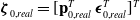 ${\boldsymbol{\mathbf{\zeta }}}_{0,real}=[{\boldsymbol{\mathbf{p}}}_{0,real}^T \; {\boldsymbol{\mathbf{\epsilon }}}_{0,real}^T]^T$
and use it as ground truth for the self-calibration results, a manual homing procedure was performed before each test. The platform was positioned against a mechanical support where the nominal values of cable lengths, swivel angles, and yaw were previously measured with a high-precision photogrammetry system.
${\boldsymbol{\mathbf{\zeta }}}_{0,real}=[{\boldsymbol{\mathbf{p}}}_{0,real}^T \; {\boldsymbol{\mathbf{\epsilon }}}_{0,real}^T]^T$
and use it as ground truth for the self-calibration results, a manual homing procedure was performed before each test. The platform was positioned against a mechanical support where the nominal values of cable lengths, swivel angles, and yaw were previously measured with a high-precision photogrammetry system.
Extperimental setup.

Geometrical parameters of the 4-cable UACDPR prototype.

After the static workspace analysis, the translational bounds were set as:
 \begin{equation} {\boldsymbol{\mathbf{p}}}_{lb} = \begin{bmatrix}-0.4&\quad-0.4&\quad0.6\end{bmatrix}^T \;\mathrm{m} \quad \mathrm{and} \quad {\boldsymbol{\mathbf{p}}}_{ub}=\begin{bmatrix}0.4&\quad0.4&\quad1.2\end{bmatrix}^T \; \mathrm{m}. \end{equation}
The choice of the number of measurement poses
 $k$
was guided by the main objective of this work: achieving automatic self-calibration in reduced time, without compromising accuracy. For the same reason, our evaluation is mainly based on the calibration time. To analyze the effect of different measurement-pose sets on the initial-pose self-calibration, two spatial grids were discretized using different values of
$k$
was guided by the main objective of this work: achieving automatic self-calibration in reduced time, without compromising accuracy. For the same reason, our evaluation is mainly based on the calibration time. To analyze the effect of different measurement-pose sets on the initial-pose self-calibration, two spatial grids were discretized using different values of
 $n_x$
,
$n_x$
,
 $n_y$
, and
$n_y$
, and
 $n_z$
. In the first grid,
$n_z$
. In the first grid,
 $n_x = n_y = n_z = 2$
, resulting in a total of
$n_x = n_y = n_z = 2$
, resulting in a total of
 $k = 8$
equilibrium poses. In the second grid,
$k = 8$
equilibrium poses. In the second grid,
 $n_x = n_y = n_z = 3$
, yielding
$n_x = n_y = n_z = 3$
, yielding
 $k = 27$
poses. The equilibrium poses
$k = 27$
poses. The equilibrium poses
 ${\boldsymbol{\mathbf{Z}}}_{ideal}$
and tension setpoints
${\boldsymbol{\mathbf{Z}}}_{ideal}$
and tension setpoints
 ${\boldsymbol{\mathbf{T}}}_{setpoint}$
for
${\boldsymbol{\mathbf{T}}}_{setpoint}$
for
 $k=2$
are reported in Table II as an example, while results for
$k=2$
are reported in Table II as an example, while results for
 $k=27$
are omitted as they do not provide additional insights.
$k=27$
are omitted as they do not provide additional insights.
The initial tension setpoint was set close to the first component
 ${\boldsymbol{\mathbf{\tau }}}_1$
of
${\boldsymbol{\mathbf{\tau }}}_1$
of
 ${\boldsymbol{\mathbf{T}}}_{setpoint}$
(which is the same for the two grids), at
${\boldsymbol{\mathbf{T}}}_{setpoint}$
(which is the same for the two grids), at
 ${\boldsymbol{\mathbf{\tau }}}_0=[100.00\; 100.00\; 100.00\; 100.00]$
N. The data logging rate for all sensors was 100 ms, balancing file size and data resolution. The self-calibration problem (14) was solved using a PC with a 13th generation Intel i7 processor and 32 GB of RAM, distributing the computation across 14 cores. For both
${\boldsymbol{\mathbf{\tau }}}_0=[100.00\; 100.00\; 100.00\; 100.00]$
N. The data logging rate for all sensors was 100 ms, balancing file size and data resolution. The self-calibration problem (14) was solved using a PC with a 13th generation Intel i7 processor and 32 GB of RAM, distributing the computation across 14 cores. For both
 $j=\tau l\sigma \epsilon$
and
$j=\tau l\sigma \epsilon$
and
 $j=l\sigma \epsilon$
the fmincon MATLAB routine with a trust-region-reflective algorithm was used with a termination tolerance of
$j=l\sigma \epsilon$
the fmincon MATLAB routine with a trust-region-reflective algorithm was used with a termination tolerance of
 $10^{-10}$
on the function value, of
$10^{-10}$
on the function value, of
 $10^{-8}$
on the first-order optimality, and of
$10^{-8}$
on the first-order optimality, and of
 $10^{-10}$
on the optimization variables. The gradient was analytically formulated to improve computational efficiency, as in [Reference Zoffoli, Ida’, Carricato, Quaglia, Boschetti and Carbone23], and the initial guess was generated using the methods described in Section 3.3. A graphical representation of the measured tensions, along with the reference trajectory
$10^{-10}$
on the optimization variables. The gradient was analytically formulated to improve computational efficiency, as in [Reference Zoffoli, Ida’, Carricato, Quaglia, Boschetti and Carbone23], and the initial guess was generated using the methods described in Section 3.3. A graphical representation of the measured tensions, along with the reference trajectory
 $\hat {{\boldsymbol{\mathbf{\tau }}}}$
used to transition between the equilibrium configurations, is shown in Figure 5.
$\hat {{\boldsymbol{\mathbf{\tau }}}}$
used to transition between the equilibrium configurations, is shown in Figure 5.
Ideal measurement poses and tension setpoints, with
 $n_x=n_y=n_z=2$
.
$n_x=n_y=n_z=2$
.

Sampled and reference tensions with
 $k$
= 8. The black curves, with superscript
$k$
= 8. The black curves, with superscript
 $(\:\hat {}\:)$
, represent the tension reference applied during transitions, while the colored curves are the measured tensions, with superscript
$(\:\hat {}\:)$
, represent the tension reference applied during transitions, while the colored curves are the measured tensions, with superscript
 $(\:^*\:)$
.
$(\:^*\:)$
.

The results of the two self-calibration methods introduced in Section 3.1 are reported in Table III, where the following data are specified:
-
• the used sensor set
$j$
, and thus, the related self-calibration algorithm; -
• the total self-calibration time
$t_{sc}$
, composed by the data acquisition time and initial-pose estimation time; -
• the number of pose measurements
$k$
used in the algorithm; -
• the resulting initial position error norm
$\varepsilon _p=\|{\boldsymbol{\mathbf{p}}}_{0,real}-{\boldsymbol{\mathbf{p}}}_{0,sol}\|$
; -
• the resulting initial orientation error
$\varepsilon _{r}=|\alpha _{0,real}-\alpha _{0,sol}|$
, where
$\alpha _0$
is the rotation angle in the axis-angle parameterization of the initial orientation. The angle
$\alpha$
is obtained from the rotation matrix
${\boldsymbol{\mathbf{R}}}({\boldsymbol{\mathbf{\epsilon }}})$
as:(20)
\begin{equation} \alpha = \arccos \left (\frac {{\boldsymbol{\mathbf{R}}}_{1,1}(\epsilon )+{\boldsymbol{\mathbf{R}}}_{2,2}(\epsilon )+{\boldsymbol{\mathbf{R}}}_{3,3}(\epsilon )-1}{2}\right ). \end{equation}


Trials
 $a$
and
$a$
and
 $b$
share the same dataset, corresponding to the data acquisition in which the EE transitioned between 8 equilibrium poses. Similarly, trials
$b$
share the same dataset, corresponding to the data acquisition in which the EE transitioned between 8 equilibrium poses. Similarly, trials
 $c$
and
$c$
and
 $d$
share a dataset where the EE followed the path with 27 equilibrium poses. Therefore, the data acquisition time for trials
$d$
share a dataset where the EE followed the path with 27 equilibrium poses. Therefore, the data acquisition time for trials
 $a$
and
$a$
and
 $b$
is the same and equal to
$b$
is the same and equal to
 $t_{da} = 2.13$
min, whereas
$t_{da} = 2.13$
min, whereas
 $t_{da}=5.11$
min for trials
$t_{da}=5.11$
min for trials
 $c$
and
$c$
and
 $d$
. The total self-calibration time
$d$
. The total self-calibration time
 $t_{sc}$
reported in Table III consists of both the data acquisition time
$t_{sc}$
reported in Table III consists of both the data acquisition time
 $t_{da}$
and the computational time required by the solver
$t_{da}$
and the computational time required by the solver
 $t_{opt}$
, which depends on the number of poses
$t_{opt}$
, which depends on the number of poses
 $k$
used in the optimization. For trials
$k$
used in the optimization. For trials
 $b$
and
$b$
and
 $d$
, where cable tension measurements were not used, the pose sampling rate from the logged dataset was chosen such that the number of extracted poses
$d$
, where cable tension measurements were not used, the pose sampling rate from the logged dataset was chosen such that the number of extracted poses
 $k$
yielded an optimization time
$k$
yielded an optimization time
 $t_{opt}$
approximately equal to that of their tension-based counterparts (trials
$t_{opt}$
approximately equal to that of their tension-based counterparts (trials
 $a$
and
$a$
and
 $c$
). This ensured a fair comparison between methods that do and do not utilize load-cell measurements.
$c$
). This ensured a fair comparison between methods that do and do not utilize load-cell measurements.
Initial-pose self-calibration algorithm results.

Incorporating tension measurements (
 $j=\tau l\sigma \epsilon$
) substantially improves position accuracy. For instance, using only 8 equilibrium poses, the error drops from 23 mm (trial
$j=\tau l\sigma \epsilon$
) substantially improves position accuracy. For instance, using only 8 equilibrium poses, the error drops from 23 mm (trial
 $b$
) to 12 mm (trial
$b$
) to 12 mm (trial
 $a$
). Similarly, for
$a$
). Similarly, for
 $k=27$
, it decreases from 22 mm (trial
$k=27$
, it decreases from 22 mm (trial
 $d$
) to 7.2 mm (trial
$d$
) to 7.2 mm (trial
 $c$
). This trend confirms that static equilibrium constraints and cable tension measurements significantly enhance positional accuracy. The effect on orientation accuracy is more difficult to interpret. When comparing trials
$c$
). This trend confirms that static equilibrium constraints and cable tension measurements significantly enhance positional accuracy. The effect on orientation accuracy is more difficult to interpret. When comparing trials
 $a$
and
$a$
and
 $b$
, the inclusion of tension measurements reduces the orientation error from
$b$
, the inclusion of tension measurements reduces the orientation error from
 $5.44^\circ$
to
$5.44^\circ$
to
 $1.24^\circ$
, showing a clear benefit. However, this trend does not persist when increasing the number of poses. In fact, trial
$1.24^\circ$
, showing a clear benefit. However, this trend does not persist when increasing the number of poses. In fact, trial
 $c$
(tension-based) results in a worse orientation estimate (
$c$
(tension-based) results in a worse orientation estimate (
 $3.14^\circ$
) than trial
$3.14^\circ$
) than trial
 $a$
(
$a$
(
 $1.24^\circ$
). This may be due to less favorable pose distribution or greater noise influence in the larger dataset. Conversely, in the kinematic-only approach, increasing
$1.24^\circ$
). This may be due to less favorable pose distribution or greater noise influence in the larger dataset. Conversely, in the kinematic-only approach, increasing
 $k$
from 19 (trial
$k$
from 19 (trial
 $b$
) to 128 (trial
$b$
) to 128 (trial
 $d$
) halves the orientation error (
$d$
) halves the orientation error (
 $5.44^\circ$
to
$5.44^\circ$
to
 $2.86^\circ$
), as expected. These results suggest that the impact of the number of measurement poses on orientation accuracy is method-dependent: while the kinematic-only method benefits from more poses, the tension-based method does not exhibit a clear trend and may be sensitive to dataset-specific factors.
$2.86^\circ$
), as expected. These results suggest that the impact of the number of measurement poses on orientation accuracy is method-dependent: while the kinematic-only method benefits from more poses, the tension-based method does not exhibit a clear trend and may be sensitive to dataset-specific factors.
Overall, the tension-based method (
 $a$
,
$a$
,
 $c$
) achieves better position accuracy while requiring significantly fewer measurements than the kinematic-only method (
$c$
) achieves better position accuracy while requiring significantly fewer measurements than the kinematic-only method (
 $b$
,
$b$
,
 $d$
). This is particularly noteworthy because the tension-based method relies on a simplified physical model (neglecting cable sag and elasticity) and uses cable-tension measurements, which typically carry greater uncertainty than kinematic signals. Yet, despite these limitations, the inclusion of tension data and equilibrium constraints consistently improves the positional estimate. It is also important to note that, although internal statics has been previously used in self-calibration problems [Reference Idá, Merlet, Carricato, Pott and Bruckmann14], to our knowledge, direct use of cable tension measurements for initial-pose self-calibration in UACDPRs is novel. This work therefore provides the first quantitative comparison of statics- vs. kinematics-based methods using real tension data. To obtain self-calibration results comparable to those reported in [Reference Zoffoli, Ida’, Carricato, Quaglia, Boschetti and Carbone23], which achieved a best-case accuracy of
$d$
). This is particularly noteworthy because the tension-based method relies on a simplified physical model (neglecting cable sag and elasticity) and uses cable-tension measurements, which typically carry greater uncertainty than kinematic signals. Yet, despite these limitations, the inclusion of tension data and equilibrium constraints consistently improves the positional estimate. It is also important to note that, although internal statics has been previously used in self-calibration problems [Reference Idá, Merlet, Carricato, Pott and Bruckmann14], to our knowledge, direct use of cable tension measurements for initial-pose self-calibration in UACDPRs is novel. This work therefore provides the first quantitative comparison of statics- vs. kinematics-based methods using real tension data. To obtain self-calibration results comparable to those reported in [Reference Zoffoli, Ida’, Carricato, Quaglia, Boschetti and Carbone23], which achieved a best-case accuracy of
 $\varepsilon _p = 23.36$
mm and
$\varepsilon _p = 23.36$
mm and
 $\varepsilon _r = 2.18^\circ$
using a fast but manual procedure, the kinematic-only approach requires at least
$\varepsilon _r = 2.18^\circ$
using a fast but manual procedure, the kinematic-only approach requires at least
 $k=128$
poses and a total calibration time of over 10 minutes. In contrast, the tension-based method achieves better performance with just
$k=128$
poses and a total calibration time of over 10 minutes. In contrast, the tension-based method achieves better performance with just
 $k=8$
and with the same self-calibration duration. These findings emphasize the importance of exploiting static configurations and cable-tension measurements to enable fast and accurate automatic self-calibration in UACDPRs.
$k=8$
and with the same self-calibration duration. These findings emphasize the importance of exploiting static configurations and cable-tension measurements to enable fast and accurate automatic self-calibration in UACDPRs.
5. Conclusions
In this paper, we presented a novel data acquisition framework for initial-pose self-calibration in UACDPRs. The proposed procedures support automatic and rapid data collection, extending the approach introduced in [Reference Zoffoli, Ida’, Carricato, Quaglia, Boschetti and Carbone23], which was fast but not automated. We improve upon [Reference Idá, Merlet, Carricato, Pott and Bruckmann14], where high accuracy required prolonged acquisition durations.
The proposed approach exploits pure force joint control to guide the EE through static equilibrium configurations while ensuring that cable constraints remain active. By incorporating multiple sensor measurements, including cable tensions, into the calibration process, the number of required measurement poses is significantly reduced while maintaining high accuracy in the initial-pose estimation. An experimental validation demonstrated that using static equilibrium poses in the calibration problem is mandatory to obtain accurate results in the estimation of the initial position. In particular, our analysis demonstrated that leveraging force measurements effectively reduces the number of required configurations, thus minimizing calibration time.
For future work, we aim to further automate the data acquisition process by developing a comprehensive tool that integrates automatic measurement pose selection, motion planning, and a control strategy to minimize both the path length and transition time between equilibrium poses, thus reducing unnecessary motion and overall data acquisition time. Another objective is to eliminate the need for an initial trajectory tuning phase, which currently must be repeated after each reconfiguration of the UACDPR and limits the system’s full automation potential. Additionally, we plan to integrate the two self-calibration methods presented in this paper into a unified approach, leveraging their respective advantages: achieving high accuracy in both initial position and orientation while minimizing the required number of equilibrium poses. A key challenge in this integration will be designing an algorithm for automatic data extraction from logged measurements, ensuring that static equations are applied only when the EE is in equilibrium configurations, while other sampled data contributes to the kinematic formulation.
Author contributions
F. Zoffoli and E. Idà conceived and designed the study. F. Zoffoli conducted data gathering and data processing. M. Carricato provided funding for the study and experimentation. F. Zoffoli, E. Idà, and M. Carricato wrote the article.
Financial support
This study was carried out within the MICS (Made in Italy - Circular and Sustainable) Extended Partnership and received funding from the European Union Next-GenerationEU (PIANO NAZIONALE DI RIPRESA E RESILIENZA (PNRR) - MISSIONE 4 COMPONENTE 2, INVESTIMENTO 1.3 - D.D. 1551.11-10-2022, PE00000004), and thanks to the support of the Italian Ministry of University and Research (MUR) through the PRIN 2020 grant “Extending Robotic Manipulation Capabilities by Cooperative Mobile and Flexible Multi-Robot Systems (Co-MiR)” (No. 2020CMEFPK).
Competing interests
The authors declare no conflicts of interest exist.
Data availability
The complete dataset used in this study has been made publicly available in [Reference Ida’40].
Ethical approval
Not applicable.
A. Static workspace evaluation
Following the approach described in [Reference Ida’ and Carricato8], the modified inverse geometrico-static problem consists of determining the cable tensions and the EE orientation for a given EE position within the workspace, under a fixed tension distribution strategy (such as the barycentric method [Reference Lamaury, Gouttefarde, Bruckmann and Pott39]). This leads to solving, at each point, a system of three nonlinear equations in three unknowns (namely the EE orientation):
 \begin{equation} (\boldsymbol{\mathbf{\Xi }}^T_M\boldsymbol{\mathbf{\Xi }}^{-T}_F-\tilde {\boldsymbol{\mathbf{s}}}')\boldsymbol{\mathbf{g}}+\boldsymbol{\mathbf{\Xi }}^T_M\boldsymbol{\mathbf{\Xi }}^{-T\perp }_F\boldsymbol{\mathbf{\lambda }} = \boldsymbol{\mathbf{0}}_{3\times 1} \end{equation}
where
-
•
$\boldsymbol{\mathbf{\Xi }}_F^{T}\in \mathbb{R}^{3\times n}$
and
$\boldsymbol{\mathbf{\Xi }}_M^{T}\in \mathbb{R}^{3\times n}$
are the translational and rotational blocks of the structure matrix
$\boldsymbol{\mathbf{\Xi }}_l^T$
; -
•
$\boldsymbol{\mathbf{\Xi }}^{-T}_F\in \mathbb{R}^{n\times 3}$
is any right inverse of
$\boldsymbol{\mathbf{\Xi }}^{T}_F$
and
$\boldsymbol{\mathbf{\Xi }}^{T\perp }_F\in \mathbb{R}^{m\times (n-3)}$
spans the nullspace of
$\boldsymbol{\mathbf{\Xi }}^{T}_F$
; -
•
$\boldsymbol{\lambda }\in \mathbb{R}^{(n-3)\times 1}$
is the array derived by the chosen tension distribution algorithm.


Then, cable tensions are obtained as:
 \begin{equation} \boldsymbol{\mathbf{\tau }} = \boldsymbol{\mathbf{\Xi }}^{-T}_F\boldsymbol{\mathbf{g}} + \boldsymbol{\mathbf{\Xi }}^{T\perp }_F\boldsymbol{\mathbf{\lambda }}. \end{equation}
If the tensions satisfy the inequality constraints
 \begin{equation} \tau _{min} \preceq \boldsymbol{\mathbf{\tau }} \preceq \tau _{max} \end{equation}
and the pose is statically stable, then the pose is included in the static workspace. Static stability is assessed by verifying the positiveness of the free-motion stiffness matrix
 $\boldsymbol{\mathbf{K}}^\perp _f$
[Reference Idà, Briot and Carricato25]:
$\boldsymbol{\mathbf{K}}^\perp _f$
[Reference Idà, Briot and Carricato25]:
 \begin{equation} \boldsymbol{\mathbf{K}}_f^\perp \triangleq {\boldsymbol{\mathbf{\Xi }}}^{\perp T}({\boldsymbol{\mathbf{K}}} +{\boldsymbol{\mathbf{Q}}}){\boldsymbol{\mathbf{\Xi }}}^\perp \end{equation}
where
 ${\boldsymbol{\mathbf{\Xi }}}^{\perp T}\in \mathbf{R}^{(6-n)\times 6}$
is any left nullspace basis of
${\boldsymbol{\mathbf{\Xi }}}^{\perp T}\in \mathbf{R}^{(6-n)\times 6}$
is any left nullspace basis of
 ${\boldsymbol{\mathbf{\Xi }}}^{T}$
(
${\boldsymbol{\mathbf{\Xi }}}^{T}$
(
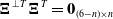 ${\boldsymbol{\mathbf{\Xi }}}^{\perp T}{\boldsymbol{\mathbf{\Xi }}}^{T}={\boldsymbol{\mathbf{0}}}_{(6-n)\times n}$
) and the matrices
${\boldsymbol{\mathbf{\Xi }}}^{\perp T}{\boldsymbol{\mathbf{\Xi }}}^{T}={\boldsymbol{\mathbf{0}}}_{(6-n)\times n}$
) and the matrices
 $\boldsymbol{\mathbf{K}}$
and
$\boldsymbol{\mathbf{K}}$
and
 $\boldsymbol{\mathbf{Q}}$
are defined as:
$\boldsymbol{\mathbf{Q}}$
are defined as:
 \begin{equation} \begin{split} {\boldsymbol{\mathbf{K}}} &\triangleq \sum _{i=1}^n \tau _i \left[\begin{array}{c@{\quad}c} {\boldsymbol{\mathbf{T}}}_i & -{\boldsymbol{\mathbf{T}}}_i\tilde {{\boldsymbol{\mathbf{a}}}}_i' \\ \tilde {{\boldsymbol{\mathbf{a}}}}'_i{\boldsymbol{\mathbf{T}}}_i & -\tilde {{\boldsymbol{\mathbf{a}}}}_i'{\boldsymbol{\mathbf{T}}}\tilde {{\boldsymbol{\mathbf{a}}}}_i' \end{array}\right] + \sum _{i=1}^n \tau _i \left[\begin{array}{c@{\quad}c} {\boldsymbol{\mathbf{0}}}_{3\times 3} & {\boldsymbol{\mathbf{0}}}_{3\times 3} \\ {\boldsymbol{\mathbf{0}}}_{3\times 3} & \tilde {{\boldsymbol{\mathbf{t}}}}_i\tilde {{\boldsymbol{\mathbf{a}}}}_i' \end{array}\right], \\[6pt] {\boldsymbol{\mathbf{T}}}_i &\triangleq \frac {\|{\boldsymbol{\mathbf{u}}}_i\times {\boldsymbol{\mathbf{n}}}_i\|{\boldsymbol{\mathbf{w}}}_i{\boldsymbol{\mathbf{w}}}_i^T}{{\boldsymbol{\mathbf{u}}}_i\cdot ({\boldsymbol{\mathbf{a}}}_i-{\boldsymbol{\mathbf{d}}}_i)} + \frac {{\boldsymbol{\mathbf{n}}}_i{\boldsymbol{\mathbf{n}}}_i^T}{\|\boldsymbol{\mathbf{\rho }}_i\|}, \qquad {\boldsymbol{\mathbf{Q}}}\triangleq \left[\begin{array}{c@{\quad}c} {\boldsymbol{\mathbf{0}}}_{3\times 3} & {\boldsymbol{\mathbf{0}}}_{3\times 3} \\ {\boldsymbol{\mathbf{0}}}_{3\times 3} & \tilde {{\boldsymbol{\mathbf{s}}}}'\tilde {{\boldsymbol{\mathbf{g}}}} \end{array}\right]. \end{split} \end{equation}


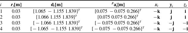
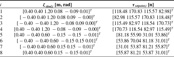


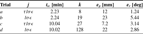

 Open access