


Introduction
Pesticide movement from intended targets onto unintended targets has been a concern as long as pesticides have been applied. The first report recognizing pesticides as air pollutants occurred in 1946 (Daines Reference Daines and McCabe1952). In 1953, authors of a Stanford Law Review article summarized the conflict of pesticide drift well: “Science has created weapons which are of inestimable value to many farmers, but which threaten the economic existence of others.” (Stanford Law Review 1953).
Commercial introduction of crops with dicamba-resistant traits and subsequent off-target movement of dicamba herbicide is the most recent example of large-scale pesticide movement. However, pesticides moving off target in large quantities is not a novel concern, and additional examples, including those outlined below, have advanced our understanding and guided research on aerial pesticide movement.
Introduction of 2,4-D and Crop Dusting
The U.S. agriculture industry rapidly adopted the practice of applying pesticides via crop dusting in the early 1950s. Commercial introduction of 2,4-D; the return of newly unemployed, World War II-trained military pilots; and a surplus of military planes provided the opportunities for this expansion (Stanford Law Review 1953). It was common for crop dusters to apply pesticides in the early morning or after sundown to avoid physical drift associated with higher midday wind speeds (Stanford Law Review 1953). This practice likely resulted in pesticides being applied during inversion-like conditions. The increase in crop dusting applications resulted in an increase in legal pesticide drift cases, and in 1952–1953, nine crop dusting cases reached the appellate court (Akesson and Yates Reference Akesson and Yates1964; Stanford Law Review 1953).
The Grape-Growing Region of the Yakima Valley
Large-scale off-target movement of 2,4-D continued to be a problem into the next decades. The wheat and grape-growing regions of Yakima Valley in Washington state occur in close proximity, and by the 1960s, herbicide damage in the grape-growing region, resulting from applications of 2,4-D to wheat, was severe and widespread. Air sampling research conducted in the Yakima Valley region in the early 1970s indicated that 2,4-D had traveled approximately 16 km from wheat fields to vineyards and in sufficient quantities to injure grapes (Reisenger and Robinson Reference Reisner and Robinson1976). It was during these observations that the term “air mass” damage was derived (Robinson and Fox Reference Robinson and Fox1978). “Air mass” damage referred to large areas where consistent herbicide injury symptoms appeared on the sensitive crop without a definable gradient and was speculated to be the result of a large, contaminated cloud passing through the area (Robinson and Fox Reference Robinson and Fox1978). The state began banning highly volatile 2,4-D formulations and enforcing cutoff dates in specific counties in the early 1970s (Reisenger and Robinson Reference Reisner and Robinson1976; Robinson and Fox Reference Robinson and Fox1978).
Dichlorodiphenyltrichloroethane in the Atmosphere
Off-target movement of the highly persistent insecticide organochlorine dichlorodiphenyltrichloroethane (DDT) resulted in several research studies conducted in the 1980s. Results from air sampling research conducted aboard ships in the Arabian Sea, Indian Ocean, and north Atlantic Ocean indicated that DDT was 25 to 40 times more highly concentrated over waters in proximity to regions where the chemical was still used compared with areas where the chemical had been banned (Bidleman and Leonard Reference Bidleman and Leonard1982). Findings from Bidleman and Leonard’s study combined with other research reviewed by Pimentel and Levitan (Reference Pimentel and Levitan1986) led to the conclusion that atmospheric pesticide levels are a function of the location where application occurred, wind direction at application, subsequent movement of air masses containing pesticides, and atmospheric transport time.
Postemergence Dicamba Applications to Soybean and Cotton
The most recent off-target dicamba injury observations (Bish et al. Reference Bish, Guinan and Bradley2019b; Bradley Reference Bradley2017a, Reference Bradley2017b; Steckel Reference Steckel2017) were unique in that applications could only be made by via ground sprayers. However, reported damage was still extensive (Figure 1) (Bish et al. Reference Bish, Guinan and Bradley2019b; Bradley Reference Bradley2017b; Steckel Reference Steckel2017). In 2017, off-target movement of dicamba resulted in 2,708 dicamba-related injury investigations by state departments of agriculture (Figure 1; Oseland et al. Reference Oseland, Bish, Steckel and Bradley2020). During this same year, state extension weed scientists estimated that approximately 1.5 million ha of soybean were reported to be injured by dicamba in the United States (Bradley Reference Bradley2017b). Additional reports of injury to sensitive, nontarget vegetation were extensively documented throughout 2018, 2019, and 2020, especially in areas where adoption of soybean and cotton crops with the dicamba-resistant trait was highest (Bradley Reference Bradley2018; Hager Reference Hager2019; Hartzler Reference Hartzler2020a; Hartzler Reference Hartzler2020b; Johnson and Ikley Reference Johnson and Ikley2018; Steckel Reference Steckel2018, Reference Steckel2019; Zimmer et al. Reference Zimmer, Hayden, Whitford, Young and Johnson2019; Zimmer and Johnson Reference Zimmer and Johnson2020). In a recent survey of state departments of agriculture posted on the Association of American Pesticide Control Officials (AAPCO) website, 151 dicamba-related cases were reported in Illinois, 116 in Minnesota, 102 in Missouri, 73 in Indiana, and 63 in Nebraska (AAPCO 2020). At least two surveys, including the AAPCO survey, noted that underreporting of dicamba injury to state departments of agriculture is common (AAPCO 2020; Bradley Reference Bradley2019). Based on these numbers and observations, it seems that the extent of off-target movement of dicamba that has occurred during this time period is more substantial than any chemical movement previously experienced in U.S. agricultural history.

Figure 1. Number of dicamba-related injury claims reported by state departments of agriculture in 2017, which was the first year dicamba could legally be applied over the top of dicamba-resistant soybean and cotton.
Once off-target movement of dicamba began to appear in areas where adoption of crops with the dicamba-resistance traits was higher (i.e., southeastern Missouri, northeastern Arkansas, and western Tennessee), one observation that became immediately apparent was the extent of injury that occurred across entire fields of dicamba-sensitive soybean (Bradley Reference Bradley2017a; Hager Reference Hager2017; Loux and Johnson Reference Loux and Johnson2017; Steckel Reference Steckel2017). Extension weed scientists and others who became involved in visiting these injured fields commonly reported a phenomenon in which essentially no discernable differences in the severity of the dicamba injury could be observed across entire fields of dicamba-sensitive soybean, regardless of the size of the injured field or proximity to the source of the suspected off-target movement. This phenomenon came to be known as the “landscape-level effect” and can likely be attributed to a combination of factors including 1) the extreme sensitivity of non-dicamba–resistant soybean to even the most minute quantities of dicamba (Hartzler Reference Hartzler2020b; Solomon and Bradley Reference Solomon and Bradley2014); 2) innate sensitivity of many other broadleaf species to dicamba (summarized in Table 1); and 3) the tendency of ground-based applications of dicamba to move into and within the atmosphere through factors that influence secondary movement.
Table 1. Select literature on sensitivity of species to dicamba and/or 2,4-D arranged by year published from oldest to newest.

Primary and Secondary Pesticide Movement
Pesticide drift is commonly described as either primary or secondary movement. Primary movement occurs when pesticides move off target at the time of application (Carlsen et al. Reference Carlsen, Spliid and Svensmark2006; Jones et al. Reference Jones, Norsworthy and Barber2019). The terms primary movement, primary drift, spray drift, and direct drift are often used interchangeably (Carlsen et al. Reference Carlsen, Spliid and Svensmark2006). This drift is the result of an active ingredient of a pesticide being transported away from the intended area after coming through the application spray nozzle, due to air flow at the time of application (Combellack Reference Combellack1982). Primary drift is not affected by the formulation of a pesticide’s active ingredient (Bird et al. Reference Bird, Esterly and Perry1996; Carlsen et al. Reference Carlsen, Spliid and Svensmark2006). Many factors that result in primary movement are largely within an applicator’s control (Bish and Bradley Reference Bish and Bradley2017; Vangessel and Johnson Reference Vangessel and Johnson2005). The scope of this review does not include analysis of these factors, which include nozzle type, droplet size, adjuvants, boom height, and sprayer speed.
Secondary movement occurs after herbicide application (Jones et al. Reference Jones, Norsworthy and Barber2019; Mueller Reference Mueller2015). Variables that affect secondary movement are much more difficult to control than those associated with primary movement and can be more difficult to characterize. Vapor drift is one form of secondary movement and is the result of chemicals volatilizing into the atmosphere. Wind erosion is another form and occurs when the pesticide is deposited on the intended surface but is moved back into the atmosphere with the soil particulate to which it is bound (Clay et al. Reference Clay, DeSutter and Clay2001). Application method, size and chemical makeup of soil particulate, and herbicide dissipation rates affect secondary movement by wind erosion. In a comparison of residual herbicides incorporated into the soil and herbicides applied on undisturbed soils, the amount of herbicide collected on wind-erodible soil sediments was approximately 8% and 65%, respectively (Clay et al. Reference Clay, DeSutter and Clay2001). Additionally, pesticides applied during stable atmospheric conditions can remain in the atmosphere and be readily available for secondary movement (Bish et al. Reference Bish, Farrell, Lerch and Bradley2019a). Although these conditions might seem like the perfect time to spray to minimize physical drift, they can result in high levels of off-target pesticide movement (Bird et al. Reference Bird, Esterly and Perry1996).
This review covers our current understanding of how pesticides move into or remain in the atmosphere and become available for secondary movement. Much of the review will encompass research specific to dicamba and 2,4-D. The extreme sensitivity of nonresistant plants, distinct injury symptoms, and historical volatility issues associated with these chemicals have resulted in a vast array of studies published in the literature. However, most of the factors discussed in this review will apply to pesticide movement in general.
Factors That Promote Volatility
Volatility allows chemicals to return to the atmosphere and become available for off-target transport. Synthetic auxin herbicides such as 2,4-D and dicamba are prone to volatility due to their chemical properties. A study conducted in Canada in the late 1970s suggested that vapor drift was the major contributor to off-target 2,4-D movement with an estimated 35% of high-volatile 2,4-D formulations volatilizing off of Canadian prairie soils (Maybank et al. Reference Maybank, Yoshida and Grover1978). Later in the 1970s, Behrens and Lueschen (Reference Behrens and Lueschen1979) found that dicamba applied to corn could volatilize in sufficient quantities to injure soybean for up to 3 d following application and cause symptoms to sensitive soybean plants 60 m from the treated area. They also found that of four formulations tested, the acid form of dicamba was most susceptible to volatilize in laboratory settings, and that dicamba volatilized more readily from soybean and corn leaf surfaces than from soil (Behrens and Lueschen Reference Behrens and Lueschen1979).
The vapor pressure of synthetic auxin herbicides is in general higher relative to many other common herbicides, and subtle increases in air temperature can result in more rapid transition of molecules from liquid to vapor (Spencer and Cliath Reference Spencer and Cliath1983). New 2,4-D and dicamba formulations have since been developed to reduce volatility in large part by reducing the vapor pressure of the chemical. Two of the most recently developed formulations of dicamba salts, the diglycolamine salt of dicamba combined with an acetic acid:acetate pH modifier (DGA-VG) and the N,N-bis-(3-aminopropyl)methylamine salt of dicamba (BAPMA), have much lower vapor pressures than dicamba acid (Hartzler Reference Hartzler2017; Hemminghaus et al. Reference Hemminghaus, MacInnes and Zhang2017; MacInnes Reference MacInnes2017; Werle et al. Reference Werle, Oliverira, Jhala, Procotor, Rees and Klein2018). However, both formulations were detected for 72 h after application in air sampling studies conducted 20 cm above the soybean canopy indicating that detectable amounts of these new formulations were volatilizing over time (Bish et al. Reference Bish, Farrell, Lerch and Bradley2019a). Using bioassay plants, Jones et al (Reference Jones, Norsworthy, Barber, Gbur and Krueger2018) showed that injury associated with secondary movement, indicative of volatility of BAPMA and DGA-VG applications, could be observed at 108 m and 180 m from the sites of application, respectively (Jones et al. Reference Jones, Norsworthy, Barber, Gbur and Krueger2018). These results provide more research support to field observations that lower-volatile dicamba formulations can volatilize in meaningful quantities.
Research on the most recent formulation of 2,4-D known as 2,4-D choline, the choline being a quaternary ammonium salt, has shown reduced volatility when tested in Georgia using cotton as bioassay plants (Sosnoskie et al. Reference Sosnoskie, Culpepper, Braxton and Richbrug2015). Potted cotton plants were placed outside of treated plots approximately 1 h after applications with three formulations of 2,4-D and removed at either 24 h or 48 h following application. Injury from the 2,4-D choline application was not detected further than 1.5 m from the site of application. Older formulations of 2,4-D ester and 2,4-D amine moved 48 m and 3 m from the treated sites, respectively (Sosnoskie et al. Reference Sosnoskie, Culpepper, Braxton and Richbrug2015). It is important to note that a complete understanding of 2,4-D choline volatility and secondary movement may not occur until 2,4-D resistant cotton and soybean are grown on a larger scale for concurrent years.
Additional factors that can influence volatility include a plant’s ability to absorb the chemical, pH of the environment, and air temperature. The rate of chemical uptake affects how long the pesticide is available on the surface for volatilization. Uptake is influenced by epicuticle thickness of the leaf on which the droplet lands (Baker and Hunt Reference Baker and Hunt1981) and relative humidity at the surface of the leaf, which influences stomatal conductance (Pallas Reference Pallas1960). Legleiter et al. (Reference Legleiter, Young and Johnson2018) found that following applications of 2,4-D plus glyphosate with various nozzles and over four weed species, 2,4-D levels on the leaf surfaces were 4% to 16.6% of the initial levels at 24 h after application. Studies in the early 1970s showed that 40% of radiolabeled dicamba applied to wheat or Tartary buckwheat leaves remained on the leaves after 24 h (Chang and Vanden Born Reference Chang and Vanden Born1971). In 1993, research showed that surface residues of 2,4-D and dicamba on wheat plants was greatly reduced 24 h after application (Cessna Reference Cessna1993). We have preliminary data indicating that DGA-VG can be detected on soybean leaf surfaces 48 h after an application; however, we are unaware of any peer-reviewed literature on the half-lives of new dicamba formulations on leaf surfaces.
Dicamba is most likely to convert to the highly volatile dicamba acid as pH lowers to near 5 (Abraham Reference Abraham2018). Sources that can influence dicamba pH include spray tank solution pH and soil pH (Mueller and Steckel Reference Mueller and Steckel2019a; Oseland et al. Reference Oseland, Bish, Steckel and Bradley2020). Other sources such as pH of morning dew on leaf surfaces are also likely. Mueller and Steckel found that adding glyphosate to the DGA-VG or BAPMA formulations of dicamba decreased spray tank formulation to a pH of near or below 5.0 depending on the carrier volume and starting pH of the water source (Mueller and Steckel Reference Mueller and Steckel2019a). They went on to show that addition of glyphosate to DGA-VG increased the amount of dicamba detected compared with dicamba alone (Mueller and Steckel Reference Mueller and Steckel2019b). Those findings were similar to ours, in which addition of glyphosate to a dicamba spray solution increased the amount of dicamba detected in the air from 4.45 ng m−3 to 8.45 ng m−3 (Bish et al. Reference Bish, Farrell, Lerch and Bradley2019a). More recently, we found that soil pH can affect the likelihood of dicamba volatilization (Oseland et al. Reference Oseland, Bish, Steckel and Bradley2020). In a series of binary logistic regression models developed to identify weather and environmental factors that improve the likelihood of dicamba applications remaining on target, we found that as soil pH increased, the likelihood of a successful application increased. Model results were validated with field studies, which showed that dicamba applied to soils when the pH was <6.8 was more likely to volatilize and move onto sensitive bioassay plants (Oseland et al. Reference Oseland, Bish, Steckel and Bradley2020). The significance of the pH of the soil surface, which is often more acidic than the entire layer of topsoil, has likely been underestimated in its role in dicamba movement, especially when early POST applications are made to vegetative soybean that have not yet canopied and a significant portion of the soil surface is exposed.
Mueller and Steckel (Reference Mueller and Steckel2019b) used humidomes to study the effects of temperature on volatility of the DGA-VG and DGA formulations. As temperature increased from 20 C to >30 C dicamba concentrations in the air following applications of either formulation also increased. When applications were made at air temperatures <20 C, differences in dicamba concentrations were not observed. We (Oseland et al. Reference Oseland, Bish, Steckel and Bradley2020) also found a relationship between minimum daily air temperature and the likelihood of a successful dicamba application. The lower the air temperature, the more likely the application was successful.
Although temperature is an essential component for volatilization of pesticides, other transport mechanisms must be responsible for movement of those pesticides once they are in the air. Statistics for our regression model with air temperature improved when maximum wind speed was included as a variable (Oseland et al. Reference Oseland, Bish, Steckel and Bradley2020). Additionally, a recent study by Soltani et al. (Reference Soltani, Oliveria, Alves, Werle, Norsworthy, Sprague, Young, Reynolds, Brown and Sikkema2020) showed that high temperature alone was insufficient to explain differences observed in secondary drift following dicamba DGA-VG applications made in Arkansas, Indiana, Michigan, Nebraska, Ontario, and Wisconsin.
Volatility is one mechanism that allows pesticides to move in the air. Regardless of the cause, once pesticides move into the air, they are available for transport. The following sections highlight the role of the atmosphere in transporting chemicals that have moved into the air, whether through volatility or applications made during stable conditions.
The Role of the Atmosphere in Pesticide Movement
Boundary Layer
The atmosphere has many layers, and as Fritz et al. (Reference Fritz, Hoffmann, Lan, Thomson and Huang2008) pointed out, this is “the most uncontrollable factor requiring the applicator to make adjustments in real time”. It is an important factor in distribution and deposition of pesticides (Majewski and Capel Reference Majewski and Capel1995). Within the atmosphere, the boundary layer is an essential component of primary and secondary pesticide transport given that pesticides are applied in this layer, and that volatilized, eroded, or suspended particles will first enter this layer (Majewski and Capel 1996). The boundary layer is within the troposphere, which is the lowest region of the atmosphere. Boundary layer depth fluctuates throughout the day and is defined as the portion of atmosphere that is directly influenced by the earth’s surface (Hu Reference Hu2015). Surface boundary layer depth is critical for vertical dispersion of airborne pesticides (Thistle Reference Thistle2004). A deeper boundary layer provides a greater opportunity for dispersion and dilution of pesticide droplets (Hu Reference Hu2015). In the daytime and over land, the boundary layer can reach several kilometers above the earth’s surface (Wyngaard Reference Wyngaard1990), whereas the same layer may reach only tens of meters above the earth’s surface during evenings (Smith and Hunt Reference Smith and Hunt1978). Changes in depth of the boundary layer are largely impacted by radiative heating and the resulting turbulence or wind.
Radiative Heating and Cooling
Radiative heating and cooling are effects of solar radiation, and radiation cooling is associated with formation of temperature inversions and stable air masses. During daytime hours, radiative heating occurs as the sun emits energy that contacts the earth’s surface and is either absorbed into the soil or reflected. Reflected energy heats the air nearest the surface. The warmed air becomes less dense and rises. Simultaneously, cooler air sinks to the earth’s surface, is warmed, and begins rising. A convection cycle forms. Radiative heating is associated with the production of winds due to the warm and cool air masses mixing. This wind results in an increased depth of the surface boundary layer, which allows more efficient dispersion and dilution of pesticide droplets. Thus, radiative heating and the generated wind create amenable conditions for pesticide applications (if air temperatures and wind speeds do not exceed maximum label limits).
Radiation cooling occurs near sunset as the earth no longer emits energy and the air near the surface remains cool and dense and does not rise. A lack of mixing between warm and cool air results in a lack of thermal turbulence or vertical wind, which in turn results in a shallower surface boundary layer, which can impede pesticide droplet dispersion and dilution (Hu Reference Hu2015). This process begins rapidly on clear evenings (Bish et al. Reference Bish, Guinan and Bradley2019b). Radiation cooling can be impeded or inhibited on cloudy evenings, because clouds absorb radiation emitted from the surface and reflect it back to the surface, preventing heat waves from escaping into higher levels of the atmosphere (Thistle Reference Thistle2004). Radiation cooling typically results in nocturnal inversions and little to no wind on at least half of evenings during the growing season months (Hosler Reference Holser1961; Bish et al. Reference Bish, Guinan and Bradley2019b).
Wind: Turbulent Mixing Versus Horizontal Transport
We tend to group all categories of wind and causal mechanisms together and make generalized statements about monitoring wind speeds at the time of application. This allows for an easily conveyable message to applicators, who typically understand the risks of physical drift (Bish and Bradley Reference Bish and Bradley2017). Wind is clearly important in primary movement of pesticides; however, wind also plays a role in dispersing pesticide droplets in the atmosphere. A lack of wind can allow pesticides to remain in the air and move into atmospheric layers that are conducive for transport of the droplets (Thistle Reference Thistle2004; Fritz Reference Fritz2006). A series of publications from California in the 1960s and 1970s showed that aerially applied pesticides moved farther off target and in larger quantities when applications were made when winds were light to nonexistent compared to movement due to physical drift (Yates et al. Reference Yates, Akesson and Coutts1966, Reference Yates, Akesson and Coutts1967, Reference Yates, Akesson and Bayer1976; Bird et al. Reference Bird, Esterly and Perry1996). Following introduction of the dicamba-resistant crop traits, dicamba injury claims were highest in regions with high concentrations of chemicals per area and geographies with lower wind speeds during the growing season (Bish et al. Reference Bish, Farrell, Lerch and Bradley2019a). These data provide support for the necessity of wind in reducing secondary movement.
Wind is the product of thermal or mechanical turbulence. Thermal turbulence occurs on most days as a result of radiative heating and effective vertical mixing of warm and cool air masses. Mechanical turbulence is caused by air and ground friction from irregular terrain and/or obstacles such as trees, buildings, terraces, etc. (Monteith and Unsworth Reference Monteith and Unsworth2013).
Increased thermal turbulence during the midday extends the depth of the surface boundary layer, increasing the likelihood of pesticide droplets to be diluted and dispersed. A 4-yr study conducted in the midwestern United States in the 1960s revealed drastic differences in wind mixing depths between midday and overnight conditions. Mixing depth typically ranged from 1,600 to 1,900 m above ground level (AGL) during afternoon hours of the growing season and typically shrunk to 300 to 500 m AGL during early morning (Holzworth Reference Holzworth1967).
In the regression models we developed to identify predictors of successful dicamba applications, the best fit model (concordance = 0.7; P = 0.03) included air temperature on the day of application and maximum wind speed on the day of application and the day following application (Oseland et al. Reference Oseland, Bish, Steckel and Bradley2020). The likelihood that dicamba remained on the intended target increased with lower air temperatures and higher wind speeds (measured at 3.05 m) on the day of application. We concluded that the higher wind speeds resulted in conditions that were favorable for dispersion and dilution of droplets or fines suspended in the air at time of application. In the same study, lower wind speeds on the day following application resulted in increased likelihood that dicamba would remain on target. We speculated that increases in wind or turbulence on the day following application, which increased the likelihood of off-target observations, would result in the degradation of stable air masses or inverted conditions, and consequently allow any pesticide droplets trapped in stable air to move toward the surface and onto unintended plants (Oseland et al. Reference Oseland, Bish, Steckel and Bradley2020).
Stable Atmosphere
Applications erroneously made into stable air masses typically occur when applicators are working to avoid windy conditions, as in the crop dusting examples mentioned from the 1950s (Bish and Bradley Reference Bish and Bradley2017; Stanford Law Review 1953). However, previously described mechanisms such as volatility and wind erosion can also move pesticides into stable air after pesticide application (Pionke and Chesters Reference Pionke and Chesters1973).
We recently found a relationship between atmospheric stability and the amount of dicamba in the air for the first 8 h after application (Bish et al. Reference Bish, Farrell, Lerch and Bradley2019a). We found that as air became more stable, the average amount of dicamba detected in the air increased. Air temperature (AT) was monitored at 305 cm and 46 cm AGL. The larger the temperature difference (ΔT) of AT at 305 cm minus the AT at 46 cm (AT 305 – AT 46), the more stable the air. Regression models indicated that for each 1 degree increase in ΔT, detectable dicamba in the air increased by 1.67 ng m−3 over the first 8 h after the application. This is similar to findings reported by Miller et al. (Reference Miller, Stoughton, Steinke, Huddleston and Ross2000) in which higher concentrations of malathion were collected in more stable compared to unstable conditions.
Topography, ground cover, wind, and nearby bodies of water can all affect the stability of the air. In the studies on 2,4-D movement in the Yakima Valley, “high concentration days” were associated with stable conditions that resulted from the formation of a leeside trough, increased cloud cover, and lack of radiative turbulence. High concentration was defined as 2,4-D levels in the air being detected at ≥1 μg m−3 on a given day (Reisner and Robinson Reference Reisner and Robinson1976).
Two more common conditions associated with the formation of a stable atmosphere and subsequent off-target pesticide movement are temperature inversions and cool air drainage.
Temperature Inversions
The temperature profile on a typical day has the warmest air temperature nearest the earth and cooler temperatures farther from the surface. This temperature profile is due to radiative heating, and typically creates an unstable atmospheric condition due to the generated wind, which can make it conducive for pesticide applications. Inversions occur when this temperature profile shifts so that cooler air temperatures are nearest the earth’s surface. Dense, cooler air remains near the earth’s surface, so there is no mixing of air masses and little to no vertical winds, and the result is a stable atmosphere. This condition is not conducive for pesticide applications because droplets can remain suspended in the stable air mass. Additionally, inverted air temperatures and the subsequent stable air are likely involved in endo-loss and movement of volatilized droplets. Inversions can be caused by many factors including subsidence (sinking air that becomes warmer in temperature than the air below), radiative cooling, and frontal system collision (a cooler air mass that undercuts a warm air mass). Nocturnal inversions induced by radiative cooling are common in agricultural regions in the United States (Baker et al. Reference Baker, Enz and Paulus1969; Bish et al. Reference Bish, Guinan and Bradley2019b; Bish and Bradley Reference Bish and Bradley2019b; Holzworth Reference Holzworth1967; Holser Reference Holser1961). However, inversions can occur during daytime hours as well. Fritz and colleagues (Reference Fritz, Hoffmann, Lan, Thomson and Huang2008) used temperature probes at 0.5, 2.5, 5, 7.5, and 10 m AGL to monitor inversions at two sites in Texas: a coastal location and a land-locked location. They found daytime inversions were less persistent and had shorter durations than nocturnal inversions but did occur on >15% of days that were monitored, with 19% and 36% of days monitored having inversions between 11:00 A.M. and 4:00 P.M. (Fritz et al. Reference Fritz, Hoffmann, Lan, Thomson and Huang2008). Morning and midday inversions between the heights of 2.5 and 10 m AGL lasted approximately 30 min on average and were approximately half as intense as evening inversions.
Depth and strength of inversion conditions are influenced by field surroundings. Figure 2 shows a 3-yr average of evening air temperatures and wind speeds in July for two locations in Missouri. Average inversions occurred from 46 cm to 305 cm AGL at the Hayward location. (Inverted conditions may have extended beyond 305 cm AGL; however, this was the highest point of measurement.) The low point of inversions at the Albany location was commonly 168 cm AGL. Topography likely functions in the differences observed between these locations (Bish et al. Reference Bish, Guinan and Bradley2019b). The meteorological station at Albany sits in a low-lying area adjacent to a slight upward slope. This slope may serve as an obstruction and result in mechanical turbulence as air moves over the slope. Generated wind could impede the depth of the inversions.

Figure 2. The 3-yr average July air temperature (primary axis) and wind speed measurements (secondary axis and light blue line) are graphed for two locations in Missouri. The air temperatures show differences in inversion depth. Inverted air temperatures at the Hayward site extended from 46 cm up to 305 cm above ground level (AGL) and likely higher. Inverted air temperatures at the Albany site extended from 168 cm AGL up to 305 cm and likely higher. Differences in the height AGL that inversions formed is likely influenced by the different topographies.
Degradation of the inversion system allows pesticide droplets that were suspended in the stable air mass to deposit back to the earth’s surface. Typically, nocturnal inversions degrade near sunrise as radiative warming begins and thermal turbulence increases. However, topography and field obstructions that result in mechanical turbulence can also result in premature dissipation of inversions. In the 3-yr inversion analysis, we found more variation in duration length and dissipation times of inversions at Albany compared to the other two locations (Bish et al. Reference Bish, Guinan and Bradley2019b). Inversions at the Albany location were typically much shorter and more variable, whereas inversions at the Hayward location typically persisted through the evening, lasting on average 12 h. At the Columbia, Missouri location, inversions lasted approximately 11 h in April and became shorter as evenings grew longer, averaging approximately 7 h in length by July. Disruption of inversions occurred between 5:00 A.M. and 7:00 A.M. consistently at Hayward and Columbia, whereas this varied substantially at Albany.
Cool Air Drainage
Masses of cool air will not rise in altitude due to density; however, they can be moved by gentle horizontal winds. Sometimes this movement is associated with or labeled as cool air drainage. When moved, a dense cooler air mass sinks to the lowest area, thus it drains. Cool air drainage is most pronounced at the bases of mountains, valleys, or river bottoms. Frequently, bystanders can often feel the cooler air move through when standing in low-lying regions at or near sunset. General weather conditions favorable for drainage winds in valleys include clear skies, low humidity, light <5 m s−1, and ambient winds (Barr and Orgill Reference Barr and Orgill1989).
Drainage also occurs in open areas with mild terrain and/or limited shelters, such as many agricultural fields (Barr and Orgill Reference Barr and Orgill1989). In these locations, development of the cool air mass and subsequent drainage is frequently driven by radiative cooling and inversion formation. This is one reason that a pesticide applied during inversion conditions can result in movement several miles away as suspended droplets travel in the stable air mass as part of a cool air drainage system.
Similar to inversion formation, the drainage strength, depth, and structure are influenced by many factors (Barr and Orgill Reference Barr and Orgill1989). Drainage flow on a downward slope is likely to be shallow in depth on much of the agricultural land in the United States given a lack of vertical elevation differences (McNider and Pielke Reference McNider and Pielke1984). However, even smaller disruptions to the topography, such as terraces, may restrict or influence the flow pattern of cool air drainage (Mahrt et al. Reference Mahrt, Vickers and Nakamura2001). In a study conducted in southern Kansas and on a terrain that varied in elevation from 450 to 475 m AGL, cool air drainage was observed during evenings. However, the flow was always weak, and the layer of cool air was typically thin (usually 3 m or less AGL). Flow was typically disrupted during the evening and would reform on some evenings, but not consistently (Mahrt et al. Reference Mahrt, Vickers and Nakamura2001).
Degradation of a drainage system is typically induced by radiative heating and the increased thermal turbulence needed to disrupt the stable air mass. However, mechanical turbulence can also impede drainage. Examples of vertical obstructions in open fields that may generate mechanical turbulence include tree lines and buildings. In the Kansas study, cool air drainage occurred even on evenings when the opposing wind was moderate, moving 10 m s−1 at 60 m above ground, which would equate to approximately 1.4 m s−1 at 1 m above the ground (Mahrt et al. Reference Mahrt, Vickers and Nakamura2001; Oseland et al. Reference Oseland, Bish, Steckel and Bradley2020). It is possible that in agricultural lands with gentle side slopes and strong stratifications of cool air formation in the evening, a shallow drainage system would persist even in moderate winds (Mahrt et al. Reference Mahrt, Vickers and Nakamura2001). Gentle slopes may be beneficial in that they can act as a barrier for pesticide movement from the field during drainage conditions if the depth of the cool air drainage is shallow.
Shallow drainage systems degrade rapidly and as they are disrupted, herbicide particles settle out of the atmosphere. In relatively flat areas, observations of pesticide injury may be restricted to the lowest lying areas of the field. Drainage systems along rivers tends to be more pronounced due to more pronounced elevation differences. The larger depth (height) of such a drainage system requires more turbulence or stronger vertical winds to disrupt. Consequently, drainage systems in fields along river bottoms can persist longer and move farther, which provides an opportunity for pesticides to be transported over long distances.
Figure 3 is a time-lapse series following the release of a smoke bomb at a soybean field adjacent to a pipe river in Missouri. The river is on the other side of the distal tree line. The smoke plume moved vertically for the first 30 s, indicating a ground level inversion had not yet formed. However, as the plume reached the height similar to the top of the tree line, between 30 s and 1 min, it did not continue to dissipate but began sinking, indicative that it was part of a cooler air stream. The particulate did not disperse but moved as a dust cloud to the low point in the field, where it was visible for 3 min before dissipating. In the study by Oseland et al. (Reference Oseland, Bish, Steckel and Bradley2020), we found that applications made near large bodies of water were more likely to move off target. This may be in part due to cool air drainage.
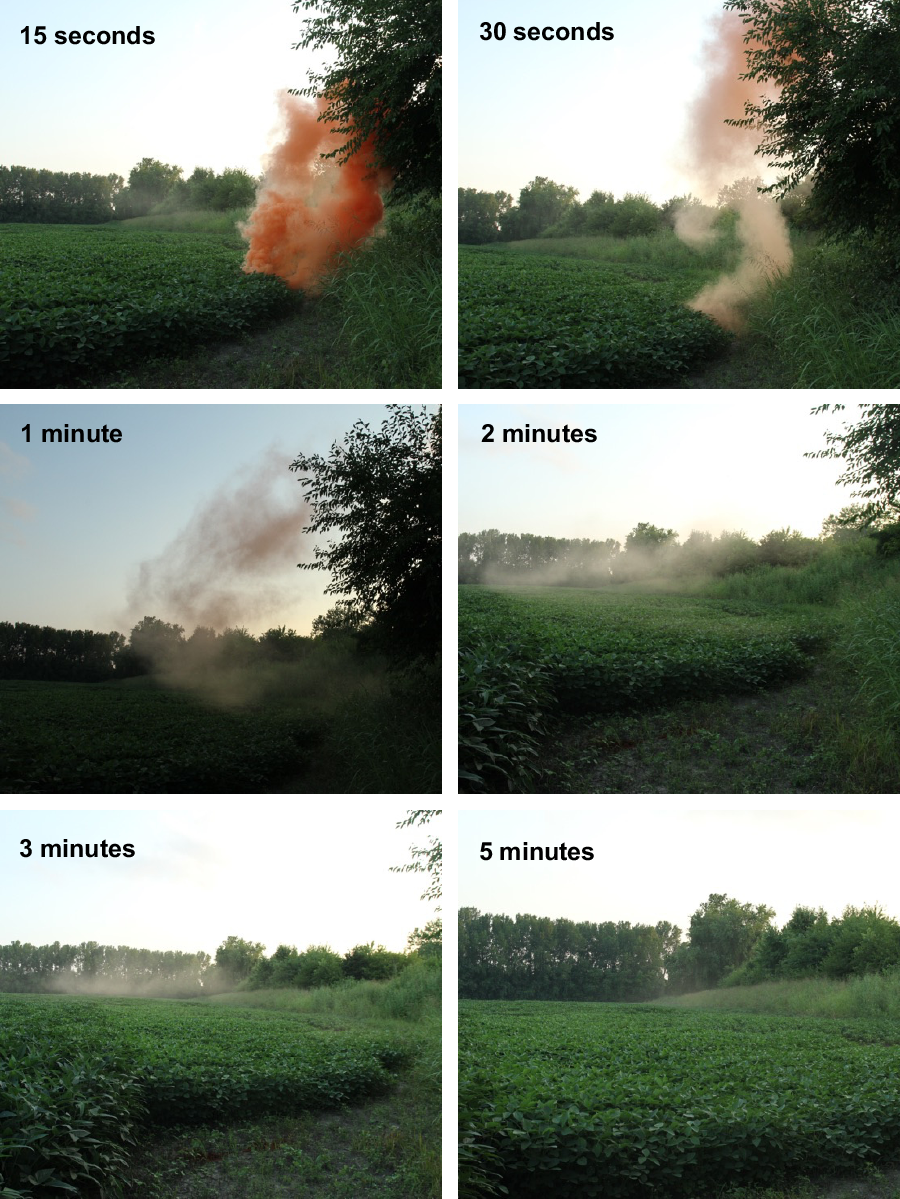
Figure 3. A time-lapse series following the release of a smoke bomb at a soybean field adjacent to a pipe river. The river is on the other side of the distal tree line. The visible plume first moved vertically. As the plume reached the height of the tree line, between 30 s and 1 min, it began sinking, which is likely the result of being incorporated into a cooler air stream. The particulate did not disperse but moved as a dust cloud to the low point in the field, where it remained visible for 3 min. (These particular smoke bombs, Enola Gaye smoke grenades, are designed to emit an observable plume for 90 s.)
Removal of Pesticides from the Atmosphere
Pesticides suspended in the atmosphere are removed via five mechanisms: degradation of a stable air mass or drainage system, dry deposition, wet deposition, chemical degradation, and photochemical degradation (Glotfelty and Caro Reference Glotfelty and Caro1975). Virtually all airborne particles undergo one or a combination of these factors for their removal from the atmosphere.
In the same field where a smoke bomb was released to illustrate cool air drainage, and a few meters into the nearest tree line, sporadic damage that resembled dicamba and glyphosate injury (Figure 4) was observable at heights similar to those reached by the smoke plume in Figure 3. One possible explanation for the observed injury is that the pesticides moved into the air following application and in a similar fashion to the initial vertical rising of the smoke bomb. Another possibility is that the pesticides may have volatilized into the air. Regardless of how the pesticide moved into the air, horizontal winds likely moved the chemicals into the tree line where the leaf surfaces could have served as an obstruction to the horizontal air movement, allowing dry deposition of the chemical.

Figure 4. A few meters into the nearest tree line from where the smoke bomb was released (Figure 3), sporadic damage that resembled dicamba and glyphosate injury was observable in the trees. Red arrows point toward dicamba and glyphosate symptoms. (B) Enlarged image of injury resembling leaf cupping or leaf rolling, typical of dicamba. (C) Enlarged photograph of the generalized chlorosis and necrosis of the younger leaves associated with glyphosate injury.
Dry deposition is the settling of pesticides that have sorbed onto suspended particulate matter in the atmosphere (Majewski and Capel 1996). Wet deposition occurs when particles are scavenged by raindrops and redistributed to the earth’s surface. This is a rapid and predominant pathway for removal of pesticides from the atmosphere (Glotfelty and Caro Reference Glotfelty and Caro1975; Majewski and Capel 1996). Bulk deposition samplers are a common method of collecting wet and dry deposition samples for downstream analysis (Messing et al. Reference Messing, Farenhorst, Waite and Sproull2014; Waite et al. Reference Waite, Sommerstad, Grover, Kerr, Westcott and Irvine1995, Reference Waite, Cessna, Gurprasad and Banner1999). Studies using either wet deposition or bulk deposition have been used to identify potential relationships between concentrations of pesticides removed from the atmosphere and usage of those pesticides within that region (Farenhorst et al. Reference Farenhorst, Andronak and McQueen2015; Goolsby et al. Reference Goolsby, Thurman, Pomes, Meyer and Battaglin1997; Thurman and Cromwell Reference Thurman and Cromwell2000; Waite et al. Reference Waite, Cessna, Grover, Kerr and Snihura2002, Reference Waite, Cessna, Grover, Kerr and Snihura2004). In a study of rainfall samples collected from 81 sites in the Midwest and Northeast United States in 1990 and 1991, Goolsby et al. (Reference Goolsby, Thurman, Pomes, Meyer and Battaglin1997) found that peak concentrations of atrazine and alachlor were detected in May through July and deposition was highest in the corn belt and decreased with distance removed from the corn belt. Waite et al. (Reference Waite, Cessna, Grover, Kerr and Snihura2004) found a similar relationship between dicamba and bulk deposition in Canadian prairies, in which dicamba concentrations peaked in June at ranges from 0.5 ng m−2 d−1 to approximately 1.7 ng m−2 d−1 depending on location and year. However, research is still needed to determine what concentration of dicamba (or any pesticide of interest) must be deposited from the atmosphere to result in injury of sensitive species.
Pesticide degradation is another mechanism that can act to remove chemicals from the atmosphere. Glotfley (Reference Glotfelty1978) concluded that compounds able to strongly absorb solar wavelengths may be more likely to rapidly decompose. Factors that control the atmospheric half-life of a pesticide are difficult to study but likely important in understanding why some pesticides are more persistent in the atmosphere while others are not.
Practical Applications
Elaborate and extensive studies have been and continue being conducted on physical drift of pesticides (Alves Reference Alves, Kruger, Paulo, da Cunha, Vieira, Henry, Obradovic and Grujic2017; Carlson et al. Reference Carlsen, Spliid and Svensmark2006; Johnson et al. Reference Johnson, Roeth, Martin and Klein2006; Vangessel Reference Vangessel and Johnson2005; Vieira et al. Reference Vierra, Butts, Rodrigues, Schleier, Fritz and Kruger2020). Producers and agricultural professionals have readily adopted the outcome(s) from many of those findings whether it be nozzle size, drift reduction agents, and so on (Bish and Bradley Reference Bish and Bradley2017). To achieve similar results with regards to secondary movement of pesticides, producers and agricultural professionals will need more education on secondary pesticide movement and new best management practices and tools to adopt. The concepts of cool air drainage and inversion can easily be demonstrated with smoke bombs (Figures 3 and 5) and/or liquid nitrogen, which can provide a good example of cool air sinking and moving. Applicators need to understand that topography and obstructions in fields will influence formation of stable air masses. An inversion may be occurring in one field and not yet formed in a nearby field (Bish and Bradley Reference Bish, Guinan and Bradley2019b). Inversion forecasting tools continue to be developed. However, developing accurate tools that predict inversions near the ground, reliably and across multiple topographies is a difficult task (Bish et al. Reference Bish, Guinan and Bradley2019b).
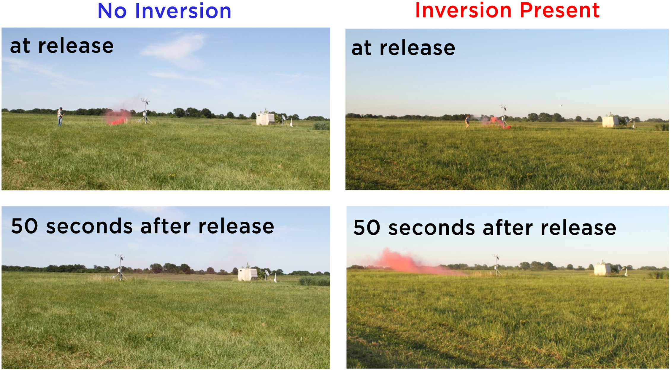
Figure 5. Smoke bombs released at the same site in Columbia, Missouri (2017), during unstable, noninversion conditions (approximately 4:00 P.M.) and inversion conditions (approximately 7:30 P.M.). The smoke plume has dissipated by 50 s following release during noninversion conditions while the plume remained intact during stable conditions.
From a research perspective, more consideration needs to be given to all of the potential effects of wind. Measuring wind speed at boom height at the time of application seems acceptable for concerns about physical drift. However, with regard to secondary transport of pesticides, is there a height about ground level for which wind speeds can be measured and used to predict the likelihood of an application remaining on target?
The U.S. Environmental Protection Agency published a study in 2006 showing that some agricultural areas pose higher risks for off-target pesticide movement (Pfleeger Reference Pfleeger, Olszyk, Burdick, King, Kern and Fletcher2006). The percent of land in agriculture, diversity of crops, rates of herbicide use in a given area, and frequency of high winds were all factors that affected the risks of physical drift to nearby sensitive species (Pfleeger Reference Pfleeger, Olszyk, Burdick, King, Kern and Fletcher2006). Perhaps a similar study is warranted that considers the effects of a lack of wind on secondary pesticide movement.
With increased public awareness of pesticides, the release of multiple herbicide-resistant traits, and concerns over environmental fate, it is essential we not become complacent in our assumptions about secondary movement but advance our understanding above what is currently known.


 Open access