2.1. Problem formulation

We formulate our flow configuration in the same framework as Williamson et al. (Reference Williamson, Armfield, Kirkpatrick and Norris2015) and their simulations of stationary radiatively heated open channel flow. A similar framework has been used for the destratifying open channel simulations of Kirkpatrick et al. (Reference Kirkpatrick, Williamson, Armfield and Zecevic2019) and Kirkpatrick et al. (Reference Kirkpatrick, Williamson, Armfield and Zecevic2020). A schematic of the flow is presented in figure 1. The flow is periodic in the streamwise ($x$) and spanwise ($y$) directions with no-slip and free-slip adiabatic bottom and top boundaries, respectively, and driven by a constant pressure gradient in $x$. The flow is heated through a depth varying volumetric heat source $q_I(z)$ on the principle of Beer–Lambert's law, defined as

(2.1)\begin{equation} q_I(z) = I_s\alpha {\rm e}^{(z-\delta)\alpha}, \end{equation}

where $I_s$ is the radiant surface heat flux, $\alpha$ is the absorption coefficient and $\delta$ is the channel height. Hence we can define domain-averaged mean heat source and normalized heat flux terms

(2.2a,b)\begin{equation} \langle q \rangle = \frac{1}{\delta}\int_0^{\delta}q_I(z)\,{\rm d}z, \quad q_N = \frac{1}{\delta^{2}}\int_0^{\delta}(\langle q \rangle-q_I(z))(z-\delta)\,{\rm d}z. \end{equation}

The dimensional temperature $\varTheta$ at time $t$ is decomposed into the statistically steady temperature fluctuation deviating from a domain-averaged mean, defined as

(2.3)\begin{equation} \varTheta(\boldsymbol{x},t) = \varTheta(\boldsymbol{x},t)' + \langle \varTheta(t) \rangle \end{equation}

and, under the assumption that no heat is lost through the boundaries, it follows that

(2.4)\begin{equation} \frac{\partial \langle \varTheta(t) \rangle}{\partial t} = \frac{\langle q \rangle}{\rho_0 C_p}, \end{equation}

where $\rho _0$ is the reference fluid density and $c_p$ is the specific heat. By defining the initial equilibrium friction velocity $u_{\tau,0}$ and channel depth $\delta$ as the characteristic velocity and length scales, respectively, we can then define a characteristic temperature scale

(2.5)\begin{equation} \varTheta_N = \frac{q_N\delta}{\rho_0 c_p u_{\tau,0}}. \end{equation}

Hence we can define a non-dimensional temperature and heat source

(2.6a,b)\begin{equation} \theta(\boldsymbol{x},t) = \frac{\varTheta(\boldsymbol{x},t) - \langle \varTheta(t) \rangle}{\varTheta_N}, \quad q(z) = \frac{q_I(z) - \langle q \rangle}{q_N}. \end{equation}

Our flow is then fully defined by four non-dimensional parameters: the initial friction Reynolds number $Re_{\tau,0}$; the Prandtl number $Pr$; the turbidity profile $\alpha \delta$; and an initial bulk stability parameter $\lambda _0$, defined as

(2.7a–d)\begin{equation} Re_{\tau,0} = \frac{u_{\tau,0}\delta}{\nu}, \quad Pr = \frac{\nu}{\kappa}, \quad \alpha \delta, \quad \lambda_0 = \frac{\delta}{\mathcal{L}}, \end{equation}

where $\nu$ and $\kappa$ are the kinematic viscosity and thermal diffusivity, respectively. Also note that in our framework, $\alpha \delta \Rightarrow \infty$ is analogous to a heat flux at the top surface similar to the simulations of Taylor et al. (Reference Taylor, Sarkar and Armenio2005). The stability of our flow is defined in the Monin–Obhukov framework as the ratio of the domain confinement scale $\delta$ to bulk Obhukov length $\mathcal {L}$ defined as

(2.8)\begin{equation} \mathcal{L} = \frac{u_{\tau,0}^{3}}{g\beta I_s/\rho_0 C_p} \left( \frac{1}{2} - \frac{1}{\alpha\delta}\right)^{{-}1}, \end{equation}

where $g$ is the gravitational acceleration and $\beta$ is the coefficient of thermal expansion. Note that $\mathcal {L}$ is analogous to the standard definition of the Obhukov length $L = u_{\tau }^{3}/\kappa b_*$ where $b_*$ is the surface buoyancy flux (Flores & Riley Reference Flores and Riley2011). Thus we define our non-dimensional buoyancy scale as

(2.9)\begin{equation} b = \lambda_0 \theta. \end{equation}

We non-dimensionalize time around the initial advection time scale $T_{\tau,0} = \delta / u_{\tau,0}$ such that

(2.10)\begin{equation} t = T/T_{\tau,0}, \end{equation}

where $T$ is the dimensional time. Thus, under the Oberbeck–Boussinesq assumption, the non-dimensional governing equations for our flow are

(2.11)\begin{gather} \boldsymbol{\nabla}\boldsymbol{\cdot}\boldsymbol{u} = 0, \end{gather}

(2.12)\begin{gather}\frac{\partial \boldsymbol{u}}{\partial t} + \boldsymbol{u}\boldsymbol{\cdot}\boldsymbol{\nabla}\boldsymbol{u} ={-} \boldsymbol{\nabla} p + \frac{1}{Re_{\tau,0}}\nabla^{2}\boldsymbol{u} + b\boldsymbol{e}_z +\boldsymbol{e}_x, \end{gather}

(2.13)\begin{gather}\frac{\partial b}{\partial t} + \boldsymbol{u} \boldsymbol{\cdot} \boldsymbol{\nabla} b = \frac{1}{Pr Re_{\tau,0}}\nabla^{2}b + \lambda_0 q, \end{gather}

with our boundary and initial conditions explicitly defined as

(2.14)\begin{gather} z = 0; \quad u=v=w=0, \quad \frac{\partial b}{\partial z} = 0, \end{gather}

(2.15)\begin{gather}z = \delta; \quad \frac{\partial u}{\partial z}=\frac{\partial v}{\partial z}=w=0, \quad \frac{\partial b}{\partial z} = 0, \end{gather}

(2.16)\begin{gather}t = 0; \quad b = 0. \end{gather}

We have selected this open channel flow configuration for three reasons. Firstly, the use of an adiabatic bottom boundary has been shown to ensure that while the bulk flow becomes stratified, the near-wall turbulence structure remains relatively unchanged by the effects of buoyancy (Taylor et al. Reference Taylor, Sarkar and Armenio2005; Williamson et al. Reference Williamson, Armfield, Kirkpatrick and Norris2015), allowing for simulations to be run at significantly higher levels of buoyancy strength than isoflux or fixed buoyancy boundary conditions where the relaminarization and collapse of turbulence inherently occurs at the wall (Flores & Riley Reference Flores and Riley2011; García-Villalba & del Álamo Reference García-Villalba and del Álamo2011; Deusebio et al. Reference Deusebio, Caulfield and Taylor2015; Zhou et al. Reference Zhou, Taylor and Caulfield2017a). Secondly, relative to a surface flux boundary condition, use of the volumetric heat source shifts the pycnolcine deeper into the channel away from the upper boundary, creating an appreciable region in the central bulk flow of significantly stronger stratification (Williamson et al. Reference Williamson, Armfield, Kirkpatrick and Norris2015). This subsequently allows us to access regimes of lower $Fr$ farther away from the top boundary, where confinement effects may influence mixing dynamics (Flores, Riley & Horner-Devine Reference Flores, Riley and Horner-Devine2017). Thirdly, our direct numerical simulation (DNS) configuration of a stratified open channel flow heated through radiative surface heating is a canonical representation of stratified river flow and in particular the regulated river flows in inland Australia, where the accurate estimation and prediction of diapycnal mixing remains an important task (Williamson et al. Reference Williamson, Armfield, Kirkpatrick and Norris2015; Kirkpatrick et al. Reference Kirkpatrick, Williamson, Armfield and Zecevic2019).

Figure 1.

Schematic diagram of the flow configuration; the domain is periodic in $x$ and $y$.

2.2. Notation and presentation of statistics

Within our temporally varying and vertically inhomogeneous flow, we define that any flow variable at a spatial location $\boldsymbol {x}$ and time $t$ can be decomposed into a horizontally averaged mean and fluctuating components denoted with an overbar and prime, respectively, such that

(2.17)\begin{equation} f(\boldsymbol{x},t) = \bar{f}(z,t) + f'(\boldsymbol{x},t) \end{equation}

and where the mean at a vertical location of $z$ is calculated through a volumetric integral across the horizontal plane at time $t$, as follows:

(2.18)\begin{equation} \bar{f}(z,t) = \frac{1}{L_x L_y} \int_0^{L_x} \int_0^{L_y} f(\boldsymbol{x},t) \,{\rm d}\kern0.7pt x\,{\rm d}y. \end{equation}

Similarly, we define that unless otherwise explicitly stated, it is implicit that flow statistics composed out of the velocity and buoyancy fields (e.g. $\epsilon _K,E_K,S,N$ etc) are presented as horizontal averages of that quantity at location $z$ and time $t$ as defined in (2.18).

2.3. DNS

Equations (2.11), (2.12), (2.13) were solved using a fractional-step finite-volume solver as outlined in Armfield et al. (Reference Armfield, Morgan, Norris and Street2003) and Williamson et al. (Reference Williamson, Armfield, Kirkpatrick and Norris2015). The advective spatial derivatives are discretized using fourth-order central differencing, whilst other spatial derivatives are calculated using second-order central differencing. Cell-face velocities are calculated using Rhie–Chow momentum interpolation and the time advancement is performed using a second-order Adams–Bashforth scheme.

We present our simulation parameters in table 1. Our simulations cover two friction Reynolds numbers, $Re_{\tau,0}=400,900$. As we are primarily interested in the low $Fr$ (high $Ri_g)$ regimes, our simulations cover a range of stability parameters, from moderately to extremely stable $(\lambda _0 = 0.5 - 5)$. We limit all simulations to $Pr = 1$ for numerical efficiency and set $\alpha \delta = 8$ for all simulations with a single control case of $\alpha \delta = 16$.

Table 1.

List of DNS performed, and relevant parameters.

Following past studies of stratified wall-bounded turbulence (García-Villalba & del Álamo Reference García-Villalba and del Álamo2011; Deusebio et al. Reference Deusebio, Caulfield and Taylor2015; Williamson et al. Reference Williamson, Armfield, Kirkpatrick and Norris2015), we discretize our domain as follows. For all simulations the streamwise and spanwise grid size in initial viscous wall units is kept constant at $\Delta x_0^{+} = 5$ and $\Delta y_0^{+} = 2.5$. The vertical grid size for the $Re_{\tau,0}=400$ simulations is logarithmically stretched from $\Delta z_0^{+} = 0.4$ at the wall to $\Delta z_0^{+} = 4$ at $z = 0.25$ where it stays constant to the half-channel height $z = 0.5$. The vertical grid spacing in the top half of the channel is then set as symmetrical about the midpoint axis to ensure accurate resolution of viscous near-surface mechanics (Calmet & Magnaudet Reference Calmet and Magnaudet2003). A similar procedure for the vertical grid size of the $Re_{\tau,0}=900$ simulations was employed with a further refinement of $\Delta z_0^{+} = 2.5$ in the bulk of the flow. To maintain accurate resolution of the viscosity affected near-wall and near-surface regions, we ensure that we have more than 10 grid points within a $\Delta z_0^{+} = 10$ distance from either boundary.

We keep the domain size constant at $L_x \times L_y \times L_z = 2 {\rm \pi}\delta \times {\rm \pi}\delta \times \delta$ across all simulations. We acknowledge that the size of the domain may affect the intermittent regime where laminar and turbulent patches coexist, as it has been shown that a smaller domain often leads to earlier laminarization for the same set of bulk parameters and can exhibit strong temporal intermittency (Flores & Riley Reference Flores and Riley2011; García-Villalba & del Álamo Reference García-Villalba and del Álamo2011; Brethouwer, Duguet & Schlatter Reference Brethouwer, Duguet and Schlatter2012; Deusebio et al. Reference Deusebio, Caulfield and Taylor2015). In this study, however, we are primarily interested in instantaneously correlating local turbulent mixing properties to appropriate local non-dimensional parameters within fully turbulent regions of the flow. Furthermore, our adiabatic bottom boundary condition ensures that the near-wall region remains fully turbulent, hence we do not expect the domain size to significantly influence the results presented in this study.

The initial simulation field is of fully developed statistically stationary neutral open channel flow at a given $Re_{\tau,0}$. For all simulations we then initialize the isothermal buoyancy field $b = 0$ at $t = 0$ and simultaneously switch on the volumetric heat source and the effects of buoyancy. All simulations have been run for $t_{{final}} = 10$ time units. For all simulations, transient data has been recorded at intervals of $\Delta t = 0.02$ time units to ensure accurate representation of temporal effects within the flow.

3.1. Qualitative description and local parameter range

A defining feature of our DNS configuration is that as the channel transitions from a neutral to stratified state, the local flow at any given vertical location $z$ evolves through a broad range of non-dimensional parameters such that, at any point in time, the flow contains regions of both high and low $Fr$ simultaneously. This creates a data set that traverses a variety of energetic regimes within a single simulation and where the flow, both mean and fluctuating, evolves in a relatively natural way without external imposition. We briefly present the local parameter range available within our data set through figure 2 showing the temporal evolution of $Fr$ and $Re_B$ as a function of $z$ for case R900L2 which shows behaviour typical of our flow, where we redefine

(3.1a,b)\begin{equation} Fr = \frac{\epsilon_K}{N E_K}, \quad Re_B = \frac{\epsilon_K}{N^{2} \nu}, \end{equation}

where $\epsilon _K = \nu (\partial u_i'/\partial x_j)^{2}$, $E_K = 1/2(\overline {u_i'u_i'})$ and $N = (\partial \bar {b}(z)/\partial z)^{1/2}$. From figure 2(a) we observe that the flow obtains an $Fr$ range that encapsulates all three energetic mixing regimes proposed by GV19. Of particular interest is that within the central portion of the channel, $Fr$ stabilizes within approximately one eddy turnover unit ($t \approx 1$) and obtains an appreciable depth range for the so-called ‘moderately stratified regime’ where $Fr = O(1)$ in an energetically ‘quasi-stationary’ state such that turbulent properties adapt rapidly to the evolving buoyancy gradient $N$ in order to obtain energetic equilibrium. As outlined in § 1, in previous numerical studies this regime is only often temporarily traversed as a transient state and subsequently there is a lack of data points in the available literature within this regime. As such our flow and extensive data set of $Fr = O(1)$ allows us to examine the mixing properties and scaling relationships within this regime in much greater detail than has been previously reported.

Figure 2.

Evolution in time of key local parameters as a function of $z$ for case R900L2. (a) Turbulent Froude number $Fr$, vertical dotted lines left to right represent $Fr = 0.02$ (as the upper limit for the strongly stratified regime outlined in Lindborg Reference Lindborg2006) and $Fr = 1$; (b) buoyancy Reynolds number $Re_B$, vertical dotted line represents $Re_B = 1$.

Although the flow achieves $Fr<0.02$ close to the free surface, our simulations are not able to access the ‘strongly stratified regime’ in the same sense as outlined in Billant & Chomaz (Reference Billant and Chomaz2001) or Brethouwer et al. (Reference Brethouwer, Billant, Lindborg and Chomaz2007). This is made evident in figure 2(b), which demonstrates that for our flow configuration as we approach the free surface, the stratification grows stronger and a reduction in $Fr$ inevitably leads to a reduction in $Re_B$, leading to the relaminarization of the flow. Subsequently at our parameter range, regions within our flow of very low $Fr$ are more indicative of a diffusive regime as described by Brethouwer et al. (Reference Brethouwer, Billant, Lindborg and Chomaz2007), where $Re_B <1$ and the flow is dominated by viscous effects and strong vertical shearing at large scales.

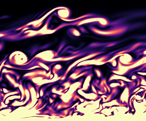
This is made clear if we consider the instantaneous visualizations of the buoyancy $b$ and enstrophy $|\boldsymbol {\omega }^{2}|$ fields in the vertical ($x,z$) plane at $t = 5$ in figure 3 for case R900L2. We can clearly observe that the flow is separated into three distinct regimes relative to the vertical coordinate $z$: a lower near-wall regime, where due to the adiabatic boundary condition the boundary layer turbulence structure remains relatively unchanged by the effects of stratification; a central region within which turbulent structures exhibit the characteristic ‘lean’ of sheared stratified turbulence and where we observe the formation of distinctly classic Kelvin–Helmholtz instability (KHI) overturning structures within the shear layer, causing highly vigorous and energetic mixing; an upper quasi-laminar or diffusive regime where turbulence is essentially suppressed by the effects of buoyancy and separated by a sharp buoyancy interface that experiences sporadic overturning by turbulent structures. Thus, the turbulence structure visually observed in figure 3 corresponds closely to the three regimes defined by $Fr$ and $Re_B$ in figure 2.

Figure 3.

Instantaneous flow visualizations in the vertical ($x,z$) plane at $t = 5$ for case R900L2 of (a) the buoyancy field $b$ and (b) enstrophy field $|\boldsymbol {\omega }^{2}|$. Flow is moving left to right.

3.2. A note on the mixing efficiency

Throughout this study we defer to a definition of the instantaneous mixing efficiency through $R_f$ and $\varGamma$ as defined in Ivey & Imberger (Reference Ivey and Imberger1991),

(3.2a,b)\begin{equation} R_f = \frac{B}{B+\epsilon_K}, \quad \varGamma = \frac{R_f}{1-R_f} = \frac{B}{\epsilon_K}, \end{equation}

where $B = \overline {-b'w'}$ is the buoyancy flux. The vertical buoyancy flux, however, not only incorporates the small-scale irreversible mixing rate (the quantity of interest) but also large-scale reversible stirring processes (Caulfield & Peltier Reference Caulfield and Peltier2000; Peltier & Caulfield Reference Peltier and Caulfield2003). As such, for linearly stratified flows a more robust definition of the irreversible mixing rate is usually defined through the destruction rate of buoyancy variance $\chi$ (Maffioli et al. Reference Maffioli, Brethouwer and Lindborg2016; Venayagamoorthy & Koseff Reference Venayagamoorthy and Koseff2016; de Bruyn Kops & Riley Reference de Bruyn Kops and Riley2019; Howland, Taylor & Caulfield Reference Howland, Taylor and Caulfield2020), where

(3.3)\begin{equation} \chi = \frac{\kappa}{N^{2}}\left(\overline{\frac{\partial b'}{\partial x_j}}\right)^{2}. \end{equation}

For $\chi$ to accurately represent the irreversible conversion of kinetic to available potential energy, a fundamental condition is that the local buoyancy period $N(z)$ must be invariant in both space and time (Caulfield Reference Caulfield2020), a condition that is inherently unsatisfied within our temporally evolving inhomogeneous channel flow.

An alternative framework is through the adiabatic resorting of the buoyancy in the $z_*$ coordinate space of Winters et al. (Reference Winters, Lombard, Riley and D'Asaro1995) to obtain an irreversible mixing rate $\mathcal {M}$ and subsequently an irreversible mixing efficiency $\eta = \mathcal {M}/(\mathcal {M}+\epsilon _K)$ (Caulfield & Peltier Reference Caulfield and Peltier2000). In past studies, Zhou et al. (Reference Zhou, Taylor, Caulfield and Linden2017b) and Smith, Caulfield & Taylor (Reference Smith, Caulfield and Taylor2021) have shown that the framework may be also applied to inhomogeneous shear flows to evaluate irreversible mixing across a midplane shear interface through appropriate spatial and temporal integration over the shear layer. However, in stratified open-channel flow where we are interested in investigating the correlation between mixing efficiency and local flow parameters across a broad range of vertical locations, rather than a single central shear layer, the $z_*$ framework presents obvious limitations. We note, the aim of this study is not to quantify an exact measure of the irreversible mixing efficiency, but rather to investigate its behavioural trends across different mixing regimes and the subsequent implications on the relationships between varying non-dimensional parameters at a given vertical location. Furthermore, as shown in Venayagamoorthy & Koseff (Reference Venayagamoorthy and Koseff2016), we expect that in the weakly and moderately stratified regimes the differences in the definitions of mixing efficiency to be relatively small and the qualitative behaviour to remain similar. As such, our definition of mixing efficiency through (3.3) still accurately captures the dynamics of interest in our study.

5.1. $Fr - \varGamma$ framework and moderately stratified regime scaling

To begin we first explicitly test the novel $\varGamma - Fr^{-1}$ scaling relationship derived in GV19 for the $Fr = O(1)$ regime. The authors argue that the pertinent time scales for $B$ and $\epsilon _K$ are the buoyancy and inertial time scales $T_N = 1/N$ and $T_L = E_K/ \epsilon _K$, respectively. Under the assumption of a stationary linearly stratified flow they obtain

(5.1a,b)\begin{equation} B \sim \chi \sim \frac{w'^{2}}{T_N}, \quad \epsilon_K \sim \frac{w'^{2}}{T_L}. \end{equation}

Thus they obtain the new scaling for the irreversible mixing coefficient $\varGamma = B/\epsilon _K \sim \chi /\epsilon _K \sim T_L/T_N = Fr^{-1}$. For the purpose of generality we make one further assumption, that at $Fr = O(1)$ the separation of vertical and horizontal velocity scales is still relatively small and hence we can approximate $w'^{2} \sim E_K$. We can thus rewrite (5.1) in the classic form of velocity and length scales $\epsilon \sim u^{3}/l$ as

(5.2a,b)\begin{equation} B \sim \chi \sim \frac{E_K}{T_N} \sim \frac{E_K^{3/2}}{L_{N}}, \quad \epsilon_K \sim \frac{E_K}{T_L} \sim \frac{E_K^{3/2}}{L_{I}}, \end{equation}

where

(5.3a,b)\begin{equation} L_{N} = \frac{E_K^{1/2}}{N}, \quad L_{I} = \frac{E_K^{3/2}}{\epsilon_K}. \end{equation}

Here $L_{N}$ is an energetic buoyancy length scale constructed as a result of dimensional analysis and can be taken to represent the conceptual size of large energy-containing eddies when the effects of buoyancy are significant. Now $L_N$ has also been shown to be an accurate indicator of the size of overturns when $Fr < 1$ (Mater et al. Reference Mater, Schaad and Venayagamoorthy2013). Here $L_{I}$ is the well known inertial energy-containing turbulent length scale (Pope Reference Pope2000). Such that for the moderately stratified regime we obtain $\varGamma = B/\epsilon _K \sim \chi /\epsilon _K \sim L_{I}/L_{N} = Fr^{-1}$, the same scaling as GV19. If considered in the context of the strongly stratified turbulence theory of Billant & Chomaz (Reference Billant and Chomaz2001) and Lindborg (Reference Lindborg2006) it can be readily seen that $L_{N}$ and $L_{I}$ have physical analogues in the vertical and horizontal integral scales $l_v \sim u_h/N$ and $l_h \sim u_h^{3}/\epsilon _K$, respectively, where $u_h$ is the horizontal velocity scale.

As discussed in § 3, the definition of $\chi$ as an irreversible mixing rate in the derivation above is not equivalent to that of an instantaneous local $\chi (z)$ as measured within our flow, hence, and without loss of generality, we explore these scaling proposals through the buoyancy flux $B$ instead. Figure 5(a) shows $B$ normalized by $E_K^{3/2} /L_{N}$ as function of time at a vertical location of $z = 0.5$, corresponding to a location in the flow where $Fr = O(1)$ and $Re_B \gg O(1)$ for all simulations. For the proposed scaling to hold, we expect the former ratio to approach a constant value of $O(1)$. We further note that it is sufficient to show the $B$ scaling alone to validate the $\varGamma \sim Fr^{-1}$ assumption; as it can readily be shown that $\epsilon _K / (E_K^{3/2}/L_{I}) = (\epsilon _K /E_K^{3/2}) /(\epsilon _K /E_K^{3/2}) = 1$.

Figure 5.

Buoyancy flux $B$ normalized by $E_K^{3/2} /L_{N}$, (a) as a function of time $t$ for all simulations at a vertical location of $z = 0.5$, (b) as a function of the turbulent Froude number $Fr$ presented as a two-dimensional probability density function (p.d.f.) for $t>1$ and $0.2 \leqslant z \leqslant 0.8$. Vertical dashed lines indicate $Fr = 0.3$ and $Fr = 1$. Dashed horizontal line in both figures indicates an empirical constant of 0.08.

In agreement with our analysis in § 4 we observe that the scaling does not hold for $t < 1$ during the transient adjustment period, past which the results clearly show an agreement with the scaling in (5.2) such that $B / (E_K^{3/2} /L_{N})$ approaches a constant value of approximately $0.08$ across all simulations and appears invariant in time. When considered in the context of our temporally inhomogeneous flow where not only the turbulent properties but also the background stratification $N^{2}$ is evolving in time, the result implies that the above scaling for $B$ in (5.2) is both valid and relatively robust. This is further made evident in figure 5(b) which shows the two-dimensional p.d.f. of $Fr$ and the ratio $B / (E_K^{3/2} /L_{N})$ for all simulations. Due to the initial time dependence observed in § 4 we exclude the data for $t<1$ in the construction of the p.d.f. Furthermore, as the confinement effects of the top and bottom boundaries are outside the scope of this study we also exclude the data for $z<0.2$ and $z>0.8$. The vertical limits of $z=0.2$ and $z=0.8$ have been chosen as the approximate values within which fully developed open channel flow has been shown to obtain local energetic equilibrium (Williamson et al. Reference Williamson, Armfield, Kirkpatrick and Norris2015; Kirkpatrick et al. Reference Kirkpatrick, Williamson, Armfield and Zecevic2019). It is indeed clear from the results that $B / (E_K^{3/2} /L_{N}) \approx 0.08$ and remains constant only for a regime within the bounds of $0.3 \lesssim Fr \lesssim 1$, presenting further strong evidence for the argument of GV19 for the existence of a separate intermediate energetic regime that exists in a quasi-stationary state and not as a transient transition between the weakly and strongly stratified regimes. We note that the value of $Fr = 0.3$ is in direct agreement with the transitional value observed in MBL16 towards the asymptotic $\varGamma$ regime within their study, suggesting some level of universality to this transitional value.

We now turn our attention to the $Fr$-based parameterization of the mixing efficiency. Figure 6(a) shows the two-dimensional p.d.f. of $Fr$ and $\varGamma$ for all simulations constructed out of the data within the range of $t>1$ and $0.2 \leqslant z \leqslant 0.8$.

Figure 6.

(a) Two-dimensional p.d.f. of the turbulent Froude number $Fr$ and the mixing coefficient $\varGamma$ constructed out of the instantaneous data of all simulations within the range of $t>1$ and $0.2 \leqslant z \leqslant 0.8$. The axes on the insert within the figure are presented on a linear scale. (b) The $Fr$ bin-averaged mixing coefficient $\langle \varGamma \rangle$ plotted against bins of corresponding turbulent Froude number $\langle Fr \rangle$ for all data points within $t>1$ and $z>0.2$. Solid lines indicate the proposed scaling of MBL16 and GV19 as well as empirically observed $\varGamma = 0.3$. Vertical dashed lines indicate $Fr = 0.3$ and $Fr = 1$.

From the results we observe that $\varGamma$ collapses well across all three energetic regimes and respective scaling relationships proposed by MBL16 and GV19. Although we only access a very small section of the weakly stratified regime, we observe a distinct $Fr^{-2}$ slope developing in the high $Fr$ range similar to that observed in the Couette flow studies of Zhou et al. (Reference Zhou, Taylor and Caulfield2017a,Reference Zhou, Taylor, Caulfield and Lindenb). Crucially, in agreement with our analysis above, we observe that within a range of $0.3 \lesssim Fr \lesssim 1$ where the majority of our data is concentrated, $\varGamma$ collapses across all simulations and depths with a distinct $Fr^{-1}$ scaling, providing further strong evidence for the existence of a distinctly separate intermediate regime as proposed by GV19. Unlike MBL16, however, who find that $Fr = 0.3$ corresponds to a peak in mixing efficiency, we observe no non-monotonic behaviour in $\varGamma$, rather the transition at $Fr = 0.3$ corresponds to a saturation of the mixing efficiency, with $\varGamma$ displaying independence of $Fr$ and trending towards an empirically observed asymptotic value of $\varGamma \approx 0.3$. The asymptotic value being significantly higher than the upper limit of $0.2$ proposed by Osborn (Reference Osborn1980), is more reminiscent of the higher values of cumulative mixing efficiency seen in studies of KHI-induced mixing (Salehipour & Peltier Reference Salehipour and Peltier2015; Mashayek, Caulfield & Peltier Reference Mashayek, Caulfield and Peltier2017; Salehipour et al. Reference Salehipour, Peltier and Caulfield2018), seemingly in agreement with our visual observations of highly energetic KHI-driven mixing events within our flow.

With further decreasing $Fr$ we observe a significant amount of scatter in the data. This can be explained as the flow transitions towards the diffusive regime and both $B$ and $\epsilon _K$ grow very small and a minor change in either of the two quantities causes large variation in $\varGamma$. Additionally, as has been reported in the study García-Villalba & del Álamo (Reference García-Villalba and del Álamo2011), channel flow within this regime becomes increasingly affected by the propagation of internal gravity waves as well as counter-gradient fluxes resulting from convective instabilities in the flow (Taylor et al. Reference Taylor, Sarkar and Armenio2005). This results in instantaneous measurements of $B$ becoming strongly susceptible to contamination from these reversible processes, subsequently causing our measurements of $\varGamma$ within this regime to show significant scatter about its asymptotic mean value. Furthermore, as discussed in Venayagamoorthy & Koseff (Reference Venayagamoorthy and Koseff2016) the presence of the counter-gradient fluxes may cause the observed saturated mean value of $\varGamma = 0.3$ to underestimate the true irreversible mixing efficiency. However, as can be observed from the insert in figure 6(a) which presents the same data on a linear–linear axes, the observed frequency of counter-gradient fluxes is relatively negligible in comparison with the full data set. As such the significant takeaway from the results presented within this regime is not the precise value for the saturated mixing efficiency but rather the observation that $\varGamma$ appears to grow independent of $Fr$ within this regime.

To investigate this further we sort and average our instantaneous measurements of horizontal plane measurements of $\varGamma (z,t)$ across bins of constant $Fr$ to obtain the binned data set of $\langle \varGamma \rangle$. Avoiding near-wall mechanics we consider all data for $z>0.2$ and $t>1$. We note that for this case we include the data near the free-surface boundary to highlight the departure point from the saturated regime towards the diffusive regime. Figure 6(b) shows $\langle \varGamma \rangle$ plotted against bins of corresponding $\langle Fr \rangle$ for all simulations under the conditions described above. A colour bar depicting $\langle Re_B \rangle$ is also shown for reference. When presented in this manner, it becomes clear that for $Fr \lesssim 0.3$ the mixing efficiency indeed saturates towards a constant value for all simulations, independent of $Fr$, a detail that is somewhat less clear in the scattered data presented in figure 6(a). Furthermore, it is clear that the transition from a saturated mixing efficiency to the $\varGamma \sim Fr^{-1}$ regime at $Fr \approx 0.3$ occurs irrespective of $Re_{\tau }, \lambda, \alpha \delta$ or vertical location $z$ within the channel, again suggesting a degree of universality for this transitional value as argued by MBL16. Conversely no singular value of $Fr$ appears for the transition away from the constant $\varGamma$ regime within the ‘left flank’ of the curve. Rather, as seen from the results, this corresponds to a transition to the diffusive regime at low $Re_B$ as will be demonstrated in further detail in § 5.5.

We note that within the ‘left flank’ of figure 6(b), following the saturated regime, case R900L5 displays a further increase in $\varGamma$ with a clear peak before dropping away. The exact mechanism of this is unknown, and may be attributed to a number of influencing factors that fall outside the scope of this study such as large vertical displacement of fluid parcels through internal gravity waves, surface confinement effects and strong spatiotemporal intermittency of turbulence as the flow approaches the diffusive regime. Furthermore, as can be observed from the colour bar, this behaviour occurs for flows where $Re_B \ll O(1)$, which can be considered essentially laminar such that the vertical transfer of buoyancy through the turbulent flux $B$ is significantly smaller than that of molecular diffusion. Subsequently, our definition of a ‘turbulent’ mixing efficiency through $\varGamma$ begins to lose relevance. We further note that similar behaviour has been observed at low $Re_B$ in the studies of Zhou et al. (Reference Zhou, Taylor, Caulfield and Linden2017b) and Smith et al. (Reference Smith, Caulfield and Taylor2021), suggesting that as $\epsilon _K$ goes to zero the diapycnal flux is not fully suppressed within this regime.

5.2. $Ri_g$ framework

In this section we briefly examine the behaviour of $\varGamma$ relative to the more established framework based on $Ri_g$, where

(5.4)\begin{equation} Ri_g = \frac{N^{2}}{S^{2}}, \end{equation}

where $S = \partial \bar {u}(z)/\partial z$. Figure 7 shows the two-dimensional p.d.f. of $Ri_g$ and $R_f$ constructed analogously to that of figure 6(a). For reference we also plot the line corresponding to the linear relationship $R_f = Ri_g$ (dotted line) as well as the empirical fit corresponding to $R_f = 0.25(1-{\rm e}^{-7Ri_g})$ of Venayagamoorthy & Koseff (Reference Venayagamoorthy and Koseff2016) (solid lined). From the results it is clear that, in agreement with numerous studies of sheared stratified turbulence (see § 1), the mixing efficiency displays linear monotonic dependence on $Ri_g$ up to a critical value of $Ri_g \approx 0.25$, where it can be seen that the majority of our data is concentrated. The results add to the mounting evidence that in weak/moderate levels of stratification, the diapycnal and momentum diffusivities are relatively equal, such that the turbulent Prandtl number $Pr_T \sim Ri_g/R_f$ is approximately unity. A further key observation from the results is that within our flow we clearly observe sustained turbulence and vigorous KHI-induced mixing at $Ri_g$ values significantly higher than the critical ‘Miles–Howard’ limit of $Ri_{g,c} = 0.25$, suggesting exercising caution in assuming a strict upper limit of KHI stability based on $Ri_{g,c}$ for more complex and initially turbulent flows, as suggested by Galperin et al. (Reference Galperin, Sukoriansky and Anderson2007).

Figure 7.

Two-dimensional p.d.f. of the gradient Richardson number $Ri_g$ and the flux Richardson number $R_f$ constructed out of the instantaneous data of all simulations within the range of $t>1$ and $0.2 \leqslant z \leqslant 0.8$. Solid line indicates the proposed empirical fit model of Venayagamoorthy & Koseff (Reference Venayagamoorthy and Koseff2016). Dotted line represents a linear relationship of $R_f = Ri_g$. Vertical dashed line indicates $Ri_g = 0.25$. The axes on the insert within the figure are presented on a linear scale.

Within the ‘right flank’ of the curve we again observe no non-monotonic behaviour in $R_f$ as observed in the high $Pr$ Couette flow simulations of Zhou et al. (Reference Zhou, Taylor, Caulfield and Linden2017b), rather the saturation of the mixing efficiency seems very well described by the empirical fit of Venayagamoorthy & Koseff (Reference Venayagamoorthy and Koseff2016) showing clear asymptotic behaviour in the limit of high $Ri_g$. We note in our study that we maintain $Pr = 1$ for all simulations, rather than higher values of $Pr = 6 - 7$ which are typical of stably stratified river or oceanic flows that provide the motivation behind this study. Past studies of shear instability driven mixing (Smyth et al. Reference Smyth, Moum and Caldwell2001; Salehipour & Peltier Reference Salehipour and Peltier2015; Salehipour, Peltier & Mashayek Reference Salehipour, Peltier and Mashayek2015) have shown that at higher $Pr$ the dynamics of a KHI mixing event can vary significantly to that at lower $Pr$, particularly the secondary instabilities that form at smaller scales. Furthermore, we note our definition of the mixing efficiency through $R_f$ has fundamentally different behaviour at high $Ri_g$ compared with its irreversible counterpart used in the aforementioned studies, making a direct comparison somewhat difficult. It remains unclear how higher $Pr$ values for our flow configuration would affect the results presented in this study, and presents direction for future work.

5.3. Influence of mean shear and $Fr - Ri_g$ scaling

A distinct key observation from the above analysis is that the transition to the saturated mixing efficiency regime is described well by both $Fr \approx 0.3$ and $Ri_g \approx 0.25$. However, for $0.3 \lesssim Fr \lesssim 1$ and $Fr \gtrsim 1$ we have observed two distinctly different mixing regimes with separate scaling for $\varGamma$, in contrast to a simple linear dependence of the mixing efficiency on the gradient Richardson number for $Ri_g \lesssim 0.25$. Such results imply a more complex relationship between $Fr$ and $Ri_g$ within our flow than the $Ri_g \sim Fr^{-2}$ relationship for weakly stratified flow (Zhou et al. Reference Zhou, Taylor and Caulfield2017a). To investigate this further, we consider that the dynamics of our channel flow can be described in the conceptual framework of Mater & Venayagamoorthy (Reference Mater and Venayagamoorthy2014) as a competition of the inertial, buoyancy and shear forces within the flow, or analogously as a competition of the three respective time scales $T_L, T_N, T_S$, where $T_S= 1/S$ is the shear time scale. Thus we consider our channel flow within their $S^{*} - Fr^{-1}$ regime map, where $S^{*}$ is the non-dimensional shear rate defined as

(5.5)\begin{equation} \textit{Note that }S^{*} = \frac{S E_K}{\epsilon_K}.\end{equation}

$S^{*}$ has been frequently used in the literature to describe sheared turbulence, both with and without the presence of buoyancy (Rogallo Reference Rogallo1981; Shih et al. Reference Shih, Koseff, Ferziger and Rehmann2000; Chung & Matheou Reference Chung and Matheou2012). Furthermore, It can be readily seen that $S^{*} = T_L/T_S$, and hence $S^{*}$ represents the competition between the shear and inertial time scales in the same manner that $Fr = T_N/T_L$ analogously represents the competition of buoyancy and inertial time scales. We note that by convention, $S^{*}$ is often defined by $S^{*} = Sq/\epsilon _K$ where $q = 2E_K$ is twice the turbulent kinetic energy. For this study, however, we defer to the definition in (5.5) to maintain consistency in the comparison of the respective three time scales.

In this sense, Mater & Venayagamoorthy (Reference Mater and Venayagamoorthy2014) propose that stratified shear flow can be divided into three distinct regimes. An inertia dominated regime where flow tends to revert to isotropy and is defined by both $S^{*}< S_c^{*}$ and $Fr^{-1} < Fr_c^{-1}$, where $S_c^{*}$ and $Fr_c$ are some critical values at which shear and buoyancy forces become significant relative to inertia and begin to distort the isotropic flow. Meanwhile the buoyancy and shear dominated regimes are defined by $S^{*}> S_c^{*}$ and $Fr^{-1} > Fr_c^{-1}$ and separated by the diagonal line of $Ri_g = 0.25$ as it can be readily shown that $Ri_g =(T_S/T_N)^{2} = (Fr^{-1}/S^{*})^{2}$. We adopt the critical values defined in Mater & Venayagamoorthy (Reference Mater and Venayagamoorthy2014) of $S_c^{*} = 3.3$ and $Fr_c^{-1} = 1.65$. Furthermore, we note that the limit of $Ri_g = 0.25$ delineating the shear and buoyancy dominated regime is not a strict limit as in the sense of the ‘Miles–Howard’ criterion but rather an empirical choice due to the evidence that in forced stratified sheared turbulence $Ri_g$ tends to an upper bound of $0.25$ in a stationary state (Rohr et al. Reference Rohr, Itsweire, Helland and Van Atta1988; Chung & Matheou Reference Chung and Matheou2012).

Figure 8 shows the two-dimensional p.d.f. of our flow within the $S^{*} - Fr^{-1}$ regime map described above, constructed in the same manner as figure 6. From the results we can again observe three distinct regimes of behaviour separated by $Fr = 1$ and $Fr = 0.3$.

Figure 8.

Two-dimensional p.d.f. of the inverse of the turbulent Froude number $1/Fr$ and non-dimensional shear rate $S^{*}$ in the $ST_L - NT_L$ regime map of Mater & Venayagamoorthy (Reference Mater and Venayagamoorthy2014) constructed out of the instantaneous data of all simulations within the range of $t>1$ and $0.2 \leqslant z \leqslant 0.8$. Solid lines indicate the separation of the proposed inertia, buoyancy and shear dominated regimes as outlined in § 5.2. Vertical dashed lines indicate $1/Fr = 1$ and $1/Fr = 3.33$ corresponding to $Fr = 1$ and $Fr = 0.3$, respectively.

In the weakly stratified regime for $1/Fr < 1$, buoyancy acts essentially as a passive scalar and the flow travels along a horizontal path of $S^{*} \approx S_c^{*}$ where the shear and inertial forces are in balance, much like in a neutral channel flow.

Within the moderately stratified regime we observe a transitional regime where buoyancy begins to change the dynamics of the flow. As $Fr$ decreases and buoyancy begins to restrict the vertical velocity fluctuation $w'$ and subsequently the turbulent shear stress $\overline {-u'w'}$, an imbalance appears in the flow between the total local shear stress and the driving pressure gradient. This causes the flow to accelerate in an effort to obtain energetic equilibrium, translating into an increase in a local measure of $S$, such that $S^{*}$ increases accordingly. Thus, it is clear that for our flow this intermediate regime where both $S^{*} = O(1)$ and $Fr = O(1)$ represents a critical state of the flow where inertia, buoyancy and shear all play a significant and interconnected role in the dynamics of the flow.

Conversely in the saturated regime for $Fr < 0.3$ or $Ri_g > 0.25$ we observe that with further increasing stratification, the shear increases accordingly such that $S^{*}$ grows large and $Fr$ grows small. Within this regime we can thus expect inertia to become insignificant relative to the effects of shear and stratification such that $N \sim S$ and $Fr$ becomes decoupled from $Ri_g$ as the effects of inertia become negligible relative to buoyancy and shear. Accordingly, although the data in this regime shows some scatter we can observe that within this regime the flow tends to settle down and evolve along diagonal lines of constant $Ri_g$, with the majority of the data in the ‘right flank’ of the figure again being concentrated around the ubiquitous value of $Ri_g = 0.25$. The scatter in the data can be directly explained by the relatively slow process that is the acceleration of the mean flow from its initial state. We note that at $t_{{final}} = 10$ all the simulations are still significantly distant from their final equilibrium states. As such the mean shear $S$ is still increasing to obtain shear stress equilibrium such that $Ri_g$ is still evolving towards its stationary state. Meanwhile, the turbulent properties have adapted to the growing background stratification and $Fr$ has essentially stabilized as observed in figure 2, causing the scattered trajectories of the flow in $S^{*} - Fr^{-1}$ space within this regime.

From the observations above it is clear that the relationship between the inertial, shear and buoyancy forces within the flow vary significantly along the three energetic regimes of the flow. We can hence derive scaling arguments to directly relate $Fr$ to $Ri_g$ within our flow across the three regimes.

Within the weakly stratified, $Fr > 1$ regime we can relate $Fr$ and $Ri_g$ with a simple mixing length argument for $S$ such that

(5.6)\begin{equation} S \sim \frac{U_*}{L_*},\end{equation}

where $U_*$ and $L_*$ are some characteristic velocity and length scales pertinent to energetic mixing within the flow. Observing a balance between shear and inertial forces we can estimate $U_* \sim E_K^{1/2}$ and $L_* \sim L_{I}$ such that $S \sim \epsilon _K/E_K$ or conversely $T_S \sim T_L$. Thus we can obtain

(5.7)\begin{equation} Ri_g = \frac{N^{2}}{S^{2}} \sim \frac{N^{2} E_K^{2}}{\epsilon_K^{2}} = Fr^{{-}2};\end{equation}

the same scaling as derived in MBL16 or Zhou et al. (Reference Zhou, Taylor and Caulfield2017a).

Within the moderately stratified, intermediate $0.3< Fr<1$ regime we can adopt a similar mixing length argument for $S$ as in (5.6). Having hypothesized that in this critical regime inertia, buoyancy and shear are all significant, the dimensional group that could influence the dynamics becomes $(N,S,E_K,\epsilon _K)$. Analogously to our scaling of $B$ within this regime in (5.2), we make the assumption that the pertinent length scale is the energetic vertical buoyancy length scale such that $L_* \sim L_{N}$. Hence, dimensional analysis dictates that a velocity scale constructed out of the remaining dimensional quantities becomes $U_* \sim (\epsilon _K/N)^{1/2}$, where $(\epsilon _K/N)^{1/2}$ is the velocity scale analogue of the Ozmidov length scale (Shih et al. Reference Shih, Koseff, Ivey and Ferziger2005). Hence we obtain

(5.8)\begin{equation} S \sim \frac{U_*}{L_*} \sim \frac{(\epsilon_K/ N)^{1/2}}{E_K^{1/2} /N} = \left(\frac{\epsilon_K N}{E_K}\right)^{1/2}. \end{equation}

Conversely this can be seen as a comparison of time scales such that

(5.9)\begin{equation} T_S \sim (T_L T_N)^{1/2} \end{equation}

and we can obtain a scaling relation between $Fr$ and $Ri_g$ within this regime

(5.10)\begin{equation} Ri_g = \frac{N^{2}}{S^{2}} \sim \frac{N^{2} E_K}{N \epsilon_K} = \frac{N E_K}{\epsilon_K} = Fr^{{-}1}. \end{equation}

We note the scaling proposed in (5.8)–(5.10) are new scaling relationships for the $Fr=O(1)$ regime and thus directly reconcile the observed $\varGamma \sim Fr^{-1}$ and $R_f \sim Ri_g$ scaling for mixing efficiency within this regime.

Finally, in the $Fr < 0.3$ saturated regime we can directly imply that as $T_N$ and $T_S$ both become much smaller than $T_L$, the effects of inertia become negligible such that $N \sim S$ and $Ri_g$ becomes decoupled from $Fr$.

We first test the new scaling in (5.9) explicitly by plotting the ratio $S / (\epsilon _K N /E_K)^{1/2}$ as a function of time at $z = 0.5$ in figure 9(a) and as a function of $Fr$, presented in the form of a two-dimensional p.d.f., in figure 9(b). From the results it is clear that $S / (\epsilon _K N /E_K)^{1/2}$ approaches a constant value of approximately $0.3$ that appears invariant with respect to both time and space within the defined regime of $0.3 \lesssim Fr \lesssim 1$. Again in the context of our evolving and inhomogeneous flow, such results suggest that the scaling is reasonably robust and may pertain to a wider range of stratified shear flows.

Figure 9.

Mean shear rate $S$ non-dimensionalized by $(\epsilon _K N /E_K)^{1/2}$ (a) plotted against time $t$ for all simulations, horizontal dashed lined indicates empirically observed constant of 0.3, (b) presented in the form of a two-dimensional p.d.f. with the turbulent Froude number $Fr$. The p.d.f. is constructed out of the instantaneous data of all simulations within the range of $t>1$ and $0.2 \leqslant z \leqslant 0.8$. Vertical dashed lines indicate $Fr = 0.3$ and $Fr = 1$.

To confirm the different scaling across all regimes, we plot the two-dimensional p.d.f. of $Fr$ and $Ri_g$ in figure 10(a) for our DNS results as well as from the stationary homogeneous sheared turbulence studies of Shih et al. (Reference Shih, Koseff, Ferziger and Rehmann2000), Chung & Matheou (Reference Chung and Matheou2012) and Portwood et al. (Reference Portwood, de Bruyn Kops and Caulfield2019). From our instantaneous results it is clear that the flow is again well divided into the three distinct regimes divided by $Fr = 1$ and $Fr = 0.3$, with clear $Ri_g \sim Fr^{-2}$ and $Ri_g \sim Fr^{-1}$ behaviour in the weakly and moderately stratified regimes, respectively. The results of the three aforementioned studies with distinctly different forcing mechanics also show clear support for the derived scaling showing excellent agreement across both regimes, suggesting a degree of universality in their application. Meanwhile the transition to the saturated regime at $Fr \approx 0.3$ and $Ri_g \approx 0.25$ corresponds to a decoupling between $Fr$ and $Ri_g$ as the variables become uncorrelated, although this is somewhat obscured by the scatter in the data.

Figure 10.

(a) Two-dimensional p.d.f. of the turbulent Froude number $Fr$ and the gradient Richardson number $Ri_g$ constructed out of the instantaneous data of all simulations within the range of $t>1$ and $0.2 \leqslant z \leqslant 0.8$. (b) The $Fr$ bin-averaged gradient Richardson number $\langle Ri_g \rangle$ plotted against bins of corresponding $\langle Fr \rangle$ for all data points within $t>1$ and $z>0.2$. Large blue circles show the data of the stationary runs in table 2 of Shih et al. (Reference Shih, Koseff, Ferziger and Rehmann2000). Large diamonds (cyan in (a), black in (b)) show data of Chung & Matheou (Reference Chung and Matheou2012). Large green ‘X’ shows ‘tuned’ values of Portwood et al. (Reference Portwood, de Bruyn Kops and Caulfield2019). Solid lines indicate the proposed scaling in (5.7) and (5.10). Vertical dashed lines indicate $Fr = 0.3$ and $Fr = 1$. Horizontal dashed lines indicate $Ri_g = 0.25$.

To demonstrate this result more clearly we plot the $Fr$ bin-averaged data set of $\langle Ri_g \rangle$ plotted against corresponding bins of $\langle Fr \rangle$ in figure 10(b) in a similar manner to that of the process described for figure 6(b). A colour bar showing $\langle Re_B \rangle$ is again included for reference. From the results it is again clear that the scaling derived for the weakly and moderately stratified regimes in (5.7) and (5.10) distinctly collapses on one line and holds irrespective of external flow parameters of vertical location in the channel, with a clear transition at $Fr \approx 0.3$ or $Ri_g \approx 0.25$ at which point each simulation continues its own unique trajectory in $Fr-Ri_g$ space. It is also worth noting the long individual ‘tails’ in the ‘left flank’ of the curve, where $Ri_g \gg O(1)$ correspond to low $Re_B$ flow that is essentially laminar and where the scaling derived above on the assumption of turbulent flow becomes invalid. Furthermore, the data of the aforementioned three studies is again plotted for visual clarity to highlight the validity of the scaling.

In addition to the stationary runs plotted in figures 10(a) and 10(b) in which $Ri_g$ is free to evolve to its stationary state, Shih et al. (Reference Shih, Koseff, Ferziger and Rehmann2000) also ran non-stationary simulations (see table 1 in Shih et al. (Reference Shih, Koseff, Ferziger and Rehmann2000)) in which $Ri_g$ and subsequently the mean gradients $S,N$ are kept fixed for a given simulation. These simulations do not follow the proposed scaling but instead evolve along constant lines of $Ri_g$ across all three regimes. Conversely, in our study and the other data sets shown in figures 10(a) and 10(b), neither $Fr$ or $Ri_g$ are known a priori and subsequently the both the mean and turbulent flow properties adapt to the proposed scaling.

The findings discussed in the analysis above present implications for the parameterization of stratified shear flow. Firstly, it is clear that for $Fr >0.3$ or $Ri_g<0.25$, in the weakly and moderately stratified regimes, $Fr$ and $Ri_g$ become interchangeable in any parameterization scheme by using the scaling relations in (5.7) and (5.10), respectively. Such interchangeability allows for more flexible parameterization as relationships derived through turbulent properties and $Fr$ may be inferred in real flows from relatively simple measurements of the mean buoyancy and velocity field. Secondly, although very appealing, the simple division of stratified shear flow into two regimes along a line of $Ri_g = 0.25$ does not accurately capture the subtleties and the differences in dynamics between the distinctly different $0.3< Fr<1$ and $Fr>1$ regimes. Lastly, care should be taken in any assumptions on the state of the flow by inferring relationships between $Ri_g$ and $Fr$ in the $Fr < 0.3$ regime; in particular in temporally evolving flow where the mean fields may exhibit appreciably long adjustment periods as the flow transitions to energetic equilibrium. Furthermore, in the context of the strongly stratified turbulence theory of Brethouwer et al. (Reference Brethouwer, Billant, Lindborg and Chomaz2007), the apparent decoupling of $Fr$ and $Ri_g$ within this regime suggests that even if an upper limit fundamentally exists on the stationary value of $Ri_g$, it does not translate to a lower bound on $Fr$, suggesting the possibility of accessing the strongly stratified $Fr \ll O(1)$ regime within stratified channel flow.

5.4. Overturning length scale framework

In this section we investigate the applicability of the $L_E/L_O - \varGamma$ framework and hence the more easily measurable $L_T/L_O - \varGamma$ framework of GV19 to our temporally evolving channel flow. Where we define

(5.11a,b)\begin{equation} L_E = \frac{b'_{{rms}}}{N^{2}}, \quad L_O = \left(\frac{\epsilon_K}{N^{3}}\right)^{1/2}, \end{equation}

where $L_E$ is the well known Ellison overturning length scale and represents the large energy containing overturns within the flow. Meanwhile the Ozmidov length $L_O$ represents the maximum conceptual size of an isotropic eddy that is not confined by stable stratification (Smyth & Moum Reference Smyth and Moum2000). In this section we use the overturning length scales $L_E$ and $L_T$ interchangeably when referencing different studies, due to their linear relationship in fully turbulent flow as shown in Mater et al. (Reference Mater, Schaad and Venayagamoorthy2013).

Figure 11 shows the two-dimensional p.d.f. of $L_E/L_O$ and $\varGamma$ for the same data set as in figure 6. It is clear that $\varGamma$ is accurately described through instantaneous measurements of $L_E/L_O$ across all three regimes and scaling relationships described in GV19. Although accessing only a very small section of the regime, we observe a $\varGamma \sim (L_E/L_O)^{4/3}$ relationship in the weakly stratified regime in agreement with the observational oceanic study of Ijichi & Hibiya (Reference Ijichi and Hibiya2018). However, as $L_E/L_O$ becomes increasingly small we note that the results appear to deviate slightly from the proposed scaling for the weakly stratified regime. We shall return to this shortly in the analysis to come. Again, we observe a distinct collapse of the data in the moderately stratified regime, showing a $\varGamma \sim (L_E/L_O)^{1}$ scaling that holds for almost an entire decade of $(L_E/L_O)$. A key observation is that the transition towards the saturated regime occurs at precisely $L_E/L_O \approx 1$. Taking the approximation of $L_E \approx L_T$ and considering the visual observation of vigorous KHI-induced mixing in figure 3, this is conceptually consistent with the work of Mashayek et al. (Reference Mashayek, Caulfield and Peltier2017) who found that mixing efficiency in a KHI mixing event peaks when $L_T \sim L_O$. That is, when energy being injected into the downscale energy cascade through the overturning of the KHI is at a scale corresponding to the upper end of the inertial subrange such that it is not constricted by the mean stratification. In this sense $L_E/L_O \approx 1$ may offer a somewhat more conceptually appealing transitional value to the saturated regime in our flow, rather than the empirically observed $Fr \approx 0.3$ or $Ri_g \approx 0.25$.

Figure 11.

Two-dimensional p.d.f. of the length scale ratio $L_E/L_O$ and the mixing coefficient $\varGamma$ constructed out of the instantaneous data of all simulations within the range of $t>1$ and $0.2 \leqslant z \leqslant 0.8$. Solid lines indicate the proposed scaling of GV19 as well as empirically observed $\varGamma = 0.3$. Vertical dashed line indicates $L_E/L_O = 1$.

An important observation from the above results is the appreciably large region of the channel with a distinct $\varGamma \sim (L_E/L_O)^{1}$ scaling within a quasi-stationary state as proposed by GV19. This is in direct contrast to the recent study of Howland et al. (Reference Howland, Taylor and Caulfield2020) who instead found that $\varGamma \sim (L_E/L_O)^{2}$ within this regime. As the $L_E/L_O - \varGamma$ framework is essentially an indirect $Fr$-based framework, we consider the scaling arguments of GV19 for the relationship between $Fr$ and $L_E/L_O$.

In the weakly stratified $Fr \gg O(1)$ regime, it is expected that the overturning length scale is well approximated by the inertial energy containing scale $L_T \sim L_E \sim L_{I}$, hence GV19 shows that

(5.12)\begin{equation} L_T/L_O \sim L_E/L_O \sim L_{I}/L_O= \frac{E_K^{3/2} / \epsilon_K}{\epsilon_K^{1/2}/N^{3/2}} = \frac{E_K^{3/2} N^{3/2}}{ \epsilon_K^{3/2}} = Fr^{{-}3/2}. \end{equation}

Conversely in the limit of strong stratification where $Fr \ll O(1)$ and the effects of buoyancy strongly influence flow dynamics, the overturning scale will be expected to scale as the vertical buoyancy scale such that $L_T \sim L_E \sim L_{N}$, and GV19 obtains

(5.13)\begin{equation} L_T/L_O \sim L_E/L_O \sim L_{N}/L_O = \frac{E_K^{1/2}/N}{\epsilon_K^{1/2}/N^{3/2}} = \frac{E_K^{1/2} N^{1/2}}{ \epsilon_K^{1/2}} = Fr^{{-}1/2}. \end{equation}

However, in the intermediate regime the relationship between $Fr$ and $L_E/L_O$ becomes somewhat ambiguous. For instance, in the decaying homogeneous (unsheared) stably stratified DNS study of Mater et al. (Reference Mater, Schaad and Venayagamoorthy2013), no such intermediate regime was observed for any appreciable range of $Fr$, rather the flow was divided into the two regimes described by (5.12) and (5.13) with a single critical crossover point of $L_T/L_O \sim Fr \sim 1$.

We note that the scaling in GV19 makes no assumptions about the presence of mean shear. However, let us consider that in stratified shear flow it has been shown that the overturning length scale is well approximated by the turbulent shear length such that $L_T \sim L_E\sim L_S$ (Venayagamoorthy & Stretch Reference Venayagamoorthy and Stretch2010; Mater & Venayagamoorthy Reference Mater and Venayagamoorthy2014), where

(5.14)\begin{equation} L_S = \frac{E_K^{1/2}}{S}. \end{equation}

Here $L_S$ is the shear analogue of $L_N$ and can be directly related back to the mixing length $L_M = \overline {-u'w'}/S$. We note that the $L_E\sim L_I$, $L_E\sim L_N$ and $L_E\sim L_S$ scaling relationships can also be derived in the framework of dominant time scales by considering the vertical displacement of a fluid parcel from its background stratification similar to the analysis presented in § 4, such that

(5.15)\begin{equation} b' \sim w'N^{2} T_*, \end{equation}

where $T_*$ is some time scale pertinent to the evolution of $b'$ due to overturning of the buoyancy field. For instance, if we consider that for the buoyancy dominated regime the pertinent time scale is $T_N$, and by taking the approximation that $w' \sim E_K^{1/2}$, we obtain

(5.16)\begin{equation} L_E = \frac{b'}{N^{2}} \sim \frac{E_K^{1/2}N^{2} T_N}{N^{2}} \sim E_K^{1/2}T_N = \frac{ E_K^{1/2}}{N} = L_N. \end{equation}

It can hence be readily shown that a substitution of $T_L$ or $T_S$ into (5.15) analogously yields $L_E \sim L_I$ and $L_E \sim L_S$, respectively. In this sense and under the assumption that $L_E \sim L_T$, we present physical scaling arguments that provide support to past studies that have shown correlation between measurements of $L_T$ and the three respective energetic length scales $L_I,L_N,L_S$ across varying flow regimes (Mater et al. Reference Mater, Schaad and Venayagamoorthy2013; Mater & Venayagamoorthy Reference Mater and Venayagamoorthy2014; Ijichi & Hibiya Reference Ijichi and Hibiya2018).

To investigate this further, we plot the two-dimensional p.d.f.s of $Fr$ and the ratios $L_E/L_S$, $L_E/L_I$, $L_E/L_N$ and $L_E/L_O$ in figure 12.

Figure 12.

Two-dimensional p.d.f.s of the turbulent Froude number $Fr$ and the length scale ratios: (a) the ratio of the Ellison length $L_E$ to turbulent shear length scale $L_S$; (b) the ratio of $L_E$ to the inertial turbulent length scale $L_I$; (c) the ratio of $L_E$ to vertical buoyancy length scale $L_N$; (d) the ratio of $L_E$ to Ozmidov length scale $L_O$. All p.d.f.s constructed out of the instantaneous data of all simulations within the range of $t>1$ and $0.2 \leqslant z \leqslant 0.8$. Horizontal dashed line for all figures indicates a ratio of unity. Vertical dashed lines indicate $Fr = 0.3$ and $Fr = 1$.

From figure 12(a) it is clear that within the moderately stratified and saturated regimes for $Fr < 1$, the $L_S$ or alternatively the $T_S$ scaling becomes valid and the ratio $L_E/L_S$ becomes a constant of approximately unity. In particular, the excellent correlation within the moderately stratified regime is conceptually consistent with our visual observations in figure 3 of vigorous KHI-driven mixing arising from shear instabilities. This is further supported by the observation that in the $S^{*} - Fr^{-1}$ regime map in figure 8 the flow predominantly lies within the ‘shear dominated’ regime and is reflected in the $T_S \sim (T_L T_N)^{1/2}$ scaling derived in § 5.3. The scatter in the far ‘left flank’ of the saturated regime can again be attributed to the relatively slow process that is acceleration of the mean flow and development of the mean shear profile in our time-varying simulations. For $Fr > 1$ where we observed the slight disagreement between the $\varGamma \sim (L_E/L_O)^{4/3}$ scaling and our results, we observe a small transitional regime where $L_E/L_S$ grows with $Fr$ before again appearing to plateau to a constant of $O(1)$; although this behaviour is not fully developed at our parameter range. To explain this we consider our assumption that for $Fr > 1$ we expect the inertial scaling $L_E \sim L_I$ such that

(5.17)\begin{equation} L_E/L_S \sim L_I/L_S = \frac{E_K^{3/2}/\epsilon_K }{E_K^{1/2}/S} = \frac{S E_K}{\epsilon_K} = S^{*} \end{equation}

and multiplying through by $N/N$ we obtain

(5.18)\begin{equation} S^{*} \frac{N}{N} = \frac{S E_K}{\epsilon_K} \frac{N}{N} = Ri_g^{{-}1/2} Fr^{{-}1}. \end{equation}

Now recalling $Ri_g \sim Fr^{-2}$ in the limit of high $Fr$ as derived in (5.7) we obtain

(5.19)\begin{equation} L_E/L_S \sim S^{*} = Ri_g^{{-}1/2} Fr^{{-}1} \sim Fr^{1}Fr^{{-}1} = \text{const}. \end{equation}

This is in agreement with our observations in figure 8 that $S^{*}$ remains a constant of $O(1)$ for $Fr>1$.

From figure 12(b), however, we observe that within the $Fr > 1$ regime we do not observe the expected inertial scaling of $L_E \sim L_I$ for an appreciable range of $Fr$. Rather, we see continued growth of the ratio $L_E/L_I$ with increasing $Fr$. We can explain this under two considerations. Firstly, for the data presented our highest measurements of $Fr$ are still of $O(1)$. For comparison, in the study of Mater et al. (Reference Mater, Schaad and Venayagamoorthy2013) (their figure 6), the $L_T \sim L_I$ scaling only appears for flow where $Fr = O(10)$. Secondly, as seen in figure 2, by nature of our DNS configuration the data for high $Fr$ inevitably occurs close to the bottom wall. At the lower vertical extent of $z = 0.2$ for which our p.d.f. results are presented, $L_E$, $L_I$, $L_N$ and $L_O$ are all larger than the geometric confinement length scale defined by the distance from the wall $z$ for all simulations. As discussed in the study Taylor et al. (Reference Taylor, Sarkar and Armenio2005), this creates an additional confinement scale that changes and further complicates the relationship between the varying length scales. In this sense we find the absence of a clear $L_E \sim L_I$ scaling unsurprising and we hypothesize that a $L_E \sim L_I$ regime would manifest for our DNS configuration similar to that of Mater et al. (Reference Mater, Schaad and Venayagamoorthy2013) if we were able to access a flow regime where $Fr \gg O(1)$, and simultaneously all the relevant length scales were smaller than the physical confinement scale $z$. As the confinement effects of physical boundaries on the parameterization of mixing fall outside the scope of this study – we leave this for future work.

Within the moderately stratified regime, we can take the $L_E \sim L_S$ scaling derived above to again obtain

(5.20)\begin{equation} L_E/L_I \sim L_S/L_I = 1/S^{*} = Ri_g^{1/2} Fr^{1}, \end{equation}

similarly to the derivation in (5.18). Taking the new scaling of $Ri_g = Fr^{-1}$ derived in (5.10) we obtain

(5.21)\begin{equation} L_E/L_I \sim Ri_g^{1/2} Fr^{1} \sim Fr^{{-}1/2}Fr^{1} = Fr^{1/2}. \end{equation}

Our results show clear support for this scaling, with a clear region of $L_E/L_I \sim Fr^{1/2}$ developing in the intermediate regime for an entire decade of $Fr$. This falls in direct contrast to the study of Mater et al. (Reference Mater, Schaad and Venayagamoorthy2013) where in the absence of mean shear this scaling does not manifest, but rather a $L_T/L_I \sim Fr^{1}$ relationship is observed for $Fr < 1$. We similarly observe an $Fr^{1}$ scaling relationship for our results, but only in the far ‘left flank’ of the figure within the saturated regime, suggesting a buoyancy dominated regime such that $L_E \sim L_N$ and as derived in Mater et al. (Reference Mater, Schaad and Venayagamoorthy2013) we can obtain

(5.22)\begin{equation} L_E/L_I \sim L_N/L_I = \frac{E_K^{1/2}/N }{E_K^{3/2}/\epsilon_K} = \frac{\epsilon_K}{N E_K} = Fr^{1}. \end{equation}

From figure 12(c) we observe direct support for this with a clear trend that in the saturated regime $L_E/L_N$ becomes a constant of order unity. Furthermore, we note that it can clearly be shown that

(5.23)\begin{equation} L_S/L_N = \frac{E_K^{1/2}/S}{E_K^{1/2}/N} = \frac{N}{S} = Ri_g^{1/2}. \end{equation}

Hence, within the saturated regime for $Fr < 0.3$ it is clear that both $L_E/L_S$ and $L_E/L_N$ become constant in agreement with the scaling in (5.13) and our observation that as the flow evolves towards stationarity, $Ri_g$ will trend towards a constant critical value becoming independent of $Fr$. Within the moderately stratified regime, using $L_E \sim L_S$ and $Ri_g \sim Fr^{-1}$ as derived in (5.10), we can obtain

(5.24)\begin{equation} L_E/L_N \sim L_S/L_N = Ri_g^{1/2} \sim Fr^{{-}1/2}. \end{equation}

This intermediate scaling that arises due to the presence of mean shear is again strongly supported by our results, with a clear collapse of the data across a decade of $Fr$.

Finally for the weakly stratified regime, as shown in Mater et al. (Reference Mater, Schaad and Venayagamoorthy2013), we can substitute the expected inertial scaling $L_E\sim L_I$ to obtain

(5.25)\begin{equation} L_E/L_N \sim L_I/L_N = \frac{E_K^{3/2}/\epsilon_K}{E_K^{1/2}/N} = \frac{E_K N}{\epsilon_K} = Fr^{{-}1}. \end{equation}

At our simulation parameter range, we cannot, however, confirm this scaling for our results within this regime for the reasons discussed above.

In light of the results and derivation above we now consider the ratio of $L_E/L_O$ plotted against $Fr$ in figure 12(d). Indeed, it is clear that in the saturated regime we observe the respective $L_E/L_O \sim Fr^{-1/2}$ as proposed by GV19 in (5.13) and shown in the derivation above. As we barely access the weakly stratified regime we again are unable to definitively test the $L_E/L_O \sim Fr^{-3/2}$ scaling at our parameter range. For the moderately stratified regime we now consider that we have explicitly shown $L_E \sim L_S$ and also recall our scaling of $S \sim (\epsilon _K N /E_K)^{1/2}$ in (5.8) to obtain

(5.26)\begin{equation} L_E/L_O \sim L_S/L_O = \frac{E_K^{1/2}/S}{\epsilon_K^{1/2}/ N^{3/2}} \sim \frac{E_K /\epsilon_K^{1/2} N^{1/2}}{\epsilon_K^{1/2}/ N^{3/2}} = \frac{E_K N}{\epsilon_K} = Fr^{{-}1}, \end{equation}

which is the scaling proposed by GV19 but explicitly derived for our shear driven flow and shown to hold only for the intermediate range of $0.3 \lesssim Fr \lesssim 1$ within our flow. Hence we obtain their scaling for $\varGamma$ as follows:

(5.27)\begin{equation} L_E/L_O \sim Fr^{{-}1} \Rightarrow \varGamma \sim Fr^{{-}1} \sim (L_E/L_O)^{1}; \end{equation}

as demonstrated in our results in figure 11.

Furthermore, due to the relationships between $Ri_g$ and $Fr$ derived in (5.7) and (5.10) it can be readily shown that $L_E/L_O$ is directly related to $Ri_g$ across the three regimes. Within the weakly stratified regime we expect

(5.28)\begin{equation} L_E/L_O \sim Fr^{{-}3/2} \sim Ri_g^{3/4}.\end{equation}

Within the moderately stratified regime we expect

(5.29)\begin{equation} L_E/L_O \sim Fr^{{-}1} \sim Ri_g^{1}.\end{equation}

Within the saturated regime, where $Ri_g$ and $Fr$ become decoupled, we expect that $L_E/L_O$ will become independent of $Ri_g$, similar to the results of Rohr et al. (Reference Rohr, Itsweire, Helland and Van Atta1988) for high $Ri_g$. Figure 13(a) shows the two-dimensional p.d.f. of $Ri_g$ and $L_E/L_O$, with reasonable collapse for the scaling of the three regimes presented above. Due to the scatter in the ‘right flank’ of the curve we illustrate this point more clearly by plotting the $Ri_g$ bin-averaged set of $\langle L_E/L_O \rangle$ against corresponding bins of $\langle Ri_g \rangle$ in figure 13(b). A colour bar depicting $\langle Re_B \rangle$ is again included for reference. From the results it becomes clear that for $Ri_g \lesssim 0.25$ or $L_E/L_O \lesssim 1$ the data collapses well along lines of the proposed scaling derived in (5.28) and (5.29). Meanwhile, in the ‘right flank’ of the curve we observe that $L_E/L_O$ grows independent of $Ri_g$ in agreement with the analysis above, showing separate horizontal trajectories for each simulation.

Figure 13.

(a) Two-dimensional p.d.f. of the gradient Richardson number $Ri_g$ and the length scale ratio $L_E/L_O$ constructed out of the instantaneous data of all simulations within the range of $t>1$ and $0.2 \leqslant z \leqslant 0.8$. (b) The $Ri_g$ bin-averaged $\langle L_E/L_O \rangle$ plotted against bins of corresponding $\langle Ri_g \rangle$ for all data points within $t>1$ and $z>0.2$. Solid lines indicate the proposed scaling in (5.28) and (5.29). Vertical dashed line indicates $Ri_g = 0.25$. Horizontal dashed line indicates $L_E/L_O = 1$.

In this sense, for our quasi-steady shear driven flow it becomes clear that the $Fr, Ri_g$ and $L_E/L_O$ frameworks for the parameterization of the mixing efficiency can all be directly reconciled across the weakly and moderately stratified regimes, with a clear transition to the saturated regime at $Fr \approx 0.3$, $Ri_g \approx 0.25$ or $L_E/L_O \approx 1$, with it being implicit that these three values are interchangeable for our flow. In light of the above analysis we find that the results of Mater et al. (Reference Mater, Schaad and Venayagamoorthy2013) or Howland et al. (Reference Howland, Taylor and Caulfield2020) do not contradict ours, as their studies inherently have zero mean shear and hence the $L_E \sim L_S$ scaling within the intermediate regime becomes invalid. As such, for non-sheared flows we expect that the buoyancy scaling of $L_E \sim L_N$ to hold across both the intermediate and saturated regimes for $Fr \lesssim 1$ as in Mater et al. (Reference Mater, Schaad and Venayagamoorthy2013), and accordingly may explain the $\varGamma \sim Fr^{-1} \sim (L_E/L_O)^{2}$ scaling observed in Howland et al. (Reference Howland, Taylor and Caulfield2020) for the moderately stratified regime. Hence in flows where the mean shear is not significant, we expect no appreciable range of $L_E/L_O$ to develop a $\varGamma \sim (L_E/L_O)^{1}$ scaling as in the aforementioned studies. Such findings suggest that the inference of $Fr$ and hence the state of turbulence and mixing through direct field measurements of the overturning length scale within the $Fr = O(1)$ regime may prove a problematic task as it would require additional information as to the state of the flow.

5.5. $Re_B$ framework and transition to diffusive regime

Since the important work of Shih et al. (Reference Shih, Koseff, Ivey and Ferziger2005), recent studies have shown that $Re_B$ may not be an optimal parameter in the parameterization of mixing efficiency as it does not truly describe the strength of stratification within the flow in the same sense as $Fr$ or $Ri_g$ (Maffioli et al. Reference Maffioli, Brethouwer and Lindborg2016; Scotti & White Reference Scotti and White2016; Garanaik & Venayagamoorthy Reference Garanaik and Venayagamoorthy2019; Portwood et al. Reference Portwood, de Bruyn Kops and Caulfield2019). Rather, it is argued that since $Re_B = (L_O/L_K)^{4/3}$, where $L_K = (\nu ^{3} /\epsilon _K)^{1/4}$ is the well known Kolmogorov scale, its use should be restricted to a measure of the size of the inertial subrange or how ‘energetic’ the flow is.

We explore this by plotting the two-dimensional p.d.f. of $Re_B$ and $\varGamma$ in figure 14(a). From the results we again observe that our flow is divided into three mixing regimes. Again we observe a clear saturated regime where $\varGamma$ trends towards constancy and a distinct regime where $\varGamma \sim Re_B^{-1/2}$, in agreement with the ‘intermediate’ and ‘energetic’ regimes proposed by Shih et al. (Reference Shih, Koseff, Ivey and Ferziger2005). Furthermore, we observe a region of the flow corresponding to the weakly stratified regime with a clear $\varGamma \sim Re_B^{-1}$ scaling, in agreement with the Couette flow results and scaling derived in Zhou et al. (Reference Zhou, Taylor and Caulfield2017a). The results suggest the validity of an $Re_B$-based parameterization approach of mixing efficiency for our flow at the parameter range available, albeit with slightly more scatter in the high $Re_B$ ‘right flank’ of the plot with two distinctly separate ‘tails’ emerging in the results. However, as described in MBL16, $Re_B$ can be directly linked to the horizontal Reynolds number $Re_h$ and Froude number $Fr_h$ through the expression $Re_B = Re_h Fr_h^{2}$. By considering $E_K^{1/2}$ as the velocity scale instead of $u_h$, a similar expression can be constructed for turbulent Reynolds number $Re_T$ and $Fr$ such that

(5.30)\begin{equation} Re_B = Re_T Fr^{2}, \end{equation}

where $Re_T = E_K^{2}/(\nu \epsilon _K)$ is the turbulent Reynolds number (Mater & Venayagamoorthy Reference Mater and Venayagamoorthy2014). Hence the parameterization of $\varGamma$ through $Fr$ can be directly related back to $Re_B$. For the weakly stratified regime it is clear that

(5.31)\begin{equation} \varGamma \sim Fr^{{-}2} \Rightarrow \varGamma \sim \left( \frac{Re_B}{Re_T}\right)^{{-}1}. \end{equation}

For the moderately stratified regime we obtain

(5.32)\begin{equation} \varGamma \sim Fr^{{-}1} \Rightarrow \varGamma \sim \left( \frac{Re_B}{Re_T}\right)^{{-}1/2}. \end{equation}

For the saturated regime, provided the flow remains turbulent, $\varGamma$ will become independent of both parameters. As discussed by MBL16, in this sense and under the assumption that $\varGamma$ is fundamentally linked to $Fr$ rather than $Re_B$, an $Re_B$-based parameterization inherently contains an $Re_T$ dependence within itself. Furthermore, taking the estimation that in weakly and moderately stratified flow $E_K^{1/2} \sim u_{\tau }$ and $\epsilon _K \sim u_{\tau }^{3} /\delta$, it can be clearly shown that

(5.33)\begin{equation} Re_T = \frac{E_K^{2}}{\nu \epsilon_K} \sim \frac{u_{\tau}^{4} \delta}{\nu u_{\tau}^{3}} = \frac{u_{\tau \delta}}{\nu} = Re_{\tau}. \end{equation}

Hence, provided the scaling in (5.31)–(5.32) is valid, we expect the flow should show $Re_{\tau }$ sensitivity in the parameterization of mixing efficiency through $Re_B$ within these regimes.

Figure 14.

(a) Two-dimensional p.d.f. of the buoyancy Reynolds number $Re_B$ and the mixing coefficient $\varGamma$ constructed out of the instantaneous data of all simulations within the range of $t>1$ and $0.2 \leqslant z \leqslant 0.8$. (b) The $Re_B$ bin-averaged mixing coefficient $\langle \varGamma \rangle$ plotted against bins of corresponding buoyancy Reynolds number $\langle Re_B \rangle$ for all data points within $t>1$ and $z>0.2$. Solid lines indicate scaling lines of $\varGamma \sim Re_B^{-1/2}$ and $\varGamma \sim Re_B^{-1}$ as well as empirically observed $\varGamma = 0.3$. Vertical dashed line indicates $Re_B = 1$.

To investigate this we consider an $Re_B$ bin-averaged data set of $\langle \varGamma \rangle$ plotted against corresponding bins of $\langle Re_B \rangle$ in figure 14(b) in the same manner as for the $Fr$ sorted data in figure 6(b). From the results it is clear that there is no singular transitional value of $Re_B$ from the saturated regime of constant mixing efficiency to the $\varGamma \sim Re_B^{-1/2}$ regime. Rather, two separate evolution paths develop for the $Re_{\tau,0} = 400$ and $Re_{\tau,0}=900$ cases, respectively, showing a clear Reynolds number dependence on the transition. Similarly, no clear singular $Re_B$ value emerges for the transition to the $\varGamma \sim Re_B^{-1}$ regime. In contrast to the $Fr$ averaged results in 6(b), it becomes clear that an $Re_B$-based parameterization of mixing efficiency is inherently dependant on $Fr$, while the reverse is untrue.

In the ‘left flank’ of figure 14(b) we can observe that the transition away from a constant $\varGamma$ regime to the diffusive regime is well approximated by $Re_B \approx 1$ in agreement with the theory of Brethouwer et al. (Reference Brethouwer, Billant, Lindborg and Chomaz2007). The exception is the data for case R400L05 (green diamonds), where due to the relatively low level of stability, the flow remains turbulent up to the free surface. In this case the free surface itself rather than buoyancy acts to confine and modify the turbulence properties (Calmet & Magnaudet Reference Calmet and Magnaudet2003; Flores et al. Reference Flores, Riley and Horner-Devine2017), causing deviation from the constant $\varGamma$ regime. The exact mechanics of this is relatively unknown and is an area of study within itself, and are subsequently outside the scope of this study.