


1 Introduction
The discretization of fractals as graphs opens the possibility of using combinatorial methods to study self-similarity. In particular, some types of fractal graphs possess a regularity which can be exploited in enumerative analysis. The focus here is walks on graphs in the family of symmetrically self-similar fractal graphs. We shall say more about this family in a moment.
A uniform random walk on a graph $X=(V(X), E(X))$
starts at some vertex, and proceeds along the edges of the graph. We assume that the degree of every vertex is bounded and that every edge incident to a given vertex is equally likely to be chosen. We define the following transition matrix P associated with a graph: For vertices
$X=(V(X), E(X))$
starts at some vertex, and proceeds along the edges of the graph. We assume that the degree of every vertex is bounded and that every edge incident to a given vertex is equally likely to be chosen. We define the following transition matrix P associated with a graph: For vertices $x,y$
from
$x,y$
from $V(X)$
, the
$V(X)$
, the $[x,y]$
entry of P is the transition probability
$[x,y]$
entry of P is the transition probability
 $$ \begin{align} p(x,y):= \begin{cases}\frac{1}{\deg(x)} &{\{x,y\}\in E(X)}\\0&\text{otherwise}. \end{cases}\end{align} $$
A random walk on X is a Markov chain $(V_i)_{i=0}^n$
,
$(V_i)_{i=0}^n$
, $V_i\in V(X)$
. The probability of the path
$V_i\in V(X)$
. The probability of the path $V_0=x_0, V_1=x_1, \dots , V_n=x_n$
, given that
$V_0=x_0, V_1=x_1, \dots , V_n=x_n$
, given that $V_0=x_0$
, is
$V_0=x_0$
, is
 $$\begin{align*}\mathbb{P}_{x_0}[V_0=x, V_1=x_1, \dots, V_n=x_n]=p(x_0, x_1) p(x_1, x_2)\dots p(x_{n-1}, x_n). \end{align*}$$
We denote the probability of a walk that starts at x and ends at y after n steps ( $\mathbb {P}_x[V_n=y]$
) by
$\mathbb {P}_x[V_n=y]$
) by $p^{(n)}(x,y)$
. A Green’s function of
$p^{(n)}(x,y)$
. A Green’s function of $(X, P)$
, denoted
$(X, P)$
, denoted $G(x,y|z)$
, is a generating function of probabilities:
$G(x,y|z)$
, is a generating function of probabilities:
 $$\begin{align*}G(x, y| z) := \sum_{n\geq 0} p^{(n)}(x,y)\, z^n. \end{align*}$$
When we restrict to walks that start and end at a specified origin vertex labeled $\mathbf {o,}$
we refer to them as the Green’s function for a graph, and use the shorthand
$\mathbf {o,}$
we refer to them as the Green’s function for a graph, and use the shorthand $G(z)$
. Precisely,
$G(z)$
. Precisely,
 $$\begin{align*}G(z):= G(\mathbf{o},\mathbf{o}|z)=\sum_{n\geq 0} p^{(n)}(\mathbf{o}, \mathbf{o})\, z^n.\end{align*}$$
This Green’s function, and the functional equations it satisfies, can offer significant information about X, and possibly even objects the graph might encode (like groups in the case of a Cayley graph). We focus here on different notions of transcendency. Recall that a series in the ring of formal power series $\mathbb {C}[\![z]\!]$
is said to be algebraic if it satisfies a nontrivial polynomial equation, and is D-finite over
$\mathbb {C}[\![z]\!]$
is said to be algebraic if it satisfies a nontrivial polynomial equation, and is D-finite over $\mathbb {C}(z)$
if its derivatives span a finite-dimensional vector space over
$\mathbb {C}(z)$
if its derivatives span a finite-dimensional vector space over $\mathbb {C}(z)$
. A function is differentiably algebraic if it satisfies a nontrivial polynomial differential equation, and is differentially transcendental
Footnote
1
if it is not differentiably algebraic. These categories have demonstrated themselves to be useful in a variety of combinatorial contexts: In the case of Cayley graphs, algebraicity and D-finiteness of a Green’s function are each correlated with structural properties of the group [Reference Bell and Mishna3].
$\mathbb {C}(z)$
. A function is differentiably algebraic if it satisfies a nontrivial polynomial differential equation, and is differentially transcendental
Footnote
1
if it is not differentiably algebraic. These categories have demonstrated themselves to be useful in a variety of combinatorial contexts: In the case of Cayley graphs, algebraicity and D-finiteness of a Green’s function are each correlated with structural properties of the group [Reference Bell and Mishna3].
In this work, we focus on a particular family of fractal graphs, introduced by Krön called symmetrically self-similar graphs [Reference Krön9]. These graphs are well studied [Reference Bab, Fabricius and Albano1, Reference Malozemov and Teplyaev13, Reference Teufl and Wagner15] as they are structured, and have many interesting properties. We give the precise definition in the next section, but simple examples can provide some intuition. These graphs are generated by an iterative process involving a finite cell graph built from complete graphs and have particular symmetry properties. The graph pictured in Figure 1 is generated from the cell in Figure 2(a). The well-known Sierpiński graph is a second example, generated from the cell in Figure 2(b).
Close up of a symmetrically self-similar graph with branching number 2 near its origin $\mathbf {o}$
. The generating cell is pictured in Figure 2(a).
$\mathbf {o}$
. The generating cell is pictured in Figure 2(a).

Three cell graphs, with their extremal vertices in blue.

Symmetrically self-similar graphs viewed as a discretization of fractals appear in a variety of different domains, including the study of Brownian motion on fractals [Reference Lindstrøm11].
The Green’s functions of these graphs are well studied [Reference Grabner and Woess8, Reference Krön and Teufl10], including the asymptotic behavior of the excursion probabilities. Krön and Teufl [Reference Krön and Teufl10] show that asymptotically, as n tends toward infinity, $p^{(n)}(\mathbf {o},\mathbf {o})$
tends to
$p^{(n)}(\mathbf {o},\mathbf {o})$
tends to $n^\beta w(n),$
where
$n^\beta w(n),$
where $\beta $
is a number related to the geometry of the graph, and
$\beta $
is a number related to the geometry of the graph, and $w(n)$
is some oscillating function. In the case of the Sierpiński graph,
$w(n)$
is some oscillating function. In the case of the Sierpiński graph, $\beta =\log {5}/\log {3}$
. Because
$\beta =\log {5}/\log {3}$
. Because $\beta $
is not rational, we can deduce, using the known structure of coefficients asymptotics of solutions to differential equations (see [Reference Wasow16, Theorem 19.1, p. 111]), that the Green’s function is not D-finite. Indeed, in almost all examples that have been studied, non-D-finiteness (and hence transcendence) of the Green’s function can be deduced immediately from the singular expansion. The trivial fractal graphs consisting of a finite number of lines radiating from a single origin vertex (star graphs; see Figure 3) are the only known examples of symmetrically self-similar graphs with algebraic Green’s functions. (Although there are other families of fractal-like graphs with algebraic Green’s functions.)
$\beta $
is not rational, we can deduce, using the known structure of coefficients asymptotics of solutions to differential equations (see [Reference Wasow16, Theorem 19.1, p. 111]), that the Green’s function is not D-finite. Indeed, in almost all examples that have been studied, non-D-finiteness (and hence transcendence) of the Green’s function can be deduced immediately from the singular expansion. The trivial fractal graphs consisting of a finite number of lines radiating from a single origin vertex (star graphs; see Figure 3) are the only known examples of symmetrically self-similar graphs with algebraic Green’s functions. (Although there are other families of fractal-like graphs with algebraic Green’s functions.)
A close up of a star graph near the origin.

In a recent preprint, Di Vizio et al. [Reference Di Vizio, Fernandes and Mishna5] showed that not only is the Green’s function of the Sierpiński graph not D-finite, but it actually differentially transcendental! In the absence of analogous structure theorems for differentially algebraic functions, the proof uses the key result of Grabner and Woess [Reference Grabner and Woess8] that the Green’s function of the Sierpiński graph satisfies an iterative equation of the form
 $$ \begin{align} G(z)= f(z)G(d(z)), \end{align} $$
where f and d are explicit rational functions and are themselves Green’s functions of a finite graph related to the generating cell. By Di Vizio et al., series solutions to such equations are either algebraic or are differentially transcendental. In the present work, we generalize this approach to consider the full class of symmetrically self-similar graphs. We have concrete results for a sub-class and give a potential pathway to prove the result in general. This contributes to a growing effort to understand the combinatorial embodiment of differential algebraicity and differential transcendence. Walks in graphs have been a rich domain [Reference Dreyfus, Hardouin, Roques and Singer6], and Galoisian approaches on other examples have been successful [Reference Bostan, Di Vizio and Raschel4]. Such questions have been around at least since Rubel’s invitation [Reference Rubel14] to the topic.
We conjecture the following, which directly connects differential transcendence to combinatorial structure.
Conjecture 1 The Green’s function of a symmetrically self-similar graph with bounded geometry is algebraic if and only if the graph is a star consisting of finitely many one-sided lines with exactly one origin vertex in common. Otherwise, it is differentially transcendental.
We prove this conjecture for a subcase in the main theorem of this article, of which Figure 1 is an example. The hypotheses depend on the branching number $\theta $
of X, which is defined below. Here, we state our main theorem, which appears in Section 4 as Theorem 12. An example of a star graph is in Figure 3.
$\theta $
of X, which is defined below. Here, we state our main theorem, which appears in Section 4 as Theorem 12. An example of a star graph is in Figure 3.
Theorem (Main result)
Let X be a symmetrically self-similar graph with bounded geometry, origin $\mathbf {o}$
, and branching number
$\mathbf {o}$
, and branching number $\theta =2$
. Either the graph is a star consisting of finitely many one-sided lines that coincide at
$\theta =2$
. Either the graph is a star consisting of finitely many one-sided lines that coincide at $\mathbf {o}$
, or the Green’s function
$\mathbf {o}$
, or the Green’s function $G(\mathbf {o}, \mathbf {o}|z)$
of X is differentially transcendental over
$G(\mathbf {o}, \mathbf {o}|z)$
of X is differentially transcendental over $\mathbb {C}(z)$
.
$\mathbb {C}(z)$
.
The argument at the heart of the proof of our result has the potential to extend to all branching numbers with a little more information on the singularities of G, as we shall discuss near the end. There are two features of the case $\theta =2$
that make it slightly easier. We have tighter existing bounds on the location of the singularities of the Green function that we can use, and we have a simpler combinatorial situation to prove a bound connecting key parameters (Theorem 16).
$\theta =2$
that make it slightly easier. We have tighter existing bounds on the location of the singularities of the Green function that we can use, and we have a simpler combinatorial situation to prove a bound connecting key parameters (Theorem 16).
What is the potential impact of this result? Malozemov and Teplyaev [Reference Malozemov and Teplyaev13] showed that the spectrum of the difference Laplacian on self-similar graphs consists of the Julia set of a rational function and a (possibly empty) set of isolated eigenvalues that accumulate to the Julia set. Krön and Teufl conjectured that this Julia set is an interval if and only if the graph is a star consisting of finitely many one-sided lines with exactly one origin vertex in common; otherwise, it is a Cantor set. Our work connects the spectrum and the differential transcendency of the Green’s function. While we do not resolve the conjecture of Krön and Teufl, the generating function classification provides a new perspective.
Finally, as we alluded to earlier, some infinite Cayley graphs are also fractal, and their Green’s functions satisfy functional equations of the type in Equation (2). However, they are easily proved to be algebraic [Reference Bell, Liu and Mishna2]. Can we characterize a wider class of fractal graphs with algebraic Green’s functions?
2 Symmetrically self-similar graphs
There are two ways to view this family of graphs. Krön describes a blow-up construction applied to a cell in [Reference Krön9], and this is further developed by Krön and Teufl [Reference Krön and Teufl10]. On the other hand, such a graph can be defined as a fixed point, as was done by Malozemov and Teplyaev [Reference Malozemov and Teplyaev12]. We will consider both definitions below, as they appeal to complementary intuitions.
We start by recalling some basic graph concepts. Let $X = (V(X), E(X))$
be an undirected, simple graph (no loops nor multiple edges). Given a sub-graph C of X, we define its boundary in X, denoted
$X = (V(X), E(X))$
be an undirected, simple graph (no loops nor multiple edges). Given a sub-graph C of X, we define its boundary in X, denoted $\theta C$
, to be the set of all vertices in
$\theta C$
, to be the set of all vertices in $V(X)\setminus V(C)$
which are adjacent to some vertex in C. Define the graph
$V(X)\setminus V(C)$
which are adjacent to some vertex in C. Define the graph $\hat C$
as the graph induced by the vertices of C and
$\hat C$
as the graph induced by the vertices of C and $\theta C$
inside X.
$\theta C$
inside X.
2.1 A fixed-point construction
Let B be a sub-graph of a simple graph X. We define the set $\operatorname {Con}_X(B)$
to be the set of connected components in
$\operatorname {Con}_X(B)$
to be the set of connected components in $X \setminus B$
. Associated with B, we define the graph
$X \setminus B$
. Associated with B, we define the graph $X_B$
with vertex set
$X_B$
with vertex set $V(B)$
and an edge
$V(B)$
and an edge $\{x, y\}$
if there is a component in
$\{x, y\}$
if there is a component in $\operatorname {Con}_X(B)$
with both x and y in its boundary in X. Roughly, they are both incident to a common component created by deleting B from X. We give a simple example below.
$\operatorname {Con}_X(B)$
with both x and y in its boundary in X. Roughly, they are both incident to a common component created by deleting B from X. We give a simple example below.
Definition 2 (Self-similar with respect to a sub-graph, and a map)
A connected infinite graph X is said to be self-similar with respect to sub-graph B and a map
 $$\begin{align*}\psi: V(X) \to V(X_B)\end{align*}$$
if the following hold:
-
(1) no two vertices in B are adjacent in X;
-
(2) the intersection of the boundaries of two different components in $\operatorname {Con}_X(B)$
contains at most one vertex;
$\operatorname {Con}_X(B)$
contains at most one vertex; -
(3)
$\psi (X)=X_B$
is isomorphic to X.


The components of $\operatorname {Con}_X(B)$
are called cells. Consider a map
$\operatorname {Con}_X(B)$
are called cells. Consider a map $\psi $
that replaces a cell
$\psi $
that replaces a cell $\hat C$
in X with a complete graph on the vertices of
$\hat C$
in X with a complete graph on the vertices of $\theta C$
. If
$\theta C$
. If $\psi (X)$
is isomorphic to X, then we have self-similarity.
$\psi (X)$
is isomorphic to X, then we have self-similarity.
Example 1 Consider the infinite finite path graph X with every second vertex colored blue.
Let $B\subset X$
be the set of blue vertices, then
$B\subset X$
be the set of blue vertices, then $\operatorname {Con}_X(B)$
is the set of (isolated) white vertices. These are the cells; remark that the cells are all isomorphic. The closure of a cell includes the two adjacent blue vertices. Each looks like:
$\operatorname {Con}_X(B)$
is the set of (isolated) white vertices. These are the cells; remark that the cells are all isomorphic. The closure of a cell includes the two adjacent blue vertices. Each looks like:
Let $\psi $
be the map on X that replaces every instance of
$\psi $
be the map on X that replaces every instance of $\hat C$
in X with a single edge between the blue vertices. The image of
$\hat C$
in X with a single edge between the blue vertices. The image of $\psi $
is again an infinite finite path graph, and is hence in bijection with X. Thus, we can say that X is self-similar with respect to the set of blue vertices and
$\psi $
is again an infinite finite path graph, and is hence in bijection with X. Thus, we can say that X is self-similar with respect to the set of blue vertices and $\psi $
.
$\psi $
.
Definition 3 (Symmetrically self-similar graph)
A self-similar graph X is furthermore said to be symmetrically self similar if it is locally finite,Footnote 2 and it additionally satisfies the following axioms:
-
(1) All cells are finite, and for any pair of cells C and D in
$C_X(F),$
there exists an isomorphism on vertices from of
$\hat C$
to
$\hat D$
such that the image of
$\theta C$
is
$\theta D$
. -
(2) The automorphism group
$\operatorname {Aut}(\hat C)$
of
$\hat C$
acts doubly transitively on
$\theta C$
, which means that it acts transitively on the set of ordered pairs
$ \{ (x,y) \mid x,y \in \theta C, x \neq y \},$
where
$g((x,y))$
is defined as
$(g(x),g(y))$
for any
$g\in \operatorname {Aut}(\hat C)$
.


We see that the finite path graph in the example is symmetrically self-similar as the additional conditions are met.
Under these conditions, an origin cell is a cell C such that $\psi (\theta C) \subset C$
. A vertex fixed point of
$\psi (\theta C) \subset C$
. A vertex fixed point of $\psi $
is called an origin vertex. If X is self-similar with respect to B and
$\psi $
is called an origin vertex. If X is self-similar with respect to B and $\psi ,$
then by Krön, [Reference Krön9, Theorem 1] X has precisely one origin cell and no origin vertex or exactly one origin vertex, which we shall denote
$\psi ,$
then by Krön, [Reference Krön9, Theorem 1] X has precisely one origin cell and no origin vertex or exactly one origin vertex, which we shall denote $\mathbf {o}$
when it is the case.
$\mathbf {o}$
when it is the case.
As the cells are isomorphic, we can talk about the cell of a symmetrically self-similar graph. Denote this cell by C and its boundary in X by $\theta C$
. The boundary vertices
$\theta C$
. The boundary vertices $\theta C$
are called the extremal vertices. If there are
$\theta C$
are called the extremal vertices. If there are $\theta $
of them, then
$\theta $
of them, then $\theta $
is the branching number of X. If we write
$\theta $
is the branching number of X. If we write $\hat C$
as the cell associated with the graph, we are referring to the closure in X.
$\hat C$
as the cell associated with the graph, we are referring to the closure in X.
It can be shown that the edges of $\hat C$
can be partitioned into
$\hat C$
can be partitioned into $\mu $
complete graphs on
$\mu $
complete graphs on $\theta $
vertices, and that
$\theta $
vertices, and that $\psi $
maps instances of
$\psi $
maps instances of $\hat C$
to complete graphs on the
$\hat C$
to complete graphs on the $\theta $
extremal vertices of
$\theta $
extremal vertices of $\hat C$
(i.e.,
$\hat C$
(i.e., $\psi (\hat C)$
is isomorphic to
$\psi (\hat C)$
is isomorphic to $K_\theta $
). By simple accounting, we have
$K_\theta $
). By simple accounting, we have $\mu = \frac {2|E|}{\theta (\theta -1)}$
and so
$\mu = \frac {2|E|}{\theta (\theta -1)}$
and so $\mu $
corresponds to the usual mass scaling factor of self-similar sets. Figure 2 has three examples of cell graphs (indicating the extremal vertices in blue), and showing the values of
$\mu $
corresponds to the usual mass scaling factor of self-similar sets. Figure 2 has three examples of cell graphs (indicating the extremal vertices in blue), and showing the values of $\theta $
and
$\theta $
and $\mu $
. If a self-similar graph is bipartite, its cell graph is bipartite and
$\mu $
. If a self-similar graph is bipartite, its cell graph is bipartite and $\theta =2$
.
$\theta =2$
.
2.2 A blowup construction
Krön and Teufl [Reference Krön and Teufl10, Theorem 1] describe the reverse of this construction as an iterative process whose limit is a symmetrically self-similar graph. The initial graph is $\hat C$
, and at each step, the next graph is generated using an inverse action to
$\hat C$
, and at each step, the next graph is generated using an inverse action to $\psi $
: the
$\psi $
: the $\mu $
copies of
$\mu $
copies of $K_\theta $
in
$K_\theta $
in $\hat C$
are “blown up” and are replaced by a copy of the
$\hat C$
are “blown up” and are replaced by a copy of the $\hat C$
. The sequence of substitutions converges to a unique graph X, which is fixed under
$\hat C$
. The sequence of substitutions converges to a unique graph X, which is fixed under $\psi $
. The first few iteration that builds the Sierpiński graph is pictured in Figure 4.
$\psi $
. The first few iteration that builds the Sierpiński graph is pictured in Figure 4. $C_1=\hat C$
and
$C_1=\hat C$
and $C_2$
. From
$C_2$
. From $C_i$
to
$C_i$
to $C_{i+1}$
, the shaded triangles are each replaced by a copy of
$C_{i+1}$
, the shaded triangles are each replaced by a copy of $\hat C$
. The limit graph in this case is the Sierpiński graph.
$\hat C$
. The limit graph in this case is the Sierpiński graph.

Remark that the graph with a finite number of copies of this graph centered at $\mathbf {o}$
is also a fixed point of
$\mathbf {o}$
is also a fixed point of $\psi $
. That is, given
$\psi $
. That is, given $\hat C$
, we can generate a countable family of symmetrically self-similar graphs. However, remark that as copies are added, the outward probability of the origin is reduced by the same factor, and hence the Green’s functions will all be the same.
$\hat C$
, we can generate a countable family of symmetrically self-similar graphs. However, remark that as copies are added, the outward probability of the origin is reduced by the same factor, and hence the Green’s functions will all be the same.
3 Green’s functions
Our work relies heavily on the existing literature on Green’s functions.
3.1 Finite graphs
The study of Green’s functions of finite graphs is a classic topic, going back to at least the 1950s. We will recall some results as presented in [Reference Flajolet and Sedgewick7], as they are very helpful for our purpose. Very roughly, in the case of a finite graph, we can express Green’s functions as a quotient of two determinants of the probability matrix. Thus, in this case, the Green’s function will be a rational function.
Proposition 4 (Application of Proposition V.6 of Flajolet and Sedgewick)
Let W be a digraph on the vertex set $\{v_1, \dots , v_k\}$
and let T be the
$\{v_1, \dots , v_k\}$
and let T be the $k\times k$
matrix of edge weights
$k\times k$
matrix of edge weights $T[i,j]=\operatorname {weight}(v_i,v_j)$
. The weight of a path is the product of the weights of the edges in the path. The series
$T[i,j]=\operatorname {weight}(v_i,v_j)$
. The weight of a path is the product of the weights of the edges in the path. The series $F_{i,j}(z)$
defined so the coefficient of
$F_{i,j}(z)$
defined so the coefficient of $z^n$
is the sum of the weights of all paths from
$z^n$
is the sum of the weights of all paths from $v_i$
to
$v_i$
to $v_j$
of length n in W, is the entry
$v_j$
of length n in W, is the entry $[i,j]$
of the matrix
$[i,j]$
of the matrix $(I-zT)^{-1}$
. Otherwise stated,
$(I-zT)^{-1}$
. Otherwise stated,
 $$ \begin{align} F_{i,j}(z)=\left( (1-zT)^{-1}\right)=(-1)^{i+j}\frac{\Delta^{j,i}(z)}{\Delta(z)}. \end{align} $$
Here, $\Delta (z)=\det (I-zT)$
and
$\Delta (z)=\det (I-zT)$
and $\Delta ^{j,i}(z)$
is the determinant of the minor of index
$\Delta ^{j,i}(z)$
is the determinant of the minor of index $j,i$
of
$j,i$
of $I-zT$
.
$I-zT$
.
Thus, in the finite case, the Green’s function is a rational function. We can deduce further information about a singular expansion near its dominant singularity. Recall that matrices constructed this way are said to be irreducible if the graph system is strongly connected, that is, there is a path between any two vertices.
Lemma 5 (Lemma V.1 of [Reference Flajolet and Sedgewick7] (Iteration of irreducible matrices))
Let the nonnegative matrix T be irreducible and aperiodic, with $\lambda _1$
its dominant eigenvalue. Then, the residue matrix such that
$\lambda _1$
its dominant eigenvalue. Then, the residue matrix such that
 $$\begin{align*}(I-zT )^{-1} = \frac{\Phi}{1-z\lambda_1} +O(1) \quad(z \rightarrow \lambda^{-1})\end{align*}$$
has entries given by $\phi _{i,j} = \frac {r_i\ell _j}{\langle r, \ell \rangle }$
, where r and
$\phi _{i,j} = \frac {r_i\ell _j}{\langle r, \ell \rangle }$
, where r and $\ell $
are, respectively, right and left eigenvectors of T corresponding to the eigenvalue
$\ell $
are, respectively, right and left eigenvectors of T corresponding to the eigenvalue $\lambda _1$
.
$\lambda _1$
.
Theorem 6 (Theorem V.7 of [Reference Flajolet and Sedgewick7] (Asymptotics of paths in finite graphs))
Consider the matrix
 $$\begin{align*}F(z)=\left(I-zT \right)^{-1},\end{align*}$$
where T is a scalar nonnegative matrix, in particular, the adjacency matrix of a graph equipped with positive weights. Assume that T is irreducible. Then, all entries $F_{i,j}(z)$
of
$F_{i,j}(z)$
of $F(z)$
have the same radius of convergence
$F(z)$
have the same radius of convergence $\rho $
, which can be defined in two equivalent ways:
$\rho $
, which can be defined in two equivalent ways:
-
(1) as
$\rho =\lambda _1^{-1}$
, where
$\lambda _1$
is the largest positive eigenvalue of T; -
(2) as the smallest positive root of the determinantal equation:
$\det (I-zT )=0$
.


Furthermore, the point $\rho =\lambda _1^{-1}$
is a simple pole of each
$\rho =\lambda _1^{-1}$
is a simple pole of each $F_{i,j}(z)$
. If T is irreducible and aperiodic, then
$F_{i,j}(z)$
. If T is irreducible and aperiodic, then $\rho =\lambda _1^{-1} $
is the unique dominant singularity of each
$\rho =\lambda _1^{-1} $
is the unique dominant singularity of each $F_{i,j}(z)$
, and
$F_{i,j}(z)$
, and
 $$\begin{align*}[z^n]F_{i,j}(z)=\phi_{i,j} \lambda_1^n +O(\Lambda^n), 0 \leq\Lambda<\lambda_1,\end{align*}$$
for computable constants $\phi _{i,j}>0$
.
$\phi _{i,j}>0$
.
Given a finite graph with vertex set $\{v_1, \dots v_k\}$
if we set T to be P, the matrix of transition probabilities as defined in Equation (1), then
$\{v_1, \dots v_k\}$
if we set T to be P, the matrix of transition probabilities as defined in Equation (1), then $(T^n)_{ij}=p^{(n)}(v_i,v_j)$
, and
$(T^n)_{ij}=p^{(n)}(v_i,v_j)$
, and $F_{ij}(z)=G(v_i, v_j|z)$
. From this result, we can understand why all Green’s functions of a fixed finite graph have the same radius of convergence: they are all the multiplicative inverse of the dominant eigenvalue of T.
$F_{ij}(z)=G(v_i, v_j|z)$
. From this result, we can understand why all Green’s functions of a fixed finite graph have the same radius of convergence: they are all the multiplicative inverse of the dominant eigenvalue of T.
Since our cells are connected undirected graphs, T is irreducible, and it is only periodic when the cell is bipartite. We have a good understanding of this case, and principally, we can show (by considering $T^2$
, which will not be periodic) that in the value we are interested in:
$T^2$
, which will not be periodic) that in the value we are interested in:
 $$\begin{align*}[z^n]F_{1,1}(z)=\begin{cases} \phi_{1,1} \lambda_1^n +O(\Lambda^n), 0 \leq\Lambda<\lambda_1, & n\text{ even}\\ 0, & \text{otherwise.} \end{cases}\end{align*}$$
Recall the following two facts from classic matrix theory. If T is a stochastic matrix, then 1 is a dominant eigenvalue of T. If T is a sub-stochastic matrix, that is, there is at least one rowsum strictly less than 1, then the dominant eigenvalue is strictly less than 1, and hence the dominant singularity of any $F_{i,j}(z)$
will be strictly greater than 1 since it is the multiplicative inverse of the dominant singularity.
$F_{i,j}(z)$
will be strictly greater than 1 since it is the multiplicative inverse of the dominant singularity.
Example 2 (Diamond)
Consider the labeled graph and its transition matrix given in Figure 5.
A graph and its transition matrix.

This matrix has two dominant eigenvalues 1 and $-$
1, and we can see that
$-$
1, and we can see that
 $$\begin{align*}G_{\hat C}(v_1, v_1|z)=F_{1,1}(z)=\frac{z^{4}-9 z^{2}+9}{3 \left(z^{2}-3\right) \left(z^{2}-1\right)}. \end{align*}$$
The series starts $G(v_1, v_1|z)= 1+\frac {1}{3} z^{2}+\frac {2}{9} z^{4}+\frac {5}{27} z^{6}+\frac {14}{81} z^{8}+\mathrm {O}\! \left (z^{10}\right )$
. For example, we see that
$G(v_1, v_1|z)= 1+\frac {1}{3} z^{2}+\frac {2}{9} z^{4}+\frac {5}{27} z^{6}+\frac {14}{81} z^{8}+\mathrm {O}\! \left (z^{10}\right )$
. For example, we see that $p^{(8)}(v_1, v_1)=\frac {14}{81}$
. Remark that the periodicity is evident as
$p^{(8)}(v_1, v_1)=\frac {14}{81}$
. Remark that the periodicity is evident as $G_{\hat C}(v_1, v_1| z)$
is a function of
$G_{\hat C}(v_1, v_1| z)$
is a function of $z^2$
. This is a direct consequence of the bipartiteness of the graph.
$z^2$
. This is a direct consequence of the bipartiteness of the graph.
In the next section, we apply these theorems to the cells of a symmetrically self-similar graph, setting some edge weights to 0.
3.2 Symmetrically self-similar graphs
Krön and Teufl translate the iterative fractal nature of X into a functional equation for the Green’s function in one of the main results of [Reference Krön and Teufl10], exploiting the iterative nature of the blow up construction. Define d to be the transition function: the generating function of the probabilities that the simple random walk on $\hat C$
starting at
$\hat C$
starting at $\mathbf {o}$
in
$\mathbf {o}$
in $\theta C$
hits a vertex in
$\theta C$
hits a vertex in $\theta C\setminus \{\mathbf {o}\}$
for the first time after exactly n steps. It may return to the origin before hitting this other cell.
$\theta C\setminus \{\mathbf {o}\}$
for the first time after exactly n steps. It may return to the origin before hitting this other cell.
Next, define f to be the return function: the generating function of $f_n$
, the probability that the random walk on
$f_n$
, the probability that the random walk on $\hat C$
starting at
$\hat C$
starting at $\mathbf {o}$
returns to
$\mathbf {o}$
returns to $\mathbf {o}$
after n stages without hitting a vertex in
$\mathbf {o}$
after n stages without hitting a vertex in $\theta C\setminus \{\mathbf {o}\}$
. Since the start is considered the first visit,
$\theta C\setminus \{\mathbf {o}\}$
. Since the start is considered the first visit, $f_0=1$
, and thus
$f_0=1$
, and thus $f(0)=1$
. We also use
$f(0)=1$
. We also use $r(z)$
, the probability function of first return which satisfies
$r(z)$
, the probability function of first return which satisfies $f(z)=\frac {1}{1-r(z)}$
.
$f(z)=\frac {1}{1-r(z)}$
.
Because $\hat C$
is finite, f and d are expressed in terms of Green’s functions of a finite graph. They are well understood: they are rational functions that can be computed as the determinant of a specific matrix. We first give the functional equation, and then consider singular expansions of G,
$\hat C$
is finite, f and d are expressed in terms of Green’s functions of a finite graph. They are well understood: they are rational functions that can be computed as the determinant of a specific matrix. We first give the functional equation, and then consider singular expansions of G, $d,$
and f.
$d,$
and f.
Given the closed cell $\hat C$
, and let
$\hat C$
, and let $P_{\hat C}$
be the probability transition matrix associated with it. Set
$P_{\hat C}$
be the probability transition matrix associated with it. Set $P_f$
to be the matrix
$P_f$
to be the matrix $P_{\hat C}$
with the modification
$P_{\hat C}$
with the modification $P_{f}[i, j]:=0$
for
$P_{f}[i, j]:=0$
for $1<j\leq \theta $
,
$1<j\leq \theta $
, $i>\theta $
. Then,
$i>\theta $
. Then, $f(z)=\left [(I-zP_f)\right ]^{-1}[1,1]$
. Set
$f(z)=\left [(I-zP_f)\right ]^{-1}[1,1]$
. Set $P_d$
to be the matrix
$P_d$
to be the matrix $P_{\hat C}$
with the modification
$P_{\hat C}$
with the modification $P_{d}[i,j]:=0$
for
$P_{d}[i,j]:=0$
for $1<i\leq \theta $
,
$1<i\leq \theta $
, $j>\theta $
. Then,
$j>\theta $
. Then, $d(z)=\sum _{j=2}^\theta \left [(1-zP_d)\right ]^{-1}[1,j]$
. Thus, both f and d can be determined by straightforward matrix inverse computations (possibly followed by some sums).
$d(z)=\sum _{j=2}^\theta \left [(1-zP_d)\right ]^{-1}[1,j]$
. Thus, both f and d can be determined by straightforward matrix inverse computations (possibly followed by some sums).
Lemma 7 (Krön and Teufl [Reference Krön and Teufl10, Lemma 3])
Let $G(z)$
be the Green’s function for a symmetrically self-similar graph with origin
$G(z)$
be the Green’s function for a symmetrically self-similar graph with origin $\mathbf {o}$
. Then, the following equation holds for all
$\mathbf {o}$
. Then, the following equation holds for all $z \in U(0,1)$
:
$z \in U(0,1)$
:
 $$ \begin{align} G(z) = f(z)G(d(z)). \end{align} $$
This functional equation was first established and exploited in the case of the Sierpiński graph by Grabner and Woess [Reference Grabner and Woess8] before being generalized for all self-similar graphs by Krön [Reference Krön9].
Example 3 (Star graphs)
Consider a cell that is a path on three vertices, as in Example 1. It is straightforward to show that $f(z)=\frac {2}{2-z^2}$
and
$f(z)=\frac {2}{2-z^2}$
and $d(z)=\frac {z^2}{2-z^2}$
, and that any star graph thus has
$d(z)=\frac {z^2}{2-z^2}$
, and that any star graph thus has $G(z)= \frac {1}{\sqrt {1-z^2}}$
, as it satisfies
$G(z)= \frac {1}{\sqrt {1-z^2}}$
, as it satisfies $G(z)=f(z)G(d(z))$
. Remark that this is an algebraic function, a solution y to
$G(z)=f(z)G(d(z))$
. Remark that this is an algebraic function, a solution y to $y^2(1-z^2)-1=0$
. We further deduce
$y^2(1-z^2)-1=0$
. We further deduce $p^{(n)}(\mathbf {o}, \mathbf {o}) =\binom {2n}{n}2^{-n}$
, for even n, 0 otherwise.
$p^{(n)}(\mathbf {o}, \mathbf {o}) =\binom {2n}{n}2^{-n}$
, for even n, 0 otherwise.
Example 4 (Diamond example continued)
We can define f and d for the diamond example using the following matrices of graph weights:
 $$ \begin{align} P_f=\left[\begin{array}{cccccc} 0& 0& 1 & 0 & 0& 0\\ 0 & 0 & 0&1 & 0& 0 \\ \frac13 & 0 & 0 &0&\frac13 &\frac13\\ 0& 0&0&0& \frac13&\frac13\\ 0&0&\frac12&\frac12&0&0\\ 0&0&\frac12& \frac12&0&0 \end{array}\right] \quad P_d=\left[\begin{array}{cccccc} 0& 0& 1 & 0 & 0& 0\\ 0 & 0 & 0&0 & 0& 0 \\ \frac13 & 0 & 0 &0&\frac13 &\frac13\\ 0& \frac13&0&0& \frac13&\frac13\\ 0&0&\frac12&\frac12&0&0\\ 0&0&\frac12& \frac12&0&0 \end{array} \right]. \end{align} $$
It follows that
 $$ \begin{align*} f(z) &= (1-zP_f)^{-1}[1,1] =-\frac{3 \left(2 z^{2}-3\right)}{z^{4}-9 z^{2}+9}=1+\frac{1}{3} z^{2}+\frac{2}{9} z^{4}+\mathrm{O}\! \left(z^{10}\right)\\ \text{and}\quad d(z)&= (1-zP_d)^{-1}[1,2]=\frac{z^{4}}{z^{4}-9 z^{2}+9} =\frac{1}{9} z^{4}+\frac{1}{9} z^{6}+\frac{8}{81} z^{8}+\mathrm{O}\! \left(z^{10}\right). \end{align*} $$
The dominant eigenvalues of both $P_f$
and
$P_f$
and $P_d$
are
$P_d$
are $\frac {1+\sqrt {5}}{2\sqrt {3}}$
and hence
$\frac {1+\sqrt {5}}{2\sqrt {3}}$
and hence $\rho _f=\rho _d = \frac {2\sqrt {3}}{1 + \sqrt {5}} \approx 1.070$
. Using these, we can determine the initial series expansion of the Green’s function,
$\rho _f=\rho _d = \frac {2\sqrt {3}}{1 + \sqrt {5}} \approx 1.070$
. Using these, we can determine the initial series expansion of the Green’s function,
 $$ \begin{align} G(\mathbf{o}, \mathbf{o}|z) \equiv G(z)&= f(z)\,f(d(z))\,f(d(d(z)))\dots \end{align} $$
 $$ \begin{align} &=1+\frac{1}{3} z^{2}+\frac{2}{9} z^{4}+\frac{5}{27} z^{6}+O(z^7).\end{align} $$
We inspect the components of this equation more closely. The Green’s function $G(u,v|z)$
of a finite graph with transition probability matrix P is the corresponding
$G(u,v|z)$
of a finite graph with transition probability matrix P is the corresponding $[u,v]$
entry of
$[u,v]$
entry of $(I-zP)^{-1}$
. Analytically, we know a fair amount about G in this case. Remark that the result does not apply directly to bipartite graphs, as P fails the condition of aperiodicity, but there are workarounds using
$(I-zP)^{-1}$
. Analytically, we know a fair amount about G in this case. Remark that the result does not apply directly to bipartite graphs, as P fails the condition of aperiodicity, but there are workarounds using $P^2$
, for example. A key result is the singular expansion of f (and d) is of the form
$P^2$
, for example. A key result is the singular expansion of f (and d) is of the form $\kappa (1-z/\rho )^{-1} + O(1)$
, as
$\kappa (1-z/\rho )^{-1} + O(1)$
, as $z\rightarrow \rho $
for a real, positive
$z\rightarrow \rho $
for a real, positive $\kappa $
. Furthermore, as
$\kappa $
. Furthermore, as $\hat C$
is finite, d and f are rational.
$\hat C$
is finite, d and f are rational.
A graph with bounded geometry here refers to a graph where the number of neighbors each vertex has is finite and has a uniform upper bound. In the case of symmetrically self-similar graphs with bounded geometries, Krön and Teufl exploit their functional equation to determine the singular expansion of $G(\mathbf {o},\mathbf {o}|z)$
near
$G(\mathbf {o},\mathbf {o}|z)$
near $z=1$
. Here,
$z=1$
. Here, $\tau =d'(1)$
and
$\tau =d'(1)$
and $\alpha =f(1)$
. From their combinatorial definition, note that both quantities are greater than 1.
$\alpha =f(1)$
. From their combinatorial definition, note that both quantities are greater than 1.
Theorem 8 (Krön and Teufl [Reference Krön and Teufl10, Theorem 5])
Let X be a symmetrically self-similar graph with bounded geometry and origin vertex $\mathbf {o}$
. Then, there exists a 1-periodic, holomorphic function
$\mathbf {o}$
. Then, there exists a 1-periodic, holomorphic function $\omega $
on some horizontal strip around the real axis such that the Green’s function G has the local singular expansion
$\omega $
on some horizontal strip around the real axis such that the Green’s function G has the local singular expansion
 $$ \begin{align} \forall |z|<1, \quad G(z) = (z-1)^{\eta} \left( \omega \left( \frac{1-z}{\tau} \right) + o(z-1) \right) \end{align} $$
with $\eta = \frac {\log \mu }{\log \tau }-1$
.
$\eta = \frac {\log \mu }{\log \tau }-1$
.
Recall that $\mu $
is the number of cliques that form
$\mu $
is the number of cliques that form $\hat C$
. When
$\hat C$
. When $\theta =2,$
this is the number of edges in
$\theta =2,$
this is the number of edges in $\hat C$
. Moreover, even though it is not directly stated, it follows from a quick analysis of the asymptotics of G at
$\hat C$
. Moreover, even though it is not directly stated, it follows from a quick analysis of the asymptotics of G at $1$
that
$1$
that $\eta = -\frac {\log \alpha }{\log \tau }$
. Because
$\eta = -\frac {\log \alpha }{\log \tau }$
. Because $\alpha $
and
$\alpha $
and $\tau $
are both greater than 1,
$\tau $
are both greater than 1, $\eta $
is a negative number.
$\eta $
is a negative number.
Example 5 (Diamond example continued)
Since we have exact expressions for f and $d,$
we compute
$d,$
we compute $\eta $
:
$\eta $
:
 $$\begin{align*}\eta = \frac{\log\mu}{\log\tau}-1=\frac{\log 6}{\log 18}-1=-\frac{\log 3}{\log18}=\frac{f(1)}{d'(1)}\approx -0.3800. \end{align*}$$
The domain of analyticity of G is governed by the dynamic behavior of f and d, according to Krön [Reference Krön9] and Krön and Teufl [Reference Krön and Teufl10]. If $\omega $
is not constant, a singularity analysis shows that G is not algebraic. Krön and Teufl conjecture that: if
$\omega $
is not constant, a singularity analysis shows that G is not algebraic. Krön and Teufl conjecture that: if $\omega $
is constant, then
$\omega $
is constant, then $\hat C$
is a path graph.
$\hat C$
is a path graph.
Using a result of Di Vizio, Fernandes, and Mishna, which appeared recently in a preprint [Reference Di Vizio, Fernandes and Mishna5], we can say more.
Theorem 9 (Vizio, Fernandes, and Mishna [Reference Di Vizio, Fernandes and Mishna5, Special case of Theorem C])
Suppose $y(z)\in \mathbb {C}[[z]]$
is a series that satisfies the following iterative equation with some
$y(z)\in \mathbb {C}[[z]]$
is a series that satisfies the following iterative equation with some $a, b\in \mathbb {C}(z)$
:
$a, b\in \mathbb {C}(z)$
:
 $$\begin{align*}y(z)=a(z)y(b(z)).\end{align*}$$
If $b(z)\in \mathbb {C}(z)$
satisfies the following conditions:
$b(z)\in \mathbb {C}(z)$
satisfies the following conditions: $b(0) = 0$
;
$b(0) = 0$
; $b'(0) \in \{ 0,1, \text {roots of unity}\}$
; and no iteration of
$b'(0) \in \{ 0,1, \text {roots of unity}\}$
; and no iteration of $b(z)$
is equal to the identity, then either there is some
$b(z)$
is equal to the identity, then either there is some $ N \in \mathbb {N}^*$
, such that
$ N \in \mathbb {N}^*$
, such that $y(z)^N$
is rational, or y is differentially transcendental over
$y(z)^N$
is rational, or y is differentially transcendental over $\mathbb {C}(z)$
.
$\mathbb {C}(z)$
.
Putting these results together, we have our workhorse result.
Corollary 10 Let $G(z)$
be the Green’s function of a symmetrically self-similar graph with origin
$G(z)$
be the Green’s function of a symmetrically self-similar graph with origin $\mathbf {o}$
. Then,
$\mathbf {o}$
. Then, $G(z)$
is either algebraic or differentially transcendental over
$G(z)$
is either algebraic or differentially transcendental over $\mathbb {C}(z)$
. If G is algebraic, then there exists a minimal N such that
$\mathbb {C}(z)$
. If G is algebraic, then there exists a minimal N such that $G^N=P/Q$
with
$G^N=P/Q$
with $P, Q\in \mathbb {C}[z]$
, P and Q co-prime and Q monic. In this case, the equality
$P, Q\in \mathbb {C}[z]$
, P and Q co-prime and Q monic. In this case, the equality
 $$ \begin{align} f(z)^N\frac{P(d(z))}{Q(d(z))}=\frac{P(z)}{Q(z)} \end{align} $$
is defined and true for all complex z except possibly a finite set of points.
Proof First, we recall that there is a unique analytic continuation of any Green’s function $G(u,v|z)$
to some domain beyond the radius of convergence. If G is algebraic, using the polynomial equation it satisfies, we can verify that Equation (2) holds in that domain.
$G(u,v|z)$
to some domain beyond the radius of convergence. If G is algebraic, using the polynomial equation it satisfies, we can verify that Equation (2) holds in that domain.
Next, under these circumstances, we verify that the hypotheses of Theorem 9 hold. We set b to d, f to a. These are both rational since the cells are finite. We then set y to G. By definition, two vertices on the boundary of the cell have distance at least two away, so $0=d_0=d(0)$
and
$0=d_0=d(0)$
and $0=d_1=d'(0)$
. No iteration of
$0=d_1=d'(0)$
. No iteration of $d(z)$
is the identity, since each iteration increases the number of initial terms equal to 0. The rest follows from Theorem 9 since the hypotheses hold.
$d(z)$
is the identity, since each iteration increases the number of initial terms equal to 0. The rest follows from Theorem 9 since the hypotheses hold.
As to the validity of Equation (9), this follows from the fact that it can be reduced to a polynomial equation that is valid in the entire open unit disc. The exceptions are contained in the set of poles of f and d, the zeros of Q and any z such that $d(z)$
is a zero of Q.
$d(z)$
is a zero of Q.
3.3 A few technical results on f and d
The derivative $d'(1)$
is called
$d'(1)$
is called $\tau $
and is the expected number of steps for a walk on
$\tau $
and is the expected number of steps for a walk on $\hat C$
that starts at
$\hat C$
that starts at $\mathbf {o}$
to hit another external vertex. By definition, external vertices are not adjacent, so
$\mathbf {o}$
to hit another external vertex. By definition, external vertices are not adjacent, so $d'(1)>2$
. Since
$d'(1)>2$
. Since $d_n$
, (
$d_n$
, ( $f_n$
and
$f_n$
and $r_n$
) are all probabilities, and hence nonnegative numbers, by Pringsheim’s theorem, the radius of convergence
$r_n$
) are all probabilities, and hence nonnegative numbers, by Pringsheim’s theorem, the radius of convergence $\rho _d$
(respectively
$\rho _d$
(respectively $ \rho _f$
and
$ \rho _f$
and $\rho _r$
) of d, (f and r) are singularities. Now, as d is a probability generating function, it follows that
$\rho _r$
) of d, (f and r) are singularities. Now, as d is a probability generating function, it follows that $d(1)=1$
and thus
$d(1)=1$
and thus $\rho _d>1$
since d converges at 1. As these are Green’s functions, we can deduce key facts about these elements that we use in subsequent proofs. The proofs are a mix of basic facts on Green’s functions and series analysis. The results are demonstrated in Example 4.
$\rho _d>1$
since d converges at 1. As these are Green’s functions, we can deduce key facts about these elements that we use in subsequent proofs. The proofs are a mix of basic facts on Green’s functions and series analysis. The results are demonstrated in Example 4.
Lemma 11 For $\rho _d, \rho _f$
, and
$\rho _d, \rho _f$
, and $\rho _r$
as defined above, the following are true:
$\rho _r$
as defined above, the following are true:
-
(1)
$\rho _d=\rho _f$
; -
(2)
$\rho _d$
and
$\rho _f$
are each poles of order 1; -
(3)
$\rho _f < \rho _r$
; -
(4)
$\forall z\in (1, \rho _d), \, d'(z)> 1$
and therefore
$d(z)>z$
; -
(5) for
$z \in [0, \rho _r]$
if
$f(z) = \infty $
, then
$z=\rho _f$
.


Proof of Lemma 11
-
(1) We apply Equation (3) to
$P_f$
and
$P_d$
to show that the radii of convergence of f and d are the same: These two matrices differ in the following ways – The columns of
$P_f$
associated with
$v_i$
,
$i>1$
are zero since there are no edges to these vertices. The rows of
$P_d$
associated with these
$v_i$
are zero. The determinants of
$I-zP_f$
and
$I-zP_d$
can be seen to be the same by iteratively taking cofactor expansions recursively along the rows associated with
$v_i$
and the columns associated with
$v_i$
, respectively. In both cases, the only nonzero element is the 1 on the diagonal, and up to a sign, the value of the determinant is equal to the determinant of the matrix with that row and column removed. Iterating this process, we can see that as
$P_d$
and
$P_f$
with all columns and rows associated with the
$v_i$
are removed give the same matrix, both determinant computations will eventually reduce to the same value. Thus,
$P_f$
and
$P_d$
have the same dominant eigenvalue, say
$\lambda $
. The dominant singularity in both cases is thus
$\rho _f=\frac {1}{\lambda }=\rho _d$
. -
(2) This is a direct application of [Reference Flajolet and Sedgewick7, Theorems V.7.iii and V.7.i].
-
(3) Since they are sums of nonnegative terms, f and r are continuous increasing functions along the interval from 0 to their radius of convergence. The inequality is a consequence of the relation
$f(z)=\frac {1}{1-r(z)}$
:
$f(z)$
is singular at the minimum of
$\rho _r$
and a value where
$r(z)=1$
. Since
$r(0)=0$
, and
$r(z)$
is increasing, the value of z where it is 1 is strictly less than
$\rho _r$
. -
(4) We note that for z in the indicated interval
$z>0$
and so
$d"(z) = \displaystyle \sum _{n \leq 2} n(n-1)d_n z^{n-2}> 0$
, therefore,
$d'$
is increasing. The value
$\tau =d'(1)$
is the expected time to travel between distinct elements in
$\theta C$
. By construction, the distance between two points in
$\theta C$
is at least two 2, so
$\tau \geq 2$
. -
(5) The singularities of
$f(z)=\frac {1}{1-r(z)}$
are contained in the set of solutions to
$1-r(z)=0$
and the singularities of
$r(z)$
. Recall that
$\rho _f$
is the dominant singularity: the smallest positive real singularity of f. By definition, there are no positive real singularities of r smaller than its dominant singularity,
$\rho _r$
, so either if
$f(z)=\infty ,$
then either
$z=\rho _r$
or
$1-r(z)=0$
. Let us consider the latter case first. As
$r(z)$
is increasing on this interval, there is a single value for z for which
$1-r(z)=0$
. Since this will give a pole for
$f(z)$
, this value is the dominant singularity of
$f(z)$
,
$\rho _f$
. There are no other singularities of f in the interval
$[0,\rho _r)$
. If
$\rho _f=\rho _r$
, then since
$r(z)$
is positive and increasing, it must either evaluate to a positive number (in the case of a branch cut) or
$r(\rho _r)=\infty $
. If it evaluates to 1 then the previous argument holds. If it does not, then the conclusion is still logically valid (but it is empty).


4 Proof of the main theorem
Throughout this section, we assume that X is a symmetrically self-similar graph with bounded geometry, origin $\mathbf {o}$
and branching number
$\mathbf {o}$
and branching number $\theta =2$
. If ever we additionally assume that
$\theta =2$
. If ever we additionally assume that $G(z)=G(\mathbf {o}, \mathbf {o}|z)$
is algebraic, then we write
$G(z)=G(\mathbf {o}, \mathbf {o}|z)$
is algebraic, then we write $G^N=P/Q$
as in Corollary 10. Recall the statement of the Main Theorem.
$G^N=P/Q$
as in Corollary 10. Recall the statement of the Main Theorem.
Theorem 12 Let X be a symmetrically self-similar graph with bounded geometry, origin $\mathbf {o}$
and branching number
$\mathbf {o}$
and branching number $\theta =2$
. Either the graph is a star consisting of finitely many one-sided lines coinciding at
$\theta =2$
. Either the graph is a star consisting of finitely many one-sided lines coinciding at $\mathbf {o}$
, or the Green’s function
$\mathbf {o}$
, or the Green’s function $G(\mathbf {o}, \mathbf {o}|z)$
is differentially transcendental over
$G(\mathbf {o}, \mathbf {o}|z)$
is differentially transcendental over $\mathbb {C}(z)$
.
$\mathbb {C}(z)$
.
Outline of Proof
First, suppose X is bipartite. We show in Theorem 18 below that if G is algebraic, then $\hat C$
is a finite path graph. By [Reference Krön9, Lemma 2], X is a star centered at an origin vertex precisely when
$\hat C$
is a finite path graph. By [Reference Krön9, Lemma 2], X is a star centered at an origin vertex precisely when $\hat C$
is a path. Otherwise, G is differentially transcendental.
$\hat C$
is a path. Otherwise, G is differentially transcendental.
Otherwise, if X is not bipartite, we show, in Theorem 19, that G is differentially transcendental. Putting all of these components together, the result is established.
We can reframe this result as a case of the conjecture of Krön and Teufl.
Corollary 13 Let X be a symmetrically self-similar graph with bounded geometry, origin $\mathbf {o}$
, and branching number
$\mathbf {o}$
, and branching number $\theta =2$
. Suppose that
$\theta =2$
. Suppose that $\omega $
in Theorem 8 is constant, and G is algebraic. Then, the graph is a star consisting of finitely many one-sided lines coinciding at
$\omega $
in Theorem 8 is constant, and G is algebraic. Then, the graph is a star consisting of finitely many one-sided lines coinciding at $\mathbf {o}$
.
$\mathbf {o}$
.
4.1 The structure of an algebraic
$G(z)$

Krön and Teufl [Reference Krön and Teufl10, p. 13] showed that if X is not bipartite, then $z = 1$
is the only singularity of
$z = 1$
is the only singularity of $G,$
the boundary of the unit disk and if X is bipartite, then the only singularities on the unit disk are
$G,$
the boundary of the unit disk and if X is bipartite, then the only singularities on the unit disk are $1$
and
$1$
and $-1$
. We start by extending this result in the case that G is algebraic.
$-1$
. We start by extending this result in the case that G is algebraic.
Lemma 14 If $G(z)$
is algebraic, then the rational function
$G(z)$
is algebraic, then the rational function $G^N$
has only real zeros and poles. The only positive pole is at 1 and the only possible nonnegative 0 is at 0.
$G^N$
has only real zeros and poles. The only positive pole is at 1 and the only possible nonnegative 0 is at 0.
Proof If G is algebraic, then $\omega $
in Theorem 8 is constant and by Krön [Reference Krön9, Theorem 7] the singularities of
$\omega $
in Theorem 8 is constant and by Krön [Reference Krön9, Theorem 7] the singularities of $G(z)$
are real, and contained in the set
$G(z)$
are real, and contained in the set $(-\infty , -1]\cup [1, \infty )$
. Writing
$(-\infty , -1]\cup [1, \infty )$
. Writing $G^N=P/Q,$
we have that the singularities of G are contained in the roots of P and Q, as these are the poles and zeros of
$G^N=P/Q,$
we have that the singularities of G are contained in the roots of P and Q, as these are the poles and zeros of $G^N$
.
$G^N$
.
Toward a contradiction, assume there is some real $z_0$
, with
$z_0$
, with $z_0>1$
that is either a pole or a zero of
$z_0>1$
that is either a pole or a zero of $G^N$
. Since
$G^N$
. Since $G^N$
has only a finite number of zeros and poles, we can assume that
$G^N$
has only a finite number of zeros and poles, we can assume that $z_0$
is the smallest one strictly greater than
$z_0$
is the smallest one strictly greater than $1$
. Since
$1$
. Since $\rho _d$
is a pole of
$\rho _d$
is a pole of $d(z)$
,
$d(z)$
, $d((1,\rho _d)) = (1,\infty )$
, and so there exists a
$d((1,\rho _d)) = (1,\infty )$
, and so there exists a $z' \in (1,\rho _d)$
such that
$z' \in (1,\rho _d)$
such that $d(z') = z_0$
. Similarly, f is analytic and defined on the interval
$d(z') = z_0$
. Similarly, f is analytic and defined on the interval $[1, \rho _d)$
. By Lemma 11,
$[1, \rho _d)$
. By Lemma 11, $\rho _d=\rho _f$
, so
$\rho _d=\rho _f$
, so $z'$
is not a pole of f. Since
$z'$
is not a pole of f. Since $f(0)=f_0=1$
(by convention, the length of a walk whose first contact with the origin for a walk that starts at the origin is 0) and f is increasing on this interval, so
$f(0)=f_0=1$
(by convention, the length of a walk whose first contact with the origin for a walk that starts at the origin is 0) and f is increasing on this interval, so $z'$
is not a zero of f either.
$z'$
is not a zero of f either.
From Equation (9), $\frac {G(z)^N}{f(z)^N} = G(d(z))^N$
, and so
$\frac {G(z)^N}{f(z)^N} = G(d(z))^N$
, and so
 $$ \begin{align} \lim_{z\rightarrow z_0}G(z)^N = \lim_{z\rightarrow z'}G(d(z))^N =\lim_{z\rightarrow z'} \frac{G(z)^N}{f(z)^N}. \end{align} $$
Hence, as $\lim _{z\rightarrow z'} f(z)=f(z')$
is finite and nonzero, if
$\lim _{z\rightarrow z'} f(z)=f(z')$
is finite and nonzero, if $z_0$
is a zero or pole of
$z_0$
is a zero or pole of $G^N$
greater than 1, then
$G^N$
greater than 1, then $z'$
is also a zero or pole, but is closer to 1, a contradiction.
$z'$
is also a zero or pole, but is closer to 1, a contradiction.
This contradiction establishes that there is no real-valued zero or pole greater than 1.
From the singular expansion of G at 1 of Krön and Teufl, we have that 1 is the dominant singularity, and hence there is no other singularity of smaller modulus. Consequently, there is no positive real pole of $G^N$
less than 1.
$G^N$
less than 1.
Since G is defined as a series with nonnegative coefficients, any evaluation of $G(z)$
at a positive real number in its domain of convergence is nonzero, and similarly for
$G(z)$
at a positive real number in its domain of convergence is nonzero, and similarly for $G^N(z)$
. Again, from the singular expansion, we can exclude the
$G^N(z)$
. Again, from the singular expansion, we can exclude the $G(1)=0$
case since
$G(1)=0$
case since $\alpha $
and
$\alpha $
and $\tau $
are both greater than 1.
$\tau $
are both greater than 1.
Lemma 15 In this context, if G is algebraic, with $G^N=P/Q$
, then
$G^N=P/Q$
, then $\deg Q\geq N$
.
$\deg Q\geq N$
.
Proof We start with Equation (9) and consider expansions of G, f, and d around $\rho _f=\rho _d$
. Now,
$\rho _f=\rho _d$
. Now, $G(z)$
is not singular nor 0 at
$G(z)$
is not singular nor 0 at $\rho _f$
, since
$\rho _f$
, since $\rho _f>1$
by Lemma 14. Here,
$\rho _f>1$
by Lemma 14. Here, $\kappa _f$
and
$\kappa _f$
and $\kappa _d$
are positive real constants by [Reference Flajolet and Sedgewick7, Theorem 7]. Let
$\kappa _d$
are positive real constants by [Reference Flajolet and Sedgewick7, Theorem 7]. Let $u=(1-z/\rho _f)^{-1}$
. We compute the following limits in
$u=(1-z/\rho _f)^{-1}$
. We compute the following limits in $\mathbb {R}$
:
$\mathbb {R}$
:
 $$ \begin{align*} G(\rho_f)^N &=\lim_{z \rightarrow \rho_f} G(z)^N \\ &=\lim_{z \rightarrow \rho_f} f(z)^N \frac{P(d(z))}{Q(d(z))}\\ &=\lim_{z \rightarrow \rho_f}\left(\frac{\kappa_f^N}{(1-z/\rho_f)^{N}} + O(z-\rho_f)^{-N+1}\right) \frac{P(\kappa_d(1-z/\rho_f)^{-1} + O(1))}{Q(\kappa_d(1-z/\rho_f)^{-1} + O(1))}\\ &=\lim_{u\rightarrow \infty} (\kappa_f^N u^{N} + O(u)^{N-1}) \frac{P(\kappa_d u + O(1))}{Q(\kappa_d u + O(1))}\\ &=\lim_{u\rightarrow \infty} \kappa_f^N u^{N} \frac{P(\kappa_d u)}{Q(\kappa_d u)}. \end{align*} $$
Remark that as z approaches $\rho _f$
, u is arbitrarily large. The degree of Q as a polynomial in z must be larger than N since the value of the last limit is nonzero.
$\rho _f$
, u is arbitrarily large. The degree of Q as a polynomial in z must be larger than N since the value of the last limit is nonzero.
4.2 Results when
$\theta =2$

Theorem 16 If $\theta =2,$
then
$\theta =2,$
then $\alpha \leq \mu $
with equality if and only if
$\alpha \leq \mu $
with equality if and only if $\hat C$
is a finite path graph.
$\hat C$
is a finite path graph.
The proof is a little technical and is delayed to the next section. Recall that $\mu $
is the number of edges in
$\mu $
is the number of edges in $\hat C$
, and
$\hat C$
, and $\alpha $
is the expected number of visits to
$\alpha $
is the expected number of visits to $v_1$
before a visit to
$v_1$
before a visit to $v_2$
. The proof but relies on a straightforward intuition that among all finite cell graphs
$v_2$
. The proof but relies on a straightforward intuition that among all finite cell graphs $\hat C$
where
$\hat C$
where $v_1$
and
$v_1$
and $v_2$
are a fixed distance apart, the average number of times a random walk starting at
$v_2$
are a fixed distance apart, the average number of times a random walk starting at $v_1$
hits
$v_1$
hits $v_1$
before
$v_1$
before $v_2$
(i.e.,
$v_2$
(i.e., $f(1)$
) is minimized when the graph is a line.
$f(1)$
) is minimized when the graph is a line.
Corollary 17 If $\theta =2$
, then
$\theta =2$
, then $\eta $
in the development in Equation (8) satisfies
$\eta $
in the development in Equation (8) satisfies
 $$\begin{align*}\eta \geq -\dfrac{1}{2},\end{align*}$$
with equality if and only if $\hat C$
is a finite path graph.
$\hat C$
is a finite path graph.
Proof Starting from the definition of $\eta ,$
we compute the following bound:
$\eta ,$
we compute the following bound:
 $$ \begin{align*} \eta = -\frac{\log \alpha}{\log \tau} &= \frac{\log \mu}{\log \tau} -1 \\ &\geq \frac{\log \alpha}{\log \tau} - 1\quad\text{since }\quad\mu\geq \alpha\\ &= -\eta -1. \end{align*} $$
Solving for $\eta $
gives
$\eta $
gives $\eta \geq -\frac {1}{2}.$
4.3 Case 1: X is bipartite
First, we consider the case of bipartite graphs. In this case, it must be that $\theta =2$
, since any complete graph on three or more vertices is not bipartite. The main result of this section is the following.
$\theta =2$
, since any complete graph on three or more vertices is not bipartite. The main result of this section is the following.
Theorem 18 Let X be a symmetrically self-similar graph with bounded geometry, origin $\mathbf {o,}$
and branching number
$\mathbf {o,}$
and branching number $\theta =2$
. If, additionally, X is bipartite, and G is algebraic, then
$\theta =2$
. If, additionally, X is bipartite, and G is algebraic, then $\hat C$
is a path.
$\hat C$
is a path.
Proof First, note that as X is bipartite, then for any n, $p^{2n+1}(\mathbf {o}, \mathbf {o})=0$
, since bipartite graphs have no odd circuits. Thus, G is a series in
$p^{2n+1}(\mathbf {o}, \mathbf {o})=0$
, since bipartite graphs have no odd circuits. Thus, G is a series in $z^2$
.
$z^2$
.
By Corollary 10, either G is differentially transcendental, or it is algebraic. Assume that G is algebraic. By Lemma 14, the only positive singularity of G is at 1. Since $G^N$
is a series in
$G^N$
is a series in $z^2$
, its poles appear in signed pairs, and so
$z^2$
, its poles appear in signed pairs, and so $-$
1 is also a pole, and no other negative real numbers. Since the poles are all real numbers, the only poles are at 1 and
$-$
1 is also a pole, and no other negative real numbers. Since the poles are all real numbers, the only poles are at 1 and $-$
1.
$-$
1.
By Theorem 8, the exponent at the singular expansion is $\eta $
. The singularities of G are contained in the roots of P and Q. Since they are co-prime P and Q have no common roots, we deduce that both
$\eta $
. The singularities of G are contained in the roots of P and Q. Since they are co-prime P and Q have no common roots, we deduce that both $1$
and
$1$
and $-1$
are roots of order
$-1$
are roots of order $-nN$
of Q. Up to a constant,
$-nN$
of Q. Up to a constant, $Q(z)$
is
$Q(z)$
is $(1-z)^{-\eta N}(1+z)^{-\eta N}$
. Now,
$(1-z)^{-\eta N}(1+z)^{-\eta N}$
. Now, $\deg Q = -2\eta N$
and
$\deg Q = -2\eta N$
and $\deg Q \geq N$
from Lemma 15. Putting the two relations together, we have
$\deg Q \geq N$
from Lemma 15. Putting the two relations together, we have $\eta \leq -1/2.$
This, coupled with Corollary 17, suggests that
$\eta \leq -1/2.$
This, coupled with Corollary 17, suggests that $\eta =-1/2$
precisely. By Corollary 17, this equality holds if and only if
$\eta =-1/2$
precisely. By Corollary 17, this equality holds if and only if $\hat C$
is a path.
$\hat C$
is a path.
4.4 Case 2: X is not bipartite
Next, we consider the case that X is not bipartite.
Theorem 19 Let X be a non-bipartite symmetrically self-similar graph with origin $\mathbf {o}$
, bounded geometry, and branching number
$\mathbf {o}$
, bounded geometry, and branching number $\theta =2$
. Then, the Green’s function
$\theta =2$
. Then, the Green’s function $G(z)$
is differentially transcendental over
$G(z)$
is differentially transcendental over $\mathbb {C}(z)$
.
$\mathbb {C}(z)$
.
Proof We assume that G is algebraic and derive a contradiction, and thus G must be differentially transcendental. If X is not bipartite, then $z=1$
is the only singularity on the boundary of the unit disc by [Reference Krön and Teufl10, p. 13]. Since G is algebraic, then
$z=1$
is the only singularity on the boundary of the unit disc by [Reference Krön and Teufl10, p. 13]. Since G is algebraic, then $\omega $
in Theorem 8 is constant, and thus the singularities of G are contained in the set
$\omega $
in Theorem 8 is constant, and thus the singularities of G are contained in the set $(-\infty , -1)\cup [1, \infty )$
but we have already shown that are no singularities in
$(-\infty , -1)\cup [1, \infty )$
but we have already shown that are no singularities in $(1, \infty )$
by Lemma 14. We next show that there are also no singularities in
$(1, \infty )$
by Lemma 14. We next show that there are also no singularities in $(-\infty , -1)$
. Since
$(-\infty , -1)$
. Since $\rho _d$
is a pole of order
$\rho _d$
is a pole of order $1$
of d by Theorem 6, and d is increasing, we can deduce that
$1$
of d by Theorem 6, and d is increasing, we can deduce that $\lim _{z \rightarrow \rho _d^+} d(z) = -\infty $
. Using a limit argument applied to Equation (9), We can show that f has neither zero nor pole in the interval
$\lim _{z \rightarrow \rho _d^+} d(z) = -\infty $
. Using a limit argument applied to Equation (9), We can show that f has neither zero nor pole in the interval $(\rho _f, \rho _r)$
, and d has also no pole in the interval
$(\rho _f, \rho _r)$
, and d has also no pole in the interval $(\rho _f, \rho _r)$
. Therefore, by the intermediate value theorem, for any
$(\rho _f, \rho _r)$
. Therefore, by the intermediate value theorem, for any $z_0 \in (-\infty , -1)$
, there is some
$z_0 \in (-\infty , -1)$
, there is some $z' \in (\rho _f, \rho _r)$
such that
$z' \in (\rho _f, \rho _r)$
such that $d(z') = z_0$
. Since
$d(z') = z_0$
. Since $z'>\rho _f$
,
$z'>\rho _f$
, $z'$
is a positive real number greater than 1, therefore,
$z'$
is a positive real number greater than 1, therefore, $z'$
is neither a pole nor a zero of G.
$z'$
is neither a pole nor a zero of G.
We substitute this into Equation (9)
 $$\begin{align*}G^N(z') = \frac{P(z')}{Q(z')}= f(z')^N\frac{P(d(z'))}{Q(d(z'))}=f(z')^N\frac{P(z_0)}{Q(z_0)} = f(z')G(z_0).\end{align*}$$
We can conclude that $G(z_0)$
is finite and nonzero.
$G(z_0)$
is finite and nonzero.
Thus, given the singular expansion of G at 1, we have that Q has a single zero and it is at 1, and is of order $-N\eta $
. Combining prior results:
$-N\eta $
. Combining prior results:
 $$\begin{align*}N\leq \deg Q = -N\eta \implies \eta \leq -1. \end{align*}$$
This directly contradicts that $\eta \geq -\frac {1}{2}$
. Thus, G cannot be algebraic.
$\eta \geq -\frac {1}{2}$
. Thus, G cannot be algebraic.
Remark that for $\theta>2$
, it suffices to find a similarly incompatible lower bound on
$\theta>2$
, it suffices to find a similarly incompatible lower bound on $\eta $
. This same proof should apply.
$\eta $
. This same proof should apply.
5 Proof of Theorem 16
To finish, we now prove Theorem 16 which states that if $\theta = 2$
, then
$\theta = 2$
, then $\mu \geq \alpha $
with equality if and only if C is a finite path graph. In fact, we conjecture that the inequality holds for all cell graphs, and that when
$\mu \geq \alpha $
with equality if and only if C is a finite path graph. In fact, we conjecture that the inequality holds for all cell graphs, and that when $\theta> 2,$
the inequality is strict.
$\theta> 2,$
the inequality is strict.
5.1 Discrete harmonic functions on graphs
Let $\hat C$
be a cell of a symmetrically self-similar graph with
$\hat C$
be a cell of a symmetrically self-similar graph with $\theta = 2$
. For
$\theta = 2$
. For $v \in V(\hat C)$
, let
$v \in V(\hat C)$
, let $H(v)$
be the probability that a random walk starting at v will reach
$H(v)$
be the probability that a random walk starting at v will reach $v_1$
before
$v_1$
before $v_2$
. Hence,
$v_2$
. Hence, $H(v_1) = 1$
and
$H(v_1) = 1$
and $H(v_2) = 0$
. By decomposing the first step of the random walk, we have
$H(v_2) = 0$
. By decomposing the first step of the random walk, we have
 $$\begin{align*}H(v) = \dfrac{1}{\deg u} \displaystyle \sum_{u \in N(v)} H(u).\end{align*}$$
Then, H is a harmonic functionFootnote
3
of the graph C with boundary conditions given by the values on $v_1$
and
$v_1$
and $v_2$
. It is a classic result that there is a unique harmonic function on a graph with fixed boundary conditions. Since
$v_2$
. It is a classic result that there is a unique harmonic function on a graph with fixed boundary conditions. Since $\theta = 2$
,
$\theta = 2$
, $v_1$
has only one neighbor, call it w. Then,
$v_1$
has only one neighbor, call it w. Then, $\alpha -1$
is the average time that a random walk starting at
$\alpha -1$
is the average time that a random walk starting at $v_1$
makes the step
$v_1$
makes the step $w \rightarrow v_1$
. After that step, the only possible step is the step
$w \rightarrow v_1$
. After that step, the only possible step is the step $v_1 \rightarrow w$
. A random walk on
$v_1 \rightarrow w$
. A random walk on $\hat C$
starting at
$\hat C$
starting at $v_1$
can have a unique decompositionFootnote
4
on the steps from
$v_1$
can have a unique decompositionFootnote
4
on the steps from $v_1$
to w (which we denote
$v_1$
to w (which we denote $v_1 \rightarrow w$
):
$v_1 \rightarrow w$
):
 $$\begin{align*}\mathcal{W}_1 = (v_1 \rightarrow w) \times \mathbf{SEQ}(\mathcal{W}_2 \times (v_1 \rightarrow w)) \times \mathcal{W}_3.\end{align*}$$
Here,
-
•
$\mathcal {W}_1$
is the set of walks starting at
$v_1$
that stop after reaching
$v_2$
, but can return to
$v_1$
multiple times. -
•
$\mathcal {W}_2$
is the set of walks starting at w that never reach
$v_2$
and stop after reaching
$v_1$
. -
•
$\mathcal {W}_3$
is the set of walks starting at w that never reach
$v_1$
and stop after reaching
$v_2$
.


We denote by $\alpha $
the expected number of visits to
$\alpha $
the expected number of visits to $v_1$
in a walk in
$v_1$
in a walk in $\mathcal {W}_1$
(including the start of the walk). From the decomposition, we see that this is one more than the expected number of
$\mathcal {W}_1$
(including the start of the walk). From the decomposition, we see that this is one more than the expected number of $\mathcal {W}_2$
sub-walks, as each one ends in a unique return to
$\mathcal {W}_2$
sub-walks, as each one ends in a unique return to $v_1$
.
$v_1$
.
Let $\mathcal {W}_4$
be the set of walks starting at w that stop the first time they reach either
$\mathcal {W}_4$
be the set of walks starting at w that stop the first time they reach either $v_1$
or
$v_1$
or $v_2$
. We can decompose this set by endpoint (
$v_2$
. We can decompose this set by endpoint ( $v_1$
and
$v_1$
and $v_2$
, respectively) into disjoint sets:
$v_2$
, respectively) into disjoint sets:
 $$\begin{align*}\mathcal{W}_4 = \mathcal{W}_2 + \mathcal{W}_3.\end{align*}$$
The probability that a walk in $\mathcal {W}_4$
is also in
$\mathcal {W}_4$
is also in $\mathcal {W}_2$
is precisely
$\mathcal {W}_2$
is precisely $H(w)$
. Therefore, the number of
$H(w)$
. Therefore, the number of $\mathcal {W}_2$
in the decomposition of walk in
$\mathcal {W}_2$
in the decomposition of walk in $\mathcal {W}_1$
follows a geometric law of parameter
$\mathcal {W}_1$
follows a geometric law of parameter $H(w)$
. Hence,
$H(w)$
. Hence, $\alpha -1 = \dfrac {1}{1-H(w)}$
. Finding an upper bound of
$\alpha -1 = \dfrac {1}{1-H(w)}$
. Finding an upper bound of $\alpha $
is therefore equivalent to finding an upper bound of
$\alpha $
is therefore equivalent to finding an upper bound of $H(w)$
.
$H(w)$
.
5.2 The finite path graph
We can determine $\alpha $
explicitly for a path L on
$\alpha $
explicitly for a path L on $\mu $
edges, as the harmonic function
$\mu $
edges, as the harmonic function $H_L(v)$
is straightforward to compute. Remark that
$H_L(v)$
is straightforward to compute. Remark that $d(v_2,v_1)=\mu $
in this case. Classically,
$d(v_2,v_1)=\mu $
in this case. Classically,
 $$ \begin{align} H_L(v) = \frac{d(v_2,v)}{d(v_2,v_1)}. \end{align} $$
Remark that $H_L(v_1) = 1$
,
$H_L(v_1) = 1$
, $H_L(v_2) = 0$
and for the vertex v at distance d from
$H_L(v_2) = 0$
and for the vertex v at distance d from $v_2$
,
$v_2$
, $d\in \{1, \dots , d(v_1,v_2)-1 \}$
,
$d\in \{1, \dots , d(v_1,v_2)-1 \}$
,
 $$\begin{align*}H_L(v) = \frac12\left(\frac{d-1}{d(v_1, v_2)}+\frac{d+1}{d(v_1, v_2)}\right)=\frac{d}{d(v_1, v_2)}.\end{align*}$$
Therefore, in the case of a path,
 $$\begin{align*}\alpha = 1+\frac{1}{1-H_L(w)}=1+ \frac{1}{1 - \frac{d(v_1,v_2) -1}{d(v_1,v_2)}} = d(v_1,v_2) = \mu.\end{align*}$$
5.3 General case
Consider a cell graph $\hat C$
. We compare values of H, the harmonic function defined on
$\hat C$
. We compare values of H, the harmonic function defined on $\hat C$
and boundary values
$\hat C$
and boundary values $H(v_1)=1, H(v_2)=0$
to
$H(v_1)=1, H(v_2)=0$
to $H_L$
as defined in Equation (11).
$H_L$
as defined in Equation (11).
First, consider the following lemma.
Lemma 20 Let $\hat C$
be a symmetric graph with
$\hat C$
be a symmetric graph with $\theta = 2$
and F be the harmonic function defined on
$\theta = 2$
and F be the harmonic function defined on $\hat C$
the value on the boundary:
$\hat C$
the value on the boundary: $H(v_1) = 1$
and
$H(v_1) = 1$
and $H(v_2)=0$
. Let
$H(v_2)=0$
. Let $u \in V(C)$
be a vertex such that there is a connected component
$u \in V(C)$
be a vertex such that there is a connected component $\tilde {C}$
of,
$\tilde {C}$
of, $C \setminus \{u\}$
which contains both
$C \setminus \{u\}$
which contains both $v_1$
and
$v_1$
and $v_2$
. Let
$v_2$
. Let $\tilde {H}$
be the harmonic function defined on
$\tilde {H}$
be the harmonic function defined on $\tilde {C}$
by the same boundaries as for F. Then,
$\tilde {C}$
by the same boundaries as for F. Then,
 $$\begin{align*}\forall x \in V(\tilde{C}), \quad H(u) \leq H(x) \Longrightarrow H(x) \leq \tilde{F}(x).\end{align*}$$
That is, if the probability of a reaching $v_1$
before
$v_1$
before $v_2$
is greater starting at x than at u, this probability is bounded above the analogous probability in the graph where u is removed, provided that
$v_2$
is greater starting at x than at u, this probability is bounded above the analogous probability in the graph where u is removed, provided that $v_1, v_2$
, and x are all in the same component after the removal.
$v_1, v_2$
, and x are all in the same component after the removal.
Proof The walks in $\hat C$
starting at x absorbed by a boundary can be decomposed into three disjoint sets, according to which point
$\hat C$
starting at x absorbed by a boundary can be decomposed into three disjoint sets, according to which point $v_1, v_2, u$
it will reach first. We assign the probabilities,
$v_1, v_2, u$
it will reach first. We assign the probabilities, $a,b,1-a-b$
, to be the respective probabilities that a walk starting at x will reach
$a,b,1-a-b$
, to be the respective probabilities that a walk starting at x will reach $v_1, v_2$
, or u first. Then, by linearity of expectation,
$v_1, v_2$
, or u first. Then, by linearity of expectation,
 $$ \begin{align} H(x) &= aH(v_1) + bH(v_2) + (1-a-b)H(u) \end{align} $$
 $$ \begin{align} &= a + (1-a-b)H(u) \end{align} $$
 $$ \begin{align} \implies H(u)&=\frac{H(x)-a}{1-a-b}.\end{align} $$
Let A be the set of walks that reach $v_1$
before u, and let B be the set of walks that never touch u. Then,
$v_1$
before u, and let B be the set of walks that never touch u. Then, $a=P(A)=P(A|B)P(B)=\tilde H(x) (a+b)$
since the set of walks in
$a=P(A)=P(A|B)P(B)=\tilde H(x) (a+b)$
since the set of walks in $\hat C$
that start at x and never touch u are in bijection with the set of walks that start at x in
$\hat C$
that start at x and never touch u are in bijection with the set of walks that start at x in $\tilde {C}$
. Therefore,
$\tilde {C}$
. Therefore, $\tilde H(x)=\frac {a}{a+b}$
, and if
$\tilde H(x)=\frac {a}{a+b}$
, and if $H(u)\leq H(x)$
,
$H(u)\leq H(x)$
,
 $$ \begin{align*} \frac{H(x)-a}{1-a-b}=H(u)&\leq H(x) \implies H(x)\leq \frac{a}{a+b}\\ \implies H(x) &\leq \tilde H(x).\\[-36pt] \end{align*} $$
We can now prove the main result of the section.
Proof of Theorem 16
Given a sequence of graphs, we create the sequence of harmonic functions on those graphs with boundary values on $v_1$
and
$v_1$
and $v_2$
of 1 and 0, respectively. Let
$v_2$
of 1 and 0, respectively. Let $(u_1, = v_1, u_2=w, \dots , u_{d+1} = v_2)$
be a shortest path from
$(u_1, = v_1, u_2=w, \dots , u_{d+1} = v_2)$
be a shortest path from $v_1$
to
$v_1$
to $v_2$
in
$v_2$
in $\hat C$
. The graph sequence is built by iteratively moving along the path, and removing all the neighbors of vertices on the path, except
$\hat C$
. The graph sequence is built by iteratively moving along the path, and removing all the neighbors of vertices on the path, except $u_1, \dots , u_{d+1}$
. In every subgraph, as w is the only vertex adjacent to
$u_1, \dots , u_{d+1}$
. In every subgraph, as w is the only vertex adjacent to $v_1$
, every walk starting from a different vertex must pass through w. Thus, the harmonic function on this graph,
$v_1$
, every walk starting from a different vertex must pass through w. Thus, the harmonic function on this graph, $H'$
, satisfies
$H'$
, satisfies $H'(v)\leq H'(w)$
for all
$H'(v)\leq H'(w)$
for all $v\neq v_1$
in the subgraph. If v is off of the path, then
$v\neq v_1$
in the subgraph. If v is off of the path, then $v_1$
,
$v_1$
, $v_2$
, and w will be in the same component if v is deleted from the graph. Thus, in the graph with v removed, the value of its harmonic function
$v_2$
, and w will be in the same component if v is deleted from the graph. Thus, in the graph with v removed, the value of its harmonic function $\tilde {H}$
satisfies
$\tilde {H}$
satisfies $H(w)\leq \tilde H(w)$
by the above lemma.
$H(w)\leq \tilde H(w)$
by the above lemma.
Thus, in the sequence of harmonic functions generated by the sequence of graphs, the value on w (or indeed, any point on the path) is monotonically increasing. The process terminates at a path, the smallest connected graph, since removing any vertex will separate $v_1$
and
$v_1$
and $v_2$
.
$v_2$
.
Therefore, in the general case, $H(w) \leq H_L(w)=\frac {d(v_1,v_2) -1}{d(v_1,v_2)}$
and so
$H(w) \leq H_L(w)=\frac {d(v_1,v_2) -1}{d(v_1,v_2)}$
and so ${\alpha \leq d(v_1, v_2) \leq \mu }$
. The last inequality is an equality if and only if
${\alpha \leq d(v_1, v_2) \leq \mu }$
. The last inequality is an equality if and only if $\hat C$
is a finite path graph since
$\hat C$
is a finite path graph since $\mu $
is the total number of edges in the graph.
$\mu $
is the total number of edges in the graph.
6 Perspectives
A proof of Conjecture 1 with this argument framework could be accomplished with two additional results. First, we could prove a version of Theorem 16 for $\theta>2$
. Our arguments use the fact that
$\theta>2$
. Our arguments use the fact that $v_1$
has only one neighbor. With some additional bookkeeping, perhaps the argument could be extended. The core is doubly vertex transitive, and this might be useful. Next, one must show that when X is not bipartite, and G is algebraic, Q only has a zero at
$v_1$
has only one neighbor. With some additional bookkeeping, perhaps the argument could be extended. The core is doubly vertex transitive, and this might be useful. Next, one must show that when X is not bipartite, and G is algebraic, Q only has a zero at $1$
. The fact that
$1$
. The fact that $G^N$
is rational is a very strong characterization and tells that each singularity is isolated. This, in combination with known information about the Julia set may yield the desired result. Establishing the more general result of Krön and Teufl would then be reduced to showing that the only case of a constant
$G^N$
is rational is a very strong characterization and tells that each singularity is isolated. This, in combination with known information about the Julia set may yield the desired result. Establishing the more general result of Krön and Teufl would then be reduced to showing that the only case of a constant $\omega $
occurs with an algebraic Green’s function.
$\omega $
occurs with an algebraic Green’s function.
Acknowledgements
We are grateful to early readers and the careful referees who provided extremely valuable feedback.
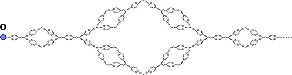

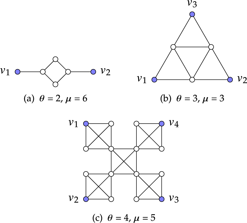
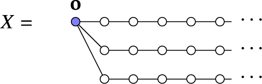
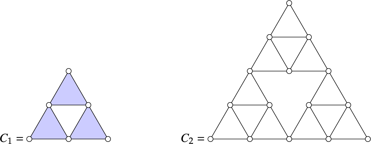


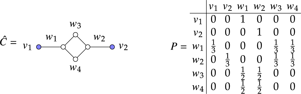

 Open access