


1 Introduction
Lithium-ion batteries (LIBs) are currently one of the most hopeful prospects for large-scale efficient storage of electricity for mobile devices from phones to cars. Crucial to their continued improved performance is to understand how novel materials might be effectively exploited in their design. Excellent reviews of the current status of such materials are given by [Reference Blomgren9, Reference Bruce, Scrosati and Tarascon12, Reference Choi, Chen, Freunberger, Ji, Sun, Amine, Yushin, Nazar, Cho and Bruce14]. Understanding how these materials affect macroscopic battery behaviour is greatly aided by good mathematical models of the transport processes within the battery.
The purpose of this paper is to serve as a guide to charge transport modelling in LIBs. Much of the work in this area is due to John Newman and his co-workers who, in a series of seminal publications [Reference Doyle, Fuller and Newman25, Reference Doyle, Newman, Gozdz, Schmutz and Tarascon26, Reference Fuller, Doyle and Newman40, Reference Ma, Doyle, Fuller, Doeff, De Jonghe and Newman63, Reference Newman68–Reference Newman, Thomas, Hafezi and Wheeler70, Reference Srinivasan and Newman92], introduced and applied models for these devices that account both for charge transport in the electrolyte as well as solid lithium ion diffusion in the active electrode materials and use Butler–Volmer reaction kinetics for lithium intercalation and de-intercalation on the electrode/electrolyte surface to couple these two processes together. While these models have been remarkably successful in describing the behaviour of real batteries, they are not easily extracted from the literature and, in addition, improvements in understanding of electrode materials have led to significant recent advances in the modelling of lithium transport in electrode particles that can be incorporated into this framework. This work aims to provide a relatively concise guide to the subject while at the same time highlighting some of the common modelling pitfalls. Alternative modelling approaches include lumped parameter equivalent circuit models, which are incapable of capturing the physical detail that the Newman model does. However, they are fast to compute with and so are often used on larger-scale systems, such as pouch cells which are fabricated by stacking many single cells on top of each other, where the primary goal may be to investigate the thermal behaviour of the system, see for example [Reference Plett75, Reference Troxler, Wu, Marinescu, Yufit, Patel, Marquis, Brandon and Offer97], or to develop a battery management system. At the opposite end of the scale, density functional theory is applied to study battery physics on the atomistic scale, but the computational costs are so high that the simulation of even a single battery cell is out of reach of the most powerful modern computers, see [Reference Dziedzic, Bhandari, Anton, Peng, Womack, Famili, Kramer and Skylaris28]. The charge transport models discussed here provide a useful compromise between capturing meaningful physics, but nevertheless being cheap enough to use on problems of engineering relevance.
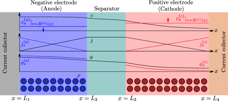
A typical LIB cell has three regions: (i) a porous negative electrode, (ii) a porous positive electrode and (iii) an electron-blocking separator (see Figure 1). Typically, the electrodes are comprised of particles, typically a few microns in size, of different (solid) active materials (AMs), that are capable of absorbing lithium into their structure and therefore act as lithium reservoirs. These particles are interspersed with an inert porous polymer binder material, combined with highly conducting carbon black, that acts to hold the electrode particles in place and form conducting links between electrode particles. The AM particle and polymer binder regions are permeated by a lithium electrolyte that serves to transport charge and lithium ions between the AMs of the two electrodes, with direct electrical contact between the negative and positive electrodes being prevented by the presence of the porous separator. On the interfaces between the electrode particles and the electrolyte (de-)intercalation reactions, in which lithium ion transfer between the electrolyte and the AM, take place. The AM of the positive electrode shows a greater affinity for lithium than that of the negative electrode so that in a charged cell there is a propensity for a current of positively charged lithium ions to flow from the negative to the positive electrode and thereby establishing a useful potential difference between the electrodes. The rates at which these (de-)intercalation reactions take place on the electrode–electrolyte interfaces are key to the electrical behaviour of the battery and are typically described by a Butler–Volmer relation which gives the interfacial current density, from AM to electrolyte, in terms of the potential jump between the AM and the electrolyte and the lithium concentrations in the AM and the electrolyte.
A sketch of a cross section of a typical device as well as the macroscopic variables and their domains of definition.
In addition to discussing transport models, we also propose a new formulation for the Butler–Volmer relation, for current flow between the AM and electrolyte, with the aim of ensuring a model that is able to simulate extreme cases, where classical formulations lead to physically unrealistic lithium distributions. More precisely, we address the issues of the limiting conditions in which the electrodes are close to being fully intercalated (or fully depleted) or in which the electrolyte concentration is very low.
LIBs are great examples of both multiscale and multiphysics systems. Accurately predicting the behaviour of commercial large format cells, which are used in consumer electronics and which are variously formed by layering many individual cells on top of each other (pouch cell) or winding one very large cell around a central core (cylindrical and prismatic cells), depends on having appropriate representations of the physics and chemistry at a range of smaller scales, including that of individual cells within a pack, individual electrodes within each cell, individual particles within electrodes and at the level of the atomic structure of the materials making up the particles. The behaviour at many of these lengthscales is dictated by a myriad of interacting phenomena including electrochemical ones, but also thermal and mechanical ones. The seminal models developed by Newman and his co-workers span the scales of individual electrodes particles up to individual cells and are largely focused on the electrochemical behaviour. Many authors including [Reference Franco38, Reference Ranom77, Reference Schmuck84] discuss the challenges associated with formulating mathematical models that couple phenomena occurring at vastly disparate lengthscales. There is also current impetus to experimentally characterise and develop new modelling approaches to better understand chemical structure within electrode materials [Reference Harris, Foster, Tessaro, Jiang, Yang, Wu, Protas and Goward44, Reference Kim, Johnson, Vaughey, Thackeray, Hackney, Yoon and Grey52], mechanical and thermal effects [Reference Oh, Siegel, Secondo, Kim, Samad, Qin, Anderson, Garikipati, Knobloch, Epureanu, Monroe and Stefanopoulou72], chemical degradation [Reference Birkl, Roberts, McTurk, Bruce and Howey7, Reference Monroe and Newman67, Reference Nishikawa, Mori, Nishida, Fukunaka and Rosso71, Reference Sethurajan, Foster, Richardson, Krachkovskiy, Bazak, Goward and Protas85, Reference Wang, Zeng, Hong, Xu, Yang, Wang, Duan, Tang and Jiang100], and to also develop battery management systems to optimally control batteries for use in electric vehicles [Reference Kim, Albertus, Cook, Monroe and Christensen53, Reference Lu, Han, Li, Hua and Ouyang62].
The outline of this work is as follows. In Section 2, we discuss charge transport models for the electrolyte. We begin, in Section 2.1, with the simplest description, dilute electrolyte theory and show that it cannot adequately describe electrolyte data at the typical concentrations encountered in real batteries. This motivates us to consider Newman’s moderately concentrated electrolyte theory [Reference Newman68, Reference Newman and Thomas-Alyea69] in Section 2.2, which forms the basis for much of the battery electrolyte modelling currently being undertaken and to show how this fits to real data for the common electrolyte LiPF
 $_6$
[Reference Valøen and Reimers98]. In Section 3, lithium transport within AM electrode particles is briefly reviewed, while in Section 3.1.2 a new formulation for the Butler–Volmer relation is proposed. In Section 4, the various strands of the battery chemistry, described in the previous sections, are brought together to formulate a macroscopic device-scale model for an entire cell. This is accomplished via homogenisation method set out in Section 4.2. In Section 5, we present a selection of solutions of the device-scale model for a common modern device configuration. Finally, in Section 6, we review the key insights of this work.
$_6$
[Reference Valøen and Reimers98]. In Section 3, lithium transport within AM electrode particles is briefly reviewed, while in Section 3.1.2 a new formulation for the Butler–Volmer relation is proposed. In Section 4, the various strands of the battery chemistry, described in the previous sections, are brought together to formulate a macroscopic device-scale model for an entire cell. This is accomplished via homogenisation method set out in Section 4.2. In Section 5, we present a selection of solutions of the device-scale model for a common modern device configuration. Finally, in Section 6, we review the key insights of this work.
2 Modelling the electrolyte
Here we begin, in Section 2.1, by considering the theory of very dilute electrolytes, often termed Poisson–Nernst–Planck (PNP) theory. Because the theory is commonly encountered in modelling semiconductors and is relatively straightforward and physically appealing, it is useful to highlight some of the peculiarities associated with charge transport modelling in batteries. These include charge neutrality, the use of electrochemical potentials and the measurement of the electric potential with respect to a lithium reference electrode. However, the price of simplicity is that dilute theory does not describe battery electrolyte behaviour particularly well. Many of these limitations are overcome in Newman’s theory of moderately concentrated electrolytes, which we review in Section 2.2. This theory is considerably more involved than the dilute theory and in practice requires that various functions be fitted to data directly measured from the electrolyte under consideration. However, within these limitations, it does provide a good description of most electrolytes formed by dissolution of a salt in a solvent. We also hope that by introducing the peculiarities of notation associated with battery electrolyte modelling in the context of the simpler dilute theory, it will make it easier for the reader to follow the more complex moderately concentrated theory.
2.1 Dilute electrolytes
We consider an electrolyte composed of a solvent, a negative ion with molar concentration
 $c_n$
and charge
$c_n$
and charge
 $z_n e$
, and a positive ion with molar concentration
$z_n e$
, and a positive ion with molar concentration
 $c_p$
and charge
$c_p$
and charge
 $z_pe$
(where e is the elementary charge, and
$z_pe$
(where e is the elementary charge, and
 $z_n$
and
$z_n$
and
 $z_p$
are integers accounting for the charge state). This general binary electrolyte can be easily studied but because the purpose of this section is to give a simple introduction in the rest of this article, we focus on a 1:1 electrolyte with a generic negative ion and a positive lithium ion Li
$z_p$
are integers accounting for the charge state). This general binary electrolyte can be easily studied but because the purpose of this section is to give a simple introduction in the rest of this article, we focus on a 1:1 electrolyte with a generic negative ion and a positive lithium ion Li
 $^+$
, so that
$^+$
, so that
 $z_n=-1$
and
$z_n=-1$
and
 $z_p=1$
.
$z_p=1$
.
Because of the long timescales over which batteries are typically charged and discharged, it is entirely reasonable to neglect magnetic effects and assume that the electric field
 ${\textbf{E}}$
is irrotational (i.e.
${\textbf{E}}$
is irrotational (i.e.
 $\nabla \times \textbf{E}=\textbf{0}$
) so that it can be written in terms of an electric potential
$\nabla \times \textbf{E}=\textbf{0}$
) so that it can be written in terms of an electric potential
 $\phi$
, via the relation:
$\phi$
, via the relation:
 \begin{eqnarray}\textbf{E}=-\nabla \phi.\end{eqnarray}
Considering the charge within the system then gives Poisson’s equation:
 \begin{eqnarray}\nabla \cdot (\varepsilon \nabla \phi ) = F (c_n-c_p),\end{eqnarray}
where F is Faraday’s constant and
 $\varepsilon$
is the permittivity of the electrolyte.
$\varepsilon$
is the permittivity of the electrolyte.
Since the ions in battery electrolytes do not react with each other or with the solvent, conservation of the two ion species implies that
 \begin{eqnarray}\frac{\partial c_n}{\partial t} + \nabla \cdot \textbf{q}_n=0, \quad \mbox{and}\quad \frac{\partial c_p}{\partial t} + \nabla \cdot \textbf{q}_p=0,\end{eqnarray}
where
 $\textbf{q}_p$
and
$\textbf{q}_p$
and
 $\textbf{q}_n$
are the fluxes of positive and negative ions, respectively. We can also write this using
$\textbf{q}_n$
are the fluxes of positive and negative ions, respectively. We can also write this using
 $\textbf{q}_p=c_p \textbf{v}_p$
and
$\textbf{q}_p=c_p \textbf{v}_p$
and
 $q_n = c_n \textbf{v}_n$
where
$q_n = c_n \textbf{v}_n$
where
 $\textbf{v}_p$
and
$\textbf{v}_p$
and
 $\textbf{v}_n$
are the average velocities of the respective species. In the dilute limit, the electrolyte solvent is assumed to be stationary and the ions to move in response to thermal diffusion and electric fields; interactions between ions are neglected. The component of the average velocity of a lithium ion due to the electric field,
$\textbf{v}_n$
are the average velocities of the respective species. In the dilute limit, the electrolyte solvent is assumed to be stationary and the ions to move in response to thermal diffusion and electric fields; interactions between ions are neglected. The component of the average velocity of a lithium ion due to the electric field,
 $\textbf{v}_{ep}$
, is given by balancing the force
$\textbf{v}_{ep}$
, is given by balancing the force
 $e \textbf{E}$
, exerted on it by the electric field, with the viscous drag force
$e \textbf{E}$
, exerted on it by the electric field, with the viscous drag force
 $ \textbf{v}_{ep}/M_p$
, exerted on it by the solvent (here
$ \textbf{v}_{ep}/M_p$
, exerted on it by the solvent (here
 $M_p$
is the mobility of the lithium ion). Thus, the advective lithium ion velocity due to the electric field is
$M_p$
is the mobility of the lithium ion). Thus, the advective lithium ion velocity due to the electric field is
 $\textbf{v}_{ep}=-e M_p \nabla \phi$
and in a similar manner the average negative ion velocity can be shown to be
$\textbf{v}_{ep}=-e M_p \nabla \phi$
and in a similar manner the average negative ion velocity can be shown to be
 $\textbf{v}_{en}=e M_n \nabla \phi$
. In addition to the advective fluxes (
$\textbf{v}_{en}=e M_n \nabla \phi$
. In addition to the advective fluxes (
 $c_p \textbf{v}_{ep}$
and
$c_p \textbf{v}_{ep}$
and
 $c_n \textbf{v}_{en}$
), both ion species diffuse, in response to random thermal excitations. This gives rise to Fickian fluxes (for positive and negative ions) of size
$c_n \textbf{v}_{en}$
), both ion species diffuse, in response to random thermal excitations. This gives rise to Fickian fluxes (for positive and negative ions) of size
 $-D_p \nabla c_p$
and
$-D_p \nabla c_p$
and
 $-D_n \nabla c_n$
, respectively, where
$-D_n \nabla c_n$
, respectively, where
 $D_p$
and
$D_p$
and
 $D_n$
are the respective diffusion coefficients. To highlight the difference between these diffusion coefficients and those used in the Stefan–Maxwell theory that we will review in Section 2.2, let us point out that
$D_n$
are the respective diffusion coefficients. To highlight the difference between these diffusion coefficients and those used in the Stefan–Maxwell theory that we will review in Section 2.2, let us point out that
 $D_p$
(respectively,
$D_p$
(respectively,
 $D_n$
) is the diffusion coefficient for positive (respectivley, negative) ions in a mixture of solvent and negative (respectively, positive) ions. The total ion fluxes,
$D_n$
) is the diffusion coefficient for positive (respectivley, negative) ions in a mixture of solvent and negative (respectively, positive) ions. The total ion fluxes,
 $\textbf{q}_n$
and
$\textbf{q}_n$
and
 $\textbf{q}_p$
, are obtained by summing their advective and diffusive components, so that
$\textbf{q}_p$
, are obtained by summing their advective and diffusive components, so that
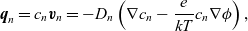 \begin{align} \textbf{q}_n = c_n \textbf{v}_n = -D_n \left( \nabla c_n - \frac{e}{k T} c_n \nabla \phi \right), \end{align}
 \begin{eqnarray}\textbf{q}_p = c_p \textbf{v}_p = -D_p\left( \nabla c_p + \frac{e}{k T} c_p \nabla \phi\right).\end{eqnarray}
Here, we have substituted for ion mobilities in terms of the diffusion coefficients by using the Einstein relations
 $M_p=D_p/kT$
and
$M_p=D_p/kT$
and
 $M_n=D_n/kT$
(where k is Boltzmann’s constant). Since this theory is applied in a chemical setting, it is more usual to write these equations in terms of Faraday’s constant F and the universal gas constant R which, on noting that
$M_n=D_n/kT$
(where k is Boltzmann’s constant). Since this theory is applied in a chemical setting, it is more usual to write these equations in terms of Faraday’s constant F and the universal gas constant R which, on noting that
 $e/k=F/R$
, leads to the alternative expressions:
$e/k=F/R$
, leads to the alternative expressions:
 \begin{eqnarray}\textbf{q}_n= -D_n \left( \nabla c_n - \frac{F}{R T} c_n \nabla \phi\right), \quad \mbox{and} \quad \textbf{q}_p=-D_p\left( \nabla c_p + \frac{F}{R T}c_p \nabla \phi \right).\end{eqnarray}
The equations governing the three variables,
 $c_n$
,
$c_n$
,
 $c_p$
and
$c_p$
and
 $\phi$
, are thus (2.2), (2.3) and (2.5).
$\phi$
, are thus (2.2), (2.3) and (2.5).
2.1.1 Double layers and charge neutrality
It has long been recognised that (see e.g. [Reference Newman and Thomas-Alyea69]), at the concentrations typically encountered in practical electrolytes, there is almost exact charge neutrality. This implies that there is a balance between the concentrations of positive and negative charges, throughout the vast majority of the electrolyte. The exception to this rule is in the so-called double layers which lie along the boundaries of the electrolyte region and are typically extremely thin, with widths less than a few nanometres. This observation can be justified mathematically by non-dimensionalising equations (2.2), (2.3) and (2.5) and conducting a boundary layer analysis in terms of the small dimensionless parameter which measures the ratio of the Debye length (i.e. the typical width of a double layer) to the typical dimension of the electrolyte.Footnote
1
The result of such an analysis (see, e.g. [Reference Richardson78]) is that, with the exception of the double layers,
 $c_n$
must be almost exactly equal to
$c_n$
must be almost exactly equal to
 $c_p$
. The physical meaning of this fact is that the attraction between charges is very strong compared to any space charge that the electric field may create. Therefore, a very good approximation to (2.2) is
$c_p$
. The physical meaning of this fact is that the attraction between charges is very strong compared to any space charge that the electric field may create. Therefore, a very good approximation to (2.2) is
 \begin{eqnarray}0= c_n - c_p,\end{eqnarray}
which is usually called the charge neutrality condition. As we shall discuss later, because (2.6) has neglected the derivatives that were in (2.2), the model needs fewer boundary conditions at the edges of the electrolyte (i.e. only two boundary conditions are required on the electrolyte ‘surface’ rather than the three needed for the full system).
2.1.2 The approximate equations
In line with the discussion above, we introduce a single concentration c by taking
 \begin{eqnarray}c_n=c_p=c, \end{eqnarray}
and substitute this into (2.3) and (2.5) to obtain the approximate charge-neutral equations:
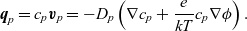
 \begin{eqnarray}\frac{\partial c}{\partial t} + \nabla \cdot \textbf{q}_n=0, \quad \mbox{and} \quad \textbf{q}_n= -D_n \left( \nabla c - \frac{F}{R T} c \nabla \phi \right), \end{eqnarray}
 \begin{eqnarray}\frac{\partial c}{\partial t} + \nabla \cdot \textbf{q}_p=0, \quad \mbox{and} \quad \textbf{q}_p=-D_p\left( \nabla c + \frac{F}{R T}c \nabla \phi \right). \end{eqnarray}
A common approach to studying this problem is to assume that the ionic diffusivities
 $D_n$
and
$D_n$
and
 $D_p$
are constant and rewrite the system by adding the former equation in (2.8a) multiplied by
$D_p$
are constant and rewrite the system by adding the former equation in (2.8a) multiplied by
 $D_p$
to the former equation in (2.8b) multiplied by
$D_p$
to the former equation in (2.8b) multiplied by
 $D_n$
. On substituting for
$D_n$
. On substituting for
 $\textbf{q}_n$
and
$\textbf{q}_n$
and
 $\textbf{q}_p$
, this yields a diffusion equation for c, of the form:
$\textbf{q}_p$
, this yields a diffusion equation for c, of the form:
 \begin{eqnarray}\frac{\partial c}{\partial t} - {D_{\rm eff}}\nabla^2 c = 0\quad \mbox{with} \quad {D_{\rm eff}}=2\frac{D_n D_p}{D_n+D_p},\end{eqnarray}
where
 ${D_{\rm eff}}$
is termed the effective ionic diffusivity.
${D_{\rm eff}}$
is termed the effective ionic diffusivity.
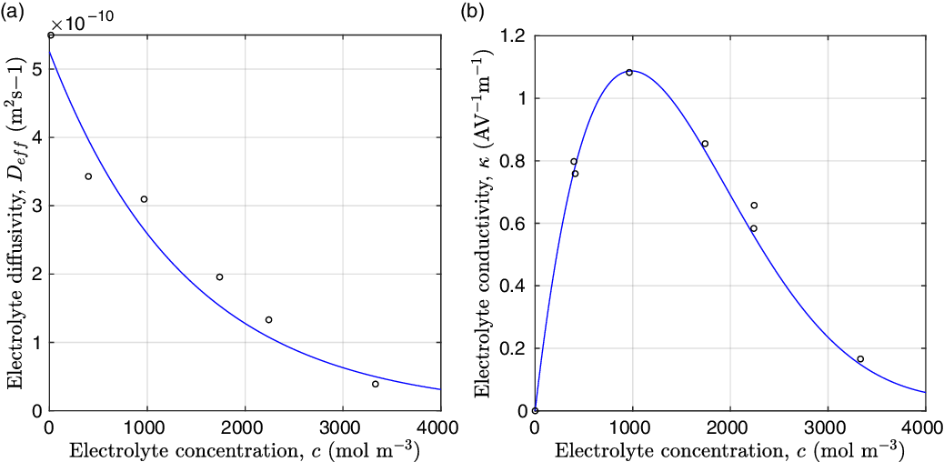
(a) Diffusion coefficient
 ${D_{\rm eff}}$
for LiPF
${D_{\rm eff}}$
for LiPF
 $_{6}$
in 1:1 EC:DMC at
$_{6}$
in 1:1 EC:DMC at
 $T=293$
K as a function of concentration and (b) electrolyte conductivity
$T=293$
K as a function of concentration and (b) electrolyte conductivity
 $\kappa$
for the same electrolyte. Lines represent the fit to to the experimental data (circles) taken from [Reference Valøen and Reimers98]. The fitted functions for the diffusivity and conductivity are given by
$\kappa$
for the same electrolyte. Lines represent the fit to to the experimental data (circles) taken from [Reference Valøen and Reimers98]. The fitted functions for the diffusivity and conductivity are given by
 ${D_{\rm eff}}(c)=5.3\times 10^{-10} \exp(-7.1\times 10^{-4}c)$
and
${D_{\rm eff}}(c)=5.3\times 10^{-10} \exp(-7.1\times 10^{-4}c)$
and
 $\kappa(c)=10^{-4} c (5.2-0.002c+2.3\times10^{-7}c^2)^2$
, respectively. We note that an exponential fitting function is ubiquitous throughout the literature and can be found in numerous other sources, for example, [Reference Stewart and Newman93].
$\kappa(c)=10^{-4} c (5.2-0.002c+2.3\times10^{-7}c^2)^2$
, respectively. We note that an exponential fitting function is ubiquitous throughout the literature and can be found in numerous other sources, for example, [Reference Stewart and Newman93].
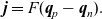
Useful physical insight can be found using an alternative formulation of (2.8a) and (2.8b) by introducing the electric current density,
 $\textbf{j}$
, defined in terms of the ion fluxes by:
$\textbf{j}$
, defined in terms of the ion fluxes by:
 \begin{eqnarray}\textbf{j}=F(\textbf{q}_p-\textbf{q}_n).\end{eqnarray}
Using this concept, a version of Ohm’s law may be obtained by subtracting (2.8a b) from (2.8a b), while a charge conservation equation may be found by subtracting (2.8aa) from (2.8b a). These may be written in the form:
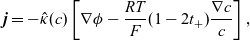 \begin{eqnarray}{\textbf{j}=-\hat{\kappa}(c) \left[\nabla \phi - \frac{RT}{F} (1- 2t_+) \frac{\nabla c}{c} \right],}\end{eqnarray}
 \begin{eqnarray}{\nabla \cdot \textbf{j}=0,}\end{eqnarray}
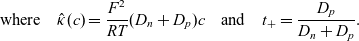 \begin{eqnarray} \mbox{where} \quad \hat{\kappa}(c)=\frac{F^2}{R T}(D_n+D_p) c \quad \mbox{and} \quad t_+ =\frac{D_p}{D_n+D_p}.\end{eqnarray}
Here
 $t_+$
is referred to as the transference number and
$t_+$
is referred to as the transference number and
 $\hat{\kappa}(c)$
is referred to as the electrical conductivity of the electrolyte (c.f. the standard form of Ohm’s law is
$\hat{\kappa}(c)$
is referred to as the electrical conductivity of the electrolyte (c.f. the standard form of Ohm’s law is
 $\textbf{j}=-\kappa \nabla\phi$
). We use the notation
$\textbf{j}=-\kappa \nabla\phi$
). We use the notation
 $\hat{\kappa}$
to distinguish the electrical conductivity in the dilute limit from the same quantity in moderately concentrated theory, see (2.43). The alternative formulation of (2.8a) and (2.8b) mentioned above is then (2.9), (2.11a) and (2.11b).
$\hat{\kappa}$
to distinguish the electrical conductivity in the dilute limit from the same quantity in moderately concentrated theory, see (2.43). The alternative formulation of (2.8a) and (2.8b) mentioned above is then (2.9), (2.11a) and (2.11b).
Assuming that the ionic diffusivities
 $D_n$
and
$D_n$
and
 $D_p$
are constant implies (i) that transference number
$D_p$
are constant implies (i) that transference number
 $t_+$
is constant, (ii) the effective ionic diffusivity
$t_+$
is constant, (ii) the effective ionic diffusivity
 ${D_{\rm eff}}$
is constant and (iii) electrolyte conductivity
${D_{\rm eff}}$
is constant and (iii) electrolyte conductivity
 $\kappa$
grows linearly with electrolyte concentration c. All three of these quantities are readily measured experimentally for real electrolytes. For most electrolytes, the transference number is usually found to remain close to a constant (with the exception of some polymer electrolytes e.g. [Reference Doeff, Edman, Sloop, Kerr and De Jonghe24, Reference Fauteux32]), electrolyte diffusivity usually decreases relatively weakly with concentration, except at very dilute concentrations, but the growth of electrical conductivity with concentration is far from linear. Examples of the experimentally measured concentration dependence of
$\kappa$
grows linearly with electrolyte concentration c. All three of these quantities are readily measured experimentally for real electrolytes. For most electrolytes, the transference number is usually found to remain close to a constant (with the exception of some polymer electrolytes e.g. [Reference Doeff, Edman, Sloop, Kerr and De Jonghe24, Reference Fauteux32]), electrolyte diffusivity usually decreases relatively weakly with concentration, except at very dilute concentrations, but the growth of electrical conductivity with concentration is far from linear. Examples of the experimentally measured concentration dependence of
 ${D_{\rm eff}}$
and
${D_{\rm eff}}$
and
 $\kappa$
(from [Reference Valøen and Reimers98]) are plotted in Figure 2 for the battery electrolyte LiPF
$\kappa$
(from [Reference Valøen and Reimers98]) are plotted in Figure 2 for the battery electrolyte LiPF
 $_6$
. Notably at the typical concentrations used in batteries (roughly 1 molar for LiPF
$_6$
. Notably at the typical concentrations used in batteries (roughly 1 molar for LiPF
 $_6$
), electrical conductivity is nearly constant and often lies close to its maximum value and is thus not well approximated by the linear expression in (2.11c). The explanation given for this poor fit is usually that even at relatively dilute concentrations, there is a significant drag between ions of opposite charge. The reason for this is that two ions of opposite charge that lie close to each other experience a significant electrostatic attraction that negates, to a large extent, the effects of the global electric field which is trying to drive the ions in opposite directions. This observation has motivated Newman [Reference Newman and Thomas-Alyea69] to use Stefan–Maxwell theory for a multi-component solution to describe the charge transport behaviour of electrolytes. A summary of the modelling assumptions made in this theory is given in Section 2.2.
$_6$
), electrical conductivity is nearly constant and often lies close to its maximum value and is thus not well approximated by the linear expression in (2.11c). The explanation given for this poor fit is usually that even at relatively dilute concentrations, there is a significant drag between ions of opposite charge. The reason for this is that two ions of opposite charge that lie close to each other experience a significant electrostatic attraction that negates, to a large extent, the effects of the global electric field which is trying to drive the ions in opposite directions. This observation has motivated Newman [Reference Newman and Thomas-Alyea69] to use Stefan–Maxwell theory for a multi-component solution to describe the charge transport behaviour of electrolytes. A summary of the modelling assumptions made in this theory is given in Section 2.2.
2.1.3 The dilute theory in terms of electrochemical potentials
The dilute model (2.8a)–(2.8b) can also be written in terms of the electrochemical potentials,
 $\bar{\mu}_n$
and
$\bar{\mu}_n$
and
 $\bar{\mu}_p$
, of negative and positive ions, respectively. This is the preferred notation for the ion conservation equations in the electrochemical literature. For an electrolyte that is formed by ideal salt solution, the electrochemical potentials are given by:
$\bar{\mu}_p$
, of negative and positive ions, respectively. This is the preferred notation for the ion conservation equations in the electrochemical literature. For an electrolyte that is formed by ideal salt solution, the electrochemical potentials are given by:
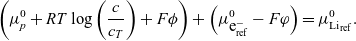
 \begin{eqnarray}\bar{\mu}_n=\mu_n^0+ RT \log \left( \frac{c}{c_T} \right) - F \phi, \qquad \bar{\mu}_p=\mu_p^0+ RT \log \left( \frac{c}{c_T} \right) +F \phi,\end{eqnarray}
where
 $c_T$
is the total molar concentration of the electrolyte and, for a dilute solution, is approximately equal to the solvent concentration. The first term on the right-hand sides of both expressions in (2.12) is the standard state potential (per mole of the species), while the second is the entropy of mixing (per mole of the species) and the final term is the electrostatic potential (per mole of the species). Using this notation, the conservation equations (2.8a) and (2.8b) can be written in the form:
$c_T$
is the total molar concentration of the electrolyte and, for a dilute solution, is approximately equal to the solvent concentration. The first term on the right-hand sides of both expressions in (2.12) is the standard state potential (per mole of the species), while the second is the entropy of mixing (per mole of the species) and the final term is the electrostatic potential (per mole of the species). Using this notation, the conservation equations (2.8a) and (2.8b) can be written in the form:
 \begin{eqnarray}\frac{\partial c}{\partial t} + \nabla \cdot (c \textbf{v}_n)=0, \quad \mbox{and} \quad\textbf{v}_n= -\frac{D_n}{RT} \nabla \bar{\mu}_n,\end{eqnarray}
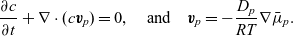 \begin{eqnarray}\frac{\partial c}{\partial t} + \nabla \cdot (c \textbf{v}_p)=0, \quad \mbox{and} \quad\textbf{v}_p=-\frac{D_p}{RT} \nabla \bar{\mu}_p.\end{eqnarray}
Here the average velocities of the two species,
 $\textbf{v}_n$
and
$\textbf{v}_n$
and
 $\textbf{v}_p$
, are obtained by multiplying the gradient of the electrochemical potentials by the species mobilities,
$\textbf{v}_p$
, are obtained by multiplying the gradient of the electrochemical potentials by the species mobilities,
 ${D_n}/{RT}$
and
${D_n}/{RT}$
and
 ${D_p}/{RT}$
. This formalism extends to non-ideal salt solutions and to multicomponent systems. In Section 2.2, this approach of using electrochemical potentials is extended to moderately concentrated electrolytes.
${D_p}/{RT}$
. This formalism extends to non-ideal salt solutions and to multicomponent systems. In Section 2.2, this approach of using electrochemical potentials is extended to moderately concentrated electrolytes.
2.1.4 The potential measured with respect to a lithium electrode
The dilute theory as formulated above is at odds with the electrolyte theory used by [Reference Newman and Thomas-Alyea69]; here, the factor in front of the concentration gradient in (2.11a), the constitutive law for the current, is
 $2({RT}/{F}) (1- t_+)$
rather than
$2({RT}/{F}) (1- t_+)$
rather than
 $({RT}/{F}) (1- 2 t_+)$
as above. As pointed out in [Reference Ramos76], this has generated some confusion in the literature. The explanation for this discrepancy (as initially demonstrated by [Reference Ranom77] and subsequently in [Reference Bizeray, Howey and Monroe8]) is that the theory in [Reference Newman and Thomas-Alyea69] is formulated in terms of
$({RT}/{F}) (1- 2 t_+)$
as above. As pointed out in [Reference Ramos76], this has generated some confusion in the literature. The explanation for this discrepancy (as initially demonstrated by [Reference Ranom77] and subsequently in [Reference Bizeray, Howey and Monroe8]) is that the theory in [Reference Newman and Thomas-Alyea69] is formulated in terms of
 $\varphi$
, the electric potential measured with respect to a reference lithium electrode, rather than
$\varphi$
, the electric potential measured with respect to a reference lithium electrode, rather than
 $\phi$
, the true electric potential. In electrochemical applications, the potential in an electrolyte is typically measured by inserting a reference electrode of a pure compound. The potential measured depends on the composition of the reference electrode through its chemical potential. Since in lithium battery applications, the reference electrode used is nearly always made of lithium, and since much of the data used to calibrate battery models is collected using a lithium reference electrode, it makes sense to use the potential measured with respect to a lithium electrode. Note that
$\phi$
, the true electric potential. In electrochemical applications, the potential in an electrolyte is typically measured by inserting a reference electrode of a pure compound. The potential measured depends on the composition of the reference electrode through its chemical potential. Since in lithium battery applications, the reference electrode used is nearly always made of lithium, and since much of the data used to calibrate battery models is collected using a lithium reference electrode, it makes sense to use the potential measured with respect to a lithium electrode. Note that
 $\phi$
, the true electric potential, is not a readily measured quantity. In order to switch between
$\phi$
, the true electric potential, is not a readily measured quantity. In order to switch between
 $\varphi$
and
$\varphi$
and
 $\phi$
, we recall that there is a reversible reaction that occurs on the surface of the electrode between intercalated lithium in the electrode and lithium ions in the electrolyte, given by:
$\phi$
, we recall that there is a reversible reaction that occurs on the surface of the electrode between intercalated lithium in the electrode and lithium ions in the electrolyte, given by:
 \begin{eqnarray}\mbox{Li}^+_{(l)} + \mbox{e}^-_{(\rm ref)} \leftrightharpoons \mbox{Li}_{(\rm ref)}, \end{eqnarray}
where, since the lithium atom in the reference electrode is neutral, its electrochemical potential is equal to its chemical potential
 $\mbox{Li}_{(\rm ref)}$
. Here, the subscript (l) denotes a reactant within the electrolyte and
$\mbox{Li}_{(\rm ref)}$
. Here, the subscript (l) denotes a reactant within the electrolyte and
 $(\rm ref)$
one within the reference electrode. Typically, the current flow into a reference electrode can be assumed to be sufficiently small that this reaction is in quasi-equilibrium. It follows that the electrochemical potentials of compounds on both sides of this equation are equal, that is
$(\rm ref)$
one within the reference electrode. Typically, the current flow into a reference electrode can be assumed to be sufficiently small that this reaction is in quasi-equilibrium. It follows that the electrochemical potentials of compounds on both sides of this equation are equal, that is
 \begin{eqnarray}\bar{\mu}_{p}+ \bar{\mu}_{\mbox{e}^-_{\rm ref}}=\mu_{{Li}_{\rm ref}}. \end{eqnarray}
Since the potential within the lithium electrode is
 $\varphi$
the electrochemical potential of the electrons can be expressed as
$\varphi$
the electrochemical potential of the electrons can be expressed as
 $\bar{\mu}_{\mbox{e}^-_{\rm ref}}=\mu^0_{\mbox{e}^-_{\rm ref}}-F \varphi$
, where
$\bar{\mu}_{\mbox{e}^-_{\rm ref}}=\mu^0_{\mbox{e}^-_{\rm ref}}-F \varphi$
, where
 $\mu^0_{\mbox{e}^-_{\rm ref}}$
is the work function of the lithium electrode. Furthermore, the lithium concentration within the electrode does not change, so that
$\mu^0_{\mbox{e}^-_{\rm ref}}$
is the work function of the lithium electrode. Furthermore, the lithium concentration within the electrode does not change, so that
 $\mu_{{Li}_{\rm ref}}$
is fixed, and equal to
$\mu_{{Li}_{\rm ref}}$
is fixed, and equal to
 $\mu^0_{{Li}_{\rm ref}}$
. The electrochemical balance (2.15) thus implies that
$\mu^0_{{Li}_{\rm ref}}$
. The electrochemical balance (2.15) thus implies that
 \begin{eqnarray*}\left(\mu_p^0+ RT \log \left( \frac{c}{c_T} \right)+F \phi \right) +\left( \mu^0_{\mbox{e}^-_{\rm ref}} - F \varphi\right)=\mu^0_{{Li}_{\rm ref}}.\end{eqnarray*}
This leads to the following expression for the electric potential
 $\phi$
in terms of
$\phi$
in terms of
 $\varphi$
:
$\varphi$
:
 \begin{eqnarray}\begin{array}{l}\displaystyle \phi=\varphi +V^0_*- \frac{1}{F} \left(\mu_p^0+ RT\log \left( \frac{c}{c_T} \right)\right),\\\displaystyle \mbox{where} \quad V^0_*=\frac{1}{F} (\mu^0_{{Li}_{\rm ref}}-\mu^0_{\mbox{e}^-_{\rm ref}}).\end{array}\end{eqnarray}
Notably, with this new notation, the electrochemical potential of the two ion species now read
 \begin{eqnarray}\bar{\mu}_p=F (\varphi+V^0_*), \qquad \bar{\mu}_n=2 \mu_e(c) - F (\varphi+V^0_*)\end{eqnarray}
where
 $\mu_e(c)$
, the chemical potential of the electrolyte, is defined such that
$\mu_e(c)$
, the chemical potential of the electrolyte, is defined such that
 \begin{eqnarray}\mu_e(c) =\frac{\mu_n+\mu_p}{2}, \quad \mbox{or equivalently} \quad \mu_e(c) =\frac{\mu^0_n+\mu^0_p}{2}+RT \log \left( \frac{c}{c_T} \right).\end{eqnarray}
Using (2.16) to substitute for
 $\phi$
in (2.11a) yields the electrolytic version of Ohm’s law found in the Newman theory:
$\phi$
in (2.11a) yields the electrolytic version of Ohm’s law found in the Newman theory:
 \begin{eqnarray}\textbf{j}=-\hat{\kappa}(c) \left[\nabla \varphi -2 \frac{RT}{F} (1- {t_+}) \frac{\nabla c}{c} \right].\end{eqnarray}
The effect of the difference in the two different potentials is now readily seen by comparing (2.19) with (2.11a). Therefore (2.19), together with (2.9) and (2.11b) is a system of equations equivalent to the charge-neutral equations (2.8a) and (2.8b).
2.2 Moderately concentrated electrolytes
Motivated by the confusion in the literature highlighted in [Reference Ramos76], this section reviews, in detail, a commonly used model for moderately concentrated electrolytes, presented in [Reference Newman and Thomas-Alyea69], which is applicable to most electrolytes consisting of a salt dissolved in a solvent but not to ionic liquids. In most practical battery systems, ion transport takes place through electrolytic solutions which do not behave as ideal dilute materials as demonstrated primarily by the concentration dependence of their conductivity, see [Reference Valøen and Reimers98], but also by activity coefficient measurements, for example, those in [Reference Samson, Lemaire, Marchand and Beaudoin82]. In order to capture this non-ideal behaviour, it is necessary to consider not only ion–solvent interactions (as is done in the PNP theory of ideal electrolytes as covered in Section 2.1) but also interactions between the ionic species. Inter-ionic interactions are significant, in even relatively dilute solutions, because the local attraction between oppositely charged ions result in a propensity for ions of opposite charge to lie close to each other, which reduces their mobility in an electric field. This, in turn, reduces the ionic conductivity, see [Reference Samson, Lemaire, Marchand and Beaudoin82]. Models of batteries that use electrolytes in this moderately concentrated regime have been pioneered and applied successfully to a variety of systems. For example, see the series of seminal works by John Newman and his co-workers: [Reference Doyle, Fuller and Newman25, Reference Doyle, Newman, Gozdz, Schmutz and Tarascon26, Reference Newman68–Reference Newman, Thomas, Hafezi and Wheeler70, Reference Srinivasan and Newman92].
The electrolyte theory reviewed below is based on the Stefan–Maxwell equations (see, for example, [Reference Bird, Stewart and Lightfoot6]), which describe transport in a mixture (including diffusion) in terms of the drag coefficients between its various components.
2.2.1 Stefan–Maxwell equations
We start by briefly considering the general case in which the electrolyte is comprised of N (ionic and solvent) species. Newman and Thomas-Alyea [Reference Newman and Thomas-Alyea69] uses the Stefan–Maxwell equations as the foundation of concentrated electrolyte theory. These relate the drag force acting on a component in a mixture to its relative velocity with the other components. It is by balancing these drag forces with gradients of electrochemical potential of a species and gradients in the fluid pressure that we obtain the average velocity of each species and in turn its flux. This combined with conservation laws for each species form the equations of moderately concentrated electrolyte theory. We note that other mechanisms in addition to the interspecies drag, electrochemical potential and pressure forces can also cause mass transfer and we briefly mention these without detailed dicussion.
In order to derive the force acting on each component of the mixture as a consequence of the pressure gradient, it is neccessary first to obtain an equation of state that relates the concentrations of the N species forming the mixture. According to [Reference Liu and Monroe61] for most electrolytes, it is usually a good approximation to assume that each species has constant molar volume. This is equivalent to the assumption that the volume occupied by one mole of a given species remains fixed whatever the composition of the mixture. On denoting the molar volume of the i’th species by
 $V_i$
, we obtain the following equation of state relating the molar concentrations:
$V_i$
, we obtain the following equation of state relating the molar concentrations:
 \begin{eqnarray}\sum_{i=1}^N V_i c_i=1. \end{eqnarray}
As we shall see, this relation allows us to write down the force on a species arising from the pressure gradient in the mixture. We note that electrolytes may have mechanical properties, such as acting as a viscous fluid or an elastic solid, which can create additional forces. We do not consider these but they can contribute significantly in certain situations.
The mutual friction force between species i and j is assumed to be proportional to the friction forces arising from velocity differences between the species. Furthermore, this force is proportional to the mole fraction,
 $\chi_k$
, of each species (see [Reference Bothe11]) as defined by:
$\chi_k$
, of each species (see [Reference Bothe11]) as defined by:
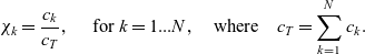 \begin{eqnarray}\chi_k=\frac{c_k}{c_T}, \quad\hbox{ for } k=1...N, \quad \mbox{where} \quad c_T=\sum_{k=1}^N c_k.\end{eqnarray}
Here,
 $c_k$
is the molar concentrations of species k and
$c_k$
is the molar concentrations of species k and
 $c_T$
is the total molar concentration of all species in the solution. The Stefan–Maxwell equations give a relation between
$c_T$
is the total molar concentration of all species in the solution. The Stefan–Maxwell equations give a relation between
 $\;\;{\hat{\textbf{d}}}_i$
, the drag force exerted on species i, per unit volume of mixture, and the velocities of the various species. In light of the above comments the drag force on the i’th species (per mole unit volume) is taken to depend linearly on the velocity differences between species, and modelled (see [Reference Bothe11]) by the expression:
$\;\;{\hat{\textbf{d}}}_i$
, the drag force exerted on species i, per unit volume of mixture, and the velocities of the various species. In light of the above comments the drag force on the i’th species (per mole unit volume) is taken to depend linearly on the velocity differences between species, and modelled (see [Reference Bothe11]) by the expression:
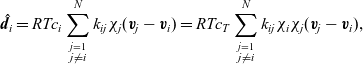 \begin{eqnarray}\;\;\hat{\textbf{d}}_i=RT c_i \sum_{\stackrel{j=1}{j \neq i}}^N k_{ij}\chi_j (\textbf{v}_j-\textbf{v}_i)=RT c_T \sum_{\stackrel{j=1}{j \neq i}}^N k_{ij} \chi_i\chi_j (\textbf{v}_j-\textbf{v}_i),\end{eqnarray}
where
 $\textbf{v}_k$
is the velocity of species k and
$\textbf{v}_k$
is the velocity of species k and
 $RT k_{ij}$
is the drag coefficient on one mole of species i moving through pure species j. Note that
$RT k_{ij}$
is the drag coefficient on one mole of species i moving through pure species j. Note that
 $k_{ij}$
is symmetric (i.e.
$k_{ij}$
is symmetric (i.e.
 $k_{ij}=k_{ji}$
) because the drag exerted on species i by species j is equal and opposite to that exerted on species j by species i. Here the Maxwell–Stefan inter-species diffusivity is related to
$k_{ij}=k_{ji}$
) because the drag exerted on species i by species j is equal and opposite to that exerted on species j by species i. Here the Maxwell–Stefan inter-species diffusivity is related to
 $k_{ij}$
by the Einstein relation so that
$k_{ij}$
by the Einstein relation so that
 $D_{ij}=1/k_{ij}$
.
$D_{ij}=1/k_{ij}$
.
The drag force,
 $\hat{\textbf{d}}_i$
, is balanced by motive forces (per unit volume) down gradients in the electrochemical potential
$\hat{\textbf{d}}_i$
, is balanced by motive forces (per unit volume) down gradients in the electrochemical potential
 $\bar{\mu}_i$
and down gradients in the pressure p:
$\bar{\mu}_i$
and down gradients in the pressure p:
 \begin{eqnarray}\hat{\textbf{d}}_i-c_i \nabla\bar{\mu}_i - V_i c_i \nabla p =\textbf{0}, \quad\hbox{ for } k=1...N.\end{eqnarray}
Here, the electrochemical potentials
 $\bar{\mu}_i$
may be rewritten in terms of the chemical potentials
$\bar{\mu}_i$
may be rewritten in terms of the chemical potentials
 ${\mu}_i$
and the electric potential
${\mu}_i$
and the electric potential
 $\phi$
in the standard fashion:
$\phi$
in the standard fashion:
 \begin{eqnarray}\bar{\mu}_i={\mu}_i + z_i F \phi, \quad\hbox{ for } k=1...N, \end{eqnarray}
where
 $z_i$
is the valence of species i. The force balance (2.23) equations are supplemented by the standard conservation equations, which can be written as:
$z_i$
is the valence of species i. The force balance (2.23) equations are supplemented by the standard conservation equations, which can be written as:
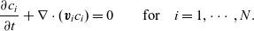 \begin{eqnarray}\frac{\partial c_i}{\partial t} + \nabla \cdot ( \textbf{v}_ic_i)=0 \qquad \mbox{for} \quad i=1,\cdots,N .\end{eqnarray}
A force balance on the entire mixture can be obtained by adding together the N relations (2.23) and noting that
 $\sum_{i=1}^N \hat{\textbf{d}}_i=\textbf{0}$
, to give
$\sum_{i=1}^N \hat{\textbf{d}}_i=\textbf{0}$
, to give
 \begin{eqnarray*}\sum_{i=1}^N c_i \nabla\bar{\mu}_i + \left(\sum_{i=1}^N V_i c_i\right) \nabla p = \textbf{0}.\end{eqnarray*}
By substituting for
 $\sum_{i=1}^N V_i c_i$
from the equation of state (2.20) and for the electrochemical potential from (2.24), we obtain the following expression for the total force balance:
$\sum_{i=1}^N V_i c_i$
from the equation of state (2.20) and for the electrochemical potential from (2.24), we obtain the following expression for the total force balance:
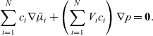
 \begin{eqnarray}\left(\sum_{i=1}^N c_i \nabla {\mu}_i \right) + \left(\sum_{i=1}^N F z_i c_i \right) \nabla \phi +\nabla p = \textbf{0}. \end{eqnarray}
It is straightforward to show from the Gibbs–Duhem relation between the chemical potentials, namely
 \begin{eqnarray*}\sum_{i=1}^N c_i \frac{\partial {\mu}_i}{\partial c_p}=0,\end{eqnarray*}
as derived in Appendix A, that, since
 $\mu_i=\mu_i(c_1,c_2,\cdots c_N)$
,
$\mu_i=\mu_i(c_1,c_2,\cdots c_N)$
,
 \begin{eqnarray}\sum_{i=1}^N c_i \nabla {\mu}_i = \textbf{0}.\end{eqnarray}
This result implies that gradients in the chemical potential, in isolation, do not, as might be expected, lead to a net force on the mixture. In turn this means that the pressure equation (2.26) can be simplified to
 \begin{eqnarray}\nabla p = -\rho \nabla \phi \quad \mbox{where} \quad \rho=\sum_{i=1}^N F z_i c_i . \end{eqnarray}
in which
 $\rho$
represents the charge density of the mixture.
$\rho$
represents the charge density of the mixture.
It is worth making some brief comments about (2.28) which gives an intuitively appealing balance between electrostatic forces and pressure forces acting on the mixture. By taking the curl of (2.28), it is clear that it can only be satisfied if
 $\nabla \rho \times \nabla \phi =\textbf{0}$
(i.e. the gradient of the charge density lies parallel to the electric field
$\nabla \rho \times \nabla \phi =\textbf{0}$
(i.e. the gradient of the charge density lies parallel to the electric field
 $\textbf{E}=-\nabla \phi$
). There are two special cases where this relation is automatically satisfied which are particularly relevant here. The first of these is where
$\textbf{E}=-\nabla \phi$
). There are two special cases where this relation is automatically satisfied which are particularly relevant here. The first of these is where
 $\rho =0$
(or is negligible), and in this instance no pressure gradient is required to balance the electric force on the mixture and so results in a spatially uniform pressure; this is the case that applies to charge-neutral elecrolytes and so is pertinent to battery modelling. The second special case is where the problem is strictly one-dimensional when the pressure gradient simply counteracts the electrical force on the mixture. This is the same situation as occurs in one-dimensional fluid flow where incompressibility dictates that the motion is determined by the concentrations without reference to any forces and is discussed in the context of other such multiphase systems in [Reference Drew27].
$\rho =0$
(or is negligible), and in this instance no pressure gradient is required to balance the electric force on the mixture and so results in a spatially uniform pressure; this is the case that applies to charge-neutral elecrolytes and so is pertinent to battery modelling. The second special case is where the problem is strictly one-dimensional when the pressure gradient simply counteracts the electrical force on the mixture. This is the same situation as occurs in one-dimensional fluid flow where incompressibility dictates that the motion is determined by the concentrations without reference to any forces and is discussed in the context of other such multiphase systems in [Reference Drew27].
In more general cases, the force balances, described above in (2.23), are too naive and need to be supplemented by multiphase viscous dissipation terms as described in [Reference Drew27]. Such issues, however, are beyond the scope of this work, but they are addressed in this context in [Reference Liu and Monroe61].
A final comment about the general moderately concentrated problem is that the electrochemical potential of the i’th species
 $\bar{\mu}_i$
has essentially the same form as that written down for a dilute 1:1 solute in (2.12). The only modification is that the species mole fraction
$\bar{\mu}_i$
has essentially the same form as that written down for a dilute 1:1 solute in (2.12). The only modification is that the species mole fraction
 $c_i/c_T$
is replaced by its activity
$c_i/c_T$
is replaced by its activity
 $a_i$
to reflect the fact that the solution is non-ideal. Hence, we find
$a_i$
to reflect the fact that the solution is non-ideal. Hence, we find
 \begin{eqnarray}\bar{\mu}_i=\mu_i^0 + RT \log(a_i) + z_i F \phi ,\end{eqnarray}
where
 $z_i$
is again the charge state of the i’th species.
$z_i$
is again the charge state of the i’th species.
2.2.2 Stefan–Maxwell equations for a binary 1:1 electrolyte
We now take the general theory of Section 2.2.1 and restrict attention to the case of a 1:1 electrolyte comprised of a solution of Li
 $^+$
ions and a generic negative counter ion species dissolved in a single solvent species. Although battery electrolytes are often based on rather complex solvent mixtures, which are usually closely guarded industrial secrets, this approach provides a reasonable description of many battery electrolytes. In Figure 2, we parameterise the model against experimental data for the most common lithium ion electrolyte LiPF
$^+$
ions and a generic negative counter ion species dissolved in a single solvent species. Although battery electrolytes are often based on rather complex solvent mixtures, which are usually closely guarded industrial secrets, this approach provides a reasonable description of many battery electrolytes. In Figure 2, we parameterise the model against experimental data for the most common lithium ion electrolyte LiPF
 $_6$
in 1:1 EC:DMC from [Reference Valøen and Reimers98], treating the two component solvent (EC:DMC) as if it they were a single solvent.
$_6$
in 1:1 EC:DMC from [Reference Valøen and Reimers98], treating the two component solvent (EC:DMC) as if it they were a single solvent.
In line with [Reference Newman and Thomas-Alyea69], we denote the three species making up the electrolyte, namely the solvent, the
 ${\rm Li}^+$
ions and the generic counterions, by the subscripts
${\rm Li}^+$
ions and the generic counterions, by the subscripts
 $i=0,p,n$
, respectively. We have therefore
$i=0,p,n$
, respectively. We have therefore
 $z_0=0$
,
$z_0=0$
,
 $z_p=1$
and
$z_p=1$
and
 $z_n=-1$
. Combining (2.21)–(2.23) and expanding in component form yields
$z_n=-1$
. Combining (2.21)–(2.23) and expanding in component form yields
 \begin{eqnarray}-c_p \nabla \bar{\mu}_p= \mathcal{K}_{pn}(\textbf{v}_p-\textbf{v}_n)+\mathcal{K}_{p0}(\textbf{v}_p-\textbf{v}_0)+V_p c_p \nabla p,\end{eqnarray}
 \begin{eqnarray}-c_n \nabla \bar{\mu}_n=\mathcal{K}_{np}(\textbf{v}_n-\textbf{v}_p)+\mathcal{K}_{n0}(\textbf{v}_n-\textbf{v}_0)+V_n c_n \nabla p,\end{eqnarray}
 \begin{eqnarray}-c_0 \nabla \bar{\mu}_0=\mathcal{K}_{0p}(\textbf{v}_0-\textbf{v}_p)+\mathcal{K}_{0n}(\textbf{v}_0-\textbf{v}_n)+V_0 c_0 \nabla p,\end{eqnarray}
where, by using (2.21) (i.e.
 $c_T=c_0+c_p+c_n$
) and (2.22)–(2.23), the drag coefficients can be expressed in the form:
$c_T=c_0+c_p+c_n$
) and (2.22)–(2.23), the drag coefficients can be expressed in the form:
 \begin{eqnarray}\mathcal{K}_{ij}=RT\frac{c_i c_j}{c_T D_{ij}} = \mathcal{K}_{ji}, \qquad \mbox{with} \quad i=0,p,n,\quad j=0,p,n.\end{eqnarray}
We note that the three equations (2.30a)–(2.30c) are not independent, as can be seen by adding the three equations together. The result of this operation is an equation that can be shown to be always true by appealing to the Gibbs–Duhem equation, see for example [Reference Atkins, De Paula and Keeler2, Reference Newman and Thomas-Alyea69].
Henceforth, we can omit (2.30c), noting that the choice of physically realistic functions
 $\bar{\mu}_k$
(with
$\bar{\mu}_k$
(with
 $k=0,n,p$
) ensures that this is satisfied. Using (2.29), the electrochemical potentials of the three species are
$k=0,n,p$
) ensures that this is satisfied. Using (2.29), the electrochemical potentials of the three species are
 \begin{eqnarray} \bar{\mu}_{n}&=&\mu_n^0 + RT \log(a_n) - F\phi, \qquad \bar{\mu}_p=\mu_p^0 + RT \log(a_p) + F\phi,\end{eqnarray}
 \begin{eqnarray} \bar{\mu}_0&=&\mu_0^0 +RT \log(a_0). \end{eqnarray}
Note that the pressure terms can be incorporated into the electrochemical potentials yielding modified chemical potentials (denoted by a prime) that read
 \begin{eqnarray}\bar{\mu}'_{\!\!n}&=&\mu_n^0 +V_n p+ RT \log(a_n) - F\phi, \qquad \bar{\mu}'_{\!\!p}=\mu_p^0 +V_p p+ RT \log(a_p) + F\phi, \end{eqnarray}
 \begin{eqnarray} \bar{\mu}'_{\!\!0}&=&\mu_0^0 + V_0 p + RT \log(a_0). \end{eqnarray}
These (modified) electrochemical potentials are actually those that should be used in the Stefan–Maxwell equations given in [Reference Newman and Thomas-Alyea69] (i.e. equations (2.30a)–(2.30c) from which the terms involving
 $\nabla p$
have been removed). Indeed the definition (2.34)–(2.35) are consistent with the true definition of the chemical potential, with a variable pressure (see for example p. 163 of [Reference Atkins, De Paula and Keeler2]), for which the thermodynamic relation
$\nabla p$
have been removed). Indeed the definition (2.34)–(2.35) are consistent with the true definition of the chemical potential, with a variable pressure (see for example p. 163 of [Reference Atkins, De Paula and Keeler2]), for which the thermodynamic relation
 $\partial \mu_i/\partial p = V_i$
is satisfied. However, since most people are more familiar with the definitions (2.32)–(2.33) for solutions, we stick with these.
$\partial \mu_i/\partial p = V_i$
is satisfied. However, since most people are more familiar with the definitions (2.32)–(2.33) for solutions, we stick with these.
Equations (2.30a)–(2.30c) and (2.32)–(2.33) give a consistent description of transport within the entire electrolyte, when coupled to Poisson’s equation which enables the electric potential to be determined from the charge density. However, in practice, throughout nearly all of the electrolyte, there is almost exact charge neutrality (a consequence of Poisson’s equation) which implies that to a very good approximation:
 \begin{eqnarray}c_n= c_p= c .\end{eqnarray}
The only exception to this occurs in the double layers, around the edge of the electrolyte. Since the width of these double layers is typically less than a couple of nanometers, they are usually neglected in the context of electrolyte modelling, their effects only making themselves felt through the phenomenological Butler–Volmer boundary condition. As discussed above, where the electrolyte is charge neutral (i.e.
 $c_n=c_p$
), the solution to the pressure equation (2.28) is such that p is constant meaning that the pressure gradient terms in (2.30a)–(2.30c) vanish.
$c_n=c_p$
), the solution to the pressure equation (2.28) is such that p is constant meaning that the pressure gradient terms in (2.30a)–(2.30c) vanish.
We now seek to find a constitutive equation for the current density
 $\textbf{j}$
. We will broadly follow the derivation given in [Reference Newman and Thomas-Alyea69] but attempt to clarify their argument. As in the dilute case, the current density is given by (2.10), which can be rewritten as:
$\textbf{j}$
. We will broadly follow the derivation given in [Reference Newman and Thomas-Alyea69] but attempt to clarify their argument. As in the dilute case, the current density is given by (2.10), which can be rewritten as:
 \begin{eqnarray}\textbf{j}=Fc(\textbf{v}_p-\textbf{v}_n) .\end{eqnarray}
Substitution of (2.37) into (2.30a) and (2.30b), taking account of (2.36) and the fact that the pressure gradient terms vanish, yields
 \begin{eqnarray}-c\nabla \bar{\mu}_p=\mathcal{K}_{p0}(\textbf{v}_p-\textbf{v}_0)+\frac{\mathcal{K}_{pn}}{Fc} \textbf{j} ,\end{eqnarray}
 \begin{eqnarray}-c\nabla \bar{\mu}_n=\mathcal{K}_{n0}(\textbf{v}_n-\textbf{v}_0)-\frac{\mathcal{K}_{np}}{Fc} \textbf{j} ,\end{eqnarray}
where
 \begin{eqnarray}\mathcal{K}_{pn}=\mathcal{K}_{np}=\frac{RT c^2}{c_T D_{pn}}, \quad \mathcal{K}_{p0}=\frac{RT c c_0}{c_T D_{p0}}, \quad \mathcal{K}_{n0}=\frac{RT c c_0}{c_T D_{n0}} \ \ \mbox{and} \ \ c_T=(c_0+2c).\end{eqnarray}
Equations (2.37), (2.38a) and (2.38b) can be re-arranged to give expressions for the ion velocities in terms of the solvent velocity:
 \begin{eqnarray}\textbf{v}_p=\textbf{v}_0-\frac{c_T}{RT}\frac{D_{p0}}{c_0}\nabla \bar{\mu}_p-\frac{D_{p0}}{D_{pn}F c_0}\textbf{j} ,\end{eqnarray}
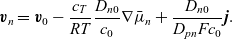 \begin{eqnarray}\textbf{v}_n=\textbf{v}_0-\frac{c_T}{RT}\frac{D_{n0}}{c_0}\nabla \bar{\mu}_n+\frac{D_{n0}}{D_{pn}F c_0}\textbf{j} .\end{eqnarray}
Subtracting (2.40b) from (2.40a) gives
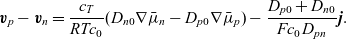 \begin{eqnarray}\textbf{v}_p - \textbf{v}_n=\frac{c_T}{RT c_0}(D_{n0}\nabla\bar{\mu}_n-D_{p0}\nabla\bar{\mu}_p)-\frac{D_{p0}+D_{n0}}{F c_0 D_{pn}}\textbf{j}. \end{eqnarray}
On substituting for
 $\textbf{v}_p-\textbf{v}_n$
(in terms of
$\textbf{v}_p-\textbf{v}_n$
(in terms of
 $\textbf{j}$
) from (2.37), and for
$\textbf{j}$
) from (2.37), and for
 $\bar{\mu}_p$
and
$\bar{\mu}_p$
and
 $\bar{\mu}_n$
from (2.32), and rearranging the resulting expression, we obtain the following expression for
$\bar{\mu}_n$
from (2.32), and rearranging the resulting expression, we obtain the following expression for
 $\textbf{j}$
:
$\textbf{j}$
:
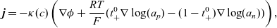 \begin{eqnarray}\textbf{j} = -\kappa(c) \left( \nabla \phi + \frac{RT}{F} ( t_{+}^{0} \nabla \log(a_p) - (1-t_{+}^{0}) \nabla \log(a_n)) \right),\end{eqnarray}
where
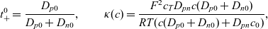 \begin{eqnarray}t_{+}^{0}=\frac{D_{p0}}{D_{p0}+D_{n0}}, \qquad \kappa(c)=\frac{F^2 c_T D_{pn} c (D_{p0}+D_{n0})}{RT(c(D_{p0}+D_{n0})+D_{pn} c_0 )},\end{eqnarray}
are the transference number of the (positive) lithium ions with respect to the solvent velocity, and the conductivity of the electrolyte as a function of the concentration. Note how this equation for
 $\textbf{j}$
, and the definition of transference number and conductivity compare to the dilute version given in (2.11a)–(2.11c).
$\textbf{j}$
, and the definition of transference number and conductivity compare to the dilute version given in (2.11a)–(2.11c).
We now rewrite equations (2.40a)–(2.40b) in a form that avoids the use of a chemical potential for each ion species and instead uses a chemical potential for the entire electrolyte
 $\mu_e$
. Without any loss of generality, we can express
$\mu_e$
. Without any loss of generality, we can express
 $\textbf{v}_p$
and
$\textbf{v}_p$
and
 $\textbf{v}_n$
in the form:
$\textbf{v}_n$
in the form:
 \begin{eqnarray}\begin{array}{l}\displaystyle \textbf{v}_p=((1-\alpha) \textbf{v}_p+\alpha \textbf{v}_n) +\alpha(\textbf{v}_p-\textbf{v}_n), \\ \displaystyle \textbf{v}_n=((1-\alpha) \textbf{v}_p+\alpha \textbf{v}_n)-(1-\alpha)(\textbf{v}_p-\textbf{v}_n),\end{array}\end{eqnarray}
for any function
 $\alpha$
. Our procedure is to substitute
$\alpha$
. Our procedure is to substitute
 $\textbf{v}_p-\textbf{v}_n=\textbf{j}/(Fc)$
in the final terms of these expressions and then to replace
$\textbf{v}_p-\textbf{v}_n=\textbf{j}/(Fc)$
in the final terms of these expressions and then to replace
 $\textbf{v}_n$
and
$\textbf{v}_n$
and
 $\textbf{v}_p$
, everywhere else on the right-hand side of these expressions, from (2.40a) and (2.40b). Choosing
$\textbf{v}_p$
, everywhere else on the right-hand side of these expressions, from (2.40a) and (2.40b). Choosing
 $\alpha=t_{+}^{0}$
, as defined in (2.43), allows the electric potential
$\alpha=t_{+}^{0}$
, as defined in (2.43), allows the electric potential
 $\phi$
to be eliminated from the term
$\phi$
to be eliminated from the term
 $(1-\alpha) \textbf{v}_p+\alpha \textbf{v}_n$
. The expressions for
$(1-\alpha) \textbf{v}_p+\alpha \textbf{v}_n$
. The expressions for
 $\textbf{v}_p$
and
$\textbf{v}_p$
and
 $\textbf{v}_n$
, in (2.44), can then be rewritten in the form:
$\textbf{v}_n$
, in (2.44), can then be rewritten in the form:
 \begin{eqnarray}\textbf{v}_p=\textbf{v}_0-\frac{c_T}{RT c_0}\frac{D_{n0}D_{p0}}{D_{p0}+D_{n0}}(\nabla \bar{\mu}_p+\nabla \bar{\mu}_n)+\frac{t_{+}^{0}}{Fc}\textbf{j} ,\end{eqnarray}
 \begin{eqnarray}\textbf{v}_n=\textbf{v}_0-\frac{c_T}{RT c_0}\frac{D_{n0} D_{p0}}{D_{p0}+D_{n0}}(\nabla \bar{\mu}_p+\nabla \bar{\mu}_n)-\frac{(1-t_{+}^{0})}{Fc}\textbf{j} .\end{eqnarray}
These equations can be further simplified by introducing the electrolyte chemical potential
 $\mu_e(c)$
(a function of electrolyte concentration only) and the chemical diffusion coefficient
$\mu_e(c)$
(a function of electrolyte concentration only) and the chemical diffusion coefficient
 $\mathcal{D}$
, as we did in (2.9), defined by:
$\mathcal{D}$
, as we did in (2.9), defined by:
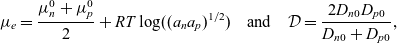 \begin{eqnarray}\mu_e=\frac{\mu^0_n+\mu^0_p}{2}+RT \log((a_n a_p)^{1/2}) \quad \mbox{and} \quad \mathcal{D}=\frac{2D_{n0}D_{p0}}{D_{n0}+D_{p0}}, \end{eqnarray}
and noting that, from (2.32),
 $\mu_e=\frac{1}{2}(\bar{\mu}_p+\bar{\mu}_n)$
. We then find that (2.45a)–(2.45b) can be rewritten in the form:
$\mu_e=\frac{1}{2}(\bar{\mu}_p+\bar{\mu}_n)$
. We then find that (2.45a)–(2.45b) can be rewritten in the form:
 \begin{eqnarray}\textbf{v}_p &=&\textbf{v}_0-\frac{c_T}{c_0 RT} \mathcal{D}\nabla \mu_e+\frac{t_{+}^{0}}{Fc}\textbf{j}, \end{eqnarray}
 \begin{eqnarray}\textbf{v}_n &=&\textbf{v}_0-\frac{c_T}{c_0 RT} \mathcal{D}\nabla \mu_e-\frac{(1-t_{+}^{0})}{Fc}\textbf{j}.\end{eqnarray}
Notably,
 $D_{n0}$
and
$D_{n0}$
and
 $D_{p0}$
can vary with concentration independently, without affecting the preceding analysis. It follows that
$D_{p0}$
can vary with concentration independently, without affecting the preceding analysis. It follows that
 $\mathcal{D}$
and
$\mathcal{D}$
and
 $t_{+}^{0}$
may also vary independently as functions of concentration.
$t_{+}^{0}$
may also vary independently as functions of concentration.
The remaining equations governing the behaviour come from considering conservation of the ions and solvent as well as the volume they occupy. The mass conservation equations for the two ion species are the same as (2.25), namely
 \begin{eqnarray}\frac{\partial c}{\partial t}+\nabla\cdot(c\textbf{v}_p)=0, \quad\frac{\partial c}{\partial t}+\nabla\cdot(c\textbf{v}_n)=0.\end{eqnarray}
Taking the differences of these two equations, and substituting for
 $\textbf{v}_p-\textbf{v}_n$
from (2.37), yields an equation for current conservation:
$\textbf{v}_p-\textbf{v}_n$
from (2.37), yields an equation for current conservation:
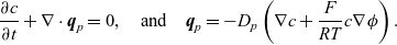
 \begin{eqnarray}\nabla \cdot\textbf{j}=0.\end{eqnarray}
Substituting
 $\textbf{v}_p$
(from (2.47a)) in (2.48) yieldsFootnote
2
$\textbf{v}_p$
(from (2.47a)) in (2.48) yieldsFootnote
2
 \begin{eqnarray}\frac{\partial c}{\partial t} - \nabla\cdot\left( \frac{c_T}{c_0 RT}c\mathcal{D} \nabla \mu_e\right)+\nabla\cdot(c\textbf{v}_0)=-\frac{\nabla t_{+}^{0}\cdot \textbf{j}}{F},\end{eqnarray}
and this can be compared to its dilute theory counterpart given in (2.9). These equations couple to the mass conservation equation for the solvent which, from (2.25), is given by:
 \begin{eqnarray}\frac{\partial c_0}{\partial t}+\nabla\cdot(c_0 \textbf{v}_0)=0. \end{eqnarray}
Finally, we require an equation of state. On using the charge neutrality condition
 $c_n=c_p=c$
in (2.20), we find that this can be written in the form:
$c_n=c_p=c$
in (2.20), we find that this can be written in the form:
 \begin{eqnarray}V_c c+V_0 c_0 = 1,\end{eqnarray}
where
 $V_c=V_n+V_p$
.
$V_c=V_n+V_p$
.
In one dimension, we now have sufficient equations to specify the problem; these are composed of the five equations (2.42), (2.49), (2.50), (2.51) and (2.52) for the five variables c,
 $c_0$
,
$c_0$
,
 $\phi$
,
$\phi$
,
 $\textbf{j}$
and
$\textbf{j}$
and
 $\textbf{v}_0$
. Note that, in more than one dimension, these equations are not sufficient, at least not in general, as can be seen by multiplying (2.48) by
$\textbf{v}_0$
. Note that, in more than one dimension, these equations are not sufficient, at least not in general, as can be seen by multiplying (2.48) by
 $V_c$
and adding to (2.48) multiplied by
$V_c$
and adding to (2.48) multiplied by
 $V_0$
. On using (2.52) to eliminate the time derivative from the resulting equation, this yields the scalar partial differential equation (PDE):
$V_0$
. On using (2.52) to eliminate the time derivative from the resulting equation, this yields the scalar partial differential equation (PDE):
 \begin{eqnarray}\nabla \cdot ( c V_c \textbf{v}_p + c_0 V_0 \textbf{v}_0 )=0,\end{eqnarray}
which in multiple dimensions is insufficient to determine the vector
 $\textbf{v}_0$
. As has been described in [Reference Drew27], this conservation equation needs to be supplemented by a momentum equation, but this is beyond the scope of this work.
$\textbf{v}_0$
. As has been described in [Reference Drew27], this conservation equation needs to be supplemented by a momentum equation, but this is beyond the scope of this work.
Having posed the governing equations, an additional simplifying assumption is commonly made, which appears to be adequate for most solvent-based battery electrolytes. This consists of assuming that the electrolyte is sufficiently dilute so that
 $c_0 \approx c_T$
in which case (2.52) can be approximated by
$c_0 \approx c_T$
in which case (2.52) can be approximated by
 $c_0 \approx 1/V_0$
and the solvent velocity is small (i.e.
$c_0 \approx 1/V_0$
and the solvent velocity is small (i.e.
 $|\textbf{v}_0| \ll |\textbf{v}_p|$
and
$|\textbf{v}_0| \ll |\textbf{v}_p|$
and
 $|\textbf{v}_0| \ll |\textbf{v}_n|$
). This limit is equivalent to the approximation:
$|\textbf{v}_0| \ll |\textbf{v}_n|$
). This limit is equivalent to the approximation:
 \begin{eqnarray}\textbf{v}_0 \equiv \textbf{0} \end{eqnarray}
and only requires solution of the three equations (2.42), (2.49) and (2.50) for the three variables c,
 $\phi$
and
$\phi$
and
 $\textbf{j}$
(instead of five equations for the five variables in the full model). This assumption also avoids the complication, that arises in multiple dimensions, of requiring to be supplemented by a momentum equation. Note however that, even in this small concentration limit, we still include interphase drag between negative and positive ions. This is because interphase drag is very often significant even at quite at low concentrations (often as low as 0.1 molar which is usually a small mole fraction). It arises because positive and negative ions interact via a strong long-range force (the Coulomb force).
$\textbf{j}$
(instead of five equations for the five variables in the full model). This assumption also avoids the complication, that arises in multiple dimensions, of requiring to be supplemented by a momentum equation. Note however that, even in this small concentration limit, we still include interphase drag between negative and positive ions. This is because interphase drag is very often significant even at quite at low concentrations (often as low as 0.1 molar which is usually a small mole fraction). It arises because positive and negative ions interact via a strong long-range force (the Coulomb force).
2.2.3 The potential measured with respect to a lithium electrode
As in the dilute case, it is useful to reformulate the model in terms of
 $\varphi$
, the potential measured with respect to a lithium electrode (i.e.
$\varphi$
, the potential measured with respect to a lithium electrode (i.e.
 $\varphi$
is the potential measured in the lithium reference electrode). Once again we assume that the reaction (2.14) occurring on the surface of the reference electrode is in quasi-equilibrium so that sum of the electrochemical potentials of compounds on each side of (2.14) are identical (i.e.
$\varphi$
is the potential measured in the lithium reference electrode). Once again we assume that the reaction (2.14) occurring on the surface of the reference electrode is in quasi-equilibrium so that sum of the electrochemical potentials of compounds on each side of (2.14) are identical (i.e.
 $\bar{\mu}_{p}+ \bar{\mu}_{\mbox{e}^-_{\rm ref}}=\mu_{{Li}_{\rm ref}}$
). However, owing to the slightly different definition of
$\bar{\mu}_{p}+ \bar{\mu}_{\mbox{e}^-_{\rm ref}}=\mu_{{Li}_{\rm ref}}$
). However, owing to the slightly different definition of
 $\bar{\mu}_p$
in the moderately concentrated case (compare (2.32) with (2.12)), this leads to a modified version of the relation between
$\bar{\mu}_p$
in the moderately concentrated case (compare (2.32) with (2.12)), this leads to a modified version of the relation between
 $\phi$
and
$\phi$
and
 $\varphi$
, namely
$\varphi$
, namely
 \begin{eqnarray}\phi=\varphi+V_*^0-\frac{1}{F} (\mu_p^0+RT \log(a_p)), \end{eqnarray}
where once again the potential shift is defined by
 $V_*^0=\frac{1}{F} (\mu^0_{{Li}_{\rm ref}}-\mu^0_{\mbox{e}^-_{\rm ref}})$
, as in (2.16). This may be compared to the equivalent formula (2.16) for the dilute electrolyte. On substitution of this expression for
$V_*^0=\frac{1}{F} (\mu^0_{{Li}_{\rm ref}}-\mu^0_{\mbox{e}^-_{\rm ref}})$
, as in (2.16). This may be compared to the equivalent formula (2.16) for the dilute electrolyte. On substitution of this expression for
 $\phi$
into (2.42), we can re-express the constitutive equation for the current density equation in the form:
$\phi$
into (2.42), we can re-express the constitutive equation for the current density equation in the form:
 \begin{eqnarray*}\textbf{j} =-\kappa(c)\left(\nabla \varphi - \frac{RT}{F}(1-t_{+}^{0})(\nabla \log(a_p)+\nabla\log(a_n))\right),\end{eqnarray*}
which, on referring to the definition of the electrolyte chemical potential in (2.46), can be re-expressed as:
 \begin{eqnarray}\textbf{j} =-\kappa(c) \left(\nabla \varphi-\frac{2}{F}(1-t_{+}^{0})\nabla \mu_e\right). \end{eqnarray}
This is a clearer way to write Ohm’s law than (2.42) because it allows
 $\textbf{j}$
to expressed solely in terms of the measurable quantities
$\textbf{j}$
to expressed solely in terms of the measurable quantities
 $\varphi$
and
$\varphi$
and
 $\mu_e$
(notably the activities of the individual ion species
$\mu_e$
(notably the activities of the individual ion species
 $a_n$
and
$a_n$
and
 $a_p$
are not directly measurable). This expression differs slightly from that typically presented by Newman and co-authors because they tend to use the dilute limit of (2.56), namely (2.19).
$a_p$
are not directly measurable). This expression differs slightly from that typically presented by Newman and co-authors because they tend to use the dilute limit of (2.56), namely (2.19).
Electrochemical potentials of the ion species.
By substituting (2.55) into (2.32), we obtain expressions for the electrochemical potentials of the two ion species in terms of
 $\varphi$
, the potential measured with respect to a lithium electrode, which are as before:
$\varphi$
, the potential measured with respect to a lithium electrode, which are as before:
 \begin{eqnarray}\bar{\mu}_p=F (\varphi+V_*^0), \qquad \bar{\mu}_n=2 \mu_e(c) - F (\varphi+V_*^0). \end{eqnarray}
2.3 Summary: model for a moderately concentrated electrolyte
The moderately concentrated theory is relevant in those situations where the salt concentration is small compared to the solvent concentration so that
 $c{\ll}c_T$
, the interactions forces are large
$c{\ll}c_T$
, the interactions forces are large
 $(D_{n0} + D_{p0}){\gg}D_{pn}$
, and the solvent velocity can be neglected
$(D_{n0} + D_{p0}){\gg}D_{pn}$
, and the solvent velocity can be neglected
 $\textbf{v}_0 {\approx} 0$
. In this limit, the moderately concentrated charge transport model (2.49), (2.50) and (2.56) takes the form:
$\textbf{v}_0 {\approx} 0$
. In this limit, the moderately concentrated charge transport model (2.49), (2.50) and (2.56) takes the form:
 \begin{eqnarray}\frac{\partial c}{\partial t} - \nabla\cdot\left( {c\mathcal{D}(c) } \nabla \left( \frac{\mu_e(c)}{RT} \right)\right) &=&-\frac{\nabla t_{+}^{0}\cdot \textbf{j}}{F} ,\end{eqnarray}
 \begin{eqnarray}\nabla \cdot \textbf{j} &=& 0 ,\end{eqnarray}
 \begin{eqnarray}\textbf{j} &=&-\kappa(c) \left(\nabla \varphi-\frac{2 RT}{F}(1-t_{+}^{0})\nabla \left( \frac{\mu_e(c)}{RT} \right) \right),\end{eqnarray}
where
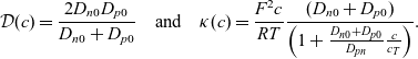 \begin{eqnarray}\mathcal{D}(c)=\frac{{2}D_{n0} D_{p0}}{D_{n0} + D_{p0}} \quad \mbox{and} \quad \kappa(c)=\frac{F^2 c}{RT} \frac{(D_{n0} + D_{p0})}{\left(1+\frac{D_{n0} + D_{p0}}{D_{pn}} \frac{c}{c_T} \right)}.\end{eqnarray}
Note that if we consider the limit of a dilute electrolyte with
 $c{\ll}c_T$
, and the interaction forces are not large
$c{\ll}c_T$
, and the interaction forces are not large
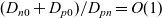 $(D_{n0} + D_{p0})/D_{pn}=O(1)$
, then we revert to the dilute solution model (2.9) and (2.19) provided that we identify
$(D_{n0} + D_{p0})/D_{pn}=O(1)$
, then we revert to the dilute solution model (2.9) and (2.19) provided that we identify
 $D_{p0}$
with
$D_{p0}$
with
 $D_p$
and
$D_p$
and
 $D_{n0}$
with
$D_{n0}$
with
 $D_n$
. We emphasise that even though the widely used name ‘moderately-concentrated’ might lead one to think that the distinction between it and dilute theory is in the assumption on the relative ionic concentrations, it is in fact the assumption made on the size of the interaction forces that sets the two theories apart. An important upshot is the moderately concentrated theory gives good predictions of a larger range of concentrations than dilute theory.
$D_n$
. We emphasise that even though the widely used name ‘moderately-concentrated’ might lead one to think that the distinction between it and dilute theory is in the assumption on the relative ionic concentrations, it is in fact the assumption made on the size of the interaction forces that sets the two theories apart. An important upshot is the moderately concentrated theory gives good predictions of a larger range of concentrations than dilute theory.
It is worth noting that (2.58a)–(2.58c) can be rewritten in the commonly used form:
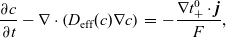 \begin{eqnarray}\frac{\partial c}{\partial t} - \nabla\cdot\left( {D_{\rm eff}}(c) \nabla c \right) &=&-\frac{\nabla t_{+}^{0}\cdot \textbf{j}}{F} ,\end{eqnarray}
 \begin{eqnarray}\nabla \cdot \textbf{j} &=& 0 ,\end{eqnarray}
 \begin{eqnarray}\textbf{j} &=&-\kappa(c) \left(\nabla \varphi-\frac{2 RT}{F}(1-t_{+}^{0}) \frac{a'_{\!\!e}(c)}{a_e(c)}\nabla c \right),\end{eqnarray}
where
 $a_e(c)=(a_n a_p)^{1/2}$
is the activity coefficient of the electrolyte (such that
$a_e(c)=(a_n a_p)^{1/2}$
is the activity coefficient of the electrolyte (such that
 $\mu_e(c)=\mu_e^0+RT \log( a_e(c))$
) and the effective diffusivity is given by:
$\mu_e(c)=\mu_e^0+RT \log( a_e(c))$
) and the effective diffusivity is given by:
 \begin{eqnarray*}{D_{\rm eff}}(c)= \mathcal{D}(c) \frac{c a'_{\!\!e}(c)}{a_e(c)}.\end{eqnarray*}
An implicit assumption in Newman’s formulation of the equations is that the salt solution behaves as an ideal solution so that
 ${a'_{\!\!e}(c)}/{a_e(c)}=1/c$
. Note also that the final terms (on the r.h.s.) of (2.58c) and (2.60c) are commonly written in terms of the mean molal activity coefficient of the salt
${a'_{\!\!e}(c)}/{a_e(c)}=1/c$
. Note also that the final terms (on the r.h.s.) of (2.58c) and (2.60c) are commonly written in terms of the mean molal activity coefficient of the salt
 $f_{\pm}$
, see for example p. 104 of [Reference Plett74], using the identity:
$f_{\pm}$
, see for example p. 104 of [Reference Plett74], using the identity:
 \begin{eqnarray}\nabla \mu_e=RT \frac{a'_{\!\!e}(c)}{a_e(c)}\nabla c=RT \left( 1+ \frac{\partial \log f_\pm}{\partial \log c} \right) \nabla \log c. \end{eqnarray}
To fit the model, it is necessary to determine the lithium diffusivity
 ${D_{\rm eff}}(c)$
, the electrolyte conductivity
${D_{\rm eff}}(c)$
, the electrolyte conductivity
 $\kappa(c)$
and the transference number
$\kappa(c)$
and the transference number
 $t_{+}^{0}(c)$
. Doing this function fitting leads to a relatively robust way of modelling the electrolyte for engineering applications. An example of fitting the phenomenological model functions
$t_{+}^{0}(c)$
. Doing this function fitting leads to a relatively robust way of modelling the electrolyte for engineering applications. An example of fitting the phenomenological model functions
 ${D_{\rm eff}}(c)$
and
${D_{\rm eff}}(c)$
and
 $\kappa(c)$
to data is shown in Figure 2 for the electrolyte LiPF
$\kappa(c)$
to data is shown in Figure 2 for the electrolyte LiPF
 $_{6}$
in 1:1 EC:DMC at
$_{6}$
in 1:1 EC:DMC at
 $T=293$
K (these data come from [Reference Valøen and Reimers98]). For this electrolyte, the transference number of lithium ions, with respect to the solvent velocity, is found to be approximately constant with
$T=293$
K (these data come from [Reference Valøen and Reimers98]). For this electrolyte, the transference number of lithium ions, with respect to the solvent velocity, is found to be approximately constant with
 $t_{+}^{0}=0.38$
.
$t_{+}^{0}=0.38$
.
3. Lithium transport and electric current flow through the electrode particles
Here, we review the modelling of lithium transport in individual electrode particles and current transport through the solid matrix formed by the agglomeration of electrode particles, polymer binder material and conductivity enhancers (such as carbon black). Transport of lithium through the microscopic electrode particles is typically slow; the diffusion timescale for a lithium ion traversing a microscopic electrode particle frequently being comparable to, or even longer, than that required for a lithium ion to traverse the whole cell in the electrolyte. Since the concentration of lithium ions at the surface of the electrode particles strongly influences the rate at which lithium ions are intercalated into the electrode particles from the electrolyte (or vice versa), a battery charge transport model must treat both microscopic transport of lithium through the electrode particles and its macroscopic transport thorough the electrolyte. The coupling between these micro- and macro-scale transport processes occurs via a reaction rate condition which specifies the rate of lithium intercalation (or de-intercalation) at the particle surface in terms of (a) the lithium concentration
 $c_s$
on the surface, (b) the potential difference
$c_s$
on the surface, (b) the potential difference
 $\phi_s-\phi$
between the particle surface and the adjacent electrolyte,Footnote
3
and (c) the lithium concentration c in the adjacent electrolyte. The condition that is typically used in practice is the Butler–Volmer relation (see, for example, [Reference Bockris and Reddy10], which accounts for both the reaction rates and the effects of the double layer, and is based on the quantum mechanical Marcus Theory described in [Reference Marcus65]. Usually, the potential in the electrode matrix
$\phi_s-\phi$
between the particle surface and the adjacent electrolyte,Footnote
3
and (c) the lithium concentration c in the adjacent electrolyte. The condition that is typically used in practice is the Butler–Volmer relation (see, for example, [Reference Bockris and Reddy10], which accounts for both the reaction rates and the effects of the double layer, and is based on the quantum mechanical Marcus Theory described in [Reference Marcus65]. Usually, the potential in the electrode matrix
 $\phi_s$
and the corresponding current density flow
$\phi_s$
and the corresponding current density flow
 $\textbf{j}_s$
through the matrix is modelled by the macroscopic Ohm’s law:
$\textbf{j}_s$
through the matrix is modelled by the macroscopic Ohm’s law:
 \begin{eqnarray}\textbf{j}_s=-\kappa_s \nabla \phi_s, \end{eqnarray}
where
 $\kappa_s$
is the effective conductivity of the electrode matrix (formed of electrode particles, binder and conductivity enhancer).
$\kappa_s$
is the effective conductivity of the electrode matrix (formed of electrode particles, binder and conductivity enhancer).
3.1 The standard approach
Here we set out the standard approach to modelling lithium transport within the electrode particles of a lithium ion cell and the current transfer process between the electrode particles and the surrounding electrolyte. This approach is widely adopted in the modelling literature (e.g. [Reference Dargaville and Farrell19, Reference Doyle, Fuller and Newman25, Reference Doyle, Newman, Gozdz, Schmutz and Tarascon26, Reference Fuller, Doyle and Newman40, Reference Ma, Doyle, Fuller, Doeff, De Jonghe and Newman63, Reference Newman, Thomas, Hafezi and Wheeler70, Reference Srinivasan and Newman92), although it has recently been challenged by an alternative approach which is discussed in Section 3.3.
The central idea of the model is to consider a one-dimensional problem between the two current collectors describing behaviour of the electrolyte and the charge transport in the solid electrodes. The motion of lithium ions within the electrode particles is on a much smaller scale and movement of this is described using a separate dimension representing position within each particle. Here we will use x to represent the position between the current collectors and r to represent the position within any particle. The problem is therefore often referred to as a pseudo-2d model. More precisely, one might describe the structure of the model as being multiscale, where both the micro- and macroscopic models are one-dimensional. Below we present the basic model, deferring its derivation until later.
3.1.1 Microscopic lithium transport models in individual electrode particles
At its very simplest, transport of intercalated lithium within electrode particles is modelled by linear diffusion in an array of uniformly sized (radius a) spheres (see e.g. [Reference Doyle, Newman, Gozdz, Schmutz and Tarascon26]). Hence, the lithium concentration in an electrode particle at position x within the electrode,
 $c_s(r,x,t)$
, evolves according to
$c_s(r,x,t)$
, evolves according to
 \begin{eqnarray}\frac{\partial c_s}{\partial t}= \frac{1}{r^2} \frac{\partial}{\partial r} \left( D_s r^2 \frac{\partial c_s}{\partial r} \right), \qquad \end{eqnarray}
where r measures distance from the particle’s centre and
 $D_s$
is the solid phase Li diffusion coefficient. This model for lithium transport in the electrode particles is typically coupled to the processes taking place in the adjacent electrolyte through a Butler–Volmer relation, which gives the transfer current density
$D_s$
is the solid phase Li diffusion coefficient. This model for lithium transport in the electrode particles is typically coupled to the processes taking place in the adjacent electrolyte through a Butler–Volmer relation, which gives the transfer current density
 $j_{\rm tr}$
flowing out through the surface of the particle, in terms of the lithium concentrations on the particle’s surface
$j_{\rm tr}$
flowing out through the surface of the particle, in terms of the lithium concentrations on the particle’s surface
 $c_s$
, the adjacent electrolyte concentration c and the potential difference between the electrolyte and the electrode particle
$c_s$
, the adjacent electrolyte concentration c and the potential difference between the electrolyte and the electrode particle
 $\varphi-\phi_s$
. Following Faraday’s laws of electrolysis, the flux of lithium on the particle surface is proportional to the current density, leading to the following boundary condition on the electrode particle surface:
$\varphi-\phi_s$
. Following Faraday’s laws of electrolysis, the flux of lithium on the particle surface is proportional to the current density, leading to the following boundary condition on the electrode particle surface:
 \begin{eqnarray*} -D_s \frac{\partial c_s}{\partial r}= \frac{1}{F}\;j_{\rm tr} \qquad\hbox{ on } r=a.\end{eqnarray*}
The use of a linear diffusion model to describe lithium transport within electrode particles is extremely innacurate and it is much better to use a non-linear diffusion equation (with
 $D_s=D_s(c_s)$
) instead, an approach that is adopted in [Reference Farkhondeh and Delacourt31, Reference Karthikeyan, Sikha and White50, Reference Krachkovskiy, Foster, Bazak, Balcom and Goward55], for example. Experimental work demonstrates the strong relationship between diffusivity and lithium ion concentration within certain materials, such as graphite [Reference Baker and Verbrugge4, Reference Levi, Wang, Markevich, Aurbach and Chvoj59, Reference Takami, Satoh, Hara and Ohsaki94, Reference Verbrugge and Koch99] and LiNi
$D_s=D_s(c_s)$
) instead, an approach that is adopted in [Reference Farkhondeh and Delacourt31, Reference Karthikeyan, Sikha and White50, Reference Krachkovskiy, Foster, Bazak, Balcom and Goward55], for example. Experimental work demonstrates the strong relationship between diffusivity and lithium ion concentration within certain materials, such as graphite [Reference Baker and Verbrugge4, Reference Levi, Wang, Markevich, Aurbach and Chvoj59, Reference Takami, Satoh, Hara and Ohsaki94, Reference Verbrugge and Koch99] and LiNi
 $_x$
Mn
$_x$
Mn
 $_y$
Co
$_y$
Co
 $_{1-x-y} O_2$
, often referred to as NMC [Reference Ecker, Käbitz, Laresgoiti and Sauer29, Reference Ecker, Tran, Dechent, Käbitz, Warnecke and Sauer30, Reference Wu, Zhang, Song, Shukla, Liu, Battaglia and Srinivasan101], a positive electrode material discussed in detail in Section 3.3.2. We will also discuss in Sections 3.2 and 3.3 more complicated models of lithium transport applicable to cases where phase separation occurs or the behaviour is highly anisotropic.
$_{1-x-y} O_2$
, often referred to as NMC [Reference Ecker, Käbitz, Laresgoiti and Sauer29, Reference Ecker, Tran, Dechent, Käbitz, Warnecke and Sauer30, Reference Wu, Zhang, Song, Shukla, Liu, Battaglia and Srinivasan101], a positive electrode material discussed in detail in Section 3.3.2. We will also discuss in Sections 3.2 and 3.3 more complicated models of lithium transport applicable to cases where phase separation occurs or the behaviour is highly anisotropic.
3.1.2 The Butler–Volmer equation
The transfer current density
 $j_{\rm tr}$
is the normal component of the current density on the particle surface, directed from the electrode particle into the surrounding electrolyte and is usually expressed in terms of a Butler–Volmer equation (see, e.g [Reference Bockris and Reddy10, Reference Dickinson and Wain23]). This equation quantifies the transfer of lithium ions from the electrode particle material to the electrolyte via the reversible reaction:
$j_{\rm tr}$
is the normal component of the current density on the particle surface, directed from the electrode particle into the surrounding electrolyte and is usually expressed in terms of a Butler–Volmer equation (see, e.g [Reference Bockris and Reddy10, Reference Dickinson and Wain23]). This equation quantifies the transfer of lithium ions from the electrode particle material to the electrolyte via the reversible reaction:
 \begin{eqnarray}\mbox{Li}^+_{(s)} \begin{array}{c} {\scriptstyle v_f}\\ \rightleftharpoons \\{\scriptstyle v_r} \end{array} \mbox{Li}^+_{(l)}, \end{eqnarray}
where
 $\mbox{Li}^+_{(s)}$
denotes a lithium ion in the electrode material and
$\mbox{Li}^+_{(s)}$
denotes a lithium ion in the electrode material and
 $\mbox{Li}^+_{(l)}$
denotes one in the electrolyte. In the vicinity of the electrode–electrolyte interface, lithium ions move in an energy landscape with a form that is represented in Figure 3. In particular, both the forward (from electrode to electrolyte) and reverse (vice-versa) reactions have to overcome a potential barrier. As is typical in these scenarios, the reaction rates can be modelled by an Arrhenius equations (see, e.g. [Reference Bockris and Reddy10] for similar arguments applied to a generic charge transfer reaction). Referring to Figure 3(b), in which the (molar) energy barriers to the transitions from the electrode to the electrolyte (
$\mbox{Li}^+_{(l)}$
denotes one in the electrolyte. In the vicinity of the electrode–electrolyte interface, lithium ions move in an energy landscape with a form that is represented in Figure 3. In particular, both the forward (from electrode to electrolyte) and reverse (vice-versa) reactions have to overcome a potential barrier. As is typical in these scenarios, the reaction rates can be modelled by an Arrhenius equations (see, e.g. [Reference Bockris and Reddy10] for similar arguments applied to a generic charge transfer reaction). Referring to Figure 3(b), in which the (molar) energy barriers to the transitions from the electrode to the electrolyte (
 $\Delta E_f$
) and from the electrolyte to the electrode (
$\Delta E_f$
) and from the electrolyte to the electrode (
 $\Delta E_r$
) are both illustrated, we expect the forward and reverse lithium ion transfer velocities to have the forms:
$\Delta E_r$
) are both illustrated, we expect the forward and reverse lithium ion transfer velocities to have the forms:
 \begin{eqnarray}v_f=v_{f,0} \exp\left(-\frac{\Delta E_f}{RT} \right), \qquad v_r=v_{r,0} \exp\left(-\frac{\Delta E_r}{RT} \right),\end{eqnarray}
Schematic showing the energy landscape that a Li
 $^+$
ion transitions through as it moves from electrode to electrolyte (or vice-versa). (a) In the absence of an electrical potential difference between electrode and electrolyte. (b) With an electrical potential difference
$^+$
ion transitions through as it moves from electrode to electrolyte (or vice-versa). (a) In the absence of an electrical potential difference between electrode and electrolyte. (b) With an electrical potential difference
 $\Delta\phi=\phi_s-\phi$
between electrode and electrolyte.
$\Delta\phi=\phi_s-\phi$
between electrode and electrolyte.
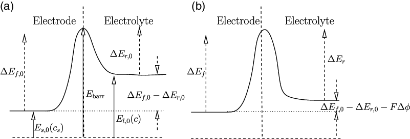
respectively. Since the lithium ion is positively charged, the size of these energy barriers is affected by the (Galvani) potential drop
 $\Delta \phi= \phi_s-\phi$
between the interior of the electrode and the interior of the electrolyte. Indeed it is clear that
$\Delta \phi= \phi_s-\phi$
between the interior of the electrode and the interior of the electrolyte. Indeed it is clear that
 \begin{eqnarray}\Delta E_f-\Delta E_r=\Delta E_{f,0}-\Delta E_{r,0}-F \Delta \phi, \end{eqnarray}
where
 $\Delta E_{f,0}$
and
$\Delta E_{f,0}$
and
 $\Delta E_{r,0}$
are the energy barriers to the forward and reverse reactions when there is no potential difference between the electrode and the electrolyte (i.e.
$\Delta E_{r,0}$
are the energy barriers to the forward and reverse reactions when there is no potential difference between the electrode and the electrolyte (i.e.
 $\Delta \phi=0$
). Notably, since
$\Delta \phi=0$
). Notably, since
 $E_{s,0}$
and
$E_{s,0}$
and
 $E_{l,0}$
are the molar energies of lithium ions in electrode and electrolyte, respectively, we require that
$E_{l,0}$
are the molar energies of lithium ions in electrode and electrolyte, respectively, we require that
 $E_{s,0}=E_{s,0}(c_s)$
and
$E_{s,0}=E_{s,0}(c_s)$
and
 $E_{l,0}=E_{l,0}(c)$
(i.e. they depend only on the lithium concentrations in their respective materials). Furthermore, since
$E_{l,0}=E_{l,0}(c)$
(i.e. they depend only on the lithium concentrations in their respective materials). Furthermore, since
 $\Delta E_{f,0}=E_{\rm barr}-E_{s,0}(c_s)$
and
$\Delta E_{f,0}=E_{\rm barr}-E_{s,0}(c_s)$
and
 $\Delta E_{r,0}=E_{\rm barr}-E_{l,0}(c)$
and since we expect
$\Delta E_{r,0}=E_{\rm barr}-E_{l,0}(c)$
and since we expect
 $E_{\rm barr}$
(the molar energy of the lithium ions at the energy barrier) to be independent of the local lithium concentration (which is always very small there), it follows that
$E_{\rm barr}$
(the molar energy of the lithium ions at the energy barrier) to be independent of the local lithium concentration (which is always very small there), it follows that
 $\Delta E_{f,0}=\Delta E_{f,0}(c_s)$
and
$\Delta E_{f,0}=\Delta E_{f,0}(c_s)$
and
 $\Delta E_{r,0}= \Delta E_{r,0}(c)$
. Turning to the potential difference across the interface it is apparent, from (3.5), that the the potential difference across the interface
$\Delta E_{r,0}= \Delta E_{r,0}(c)$
. Turning to the potential difference across the interface it is apparent, from (3.5), that the the potential difference across the interface
 $\Delta \phi$
is split between the two activation energies, this suggests partitioning it as follows:
$\Delta \phi$
is split between the two activation energies, this suggests partitioning it as follows:
 \begin{eqnarray*}\Delta E_f=\Delta E_{f,0}(c_s)-(1-\beta) F \Delta \phi \quad \mbox{and} \quad \Delta E_r=\Delta E_{r,0}(c)+\beta F \Delta \phi,\end{eqnarray*}
where
 $\beta$
is some constant between 0 and 1 (usually
$\beta$
is some constant between 0 and 1 (usually
 $\beta=1/2$
). We thus expect the transfer current
$\beta=1/2$
). We thus expect the transfer current
 $j_{\rm tr}$
to have the form:
$j_{\rm tr}$
to have the form:
 \begin{eqnarray}j_{\rm tr}=F \left(c_s v_f^*(c_s) \exp \left( \frac{F}{RT} (1-\beta) \Delta \phi \right) -c \left( 1- \frac{c_s}{c_{s,max}} \right) v_r^*(c) \exp \left(- \frac{F}{RT} \beta \Delta \phi \right) \right), \end{eqnarray}
 \begin{eqnarray}\mbox{where} \quad v_f^*(c_s)=v_{f,0} \exp\left(-\frac{\Delta E_{f,0}(c_s)}{RT} \right) \quad \mbox{and} \quad v_r^*(c)=v_{f,0} \exp\left(-\frac{\Delta E_{r,0}(c)}{RT} \right).\end{eqnarray}
Here the factor of
 $\left( 1- {c_s}/{c_{s,\max}} \right)$
in the final term in (3.6) is to account for the fact that the reverse transfer (from the electrolyte to the electrode) is dependent on the availability of sites in the electrode material and so cannot occur if
$\left( 1- {c_s}/{c_{s,\max}} \right)$
in the final term in (3.6) is to account for the fact that the reverse transfer (from the electrolyte to the electrode) is dependent on the availability of sites in the electrode material and so cannot occur if
 $c_s=c_{s,\max}$
and all the sites in the electrode material are already occupied. We can rewrite (3.6) in the more usual form:
$c_s=c_{s,\max}$
and all the sites in the electrode material are already occupied. We can rewrite (3.6) in the more usual form:
 \begin{eqnarray}j_{\rm tr}= i_0(c,c_s) \left( \exp \left( \frac{F}{RT} (1-\beta) \eta \right) - \exp \left(- \frac{F}{RT} \beta \eta \right) \right), \end{eqnarray}
 \begin{eqnarray}\mbox{where} \quad i_0(c,c_s) =F \left( c_s v_f^*(c_s) \right)^{\beta}\left( c v_r^*(c) \left( 1- \frac{c_s}{c_{s,\max}} \right) \right)^{1-\beta}, \end{eqnarray}
where the overpotential
 $\eta$
and the open-circuit potential are defined by:
$\eta$
and the open-circuit potential are defined by:
 \begin{eqnarray}\eta=\phi_s-\phi -u_{eq}(c,c_s), \end{eqnarray}
 \begin{eqnarray}u_{eq}(c,c_s)=\frac{RT}{F} \log (c v_r^*(c))-\frac{RT}{F} \log\left(\frac{c_s v_f^*(c_s)}{\left( 1- \frac{c_s}{c_{s,\max}} \right)} \right), \end{eqnarray}
and we have used the fact that
 $\Delta \phi=\phi_s-\phi$
. We write it in this form to emphasise the fact that
$\Delta \phi=\phi_s-\phi$
. We write it in this form to emphasise the fact that
 $u_{eq}(c,c_s)$
can be written in the form
$u_{eq}(c,c_s)$
can be written in the form
 $u_{eq}(c,c_s)=\mathcal{G}(c)- \mathcal{H}(c_s)$
, where
$u_{eq}(c,c_s)=\mathcal{G}(c)- \mathcal{H}(c_s)$
, where
 $\mathcal{G}$
is a function of c and
$\mathcal{G}$
is a function of c and
 $\mathcal{H}$
is a function of
$\mathcal{H}$
is a function of
 $c_s$
. In the special case where the Galvani potential difference between electrode and electrolyte
$c_s$
. In the special case where the Galvani potential difference between electrode and electrolyte
 $\Delta \phi=\phi_s-\phi$
is held at zero, an equilibrium between the electrode and the electrolyte (at which
$\Delta \phi=\phi_s-\phi$
is held at zero, an equilibrium between the electrode and the electrolyte (at which
 $j_{tr}=0$
) is established when
$j_{tr}=0$
) is established when
 $u_{eq}(c,c_s)=0$
. At this equilibrium, the chemical potential of the lithium ions in the electrolyte
$u_{eq}(c,c_s)=0$
. At this equilibrium, the chemical potential of the lithium ions in the electrolyte
 $\mu_{p}(c)$
is equal to that in the electrode material
$\mu_{p}(c)$
is equal to that in the electrode material
 $\mu_{(s)}(c_s)$
. Given that
$\mu_{(s)}(c_s)$
. Given that
 $u_{eq}(c,c_s)$
has the form
$u_{eq}(c,c_s)$
has the form
 $\mathcal{G}(c)- \mathcal{H}(c_s)$
, and accounting for the dimensions of chemical potentials and
$\mathcal{G}(c)- \mathcal{H}(c_s)$
, and accounting for the dimensions of chemical potentials and
 $u_{eq}$
, this strongly suggests that
$u_{eq}$
, this strongly suggests that
 \begin{eqnarray}F u_{eq}(c,c_s)=\mu_{p}(c)-\mu_{(s)}(c_s).\end{eqnarray}
It then follows that the overpotential can be written in the form:
 \begin{eqnarray}\eta=\phi_s-\phi-\frac{1}{F} \left(\mu_{p}(c)-\mu_{(s)}(c_s) \right), \end{eqnarray}
or equivalently
 \begin{eqnarray}\eta=\frac{1}{F} \left(\bar{\mu}_{(s)}(c_s)-\bar{\mu}_{p}(c) \right),\end{eqnarray}
where
 $\bar{\mu}_{(s)}$
and
$\bar{\mu}_{(s)}$
and
 $\bar{\mu}_{p}$
are the electrochemical potentials of lithium ions in the electrode material and the electrolyte, respectively. This is an intuitively appealing form for the overpotential because it shows that the Butler–Volmer equation (3.8) drives the system towards an equilibrium in which
$\bar{\mu}_{p}$
are the electrochemical potentials of lithium ions in the electrode material and the electrolyte, respectively. This is an intuitively appealing form for the overpotential because it shows that the Butler–Volmer equation (3.8) drives the system towards an equilibrium in which
 $\eta$
vanishes, and in which the electrochemical potentials of lithium ions on either side of the interface are equal and the transfer current
$\eta$
vanishes, and in which the electrochemical potentials of lithium ions on either side of the interface are equal and the transfer current
 $j_{\rm tr}$
switches off. This result is in agreement with the derivation presented in [Reference Latz and Zausch56] and also with the discussion in [Reference Schmickler and Santos83] who note that the “driving force” for the reaction is this difference in the electrochemical potentials. Furthermore, in this form we can substitute for
$j_{\rm tr}$
switches off. This result is in agreement with the derivation presented in [Reference Latz and Zausch56] and also with the discussion in [Reference Schmickler and Santos83] who note that the “driving force” for the reaction is this difference in the electrochemical potentials. Furthermore, in this form we can substitute for
 $\bar{\mu}_{p}$
in terms of
$\bar{\mu}_{p}$
in terms of
 $\varphi$
, from (2.57), and obtain the expression for the overpotential that is typically used in the Butler–Volmer equation, namely
$\varphi$
, from (2.57), and obtain the expression for the overpotential that is typically used in the Butler–Volmer equation, namely
 \begin{eqnarray}\eta=\phi_{\rm s}-\varphi-U_{\rm eq}(c_s)\quad \mbox{where} \quad U_{\rm eq}(c_s)= V_*^0-\frac{1}{F} \mu_{(s)}(c_s). \end{eqnarray}
Notably, on using this definition of
 $U_{eq}(c_s)$
and the relation (3.12), we find the following relationship between
$U_{eq}(c_s)$
and the relation (3.12), we find the following relationship between
 $u_{eq}(c,c_s)$
and
$u_{eq}(c,c_s)$
and
 $U_{eq}(c_s)$
:
$U_{eq}(c_s)$
:
 \begin{eqnarray}U_{\rm eq}(c_{\rm s})=u_{\rm eq}(c,c_{\rm s})+V_*^0-\frac{\mu_p(c)}{F}, \end{eqnarray}
which shows that
 $U_{eq}(c_s)$
inherits the same singularities in
$U_{eq}(c_s)$
inherits the same singularities in
 $c_s$
that
$c_s$
that
 $u_{eq}(c,c_s)$
has. We point out that
$u_{eq}(c,c_s)$
has. We point out that
 $u_{\rm eq}$
is the open-circuit potential and
$u_{\rm eq}$
is the open-circuit potential and
 $U_{\rm eq}$
is the open circuit potential measured with respect to a lithium electrode.
$U_{\rm eq}$
is the open circuit potential measured with respect to a lithium electrode.
The standard form of the Butler–Volmer equations.
The standard way of expressing the Butler–Volmer equation is in terms of the open-circuit potential
 $U_{eq}(c_s)$
, as defined in (3.15), and on referring back to (3.8)–(3.9) we see that it should be written in the form:
$U_{eq}(c_s)$
, as defined in (3.15), and on referring back to (3.8)–(3.9) we see that it should be written in the form:
 \begin{eqnarray}j_{\rm tr}= i_0(c,c_s) \left( \exp \left( \frac{F}{RT} (1-\beta) \eta \right) - \exp \left(- \frac{F}{RT} \beta \eta \right) \right) \qquad \quad \mbox{where}, \end{eqnarray}
 \begin{eqnarray}\eta=\phi_s - \varphi -U_{eq}(c_s), \quad i_0(c,c_s) =F \left( c_s v_f^*(c_s) \right)^{\beta}\left( c v_r^*(c) \left( 1- \frac{c_s}{c_{s,\max}} \right) \right)^{1-\beta}. \end{eqnarray}
It is important to realise that, it is only by expressing the overpotential in terms of a difference between the true electric potential in the electrode
 $\phi_s$
and the potential measured with respect to a lithium electrode in the electrolyte
$\phi_s$
and the potential measured with respect to a lithium electrode in the electrolyte
 $\varphi$
that we obtain an expression for the open-circuit potential
$\varphi$
that we obtain an expression for the open-circuit potential
 $U_{\rm eq}$
that is a function solely of
$U_{\rm eq}$
that is a function solely of
 $c_s$
. Furthermore, it is relatively straightforward to obtain
$c_s$
. Furthermore, it is relatively straightforward to obtain
 $U_{eq}(c_s)$
experimentally, simply by measuring the potential difference
$U_{eq}(c_s)$
experimentally, simply by measuring the potential difference
 $\phi_s-\varphi$
, at steady state (with
$\phi_s-\varphi$
, at steady state (with
 $j_{\rm tr}=0$
) between the electrode material and a lithium reference electrode placed in the electrolyte. The standard expression for the exchange current density
$j_{\rm tr}=0$
) between the electrode material and a lithium reference electrode placed in the electrolyte. The standard expression for the exchange current density
 $i_0(c,c_s)$
is obtained by setting both
$i_0(c,c_s)$
is obtained by setting both
 $v_f^*$
and
$v_f^*$
and
 $v_r^*$
to be constant. Although this is not strictly correct, it does at least ensure that
$v_r^*$
to be constant. Although this is not strictly correct, it does at least ensure that
 $i_0(c,c_s)$
has the correct singularities as
$i_0(c,c_s)$
has the correct singularities as
 $c \rightarrow 0$
,
$c \rightarrow 0$
,
 $c_s \rightarrow 0$
and
$c_s \rightarrow 0$
and
 $c_s \rightarrow c_{s,\max}$
. This is enough, as shown below to ensure reasonable agreement with the real behaviour because the exponential terms in (3.17) usually dominate the behaviour compared to the prefactor
$c_s \rightarrow c_{s,\max}$
. This is enough, as shown below to ensure reasonable agreement with the real behaviour because the exponential terms in (3.17) usually dominate the behaviour compared to the prefactor
 $i_0(c,c_s)$
, except where the latter tends to zero.
$i_0(c,c_s)$
, except where the latter tends to zero.
From a mathematical perspective, it is important to realise that the open-circuit potential measured with respect to a lithium electrode (OCP) should tend to minus infinity as
 $c_s \nearrow c_{\rm s,max}$
and tend to plus infinity as
$c_s \nearrow c_{\rm s,max}$
and tend to plus infinity as
 $c_s\searrow 0$
. This can be seen clearly from the relation between
$c_s\searrow 0$
. This can be seen clearly from the relation between
 $U_{eq}(c_s)$
and
$U_{eq}(c_s)$
and
 $u_{eq}(c,c_s)$
contained in (3.16) and the definition of
$u_{eq}(c,c_s)$
contained in (3.16) and the definition of
 $u_{eq}(c,c_s)$
found in (3.11). It is this property of
$u_{eq}(c,c_s)$
found in (3.11). It is this property of
 $U_{eq}(c_s)$
that stops
$U_{eq}(c_s)$
that stops
 $c_s$
reaching
$c_s$
reaching
 $c_{\rm s,max}$
or 0, rather than the factors of
$c_{\rm s,max}$
or 0, rather than the factors of
 $(1-c_s/c_{\rm s,max})$
and
$(1-c_s/c_{\rm s,max})$
and
 $c_s$
that appears in the exchange current density
$c_s$
that appears in the exchange current density
 $i_0$
(see (3.18b)). Thus, if the experimentally obtained plots of
$i_0$
(see (3.18b)). Thus, if the experimentally obtained plots of
 $U_{eq}(c_s)$
do not display these singularities (which is usually because the experiments do not explore the extreme ends of the range), they should be added in by hand. It is standard to plot the OCP as a function of
$U_{eq}(c_s)$
do not display these singularities (which is usually because the experiments do not explore the extreme ends of the range), they should be added in by hand. It is standard to plot the OCP as a function of
 ${y}=c_s/c_{\rm s,max}$
, where y is termed the lithium stoichiometry. The OCP varies widely depending on the electrode material and to illustrate this it is plotted in Figure 4(a) for the lithiated graphite Li
${y}=c_s/c_{\rm s,max}$
, where y is termed the lithium stoichiometry. The OCP varies widely depending on the electrode material and to illustrate this it is plotted in Figure 4(a) for the lithiated graphite Li
 $_x C_6$
while in Figure 4(b) and (c) it is plotted for lithiated (NLC) Li
$_x C_6$
while in Figure 4(b) and (c) it is plotted for lithiated (NLC) Li
 $_y$
(Ni
$_y$
(Ni
 $_{0.4}$
Co
$_{0.4}$
Co
 $_{0.6}$
)O
$_{0.6}$
)O
 $_2$
, and iron phosphate Li
$_2$
, and iron phosphate Li
 $_y$
FePO
$_y$
FePO
 $_4$
, respectively. Note the OCP for Li
$_4$
, respectively. Note the OCP for Li
 $_y$
FePO
$_y$
FePO
 $_4$
has a large almost flat plateau symptomatic of a two-phase state within the material. Note further that in all the experimental data, at least one of the singularities in
$_4$
has a large almost flat plateau symptomatic of a two-phase state within the material. Note further that in all the experimental data, at least one of the singularities in
 $U_{eq}(c_s)$
is missing.
$U_{eq}(c_s)$
is missing.
The OCP,
 $U_{\rm eq}$
, of (a) LiC
$U_{\rm eq}$
, of (a) LiC
 $_6$
, from [Reference Ecker, Tran, Dechent, Käbitz, Warnecke and Sauer30], (b) LiFePO
$_6$
, from [Reference Ecker, Tran, Dechent, Käbitz, Warnecke and Sauer30], (b) LiFePO
 $_4$
, from [Reference Srinivasan and Newman92]) and (c) Li(Ni
$_4$
, from [Reference Srinivasan and Newman92]) and (c) Li(Ni
 $_{0.4}$
Co
$_{0.4}$
Co
 $_{0.6}$
)O
$_{0.6}$
)O
 $_2$
, from [Reference Ecker, Tran, Dechent, Käbitz, Warnecke and Sauer30]. Each is shown as a function of Lithium stoichiometry.
$_2$
, from [Reference Ecker, Tran, Dechent, Käbitz, Warnecke and Sauer30]. Each is shown as a function of Lithium stoichiometry.
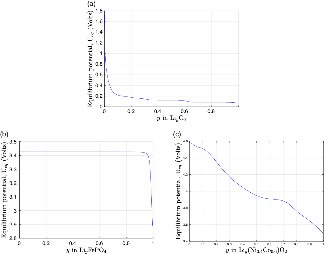
A comment on the functional form for the transfer current.
For the sake of completeness, we write down the form of the transfer current
 $i_0(c,c_s)$
that is logically consistent with the derivation of the Butler–Volmer equation presented above. By comparison of (3.11) with (3.12), we see that
$i_0(c,c_s)$
that is logically consistent with the derivation of the Butler–Volmer equation presented above. By comparison of (3.11) with (3.12), we see that
 $c v_r^*(c)={const.} \exp(\mu_p(c)/RT)$
and
$c v_r^*(c)={const.} \exp(\mu_p(c)/RT)$
and
 $c_s v_f^*(c_s)={const.} (1-c_s/c_{s,\max}) \exp(\mu_{(s)}(c_s)/RT)$
. In addition, on recalling that
$c_s v_f^*(c_s)={const.} (1-c_s/c_{s,\max}) \exp(\mu_{(s)}(c_s)/RT)$
. In addition, on recalling that
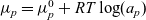 $\mu_p=\mu^0_p+RT \log (a_p)$
, where
$\mu_p=\mu^0_p+RT \log (a_p)$
, where
 $a_p$
is the activity of the lithium ions, and that
$a_p$
is the activity of the lithium ions, and that
 $\mu_{(s)}(c_s)$
is related to
$\mu_{(s)}(c_s)$
is related to
 $U_{eq}(c_s)$
via (3.15), we see that these can be rewritten as:
$U_{eq}(c_s)$
via (3.15), we see that these can be rewritten as:
 \begin{eqnarray*}c v_r^*(c)=const.a_p, \quad \mbox{and} \quad c_s v_f^*(c_s)=const. \left(1-\frac{c_s}{c_{s,\max}} \right) \exp\left(-\frac{F}{RT} U_{eq}(c_s) \right).\end{eqnarray*}
It follows that we can rewrite the transfer current density in (3.18) as:
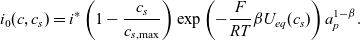 \begin{eqnarray}i_0(c,c_s) =i^* \left( 1- \frac{c_s}{c_{s,\max}} \right) \exp\left(-\frac{F}{RT} \beta U_{eq}(c_s) \right)a_p^{1-\beta}.\end{eqnarray}
for a suitable constant
 $i^*$
with units of current density.
$i^*$
with units of current density.
Behaviour of
 $\,\textbf{j}_{\textbf{tr}}$
close to the extreme cases.
$\,\textbf{j}_{\textbf{tr}}$
close to the extreme cases.
Setting
 $v^*_{\rm r}$
to be constant (as mentioned above) but keeping
$v^*_{\rm r}$
to be constant (as mentioned above) but keeping
 $v^*_{\rm f}$
dependent on
$v^*_{\rm f}$
dependent on
 $c_{\rm s}$
(which seem to be necessary in order to be able to fit open-circuit potential data, measured with respect to a lithium reference electrode), from (3.10), (3.11), (3.16), (3.17) and (3.18) we have that
$c_{\rm s}$
(which seem to be necessary in order to be able to fit open-circuit potential data, measured with respect to a lithium reference electrode), from (3.10), (3.11), (3.16), (3.17) and (3.18) we have that
 \begin{equation*}i_0(c,c_s) =K_0 \left( c_sv^*_{\rm f}(c_{\rm s})\right)^{\beta}\left( c \left( c_{s,\max}- c_s \right) \right)^{1-\beta},\end{equation*}
 \begin{eqnarray*}j_{\rm tr} & = & i_0 \left( \exp \left( \frac{F(1-\beta)}{RT} \left( \phi_{\rm s}-\phi - u_{\rm eq}( c,c_{\rm s})\right) \right) - \exp \left(- \frac{F\beta}{RT} \left( \phi_{\rm s}-\phi - u_{\rm eq}( c,c_{\rm s})\right) \right) \right) \\[4pt] & = & i_0 \left( \exp \left( \frac{F(1-\beta)}{RT} \left( \phi_{\rm s}-\varphi - U_{\rm eq}( c_{\rm s})\right) \right) - \exp \left(- \frac{F\beta}{RT} \left( \phi_{\rm s}-\varphi - U_{\rm eq}( c_{\rm s})\right) \right) \right) ,\end{eqnarray*}
 \begin{equation*}u_{eq}(c,c_s)=\frac{RT}{F} \log \left( \frac{K_1c (c_{\rm s,max} -c_{\rm s})}{c_{\rm s}}\right) + {\mathcal U}_{\rm eq}(c_{\rm s}),\end{equation*}
with
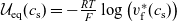 ${\mathcal U}_{\rm eq} (c_{\rm s})= - \frac{RT}{F} \log \left( v^*_{\rm f}(c_{\rm s})\right)$
and, for ideal electrolytes (so that
${\mathcal U}_{\rm eq} (c_{\rm s})= - \frac{RT}{F} \log \left( v^*_{\rm f}(c_{\rm s})\right)$
and, for ideal electrolytes (so that
 $a_p=\frac{c}{c_T}$
),
$a_p=\frac{c}{c_T}$
),
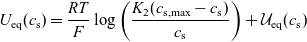 \begin{equation} U_{\rm eq} (c_{\rm s})= \frac{RT}{F} \log \left( \frac{K_2 (c_{\rm s,max} -c_{\rm s})}{c_{\rm s}}\right) + {\mathcal U}_{\rm eq}(c_{\rm s})\end{equation}
for suitable constants
 \begin{equation*}K_0=\frac{F (v^*_{\rm r})^{1-\beta}}{(c_{\rm s,max})^{1-\beta}}, \ K_1=\frac{v^*_{\rm r}}{c_{\rm s,max}} \mbox{ and }K_2=\frac{v^*_{\rm r}c_{\rm T}\exp \left( \frac{F}{RT}V^0_*-\frac{\mu_p^0}{RT}\right)}{c_{\rm s,max}}.\end{equation*}
Therefore, when using the electric potential of the electrolyte (
 $\phi$
), we have
$\phi$
), we have
 \begin{equation} \begin{array}{l}{\displaystyle j_{\rm tr} = \frac{K_0}{K_1^{1-\beta}} c_sv^*_{\rm f}(c_{\rm s})\exp \left( \frac{F(1-\beta)}{RT} \left( \phi_{\rm s}-\phi \right) \right)} \\ {\displaystyle - K_0K_1^\beta c(c_{\rm s,max}-c_{\rm s})\exp \left( -\frac{F\beta}{RT} \left( \phi_{\rm s}-\phi \right) \right)}\end{array}\end{equation}
and, when using the electric potential of the electrolyte measured with respect to a lithium electrode (
 $\varphi$
), we have
$\varphi$
), we have
 \begin{equation} \begin{array}{l}{\displaystyle j_{\rm tr} = \frac{K_0}{K_2^{1-\beta}} c_sv^*_{\rm f}(c_{\rm s})c^{1-\beta}\exp \left( \frac{F(1-\beta)}{RT} \left( \phi_{\rm s}-\varphi \right) \right)} \\ {\displaystyle - K_0K_2^\beta c^{1-\beta}(c_{\rm s,max}-c_{\rm s})\exp \left( -\frac{F\beta}{RT} \left( \phi_{\rm s}-\varphi \right) \right) .} \end{array}\end{equation}
We notice here four important features of this formulation:
-
(1). The open-circuit potential (
 $u_{\rm eq}$
) depends on c and
$c_{\rm s}$
, while the open-circuit potential measured with respect to a lithium electrode (
$U_{\rm eq}$
) only depends on
$c_{\rm s}$
.
$u_{\rm eq}$
) depends on c and
$c_{\rm s}$
, while the open-circuit potential measured with respect to a lithium electrode (
$U_{\rm eq}$
) only depends on
$c_{\rm s}$
. -
(2). If
$c_{\rm s}\rightarrow 0$
, with
$c\neq 0$
(constant) and
$v^*_{\rm f}(c_{\rm s})$
is bounded and greater than a positive constant, then
$i_0\rightarrow 0$
,
$u_{\rm eq}\rightarrow \infty$
and
$U_{\rm eq}\rightarrow \infty$
. Furthermore, as
$c_{\rm s} \to 0$
, from (3.21) or (3.22), we can see that the forward (anodic) reaction is first order, while the reverse (cathodic) reaction is bounded and positive (like a zeroth-order reaction). -
(3). If
$c_{\rm s}\rightarrow c_{\rm s,max}$
, with
$c\neq 0$
(constant) and
$v^*_{\rm f}(c_{\rm s})$
is bounded and greater than a positive constant, then
$i_0\rightarrow 0$
,
$u_{\rm eq}\rightarrow -\infty$
and
$U_{\rm eq}\rightarrow -\infty$
Furthermore, as
$c_{\rm s} \to c_{\rm s,max}$
, from (3.21) or (3.22), we can see that the forward (anodic) reaction is bounded and positive (like a zeroth-order reaction), while the reverse (cathodic) reaction is first order. -
(4). If
$c\rightarrow 0$
, with
$c_{\rm s}\neq 0$
, then
$i_0\rightarrow 0$
and
$u_{\rm eq}\rightarrow -\infty$
but
$U_{\rm eq}$
remains constant. Furthermore, as
$c \to 0$
, from (3.21) we can see that the forward (anodic) reaction is bounded and positive (like a zeroth-order reaction), while the reverse (cathodic) reaction is first order. Nevertheless, this property is not directly seen from (3.22) (i.e. when writing
$j_{\rm tr}$
in terms of the electric potential of the electrolyte measured with respect to a lithium electrode), since that equation is based on the dependence of
$\varphi$
on c, so that
$\varphi \to -\infty$
as
$c\to 0$
in a way consistent with the correct asymptotic behaviour.


These conditions ensure that the lithium flux is constrained to prevent concentrations in the solid being taken into non-physical regimes and also to ensure that, if the solid is nearly fully depleted (or filled) with lithium, that the transfer current is not artificially forced to zero. Thus, a Butler–Volmer relation of this form allows the flux to move the system away from these depleted (and filled) states. This gives a model which is capable of describing battery charge from a completely depleted state or discharge from a fully charged state.
When fitting the various functions characterising the Butler–Volmer equation (3.17) to the data, it is necessary to include the singular behaviours as
 $c\rightarrow 0$
,
$c\rightarrow 0$
,
 $c_{\rm s}\rightarrow 0$
and
$c_{\rm s}\rightarrow 0$
and
 $c_{\rm s}\rightarrow c_{\rm s,max}$
as given previously. Following the approach explained above (see (3.20)), one can take
$c_{\rm s}\rightarrow c_{\rm s,max}$
as given previously. Following the approach explained above (see (3.20)), one can take
 \begin{equation*} U_{\rm eq}(c_{\rm s}) = \frac{RT}{F}\log \left( \frac{c_{\rm s,max}-c_{\rm s}}{c_{\rm s}} \right) + f(c_{\rm s}; a_1, a_2,\cdots , a_N),\end{equation*}
where
 $f(\cdot ; a_1, a_2,\cdots , a_N)$
is some family of suitable functions, and
$f(\cdot ; a_1, a_2,\cdots , a_N)$
is some family of suitable functions, and
 $\{ a_1,\cdots a_N\}$
is a set of parameters to be chosen by fitting experimental data. Note this could also be expressed in terms of the non-dimensional lithium stoichiometry
$\{ a_1,\cdots a_N\}$
is a set of parameters to be chosen by fitting experimental data. Note this could also be expressed in terms of the non-dimensional lithium stoichiometry
 $y= {c_{\rm s}}/{c_{\rm s,max}}$
:
$y= {c_{\rm s}}/{c_{\rm s,max}}$
:
 \begin{equation} U_{\rm eq}(y) = \frac{RT}{F}\log \left( \frac{1-y}{y} \right) + f(y; a_1, a_2,\cdots , a_N).\end{equation}
3.2 Properties of common electrode materials
The depictions of lithium transport in the AM of the electrode (electrode particles) in Section 3.1.1, and of the charge transfer reaction between the AM and the electrolyte in Section 3.1.2, although commonly employed, are an oversimplification of the true behaviour of these materials. In order to highlight some of the nuances of modelling these materials, we briefly review a small part of the copious literature, focusing on some commonly used materials.
The standard negative electrode (anode) material used in commercial LIBs is graphitic carbon which alloys with lithium to form Li
 $_y$
C
$_y$
C
 $_6$
, see, [Reference Persson, Sethuraman, Hardwick, Hinuma, Meng, van der Ven, Srinivasan, Kostecki and Ceder73]. Other materials (such as silicon) are currently being developed with the aim of supercedeing graphite in this role in the future, but none has reached the stage of commercialisation. In contrast to the situation for negative electrodes, there are a wide range of positive electrode materials currently used in commercial batteries; these are reviewed in [Reference Julien, Mauger, Zaghib and Groult48].
$_6$
, see, [Reference Persson, Sethuraman, Hardwick, Hinuma, Meng, van der Ven, Srinivasan, Kostecki and Ceder73]. Other materials (such as silicon) are currently being developed with the aim of supercedeing graphite in this role in the future, but none has reached the stage of commercialisation. In contrast to the situation for negative electrodes, there are a wide range of positive electrode materials currently used in commercial batteries; these are reviewed in [Reference Julien, Mauger, Zaghib and Groult48].
Julien et al. [Reference Julien, Mauger, Zaghib and Groult48] notes that most electrode materials fall into three categories, based on the lithium-ion diffusion pathways in the material. In spinel materials lithium transport is three-dimensional, in layered materials it is predominantly two-dimensional and in olivines it is predominantly one-dimensional. Commonly used commercial positive electrode materials include LiMn
 $_2 O_4$
(often referred to as LMO) which is a spinel, NMC (mentioned above) which is a layered material and LiFePO
$_2 O_4$
(often referred to as LMO) which is a spinel, NMC (mentioned above) which is a layered material and LiFePO
 $_4$
(often referred to as LFP) which is an olivine. Li
$_4$
(often referred to as LFP) which is an olivine. Li
 $_y$
C
$_y$
C
 $_6$
(the standard negative electrode material) has a layered structure. The dimensionality of lithium transport in layered (2-d) and olivine (1-d) materials suggests that use of an isotropic model of lithium transport, such as (3.2), is inadequate and should, at the very least, be generalised to an anisotropic diffusion model capable of capturing, for example, the dependence of transport properties on alignment with the crystal axes. Nevertheless, an isotropic transport model is frequently used even when it might seem inappropriate. For example, [Reference Arora, Doyle, Gozdz, White and Newman1, Reference Doyle, Newman, Gozdz, Schmutz and Tarascon26, Reference Srinivasan and Newman92] use isotropic diffusion models for lithium transport in LFP (an olivine) electrode particles and graphitic carbon (a layered material) electrode particles, respectively. There may, however, be good reasons for doing this; for example, electrode particles are rarely formed from single crystals and lithium transport in conglomerate particles, formed from randomly oriented crystals, might reasonably be expected to appear isotropic on the lengthscales of interest.
$_6$
(the standard negative electrode material) has a layered structure. The dimensionality of lithium transport in layered (2-d) and olivine (1-d) materials suggests that use of an isotropic model of lithium transport, such as (3.2), is inadequate and should, at the very least, be generalised to an anisotropic diffusion model capable of capturing, for example, the dependence of transport properties on alignment with the crystal axes. Nevertheless, an isotropic transport model is frequently used even when it might seem inappropriate. For example, [Reference Arora, Doyle, Gozdz, White and Newman1, Reference Doyle, Newman, Gozdz, Schmutz and Tarascon26, Reference Srinivasan and Newman92] use isotropic diffusion models for lithium transport in LFP (an olivine) electrode particles and graphitic carbon (a layered material) electrode particles, respectively. There may, however, be good reasons for doing this; for example, electrode particles are rarely formed from single crystals and lithium transport in conglomerate particles, formed from randomly oriented crystals, might reasonably be expected to appear isotropic on the lengthscales of interest.
3.2.1 Lithium transport in LiyC6 (negative electrode material)
Much of the early modelling work on LIBs, such as [Reference Arora, Doyle, Gozdz, White and Newman1, Reference Doyle, Newman, Gozdz, Schmutz and Tarascon26, Reference Fuller, Doyle and Newman39, Reference Fuller, Doyle and Newman40], modelled lithium transport within Li
 $_y$
C
$_y$
C
 $_6$
electrode particles by a linear diffusion equation (3.2). However, both [Reference Krachkovskiy, Foster, Bazak, Balcom and Goward55, Reference Takami, Satoh, Hara and Ohsaki94, Reference Verbrugge and Koch99] suggest a very strong dependence of solid-state lithium diffusion coefficient
$_6$
electrode particles by a linear diffusion equation (3.2). However, both [Reference Krachkovskiy, Foster, Bazak, Balcom and Goward55, Reference Takami, Satoh, Hara and Ohsaki94, Reference Verbrugge and Koch99] suggest a very strong dependence of solid-state lithium diffusion coefficient
 $D_{\rm s}(c_{\rm s})$
with lithium concentration
$D_{\rm s}(c_{\rm s})$
with lithium concentration
 $c_{\rm s}$
in Li
$c_{\rm s}$
in Li
 $_y$
C
$_y$
C
 $_6$
particles, with a range of variation of up to about two orders of magnitude, depending on the exact form of carbon used. In both sets of experiments, the size of the carbon particles used was around 10
$_6$
particles, with a range of variation of up to about two orders of magnitude, depending on the exact form of carbon used. In both sets of experiments, the size of the carbon particles used was around 10
 $\mu$
m and diffusion decreased markedly as lithium concentration
$\mu$
m and diffusion decreased markedly as lithium concentration
 $c_{\rm s}$
was increased. To complicate matters, further Li
$c_{\rm s}$
was increased. To complicate matters, further Li
 $_y$
C
$_y$
C
 $_6$
is known to exhibit (at least) three phases as lithium stoichiometry y is increased. The presence of these phases can be seen inferred from colour changes to the electrode particles (dark blue–low lithium, red–intermediate lithium and gold–high lithium). In [Reference Harris, Timmons, Baker and Monroe45] optical microscopy, measurements are used to characterise the phase transitions occurring (with increasing lithiation) within a Li
$_6$
is known to exhibit (at least) three phases as lithium stoichiometry y is increased. The presence of these phases can be seen inferred from colour changes to the electrode particles (dark blue–low lithium, red–intermediate lithium and gold–high lithium). In [Reference Harris, Timmons, Baker and Monroe45] optical microscopy, measurements are used to characterise the phase transitions occurring (with increasing lithiation) within a Li
 $_y$
C
$_y$
C
 $_6$
half-cell anode subject to uniform charging. This shows different phases co-existing (in distinct graphite electrode particles) at different positions in the anode. However, the relevance of these results to commercial devices should perhaps not be overstated, because the width of the negative electrode used in [Reference Harris, Timmons, Baker and Monroe45] is particularly large (around 800
$_6$
half-cell anode subject to uniform charging. This shows different phases co-existing (in distinct graphite electrode particles) at different positions in the anode. However, the relevance of these results to commercial devices should perhaps not be overstated, because the width of the negative electrode used in [Reference Harris, Timmons, Baker and Monroe45] is particularly large (around 800
 $$\mu $$
m) compared to the standard electrode size in commercial devices (around 100
$$\mu $$
m) compared to the standard electrode size in commercial devices (around 100
 $$\mu $$
m). For this reason, the charging process observed in [Reference Harris, Timmons, Baker and Monroe45] is likely to be limited by lithium diffusion within the electrolyte, as the electrode particles deplete the surrounding electrolyte of lithium ions. Thomas-Alyea et al. [Reference Thomas-Alyea, Jung, Smith and Bazant95] have also applied optical microscopy to graphite electrodes and observed considerable spatial non-uniformity even after the electrode was left quiescent for an extended period. They were able to predict such states by employing a Cahn–Hilliard phase field model which will be discussed further in Section 3.3.
$$\mu $$
m). For this reason, the charging process observed in [Reference Harris, Timmons, Baker and Monroe45] is likely to be limited by lithium diffusion within the electrolyte, as the electrode particles deplete the surrounding electrolyte of lithium ions. Thomas-Alyea et al. [Reference Thomas-Alyea, Jung, Smith and Bazant95] have also applied optical microscopy to graphite electrodes and observed considerable spatial non-uniformity even after the electrode was left quiescent for an extended period. They were able to predict such states by employing a Cahn–Hilliard phase field model which will be discussed further in Section 3.3.
Graphite reacts with the electrolyte, consuming lithium ions, to form a thin layer of solid material on the graphite which is referred to as the solid electrolyte interphase (SEI) layer and, as noted in [Reference Bruce, Scrosati and Tarascon12], is essential for maintaining the structural integrity of the electrode particles. However, the consumption of electrolyte by this reaction means that graphite electrode particle size cannot be reduced to the nanoscale (in an attempt to improve the charge–discharge rate of the battery) without severely compromising battery capacity [Reference Bruce, Scrosati and Tarascon12]; some lithium makes up the SEI layer and can no longer participate in the useful reactions that store charge. This SEI layer also forms a barrier to lithium ion (and current) transfer between the electrolyte and electrode which may have a significant bearing on electrode performance and has thus been incorporated into some models, for example [Reference Srinivasan and Newman91]. Diffusion of lithium along the graphene sheets of pure single-crystal graphite is extremely fast [Reference Persson, Sethuraman, Hardwick, Hinuma, Meng, van der Ven, Srinivasan, Kostecki and Ceder73] (diffusion coefficient of the order of
 $10^{-7}-10^{-6}$
cm
$10^{-7}-10^{-6}$
cm
 $^2$
s−1), so that, even in electrodes comprised of quite large electrode particles (
$^2$
s−1), so that, even in electrodes comprised of quite large electrode particles (
 $\sim 100$
 $$\mu $$
m) discharged (or charged) at very high rates, it should not significantly affect cell performance. However, [Reference Persson, Sethuraman, Hardwick, Hinuma, Meng, van der Ven, Srinivasan, Kostecki and Ceder73] demonstrates that diffusion perpendicular to the graphene sheets and along grain boundaries is many orders of magnitude slower (diffusion coefficient of the order of
$$\mu $$
m) discharged (or charged) at very high rates, it should not significantly affect cell performance. However, [Reference Persson, Sethuraman, Hardwick, Hinuma, Meng, van der Ven, Srinivasan, Kostecki and Ceder73] demonstrates that diffusion perpendicular to the graphene sheets and along grain boundaries is many orders of magnitude slower (diffusion coefficient of the order of
 $10^{-11}$
cm
$10^{-11}$
cm
 $^2$
s−1) and uses this to infer that this high degree of anisotropy can be used to explain the widely disparate measurements of diffusivity reported in polycrystalline graphite.
$^2$
s−1) and uses this to infer that this high degree of anisotropy can be used to explain the widely disparate measurements of diffusivity reported in polycrystalline graphite.
3.2.2 Lithium transport in NMC and LMO (positive electrode materials)
Lithium diffusion in NMC [Reference Wu, Zhang, Song, Shukla, Liu, Battaglia and Srinivasan101] is highly non-linear so that
 $D_{\rm s}(c_{\rm s})$
decreasing by about two orders of magnitude as lithium concentration within the material increases. Furthermore, NMC can be charged and discharged at high rates and the OCP is smooth without the stepped plateau features that usually characterise phase transitions. In contrast, [Reference Julien, Mauger, Zaghib and Groult48] notes that LMO undergoes a number of phase transitions as it charges and discharges, which are associated with plateaus in its OCP curve. Diffusivity of lithium in single crystals of LMO is about an order of magnitude lower than in multicrystalline particles [Reference Das, Majumder and Katiyar20], suggesting that grain boundaries form an easy pathway for lithium diffusion. Furthermore, LMO has the disadvantage of capacity loss and fade after repeated cell cycling. This capacity fade has been ascribed, by [Reference Das, Majumder and Katiyar20], to the formation of a SEI layer, and consequent loss of lithium mobility.
$D_{\rm s}(c_{\rm s})$
decreasing by about two orders of magnitude as lithium concentration within the material increases. Furthermore, NMC can be charged and discharged at high rates and the OCP is smooth without the stepped plateau features that usually characterise phase transitions. In contrast, [Reference Julien, Mauger, Zaghib and Groult48] notes that LMO undergoes a number of phase transitions as it charges and discharges, which are associated with plateaus in its OCP curve. Diffusivity of lithium in single crystals of LMO is about an order of magnitude lower than in multicrystalline particles [Reference Das, Majumder and Katiyar20], suggesting that grain boundaries form an easy pathway for lithium diffusion. Furthermore, LMO has the disadvantage of capacity loss and fade after repeated cell cycling. This capacity fade has been ascribed, by [Reference Das, Majumder and Katiyar20], to the formation of a SEI layer, and consequent loss of lithium mobility.
3.2.3 Lithium transport in LFP (positive electrode material)
Bruce et al. [Reference Bruce, Scrosati and Tarascon12] point out that intercalation in LFP involves a phase transition between FePO
 $_4$
and LiFePO
$_4$
and LiFePO
 $_4$
, which is reflected in its flat OCP curve (see Figure 4(b)). Kang and Ceder [Reference Kang and Ceder49] note that the transport of lithium is dominated by transport along channels in particular crystalline directions, the b-direction. Furthermore, transport in single-crystal nanoparticles is extremely rapid, so fast indeed that it is doubtful that lithium intercalation in LFP single-crystal nanoparticles will ever limit battery performance. This point is clearly made by [Reference Johns, Roberts, Wakizaka, Sanders and Owen46], who demonstrate that discharge in a half-cell nanoparticulate LFP cathode is limited by conduction and transport in the electrolyte. In larger LFP electrode particles, [Reference Jugović and Uskoković47] point out that performance is significantly impaired because lithium ion transport along the b-direction channels is easily obstructed by grain boundaries and crystal defects. This gives rise to an apparent lithium diffusivity in LFP that decreases sharply as the size of the particle increases, see [Reference Malik, Burch, Bazant and Ceder64]. Standard models of this material include the so-called shrinking core model, presented in [Reference Srinivasan and Newman92], which attempts to capture the phase transition by using a one-dimensional free boundary model of the phase transition (akin to a Stefan model, see e.g. [Reference Rubinštein81]) in a spherically symmetric electrode particle. This approach is used in a 3D-scale model, that captures agglomeration of LFP nanocrystals into agglomerate particles, by [Reference Dargaville and Farrell19] who show good agreement with experimental discharge curves for a wide range of discharge rates. However, the shrinking core model is known to predict distributions of the two phases that are not observed in practice and it is also not easy to implement in a form that allows numerous charge–discharge cycle because of the appearance of multiple free boundaries, as noted by [Reference Farkhondeh and Delacourt31]. A simpler alternative, suggested in [Reference Farkhondeh and Delacourt31], is to model lithium transport within LFP particles by a phenomenological non-linear diffusivity
$_4$
, which is reflected in its flat OCP curve (see Figure 4(b)). Kang and Ceder [Reference Kang and Ceder49] note that the transport of lithium is dominated by transport along channels in particular crystalline directions, the b-direction. Furthermore, transport in single-crystal nanoparticles is extremely rapid, so fast indeed that it is doubtful that lithium intercalation in LFP single-crystal nanoparticles will ever limit battery performance. This point is clearly made by [Reference Johns, Roberts, Wakizaka, Sanders and Owen46], who demonstrate that discharge in a half-cell nanoparticulate LFP cathode is limited by conduction and transport in the electrolyte. In larger LFP electrode particles, [Reference Jugović and Uskoković47] point out that performance is significantly impaired because lithium ion transport along the b-direction channels is easily obstructed by grain boundaries and crystal defects. This gives rise to an apparent lithium diffusivity in LFP that decreases sharply as the size of the particle increases, see [Reference Malik, Burch, Bazant and Ceder64]. Standard models of this material include the so-called shrinking core model, presented in [Reference Srinivasan and Newman92], which attempts to capture the phase transition by using a one-dimensional free boundary model of the phase transition (akin to a Stefan model, see e.g. [Reference Rubinštein81]) in a spherically symmetric electrode particle. This approach is used in a 3D-scale model, that captures agglomeration of LFP nanocrystals into agglomerate particles, by [Reference Dargaville and Farrell19] who show good agreement with experimental discharge curves for a wide range of discharge rates. However, the shrinking core model is known to predict distributions of the two phases that are not observed in practice and it is also not easy to implement in a form that allows numerous charge–discharge cycle because of the appearance of multiple free boundaries, as noted by [Reference Farkhondeh and Delacourt31]. A simpler alternative, suggested in [Reference Farkhondeh and Delacourt31], is to model lithium transport within LFP particles by a phenomenological non-linear diffusivity
 $D_{\rm s}(c_{\rm s})$
and this appear to fit discharge data well.
$D_{\rm s}(c_{\rm s})$
and this appear to fit discharge data well.
3.3 An approach based on Cahn–Hilliard equations of phase separation
The lack of an entirely satisfactory theory of lithium transport in electrode materials that exhibit phase transitions (such as graphite and LFP) has recently led to an alternative, and more fundamental approach in which phase separation with the electrode material is modelled using a Cahn–Hilliard equation. The first use of this approach in this context was by [Reference Han, Van der Ven, Morgan and Ceder43], who used it to simulate a generic two-phase material. Subsequently [Reference Bai, Cogswell and Bazant3, Reference Cogswell and Bazant16, Reference Singh, Ceder and Bazant87, Reference Zeng and Bazant102] applied this method to LFP using it to study phase separation (and its suppression) in LFP nanoparticles. Both [Reference Dargaville and Farrell18, Reference Ferguson and Bazant33] have incorporated a Cahn–Hilliard based phase field description of lithium transport within LFP electrode particles into a porous electrode model. Notably [Reference Dargaville and Farrell18] compare their results to experimental discharge curves over a wide range of discharge rates but are unable to obtain a particularly good match to data. In [Reference Zeng and Bazant102], it is observed that the model is sufficient to capture transitions from solid solution radial diffusion to two-phase shrinking-core dynamics. In [Reference Ferguson and Bazant34], fit to data from both LFP and graphite half cells, at very slow discharge rates, with some degree of success (particularly in predicting the positions of the phase transitions across the graphite electrode). One remarkable feature of this work is that it predicts the observed steps in the OCP curves, as a consequence of the phase transitions rather than having to fit a stepped OCP to a potential function as in the standard Newman type model. However these Cahn–Hilliard type models are probably only directly applicable to small single-crystal electrode particles, because of the extra physics required to model, for example, obstruction of lithium transport by grain boundaries and defects in larger particles. As mentioned previously in practical applications where the crystals are very small, they usually do not limit battery discharge and so accurately capturing their internal transport may be of secondary importance in predicting cell-level features.
4 A coupled device-scale model
The aim of this section is to discuss how macroscopic device-scale equations can be systematically derived from a model of the electrolyte surrounding the electrode particles, the geometry of the electrode particles and a description of the electrolyte reactions taking place on the surface of the electrode particles. In this, we follow the work of [Reference Richardson, Denuault and Please80] who derived the device-scale equations for an ideal (dilute) electrolyte and [Reference Ciucci and Lai15] who derived the device-scale equations from a model of a moderately concentrated electrolyte. We remark that the moderately concentrated electrolyte model used by [Reference Ciucci and Lai15] predicts that electrolyte conductivity
 $\kappa(c)$
is proportional to the ionic concentration c (as it would for an ideal solution) and so is incapable of adequately describing electrolytes at the concentrations typically occurring in a commercial lithium ion cell. Here we shall extend the work in [Reference Richardson, Denuault and Please80] to the moderately concentrated solution model described in Section 2.2 and which is applicable to most battery electrolytes.
$\kappa(c)$
is proportional to the ionic concentration c (as it would for an ideal solution) and so is incapable of adequately describing electrolytes at the concentrations typically occurring in a commercial lithium ion cell. Here we shall extend the work in [Reference Richardson, Denuault and Please80] to the moderately concentrated solution model described in Section 2.2 and which is applicable to most battery electrolytes.
4.1 The microscopic model
The purpose of this section is to set out the equations and boundary conditions of a detailed microscopic model of the battery electrode, including both lithium transport and current flow through the electrode particles and the electrolyte. A portion of a typical electrode geometry is illustrated in Figure 5(a), in which a periodic array of electrode particles occupying region
 $\hat{\Omega}_{\mathrm{per}}$
(here they have ellipsoidal shape as a possible example) is surrounded by the electrolyte, which occupies the region
$\hat{\Omega}_{\mathrm{per}}$
(here they have ellipsoidal shape as a possible example) is surrounded by the electrolyte, which occupies the region
 $\hat{V}_{\mathrm{per}}$
, and the interface is
$\hat{V}_{\mathrm{per}}$
, and the interface is
 $\partial \hat{\Omega}_{\mathrm{per}}$
. Here we will assume for simplicity that the volume occupied by the binder and conductive filler is negligibly small so that the electrode particles and electrolyte completely fill the electrode. The generalisation to a volume filling binder is discussed in Section 4.2.1
$\partial \hat{\Omega}_{\mathrm{per}}$
. Here we will assume for simplicity that the volume occupied by the binder and conductive filler is negligibly small so that the electrode particles and electrolyte completely fill the electrode. The generalisation to a volume filling binder is discussed in Section 4.2.1
(a) An example of a periodic microstructure with ellipsoidal electrode particles. (b) An illustration of the microstructure geometry within a periodic cell
 $\hat{V}_{\mathrm{per}} \cup \hat{\Omega}_{\mathrm{per}}$
, about an individual electrode particle.
$\hat{V}_{\mathrm{per}} \cup \hat{\Omega}_{\mathrm{per}}$
, about an individual electrode particle.
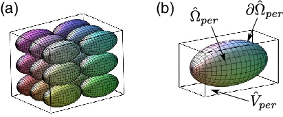
Charge transport in the electrolyte is described by the equations (2.60a)–(2.60c). At the interface with an electrode particle, the transfer current density is given by the Butler–Volmer relation (3.17) and this can be equated to the current flowing into the electrolyte via the boundary condition:
 \begin{eqnarray}\textbf{j} \cdot \textbf{N}|_{\partial \hat{\Omega}_{\mathrm{per}}} = j_{\rm tr} (\phi_{\rm s}-\varphi,c_{\rm s},c)|_{\partial \hat{\Omega}_{\mathrm{per}}}, \end{eqnarray}
where
 $\textbf{N}$
is the unit outward normal to the interface (it points into the electrolyte region). A boundary condition for (2.60a), the equation for conservation of lithium ions, is provided by noting that all charge transfer across this surface takes place via the motion of lithium ions. Hence, we have the following condition on
$\textbf{N}$
is the unit outward normal to the interface (it points into the electrolyte region). A boundary condition for (2.60a), the equation for conservation of lithium ions, is provided by noting that all charge transfer across this surface takes place via the motion of lithium ions. Hence, we have the following condition on
 $\textbf{q}_p$
, the flux of positively charged lithium ions:
$\textbf{q}_p$
, the flux of positively charged lithium ions:
 \begin{eqnarray}\textbf{q}_p\cdot \textbf{N}|_{\partial \hat{\Omega}_{\mathrm{per}}} = \frac{1}{F} j_{\rm tr}(\phi_{\rm s}-\varphi,c_{\rm s},c)|_{\partial \hat{\Omega}_{\mathrm{per}}}, \quad \mbox{where} \quad \textbf{q}_p=-{D_{\rm eff}}(c) \nabla c+\frac{t_{+}^{0}}{F} \textbf{j}. \end{eqnarray}
Note that (4.1) and (4.2) imply that the flux of negative ions is zero with
 $\textbf{q}_n\cdot \textbf{N}|_{\partial \hat{\Omega}_{\mathrm{per}}}=0$
, as required physically.
$\textbf{q}_n\cdot \textbf{N}|_{\partial \hat{\Omega}_{\mathrm{per}}}=0$
, as required physically.
In each individual electrode particle
 $\hat{\Omega}_{\mathrm{per}}$
, a diffusion equation is solved for lithium concentration in the AM. Generalising (3.2) to an arbitrary shaped particle and allowing for non-linear diffusion gives
$\hat{\Omega}_{\mathrm{per}}$
, a diffusion equation is solved for lithium concentration in the AM. Generalising (3.2) to an arbitrary shaped particle and allowing for non-linear diffusion gives
 \begin{eqnarray}\frac{\partial c_{\rm s}}{\partial t}= \nabla \cdot ( D_{\rm s}(c_{\rm s}) \nabla c_{\rm s}) \qquad \mbox{in} \quad \hat{\Omega}_{\mathrm{per}}, \end{eqnarray}
with boundary condition:
 \begin{eqnarray}-D_{\rm s}(c_{\rm s}) \nabla c_{\rm s} \cdot \textbf{N}|_{\partial \hat{\Omega}_{\mathrm{per}}}= \frac{1}{F} j_{\rm tr}(\phi_{\rm s}-\varphi,c_{\rm s},c)|_{\partial \hat{\Omega}_{\mathrm{per}}}. \end{eqnarray}
4.2 Homogenising the equations in a porous electrode
Here, we homogenise the moderately concentrated electrolyte equations (2.60a)–(2.60c), with boundary conditions (4.1)–(4.2), over a porous electrode formed by an array of electrode particles permeated by the electrolyte using the asymptotic method of multiple scales. We remark that volume averaging can also be used to obtain the same equations but that, in contrast to multiple scales which is systematic, volume averaging relies on ad hoc closure conditions. The interested reader is referred to [Reference Davit, Bell, Byrne, Chapman, Kimpton, Lang, Leonard, Oliver, Pearson, Shipley, Whiteley, Wood and Quintard21] for an in-depth comparison between the two techniques. In order to do this, we assume that the electrode can be subdivided into an array of cells over which the electrode structure is locally periodic; that is, the structure inside neighbouring cells is virtually identical but may differ significantly between cells separated on the macroscopic lengthscale.Footnote
4
An example of cell microstructure, around an array of ellipsoidal electrode particles, is illustrated in Figure 5. To average the problem using homogenisation, we introduce a variable
 $\hat{\textbf{x}}$
to indicate position in the microscopic cell and another variable
$\hat{\textbf{x}}$
to indicate position in the microscopic cell and another variable
 $\textbf{x}$
to indicate macroscopic position in the entire electrode. Since a very similar analysis has been conducted in [Reference Richardson, Denuault and Please80] for a dilute electrolyte, we omit the details of the analysis here and merely write down the results (in dimensional form). These consist of macroscopic equations for the lithium ion concentration c and the electrolyte potential (measured with respect to a lithium electrode)
$\textbf{x}$
to indicate macroscopic position in the entire electrode. Since a very similar analysis has been conducted in [Reference Richardson, Denuault and Please80] for a dilute electrolyte, we omit the details of the analysis here and merely write down the results (in dimensional form). These consist of macroscopic equations for the lithium ion concentration c and the electrolyte potential (measured with respect to a lithium electrode)
 $\varphi$
that are formulated in terms of the microscopically volume averaged lithium ion flux
$\varphi$
that are formulated in terms of the microscopically volume averaged lithium ion flux
 $\langle \textbf{q}_p \rangle$
, the microscopically volume averaged current density
$\langle \textbf{q}_p \rangle$
, the microscopically volume averaged current density
 $\langle \textbf{j} \rangle$
and the microscopically surface averaged transfer current density
$\langle \textbf{j} \rangle$
and the microscopically surface averaged transfer current density
 $\bar{j}_{\rm tr}$
. These averaged quantities are formally defined in terms of integrals over the microscopic cells as follows:
$\bar{j}_{\rm tr}$
. These averaged quantities are formally defined in terms of integrals over the microscopic cells as follows:
 \begin{eqnarray}\langle \textbf{j} \rangle=\frac{1}{|\hat{V}_{\mathrm{per}}|+|\hat{\Omega}_{\mathrm{per}}|} \int_{\hat{V}_{\mathrm{per}}} \textbf{j}\; {\rm d} \hat{V}, \qquad \langle \textbf{q}_p \rangle=\frac{1}{|\hat{V}_{\mathrm{per}}|+|\hat{\Omega}_{\mathrm{per}}|} \int_{\hat{V}_{\mathrm{per}}} \textbf{q}_p\; {\rm d} \hat{V}, \end{eqnarray}
 \begin{eqnarray} \bar{j}_{\rm tr}=\frac{1}{|S_{\partial \hat{\Omega}_{\mathrm{per}}}|} \int_{{\partial} \hat{\Omega}_{\mathrm{per}}} j_{{\rm tr}}\; {\rm d} \hat{S}, \end{eqnarray}
where the integrals are over the microscopic variable and the averaged functions depend only on the macroscopic space variable
 $\textbf{x}$
and time t. The quantities
$\textbf{x}$
and time t. The quantities
 $|\hat{V}_{\mathrm{per}}|(\textbf{x})$
,
$|\hat{V}_{\mathrm{per}}|(\textbf{x})$
,
 $|\hat{\Omega}_{\mathrm{per}}|(\textbf{x})$
and
$|\hat{\Omega}_{\mathrm{per}}|(\textbf{x})$
and
 $|S_{\partial \hat{\Omega}_{\mathrm{per}}}|(\textbf{x})$
are defined by:
$|S_{\partial \hat{\Omega}_{\mathrm{per}}}|(\textbf{x})$
are defined by:
 \begin{eqnarray}|\hat{V}_{\mathrm{per}}|= \int_{\hat{V}_{\mathrm{per}}} {\rm d} \hat{V}, \qquad |\hat{\Omega}_{\mathrm{per}}|=\int_{\hat{\Omega}_{\mathrm{per}}} {\rm d} \hat{V}, \qquad |S_{\partial \hat{\Omega}_{\mathrm{per}}}|=\int_{\partial \hat{\Omega}_{\mathrm{per}}} {\rm d} \hat{S},\end{eqnarray}
and respectively give the volume of electrolyte, the volume of electrode particle and the surface area of electrode particle in the microscopic cell. The macroscopic homogenised electrolyte equations then take the form:
 \begin{eqnarray}\epsilon_v \frac{\partial c}{\partial t} + \nabla \cdot \langle \textbf{q}_p \rangle= \frac{b_{et}}{F} \bar{j}_{\rm tr}, \qquad \langle \textbf{q}_p \rangle= -{D_{\rm eff}}(c) \underline{\underline{B}} \nabla c + \frac{t_{+}^{0}}{F} \langle \textbf{j} \rangle,\end{eqnarray}
 \begin{eqnarray}\nabla \cdot \langle \textbf{j} \rangle= b_{et} \bar{j}_{\rm tr}, \qquad \langle \textbf{j} \rangle=-\kappa(c) \underline{\underline{B}} \left( \nabla \varphi - 2 (1-t_{+}^{0}) \frac{RT}{F} { \frac{a'_{\!\!e}(c)}{a_e(c)}\nabla c }\right),\end{eqnarray}
where the final term in the current equation (4.7b) takes the standard form
 $2 (1-t_{+}^{0}) ({RT}/{F c}) \nabla c$
when the activity is that for an ideal solution (i.e.
$2 (1-t_{+}^{0}) ({RT}/{F c}) \nabla c$
when the activity is that for an ideal solution (i.e.
 $a_e(c)=c/c_T$
). It is interesting to note that the equations for the electrolyte after homogenisation, (4.7a)–(4.7b), are very similar in nature to the original equations for the pure electrolyte, (2.60a)–(2.60c), except that there are now source terms in the conservation equations corresponding to the transfer current from the electrodes. Here,
$a_e(c)=c/c_T$
). It is interesting to note that the equations for the electrolyte after homogenisation, (4.7a)–(4.7b), are very similar in nature to the original equations for the pure electrolyte, (2.60a)–(2.60c), except that there are now source terms in the conservation equations corresponding to the transfer current from the electrodes. Here,
 $\epsilon_v$
is the volume fraction of the electrolyte defined by:
$\epsilon_v$
is the volume fraction of the electrolyte defined by:
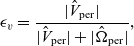 \begin{eqnarray*}\epsilon_v= \frac{|\hat{V}_{\mathrm{per}}|}{|\hat{V}_{\mathrm{per}}|+|\hat{\Omega}_{\mathrm{per}}|},\end{eqnarray*}
the Brunauer–Emmett–Teller surface area (BET surface area),
 $b_{et}$
, that is, the surface area of particles per unit volume of electrode, is defined by:
$b_{et}$
, that is, the surface area of particles per unit volume of electrode, is defined by:
 \begin{eqnarray*}b_{et}= \frac{\int_{\hat{\Omega}_{\text{per}}} {\rm d}S}{|\hat{V}_{\mathrm{per}}|+|\hat{\Omega}_{\mathrm{per}}|},\end{eqnarray*}
and
 $\underline{\underline{B}}$
is the dimensionless permeability tensor whose nine components are defined by the relations:
$\underline{\underline{B}}$
is the dimensionless permeability tensor whose nine components are defined by the relations:
 \begin{eqnarray}B_{ij} = \frac{1}{|\hat{V}_{\mathrm{per}}|+|\hat{\Omega}_{\mathrm{per}}|} \int_{\hat{V}_{\mathrm{per}}} \left( \delta_{ij} - \frac{\partial \chi^{(j)}}{\partial x_i} \right) {\rm d} \hat{V} \quad\mbox{for} \quad i=1,2,3 \mbox{ and } j=1,2,3, \end{eqnarray}
in which the three characteristic functions
 $\chi^{(j)}$
(
$\chi^{(j)}$
(
 $j=1,2,3$
) are solutions to the local cell problems:
$j=1,2,3$
) are solutions to the local cell problems:
 \begin{eqnarray} \left. \begin{array}{c} \hat{\nabla}^2 \chi^{(j)}=0 \quad \mbox{in} \quad \hat{V}_{\mathrm{per}}, \\[5pt] \hat{\nabla} \chi^{(j)} \cdot \textbf{n} |_{\partial \hat{\Omega}_{\mathrm{per}} }= \textbf{e}_j \cdot \textbf{n} |_{\partial \hat{\Omega}_{\mathrm{per}} }, \\[5pt] \chi^{(j)} \quad \mbox{periodic in $\hat{x}$ on} \quad \hat{V}_{\mathrm{per}}, \\[5pt] \int_{\hat{V}_{\mathrm{per}}} \chi^{(j)}\; {\rm d} \hat{V}=0 \end{array} \right\} \quad \mbox{for} \quad i=1,2,3,\end{eqnarray}
where
 $\textbf{e}_j$
is a basis vector in the
$\textbf{e}_j$
is a basis vector in the
 $\hat{x}_j$
-direction and
$\hat{x}_j$
-direction and
 $\textbf{n}$
is the unit outward normal (pointing from
$\textbf{n}$
is the unit outward normal (pointing from
 $\hat{\Omega}_{\mathrm{per}}$
into
$\hat{\Omega}_{\mathrm{per}}$
into
 $\hat{V}_{\mathrm{per}}$
) to the surface
$\hat{V}_{\mathrm{per}}$
) to the surface
 $\partial \hat{\Omega}_{\mathrm{per}}$
.
$\partial \hat{\Omega}_{\mathrm{per}}$
.
We note also here the possibility of using this type of homogenisation technique in conjunction with microscale three-dimensional image data obtained from real battery electrodes in order to obtain more realistic representations of the geometric parameters
 $\epsilon_v$
,
$\epsilon_v$
,
 $B_{ij}$
and
$B_{ij}$
and
 $b_{et}$
, as discussed for example in [Reference Cooper, Bertei, Shearing, Kilner and Brandon17, Reference Foster, Gully, Liu, Krachkovskiy, Wu, Schougaard, Jiang, Goward, Botton and Protas35, Reference Gully, Liu, Srinivasan, Sethurajan, Schougaard and Protas41]. In many papers, the tensor
$b_{et}$
, as discussed for example in [Reference Cooper, Bertei, Shearing, Kilner and Brandon17, Reference Foster, Gully, Liu, Krachkovskiy, Wu, Schougaard, Jiang, Goward, Botton and Protas35, Reference Gully, Liu, Srinivasan, Sethurajan, Schougaard and Protas41]. In many papers, the tensor
 $\underline{\underline{B}}$
is taken to be a constant times the unit tensor, which correspond to a highly symmetric set of particles, such as spherical particles on a regular lattice, and proves to be quite a reasonable model.
$\underline{\underline{B}}$
is taken to be a constant times the unit tensor, which correspond to a highly symmetric set of particles, such as spherical particles on a regular lattice, and proves to be quite a reasonable model.
The homogenised electrolyte equations (4.7a)–(4.7b) must be solved in conjunction with the macroscopic equations for the current flow through the solid part of the electrode. These can be obtained by using a constitutive law for current flow in the electrode matrix (3.1) with a current conservation equation that accounts for transfer of charge from the electrode matrix into the electrolyte:
 \begin{eqnarray}\nabla \cdot \textbf{j}_{\rm s}= -b_{et} \bar{j}_{\rm tr}, \quad \mbox{where} \quad \textbf{j}_{\rm s}= -\kappa_{\rm s} \nabla \phi_{\rm s}. \end{eqnarray}
The system of macroscopic equations (4.7a)–(4.7b) and (4.10) require to be solved along with the microscopic lithium transport equations (4.3) and (4.4), at each point in macroscopic space, in order to determine
 $c_{\rm s}|_{\partial \hat{\Omega}_{\mathrm{per}}}$
, which is required to obtain the transfer current
$c_{\rm s}|_{\partial \hat{\Omega}_{\mathrm{per}}}$
, which is required to obtain the transfer current
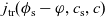 $j_{\rm tr}(\phi_{\rm s}-\varphi,c_{\rm s},c)$
(and hence
$j_{\rm tr}(\phi_{\rm s}-\varphi,c_{\rm s},c)$
(and hence
 $\bar{j}_{\rm tr}$
as given in (4.5b)).
$\bar{j}_{\rm tr}$
as given in (4.5b)).
Note that where the electrode particles are spherical (and isotropic),
 $c_{\rm s}|_{\partial \hat{\Omega}_{\mathrm{per}}}$
is uniform over the particle surface and is thus just a function of the macroscopic variables. It follows therefore that
$c_{\rm s}|_{\partial \hat{\Omega}_{\mathrm{per}}}$
is uniform over the particle surface and is thus just a function of the macroscopic variables. It follows therefore that
 $j_{\rm tr}$
is also just a function of the macroscopic variables and, as a consequence of the averaging equation (4.5b) it follows that
$j_{\rm tr}$
is also just a function of the macroscopic variables and, as a consequence of the averaging equation (4.5b) it follows that
 \begin{eqnarray}\bar{j}_{\rm tr}=j_{\rm tr} \quad \mbox{for spherically symmetric electrode particles.} \end{eqnarray}
4.2.1 Remarks on the role of binder
In the discussion above, we have assumed that the electrode was formed solely from electrode particles bathed in electrolyte. While this is often a reasonable description of research cells, many commercial devices also incorporate a significant volume fraction of polymer binder material that acts both to enhance the structural integrity of the device and, in combination with a conductivity enhancer (such as carbon black), maintain good electrical contact between electrode particles (these are often poor conductors). Three-dimensional images of typical commercial electrodes using focused ion beam in combination with scanning electron microscopy (FIB-SEM) can be found in [Reference Foster, Gully, Liu, Krachkovskiy, Wu, Schougaard, Jiang, Goward, Botton and Protas35, Reference Gully, Liu, Srinivasan, Sethurajan, Schougaard and Protas41, Reference Liu, Foster, Gully, Krachkovskiy, Jiang, Wu, Yang, Protas, Goward and Botton60]. These show a porous binder material filling almost all the space between electrode particles with the exception of some linear features around the electrode particles where it appears that the binder has become delaminated from the electrode particles.Footnote
5
The porosity and pore size of the binder materials vary significantly between different electrode types. Typical pore sizes are usually in the range 10–500 nm, much smaller than typical electrode particle sizes which are usually at least micron sized. To account for these effects within an homogenisation approach, the analysis could be modified in two possible ways. Firstly, it could be performed directly on a microstructure in which all three constituents (electrode particle, electrolyte and binder) are resolved by the cell problem and would follow a very similar pattern to that described above in which the binder was treated as part of
 $\hat{\Omega}_{\mathrm{per}}$
with an interface with the electrolyte on which the transfer current density
$\hat{\Omega}_{\mathrm{per}}$
with an interface with the electrolyte on which the transfer current density
 $j_{\rm tr} \equiv 0$
. Secondly, because obtaining a good representation of the pore geometry in the binder is challenging, even using modern high-performance microscopy, see [Reference Liu, Foster, Gully, Krachkovskiy, Jiang, Wu, Yang, Protas, Goward and Botton60], it is probably better to treat the electrolyte-permeated nanoporous binder as a single electrolyte material (albeit it one with reduced electrolyte volume fraction, electrolyte diffusivity and conductivity) and homogenise over the electrode particles and this composite material. Indeed this second approach is a standard way of treating such two phase (electrolyte/binder) materials in the literature which are often termed porous solid polymer electrolytes (see, e.g. [Reference Miao, Liu, Zhu, Liu, Li, Wang and Li66]).
$j_{\rm tr} \equiv 0$
. Secondly, because obtaining a good representation of the pore geometry in the binder is challenging, even using modern high-performance microscopy, see [Reference Liu, Foster, Gully, Krachkovskiy, Jiang, Wu, Yang, Protas, Goward and Botton60], it is probably better to treat the electrolyte-permeated nanoporous binder as a single electrolyte material (albeit it one with reduced electrolyte volume fraction, electrolyte diffusivity and conductivity) and homogenise over the electrode particles and this composite material. Indeed this second approach is a standard way of treating such two phase (electrolyte/binder) materials in the literature which are often termed porous solid polymer electrolytes (see, e.g. [Reference Miao, Liu, Zhu, Liu, Li, Wang and Li66]).
4.2.2 Practical application of homogenisation
There are several important practical results that arise from this homogenisation procedure. Firstly, we learn that the same dimensionless permeability tensor appears in equation (4.7a) for the averaged ion flux
 $\langle \textbf{q}_p \rangle$
as appears in that for
$\langle \textbf{q}_p \rangle$
as appears in that for
 $\langle \textbf{j} \rangle$
, the averaged current (4.7b). Secondly, it is apparent that definition of the dimensionless permeability tensor
$\langle \textbf{j} \rangle$
, the averaged current (4.7b). Secondly, it is apparent that definition of the dimensionless permeability tensor
 $\underline{\underline{B}}$
, contained in (4.8) and (4.9), is equivalent to that which would be calculated in the homogenisation of Laplace’s equation:
$\underline{\underline{B}}$
, contained in (4.8) and (4.9), is equivalent to that which would be calculated in the homogenisation of Laplace’s equation:
 \begin{eqnarray}\nabla^2 c =0 \quad \mbox{in} \quad \hat{V}_{\mathrm{per}}, \quad \nabla c \cdot \textbf{n}|_{\partial \hat{V}_{\mathrm{per}}}=0, \end{eqnarray}
over the same domain
 $\hat{V}_{\mathrm{per}}$
. Indeed homogenising (4.12) results in the averaged equations:
$\hat{V}_{\mathrm{per}}$
. Indeed homogenising (4.12) results in the averaged equations:
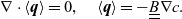 \begin{eqnarray}\nabla \cdot \langle \textbf{q} \rangle=0, \quad \langle \textbf{q} \rangle =- \underline{\underline{B}} \nabla c.\end{eqnarray}
Thus, from a practical perspective, the computation of the dimensionless permeability tensor
 $\underline{\underline{B}}$
can be accomplished by solving Laplace’s equation over a representative cell domain,
$\underline{\underline{B}}$
can be accomplished by solving Laplace’s equation over a representative cell domain,
 $\hat{V}_{\mathrm{per}}$
, culled from real image data, and computing the averaged flux
$\hat{V}_{\mathrm{per}}$
, culled from real image data, and computing the averaged flux
 $\langle \textbf{q} \rangle$
that passes through this cell in response to a unit differences in concentration across the faces of the cell. This is the approach that has been adopted in a number of works, including [Reference Gully, Liu, Srinivasan, Sethurajan, Schougaard and Protas41, Reference Le Houx and Kramer57, Reference Le Houx, Osenberg, Neumann, Binder, Schmidt, Manke, Carraro and Kramer58, Reference Liu, Foster, Gully, Krachkovskiy, Jiang, Wu, Yang, Protas, Goward and Botton60, Reference Tjaden, Cooper, Brett, Kramer and Shearing96].
$\langle \textbf{q} \rangle$
that passes through this cell in response to a unit differences in concentration across the faces of the cell. This is the approach that has been adopted in a number of works, including [Reference Gully, Liu, Srinivasan, Sethurajan, Schougaard and Protas41, Reference Le Houx and Kramer57, Reference Le Houx, Osenberg, Neumann, Binder, Schmidt, Manke, Carraro and Kramer58, Reference Liu, Foster, Gully, Krachkovskiy, Jiang, Wu, Yang, Protas, Goward and Botton60, Reference Tjaden, Cooper, Brett, Kramer and Shearing96].
Bruggeman Relation.
For isotropic materials, for which
 $(\underline{\underline{B}})_{ij}={\mathcal B} \delta_{ij}$
where
$(\underline{\underline{B}})_{ij}={\mathcal B} \delta_{ij}$
where
 $ \delta_{ij}$
is the Kronecker delta tensor, a simple, but entirely ad hoc, way of computing the dimensionless permeability factor
$ \delta_{ij}$
is the Kronecker delta tensor, a simple, but entirely ad hoc, way of computing the dimensionless permeability factor
 ${\mathcal B}$
is provided by Bruggeman relation, [Reference Bruggeman13], which states that
${\mathcal B}$
is provided by Bruggeman relation, [Reference Bruggeman13], which states that
 \begin{eqnarray*}{\mathcal B}(x)=(\epsilon_v(x))^{1.5}.\end{eqnarray*}
where
 $\epsilon_v$
is the electrolyte volume fraction.
$\epsilon_v$
is the electrolyte volume fraction.
4.3 The Newman or pseudo-2d model
As mentioned previously, a common approach in the literature to modelling practical batteries is to use the so-called Newman or pseudo-2d model where the behaviour on the macroscale is one-dimensional (with spatial position denoted by x) and transport of lithium on the microscale takes place within spherical particles and is thus also one-dimensional taking place in the particles’ radial direction (with radial position denoted by r). These assumptions are tantamount to assuming that the averaged macroscopic vector-valued currents and fluxes from Sections 4.1 to 4.2 are only non-zero in the x-direction. Henceforth, we will replace these vector quantities with scalar counterparts. Here, we describe the system of equations that arise for such a situation exploiting the homogenisation results described previously in (4.7a)–(4.10) and including the typical units.
As alluded to above, x denotes position across the cell in the direction perpendicular to the current collectors which are positioned at
 $x=L_1$
and
$x=L_1$
and
 $x=L_4$
, respectively so that
$x=L_4$
, respectively so that
 $x \in (L_1,L_4)$
. The cell is subdivided into three regions (as illustrated in Figure 1) with the negative electrode occupying the region
$x \in (L_1,L_4)$
. The cell is subdivided into three regions (as illustrated in Figure 1) with the negative electrode occupying the region
 $x \in (L_1,L_{2})$
, the separator occupying the region
$x \in (L_1,L_{2})$
, the separator occupying the region
 $x \in (L_2,L_3)$
and the positive electrode occupying the region
$x \in (L_2,L_3)$
and the positive electrode occupying the region
 $x\in (L_3,L_4)$
. In the electrolyte, which permeates the whole cell (i.e.
$x\in (L_3,L_4)$
. In the electrolyte, which permeates the whole cell (i.e.
 $x\in (L_1,L_4)$
), we seek to determine the Li-ion concentration c(x,t) (mol m−3), the electric potential (measured with respect to a reference lithium electrode)
$x\in (L_1,L_4)$
), we seek to determine the Li-ion concentration c(x,t) (mol m−3), the electric potential (measured with respect to a reference lithium electrode)
 $\varphi (x,t)$
(V) and the ionic current density
$\varphi (x,t)$
(V) and the ionic current density
 $\langle j \rangle(x,t)$
(A m−2). In the negative electrode (
$\langle j \rangle(x,t)$
(A m−2). In the negative electrode (
 $x \in (L_1,L_2)$
), we seek solutions for the solid phase potential
$x \in (L_1,L_2)$
), we seek solutions for the solid phase potential
 $\phi_{\rm s}^{(\rm a)}(x,t)$
and the solid phase current
$\phi_{\rm s}^{(\rm a)}(x,t)$
and the solid phase current
 $j_{\rm s}^{(\rm a)}(x,t)$
. In addition, we seek to determine the lithium distribution
$j_{\rm s}^{(\rm a)}(x,t)$
. In addition, we seek to determine the lithium distribution
 $c_{\rm s}^{(\rm a)}(r,x,t)$
within the (negative) electrode particles (of radius
$c_{\rm s}^{(\rm a)}(r,x,t)$
within the (negative) electrode particles (of radius
 $R^{(\rm a)}(x)$
) as a function of position
$R^{(\rm a)}(x)$
) as a function of position
 $r \in [0,R^{(\rm a)}(x)]$
within the particle and the position x of the particle across the electrode width. Similarly in the positive electrode (
$r \in [0,R^{(\rm a)}(x)]$
within the particle and the position x of the particle across the electrode width. Similarly in the positive electrode (
 $x \in (L_3,L_4)$
), we seek solutions for the solid phase potential
$x \in (L_3,L_4)$
), we seek solutions for the solid phase potential
 $\phi_{\rm s}^{(\rm c)}(x,t)$
, the solid phase current
$\phi_{\rm s}^{(\rm c)}(x,t)$
, the solid phase current
 $j_{\rm s}^{(\rm c)}(x,t)$
and also the lithium distribution
$j_{\rm s}^{(\rm c)}(x,t)$
and also the lithium distribution
 $c_{\rm s}^{(\rm c)}(r,x,t)$
within the (positive) electrode particles (of radius
$c_{\rm s}^{(\rm c)}(r,x,t)$
within the (positive) electrode particles (of radius
 $R^{(\rm c)}(x)$
) as a function both of position
$R^{(\rm c)}(x)$
) as a function both of position
 $r\in [0,R^{(\rm c)}(x)]$
within the particle and the position x of the particle within the electrode. A sketch of the device geometry as well as an illustration of the domains of definition of the dependent variables is shown in Figure 1. Throughout what follows, we assume that the transport of lithium within both negative and positive electrode particles occurs through non-linear isotropic diffusion, though as discussed in Section 3.2 this is not the only possibility. Furthermore, since the electrode particles are spherical we can make use of the simplification (4.11) in order to write
$r\in [0,R^{(\rm c)}(x)]$
within the particle and the position x of the particle within the electrode. A sketch of the device geometry as well as an illustration of the domains of definition of the dependent variables is shown in Figure 1. Throughout what follows, we assume that the transport of lithium within both negative and positive electrode particles occurs through non-linear isotropic diffusion, though as discussed in Section 3.2 this is not the only possibility. Furthermore, since the electrode particles are spherical we can make use of the simplification (4.11) in order to write
 $\bar{j}_{\rm tr}=j_{\rm tr}$
. The assumptions that the particles are spherical and that their radii vary slowly, that is, that their size depends on macroscopic position but neighbouring particles are almost the same size, gives rise to the following relationships:
$\bar{j}_{\rm tr}=j_{\rm tr}$
. The assumptions that the particles are spherical and that their radii vary slowly, that is, that their size depends on macroscopic position but neighbouring particles are almost the same size, gives rise to the following relationships:
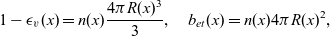 \begin{eqnarray} 1-\epsilon_v(x) = n(x) \frac{4 \pi R(x)^3}{3}, \quad b_{et}(x)=n(x) 4 \pi R(x)^2,\end{eqnarray}
where n(x) is the number density of electrode particles and, owing to our assumption that volume fraction of binder is negligible,
 $1-\epsilon_v$
is the volume fraction of electrode particles.
$1-\epsilon_v$
is the volume fraction of electrode particles.
The pseudo-2d model, which follows from the homogenisation described in Section 4.2 and describes the performance of a cell at constant temperature, is now stated in full in equations (4.15)–(4.22c). In this model, we denote variables and parameters relating to the negative electrode (or anode) by the superscript (a) and variables and parameters relating to the positive electrode (or cathode) by the superscript (c). The transport equations for the electrolyte, obtained from (4.7a) to (4.7b), are
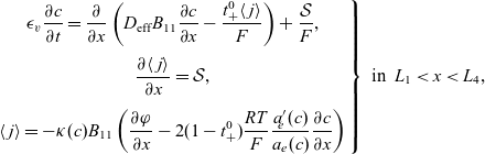 \begin{eqnarray}\left. \begin{array}{c}\displaystyle \epsilon_v \frac{\partial c}{\partial t}= \frac{\partial}{\partial x} \left({D_{\rm eff}} B_{11} \frac{\partial c}{\partial x} - \frac{t_{+}^{0} \langle \,j \rangle}{F} \right) + \frac{\mathcal{S}}{F},\\ \displaystyle \frac{\partial \langle \,j \rangle}{\partial x} = \mathcal{S}, \\ \displaystyle \langle \,j \rangle=-\kappa(c) B_{11} \left( \frac{\partial \varphi}{\partial x} - 2 (1-t_{+}^{0}) \frac{RT}{F} { \frac{a'_{\!\!e}(c)}{a_e(c)} \frac{\partial c}{\partial x} }\right)\end{array} \right\} \ \mbox{in} \ \ L_1<x<L_4, \end{eqnarray}
where the volumetric current source term
 $\mathcal{S}(x,t)$
is given by:
$\mathcal{S}(x,t)$
is given by:
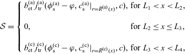 \begin{eqnarray}\mathcal{S}= \left\{ \begin{array}{lll} \displaystyle b_{\rm et}^{(\rm a)} j_{\rm tr}^{(\rm a)}(\phi_{\rm s}^{(\rm a)}-\varphi,c_{\rm s}^{(\rm a)}|_{r=R^{(\rm a)}(x)},c), & \mbox{for} & L_1<x<L_2, \\ 0, & \mbox{for} & L_2\leq x \leq L_3,\\ \displaystyle b_{\rm et}^{(\rm c)} j_{\rm tr}^{(\rm c)}(\phi_{\rm s}^{(\rm c)}-\varphi,c_{\rm s}^{(\rm c)}|_{r=R^{(\rm c)}(x)},c), & \mbox{for} & L_3<x<L_4,\end{array} \right. \end{eqnarray}
and where the electrolyte volume fraction
 $\epsilon_v$
and the
$\epsilon_v$
and the
 $B_{11}$
component of the permeability tensor are evaluated appropriately in each of the three regions. As discussed in Section 4.2,
$B_{11}$
component of the permeability tensor are evaluated appropriately in each of the three regions. As discussed in Section 4.2,
 $B_{11}$
can be computed by solving the appropriate cell problems. However, a common approach is to instead estimate its value using
$B_{11}$
can be computed by solving the appropriate cell problems. However, a common approach is to instead estimate its value using
 $B_{11}= \epsilon_v^p$
where p is the Bruggeman porosity exponent (a non-dimensional constant), which is commonly taken to be
$B_{11}= \epsilon_v^p$
where p is the Bruggeman porosity exponent (a non-dimensional constant), which is commonly taken to be
 $p=1.5$
, see [Reference Bruggeman13, Reference Gully, Liu, Srinivasan, Sethurajan, Schougaard and Protas41, Reference Gupta, Seo, Zhang, Du, Sastry and Shyy42]. We note also the work of [Reference Shen and Chen86] who discuss some alternative estimation methods beyond the Bruggeman approximation. Boundary conditions on the electrolyte equations are enforced by the requirements that there is no flow of electrolyte current or flux of lithium ions into the current collectors at
$p=1.5$
, see [Reference Bruggeman13, Reference Gully, Liu, Srinivasan, Sethurajan, Schougaard and Protas41, Reference Gupta, Seo, Zhang, Du, Sastry and Shyy42]. We note also the work of [Reference Shen and Chen86] who discuss some alternative estimation methods beyond the Bruggeman approximation. Boundary conditions on the electrolyte equations are enforced by the requirements that there is no flow of electrolyte current or flux of lithium ions into the current collectors at
 $x=L_1$
and
$x=L_1$
and
 $x=L_4$
and are
$x=L_4$
and are
 \begin{eqnarray}\begin{array}{cc}\langle \,j \rangle|_{x=L_1}=0, & \displaystyle \left. \frac{\partial c}{\partial x} \right|_{x=L_1}=0, \\ \langle \,j \rangle|_{x=L_4}=0, & \displaystyle \left. \frac{\partial c}{\partial x} \right|_{x=L_4}=0.\end{array} \end{eqnarray}
In the negative electrode matrix conservation of current and Ohm’s Law, as given by (4.10), are described by:
 \begin{eqnarray}\frac{\partial j_{\rm s}^{(\rm a)}}{\partial x}= - \mathcal{S}, \ \ \mbox{and} \ \ j_{\rm s}^{(\rm a)}=-\kappa_{\rm s}^{(\rm a)} \frac{\partial \phi_{\rm s}^{(\rm a)}}{\partial x}, \quad \mbox{in} \ \ L_1<x<L_2, \end{eqnarray}
and are supplemented by a boundary condition at the interface with the current collector, which specifies the current inflow, and one at the interface with the insulating separator into which the current in the matrix does not flow
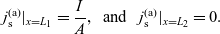 \begin{eqnarray}j_{\rm s}^{(\rm a)}|_{x=L_1}=\frac{I}{A}, \ \ \mbox{and} \ \ \ j_{\rm s}^{(\rm a)}|_{x=L_2}=0. \end{eqnarray}
Here, I is the current flowing into the cell and A is the cell’s area. In the same region, lithium transport (as described in (4.3)–(4.4)) within the spherical anode particles satisfies the problem:
 \begin{eqnarray}\frac{\partial c_{\rm s}^{(\rm a)}}{\partial t} = \frac{1}{r^2} \frac{\partial}{\partial r} \left( r^2 D_{\rm s}^{(\rm a)}( c_{\rm s}^{(\rm a)}) \frac{\partial c_{\rm s}^{(\rm a)} }{\partial r} \right) \quad \mbox{for} \quad\left\{\begin{array}{c} 0\leqslant r < R^{(\rm a)}(x)\\ L_1<x<L_2 \end{array} \right., \end{eqnarray}
 \begin{eqnarray} c_{\rm s}^{(\rm a)} \ \ \mbox{bounded on} \ \ r=0, \end{eqnarray}
 \begin{eqnarray}\left. D_{\rm s}^{(\rm a)}( c_{\rm s}^{(\rm a)}) \frac{\partial c_{\rm s}^{(\rm a)} }{\partial r} \right|_{r=R^{(\rm a)}(x)} =-\frac{j_{\rm tr}^{(\rm a)}(\phi_{\rm s}^{(\rm a)}-\varphi,c_{\rm s}^{(\rm a)}|_{r=R^{(\rm a)}(x)},c)}{F}. \end{eqnarray}
In the positive electrode (or cathode), an analogous set of equations and boundary conditions describe the current flow and transport of lithium within the cathode particles. They are
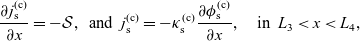 \begin{eqnarray}\frac{\partial j_{\rm s}^{(\rm c)}}{\partial x}= - \mathcal{S}, \ \ \mbox{and} \ \ j_{\rm s}^{(\rm c)}=-\kappa_{\rm s}^{(\rm c)} \frac{\partial \phi_{\rm s}^{(\rm c)}}{\partial x}, \quad \mbox{in} \ \ L_3<x<L_4, \end{eqnarray}
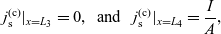 \begin{eqnarray}j_{\rm s}^{(\rm c)}|_{x=L_3}=0, \ \ \mbox{and} \ \ \ j_{\rm s}^{(\rm c)}|_{x=L_4}=\frac{I}{A}, \end{eqnarray}
with lithium transport within the spherical cathode particles being described by:
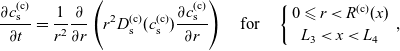 \begin{eqnarray}\frac{\partial c_{\rm s}^{(\rm c)}}{\partial t} = \frac{1}{r^2} \frac{\partial}{\partial r} \left( r^2 D_{\rm s}^{(\rm c)}( c_{\rm s}^{(\rm c)}) \frac{\partial c_{\rm s}^{(\rm c)} }{\partial r} \right) \quad \mbox{for} \quad \left\{\begin{array}{c} 0\leqslant r < R^{(\rm c)}(x)\\ L_3<x<L_4 \end{array} \right., \end{eqnarray}
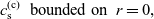 \begin{eqnarray} c_{\rm s}^{(\rm c)} \ \ \mbox{bounded on} \ \ r=0, \end{eqnarray}
 \begin{eqnarray}\left. D_{\rm s}^{(\rm c)}( c_{\rm s}^{(\rm c)}) \frac{\partial c_{\rm s}^{(\rm c)} }{\partial r} \right|_{r=R^{(\rm c)}(x)} =-\frac{j_{\rm tr}^{(\rm c)}(\phi_{\rm s}^{(\rm c)}-\varphi,c_{\rm s}^{(\rm c)}|_{r=R^{(\rm c)}(x)},c)}{F}. \end{eqnarray}
The transfer currents densities
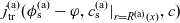 $j_{\rm tr}^{(\rm a)}(\phi_{\rm s}^{(\rm a)}-\varphi,c_{\rm s}^{(\rm a)}|_{r=R^{(\rm a)}(x)},c)$
and
$j_{\rm tr}^{(\rm a)}(\phi_{\rm s}^{(\rm a)}-\varphi,c_{\rm s}^{(\rm a)}|_{r=R^{(\rm a)}(x)},c)$
and
 $j_{\rm tr}^{(\rm c)}(\phi_{\rm s}^{(\rm c)}-\varphi,c_{\rm s}^{(\rm c)}|_{r=R^{(\rm c)}(x)},c)$
that describe the flow of current out of the anode and cathode particles, respectively, and which act to couple together the lithium transport problems in the electrolyte to those in the electrode particles are typically determined by the Butler–Volmer condition as discussed in Section 3.1.2. The existence and uniqueness of solution of the system (4.15)–(4.22c) have been proved in [Reference Díaz, Gómez-Castro and Ramos22]. We point out that, in some works in the literature (see, for instance [Reference Kim, Smith, Ireland and Pesaran51, Reference Smith88–Reference Smith and Wang90]), authors present incorrect boundary conditionsFootnote
6
at
$j_{\rm tr}^{(\rm c)}(\phi_{\rm s}^{(\rm c)}-\varphi,c_{\rm s}^{(\rm c)}|_{r=R^{(\rm c)}(x)},c)$
that describe the flow of current out of the anode and cathode particles, respectively, and which act to couple together the lithium transport problems in the electrolyte to those in the electrode particles are typically determined by the Butler–Volmer condition as discussed in Section 3.1.2. The existence and uniqueness of solution of the system (4.15)–(4.22c) have been proved in [Reference Díaz, Gómez-Castro and Ramos22]. We point out that, in some works in the literature (see, for instance [Reference Kim, Smith, Ireland and Pesaran51, Reference Smith88–Reference Smith and Wang90]), authors present incorrect boundary conditionsFootnote
6
at
 $x=L_1$
and
$x=L_1$
and
 $x=L_4$
. We note in passing that if these incorrect conditions are used, then it can be proved (see [Reference Ramos76]) that the corresponding system of boundary value problems does not have any solution unless
$x=L_4$
. We note in passing that if these incorrect conditions are used, then it can be proved (see [Reference Ramos76]) that the corresponding system of boundary value problems does not have any solution unless
 $I(t) \equiv 0$
.
$I(t) \equiv 0$
.
Once the model described above has been solved, we can estimate the state of the charge of the negative electrode SOC
 $^{(a)}(t)$
and of the positive electrode SOC
$^{(a)}(t)$
and of the positive electrode SOC
 $^{(c)}(t)$
, and the cell voltage V(t), at time t, by computing
$^{(c)}(t)$
, and the cell voltage V(t), at time t, by computing
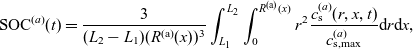 \begin{equation}\mbox{SOC}^{(a)}(t)=\frac{3}{(L_2-L_1)(R^{(\rm a)}(x))^3} \int_{L_1}^{L_2}\int_0^{R^{(\rm a)}(x)} r^2 \frac{c^{(a)}_{\rm s}(r,x,t)}{c^{(a)}_{\rm s,max}}{\rm d}r{\rm d}x,\end{equation}
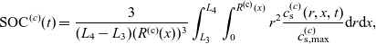 \begin{equation}\mbox{SOC}^{(c)}(t)=\frac{3}{(L_4-L_3)(R^{(\rm c)}(x))^3} \int_{L_3}^{L_4} \int_0^{R^{(\rm c)}(x)} r^2 \frac{c^{(c)}_{\rm s}(r,x,t)}{c^{(c)}_{\rm s,max}}{\rm d}r{\rm d}x,\end{equation}
 \begin{equation}V(t) = \phi_{\rm s} (L_4,t) - \phi_{\rm s} (L_1,t) - \frac{R_{\rm f}}{A}I(t),\end{equation}
where there is a constant resistance
 $R_{\rm f}$
which accounts for the potential dropped in the current collectors, but we remark that this is often negligible in practice. We note some ambiguity about how the state of charge of an electrode or cell should be defined. The definition given here might be referred to as the state of charge measured with respect to the theoretical maximum capacity. In the experimental literature, it is common to define the state of charge with reference to the capacity measured from a cell under a low-rate (dis)charge, see e.g. [Reference Barai, Widanage, Marco, McGordon and Jennings5, Reference Johns, Roberts, Wakizaka, Sanders and Owen46].
$R_{\rm f}$
which accounts for the potential dropped in the current collectors, but we remark that this is often negligible in practice. We note some ambiguity about how the state of charge of an electrode or cell should be defined. The definition given here might be referred to as the state of charge measured with respect to the theoretical maximum capacity. In the experimental literature, it is common to define the state of charge with reference to the capacity measured from a cell under a low-rate (dis)charge, see e.g. [Reference Barai, Widanage, Marco, McGordon and Jennings5, Reference Johns, Roberts, Wakizaka, Sanders and Owen46].
5 Example results of the model
To illustrate the capabilities of the model multiscale model, (4.15)–(4.22c), described in Section 4.3, we have applied it to model the discharge, and immediate subsequent recharge, of a Li
 $_x C_6$
graphite anode against an Li
$_x C_6$
graphite anode against an Li
 $_x$
(Ni
$_x$
(Ni
 $_{0.4}$
Co
$_{0.4}$
Co
 $_{0.6}$
)O
$_{0.6}$
)O
 $_2$
LNC cathode which are connected via a 1M LiPF
$_2$
LNC cathode which are connected via a 1M LiPF
 $_6$
in EC:DMC electrolyte. The parameterisation used here is closely based on that given in [Reference Ecker, Käbitz, Laresgoiti and Sauer29, Reference Ecker, Tran, Dechent, Käbitz, Warnecke and Sauer30] where a series of experiments were conducted on a high-energy pouch cell produced by Kokam; the values used here are summarised in Table 1.
$_6$
in EC:DMC electrolyte. The parameterisation used here is closely based on that given in [Reference Ecker, Käbitz, Laresgoiti and Sauer29, Reference Ecker, Tran, Dechent, Käbitz, Warnecke and Sauer30] where a series of experiments were conducted on a high-energy pouch cell produced by Kokam; the values used here are summarised in Table 1.
The parameter values used to carry out the simulations shown in Section 5. These are largely based on the work of [Reference Ecker, Käbitz, Laresgoiti and Sauer29, Reference Ecker, Tran, Dechent, Käbitz, Warnecke and Sauer30]. The functions used for the electrode conductivities were fitted to data in [Reference Ecker, Käbitz, Laresgoiti and Sauer29, Reference Ecker, Tran, Dechent, Käbitz, Warnecke and Sauer30] and the functions themselves are given in [Reference Korotkin, Sahu, O'Kane, Richardson and Foster54]

Figure 6 shows the discharge curve, and internal concentration and potential profiles during a relatively low-rate usage where a current demand of 0.13 A is applied for 4000 s and the cell is the immediately recharged at the same rate until it reaches a cut-off voltage of 4.2 V. We observe that under these conditions, concentration and potential gradients in the electrolyte are relatively modest. Likewise, the concentration is through the radius of the electrode particles is almost uniform; a consequence of the relatively large diffusivity in LNC. The largest gradients are observed internal to the anode particles and although these are not large enough to hamper the initial discharge, it is the inability of the graphite to transport intercalated Li from its surface into its interior that ultimately causes the recharging process to be interupted. At the final snapshot in time in panel (d), we observe that the concentration on the surface of the graphite particle has reached its maximum and therefore intercalation cannot proceed further at this location despite their being available space to accomodate Li in the particle’s interior.
Discharge (solid curves) and subsequent recharge (dashed curves) of a graphite-LNC cell bathed in 1M LiPF
 $_6$
electrolyte at a relatively low rate of 0.13 A. The full parameterisation is give in Table 1. Thick curves indiciate profiles at the beginning of the (dis)charge stages and the different snapshots are taken every 500 s. Panels (a)–(c) show the cell potential, electrolyte potential and electrolyte concentrations respectively, and panels (d) and (e) indicate profiles within an anode and cathode particle both of which are located half way through the thickness of their respective electrodes.
$_6$
electrolyte at a relatively low rate of 0.13 A. The full parameterisation is give in Table 1. Thick curves indiciate profiles at the beginning of the (dis)charge stages and the different snapshots are taken every 500 s. Panels (a)–(c) show the cell potential, electrolyte potential and electrolyte concentrations respectively, and panels (d) and (e) indicate profiles within an anode and cathode particle both of which are located half way through the thickness of their respective electrodes.
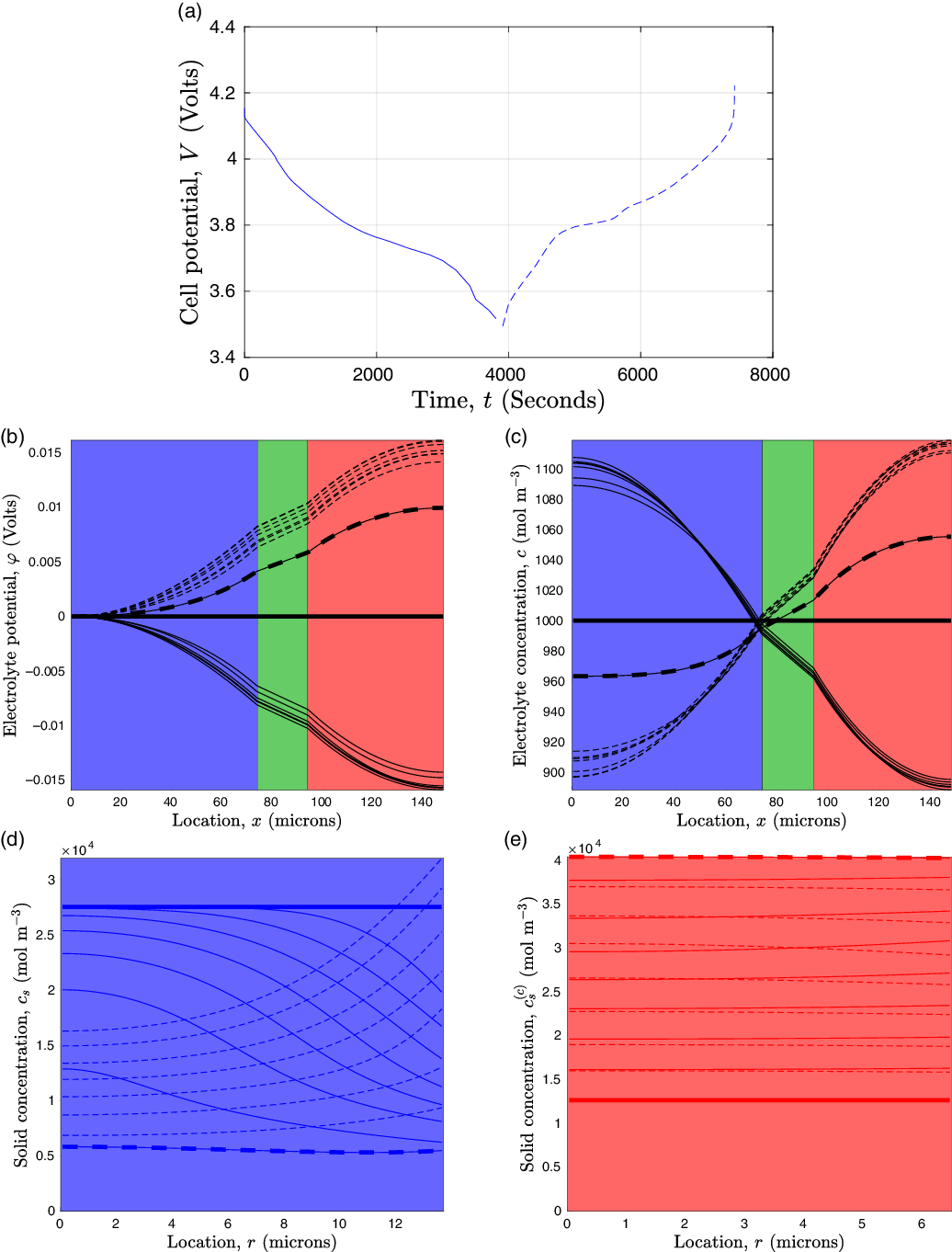
Discharge (solid curves) and subsequent recharge (dashed curves) of a graphite-LNC cell bathed in 1M LiPF
 $_6$
electrolyte at a relatively high rate of 1.3 A. The full parameterisation is give in Table 1. Thick curves indiciate profiles at the beginning of the (dis)charge stages and the different snapshots are taken every 50 s. Panels (a)–(c) show the cell potential, electrolyte potential and electrolyte concentrations respectively, and panels (d) and (e) indicate profiles within an anode and cathode particle both of which are located half way through the thickness of their respective electrodes.
$_6$
electrolyte at a relatively high rate of 1.3 A. The full parameterisation is give in Table 1. Thick curves indiciate profiles at the beginning of the (dis)charge stages and the different snapshots are taken every 50 s. Panels (a)–(c) show the cell potential, electrolyte potential and electrolyte concentrations respectively, and panels (d) and (e) indicate profiles within an anode and cathode particle both of which are located half way through the thickness of their respective electrodes.
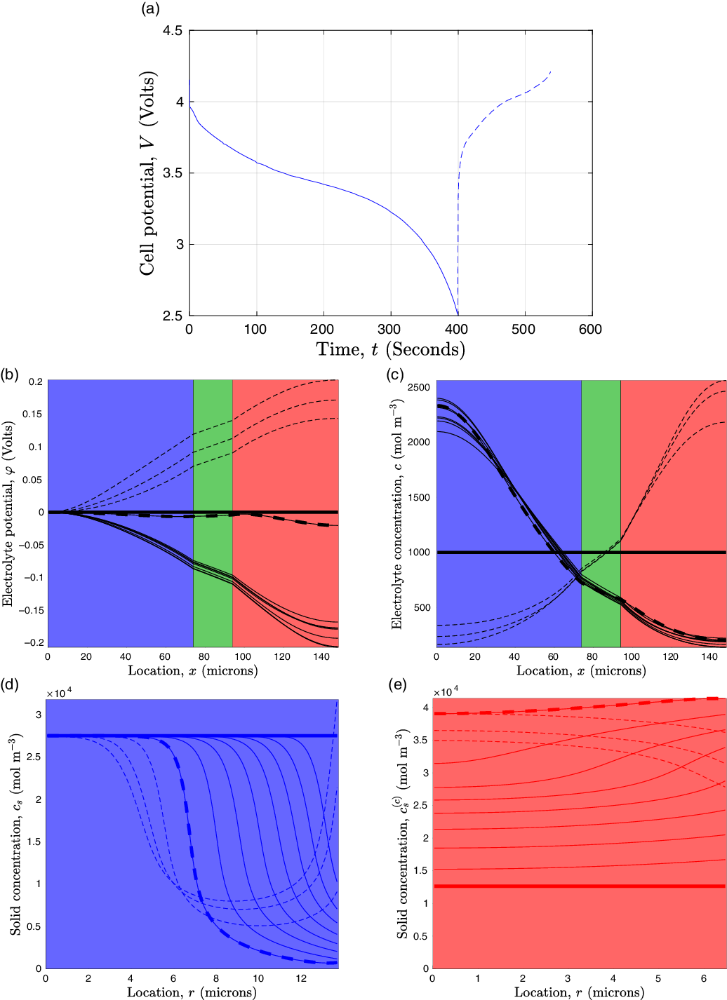
Figure 7 shows the same undergoing a similar discharging and subsequent recharging protocol, but at a more aggresive demand of 1.3 A for a shorter time of 400 s, followed by a subsequent aggresive recharging again at 1.3 A. Note that this faster discharge supplies the same amount of charge to the external circuit as the slower protocol but in a time window 10 times smaller. At the increased rate, we observe that gradients in the electrolyte are much more pronounced, and in fact they are sufficiently large that the deep regions of the cathode approach depletion during discharge. The same is true in the anode during recharging. This larger polarisation contributes to a diminished cell voltage during discharge and we can observe that at the deepest discharge state the voltage has dropped to 2.5 V, which is markedly lower than the 3.5 V attained during the slower protocol despite the devices supplying the same amount of charge. There are now also noticeable concentration gradients within the LNC electrode particles and gradients in the graphite particles are very high. Once again, it is the graphite which ultimately causes recharging to terminate because the surface of the graphite particles becomes saturated and the recharging can only for around 140 s.
5.1 Numerical solutions to the pseudo-2d model
The solutions shown in Figures 6 and 7 were determined numerically using an ultra-fast and robust solver called DandeLiion, the details of which are described in [Reference Korotkin, Sahu, O'Kane, Richardson and Foster54] and available to use at https://www.dandeliion.com. Whilst is is beyond the scope of this work to reiterate, in detail, the workings of the numerical methods used it is pertinent to outline the approach and highlight some of difficulties in solving (4.15)–(4.22c) numerically.
First, a spatial mesh is defined. We introduce
 $N^{(a)}$
grid points across the anode for
$N^{(a)}$
grid points across the anode for
 $x \in (L_1,L_2)$
,
$x \in (L_1,L_2)$
,
 $N^{(s)}$
across the separator for
$N^{(s)}$
across the separator for
 $x \in (L_2,L_3)$
and
$x \in (L_2,L_3)$
and
 $N^{(c)}$
across the cathode for
$N^{(c)}$
across the cathode for
 $x \in (L_3,L_4)$
. At each point in the anode and cathode, a microscopic transport problem must be solved and so at each of the
$x \in (L_3,L_4)$
. At each point in the anode and cathode, a microscopic transport problem must be solved and so at each of the
 $N^{(a)}+N^{(c)}$
grid points a further M grid points need to be introduced to on which to discretise the microscopic transport equations within the electrode particles. Consequently, the complete discrete geometry is comprised of
$N^{(a)}+N^{(c)}$
grid points a further M grid points need to be introduced to on which to discretise the microscopic transport equations within the electrode particles. Consequently, the complete discrete geometry is comprised of
 $(N^{(a)}+N^{(c)}) \times M + N^{(a)} + N^{(s)} + N^{(c)}$
grid points. Second, a suitable approximation (e.g. finite volumes or finite elements) can be used to remove the spatial derivatives and reduce the problem to a large system of coupled differential-algebraic equations (DAEs). The algebraic equations arise largely from the elliptic PDEs, for example, those for the electron conduction in the solid (4.18), whereas the ordinary differential equations arise from the parabolic PDEs, for example, those for transport in the electrode particles (4.20a)–(4.20c). We note the importance of using a spatial discretisation method which is conservative; if such a method is not used, on repeated cell cycling, the total amount of lithium within the system changes markedly and introduces significant errors. It is for this reason that many approaches based on finite difference approximations are not recommended. Third, a scheme for time stepping the system of DAEs must be found. The DandeLiion software uses a selection of implicit backward differentiation formula methods, of orders 1–6, and also offers adaptive time stepping. The choices of time stepping methods is restricted, in comparison to those that can be used for pure ordinary differential equation (ODE) systems, because of the additional constraints imposed by the algebraic equations.
$(N^{(a)}+N^{(c)}) \times M + N^{(a)} + N^{(s)} + N^{(c)}$
grid points. Second, a suitable approximation (e.g. finite volumes or finite elements) can be used to remove the spatial derivatives and reduce the problem to a large system of coupled differential-algebraic equations (DAEs). The algebraic equations arise largely from the elliptic PDEs, for example, those for the electron conduction in the solid (4.18), whereas the ordinary differential equations arise from the parabolic PDEs, for example, those for transport in the electrode particles (4.20a)–(4.20c). We note the importance of using a spatial discretisation method which is conservative; if such a method is not used, on repeated cell cycling, the total amount of lithium within the system changes markedly and introduces significant errors. It is for this reason that many approaches based on finite difference approximations are not recommended. Third, a scheme for time stepping the system of DAEs must be found. The DandeLiion software uses a selection of implicit backward differentiation formula methods, of orders 1–6, and also offers adaptive time stepping. The choices of time stepping methods is restricted, in comparison to those that can be used for pure ordinary differential equation (ODE) systems, because of the additional constraints imposed by the algebraic equations.
Implementing the steps outlined above and implementing it in C++ gives rise to a numerical scheme for solving the pseudo-2d model in a very short time on a standard desktop computer. For reference, the simulation results shown in Figures 6 and 7 each took around 5 s to run and were performed on a discretised geometry comprised of 20,300 grid points with 100 spatial points inside the anode, separator, cathode and each of the electrode particles.
6 Conclusion
We have reviewed the existing modelling of charge transport models of LIBs at the cell scale. This includes a description of ionic motion in the electrolyte in both the dilute and the more practically relevant moderately concentrated regimes. We resolve a common source of confusion in electrolyte modelling in the literature which arises from the definition of the electric potential. In the electrochemical literature, this is usually chosen to be the potential measured with respect to a metallic lithium electrode, in contrast the standard definition used in the physics community where it is with respect to a vacuum at infinity. Crucially, this choice of potential affects the coefficients in the electrolyte transport equations. We have also examined the Butler–Volmer relation describing the reaction at the interface between the electrolyte and the solid electrode particles and demonstrated that these should have a particular functional form in order to avoid nonphysical predictions. The dependency in the Butler–Volmer relation should not only account for the solid electrode particle becoming completely intercalated or deintercalated but allow for cases where the electrolyte concentration gets very low. The specific behaviours of various common solid materials used in electrodes have been considered including the dominant mechanisms for lithium transport and the possible modelling approaches that can be used. The problem of upscaling the models from the microscopic (a single-electrode particle) to the macroscale (the whole cell) has been considered and the appropriate approximations discussed that allow the models to account for moderately concentrated electrolyte behaviour reviewed. In addition, numerical solution to the Newman model has been discussed and some representative realistic solutions to the resulting pseudo-2d model have been presented and discussed. It is noteworthy that this model provides a remarkably accurate description of battery performance if accurately parametrised, see [Reference Ecker, Käbitz, Laresgoiti and Sauer29, Reference Ecker, Tran, Dechent, Käbitz, Warnecke and Sauer30] for further details. It is our hope that this work will prove a useful guide to people who are new to this topic allowing them to develop an appreciation of this highly fertile and technologically important area of research.
Acknowledgements
GWR, JMF and CPP are supported by the Faraday Institution Multi-Scale Modelling (MSM) project Grant number EP/S003053/1. AMR gives thanks for the financial support of the Spanish Government under project PID2019-106337GB-I00 for this work. The authors declare that there is no conflict of interest.
Appendix A. An appropriate form of the Gibb’s–Duhem Relation
Consider a homogeneous mixture containing K different species with mole fractions
 $\chi_1, \chi_2, \cdots, \chi_K$
. The chemical potentials of this mixture
$\chi_1, \chi_2, \cdots, \chi_K$
. The chemical potentials of this mixture
 ${\mu}_1, {\mu}_2, \cdots, {\mu}_K$
are defined, in terms of the Gibbs free energy G, by the relations:
${\mu}_1, {\mu}_2, \cdots, {\mu}_K$
are defined, in terms of the Gibbs free energy G, by the relations:
 \begin{eqnarray}{\mu}_i= \frac{\partial G}{\partial n_i} \qquad \mbox{for} \quad i=1,2, \cdots,K, \end{eqnarray}
where
 $n_i$
is the number of moles of species i in the mixture. The Gibb’s free energy of the system is typically written as a function of the number of moles of each species in the mixture, that is,
$n_i$
is the number of moles of species i in the mixture. The Gibb’s free energy of the system is typically written as a function of the number of moles of each species in the mixture, that is,
 $G=G(n_1,n_2, \cdots, n_K)$
. However, since this quantity is extensive and therefore scales linearly with the total number of moles of the mixture
$G=G(n_1,n_2, \cdots, n_K)$
. However, since this quantity is extensive and therefore scales linearly with the total number of moles of the mixture
 $N_{tot}$
, when the mole fractions of the various species are held constant, it can be written in the from
$N_{tot}$
, when the mole fractions of the various species are held constant, it can be written in the from
 \begin{eqnarray}G(N_{tot},\chi_1, \chi_2, \cdots, \chi_K)=N_{tot} h(\chi_1, \chi_2, \cdots, \chi_K), \end{eqnarray}
where here
 $h(\cdot)$
is the Gibbs free energy of the mixture per mole, and
$h(\cdot)$
is the Gibbs free energy of the mixture per mole, and
 $N_{tot}$
and the various mole fractions are defined by:
$N_{tot}$
and the various mole fractions are defined by:
 \begin{eqnarray}N_{tot}=\sum_{k=1}^K n_k \qquad \chi_i=\frac{n_i}{\sum_{k=1}^K n_k}.\end{eqnarray}
Since we are primarily interested in solutions it is more useful to deal with the
 $\tilde{G}$
, the Gibbs free energy of the mixture per unit volume which we can express in the form:
$\tilde{G}$
, the Gibbs free energy of the mixture per unit volume which we can express in the form:
 \begin{eqnarray}\tilde{G}= c_T h(\chi_1, \chi_2, \cdots, \chi_K) \quad \mbox{where} \quad c_T=\sum_{k=1}^K c_k \quad \mbox{and} \quad \chi_i=\frac{c_i}{\sum_{k=1}^K c_k}, \end{eqnarray}
in which
 $c_k$
(for
$c_k$
(for
 $k=1,\cdots K$
) are the molar concentrations of the various species and
$k=1,\cdots K$
) are the molar concentrations of the various species and
 $c_T$
is the total molar concentration of the mixture.Footnote
7
In this case, where we express, the volumetric Gibb’s free energy in the form
$c_T$
is the total molar concentration of the mixture.Footnote
7
In this case, where we express, the volumetric Gibb’s free energy in the form
 $\tilde{G}=\tilde{G}(c_1,c_2, \cdots,c_K)$
it is clear that the chemical potentials (see (A1)) can be expressed in the form:
$\tilde{G}=\tilde{G}(c_1,c_2, \cdots,c_K)$
it is clear that the chemical potentials (see (A1)) can be expressed in the form:
A summary of the most important nomenclature
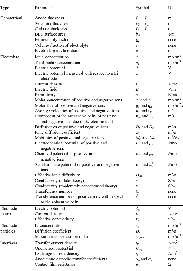
 \begin{eqnarray}{\mu}_q= \frac{\partial \tilde{G}}{\partial c_q} \qquad \mbox{for} \quad q=1,2, \cdots,K, \end{eqnarray}
The Gibbs–Duhem relations.
The form of the Gibbs–Duhem relation that we shall require is
 \begin{eqnarray}\sum_{q=1}^K c_q \frac{\partial {\mu}_q}{\partial c_i}=0, \quad \mbox{for} \quad i=1,2, \cdots K. \end{eqnarray}
In order to show that these relations are true, we start by defining the quantities:
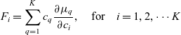 \begin{eqnarray}F_i=\sum_{q=1}^K c_q \frac{\partial {\mu}_q}{\partial c_i}, \quad \mbox{for} \quad i=1,2, \cdots K\end{eqnarray}
which are equivalent to the left-hand side of (A6). We can re-express the
 $F_i$
, by using the expressions for the chemical potentials (A5), as follows:
$F_i$
, by using the expressions for the chemical potentials (A5), as follows:
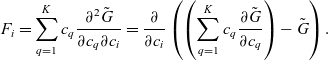 \begin{eqnarray}F_i=\sum_{q=1}^K c_q \frac{\partial^2 \tilde{G}}{\partial c_q \partial c_i}= \frac{\partial}{\partial c_i} \left( \left( \sum_{q=1}^K c_q \frac{\partial \tilde{G}}{\partial c_q} \right) -\tilde{G} \right). \end{eqnarray}
We can now use the expression for the Gibb’s free energy density, contained in (A4), and the chain rule to re-express the partial derivative
 $\partial \tilde{G}/\partial c_q$
in terms of the mole fractions
$\partial \tilde{G}/\partial c_q$
in terms of the mole fractions
 $\chi_k$
and the function h:
$\chi_k$
and the function h:
 \begin{eqnarray*}\frac{\partial \tilde{G}}{\partial c_q}=h+\frac{\partial h}{\partial \chi_q} - \sum_{j=1}^K \chi_j \frac{\partial h}{\partial \chi_j}.\end{eqnarray*}
From this, it becomes apparent that
 \begin{eqnarray*}\sum_{q=1}^K c_q \frac{\partial \tilde{G}}{\partial c_q}=c_T \left[ \sum_{q=1}^K \left(\chi_q h+ \chi_q \frac{\partial h}{\partial \chi_q} - \chi_q \sum_{j=1}^K \chi_j \frac{\partial h}{\partial \chi_j} \right)\right].\end{eqnarray*}
Making use of the fact that
 $\sum_{q=1}^K \chi_q=1$
and that
$\sum_{q=1}^K \chi_q=1$
and that
 $\tilde{G}=c_T h$
the above expression can be simplified to
$\tilde{G}=c_T h$
the above expression can be simplified to
 \begin{eqnarray}\sum_{q=1}^K c_q \frac{\partial \tilde{G}}{\partial c_q}=\tilde{G}. \end{eqnarray}
Substituting (A9) into (A8) immediately gives the desired results, namely that
 $F_i=0$
for
$F_i=0$
for
 $i=1,2, \cdots K$
and thus proves the Gibbs–Duhem relations (A6).
$i=1,2, \cdots K$
and thus proves the Gibbs–Duhem relations (A6).

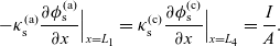


 Open access