2.1. Dimensional model

Let us consider a 2-D hillslope of length $L_x$ with a uniform terrain slope $S_x$, uniform thickness of the porous layer $L_z$, uniform saturated soil hydraulic conductivity $K_s$ and an impenetrable bedrock beneath the hillslope. As shown in the $(x,z)$-plane in figure 2, we denote the thickness of the saturated zone as $H_g(x,t)$ and the height of the surface water as $h_s(x,t)$.

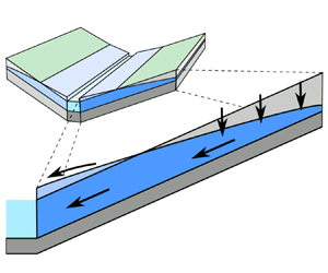
Figure 2. Hillslope geometry used to formulate a 1-D surface–subsurface model.

We shall assume that overland flow can only occur when the soil becomes fully saturated. The overland flow generated by exceeding the soil infiltration capacity (Kirkby Reference Kirkby2019) is not considered. Under this assumption, the heights $H_g$ and $h_s$ can be combined to form a single dependent variable,

(2.1)\begin{equation} H(x,t) = H_g(x,t) + h_s(x,t), \end{equation}

defined as the total height of groundwater and surface water. We now review the governing equations for $H$, for which the details are presented in Appendix B.

2.1.1. Groundwater flow

The standard approach to model shallow-water aquifers uses the Dupuit–Forchheimer assumption, which states that groundwater flows horizontally with the pressure head following a hydrostatic profile. Under this approximation, the groundwater flow is given by

(2.2)\begin{equation} Q_g = K_s H\frac{\partial H}{\partial x} + K_s H S_x. \end{equation}

When the soil is not fully saturated, and hence $H< L_z$, the evolution of the groundwater depth is given by the continuity equation, resulting in a standard form of the Boussinesq equation (Troch et al. Reference Troch2013) for an unconfined aquifer:

(2.3)\begin{equation} f(x, t) \frac{\partial H_g}{\partial t} = \frac{\partial }{\partial x}Q_g + r = \frac{\partial }{\partial x}\left(K_s H_g\frac{\partial H_g}{\partial x} + K_s H_g S_x\right) + r(x,t), \end{equation}

where $r(x,t)$ denotes the groundwater recharge, and $f(x, t)$ is a drainable porosity. In this paper, we assumed that the recharge is equal to the precipitation.

The drainable porosity function is more subtle; as introduced in Appendix C, it is formally defined as the rate of change of groundwater volume, $\mathcal {V}$, given a change in the groundwater level, $H$, i.e. $f={\rm d}\mathcal {V}/{\rm d} H$. Note that $f$ depends on the soil saturation above the groundwater table. For example, higher soil saturation implies that less water is required to raise the groundwater by a given volume and, hence, $f$ is lower. Recall that the soil saturation, $\theta$, is computed as a function of the pressure head, $h_g$, as given by the Mualem–van Genuchten model (C3). In theory, computing $f$ would involve coupling equation (2.3) with a model for $h_g(x, z,t)$.

In the literature (e.g. Troch et al. Reference Troch, Paniconi and Emiel van Loon2003), $f$ is often assumed to be a parameter with a value specific to the soil type at a given location. In practice, however, $f$ can change over time. For example, during a rainfall, a characteristic wetting front forms, which slowly propagates from the surface towards the groundwater table (Caputo & Stepanyants Reference Caputo and Stepanyants2008). In order for this table to rise, the rainwater must first infiltrate through the unsaturated zone. This causes $f$ to significantly change over time.

In this paper, we approximate $f(x, t)$ by a time-independent mean drainable porosity $f_{{mean}}(x)$. Although the model results will not duplicate the full time-dependent behaviour observed in Part 2, the mean value, $f_{{mean}}(x)$, is chosen such that solutions correctly capture the key time when the groundwater reaches the land surface. We show later that the resultant model reproduces the hydrograph during a single precipitation event (see figure 9 later).

In Appendix C, we justify the choice of

(2.4)\begin{equation} f(x, t) \approx f_{{mean}}(x) \equiv \frac{v_H(x)}{D(x)}, \end{equation}

where $v_H(x)$ is the initial drainable volume per unit area at a given location, and $D(x)=L_z-H(x)$ is the depth of the groundwater below the land surface. In other words, the drainable porosity is given by the fraction of the soil volume that can be filled with water. Henceforth, we take the mean approximation (2.4) as the definition of $f$. Further discussion of the drainable porosity function is provided in Appendix C, where we provide formulae for its implementation.

2.1.2. Coupling with the overland flow

Now let us consider the case where the soil is fully saturated, for which $H_g = L_z$, which implies $H>L_z$. In this case, as derived in Appendix B, the surface depth $h_s$ evolves according to the following continuity equation:

(2.5)\begin{equation} \frac{\partial h_s}{\partial t} = \frac{\partial }{\partial x}(Q_g + Q_s) + r = \frac{\partial }{\partial x}\left(K_s L_z \frac{\partial h_s}{\partial x} + \frac{\sqrt{S_x}}{n_s} h_s^k\right) + r(x,t). \end{equation}

In the above equation, we have used Manning's equation to represent the overland flow:

(2.6)\begin{equation} Q_s = \frac{\sqrt{S_f}}{n_s} h_s^k \sim \frac{\sqrt{S_x}}{n_s} h_s^k, \end{equation}

where $k=5/3$ and $n_s$ is the Manning roughness coefficient, which depends on the hillslope surface type and is determined empirically. We use the kinematic approximation ($S_f \sim S_x$), where the friction slope $S_f$ is only dependent on the elevation gradient $S_x$. Alternatively, we could also consider the diffusive approximation $S_f\sim S_x+{\partial h_s}/{\partial x}$; however, we limit this study to the kinematic approximation only for simplicity.

Furthermore, we note that apart from the constant gravitationally-induced groundwater flow, the pressure difference caused by the gradient of surface water height may affect the groundwater flow. Typically, the size of the overland flow is negligibly small compared with the thickness of the porous layer. However, as we discuss in § 5, this approximation fails at the propagating seepage front, which requires us to include the $({\partial }/{\partial x})(K_s L_z ({\partial h_s}/{\partial x}))$ diffusion term.

Now, we can combine (2.3) and (2.5) into a single equation for $H$:

(2.7) \begin{equation} \frac{\partial H}{\partial t} =\begin{cases} \displaystyle f(x)^{{-}1}\left[\frac{\partial }{\partial x}\left(K_s H\frac{\partial H}{\partial x} + K_s H S_x\right) + r\right] & \text{if } H \leq L_z, \\ \displaystyle \frac{\partial }{\partial x}\left[K_s L_z \frac{\partial H}{\partial x} + \frac{\sqrt{S_x}}{n_s} (H-L_z)^k\right] + r & \text{if } H > L_z. \end{cases} \end{equation}

We assume a no-flow boundary condition at the catchment boundary ($x=L_x$). At the location of the river ($x=0$), we assume that the river table is located at the same level as the overland water height (or at the surface if no overland flow is present). Therefore, at $x=0$ we set $H_g=L_z$ and a (flat) free-surface condition for the overland flow, $\partial h_s/\partial x = 0$. In addition, in this work, we study the time evolution of the above system assuming that it is initially in equilibrium for a given mean rainfall $r_0< r$, and then subjected to a rainfall $r$ for $t > 0$. Therefore, for the initial condition, we take the steady-state of equation of (2.7) for a given mean rainfall $r_0$. The boundary and initial conditions are summarised shortly in § 2.3.

2.2. Non-dimensional model

The above model can be non-dimensionalised by taking $x = L_x x'$, $t = T_0 t'$, $H=L_z H'$ and $r=r_0r'$. Here, $T_0= L_x/(K_sS_x)$ is a characteristic timescale of the groundwater flow, chosen to balance the temporal term and the $\partial _x(K_s H S_x)$ term.

Once non-dimensionalised, our governing equations (2.7) become (after dropping primes)

(2.8a) \begin{equation} \frac{\partial H}{\partial t} =\begin{cases} \displaystyle f(x)^{{-}1}\left[\frac{\partial }{\partial x}\left(\sigma H\frac{\partial H}{\partial x} + H\right) + \rho_0 r(x, t)\right] & \text{if } H \leq 1, \\ \displaystyle \frac{\partial }{\partial x}\left(\sigma\frac{\partial H}{\partial x} + \mu (H-1)^k\right) + \rho_0 r(x,t) & \text{if } H > 1, \end{cases} \end{equation}

and the dimensionless parameters $\sigma$, $\mu$ and $\rho _0$ are introduced shortly in § 2.3. In this work, we assume that the rainfall is constant and uniform, i.e. $r(x, t) = r = \text {constant}$, except for the initial jump from $r_0$ to $r>r_0$. However, we shall discuss in § 10 that our methodology can be applied in the case of time-dependent rainfall.

In combination with the governing equations (2.8a), we have to specify the dimensionless boundary conditions. First, at $x = 0$, we need to consider two situations. First, if a seepage zone exists for the initial $r_0$, we set a free flow boundary condition,

(2.8b)\begin{equation} H_x(0, t) = 0. \end{equation}

However, as we shall demonstrate in § 3.1, if $r_0$ is low enough, initially the seepage does not exist. Then we assume that $H(x,t)$ representing groundwater is reaching the surface at $x=0$, i.e.:

(2.8c)\begin{equation} H(0, t) = 1. \end{equation}

During a rainfall ($r>r_0$), the groundwater gradient at $x=0$, which is initially negative, increases as the groundwater rises. The seepage starts to grow, when the when it becomes positive, which is when boundary condition (2.8c) is replaced with (2.8b).

At the right-hand edge, by the definition of a catchment, there is zero flow:

(2.8d)\begin{equation} Q(1, t) = 0, \end{equation}

where the dimensionless total flow, $Q$, is defined as

(2.9) \begin{equation} Q(x, t) =\begin{cases} \displaystyle H + \sigma H\frac{\partial H}{\partial x} & \text{if } H \leq 1, \\ \displaystyle 1 + \sigma\frac{\partial H}{\partial x} + \mu(H-1)^k & \text{if } H > 1. \end{cases} \end{equation}

For the initial condition, $H(x,t=0)=H_0(x)$, we take a steady state of (2.8a) for $r=1$:

(2.10) \begin{equation} 0 =\begin{cases} \displaystyle\frac{\partial }{\partial x}\left(\sigma H_0\frac{\partial H_0}{\partial x} + H_0\right) + \rho_0 & \text{if } H_0 \leq 1, \\ \displaystyle\frac{\partial }{\partial x}\left(\sigma\frac{\partial H_0}{\partial x} + \mu \left(H_0-1\right)^k\right) + \rho_0 & \text{if } H_0 > 1. \end{cases} \end{equation}

In this paper, we refer to this model (2.8) as the 1-D model.

2.3. The non-dimensional parameters

In the first case of (2.8), we have introduced two key dimensionless parameters, defined as

(2.11a)\begin{gather} \sigma =\frac{L_z}{L_xS_x} = \frac{\textrm{thickness of the porous layer}}{\textrm{elevation drop along the hillslope}}, \end{gather}

(2.11b)\begin{gather}\rho_0 =\frac{r_0 L_x}{L_z S_x K_s} = \frac{\textrm{precipitation flux}}{\textrm{maximum groundwater flux}}. \end{gather}

Note that $\sigma \to \infty$ as the hillslope becomes increasingly flat. The parameter $\rho _0$ represents the ratio of the total precipitation rate (given by $rL_x$ in $\mathrm {m}^2\ \mathrm {s}^{-1}$) to the maximum possible groundwater flow for fully saturated soil (given by $L_z S_x K_s$ in $\mathrm {m}^2~\mathrm {s}^{-1}$). Introduction of the maximum groundwater discharge is a classic concept in hydrology, see, e.g. Horton (Reference Horton1936).

In the second case of (2.8), we have introduced an additional dimensionless parameter:

(2.12)\begin{equation} \mu = \frac{L_z^{k-1}}{K_sS_x^{1/2}n_s}. \end{equation}

We argue later in § 6.2 that the characteristic size of the overland flow scales as $L_s=\mu ^{-1/k}L_z$. Following that section, we introduce a key dimensionless parameter to describe the dynamics in the seepage zone, namely the Péclet number:

(2.13)\begin{equation} Pe =\frac{\mu^{1/k}}{\sigma}=\frac{\dfrac{\sqrt{S_x}}{n_s}L_s^{k}}{K_sL_z\dfrac{L_s}{L_x}} =\frac{\text{convective overland flow}}{\text{diffusive effect of the groundwater flow}}. \end{equation}

In order to interpret ${Pe}$, we note that the numerator represents the second term on the right-hand side of (2.7) for $H>L_z$, representing convective effects. The denominator represents the size of the first term on the right-hand side of (2.7) for $H>L_z$, representing diffusive effects.

Based on median values of physical parameters used in the above equations provided in table 1, we have $\sigma \approx 10^{-2}$, $\rho _0\approx 1.5$, $\mu \approx 10^7$ and ${Pe}\approx 10^5$. Consequently, our work primarily focuses on the limits of $\mu, \, {Pe} \to \infty$, where convection dominates diffusion.

Table 1. Typical values of physical parameters characterising UK catchments extracted in Part 1 of this paper (Morawiecki & Trinh Reference Morawiecki and Trinh2024a).

3.1. Typical results for $\rho _0 < 1$ and $\rho _0 > 1$

The existence of the seepage zone in the initial steady state depends on whether the value of $\rho _0$, defined in (2.11b), is higher or lower than $1$, and each case exhibits a different transient behaviour. Typical solutions obtained in these two cases are shown in figure 3.

Figure 3. Schematic presenting early- and late-time dynamics for a catchment with and without an initial seepage zone (corresponding to $\rho _0>1$ and $\rho _0\leq 1$ respectively). In (a), (b) and (c) a seepage zone is observed, and therefore a separate graph is presented to illustrate the evolution of the surface water depth (note that the vertical axis is multiplied by the scaling factor $\mu ^{1/k}\approx 3260$).

First, consider figure 3(a,b). In the case of $\rho _0>1$, we already have a seepage zone in the initial state. In a short timescale, the height of the surface water increases quickly until reaching a seemingly quasi-static state. Afterwards, the flow continues to increase as a result of the saturation front propagating uphill, but this process is characterised by a much longer timescale and a slower rate of flow rise. The difference between the short- and long-time behaviour can also be seen in the produced hydrograph in figure 4. It shows the dependence between the total river inflow, defined as the total flow (2.9) evaluated at the river bank ($x=0$),

(3.3)\begin{equation} Q(t)=Q(x=0,t). \end{equation}

In the presented hydrograph, we have marked the initial fast transition as (A) and the subsequent slow transition as (B).

Figure 4. Schematic representation of the hydrograph obtained for a catchment with and without an initial seepage zone (corresponding to $\rho _0>1$ and $\rho _0\leq 1$, respectively). Points represent times for which the profiles are shown in figure 3, whereas letters A–D refer to corresponding phases from that figure.

For $\rho _0<1$, we do not observe an initial seepage zone, i.e. $H(x,t=0)<1$ for all $x$. For some time the groundwater table is rising, increasing groundwater flow reaching the river, until the groundwater depth gradient at $x=0$ becomes $0$. Then the seepage zone starts to slowly form and propagate away from the channel, increasing the overland flow reaching the river.

However, in practice, in the case of real-world catchments characterised by a thin porous layer (which is a base assumption behind the presented 1-D model), the groundwater flow rate is highly limited. Therefore, in such catchments, we expect the $\rho _0>1$ case to be more prevalent, which is additionally confirmed by low base flow index (BFI) values characterising low-productive catchments. (BFI describes the ratio between the base flow and total flow in the given catchment. High values refer to catchments dominated by the groundwater flow, whereas low values refer to catchments with a significant overland flow component.) Therefore, in this paper, we focus on discussing the mathematical properties of each phase presented in figure 4 only in the case of $\rho _0>1$.

In general, the solution for the PDE model (2.8a) can only be found numerically. However, by taking advantage of the typical sizes of dimensionless parameters, the model can be further simplified. Figure 5 shows the effect of dimensionless parameters, $\rho$, $\rho _0$, $\sigma$ and $\mu$ on the model's solution. The graphs in the left column show how the initial steady state $H_0(x)$ depends on the value of each parameter, whereas the graphs on the right present the effect of each parameter on the hydrograph $Q(x=0,t)$. The conclusions from this numerical experiment are as follows.

1. (i) Parameter $\rho _0$ (typical value $2$), which following (2.11b) characterises the mean precipitation rate in terms of the groundwater flow, has a significant effect on the initial steady state. As discussed in detail previously, $\rho _0<1$ corresponds to a hillslope with no initial seepage zone, and is characterised by different dynamics than the $\rho _0>1$ case, in which we observe a fast rise of flow in the early time. In most of this paper, we consider only the latter case.

2. (ii) Parameter $\rho$ (typical value $\approx$20), which characterises the simulated precipitation rate in terms of the groundwater flow, does not affect the initial steady state, but it does affect how quickly the flow is rising. Higher $\rho$ values lead to both a higher flow over the seepage zone and a faster growth of this zone. Values of $\rho$ can vary significantly depending on the rainfall event considered.

3. (iii) Parameter $\sigma$ (typical value $10^{-2}$), which following (2.11a) characterises the thickness of porous layer compared with the elevation drop along the hillslope, has a significant effect only on the solution outside the seepage zone. In the case of the seepage zone, the term including $\sigma$ is negligibly small compared with the $\mu$ term. However, it affects the speed at which the seepage zone is growing. Note that as $\sigma \rightarrow 0$, the initial groundwater shape becomes a linear function (with a possible small boundary layer at its left border). Even though this limit is not critical in our analysis, it may allow us to approximate the initial groundwater shape without the need to solve the governing equations numerically.

4. (iv) Parameter $\mu$ (typical value $10^6$), which following (2.12) characterises the overland flux, does not have a significant effect on the groundwater table outside the seepage zone, but it has a major effect on the height of the surface water within the seepage zone. Higher $\mu$ values correspond to lower surface water height, which in the limit $\mu \rightarrow \infty$ becomes negligible compared with the variation of the groundwater depth. In addition, in this limit, the seepage zone size reaches a limiting value, $a_0=1-{1}/{\rho _0}$ (see § 5). This limit is strongly supported by real-world data (typical value of $\mu$ for UK catchments is of the order of $10^6$ based on the typical parameter values estimated in Part 1 of this study), and it allows us to derive the formula for a typical hydrograph.

Figure 5. Effect of dimensionless parameters shown for the initial steady state $H_0(x)$ versus $x$ (insets left column) and for the hydrograph $Q(t)$ versus $t$ (insets right column). Inset (a) shows changing $\rho _0$; inset (b) shows changing $\rho$; inset (c) shows changing $\sigma$; and inset (d) shows changing $\mu$. In the case of (a), (c) and (d), solid lines represent solutions for $\rho _0=1.5$ (scenario with an initial seepage zone), and dashed lines represent solutions for $\rho _0=0.6$ (scenario without an initial seepage zone). The surface water ($H>0$) is magnified 1000 times.

5.1. Analytical solution as $\sigma \to 0$

One quite useful limit is to consider $\sigma \rightarrow 0$, corresponding to the infinitely thin porous layer limit. In Appendix E, we derive the outer asymptotic expansion for $H_0$ in terms of $\sigma$, (E2), its inner expansion around $x=0$ (E4), and finally match them to form the following composite approximation for $H_0(x)$:

(5.7)\begin{equation} H_0(x)=\rho_0(1-x+\sigma-\sigma \,{\rm e}^{-{(x-a_0)}/{\sigma}}), \quad \text{for } x \in [a_0, 1]. \end{equation}

As shown in figure 6, this asymptotic solution provides a good approximation of the groundwater shape both for small $\sigma$ values and, surprisingly, also for large $\sigma$ values. In the latter case, $H_0$ becomes a quadratic function,

(5.8)\begin{equation} 1-H_0\sim \frac{\rho_0}{2\sigma}(x-a_0)^2, \end{equation}

which is also a limiting behaviour of our matched asymptotic solution (5.7) as $x\to a_0$.

Figure 6. Comparison of groundwater depth given by (5.6) (full numerical solution) with the matched asymptotic approximation given by (5.7).

6.1. Groundwater rise and propagation of the seepage zone

Having derived certain analytical properties of the steady-state configuration, $H_0(x; \, \rho _0)$ (used as an initial condition), we can now study the short-time behaviour of the system as the rain input is set to $\rho$. As argued at the start of § 4, this is a good approximation, when the rainfall duration is much shorter than the characteristic time of the groundwater transfer to the channel.

As shown in Appendix F, the outer solution outside the seepage zone (4.3b) can be expanded into a regular series expansion in powers of time $t$:

(6.1)\begin{equation} H_{outer}(x,t) \sim H_0(x; \, \rho_0) + \left[\frac{\rho - \rho_0}{f(x)}\right] t + {O}(t^2). \end{equation}

This approximation assumes that $x - a(t) = {O}(1)$. The approximation (6.1) thus indicates that the groundwater rises in a fashion proportional to time and the difference between current and prior rain input; it correctly describes the shape of the groundwater except for a thin boundary layer at $x=a(t)$ of thickness of ${O}(\sqrt {t/(\rho - \rho _0)})$ (see figure 7a). Therefore, for intense rainfall, $\rho \gg 1$, we can neglect the effect of this boundary layer.

Figure 7. (a) Comparison of the numerical solution of the groundwater shape (solid lines) with the outer solution developed in Appendix F (dashed lines) at different times $t$. The corresponding size of the seepage zone is presented in (b). A small region is magnified to highlight differences between the presented approximations. The lines are not smooth due to the $h(x)$ interpolation error.

We may use the outer groundwater approximation, (6.1), in order to predict the motion of the contact line, $x = a(t)$. Setting $H_{outer} = 1$ gives, in implicit form,

(6.2)\begin{equation} t \sim \frac{f(x=a(t))}{\rho - \rho_0} (1 - H_0(x=a(t))) \equiv \mathcal{T}(x=a(t)). \end{equation}

In order to calculate the above, we must solve two first-order ODEs: (5.6) for the height, $H_0(x)$, and (C2) for the head, $h_g(\hat {z})$, itself used in the calculation of $f(x)$. Alternatively, one can use the analytical approximations for $H_0(x)$ given by (5.7), and $f(x)$ given by (C6) or (C7). Figure 7(b) compares these approximations with the location of the saturation front computed from a full numerical solution of the 1-D model. As we observe based on the difference between the full numerical solution and leading-order approximation (LOA), neglecting the boundary layer around $a(t)$ introduces a small error when estimating the seepage zone size. Replacing the ODEs with analytical approximations for $f(x)$ and $H_0(x)$ in (6.2) also introduces an error, but it is significantly smaller.

6.2. Evolution of the overland flow

Now, knowing how the seepage zone propagates, we can develop a time-dependent solution for the overland flow. Our goal is to extract how the overland flow into the river, $Q_s(x=0, t)$, evolves in time, taking into account the effects of increased rainfall and the seepage zone growth.

6.2.1. Problem reduction under ${Pe}\rightarrow \infty$ limit

The equation for overland flow is given by (4.3a) with the initial condition satisfying steady state (5.1b). We rescale according to

(6.3)\begin{equation} \eta = \mu^{1/k}(H-1) \quad \text{and} \quad T = \mu^{1/k}t. \end{equation}

Here, $\eta = \eta (x, T)$ is the rescaled surface water height $h_s=H-1$. Then (4.3a) can be written as

(6.4)\begin{equation} \frac{\partial \eta}{\partial T} - k \eta^{k-1}\frac{\partial \eta}{\partial x} - {Pe}^{{-}1}\frac{\partial^2 \eta}{\partial x^2}= \rho, \end{equation}

and (5.1b), which provides the initial condition, $H_0$, is

(6.5)\begin{equation} 1 + \eta^k - {Pe}^{{-}1} \dfrac{{\rm d}\eta}{{\rm d}\kern 0.06em x} = \rho_0 (1 - x), \end{equation}

where, as before, ${Pe}^{-1}=\sigma /\mu ^{1/k}$. Following (4.3a) and (4.3c) the boundaries conditions are

(6.6a,b)\begin{equation} \partial_x \eta(0, t) = 0, \quad \eta(a(t), t) = 0. \end{equation}

Note that the characteristic time it takes the overland flow to reach the channel ($\mu ^{-1/k}T_0\approx 0.1\ \textrm {day}$) is much shorter than the characteristic time describing the groundwater flow ($T_0\approx 1000\ \textrm {days}$), and has a similar order of magnitude as a typical rainfall duration. As a result, a short-time approximation is not satisfactory to describe flow variation during a single rainfall event.

The solution for general times can be obtained by considering the ${Pe} \rightarrow \infty$ limit, similarly as we did when analysing the steady state. This limit allows us to neglect the diffusion term everywhere except for a negligibly thin boundary layer around $x=a$.

In the limit ${Pe} \rightarrow \infty$, we expand $\eta = \eta _0 + {Pe}^{-1} \eta _1 + \cdots$, and (6.4) becomes a first-order hyperbolic PDE:

(6.7a)\begin{equation} \frac{\partial \eta_0}{\partial T} - [k \eta_0^{k-1}]\frac{\partial \eta_0}{\partial x}= \rho, \quad x \geq 0. \end{equation}

For $0 \leq x \leq a(t)$, there is an initial condition given by

(6.7b)\begin{equation} \eta_0(x, 0) = \rho_0^{1/k}(a_0-x)^{1/k}, \end{equation}

where we have used the fact shown in Appendix D that $a_0=1-1/\rho _0$ (cf. (5.5)). The above initial condition is defined along the entire initial seepage zone, $x\in [0,a_0]$. Note that neglecting the diffusion term results in a kinematic wave equation, for which the downstream boundary condition (6.6a) is no longer required.

6.2.2. Implicit solution using methods of characteristics

The system (6.7) can be solved using the method of characteristics (Lagrange–Charpit equations). The solution is given by characteristic curves $(T, x, \eta _0)$, now parameterised by $(s, \tau )$, where $\tau$ is the characteristic curve parameter, and $s$ parameterises the initial data. The characteristic equations are

(6.8a) \begin{equation} \dfrac{{\rm d}T}{{\rm d}\tau}=1, \quad \dfrac{{\rm d}\kern 0.06em x}{{\rm d}\tau}={-}k\eta_0^{k-1}, \quad \dfrac{{\rm d}\eta_0}{{\rm d}\tau}=\rho. \end{equation}

The initial conditions are specified along $\tau = 0$ according to two types of characteristics. One set of characteristics emerges from $T = 0$, at the location of the initial water shape, $H_0(x)$, valid for $x\in [0, a(t)]$. Another set of characteristics emerges from the propagating front, $x = a(t)$, representing the groundwater reaching the surface and, hence, initiating surface flow.

Parameterising the initial data by $x = s$, we have

(6.8b) \begin{equation} (T(s, 0), x(s, 0), \eta_0(s, 0)) =\begin{cases} (0, s, H_0(s)), & s \in [0, a(t)], \\ (\mu^{1/k}\mathcal{T}(s), s, 0), & s \in [a(t), \infty). \end{cases} \end{equation}

The first condition will use the initial surface height, $H_0(s) = \rho _0^{1/k}(a_0-s)^{1/k}$ given by (6.7b). The second condition is essentially specified along the moving front, $(T, x, \eta _0) = (T, a(t), 1)$, but we have written it in terms of the $s$-independent variable, and the rescaled function $\mathcal {T}$ in (6.2). In summary, the characteristic solution can be obtained via direct integration of (6.8), giving

(6.9) \begin{equation} \left.\begin{array}{c@{}} T(s,\tau)=T(s,0)+\tau, \\ x(s,\tau)=x(s,0)-\rho^{{-}1}[\eta_0(s,0)+\rho\tau]^k+\rho^{{-}1}[\eta_0(s,0)]^k, \\ \eta_0(s,\tau)=\eta_0(s,0)+\rho\tau. \end{array}\right\} \end{equation}

We show an example of the characteristics and characteristic projections in figure 8.

Figure 8. Characteristic curves given by (6.9) for parameters listed in table 1. Dark blue lines represent curves originating from the initial seepage zone, and light green lines represent curves originating from the propagating front of the seepage zone.

Once the solution is determined, a key quantity of interest is the surface water height at $x = 0$, as it determines the overland flow reaching the river. We denote this critical point along the characteristics as $(T, \eta _0) = (T^*, \eta ^*)$. By setting $x(s,\tau )=0$ in the characteristic equations (6.9) and eliminating $\tau$ from the second equation, we obtain

(6.10)\begin{equation} \begin{pmatrix} T^* \\ \eta^* \end{pmatrix}=\begin{pmatrix} T(s,0)+\dfrac{1}{\rho}(\eta^*-\eta_0(s,0)) \\ (\rho x(s,0)+(\eta_0(s,0))^k)^{1/k} \end{pmatrix}. \end{equation}

We need to consider two cases separately: characteristics starting from the initial seepage zone and characteristics emerging from the propagating seepage front. Each case is given by the different initial conditions, as specified in (6.8b).

In the first case, by substituting the first initial condition from (6.8b) into (6.10), we obtain

(6.11)\begin{equation} \begin{pmatrix} T^* \\ \eta^* \end{pmatrix}=\begin{pmatrix} \dfrac{1}{\rho}(\eta^*-\rho_0^{1/k}(a-s)^{1/k}) \\ (\rho s+\rho_0(a-s))^{1/k} \end{pmatrix}. \end{equation}

By finding $s$ from (6.12a) and substituting into (6.12b) we can express $T^*$ as a function of $\eta ^*$:

(6.12)\begin{equation} T^*(\eta^*)=\frac{1}{\rho}\left[\eta^*-\left(\frac{\rho_0}{\rho-\rho_0}\right)^{1/k}(\rho a_0 - (\eta^*)^k)^{1/k}\right]. \end{equation}

This equation is satisfied for $\eta ^*\in [(\rho _0 a_0)^{1/k}, (\rho a_0)^{1/k}]$. The lower limit corresponds to the initial height, and the upper limit corresponds to the height reached by the characteristic curve starting at $x_0=a_0$. At the upper limit, the characteristic curve reaches the river ($x=0$) at what we refer to as the critical time:

(6.13)\begin{equation} T_{\mathit{crit}}=\frac{1}{\rho}(\rho a_0)^{1/k}. \end{equation}

This critical saturation event is associated with the critical characteristic curve highlighted in figure 8.

For those characteristics starting from the propagating seepage front, $x = a(t)$, we substitute the second initial condition from (6.8b) into (6.10):

(6.14)\begin{equation} \begin{pmatrix} T^* \\ \eta^* \end{pmatrix}=\begin{pmatrix} \mu^{1/k}\mathcal{T}(s)+\dfrac{1}{\rho}\eta^* \\ (\rho s)^{1/k} \end{pmatrix}. \end{equation}

By eliminating $s$, we can express $T^*$ as a function of $\eta ^*$:

(6.15)\begin{equation} T^*(\eta^*) =\mu^{1/k} \mathcal{T}\left(\frac{1}{\rho}(\eta^*)^k\right)+\frac{1}{\rho}\eta^*. \end{equation}

By combining (6.12) and (6.15), we can find the height of the surface water, at the river, $x = 0$, value for all times $T \geq 0$. This is done by solving the implicit equation:

(6.16) \begin{equation} T^*(\eta^*) =\begin{cases} \displaystyle\frac{\eta^*}{\rho}-\frac{1}{\rho}\left(\frac{\rho_0}{\rho-\rho_0}\right)^{1/k}(\rho a_0 - (\eta^*)^k)^{1/k}, & \text{for } \eta^* \leq (\rho a_0)^{1/k},\\ \displaystyle\frac{\eta^*}{\rho}+\mu^{1/k} \mathcal{T}\left(\frac{1}{\rho}(\eta^*)^k\right), & \text{for } \eta^* > (\rho a_0)^{1/k}. \end{cases} \end{equation}

Alternatively, we can express the height of the surface water $\eta ^*$ in terms of the overland component of river inflow, which is represented by the last term in (2.9), $Q_s^*=(\eta ^*)^{{k}}$. This leads to the equation:

(6.17) \begin{equation} t^*(Q_s^*) =\begin{cases} \displaystyle\frac{1}{\rho}(Q_s^*)^{1/k}-\frac{1}{\rho}\left(\frac{\rho_0}{\rho-\rho_0}\right)^{1/k}(\rho a_0 - Q_s^*)^{1/k}, & \text{for } Q_s^* \leq \rho a_0,\\ \displaystyle\frac{1}{\rho}(Q_s^*)^{1/k}+\mu^{1/k} \mathcal{T}\left(\frac{Q_s^*}{\rho}\right), & \text{for } Q_s^* > \rho a_0. \end{cases} \end{equation}

Equation (6.17) represents one of the major results of this work, since it provides an implicit expression for the shape of the hydrograph $Q_s^*(t^*)$.

6.2.3. Approximating the hydrograph in an explicit form

We can obtain an approximated explicit form for the $Q_s^*(t)$ function for $Q_s^* > \rho a_0$. In the limit $\mu \to \infty$ (equivalent to ${Pe} \to \infty$), we may expand around the value of $Q_s^*$ at $t_{\mathit {crit}}$ in (6.13), and write

(6.18a)\begin{equation} Q_s^*(t^*) \sim \rho a(\mu^{{-}1/k}(t^*-t_{\mathit{crit}}))\quad\text{for } t^* \geq t_{\mathit{crit}}, \end{equation}

where we have used $a(t)=\mathcal {T}^{-1}(t)$ from (6.2) to describe the propagation of the wetting front in time. Following approximation (5.7) and (C7), it can be written explicitly as

(6.18b)\begin{equation} a(t)=\underbrace{a_0}_{\mathit{term} 1}+\underbrace{s(t)}_{\mathit{term} 2}+\underbrace{\sigma[1+W_0(-\mathrm{e}^{{-}1-s(t)/\sigma})]}_{\mathit{term} 3}, \end{equation}

where

(6.18c)\begin{equation} s(t)=A t^{{1}/{(n + 1)}} \quad\text{with}\ A = \frac{1}{\rho_0} \left[\frac{n + 1}{m} \frac{\rho-\rho_0}{\theta_s-\theta_r}\left(1-\frac{r_0}{K_s}\right)^{{-}n} \alpha^{{-}n}\right]^{{1}/{(n + 1)}}. \end{equation}

Here, $W_0({\cdot })$ is the Lambert $W$ function, and $\alpha$, $\theta _s$, $\theta _r$, $n$ and $m$ are soil properties used in the Mualem–van Genuchten model (see § C.2).

The first term in (6.18b) corresponds to the flow over the initial seepage zone. The second and third terms represents the growth of flow after reaching the critical point. The third term, in the case of $\sigma \ll 1$, quickly grows from $0$ asymptotically reaching $\sigma$ as $t\rightarrow \infty$, whereas the second term is responsible for further growth of the river flow. Therefore, for thin hillslopes ($\sigma \ll 1$), the growth of river flow after passing the critical point scales proportionally to the $\rho A$ factor.

In the next section, we summarise all approximations derived in this section, and validate them by comparing with each other and full numerical solutions of 1-D and 2-D benchmark models.

7.1. Numerical set-up

In Part 2 (Morawiecki & Trinh Reference Morawiecki and Trinh2024b), we performed a numerical verification of the assumption of reducing the 3-D benchmark model to a 2-D model. We also conducted a detailed sensitivity analysis, highlighting the dependencies of model parameters on the resultant peak flows. Here, we continue this analysis by comparing the hydrographs and peak flows between the five different approximations derived and discussed in this paper. The approximations are summarised in table 2 in order from the most complex to the simplest.

Table 2. Summary of the approximations developed in this work.

Similar to the methodology presented in Parts 1 and 2, we assess the performance of the above models in two ways. First, we compare the hydrograph obtained using each model for standard values of parameters characterising UK catchments, as listed in table 3. Second, we run a sensitivity analysis by varying seven model parameters, one at a time, while keeping the others at their default values, and measuring the peak flow in the river after an intensive rainfall. In both numerical experiments, we consider a uniform rainfall over a duration of 24 h.

Table 3. Default values and ranges of parameters used to perform the sensitivity analysis. The part on the right presents parameters not varied during the sensitivity analysis.

7.2. Comparing the hydrographs

A comparison of the hydrographs obtained under the different approximations is presented in figure 9. First, we note that the 1-D models formulated in this paper produce similar hydrographs to the 2-D model from the previous part of our work. However, the 1-D models slightly underestimate the flow, and the solutions are not smooth around the critical point separating early-time and last-time growth.

Figure 9. Hydrograph computed using approximations listed in table 2 for default values of parameters given in table 3. The graph area around the critical point is magnified. Numerical instability are observed for the 1-D model, caused by the finite discretisation of space, which does not allow capturing the exact location of the seepage, and by instabilities related to the governing equation for the seepage zone (2.8a), characterised by a very small diffusive term.

Second, all approximated solutions of the 1-D model produce consistent results for $t\leq t _{\mathit {crit}}$ (except for the explicit solution, which is valid only for $t>t_{\mathit {crit}}$). The results are also similar for $t>t_{\mathit {crit}}$, but inaccuracies related to different approximations start to become noticeable. For example, the implicit solution closely follows the 1-D model solution, but with the flow slightly shifted towards the higher values. This deviation is caused by neglecting the boundary layer characterising the groundwater shape around the critical point. As discussed in Appendix F, this inaccuracy decreases as $\rho$ increases. Replacing numerical solutions for $f(x)$ and $H_0(x)$ with their analytical approximations seems to have a negligible effect on the model for typical sizes of catchment parameters.

Similarly, using approximation (6.18) for the explicit solution leads to the underestimation of the groundwater rise rate, which slows down the growth of flow for higher $t$ values. In addition, the flow around $t=t_{\mathit {crit}}$ is slightly overestimated as a result of neglecting the variation of the $(Q_s^*)^{1/k}$ term appearing in the implicit solution (6.17). Despite these small inaccuracies, the explicit solution still seems to produce excellent qualitative and quantitative agreement. Moreover, due to its simple form, the explicit form allows us to directly understand the effect of various catchment properties on the expected peak flows.

7.3. Sensitivity analysis

We chose seven physical parameters for the sensitivity analysis: catchment width $L_x$, aquifer depth $L_z$, elevation gradient along the hillslope $S_x$, hydraulic conductivity $K_s$, precipitations rates $r$ and $r_0$ and Manning's constant $n_s$. We varied each parameter within the range of its typical values presented in , while keeping the other parameters constant. In each case, we simulated the model's response to a 24-hour-long rainfall event (as shown in figure 9), and then measured the peak river inflow $Q(x=0,t)$ reached at the end of this period. The results of the sensitivity analysis are presented in figure 10.

Figure 10. Sensitivity analysis results showing the dependence between the peak flow reached after 24 h of intensive rainfall and seven different model parameters. The predictions conducted using four models of varying complexity are presented. The dashed region represents the parameter range, for which there is no initial seepage zone ($\rho _0<1$).

We note that the dimensionless parameter determining the existence of the initial seepage zone is given by $\rho _0 = r L_x/(K_s L_z S_x)$. Therefore, as the dimensional parameters are varied, the initial condition may not involve an initial seepage zone if $\rho _0 < 1$. The parameter ranges for which that happens are marked by a dashed region in figure 10. We observe that as long as there is an initial seepage zone, the analytical approximations of the hydrograph are largely accurate over the range of tested parameters.

As expected, the (total) peak flows reached are higher than the maximum levels set by the critical saturation flow, given by (8.2), since the latter only describes the flow reached during the early-time phase. Nevertheless, for most parameter values, the critical flow curve provides a good approximation of the peak flows. In Part 2 of our work, based purely on the 3-D and 2-D simulations, we arrived at the same conclusion.

The cases where the critical flow value highly underestimates the peak flow are around $\rho _0=1$. In these cases, either the seepage zone does not initially exist but the soil is almost fully saturated near the river ($\rho _0$ slightly lower than 1), or it exists but is very small ($\rho _0$ slightly larger). In both cases, rainfall causes the seepage zone to grow significantly relative to its initial size; however, this growth is not captured by the time-independent estimate (8.2).