






1. Introduction
Transition to turbulence is still an active research topic even in canonical flows. The simplest external flow, namely the zero-pressure gradient (ZPG) flat plate, that can be very well described by the Blasius similarity solution is not an exception to this. There are some practical reasons for why we would like to have a general description of this phenomenon and to be able to predict the transition to turbulence under all conditions. These practical reasons are related to the different properties in terms of skin friction, heat transfer, and mixing of momentum that laminar and turbulent states have, which are of interest in many engineering applications.
The elusiveness of a simple transition prediction model is mainly due to the different parameters, geometrical attributes and external disturbances playing a role in the transition process. By isolating individual sources of transition, we can better characterise particular flow configurations and gain a deeper understanding on the transition mechanisms. One of these sources is free-stream turbulence (FST), which generates one of the most intricate boundary layer transition scenarios.
Bypass transition has become a common notation for an FST-induced transition when high turbulence intensity levels are present. The term bypass was originally coined by Morkovin (Reference Morkovin1985) to refer to any route to transition ‘bypassing’ the natural one explained by modal theory, where unstable Tollmien–Schlichting (TS) waves are exponentially amplified to breakdown, generating a fully turbulent boundary layer. The FST bypasses the classical route due to significant transient growth that disturbances can experience before the dominant exponential behaviour at later times or even when modal growth is not expected from linear theory. This transient growth can be explained by the non-normal nature of the linearised Navier–Stokes operator for this type of flow (Butler & Farrell Reference Butler and Farrell1992; Reddy & Henningson Reference Reddy and Henningson1993; Schmid & Henningson Reference Schmid and Henningson2001).
The process of bypass transition begins with a receptivity stage where low-frequency vortical structures penetrate the boundary layer, while high-frequency disturbances are filtered by the boundary layer due to the shear sheltering (Hunt & Durbin Reference Hunt and Durbin1999). This is followed by the formation and growth of low-frequency streaks as the primary instability, until they either decay or grow enough to become unstable leading to secondary instabilities, which in turn develop into turbulent spots. The initial receptivity phase can be categorised as linear or nonlinear (Brandt, Henningson & Ponziani Reference Brandt, Henningson and Ponziani2002), depending on how the streamwise vortices are generated, where some key factors are the leading edge geometry (Nagarajan, Lele & Ferziger Reference Nagarajan, Lele and Ferziger2007; Schrader et al. Reference Schrader, Brandt, Mavriplis and Henningson2010), pressure gradient (Mamidala, Weingärtner & Fransson Reference Mamidala, Weingärtner and Fransson2022) and the FST characteristics (Fransson & Shahinfar Reference Fransson and Shahinfar2020). The formation and amplification of streaks is due to the lift-up effect (Ellingsen & Palm Reference Ellingsen and Palm1975; Landahl Reference Landahl1980), responsible for the momentum displacement inside the boundary layer, and generating elongated alternating low- and high-speed streamwise velocity disturbances. A mathematical account for the streak formation is provided by optimal disturbance theory (Andersson, Berggren & Henningson Reference Andersson, Berggren and Henningson1999; Luchini Reference Luchini2000), showing how streaks correspond to the optimal response, in terms of energy amplification, of the boundary layer. This explains how randomly generated disturbances, as in FST, will most likely develop into streaks. If a streak reaches a sufficiently high amplitude, it can become unstable, hosting a high-frequency secondary instability (Andersson et al. Reference Andersson, Brandt, Bottaro and Henningson2001) that will grow until its breakdown into a turbulent spot. This last stage is the main focus of the present work and it will be expanded upon in the following paragraphs, while a more detailed survey of the whole bypass transition process can be found, for instance, from Matsubara & Alfredsson (Reference Matsubara and Alfredsson2001) and Zaki (Reference Zaki2013).
A well-known transition prediction tool is the  $e^N$-method, stating that transition takes place when the most amplified disturbance reaches $e^N$ times its initial amplitude, where the receptivity phase controlling this initial amplitude is often ignored. In cases involving FST, the empirical relationship between the turbulent intensity and $N$ is commonly used (Mack Reference Mack1977). Attempts to include algebraic growth for transition prediction have been made, for instance, by Andersson et al. (Reference Andersson, Berggren and Henningson1999). The two aforementioned investigations are principally inspired by the primary instability over the flat plate. In cases where secondary instabilities are precursors of transition to turbulence, their analysis can be used for transition prediction as well. This is the case for cross-flow instabilities, where Malik et al. (Reference Malik, Li, Choudhari and Chang1999) showed that an $N$-factor approach based on the secondary disturbance growth yielded a more robust correlation of the transition onset location than a correlation based on the primary disturbance. They proposed an optimal $N$-factor of approximately 8.5 for this flow, which is consistent with the experimental results of Kohama, Onodera & Egami (Reference Kohama, Onodera and Egami1996). More recent experiments (Serpieri & Kotsonis Reference Serpieri and Kotsonis2016) show, for cross-flow secondary instabilities, an $N$-factor of approximately 4 before transition. In the present work, we explore the possibility of using secondary instabilities as a marker for transition prediction in the context of FST-induced transition.
The stability results from idealised streaky base flows, as in the cases of Andersson et al. (Reference Andersson, Brandt, Bottaro and Henningson2001), Ricco, Luo & Wu (Reference Ricco, Luo and Wu2011) and Vaughan & Zaki (Reference Vaughan and Zaki2011), show how secondary instabilities can be of sinuous or varicose type, depending on their spanwise symmetry. Another way to classify the unstable modes was adopted by Vaughan & Zaki (Reference Vaughan and Zaki2011), where the modes were referred to as inner or outer instabilities, depending on their wall-normal position in the boundary layer. The outer instability is generally formed in a low-speed streak lifted towards the boundary layer, and examples of them in more realistic conditions can be found, for instance, in the investigations by Jacobs & Durbin (Reference Jacobs and Durbin2001), Brandt, Schlatter & Henningson (Reference Brandt, Schlatter and Henningson2004), Zaki & Durbin (Reference Zaki and Durbin2006) and Mans, de Lange & van Steenhoven (Reference Mans, de Lange and van Steenhoven2007). Moreover, Hack & Zaki (Reference Hack and Zaki2014) showed how a ZPG boundary layer favours the amplification of this type of instability, while inner instabilities are more rarely found. One interesting observation is that the outer mode exhibits a higher phase speed compared with TS waves, being much closer to the free-stream velocity with reported values in the range  $\sim$0.6–0.85 (see, for instance, Andersson et al. Reference Andersson, Brandt, Bottaro and Henningson2001; Ricco et al. Reference Ricco, Luo and Wu2011; Vaughan & Zaki Reference Vaughan and Zaki2011; Hack & Zaki Reference Hack and Zaki2014). Furthermore, Ricco et al. (Reference Ricco, Luo and Wu2011) predicted a group velocity close to the phase speed with a maximum difference of only 10 %, being consistent with the propagation speeds reported, for instance, in the numerical work by Brandt et al. (Reference Brandt, Cossu, Chomaz, Huerre and Henningson2003) and experimental results of Mans et al. (Reference Mans, de Lange and van Steenhoven2007).
Evidence of streak secondary instabilities in more realistic flow conditions have been found numerically (Brandt et al. Reference Brandt, Schlatter and Henningson2004; Schlatter et al. Reference Schlatter, Brandt, de Lange and Henningson2008; Hack & Zaki Reference Hack and Zaki2014) and experimentally (Matsubara & Alfredsson Reference Matsubara and Alfredsson2001; Mans et al. Reference Mans, de Lange and van Steenhoven2007; Nolan & Walsh Reference Nolan and Walsh2012). The works by Schlatter et al. (Reference Schlatter, Brandt, de Lange and Henningson2008) and Hack & Zaki (Reference Hack and Zaki2014) are particularly interesting in this regard, since they showed the relevance of the secondary instabilities in the nucleation of turbulent spots and therefore their central role in bypass transition. Schlatter et al. (Reference Schlatter, Brandt, de Lange and Henningson2008) compared the results from idealised models with full simulations and experiments of bypass transition, obtaining similar characteristics in terms of secondary instabilities and streak breakdown, independently of the level of approximation of the study. Hack & Zaki (Reference Hack and Zaki2014) took a different approach by detecting the nucleation of turbulent spots and performing local stability analysis in planes normal to the streamwise direction at earlier times and upstream positions, where unstable modes were always preceding the nucleation of turbulent spots.
Nevertheless, secondary instabilities of streaks are not always considered as responsible for bypass transition. For instance, Nagarajan et al. (Reference Nagarajan, Lele and Ferziger2007) observed in one of their cases that a turbulent spot nucleation was linked to near-wall wavepacket perturbations appearing near the (blunt) leading edge. However, the secondary stability analysis of streaks by Vaughan & Zaki (Reference Vaughan and Zaki2011) provided an explanation for this observation, showing that the inner mode presents a similar structure and phase speed to those reported by Nagarajan et al. (Reference Nagarajan, Lele and Ferziger2007). Another possible mechanism for spot inception has been proposed by Wu et al. (Reference Wu, Moin, Wallace, Skarda, Lozano-Durán and Hickey2017), indicating that it is analogous to the secondary instability in natural transition with the appearance of  $\varLambda$ vortices, with streak meandering being just the consequence of neighbouring turbulent spots. More recently, Wu (Reference Wu2023) has suggested that this is likely the case for inlet FST in the range 2.5–5 % and suggests that previous research has mistakenly thought that streak secondary instabilities dominate the breakdown for FST levels in the range of 0.5–5 %. The reason proposed is that previous studies have missed this mechanism because of limitation in grid resolutions, boundary conditions and visual capabilities, or because of not paying attention to the upstream events. These sources of error are unlikely to be present in the current investigation.
An alternative path to spot inception comes from the interaction between two subsequent streaks, where the leading edge of a high-speed streak collides with the tail of a low-speed streak. In this scenario, the instabilities develop without the need of background noise and come either from the free-stream or neighbouring turbulent spots, as shown by Brandt & de Lange (Reference Brandt and de Lange2008) and Nolan & Walsh (Reference Nolan and Walsh2012).
One key tool in our evaluation to relate secondary instabilities with turbulence breakdown is the binary discrimination of the flow fields into laminar and turbulent regions. Such a tool can be used to define intermittency functions, indicating the fraction of time when the flow is in one state or another, and to detect individual turbulent spots. One of the most common procedures involves the choice of a criterion function that must have distinctive values for laminar and turbulent regions, and a threshold value to compare the criterion function against that for the final binary segmentation. Examples of this type of procedure can be found in experiments (Volino, Schultz & Pratt Reference Volino, Schultz and Pratt2003; Fransson, Matsubara & Alfredsson Reference Fransson, Matsubara and Alfredsson2005b; Veerasamy & Atkin Reference Veerasamy and Atkin2020) and simulations (Nolan & Zaki Reference Nolan and Zaki2013; Kreilos et al. Reference Kreilos, Khapko, Schlatter, Duguet, Henningson and Eckhardt2016; Bienner, Gloerfelt & Cinnella Reference Bienner, Gloerfelt and Cinnella2023), where one of the main differences lies on the use of temporal or spatial signals for experiments and simulations, respectively.
This work is motivated by the debate on streak instability as the key mechanism on the FST-induced transition and whose understanding could lead to better transition prediction tools. We examine a large, well-resolved simulation of a flat plate to investigate its role. Here, streak stability analysis is carried out over a large region of the boundary layer in the pre-transitional and transitional zones, seeking for quantitative relations between streak instabilities and turbulent spots to infer the relevance of this mechanism in transition. As instabilities are tracked and their total amplification recorded throughout the simulation, we are able to evaluate if spots are related to high growth rates, or to low or moderate growth rates sustained for a long time.
The paper is organised as follows. In § 2, we start by describing the flow configuration and the numerical data under consideration. The stability analysis formulation and the laminar–turbulent discrimination technique are outlined in § 3. The principal results are presented in § 4. First, the main features of local stability analysis and the algorithm for tracking secondary instabilities are presented using a canonical example of this flow case. Then, statistical results regarding streak secondary instabilities are included, where their connections to transition location and individual turbulent spot nucleation are also shown. The main conclusions of this work are summarised in § 5.
2. Dataset
The analysis performed in this paper is based on numerical data corresponding to a direct numerical simulation (DNS) of a transitional boundary layer. The flow fields come from one of the cases (Case 2) in the work by Durović et al. (Reference Durović, Hanifi, Schlatter, Sasaki and Henningson2024), where a more detailed description of the case and the numerical set-up can be found. The case represents a flat plate with a sharp leading edge forced by FST under realistic wind tunnel conditions. The asymmetric leading edge of the plate has been designed to reduce the effects of the leading edge on the pressure gradient (Westin et al. Reference Westin, Boiko, Klingmann, Kozlov and Alfredsson1994). Given the inclusion of the leading edge, the whole transition process is resolved, from the receptivity of the incoming disturbances, through their growth and breakdown to finally form a fully turbulent boundary layer.
The simulations were performed using the spectral element code Nek5000 (Fischer et al. Reference Fischer, Kruse, Mullen, Tufo, Lottes and Kerkemeier2008), solving the incompressible Navier–Stokes equations. Previous investigations have already used Nek5000 to study the effect of FST in transition. Those studies include, for instance, the effect of the FST characteristics in bypass transition on a wing section (Faúndez Alarcón et al. Reference Faúndez Alarcón, Morra, Hanifi and Henningson2022), the interaction between FST and surface roughness on a swept wing (De Vincentiis, Henningson & Hanifi Reference De Vincentiis, Henningson and Hanifi2022), and FST-induced transition on a low-pressure turbine where comparison against experimental measurements are available (Durovic et al. Reference Durovic, de Vincentiis, Simoni, Lengani, Pralits, Henningson and Hanifi2021).
In the simulation used in this work, for the spatial discretisation, a staggered mesh was used following the  $\mathbb {P}_{N}-\mathbb {P}_{N-2}$ formulation where, for each element, the velocity is expressed as a linear combination of Lagrangian basis functions of order $N$ on Gauss–Lobatto–Legendre nodes, while the pressure on Lagrangian basis functions of order $N-2$ on Gauss–Legendre nodes. The time integration consisted of a semi-implicit scheme by treating the nonlinear terms explicitly with a third-order extrapolation scheme and the viscous terms with an implicit third-order backward differentiation. Free-stream turbulence was imposed upstream of the leading edge as a body force composed of random Fourier modes following the von Kármán spectrum. The turbulence intensity and integral length scale measured at the leading edge were 3.45 % and 11.53 mm, respectively. Figure 1 presents the friction coefficient and the displacement thickness obtained from the simulation, where both quantities are based on the mean streamwise velocity profile, consisting on a time and span average.
(a) Skin friction coefficient. The dashed lines represent the values for laminar and turbulent boundary layer, and are included for comparison. (b) Evolution of the displacement thickness  $\delta ^*$.

In this work, the data are made non-dimensional by the free-stream velocity of the unperturbed flow and the reference length  $L=1\ \text {m}$, yielding to a Reynolds number $Re_L=$ 478 093. A total of 1800 snapshots were used in the present investigation, containing the three-dimensional flow fields, and collected and stored after the initial transient with a time interval of $\Delta t = 1.2\times 10^{-3}$, yielding to a total time of $T_{DNS}=2.16$. The time interval between snapshots is 500 times larger than the time step used to march the solution, which corresponds to $\Delta t=2.4\times 10^{-6}$ in our non-dimensional units. A diagram of the domain is sketched in figure 2, where, for the blue box shown, a total of $\approx 7.4$ flow throughs take place in the time span covered by the snapshots. In the remainder of this paper, the streamwise, wall-normal and spanwise coordinates will be referred to as $x$,
$x$,  $y$ and $z$, respectively, where the domain of interest in this work comprises the full span extension $z=[-0.075,0.075]$ and $Re_x=[0.2,3]\times 10^5$. The velocity components along the coordinates $\boldsymbol {x}=(x,y,z)^T$ will be referred to as $\boldsymbol {U}=(U,V,W)^T$ and the pressure field as $P$.
$P$.
Two-dimensional diagram of the computational set-up. The red line and blue rectangle respectively indicate the surface and volumetric domain extracted from the snapshots to be used in the present work.

3. Computational methods
3.1. Stability analysis
Following a similar procedure as the one by Hack & Zaki (Reference Hack and Zaki2014), we perform local stability analysis in frozen planes normal to the streamwise coordinate to study the streak stability. In this regard, the general solution of the equations is decomposed as
 \begin{equation} \boldsymbol{Q}(x,y,z,t) = \boldsymbol{Q}_B(y,z) + \epsilon \boldsymbol{q}_2(x,y,z,t),\end{equation}
with  $\epsilon \ll 1$ the disturbance amplitude and $\boldsymbol {q}_2=(\boldsymbol {u}_2,p_2)^T$ the disturbance state function, where the subscript 2 is included to emphasise that the disturbance corresponds to the secondary instability. The base flow $\boldsymbol {Q}_B$ is extracted from the DNS snapshots at a given time $t$ and streamwise position $x$, taking the form $\boldsymbol {Q}_B(y,z) = (U,V,W,P)^T(y,z;x,t)$ and noting that corresponds to a streaky base flow. For the secondary instability, we assume a normal mode form
 \begin{equation} \boldsymbol{q}_2(x,y,z,t) = \hat{\boldsymbol{q}}_2(y,z) \exp ({\rm i}(\alpha x - \omega t ) ),\end{equation}
where  $\alpha$ is the streamwise wavenumber, and $\omega =\omega _r + i\omega _i$ a complex frequency with $\omega _r$ and $\omega _i$ corresponding to the angular frequency and the temporal growth rate, respectively. By substituting (3.1) and (3.2) into the incompressible Navier–Stokes equations and linearising around $\boldsymbol {Q}_B$, we obtain the system
 $$\begin{gather} ( \mathcal{C}- \varDelta ) \hat{u}_2 + ( \mathcal{D}_y U ) \hat{v}_2 + (\mathcal{D}_z U ) \hat{w}_2 + {\rm i}\alpha \hat{p}_2 = {\rm i}\omega \hat{u}_2, \end{gather}$$
 $$\begin{gather}( \mathcal{C}- \varDelta + \mathcal{D}_yV ) \hat{v}_2 + (\mathcal{D}_z V ) \hat{w}_2 + \mathcal{D}_y \hat{p}_2 = {\rm i}\omega \hat{v}_2, \end{gather}$$
 $$\begin{gather}(\mathcal{D}_y W ) \hat{v}_2+ ( \mathcal{C}- \varDelta + \mathcal{D}_zW ) \hat{w}_2+ \mathcal{D}_z \hat{p}_2 = {\rm i}\omega \hat{w}_2, \end{gather}$$
 $$\begin{gather}{\rm i} \alpha \hat{u}_2 + \mathcal{D}_y \hat{v}_2 + \mathcal{D}_z \hat{w}_2 = 0 , \end{gather}$$
where  $\mathcal {C}=U \,{\rm i}\alpha + V \mathcal {D}_y + W\mathcal {D}_z$, $\varDelta =1/Re(-\alpha ^2+\mathcal {D}_y^2 + \mathcal {D}_z^2)$, $\mathcal {D}_y=\partial /\partial y$ and $\mathcal {D}_z=\partial /\partial z$. The system is fully defined by imposing non-slip boundary conditions at the surface, vanishing perturbations in the far field and periodicity along the spanwise direction, in consistency with the DNS. For the differential operators, we use a fourth-order finite difference scheme in both spatial directions.
Given the sparsity of the matrices, the generalised eigenvalue problem (EVP) is solved in MATLAB through the function eigs and, finding the subset of  $N$ eigenpairs closest to a prescribed scalar $\sigma$, in a shift-and-invert Arnoldi method. The fast convergence of the spectral shifting algorithm makes our large parameter study affordable. The base flow used for stability analysis is spectrally interpolated from the DNS solution on a mesh with constant spacing along the span and a non-uniform grid in the wall-normal direction, whose distribution is displayed in figure 3 together with the mean profiles in the $Re_x$ range of interest. A summary of the list of parameters used for the eigensolver in this work is included in table 1. Here, it is worth emphasising that a fixed $\alpha$ was used throughout the stability calculations. This is arguably a strong assumption in this work and a more detailed discussion of its choice is included in Appendix A, together with the rest of our parametric studies regarding the stability calculations parameters.
(a) Mean streamwise velocity profiles at  $Re_x=[0.2\,:\,0.2\,:\,1.6]\times 10^5$, from light to dark. (b) Wall normal distribution of the discretisation used for stability analysis.

Parameters used in the EVP solver for the secondary instabilities calculations.

The choice of the phase speed  $c$ in table 1 requires further discussion due to its importance for the eigenvalue problem solver and the physical implications of its value. As mentioned before, the solver finds the closest eigenvalues to a prescribed scalar $\sigma$ which, in our case, takes the form $\sigma =c\alpha +i10$. Therefore, once the streamwise wavenumber is chosen, the parameter that dictates the frequencies of interest is $c$. The motivation for a value of $c=0.7$ is based on previous work related to streak secondary instabilities in ZPG boundary layers, where values in the range 0.6–0.85 are commonly reported (see, for instance, Andersson et al. Reference Andersson, Brandt, Bottaro and Henningson2001; Ricco et al. Reference Ricco, Luo and Wu2011; Vaughan & Zaki Reference Vaughan and Zaki2011; Hack & Zaki Reference Hack and Zaki2014). Moreover, these values are consistent with our findings that will be presented later in this article. However, there are two other values that could be claimed as possible candidates. The first one comes from the work by Hack & Zaki (Reference Hack and Zaki2014), in particular from what they refer to as inner modes (due to their wall-normal position in the boundary layer). They showed that this type of instability has a characteristic phase speed closer to $c=0.5$ and it was concluded that an adverse pressure gradient promotes their amplification. However, for a ZPG, they showed how these instabilities not only are more rarely found, but they also generally have lower growth rates. Therefore, we chose not to pursue their analysis in the present case. The second possible candidate comes from the conclusions by Wu et al. (Reference Wu, Moin, Wallace, Skarda, Lozano-Durán and Hickey2017), where it is claimed that the nucleation of turbulent spots in bypass transition is analogous to the one by secondary instabilities of TS in the classical route to transition. This would imply a choice of $c$ closer to $0.36$ and a lower streamwise wavenumber $\alpha$ for our temporal analysis. There are a few reasons why we think this value can be disregarded. First, the relevance of secondary instabilities of streaks in ZPG boundary layer breakdown has been established in the investigations by Schlatter et al. (Reference Schlatter, Brandt, de Lange and Henningson2008) and Hack & Zaki (Reference Hack and Zaki2014). Second, the stabilisation effect of streaks with sufficiently large amplitude on TS waves has been shown in experiments and numerical simulations (see, for instance, Cossu & Brandt Reference Cossu and Brandt2002; Fransson et al. Reference Fransson, Brandt, Talamelli and Cossu2005a; Schlatter et al. Reference Schlatter, Brandt, de Lange and Henningson2008), making the appearance of such unlikely in this flow configuration. Lastly, one of the observations by Wu et al. (Reference Wu, Moin, Wallace, Skarda, Lozano-Durán and Hickey2017) is that streak instabilities are noticeable in the snapshots only after they are strongly perturbed by neighbouring turbulent spots. However, it will be shown in the next sections how streak instabilities can be detected before they reach finite amplitudes in the DNS and before the appearance of turbulent spots.
3.2. Laminar–turbulent discrimination
Separating the flow field in laminar and turbulent regions is a valuable tool in transitional flows. It allows us to estimate the intermittency function, generally referred to as  $\gamma$, and to perform conditional sampling of the data. The most common procedure used for this discrimination relies on the choice of a detector function, ${D}$, and a threshold value, $T^H$ (see, for instance, Volino et al. Reference Volino, Schultz and Pratt2003; Fransson et al. Reference Fransson, Brandt, Talamelli and Cossu2005a; Nolan & Zaki Reference Nolan and Zaki2013; Kreilos et al. Reference Kreilos, Khapko, Schlatter, Duguet, Henningson and Eckhardt2016; Veerasamy & Atkin Reference Veerasamy and Atkin2020), which, of course, implies some level of arbitrariness. The detector function has to be chosen such that laminar and turbulent regions have distinctive values. This signal is then filtered to avoid spurious events, generally with a low-pass filter (Nolan & Zaki Reference Nolan and Zaki2013). Such a smoothed signal is often called the criterion function since it corresponds to the quantity that is evaluated against the threshold for the final laminar–turbulent discrimination.
Following the work by Kreilos et al. (Reference Kreilos, Khapko, Schlatter, Duguet, Henningson and Eckhardt2016), we base our detector function on the shear at the wall. In particular, we define it as the sum of the streamwise and spanwise shear as  ${D} = |\partial u/\partial y|_{y=0} + |\partial w/\partial y|_{y=0} = |\tau _x| + |\tau _z|$, with $u$ and $w$ being the streamwise and spanwise velocity perturbation with respect to the base flow without FST. This signal is then smoothed with a mean filter with length $\Delta l=9\times 10^{-3}$ in both spatial directions. It is worth noting that this procedure was done on a spectrally interpolated and regular grid with spacing $\Delta x= \Delta z=6\times 10^{-4}$. The choice of the threshold is based on the probability distribution function (p.d.f.) of the filtered signal, where two candidates are considered. The first one corresponds to the local minima in between the bimodal distribution, as it was used by Kreilos et al. (Reference Kreilos, Khapko, Schlatter, Duguet, Henningson and Eckhardt2016). The second option is the use of Otsu's method (Otsu Reference Otsu1979), a technique commonly used in image analysis to threshold bimodal inputs by minimising the intra-class variance between the two classes, in this case, laminar and turbulent. This technique has been used in the context of bypass transition by Nolan & Zaki (Reference Nolan and Zaki2013). An example of the use of different filter sizes and thresholding techniques is presented in figure 4, where the p.d.f. of the smoothed detector function ( $\tilde {{D}}$) is plotted. Moreover, figure 5 shows the intermittency function considering the two thresholding options and also the cases where the detector function is based on the spanwise shear only. Our choice for the detector function rests on this analysis, where we found that after filtering the signal, the discrimination based on the sum of the shear yielded more consistent results independently of the threshold technique. In the following, all laminar–turbulent discrimination results will be based on this detector function and the p.d.f. local minimum as a threshold. An example of the laminar–turbulent discrimination described above is presented in figure 6, where it can be compared with the snapshots, at the same time instant, of the shear at the wall.
Probability density function of the filtered detector function. The two lines represent different filter sizes  $\Delta l=1.8\times 10^{-3}$ and $\Delta l=9\times 10^{-3}$ for the dashed and continuous line, respectively. The squares show the minimum of the p.d.f.s, while the circles the threshold value by Otsu's method.

Intermittency function considering different combinations of detector functions and threshold options. The filter size is fixed to  $\Delta l=9\times 10^{-3}$.

Example of the laminar–turbulent discrimination for an arbitrary snapshot. The grey contours show the streamwise and spanwise shear at the wall in (a) and (b), respectively, while the red line is the interface given by the laminar–turbulent discrimination.

One implicit assumption in our procedure is that wall-normal intermittency variations are neglected. This can be partly justified with the experimental work by Matsubara, Alfredsson & Westin (Reference Matsubara, Alfredsson and Westin1998), whose data show almost constant values inside the boundary layer to then decay towards the free stream. However, the later experimental investigation by Volino et al. (Reference Volino, Schultz and Pratt2003) and numerical work by Nolan & Zaki (Reference Nolan and Zaki2013) show greater variations within the boundary layer. The data from Nolan & Zaki (Reference Nolan and Zaki2013) show a slight growth up to  $30\,\%$ of the boundary layer, where it reaches a plateau, to then decay. However, the data from Volino et al. (Reference Volino, Schultz and Pratt2003) show larger variations close to the wall, especially within the transitional region and when using the streamwise velocity for the discrimination. Therefore, and to provide further justification for our choice, time series of the shear at the wall together with the velocity signals in the boundary layers are presented in figure 7. In those plots, we also include the intermittency function based on the shear, where, visually, the discrimination seems to perform well even above the wall. Moreover, the top plot also includes the intermittency function when the threshold is based on Otsu's method instead of the minimum of the bimodal distribution, which indicates that for the current data, the results are nearly independent of that choice.
Time series at  $Re_x=1.56\times 10^5$ and an arbitrary spanwise position. (a) Streamwise (blue) and spanwise (red) shear at the wall, together with the intermittency function based on the minimum of the bimodal distribution and Otsu's method for the solid and dashed lines, respectively. Velocity perturbations at two different wall-normal positions: (b) $y=\delta ^*(x)\approx 1.3\times 10^{-3}$ and (c) $y=2\delta ^*(x)\approx 2.6\times 10^{-3}$.

4. Results
4.1. Stability analysis and correlation of the modes
The purpose of this section is to give a detailed description of the stability analysis with a prototypical example from our data. A plane at the first available snapshot, and at a laminar streamwise position, was chosen for this purpose, which shows most of the features of interest. The spectrum of this plane is shown in figure 8, which has six unstable modes ( $\omega _i>0$). The remainder of this section will be dedicated to the characterisation of these modes and those related to them at downstream locations and later times.
Spectrum at  $x=0.172$ ( $Re_x=0.822\times 10^5$) and time instant corresponding to the first available snapshot.

Figure 9 shows the absolute value of the streamwise component of the eigenfunctions on top of the streamwise component of the base flow from DNS, with the modes’ labels ordered according to their growth rate. From this figure, we can observe how the modes are localised around specific streaks, particularly low-speed streaks lifted towards the boundary layer. Moreover, it can be seen how a single streak can host more than one unstable mode. The localised nature of the instabilities is consistent with the apparent random appearance of turbulent spots observed in the simulations, indicating that streaks need to fulfil certain characteristics to become unstable. Discussions about these characteristics can be found from Andersson et al. (Reference Andersson, Brandt, Bottaro and Henningson2001), Schlatter et al. (Reference Schlatter, Brandt, de Lange and Henningson2008) and Hack & Zaki (Reference Hack and Zaki2016). To further demonstrate how localised these modes are, the kinetic energy distribution of the eigenfunctions along the span is also included in figure 9, which has been computed from
 \begin{equation} E(z) = \int_{0}^{y_{max}} \hat{\boldsymbol{u}}_2^H\hat{\boldsymbol{u}}_2 \,\mathrm{d} y, \end{equation}
with the superscript  $H$ indicating the conjugate transpose. This quantity will be used to define the spanwise position of the unstable modes as
 \begin{equation} z_{inst} = \frac{\displaystyle \int_{{-}z_L}^{z_L}E(z)z\,\mathrm{d}z}{\displaystyle \int_{{-}z_L}^{z_L} E(z)\,\mathrm{d}z}, \end{equation}
where  $z_L=0.075$, corresponding to half of the flat plate span.
Unstable modes at  $x=0.172$ ( $Re_x=0.822\times 10^5$) and time instant corresponding to the first saved snapshot. (a) Gray contours show the streamwise velocity from $0$ (black) to 1 (white), while the empty coloured contours the absolute value of the unstable modes. The $y$ axis has been enlarged by a factor of four for better visualisation. (b) Energy distribution of the unstable modes along the span. The modes’ numbering is sorted in descending order by the temporal growth rate.

Streak secondary instabilities are convective in nature (Brandt et al. Reference Brandt, Cossu, Chomaz, Huerre and Henningson2003); however, it is not always an easy task to study their evolution, specially in this type of broadband spectrum where they appear in a scattered fashion in time and space. Given that we are performing local stability analysis, the problem of studying the convective evolution of these instabilities comes down to determining the connection, if any, between unstable modes at different times and streamwise positions. For instance, Hack & Zaki (Reference Hack and Zaki2014) once detected an unstable mode and repeated the same analysis in planes translated with the phase speed until the mode could no longer be identified. In the context of cross-flow, Malik et al. (Reference Malik, Li, Choudhari and Chang1999) obtained the chordwise amplification ratio by computing the local growth rate through maximisation over all unstable modes of a given type. In the present work, we base the connection between different unstable modes on their eigenfunctions. In this regard, we start by defining the inner product based on the perturbation energy
 \begin{equation} \langle \boldsymbol{u},\boldsymbol{v} \rangle = \int_{{-}z_L}^{z_L} \int_{0}^{y_{max}} \boldsymbol{u}^H\boldsymbol{v} \,\mathrm{d} y\,\mathrm{d}z, \end{equation}
with the superscript  $H$ representing the complex conjugate transpose. Using this metric, all modes are normalised to have unitary energy, i.e. $\langle \hat {\boldsymbol {u}}_2,\hat {\boldsymbol {u}}_2\rangle =1$. Subsequently, the correlation between the $l$ unstable mode at plane $(t_n,x_i)$ and the $k$ unstable mode at plane $(t_m,x_j)$ is defined as
 \begin{equation} C_{lk} = | \langle \hat{\boldsymbol{u}}_{2,l}(y,z;t_n,x_i),\hat{\boldsymbol{u}}_{2,k} (y,z;t_m,x_j) \rangle |.\end{equation}
 Using (4.4), we compute the correlation between the modes shown in figure 9 and the unstable modes at shifted planes, both in time and  $x$ position. Here, we evaluated different spacings $\Delta t$ and $\Delta x$ with respect to the initial plane in figure 9. The results are included in figure 10 for the six unstable modes in that plane, where only the maximum correlation for a given $(\Delta t, \Delta x)$ translation is displayed since, and as will be shown, a high correlation is obtained for at most one mode in the shifted plane. From these plots, we can note how a large correlation is attained only for certain combinations of $\Delta t$ and $\Delta x$, in particular, the correlated modes fall in the vicinity of the line $\Delta x / \Delta t =0.7$, which is consistent with the convective character of the instability and the commonly reported value of the wave packet speed.
Maximum correlation between modes shown in figure 9 and unstable modes at planes normal to streamwise direction shifted in time ( $\Delta t$) and streamwise location ( $\Delta x$). The continuous lines are included as a reference representing three speeds $c=\{0.5,0.7,0.9\}$.

To further clarify the correlation results, figure 11 shows zoomed views of the unstable modes presented in figure 9, together with the unstable modes at two planes shifted in time with  $\Delta t=\{6\times 10^{-3},1.2\times 10^{-2}\}$, and along the line $\Delta x/\Delta t=0.7$. Visually, it seems quite clear which modes correspond to the same instability event but just convected downstream. In fact, it was this result that motivated us to pursue a mode correlation based on the eigenfunctions. The correlation matrix between the different modes in shifted planes is presented in figure 12, where the ‘visual correlation’ is retrieved and quantified. The first point to notice here is that a correlation different from zero is attained exclusively for modes at the same span positions, which is an obvious consequence of the localised essence of the secondary instabilities on specific streaks. Second, when two unstable modes are found on the same streak, only those with the same symmetry, sinuous or varicose, present a high correlation, whereas the correlation drops to less than $50\,\%$ when the symmetries differ. These two remarkable properties of the correlation based on the eigenfunctions spare us from needing to visually inspect the unstable modes to follow their convective evolution.
Zoomed view of the unstable modes at three different planes, where each figure has a span extension of  $\Delta z=0.01$ and centred at its corresponding $z_{inst}$. The contours levels are the same for all the plots and show the positive (red) and negative (blue) real parts of the eigenfunctions, while the black continuous line depicts the critical layer. The phase of the eigenfunctions is matched by normalising by their corresponding point with maximum real part in absolute value. Plane 1 corresponds to that in figure 9, while planes 2 and 3 are shifted in time/space with a shift of $\Delta t=6\times 10^{-3}$ and $\Delta t=1.2\times 10^{-2}$, respectively, and along the line $\Delta x / \Delta t=0.7$.


The process of tracking the unstable modes is done in a sequential manner and it will be described for the unstable modes shown in this section. The main goal here is to cluster all the modes that actually correspond to the same instability event. We start by taking a subset of  $N_t$ snapshots with a spacing in time $\Delta t=6\times 10^{-3}$. At each snapshot, we extract $N_x$
$N_x$  $yz$-planes with a streamwise spacing of $\Delta x=0.7\Delta t$, with both quantities based on the results presented in figure 10. Stability analysis is then performed for every plane, resulting in $N_t \times N_x$ computations and yielding to a list of unstable modes $\hat {\boldsymbol {u}}_{2,l} (y,z;t,x)$, with the subscript representing the $l$ unstable mode at the plane $(t,x)$. Starting from plane 1 in figure 11, we take the most unstable mode (mode 1) and compute its correlation with the unstable modes in the next plane and snapshot, corresponding to plane 2 in figure 11. The correlation is represented as the first row of the first correlation matrix in figure 12. At this step, we have to decide which unstable mode, if any, constitutes the same instability event and can be clustered together. This is based upon two conditions: it has to be the one with highest correlation and the correlation has to be above a prescribed threshold, which for this example was set to $90\,\%$. In this case, mode 1 in plane 2 is the one satisfying those conditions. We then compute the correlation of this new mode (mode 1 in plane 2) with the unstable modes in the subsequent plane, corresponding to plane 3 in figure 11, whose values are represented by the first row of the second matrix correlation in figure 12. The process of moving downstream, computing the correlation and comparing against the threshold is repeated until the maximum correlation drops below the threshold. Once this ending condition is encountered, the correlated modes are removed from the list of unstable modes, so they can belong to only one cluster, and the process is repeated for the next unstable mode at the first plane. The outcome of this process is a set of clusters of instabilities where each cluster has a unique index $n$ and is defined as ${T}_{inst}(n) = \{ \hat {\boldsymbol {u}}_2(t),{x}(t),{z}_{inst}(t),{\omega }(t) \}^n$.
The computation of the streamwise amplification ratio, namely the  $N$-factor, is usually done by integrating the spatial growth rate of the instabilities. This would generally imply solving the spatial problem instead of the temporal one, or the use of Gaster's transformation to convert temporal growth rates into spatial growth rates. However, in our formulation and for a given instability event, the temporal growth rate is obtained along a reference frame moving with the wave packet, consistent with the spatio-temporal nature of the problem. This allows us to integrate directly the growth rate as
 \begin{equation} \text{$N$-factor}(t) = \int_{t_i}^{t} \omega_i(\tau) \,\mathrm{d}\tau, \end{equation}
with  $t_i$ being the instant when the instability was detected for the first time. Since this is computed along the moving reference frame, the dependence on $x$ instead of $t$ follows immediately. The resulting $N$-factor for the unstable modes analysed in this section are presented in figure 13. An interesting feature arises from this figure: instabilities with relatively low growth rate can still experience large amplifications if they can grow for long enough. This is an interesting by-product of our procedure, where we do not discard unstable modes based on their local growth rate. Figure 13 also includes the mode eigenvalues at the different stations, showing that even though the variation between two consecutive stations is generally small, it would be challenging, and sometimes ambiguous, to base the connectivity between unstable modes on their eigenvalues instead of eigenfunctions.
(a) The  $N$-factor corresponding to the modes shown in figure 9 and plane 1 in figure 11. The modes are correlated with a threshold of $0.9$, and, in lighter colours, the results with a threshold of $0.75$ are also included. (b) Mode eigenvalues at different stations with the marker sizes increasing with $Re_x$.

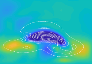
The time evolution of the modes can be visualised in figure 14 on top of the streamwise shear at the wall from the DNS. From these results, we can conjecture a few reasons why the tracking stops. The first reason is that the disturbance did not develop in the simulation, either because of the streak became stable or because another unstable mode with higher amplitude took over. A second reason is the instability encounters a turbulent region downstream. The third reason is the instability appearing in the DNS reaches an amplitude comparable to the streaks, resulting in the stability calculations done over an already significantly disturbed streak. This last option seems to be the case for mode 1, where even though it cannot be followed until the appearance of the turbulent region, traces of it can be observed when looking closer at the shear in between the last station of the mode and the turbulent region. This becomes more evident when we look at the DNS field around this region, as is shown in figure 15. Here, the velocity field is shown at two planes: at the position where the unstable mode 1 was tracked for the last time and at a plane following the instability before the turbulent region. For this last plane, the contours of the unstable mode are also included, which resembles quite well the DNS solution and more importantly, it is predicted before its appearance and before the nucleation of the turbulent spot.
Time-space diagram showing the streamwise shear at different span locations, from (a) to (c),  $z=\{0.059, -0.071, 0.031\}$, corresponding to the span location of the modes shown in figure 9. The black line represents the interface between laminar and turbulent regions, and the coloured markers are the same as in figure 13.

Contours showing zoomed views of the velocity field from DNS. (a,c,e) Plane corresponding to  $Re_x=0.883\times 10^{5}$ and $t=1.92\times 10^{-2}$, which is the last station where mode 1 was tracked (see figures 13 and 14). (b,d,f) Translated plane, $\Delta t=1.2\times 10^{-2}$ and $\Delta x=0.7\Delta t$, with the white contours representing the absolute value of mode 1. Note that for better visualisation of the secondary instability, the streamwise velocity corresponds to the perturbation by subtracting the streamwise velocity at the previous plane.

4.2. Statistical results
4.2.1. Statistics of unstable mode clusters
Let us now move to the results obtained by repeating the previous analysis over all the unstable modes found in a larger streamwise extension and longer time. For this purpose, stability calculations were performed in 70 equidistant planes in the range  $Re_x=[0.2,1.6]\times 10^{5}$, where the upper limit was chosen to be close to the transition location, $\gamma \approx 0.5$, shown in figure 5, while the lower limit was arbitrarily set but corroborated afterwards to be a reasonable choice. The streamwise spacing between two consecutive planes, and therefore the total number of planes, is given by the selection of the time spacing $\Delta t=6\times 10^{-3}$ between stability calculations and along the line $\Delta x /\Delta t=0.7$, where both quantities are based on the results presented in figure 10. We wish to note that the stability calculations are independent of each other and therefore parallelised with no extra implementation. Considering the 70 wall-normal planes and 360 snapshots, the stability computations yielded a total of 152 232 unstable modes.
Following the methodology described in the previous section, the unstable modes are clustered together based on the correlation between their eigenfunctions, where again, each mode can belong to only one cluster. A summary of the clusters is included in table 2 for different correlation thresholds, including the number of clusters corresponding to single modes that could not be correlated with any other unstable mode. For clusters composed of more than one unstable mode, the table also shows the number of them reaching a certain  $N$-factor during their evolution. From the table, we can see the dependence of the results on the correlation threshold, where, as expected, for higher thresholds, the number of uncorrelated modes increases and the number of clusters reaching a certain $N$-factor decreases.
Number of single modes and clusters for different correlation thresholds. For the clusters composed of more than one mode, the number of them reaching a certain  $N$-factor is also included.

Even though there is a dependency on the correlation threshold, whose value remains a free parameter that has to be arbitrarily chosen, the trend and order of magnitude of the results presented in table 2 are fairly insensitive to its choice. In particular, the number of uncorrelated modes is large, representing more than 50 % of the total number of unstable modes independently of the correlation threshold. Before addressing this situation in more detail, we need to comment on one fact of our stability calculations that might be overlooked. The last station for stability analysis was chosen to be close to the average transition position based on the intermittency function, which means that some planes will already contain developed secondary instabilities and mature turbulent spots. This is an unavoidable consequence coming from the spread appearance of instabilities and nucleation of turbulent spots, and for which we did not take any particular action when performing the stability calculations.
As shown before, choosing a lower correlation threshold allows us to follow some instabilities for longer, which can explain the differences between the results for different thresholds, but still not the majority of them. That being the case, we checked whether they were in turbulent regions or not, and an example of this is presented in figure 16. Here, a laminar–turbulent discrimination is shown for a certain snapshot and, on top of that, the unstable modes at the same time instant. It can be seen how most of the uncorrelated modes reside in turbulent regions, while modes that can be correlated to other unstable modes are in laminar ones. In fact, 69.8 % and 60.2 % of the uncorrelated modes reside in turbulent regions when using a correlation threshold of 0.75 and 0.9, respectively. However, less than 1 % of the correlated modes are found in turbulent regions, based on our discrimination. To further characterise the uncorrelated modes, figure 17 shows their conditional distribution, whether they are in laminar or turbulent regions, in terms of their temporal growth rate and their streamwise position. It can be observed how the vast majority of them, either laminar or turbulent, appear near the transition location with relatively low growth rates. The fact that unstable modes in turbulent regions are automatically discarded without the need of any special treatment is a convenient outcome of our algorithm, which works even when a given plane is composed of laminar and turbulent flow. This is a result of the localised nature of the secondary instabilities and that it is possible to detect them before they become appreciable in the flow field distorting the streaks.
Arbitrary snapshot showing the laminar (white) and turbulent (black) regions together with the unstable modes at the same time instant.

Conditional distribution of modes that were not correlated, with a threshold of  $0.75$. Mode distributions according to (a) their growth rate and (b) their streamwise position $Re_x$.

Moving now to the clusters composed of more than one mode, we can see from table 2 that only a fraction of them reaches a significant amplification, namely the  $N$-factor. Figure 18 shows the distribution of the clusters reaching an $N\hbox{-}{\rm factor} >2.5$ according to their initial growth rate, initial streamwise position and their streamwise extension, with the streamwise extension $\Delta Re_x$ defined as the difference between the last and first station of the clusters. The distributions are shown for two correlation thresholds, indicating that they are rather insensitive to its choice. From the first plot, it can be noted how most of the clusters have a relatively small initial growth rate, meaning that if we were to base our analysis on this metric, they would probably be discarded. When comparing the distribution of the initial streamwise position of the clusters, figure 18(b), with the intermittency function in figure 5, there is a good correspondence between the transition region and the appearance of the instabilities, where they start developing just before the intermittency increases and have an emergence peak around the onset of transition. The streamwise extension of the clusters is shown in figure 18(c), which presents the highest variation with the correlation threshold consistent with the fact that a lower threshold enables a longer tracking of the instabilities. In any case, the results are rather robust and also consistent with the outer mode tracking by Hack & Zaki (Reference Hack and Zaki2014) (cf. figure 8), where they were able to follow the unstable mode for $\Delta Re_x=6.4\times 10^4$, which is close to the upper limit of our distribution, but only up to $\Delta Re_x \approx 3.6\times 10^4$ before the instability became apparent in the DNS, a condition where our tracking is doomed to stop and whose value is closer to our distribution peak.
Distribution of clusters satisfying  $N\hbox{-}\text{factor}>2.5$ for different parameters, using two correlation thresholds (CTs). (a) Distribution for the initial temporal growth rate and (b) for the initial $Re_x$ where clusters are detected for the first time, and (c) extension $\Delta Re_x$ of the clusters.

4.2.2. Relation between unstable mode clusters and turbulent spots
So far, we have shown how the emergence and extent of the secondary instabilities has a good correspondence with the transition zone in this flow configuration. We now discuss our efforts to correlate the instabilities with the nucleation of individual turbulent spots. The motivation for this comes mainly from the visual inspection of the flow when plotted together with the instabilities, as shown in supplementary movie 1 available at https://doi.org/10.1017/jfm.2024.433. It can be seen in that time sequence how the nucleation of turbulent spots is generally preceded by secondary instabilities, where our laminar–turbulent criterion was not included to avoid any bias towards the visualisation. By looking at the shear in the animation, it can also be seen that generally before the nucleation events, regions of short streamwise wavelength appear. This is also illustrated in figure 19, where the zoomed view of the shear at the wall shows short wavelength streamwise modulation at three different span locations, which will later break down. The wavelengths of these perturbations are approximately  $\Delta x_1\approx 7.1\times 10^{-3}$, $\Delta x_2\approx 5.9\times 10^{-3}$ and $\Delta x_3\approx 5.2\times 10^{-3}$, giving a wavenumber of the order of that used for the stability calculations.
Shear at the wall at an arbitrary snapshot, where the zoomed view depicts streamwise modulation at three different spanwise locations. Note that the colourmap of the zoomed view has been saturated for better visualisation of the instabilities.

To establish a relation between turbulent spots and instability events, it is first necessary to define when and where a spot is nucleated, since they appear in a range of streamwise positions and in a scattered distribution in time and along the span. To do so, we rely on the laminar–turbulent discrimination described above, in § 3.2. Starting from this binary representation of the field, we find and count the connected pixels of each snapshot, where two pixels are connected if their corners or edges touch. Due to the growth in time of the turbulent spots and the sampling frequency of the snapshots, the connectivity in time between turbulent spots in consecutive snapshots is established by checking the overlap between them and, if there is any, we assume they correspond to the same turbulent spot just convected downstream. After this process, there are still some remaining events that do not fulfil the characteristics of turbulent spots and are therefore discarded. The first type corresponds to single events in time that cannot be connected to any later turbulent spot. The second type corresponds to events that do not have a monotonically growing area.
An example of the tracking of one turbulent spot is presented in figure 20, where the first frame of the time sequence represents the spot nucleation, and whose position and time instant are tabulated together with the other nucleation events. In this dataset, each  $n$ entry is defined as ${T}_{spot}(n)=\{t,x,z\}^n$. The distribution of the turbulent spots nucleation in the streamwise location is presented in figure 21, showing a peak around the transition location ( $\gamma \approx 0.5$), similar to the findings by Nolan & Zaki (Reference Nolan and Zaki2013) for their ZPG case.
Time sequence, from (a) to (c), following one turbulent spot (red contour) after its nucleation. The grey contours represent the streamwise shear at the wall, while the open black contours the interface between laminar and turbulent regions. The time spacing between snapshots is  $\Delta t=2.8\times 10^{-2}$.

Distribution of the turbulent spot nucleation along the streamwise coordinate.

With the evolution history of the instabilities,  ${T}_{inst}$, and the position and time instant where turbulent spots are nucleated, ${T}_{spot}$, we can now move to the connection between these two datasets. Given the fact that it is generally not possible to follow the instabilities after they become noticeable in the DNS within our framework, for an identified nucleation, we are forced to look for instabilities at previous time steps and upstream positions. A schematic of how this search is performed is presented in figure 22(a) for one spot nucleation. In this case, the axes are centred around the nucleation, with the black lines showing the path of the instabilities reaching a certain $N$-factor and that satisfy $|z_{spot} - z_{inst}|<\Delta z$, where $z_{spot}$ is the span position of the turbulent spot nucleation, $z_{inst}$ the instability spanwise position as in (4.2) and $\Delta z=9\times 10^{-3}$ a prescribed tolerance parameter whose value is the same as that used for the mean filter in the laminar–turbulent discrimination (see figure 4). Moreover, this value is close to the spanwise average extension of the instabilities corresponding to $8.8\times 10^{-3}$ with a standard deviation of $1.6\times 10^{-3}$. From this subset of instabilities, we have to decide which ones can be connected to the turbulent spot nucleation. This is decided based on whether they fall into the blue area shown in figure 22 or not, which is defined by three searching parameters: a time interval before the nucleation event $\Delta T$, and a group speed ranging in between $c_1$ and $c_2$. For the example in figure 22, only two instabilities, shown in red, fall in this region and are said to be related to the nucleation event.
Correspondence between instabilities and turbulent spots nucleation. (a) Time-space diagram showing an example of how correspondence is defined for a specific nucleation event centred at  $(0,0)$. The grey contour represents the turbulent region, and the red and black lines depict the instabilities’ evolution, with the stars showing the position where the instability reaches a certain $N$-factor. (b) Correspondence performance, as in (4.6) and (4.7), with filled markers showing the ratio of nucleation events that can be related to instabilities, and open markers the ratio of instabilities that can related to turbulent spots.

The process is then repeated for all the nucleation events appearing after a transient of  $t_{i}=1.2\times 10^{-2}$ to allow the instabilities to develop and before $Re_x=2\times 10^5$, since our last stability calculation station is at $Re_x=1.6\times 10^5$ and, on average, instabilities can be tracked for a $\Delta Re_x \approx 0.3\times 10^5$, as can be seen in figure 18, making futile any attempt to connect them to a nucleation taking place downstream. These constraints leave us with 289 nucleation events, where the performance of correspondence between instabilities and nucleation is defined as
 $$\begin{gather} \mathcal{E}_{spot} = \frac{\text{Nucleations related to instabilities}}{\text{Nucleation events}}, \end{gather}$$
 $$\begin{gather}\mathcal{E}_{inst} = \frac{\text{Instabilities related to nucleation}}{\text{Instabilities}}, \end{gather}$$
where both metrics are dependent on the  $N$-factor of the instabilities. Note that the numerators in the above equations are not necessarily equal because, within our definition, more than one instability can be related to one single turbulent spot nucleation. Figure 22(b) shows these performance metrics as a function of the $N$-factor. These curves correspond to the results using a correlation threshold of $0.85$ to track the instabilities, while for the searching parameters, $\Delta T=0.17$, $c_1=0.65$ and $c_2=0.95$ were chosen. The time interval $\Delta T$ is close to that used by Hack & Zaki (Reference Hack and Zaki2014) for their ZPG case when looking for instabilities before spot nucleation, while the two speeds are based on the stability results of optimal streaks by Brandt et al. (Reference Brandt, Cossu, Chomaz, Huerre and Henningson2003) (cf. figure 5). Results for different parameters are included in Appendix C. The percentage of instabilities that cannot be related to nucleation events, i.e. $1-\mathcal {E}_{inst}$, can be regarded as false-positives, while the nucleation events that cannot be related to instabilities, i.e. $1-\mathcal {E}_{spot}$, as a measure of the false-negatives. By looking at figure 22(b), the trend is quite clear and consistent: for higher $N$-factor, the number of false-positives decreases, meaning that we become more certain that those instabilities will lead to breakdown; however, the number of false-negatives increases, since there are fewer instabilities that can reach higher $N$-factor before they break down. Moreover, the fact that the $\mathcal {E}_{spot}$ tends to 1 as the $N$-factor decreases is further evidence regarding that before a nucleation event, a streak instability is present, in concordance with the results by Hack & Zaki (Reference Hack and Zaki2014).
The two curves in figure 22(b) cross at  $N\hbox{-}\text{factor}\approx 3.3$, reaching a performance of $\mathcal {E}\approx 0.65$. This value is within the range of the single-input-feature prediction by Hack & Zaki (Reference Hack and Zaki2016), where neural networks were trained to classify streaks into two classes: whether they break down or not. However, it is difficult to make a more detailed comparison with their work given that in our approach, most of the streaks that do not break down are already filtered out by the stability calculations. Moreover, their performance was based on a single metric using the total number of streaks, breaking and non-breaking; therefore, we can only conjecture that the breaking and non-breaking streak classification followed the same performance values. Even for their best performance ( $\approx 90\,\%$), this could be problematic for accounting for the false-positive events, i.e. classifying non-breaking streaks as breaking ones. This is due to the imbalance of their test data, where breaking and non-breaking events were not equally distributed, with the latter appearing much more often and representing $99\,\%$ of the dataset. This would imply, for their best performance, a $9.9\,\%$ of false-positives which is an overestimation of the actual data, containing only $1\,\%$ of breaking events.
The last quantity of interest corresponds to the distance from the instabilities to the nucleation events. Here, we wish to emphasise that our  $N$-factor computations are only possible in the streamwise extension where we can track the instabilities, meaning that they can generally experience higher amplification in the DNS before their breakdown. The distance distribution, in terms of $\Delta Re_x$, is presented in figure 23, where the distance is counted from the position where instabilities reach a certain $N$-factor. In this figure, three different $N$-factor values are presented and even though their distributions are within the same range, the trend is clear, where the higher the $N$-factor results in a closer nucleation event.
Distribution of the distance between turbulent spot nucleation and the instability events at the position where they reach a certain  $N$-factor. The dashed lines represent the mean of each distribution.

One stage of the transition process that is not considered in our calculation, and generally in any  $e^N$ criterion, is the receptivity phase, dictating the initial amplitude of the disturbances. This could explain, to some extent, the $N$-factor range where we can correlate instabilities with nucleation events and also the distribution of $\Delta Re_x$ for a given $N$-factor in figure 23. The presence of FST, with the different scales and amplitudes involved, makes the accounting of this phase even more challenging for individual instabilities. To assess the disturbance level inside the boundary layer, the energy spectrum was computed at different positions by taking the Fourier transform of the velocity signal. Figure 24 shows an example of this process for two wall-normal probes at a fixed span and $Re_x$ position. The wall-normal positions were chosen to be in the upper part of the boundary layer, given the appearance of secondary instabilities in lifted low-speed streaks. The red area in this figure corresponds to the range of frequencies of interest for our stability calculations. Interestingly, the disturbance amplitude in this range is only a few orders of magnitude smaller than the dominant low-frequency streaks. Moreover, an almost constant order of magnitude was observed for different $Re_x$, where only low-frequencies showed a noticeable amplification with $Re_x$. This relatively high background noise in the range of interest compares favourably well with the, at a first glance, low $N$-factor shown in figure 22. Moreover, it is plausible that instabilities can reach slightly higher amplification before their breakdown given that, in general, we can only track them up to the position where they become apparent in the DNS.
Energy spectrum at  $Re_x=0.5\times 10^5$ and $z=0$. The black and grey lines correspond to the wall-normal positions $y/\delta ^*(x)=\{2,3\}$, respectively. The red shaded area shows the range of interest for our stability calculations.

5. Conclusions
The present study considered the stability of a boundary layer on a flat plate forced by FST. More specifically, the stability of the streaky base flow was analysed by means of local stability analysis in the temporal framework, whereas the spatio-temporal growth of the instabilities was established through the topological characteristics given by the eigenfunctions of the unstable modes at shifted planes in space and time. This procedure allows us to study the convective evolution of the secondary instabilities along the flat plate while, locally, remaining in the temporal framework. The dataset corresponds to the DNS performed by Durović et al. (Reference Durović, Hanifi, Schlatter, Sasaki and Henningson2024), where realistic experimental flow conditions and a sharp leading edge were considered. The numerous instabilities and turbulent spot nucleation events taking place within the snapshots allow us to statistically assess the relevance of secondary instabilities not only by considering their local growth rates, but also their evolution along the boundary layer.
The linear stability analysis performed on this realistic flow scenario, with its broadband spectrum, is able to recover the localised and scattered nature of the secondary instabilities and their precedence to turbulent spot nucleation. Moreover, in this particular flow case, the visual inspection of the unstable modes shows that they are generally centred around lifted low-speed streaks close to the boundary layer. Our results represent further evidence regarding the important role in transition that secondary instabilities of streaks play in boundary layers forced by FST, where no sign of TS wave secondary instabilities was seen. Certainly, since this work considers only one FST spectrum, it is not possible to rule out other mechanisms that might be of relevance in bypass transition under different FST conditions. With the present data, however, they are expected to be relevant for a small fraction of the nucleation events.
We have presented a way to study the convective evolution of the streak secondary instabilities where we follow the wave packet by performing local stability analysis in subsequent planes shifted in time and in the streamwise direction. Here, we established the topological connections between the different modes at shifted planes from the correlation based on the eigenfunctions, where a high correlation is only obtained for modes at the same span location and presenting the same symmetry. On average, instabilities reaching a significant amplification can be tracked for up to  $\Delta Re_x\approx 0.3\times 10^{5}$. One main benefit of this procedure is that unstable modes with relatively low growth rates are also included in the analysis. By doing so, we observed that large amplification is not only attained to instabilities with high growth rates, but also to instabilities that can sustain their growth in spite of being low. This suggests that by only considering the local growth rate, one could miss some breaking events and at the same time consider instabilities that are not sustained downstream. Another interesting property of the algorithm is its capability to filter out instabilities in already turbulent regions without any extra implementation or flow inspection.
By integrating the temporal growth rate of the instability events, while following the wave packet, we were able to quantify the total amplification of the secondary instabilities during the tracking. It has been shown that the appearance of the instabilities reaching significant amplification ( $N\hbox{-}\text{factor}>2.5$) is well correlated to the onset of transition when contrasted to the intermittency function. Defining a critical $N$-factor value is challenging in this type of flow configuration, when a broadband and evolving spectrum is present inside and outside the boundary layer. Nevertheless, our results suggest that an $N$-factor in the range $[2.5,4]$ is enough to predict the majority of turbulent spot nucleation, while keeping low the number of false positives. Within this range, it is found that breakdown takes place on average $\Delta Re_x\approx {[0.31,0.36]\times 10^{5}}$ after the instabilities reach such amplification. As in most $e^N$-methods, the receptivity phase is not considered in the present work. However, the accounting of the initial disturbance amplitude will likely result in more accurate prediction of the transition onset.
This investigation represents a step forward towards the development of new transition prediction tools in a boundary layer subjected to FST. In this regard, the distribution of the appearance of secondary instabilities together with the distribution of their travel distance before breakdown can be used to model spot nucleation events. For instance, in the work by Kreilos et al. (Reference Kreilos, Khapko, Schlatter, Duguet, Henningson and Eckhardt2016), the position-dependent rate of nucleation events was physically motivated, but without any consideration of the stability of the flow. The distributions mentioned above will certainly depend on the characteristics of the free-stream disturbances, namely the turbulence intensity and the length scales, where it is likely that the appearance of the instabilities will be the most sensitive of them due its dependence to individual unstable streaks in the boundary layer. Therefore, for a full predictive method, it will be necessary to incorporate models regarding the receptivity process to be able to quantify the amplitude and scales of streaks.
Supplementary movie
Supplementary movie is available at https://doi.org/10.1017/jfm.2024.433.
Funding
This work was funded by Vinnova through the NFFP project LaFloDes (grant number 2019-05369); the European Research Council (grant agreement 694452-TRANSEP-ERC-2015-AdG); and the Swedish e-Science Research Centre (SeRC). The computations were performed on resources provided by The National Academic Infrastructure for Supercomputing in Sweden (NAISS) at PDC.
Declaration of interests
The authors report no conflict of interest.
Appendix A. Parameter selection for stability calculations
The stability calculations performed in this work require the choice of some parameters which have an impact on the results and whose final values are presented in table 1. The purpose of this Appendix is to document the studies to decide these parameters.
The first study corresponded to the mesh convergence where we chose the number of  $N_y$ and $N_z$ points along the wall-normal and spanwise directions, respectively. This corresponds to the mesh used for stability calculations, which is different from that in the DNS. However, the base flow was spectrally interpolated from the DNS solutions into the stability mesh. Figure 25 shows the spectrum using different meshes, with panels (a) and (b) showing the variations with $N_y$ and $N_z$, respectively. In both plots, the black markers represent the mesh used in this paper.
Mesh convergence study for the eigenvalue solver, showing the spectrum for different mesh sizes. (a) Number of wall-normal points varied for a fixed  $N_z=500$. (b) Number of span points for a fixed $N_y=44$.

Given that we are solving the temporal problem in the local stability analysis, a streamwise wavenumber  $\alpha$ must be chosen. Its choice was based on the stability results at three consecutive planes, where the most unstable eigenvalue was obtained for a range of wavenumbers. These results are presented in figure 26(a), from which $\alpha =1200$ was chosen. Figure 26(b) shows the spectrum comparison for three different wavenumbers at a fixed plane, with the black markers showing the one used in this work. The choice of a constant $\alpha$ for all our stability calculations could be argued to be one of the strongest simplifications in our process. This is due to the rich disturbance population inside the boundary layer, where, even at a fixed streamwise position and frozen time, different streaks might have different preferences in terms of their stability for different streamwise wavenumbers. Nevertheless, by looking at figure 26(b), it is expected that using a different $\alpha$ in a reasonable range around our choice should not affect the general results of this work.
(a) Maximum temporal growth rate for different streamwise wavenumbers  $\alpha$ at three different planes. (b) Spectra at fixed plane for three different wavenumbers.

The generalised eigenvalue problem in the stability calculations is solved using the function eigs() in MATLAB, which takes advantage of the sparsity of the operators in the system of (3.3). As the eigenvalue problem is large, the algorithm, based on the Arnoldi method, aims to find the  $N$ closest eigenvalues to a prescribed scalar $\sigma$. This scalar is in general complex, which in our formulation, takes the form $\sigma =c\alpha +i10$. Therefore, once a streamwise wavenumber $\alpha$ is selected, the parameter that dictates the real part of $\sigma$ is a user-defined phase speed $c$. The spectra at a fixed plane for different $c$ values in the range of interest for streak secondary instabilities are presented in figure 27. A value of $c=0.7$ was chosen in this work since it captures most of the unstable modes, in addition to being consistent with the phase speed generally reported in the literature for streak instabilities. Varying the imaginary part of $\sigma$ in the range 1–100 did not yield to significant differences in the spectrum, where the same unstable modes were found. However, the computation time for the eigenvalue solver is increased by a factor of $\approx 2$ when using 100 instead of 10.
Spectrum closest to the value  $\sigma =c\alpha +i10$, considering different $c$ values and $\alpha =1200$.

Appendix B. Base flow correlation
The stability analysis performed in this work relies on the parallel flow assumption of the frozen planes. We can justify this assumption based on the weak time dependence of the base flow in the pre-transitional part of the boundary layer, corresponding to a steady two-dimensional (2-D) solution populated by low frequency streaks. Moreover, the secondary instabilities are characterised by a high frequency, relative to the streaks, making this assumption more robust. An example of this time scale difference can be visualised in the spectrum shown in figure 8. If strong variations in consecutive planes where we perform stability analysis were encountered, we would expect their stability to be different as well, which effectively leads to a low correlation of the modes. Therefore, following the modes from their upstream positions serves as a safeguard towards strong variations in the streamwise direction of the base flow. This can be seen from the fact that we are not able to track unstable modes in already turbulent regions.
In any case, the correlation of the base flow in shifted planes could serve as a sanity check regarding the time scale over which the base flow changes while following the modes and also as a further justification of the flow parallel assumption. Therefore, we have computed the correlation of the perturbation DNS field shown in figure 9 using the metric defined in (4.4). Here, the perturbation field is defined as the full DNS solution subtracted by the 2-D steady base flow without FST. Figure 28 shows these results for four different span extensions. The first one corresponding to the full span, while the rest of them by taking only a span extension centred around the unstable modes studied in § 4.1. To avoid the disturbances in the free stream and for all calculations, the wall normal extension was limited to  $y_{max}=4\delta ^*\approx 0.004$, with $\delta ^*$ corresponding to the displacement thickness of the first plane. These results show that the parallel flow assumption is reasonable, given that correlations are consistently close to 1 in the convective frame of reference, moving with the group velocity of the streaks. Moreover, these results are consistent with the time scale over which the instabilities can be tracked.
Correlation of the perturbation base flow shown in figure 9 with planes shifted in time ( $\Delta t$) and streamwise location ( $\Delta x$). In these plots, $z_1=-0.071$, $z_2=0.031$ and $z_3=0.059$, while $\Delta z=0.005$.

Appendix C. Searching parameters
The correspondence between turbulent spot nucleation and secondary instabilities relies on three searching parameters  $c_1$, $c_2$ and $\Delta T$, which were sketched in figure 22(a). Moreover, this correspondence is also dependent on the correlation threshold we choose to track the instabilities. Figure 29 includes the results when varying the different parameters involved, with the black lines in each plot corresponding to the results already shown in figure 22(b).
Parameter studies for the performance of the correspondence between turbulent spot nucleation and instabilities. Open and filled markers for  $\mathcal {E}_{spot}$ and $\mathcal {E}_{inst}$, respectively. In each plot, only one variable from the searching parameters ( $\Delta T$, $c_1$ and $c_2$) and correlation threshold (CT) is changed with respect to the base case (black line) presented in figure 22.

For the searching parameters, the results behave as expected. One can observe that whenever the searching area is increased, either by increasing the time interval  $\Delta T$ or increasing (decreasing) the speed $c_2$ ( $c_1$), both metrics $\mathcal {E}$ defined in (4.6) and (4.7) improve with the same rate, resulting in a shift along the $y$-axis. Still, the largest sensitivity of the performance is seen for the speed $c_1$. Note that this value, together with $c_2$, was chosen based on the results by Brandt et al. (Reference Brandt, Cossu, Chomaz, Huerre and Henningson2003) for optimal streaks, whereas in this flow, a range of wavenumbers is present in the boundary layer. This observation and the results shown in figure 10 could serve as a justification for the use of a lower value.
The dependence on the correlation threshold is also consistent, having different effects in the two metrics  $\mathcal {E}_{spot}$ and $\mathcal {E}_{inst}$, where larger differences are observed for higher $N$-factor. Increasing the correlation threshold represents a less permissive tracking resulting in a lower number of instabilities reaching higher $N$-factor, as is shown in table 2. Therefore, it is not surprising that $\mathcal {E}_{spot}$ drops for higher thresholds since there are fewer instabilities to relate to. However, this reduction in the number of instabilities plays favourably to the metric $\mathcal {E}_{inst}$, since it is defined as the ratio between related and total number of instabilities for a given $N$-factor.


 Open access

