1. Introduction
Elastic elements can serve as auxiliary energy-storage mechanisms that help mechanical and biological systems surpass the instantaneous power limits of their actuators, enabling high-speed or high-intensity motion [Reference Longo, Cox, Azizi, Ilton, Olberding, St Pierre and Patek1–Reference Ilton, Bhamla, Ma, Cox, Fitchett, Kim, Koh, Krishnamurthy, Kuo, Temel, Crosby, Prakash, Sutton, Wood, Azizi, Bergbreiter and Patek3]. As a result, elastic energy storage has been widely exploited to enhance motion speed [Reference Barré, Steinhardt and Wood4–Reference Song, Wang, Lu, Chen and Zhang7], compensate for actuator limitations [Reference Lo and Parslew8–Reference Gallina, Bulian and Mosetti11], and reduce energy losses [Reference Reis and Iida12, Reference Zhang, Zhao, Zhang, Niu and Yan13]. To further improve mechanical energy storage, increasing attention has been directed toward the design of elastic elements tailored to the characteristics of specific actuators [Reference Gatti14–Reference Qing, Guo, Zhu, Chi, Hong, Quinn, Dong and Yin19]. In particular, for electric motors – the most common type of actuator – the maximum load capacity is fixed, and the use of constant-force spring elements can effectively increase the amount of elastic energy stored [Reference Hawkes, Xiao, Peloquin, Keeley, Begley, Pope and Niemeyer20, Reference Jung, Casarez, Lee, Baek, Yim, Chae, Fearing and Cho21], making them a promising solution for efficient energy storage.
To evaluate the energy storage capability of springs, storage efficiency is commonly used as a key performance metric. In particular, the Energy Similarity Index (μ esi ) [Reference Johnson and Rehman22, Reference Ou, Yi, Qaiser, Rehman and Johnson23] provides a quantitative measure of the advantages of constant-force mechanisms (CFMs) (see Figure 1(a)). If the energy storage potential is defined as the product of the maximum force F max and the maximum stroke S max during a quasi-static loading process, then μ esi represents the ratio of the actual stored energy U to this potential. For linear springs without initial residual stress, the storage efficiency μ esi,1 is fixed at 0.5. By contrast, CFMs are well aligned with the goal of maximizing storage efficiency. As a result of their distinctive force–displacement characteristics (Figure 1(b)), which consist of a force rise stage followed by a constant-force stage, they can exploit the full storage potential and thereby achieve a much higher efficiency, with the ideal case reaching μ esi,2 = 1.0.

Figure 1. Advantages of CFM in elastic energy storage. (a) Comparison of energy-storage efficiency and force–displacement relationships between a CFM (dashed line) and a linear spring (solid line). (b) Two distinct phases in the force–displacement curve of the CFM: $\textrm{i}$
) force rise phase,
$\textrm{i}$
) force rise phase, $\textrm{ii}$
) constant force phase.
$\textrm{ii}$
) constant force phase.
Despite these advantages, the spatial and driving costs of the structure have not received sufficient attention in practical design. Commonly used performance indices – such as μ esi , the constant-force ratio factor [Reference Rehman, Qaiser, Ou, Yi and Johnson24], the total deformation maximum (TDM), and the equivalent stress maximum (ESM) – do not fully reflect how force and stroke jointly influence the actual energy storage performance. When comparing two elastic elements under the same stored energy, reduced installation space translates into better spatial efficiency, whereas lower external driving force reduces actuator cost. Both indicators represent practical design considerations in mechanism development.
Traditional CFMs have primarily focused on the mechanical performance within the constant-force segment, whereas optimization aimed at increasing elastic energy storage has been relatively limited. Benefiting from the abrupt stiffness change caused by buckling, slender beam structures [Reference Ma, Chen and Wang25–Reference Bilancia, Geraci and Berselli29] have been demonstrated as an effective approach to achieving long constant-force strokes, thereby offering high potential for energy storage. Nevertheless, in the optimization of such storage mechanisms, insufficient attention has been paid to critical factors such as material stiffness and strength properties, the relationship between mechanism degrees of freedom and deformation, and the resulting stress distribution in the structure – all of which strongly influence the achievable elastic energy.
To address the above issues, this study makes the following contributions. First, focusing on slender-beam-based CFMs, it compares different boundary constraints and demonstrates that the pinned-pinned configuration provides superior elastic energy storage. Building on this configuration, a novel CFM is proposed, featuring both low driving load requirements and a compact structural layout. To further capture the trade-off between energy benefit and mechanical cost, a new evaluation index, EBMCR (Energy Benefit to Mechanical Cost Ratio), is introduced, and multi-objective optimization is performed to refine the structure. Finally, a high-speed catapult is designed based on the optimized results, validating the potential of the proposed design approach for efficient energy storage applications.
The remainder of this paper is organized as follows. Section 2 investigates different boundary conditions and proposes a new CFM design, which is modeled and analyzed using the chained beam constraint model (CBCM). Section 3 conducts multi-objective optimization based on the proposed evaluation index. Section 4 presents the experimental validation, including the development of a catapult device powered by the CFM. Section 5 reports and discusses the experimental results. Section 6 concludes the paper.
2. Mechanism design of the CFM
2.1. The influence of degrees of freedom on CFMs
Boundary conditions play a decisive role in determining the deformation modes, stress distribution, and ultimately the energy storage performance of compliant CFMs.
A typical CFM that exploits the post-buckling behavior of a highly compliant straight beam is illustrated in Figure 2(a). The mechanism consists of a straight beam with length L, width W, and thickness T, together with a fixed frame and a slider. During manufacturing, to minimize assembly requirements, reduce friction, and improve motion accuracy, compliant CFMs are often designed with fixed-fixed (FF) beam ends. Compared with fixed-pinned (FP, Figure 2(b)) and pinned-pinned (PP, Figure 2(c)) configurations, the FF design is inherently more overconstrained and exhibits higher stiffness. However, under the same compressive load, the different deformation modes and stress distributions of these boundary conditions introduce uncertainties in energy storage performance. To clarify the influence of boundary constraints on constant-force stroke and energy storage, this study first conducts a comparative analysis of the three configurations.

Figure 2. Three designs of CFMs with different degrees of freedom: (a) fixed-fixed type with DoF of −2, (b) fixed-pinned type with DoF of −1, and (c) pinned-pinned type with DoF of 0.
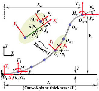
To quantitatively evaluate the energy storage and force–displacement characteristics of CFMs, the chained beam constraint model (CBCM) is adopted for structural modeling. This model has been shown to maintain high accuracy in the large-deflection regime [Reference Chen, Ma, Hao and Zhu30], and the detailed modeling process is provided in Appendix A. The tip load of the beam can be obtained directly or indirectly through the corresponding tip deflection. For all three boundary configurations, the endpoint follows a specific straight-line trajectory (taking the FF case in Figure 3 as an example), which can be expressed as:
 \begin{align}X_{o} &=\textit{S cos} \gamma -L \nonumber \\[2pt] Y_{o}&=\textit{S cos} \gamma\end{align}
The three configurations differ in their boundary conditions at the joints. For the FF case, the rotation at the beam end is restricted to zero:
 \begin{equation}\theta _{o}=0\end{equation}
For the FP case, the end torque of the beam vanishes:
 \begin{equation}M_{o}=0\end{equation}
For the PP case, both end torques, M o and M in , are zero, and moment equilibrium about the origin gives:
 \begin{equation}P_{o}Y_{o}-F_{o}X_{o}=0\end{equation}
By combining Eqs. (1)–(4), the kinetostatic models of the three configurations are established, from which both the strain energy and the overall force–displacement relationships can be derived.

Figure 3. Force analysis of a slender beam structure (FF configuration as an example).
To focus on the effects of boundary constraints, other parameters affecting the force–displacement characteristics are discussed, including beam length L, thickness T, width W, and angle $\gamma$
. Since the mechanism operates in a planar configuration, the beam width W contributes linearly to the load without altering the actual stress distribution or the general trend of the force–displacement curve. In this study, the beam width W is uniformly set to 0.08L.
$\gamma$
. Since the mechanism operates in a planar configuration, the beam width W contributes linearly to the load without altering the actual stress distribution or the general trend of the force–displacement curve. In this study, the beam width W is uniformly set to 0.08L.
As the primary focus of this section is the parameters influencing energy storage efficiency rather than the absolute output force, all parameters are normalized with respect to the geometric dimensions and material properties of the beam. The normalization process is as follows:
 \begin{equation}l = \frac{L}{L} = 1, r = \frac{R}{L}, t = \frac{T}{L}, \gamma = \gamma , \;w = \frac{W}{L}, s = \frac{S}{L}, f = \frac{{F{L^2}}}{{EI}},\end{equation}
where I is the area moment of inertia about the neutral axis, calculated as I = WT 3/12 for a rectangular cross-section; E denotes the Young’s modulus of the material used for the flexible beam segment OA.
In this study, it is assumed that the slender beam structures are assumed to be classified as the highly compliant members in classical column stability theory. Denoting slenderness by $\lambda$
and considering a rectangular cross-section with W ≥ T, the slenderness can be expressed as:
$\lambda$
and considering a rectangular cross-section with W ≥ T, the slenderness can be expressed as:
 \begin{equation}\lambda =\frac{\mu l}{\sqrt{I/D}}=\frac{2\sqrt{3}\mu }{t}\end{equation}
where the slenderness $\lambda$
characterizes the relative flexibility of the beam and the cross-sectional area D is given by D = WT. Larger values of
$\lambda$
characterizes the relative flexibility of the beam and the cross-sectional area D is given by D = WT. Larger values of $\lambda$
indicate a more compliant structure, which is prone to large deflections and post-buckling deformations under compressive loading. In practical terms, when
$\lambda$
indicate a more compliant structure, which is prone to large deflections and post-buckling deformations under compressive loading. In practical terms, when $\lambda$
satisfies Eq. (7), the beam is considered highly compliant, meaning that its strain energy is dominated by bending rather than shear, and shear failure can be neglected within an acceptable error margin. For the FF, FP, and PP configurations, the corresponding length factors μ are 0.5, 0.7, and 1.0, respectively.
$\lambda$
satisfies Eq. (7), the beam is considered highly compliant, meaning that its strain energy is dominated by bending rather than shear, and shear failure can be neglected within an acceptable error margin. For the FF, FP, and PP configurations, the corresponding length factors μ are 0.5, 0.7, and 1.0, respectively.
 \begin{equation}\lambda \geq \lambda _{cr}=\sqrt{\frac{\pi ^{2}E}{\sigma _{P}}}\end{equation}
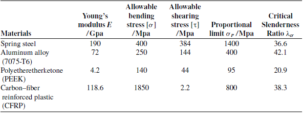
where σ
P
denotes the proportional limit of the material. Based on the material parameters commonly used in compliant mechanism design (see Appendix B), and taking the FF configuration as a reference, the range of thickness T is set to T $ \lt $
0.017 when λ
$ \lt $
0.017 when λ $ \gt $
100.
$ \gt $
100.
Although previous studies [Reference Ma, Chen and Wang25] have shown that the thickness T has no effect on the force–displacement characteristics of FF structures, for completeness it is also considered in the FP and PP configurations. Figure 4 illustrates the variations of the force and displacement curves at $\gamma$
= 80° for thickness values of T = 0.001, 0.006, 0.011, and 0.016. The results indicate that the four curves corresponding to each configuration nearly overlap (Figure 4(a)), with discrepancies within 0.25% (Figure 4(b)). This confirms that, regardless of boundary conditions, the force–displacement characteristics of these structures are essentially independent of the beam thickness.
$\gamma$
= 80° for thickness values of T = 0.001, 0.006, 0.011, and 0.016. The results indicate that the four curves corresponding to each configuration nearly overlap (Figure 4(a)), with discrepancies within 0.25% (Figure 4(b)). This confirms that, regardless of boundary conditions, the force–displacement characteristics of these structures are essentially independent of the beam thickness.

Figure 4. Influence of beam thickness t on the force–displacement characteristics of the three configurations. (a) Nondimensionalized force–displacement relationship of three CFMs with t varying from 0.001 to 0.016. (b) Deviation when the effect of t is neglected.
The effect of $\gamma$
is examined with T = 0.005 and
$\gamma$
is examined with T = 0.005 and $\lambda$
= 692.8μ (μ = 1, 0.7, and 0.5 for FF, FP, and PP, respectively). Nondimensionalized force f and energy e are evaluated with respect to displacement s for
$\lambda$
= 692.8μ (μ = 1, 0.7, and 0.5 for FF, FP, and PP, respectively). Nondimensionalized force f and energy e are evaluated with respect to displacement s for $\gamma$
varying from 50° to 90°. Results are shown in Figure 5, where colors and symbols denote different
$\gamma$
varying from 50° to 90°. Results are shown in Figure 5, where colors and symbols denote different $\gamma$
. The black solid line represents loci of truncation points under specific allowable stresses σ
i
(i = 1, 2, 3, 4), with σ
1
$\gamma$
. The black solid line represents loci of truncation points under specific allowable stresses σ
i
(i = 1, 2, 3, 4), with σ
1 $ \lt $
σ
2
$ \lt $
σ
2 $ \lt $
σ
3
$ \lt $
σ
3 $ \lt $
σ
4. Numerical values are listed in Table I, referenced to the critical buckling stress σ
cr,PP of the PP case. As shown in Figures 5(a)–(c), the slopes of the force–displacement curves in the constant-force stage change from negative to positive as
$ \lt $
σ
4. Numerical values are listed in Table I, referenced to the critical buckling stress σ
cr,PP of the PP case. As shown in Figures 5(a)–(c), the slopes of the force–displacement curves in the constant-force stage change from negative to positive as $\gamma$
increases.
$\gamma$
increases.
The red circles in Figures 5(a)–(c) mark the dimensionless critical buckling loads, which increase with $\gamma$
. At
$\gamma$
. At $\gamma$
= 90°, the critical buckling load P
cr
is given by Euler’s formula:
$\gamma$
= 90°, the critical buckling load P
cr
is given by Euler’s formula:
 \begin{equation}P_{cr}=\frac{\pi ^{2}EI}{\left(\mu L\right)^{2}}\end{equation}
For $\gamma$
≠ 90°, buckling occurs once the resultant axial force P (resultant force of load F plus reaction force F
r
) reaches P
cr
, as illustrated in Figure 6. The critical driving force F
cr
in the loading direction is obtained from the following equation:
$\gamma$
≠ 90°, buckling occurs once the resultant axial force P (resultant force of load F plus reaction force F
r
) reaches P
cr
, as illustrated in Figure 6. The critical driving force F
cr
in the loading direction is obtained from the following equation:
 \begin{equation}F_{cr}=P_{cr}sin\,\gamma =\frac{\pi ^{2}EI}{\left(\mu L\right)^{2}}sin\,\gamma\end{equation}
Figures 5(d)–(f) present dimensionless strain energy under identical allowable stresses (solid black line). The dashed line corresponds to energy at $\gamma$
= 90°. The near coincidence of solid and dashed lines indicates that, for a given maximum bending stress, the effect of
$\gamma$
= 90°. The near coincidence of solid and dashed lines indicates that, for a given maximum bending stress, the effect of $\gamma$
on strain energy is negligible. To quantify this, mean strain energy values ē and their standard deviations (shown as shaded ±1σ bands) were computed across four allowable stress levels, as illustrated in Figure 7. Results show that the FP configuration consistently yields the lowest energy and the largest angular variation (max error ±5.6%), while the PP configuration shows the smallest variation (max error
$\gamma$
on strain energy is negligible. To quantify this, mean strain energy values ē and their standard deviations (shown as shaded ±1σ bands) were computed across four allowable stress levels, as illustrated in Figure 7. Results show that the FP configuration consistently yields the lowest energy and the largest angular variation (max error ±5.6%), while the PP configuration shows the smallest variation (max error $ \lt $
±0.14%). These results were obtained using a displacement-increment approach with linear interpolation to specific stress levels. Smaller increments bring computed stresses closer to target values, improving accuracy.
$ \lt $
±0.14%). These results were obtained using a displacement-increment approach with linear interpolation to specific stress levels. Smaller increments bring computed stresses closer to target values, improving accuracy.
Table I. Allowable bending stress reference values (Material: E = 118.6 GPa).


Figure 5. Influence of beam angle γ on the nondimensionalized force–displacement and energy-displacement characteristics of the three configurations: (a) FF, (b) FP, and (c) PP for force–displacement; (d) FF, (e) FP, and (f) PP for energy-displacement.

Figure 6. Loading conditions of the beam at the critical buckling state.

Figure 7. Mean strain energy ē calculated over four allowable stress levels, with shaded bands representing ±1 standard deviation.
It should also be noted that the FF and FP configurations impose more stringent failure conditions than the PP configuration, since maximum shear forces at fixed ends require additional shear strength verification.
In summary, the PP configuration provides the most favorable balance between stroke length, energy efficiency, and structural reliability. It offers the longest relative stroke, alleviates shear requirements, and reduces both spatial and driving costs. Consequently, the PP configuration is adopted for the subsequent design and optimization of constant-force energy storage mechanisms.
2.2. Design of a new CFM based on the PP configuration
Based on the PP configuration, a new CFM is proposed, as illustrated in Figure 8(a). The mechanism consists of three slender beams, OA, with length L, distributed symmetrically and inclined at an angle $\gamma$
to the horizontal plane, together with a rigid link, AB, of length R. Under a vertical external load F, the mechanism deforms and the upper frame translates along the dashed trajectory. The maximum footprint of the mechanism during deformation is represented by the diagonal length L
d
[Reference Ma, Chen and Wang25].
$\gamma$
to the horizontal plane, together with a rigid link, AB, of length R. Under a vertical external load F, the mechanism deforms and the upper frame translates along the dashed trajectory. The maximum footprint of the mechanism during deformation is represented by the diagonal length L
d
[Reference Ma, Chen and Wang25].

Figure 8. Design of the PP-type CFM: (a) schematic diagram of the design principle; (b) improved gear-beam structure.
Unlike the PP configuration discussed in Section 2.1, the proposed mechanism incorporates an eccentric gear pair, which introduces the rigid segment AB perpendicular to the beams, as shown in Figure 8(b). The eccentric gear and the concentric gear, with rotation centers O and B, respectively, form two pivotal constraints of the mechanism. The rigid link AB of length R ensures that the deformation of segment OA avoids directional uncertainty caused by buckling [Reference Sen, Mohan and Ananthasuresh31]. This geometric determinacy also prevents computational errors in CBCM programming or finite element analysis, where incorrect modal orders may otherwise arise. Although such issues could be mitigated by buckling analysis or introducing perturbations based on low-order mode shapes, those approaches are relatively cumbersome.
Since the bending moment near points O and B is minimal, and the beam length is much larger than the local gear-beam contact length, the beam’s deformation and load transmission are hardly affected by the presence of the gears. Validation confirms that a sufficiently small R produces negligible influence on the force–displacement characteristics (see Appendix C). Therefore, R is uniformly set to 0.005L throughout this study.
The use of gears also ensures synchronous deformation of the symmetrically distributed beams. To prevent out-of-plane twisting, the widths of the two beams on the left side are set to half the width of the single beam on the right side, and the right-side beam is positioned equidistantly between the two left-side beams. This configuration therefore provides a compact, deterministic, and efficient structural basis for the optimization of CFMs.
3. Optimization of CFM
3.1. Formulation of optimization objectives
To enhance the energy storage capability of the CFM, this section considers structural optimization from two perspectives: reducing mechanical cost and improving loading efficiency.
The first objective, representing mechanical cost, is defined through a dimensionless index termed the Energy Benefit to Mechanical Cost Ratio (EBMCR):
 \begin{equation}\textit{EBMCR}=\frac{U}{F_{max}L_{d}}\end{equation}
Here, L d denotes the diagonal length of the maximum footprint rectangle of the mechanism, and U represents the strain energy stored in the structure. A higher EBMCR value indicates minimized costs associated with external driving force and spatial footprint, while maximizing elastic energy storage.
However, two mechanisms with the same EBMCR value may differ in terms of force fluctuations, which in turn leads to differences in relative stroke. In other words, the more stable the constant-force effect, the shorter the required loading stroke. To capture this effect and further improve storage efficiency, the relative constant-force stroke s CF is adopted as the second optimization objective:
 \begin{equation}s_{CF}=\frac{S_{CF}}{L_{d}}\end{equation}
where S CF denotes the maximum constant-force stroke under a specified force fluctuation tolerance ξ f . The fluctuation error ξ f is defined as:
 \begin{equation}\xi _{f}=max\left(\frac{\left| F-F_{t}\right| }{F_{t}}\right)\end{equation}
where F t is the mean value of the force in the constant-force region. If the maximum external force in the loading process is denoted as Fmax and the minimum external force is F min , then F min can be derived from Fmax and ξ f . Furthermore, the average output force F t during the constant-force stage can be obtained as:
 \begin{equation}F_{t}=\frac{F_{max}-F_{min}}{2}\end{equation}
3.2. Multi-objective optimization
This section performs multi-objective optimization of the proposed mechanism. The optimization process combines the NSGA-II algorithm [Reference Deb, Pratap, Agarwal and Meyarivan32] with the CBCM model. As one of the most widely used multi-objective evolutionary algorithms, NSGA-II employs nondominated sorting and crowding distance mechanisms to maintain diversity while ensuring convergence. Owing to these advantages, it has been extensively applied in mechanical design problems [Reference Lin, Luo and Tong33–Reference Zhu, To, Zhu, Li and Huang35]. Using MATLAB, the two optimization objectives described in Section 3.1 are solved, and the results are presented in the form of Pareto solution sets.
It should be noted that although the thickness T was shown in Section 2.1 to have a negligible influence on the force–displacement characteristics, it has a significant impact on bending stress and thus on the amount of stored energy. Therefore, thickness T and loading angle $\gamma$
are selected as the design variables in the optimization process. The optimization problem can be formulated as follows:
$\gamma$
are selected as the design variables in the optimization process. The optimization problem can be formulated as follows:
 \begin{align} \textit{Objectives} &\begin{cases} max\colon g_{1}=\textit{EBMCR}\nonumber\\ max\colon g_{2}=s_{CF} \end{cases}\\ s.t. &\begin{cases} T_{l}\lt T\lt T_{u}\\ \gamma _{l}\lt \gamma \lt \gamma _{u}\\ \sigma _{max}\lt \left[\sigma \right] \end{cases}\end{align}
where T
l
, T
u
, and $\gamma$
l
,
$\gamma$
l
, $\gamma$
u
represent the lower and upper bounds of parameters T and
$\gamma$
u
represent the lower and upper bounds of parameters T and $\gamma$
, respectively.
$\gamma$
, respectively.
During the evaluation of individual fitness, the external load is applied using displacement increments. Each incremental step requires solving the CBCM equations. As the displacement increases, once the maximum bending stress σ max exceeds the allowable bending stress [σ], or the physical displacement limit (set as the beam length L) is reached, the maximum displacement S max is uniquely determined. After each generation, information for the corresponding parameter set – including force–displacement data, maximum lateral deformation (for computing L d ), strain energy, and maximum displacement – is recorded. Furthermore, the constant-force stroke is extracted by traversing the force–displacement sequence. Because the structural configuration now includes the additional parameter R, the corresponding kinetostatic model is reformulated, as detailed in Appendix A.
In the optimization, carbon-fiber-reinforced polymer (CFRP) is chosen as the structural material, with a beam length L = 300 mm and a maximum bending stress of 1.85 GPa. Based on preliminary calculations, the thickness is varied within 0.1–6 mm, and the loading angle $\gamma$
within 50°–130°. In the CBCM formulation, each beam is discretized into 20 segments.
$\gamma$
within 50°–130°. In the CBCM formulation, each beam is discretized into 20 segments.
The NSGA-II algorithm is employed with the following settings: a population size of 200, a maximum of 200 generations, simulated binary crossover (SBX) with a distribution index of 15 and a crossover probability of 0.9, and polynomial mutation with a probability of 0.1 and a distribution index of 15. To ensure robustness of the results, the optimization is repeated five times independently. The final Pareto front is obtained by merging all nondominated solutions from these runs and applying a secondary filtering step. To avoid wasted computational time due to premature convergence, the hypervolume (HV) metric [Reference Lin, Luo and Tong33] is adopted as a criterion to evaluate both the convergence and the diversity of solutions.
The optimization results are shown in Figure 9. Figure 9(a) presents the Pareto front, where the EBMCR objective g
1 is plotted on the horizontal axis and the relative constant-force stroke objective g
2 on the vertical axis. The Pareto front reveals a trade-off between EBMCR and s
CF
, exhibiting a monotonic decrease: as s
CF
decreases from 0.46 to 0.30, EBMCR increases from 0.58 to 0.81. To balance both objectives without significant loss of either, the two objectives are normalized (Eq. (15)), and the final solution is chosen by maximizing their product, i.e., max( $\overline{g}$
1,
$\overline{g}$
1, $\overline{g}$
2).
$\overline{g}$
2).
 \begin{equation}\overline{g}_{1}=\frac{g_{1}}{max\,\left(g_{1}\right)},\overline{g}_{2}=\frac{g_{2}}{max\,\left(g_{2}\right)}\end{equation}
This criterion geometrically corresponds to selecting the point on the normalized Pareto curve that maximizes the rectangular area spanned with the origin (0,0). Mathematically, it is equivalent to a geometric mean, reducing sensitivity to extreme values on the Pareto front and reflecting the coordination between the two objectives.
Table II. Optimization results for different characteristic dimensions.


Figure 9. Structural optimization results: (a) Pareto front obtained using the NSGA-II algorithm and the strategy for selecting the optimal solution; (b) Pareto solution set and the optimal parameters in this study.
Figure 9(b) illustrates the optimized Pareto set. The star marker denotes the optimal design parameters, $\gamma$
= 113.08° and T = 1.68 mm, corresponding to g
1 = 0.75 and g
2 = 0.44. To further validate the robustness of the optimization, the same procedure is repeated for mechanisms with different primary dimensions L, and the results are summarized in Table II. It can be observed that although the characteristic dimension L
d
varies from 10 to 500 mm, the optimized values of both objectives change only slightly. This demonstrates that the proposed evaluation index exhibits excellent scale independence, making it applicable for guiding the design of mechanisms across different size ranges.
$\gamma$
= 113.08° and T = 1.68 mm, corresponding to g
1 = 0.75 and g
2 = 0.44. To further validate the robustness of the optimization, the same procedure is repeated for mechanisms with different primary dimensions L, and the results are summarized in Table II. It can be observed that although the characteristic dimension L
d
varies from 10 to 500 mm, the optimized values of both objectives change only slightly. This demonstrates that the proposed evaluation index exhibits excellent scale independence, making it applicable for guiding the design of mechanisms across different size ranges.
3.3. Validation of optimization results
To verify the effectiveness of the optimization, a CFM was designed and fabricated using parameters close to the optimal solution ( $\gamma$
= 113.08, T = 1.5 mm, L = 300 mm), as shown in Figure 10(a). In the prototype, the OA beams were made of unidirectional carbon-fiber-reinforced polymer (CFRP), with all cross-sections oriented perpendicular to the fiber direction. The Young’s modulus of the CFRP was 118.6 GPa. To enable adjustment of the loading angle
$\gamma$
= 113.08, T = 1.5 mm, L = 300 mm), as shown in Figure 10(a). In the prototype, the OA beams were made of unidirectional carbon-fiber-reinforced polymer (CFRP), with all cross-sections oriented perpendicular to the fiber direction. The Young’s modulus of the CFRP was 118.6 GPa. To enable adjustment of the loading angle $\gamma$
, four idler gears were incorporated into the system. All gears and the supporting frame were fabricated from polylactic acid (PLA) using 3D printing. The gears were press-fitted to the beams, and the complete assembly was formed by combining the base, moving components, and idlers. The detailed structural parameters are listed in Table III, where m
1 and m
2 denote the modules of the two gear types, and Z
1 and Z
2 their corresponding numbers of teeth.
$\gamma$
, four idler gears were incorporated into the system. All gears and the supporting frame were fabricated from polylactic acid (PLA) using 3D printing. The gears were press-fitted to the beams, and the complete assembly was formed by combining the base, moving components, and idlers. The detailed structural parameters are listed in Table III, where m
1 and m
2 denote the modules of the two gear types, and Z
1 and Z
2 their corresponding numbers of teeth.
Figure 10(b) shows the experimental platform used to measure the force–displacement characteristics of the mechanism. The device under test was placed horizontally, with one end connected to a force sensor (GJBLS-I) fixed to the platform and the other end attached to a linear motion stage (FSL40) driven by a stepper motor. The displacement of the mechanism was measured using a laser displacement sensor (LJ-X8080, KEYENCE), which scanned the position of the moving stage. The two signals were processed through a data acquisition converter and transmitted to a computer via serial communication, enabling synchronous acquisition of the force and displacement data.
To further validate the kinetostatic model and the experimental measurements, finite element simulations were performed in Abaqus 2022. The flexible beam was discretized into 1500 linear beam elements (B21), and geometric nonlinearity (Nlgeom = ON) was enabled to capture large deflection effects. A static general step (Static, General) was used, in which the prescribed end displacement was incrementally applied to obtain the force–displacement response as well as the evolution of bending stress. The deformation process is illustrated in Figure 10(c), where configurations (i)–(vi) correspond to displacements of point B (defined in Figure 8) of 0, 33.2, 66.2, 99.2, 132.8, and 165.8 mm, respectively.
Table III. Design parameters of the prototype.


Figure 10. Structural design and experimental validation: (a) prototype of the constant-force energy storage mechanism; (b) experimental testing platform; (c) deformation results of the CFM in Abaqus simulations; (d) comparison among simulation results, kinetostatic model calculations, and experimental results.
The comparison of experimental, model-based, and simulation results is presented in Figure 10(c). The horizontal axis represents displacement (mm), and the vertical axis represents load (N). Experimental results are plotted as circles with error bars, the kinetostatic model predictions as curves with “X” markers, and the finite element simulations as curves with triangular markers. The three results exhibit good agreement. Under the condition of a unilateral fluctuation error ξ
f $ \lt $
2.6%, the measured constant-force stroke accounted for 38.2% of s
CF
, corresponding to a stroke length of 124.9 mm relative to the footprint size L
d
= 326.2 mm. Within the constant-force region, the average output force was F
t
= 67.68 n (for a beam width of 24 mm). These results confirm the accuracy of both the kinetostatic model and the optimization strategy, demonstrating the feasibility of the PP-based CFM in practice.
$ \lt $
2.6%, the measured constant-force stroke accounted for 38.2% of s
CF
, corresponding to a stroke length of 124.9 mm relative to the footprint size L
d
= 326.2 mm. Within the constant-force region, the average output force was F
t
= 67.68 n (for a beam width of 24 mm). These results confirm the accuracy of both the kinetostatic model and the optimization strategy, demonstrating the feasibility of the PP-based CFM in practice.
4. Application of the constant-force energy storage mechanism in a high-speed catapult
To demonstrate the advantage of the proposed design method in terms of energy storage efficiency, we designed a high-speed catapult based on the CFM and compared it with a linear spring. The experimental process is illustrated in Figure 11(a). During the loading phase, both mechanisms were subjected to an identical external force F, which was applied to the spring via a rope, causing it to store energy. The deformation of the spring was fixed by a latch mechanism. Once the latch was released, the catapult entered the ejecting phase, during which it accelerated the projectile in the horizontal plane. Upon reaching the design stroke, the catapult began to decelerate, causing the separation of the projectile and completing the launch. In the experiments, a tennis ball was used as the projectile and was supported by a compliant gripper during acceleration. The inertial force maintained contact between the ball and the gripper with minimal friction, resulting in negligible energy loss. The gripper geometry was identical for both catapult prototypes, as shown in Appendix D. The motion of the projectile was recorded using a camera (1280 × 720 pixels, 480 frames per second), and the launch velocity was subsequently determined through post-processing analysis.

Figure 11. Comparison between constant force and linear-spring-based catapult mechanisms. (a) Catapult mechanisms based on a CFM and a linear spring, and their corresponding ejection processes. (b) Energy-displacement and force–displacement curves under quasi-static testing for both spring types. (c) Prototypes of the two catapults: ( $\textrm{i}$
) linear-spring catapult and (
$\textrm{i}$
) linear-spring catapult and ( $\textrm{ii}$
) constant-force catapult. (d) Experimental comparison of the two mechanisms in ejecting a standard tennis ball.
$\textrm{ii}$
) constant-force catapult. (d) Experimental comparison of the two mechanisms in ejecting a standard tennis ball.
To ensure a fair comparison, the external loading and stroke of both the constant force and linear springs were maintained at the same levels. Specifically, an external force of 70 N was applied, and the beam width of the CFM was set to 6 mm (four beams in total). The linear spring was selected from an industrial product series based on its stiffness calculation. Two parallel stretch spiral springs with a large diameter of 12 mm, a small diameter of 1.2 mm, and a length of 96 mm were chosen, resulting in a stiffness of 0.367 N/mm and an initial preload of 8.8 N. The force–displacement curves of the CFM and the linear spring system are shown in Figure 8(b), where both exhibit the same maximum external force at a stroke of 170 mm.
For a fair assessment of the energy-storage performance, the tennis balls and all accelerated components (including the gripper) were mass-matched between the two prototypes, eliminating bias from ancillary moving mass. After measurement, the lumped mass of the gripper and all other accelerated components (denoted as m gr,CFM ) is 63.8 g, while the mass of the linear spring catapult (m gr,LM ) is 65.1 g, showing close agreement. Based on the energy curves in Figure 11(b), the constant force catapult can store 11.2 J of energy within a 170 mm displacement, while the linear spring catapult stores 6.8 J. When frictional and other resistive forces, as well as the intrinsic mass of the spring, are ignored, the theoretical kinetic energy E k ∗ achievable by a 66-mm-diameter, 56.4-g tennis ball can be calculated for the two mechanisms using the following equations:
 \begin{equation} {E}^{*}_{k,1}=11.2 \, {\rm J}, \cdot \frac{m_{ball}}{m_{ball}+m_{gr,CFM}}=5.25 \, {\rm J}, {E}^{*}_{k,2}=6.8 \, {\rm J}, \cdot \frac{m_{ball}}{m_{ball}+m_{gr,LM}}= 3.16 \, {\rm J}\end{equation}
Here, ${E}^{*}_{k,1}$
and
${E}^{*}_{k,1}$
and ${E}^{*}_{k,2}$
denote the theoretical kinetic energy of the catapult based on the CFM and the linear spring, respectively.
${E}^{*}_{k,2}$
denote the theoretical kinetic energy of the catapult based on the CFM and the linear spring, respectively.
Figure 11(c) illustrates the prototypes of the two catapults, and the final experimental results are presented in Figure 11(d), where the constant force catapult demonstrates significantly better performance than the linear spring catapult. The tennis ball achieved an initial velocity of 10.36 m/s (± 0.2 m/s) with the constant force catapult, while the linear spring catapult resulted in a lower initial velocity of 7.72 m/s (± 0.15 m/s). The time intervals between each position in the figure are 1/60 s. Based on the conversion in Eq. (17), the actual kinetic energy E k of the ball in the constant force and linear spring catapults are 3.03 J and 1.68 J, respectively.
 \begin{equation}E_{k}=\frac{1}{2}mv_{0}^{2}\end{equation}
where m denotes the mass of the launched object, and v 0 represents its initial velocity at the moment of release.
According to Eq. (18), the energy conversion efficiencies η E for the two mechanisms are 57.7% and 53.2%, respectively.
 \begin{equation}\eta _{E}=\frac{E_{k}}{{E}^{*}_{k}}\end{equation}
The efficiency difference is attributed not only to the different friction coefficients but also to the assumption of neglecting the mass of the springs. The linear spring, made of 304 stainless steel, has a mass of 50.5 g, while the CFRP spring in the CFM weighs only 16.3 g. In summary, under the same maximum external load, the CFM offers a significant energy storage advantage over the linear spring mechanism in catapult design.
5. Results and discussions
Through optimization of the two objectives, the proposed CFM achieves improved performance in both mechanical cost and loading efficiency. To further highlight the advancement of the optimization strategy, comparisons are made with existing mechanisms in terms of EBMCR and relative constant-force stroke.
The comparison of EBMCR is shown in Figure 12(a). The black squares represent the results of other studies, plotted with respect to the characteristic dimension L d , which reflects the footprint of the mechanism. The blue “X” markers denote the theoretical optimization results obtained in this study across different scales, as reported in Table III. The black dashed line indicates the average EBMCR value (0.75 ± 0.004) from Table III, while the shaded region below it represents the design domain achievable by the present method. The proposed catapult prototype is marked with a red star. The results clearly demonstrate that, for designs relying on energy storage to enable rapid motion, the proposed method provides theoretical advantages across a wide range of scales. The experimental validation using the catapult further confirms the effectiveness of the optimization approach.

Figure 12. EBMCR and constant force stroke performance of the proposed CFM. (a) EBMCR comparison across different scales [Reference Bates, Gerig, Avitia, Waldvogel, Legesse, Washington and Bhounsule6, Reference Hawkes, Xiao, Peloquin, Keeley, Begley, Pope and Niemeyer20, Reference Jung, Casarez, Lee, Baek, Yim, Chae, Fearing and Cho21, Reference Noh, Kim, An, Koh and Cho37–Reference Lo and Parslew43]. (b) Comparison of constant force indicators for different types of CFMs [Reference Johnson and Rehman22, Reference Ma, Chen and Wang25–Reference Tolman, Merriam, Howell, Jutte and Kota27, Reference Bilancia, Geraci and Berselli29, Reference Tolman, Merriam and Howell44–Reference Lan, Yang and Wu49].
The proposed optimization method also shows clear benefits in enhancing the relative constant-force stroke s CF . Figure 12(b) compares the CFM designed in this study with other existing mechanisms in terms of force fluctuation error ξ f and relative constant force stroke s CF . The prior studies on CFMs are categorized according to the classification standard from reference [Reference Ling, Ye, Feng, Zhu, Li and Xiao36]. Circles represent designs achieved via topology optimization (denoted by “T”), triangles represent designs utilizing beam buckling effects (denoted by “B”), and squares represent designs exploiting kinematic limb singularity (denoted by “K”). Red markers indicate designs obtained via direct zero-stiffness configuration (denoted as “direct”), while blue markers indicate those obtained using stiffness combination configuration (denoted as “combination”). The red star represents the prototype developed in this study, which belongs to the “B-direct” category. The results indicate that, compared to stiffness combination configurations, CFMs designed with direct zero stiffness configuration exhibit a larger constant force displacement range. The design method proposed in this study achieves an improvement in the constant force stroke while maintaining a controlled fluctuation error, with s CF reaching 38.2% and the constant force stroke approaching 125 mm.
These findings highlight the scalability and generality of the proposed method, providing a robust foundation for practical applications of CFMs.
6. Conclusion
This study proposed a novel design method for CFMs aimed at enhancing elastic energy storage efficiency by addressing both mechanical cost and loading efficiency. A new dimensionless index, the Energy Benefit to Mechanical Cost Ratio (EBMCR), was introduced, and a multi-objective optimization framework was developed by combining NSGA-II with the chained beam constraint model (CBCM).
Comparative analysis of different boundary conditions demonstrated that the pinned-pinned (PP) configuration provides the most favorable balance between stroke length, energy efficiency, and structural reliability. Parametric studies further showed that beam thickness has negligible influence on force–displacement characteristics, while the loading angle plays a critical role. Multi-objective optimization yielded Pareto-optimal solutions, with the final design (γ ≈ 113, T ≈ 1.7 mm) validated by finite element simulations and experimental tests. Notably, the optimized prototype achieved an EBMCR of 0.75 and realized a constant-force stroke covering 38% of the total displacement under a fluctuation error below 2.6%, confirming both the effectiveness of the proposed index and the robustness of the design method.
To demonstrate practical applicability, a high-speed catapult was designed using the optimized CFM and compared against a linear-spring counterpart. The prototype exhibited superior performance, achieving a longer constant-force stroke, higher stored energy, and improved energy conversion efficiency. These results confirm the advantages of CFMs in high-performance energy storage applications.
Overall, this work provides a systematic framework for the design, optimization, and application of CFMs. Future research will extend this approach to dynamic loading conditions, fatigue and reliability analysis, and the integration of advanced materials and metamaterial-inspired structures, thereby broadening the potential of CFMs in robotics and other energy-critical systems.
Author contributions
The research concept was from Yehui Wu, Bo Li, and Fulei Ma. Material preparation, data collection, and analysis were performed by Yehui Wu, Wentao Ma, and Yang Yu. Yehui Wu wrote the first draft of the manuscript. Ruiyu Bai and Guimin Chen contributed to the revision and improvement of the manuscript. All authors read and approved the final manuscript.
Financial support
This work is supported by the National Natural Science Foundation of China under Grant No. 52475030 and No. 52575035.
Competing interests
We declare that we have no financial and personal relationships with other people or organizations that can inappropriately influence our work; there is no professional or other personal interest of any nature or kind in any product, service, and/or company that could be construed as influencing the position presented in the manuscript entitled “Enlarging Elastic Energy Storage via a Constant Force Mechanism.”
Ethical approval
Not applicable.
Appendix A. Kinetostatic model of CFMs
In the CBCM model, the straight beam is divided into N segments as shown in Figure A1. Initially, the beam forms an angle $\gamma$
at the fixed hinge O1, which transitions to a deformed angle θ
1 as point ON + 1 undergoes a displacement S. At this point, the concentrated load at B is resolved into a force P
O
, a force F
O
and a moment M
O
. These components are represented in the global coordinate system by their position (X
O
, Y
O
) and orientation θ
O
. Therefore, there are 6(N + 1) parameters to be determined.
$\gamma$
at the fixed hinge O1, which transitions to a deformed angle θ
1 as point ON + 1 undergoes a displacement S. At this point, the concentrated load at B is resolved into a force P
O
, a force F
O
and a moment M
O
. These components are represented in the global coordinate system by their position (X
O
, Y
O
) and orientation θ
O
. Therefore, there are 6(N + 1) parameters to be determined.
To achieve numerical solutions, we established constraint equations equal in number to the unknown variables. First, the load and displacement parameters of all segments are normalized to eliminate scale differences as follows:
 \begin{align}p_{i}&=\frac{P_{i}L^{2}}{N^{2}EI},f_{i}=\frac{F_{i}L^{2}}{N^{2}EI},m_{i}=\frac{M_{i}L}{EI},\lambda _{i}=\frac{N{{\Lambda}} _{i}}{L},\delta _{i}=\frac{N{{\Delta}} _{i}}{L},\alpha _{i}=\alpha _{i},l=\frac{NL}{L}=N, \nonumber\\[2pt]r&=\frac{NR}{L},p_{o}=\frac{P_{o}L^{2}}{N^{2}EI},f_{o}=\frac{F_{o}L^{2}}{N^{2}EI},m_{o}=\frac{M_{o}L}{NEI},x_{o}=\frac{NX_{o}}{L},y_{o}=\frac{NY_{o}}{L},\theta _{o}=\theta _{o}\end{align}
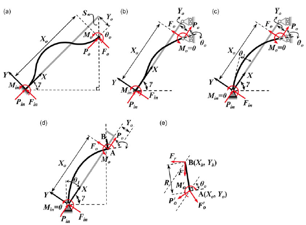
The modeling of the three basic CFM configurations, along with the improved configuration, is presented in this appendix. The corresponding force analysis is illustrated in Figure A2. To better represent the loading conditions encountered in practical design, the coordinate system is rotated by an angle $\gamma$
relative to Figure A1, while the beam axis remains aligned with the X-axis for modeling purposes. The boundary conditions and force equilibrium equations for each configuration are summarized as follows:
$\gamma$
relative to Figure A1, while the beam axis remains aligned with the X-axis for modeling purposes. The boundary conditions and force equilibrium equations for each configuration are summarized as follows:
(1) For the FF-type CFM shown in Figure A2(a), the prescribed boundary conditions are:
 \begin{align}X_{o}&=L-S\cdot sin\gamma \nonumber \\[2pt] Y_{o}&=-S\cdot cos\gamma \nonumber \\[2pt] \theta _{o}&=0\end{align}
(2) For the FP-type CFM shown in Figure A2(b), the prescribed boundary conditions are:
 \begin{align}X_{o}&=L-S\cdot sin\gamma \nonumber \\[2pt] Y_{o}&=-S\cdot cos\gamma \nonumber \\[2pt] m_{o}&=0\end{align}
(3) For the PP-type CFM shown in Figure A2(c), the prescribed boundary conditions are:
 \begin{align}X_{o}&=L-S\cdot sin\gamma \nonumber \\[2pt] Y_{o}&=-S\cdot cos\gamma \nonumber \\[2pt]0&=P_{o}Y_{o}-F_{o}X_{o}\end{align}
(4) For the improved PP-type CFM shown in Figures A2(d) and A2(e), the boundary conditions differ from those of the standard PP configuration. Specifically, the prescribed condition at point A is replaced by a prescribed condition at point B, expressed as
 \begin{align}X_{b}&=L-S\cdot sin\gamma \nonumber \\[2pt] Y_{b}&=-S\cdot cos\gamma\end{align}

Figure A1. Kinetostatic model of CFM: discretization of the i-th compliant beam.

Figure A2. Force analysis of buckling-based CFMs: (a) FF-type; (b) FP-type; (c) PP-type; (d) and (e) improved PP-type.
As illustrated in Figure A2(d), the force equilibrium equations for beam segment OA can be established by taking moments about point O:
 \begin{equation}0=P_{\! o}Y_{o}-F_{\! o}X_{o}-M_{o}\end{equation}
As shown in Figure A2(e), for the rigid segment AB fixed at point A and perpendicular to beam OA, the following equilibrium equations are obtained:
 \begin{equation}0={P_{\! o}^{'}}R\cdot cos\theta _{o}-{{F}_{\! o}^{'}}R\cdot sin\theta _{o}+{{M}_{\! o}^{'}}\end{equation}
At point A, the following conditions must also be satisfied:
 \begin{align}{{P}_{\! o}^{'}}=-{{P}_{\! o}}\nonumber\\ {{F}_{\! o}^{'}}=-{{F}_{\! o}}\nonumber\\ {{M}_{\! o}^{'}}=-{{M}_{\! o}}\end{align}
Since segment AB is rigid, the coordinates of point A can be determined from the coordinates of point B and the end rotation angle θ o :
 \begin{align}X_{o}=X_{b}-R\cdot sin\theta _{o} \nonumber \\[2pt] Y_{o}=Y_{o}-R\cdot cos\theta _{o}\end{align}
In addition to the above boundary conditions or supplementary equilibrium equations specific to each configuration, the following set of common governing equations applies to all four structures. The static equilibrium equation between the beam’s endpoint A and the first segment element can be expressed as
 \begin{equation}\left[\begin{array}{c} p_{o}\\ f_{o}\\ m_{o} \end{array}\right]=\left[\begin{array}{c} p_{1}\\ f_{1}\\ m_{N} \end{array}\right]\end{equation}
The static equilibrium relationship between each beam segment is
 \begin{equation}\left[\begin{array}{c@{\quad}c@{\quad}c} cos\theta _{i} & sin\theta _{i} & 0\\[2pt] -sin\theta _{i} & cos\theta _{i} & 0\\[2pt] \left(1+\lambda _{i}\right) & -\delta _{i} & 1 \end{array}\right]\left[\begin{array}{c} f_{i}\\[2pt] p_{i}\\[2pt] m_{i} \end{array}\right]=\left[\begin{array}{c} f_{1}\\[2pt] p_{1}\\[2pt] m_{i-1} \end{array}\right]\end{equation}
where θ i represents the rotation angle of the coordinate system O i X i Y i of the i-th segment relative to the global coordinate system. The rotation angles of the other segments can be expressed as
 \begin{equation}\theta _{i}=\sum _{k=1}^{i-1}\alpha _{k}+\theta _{1},\,i=2,3,\ldots ,N\end{equation}
The BCM equation is given by
 \begin{align}\left[\begin{array}{c} \begin{array}{c} f_{i} \end{array}\\ m_{i} \end{array}\right]=\left[\begin{array}{c@{\quad}c} 12 & -6\\ -6 & 4 \end{array}\right]\left[\begin{array}{c} \begin{array}{c} \begin{array}{c} \delta _{i} \end{array} \end{array}\\ \alpha _{i} \end{array}\right]+\frac{p_{i}}{30}\left[\begin{array}{c@{\quad}c} 36 & -3\\ -3 & 4 \end{array}\right]\left[\begin{array}{c} \begin{array}{c} \begin{array}{c} \delta _{i} \end{array} \end{array}\\ \alpha _{i} \end{array}\right]+\frac{p_{i}^{2}}{6300}\left[\begin{array}{c@{\quad}c} -9 & 4.5\\ 4.5 & -11 \end{array}\right]\left[\begin{array}{c} \begin{array}{c} \begin{array}{c} \delta _{i} \end{array} \end{array}\\ \alpha _{i} \end{array}\right]\nonumber\\[3pt] \lambda _{i}=\frac{t^{2}p_{i}}{12}-\frac{1}{60}\left[\begin{array}{c@{\quad}c} \delta _{i} & \alpha _{i} \end{array}\right]\left[\begin{array}{c@{\quad}c} 36 & -3\\ -3 & 4 \end{array}\right]\left[\begin{array}{c} \begin{array}{c} \begin{array}{c} \delta _{i} \end{array} \end{array}\\ \alpha _{i} \end{array}\right]-\frac{p_{i}}{6300}\left[\begin{array}{c@{\quad}c} \delta _{i} & \alpha _{i} \end{array}\right]\left[\begin{array}{c@{\quad}c} -9 & 4.5\\ 4.5 & -11 \end{array}\right]\left[\begin{array}{c} \begin{array}{c} \begin{array}{c} \delta _{i} \end{array} \end{array}\\ \alpha _{i} \end{array}\right]\end{align}
The geometric relationships between segments are expressed as
 \begin{align}&\sum _{i=1}^{N}\left[\left(1+\lambda _{i}\right)cos\,\theta _{i}-\delta _{i} \, sin\,\theta _{i}\right]=x_{o}\nonumber\\[-3pt] &\sum _{i=1}^{N}\left[\left(1+\lambda _{i}\right)sin\,\theta _{i}+\delta _{i} \, cos\,\theta _{i}\right]=y_{o}\nonumber\\[-3pt] &\quad\quad\quad\sum _{i=1}^{N}\alpha _{i}=\theta _{o}\end{align}
Under a known displacement S, all unknown variables of the four configurations can be determined by combining their specific equations with Eqs. A(10)–A(14).Additionally, the strain energy of the entire structure can be expressed as
 \begin{equation}V_{T}=\sum _{i=1}^{N}\frac{v_{i}\cdot EI}{L_{i}}\end{equation}
where ν i represents the nondimensionalized expression of the strain energy for each element:
 \begin{equation}v_{i}=\frac{t^{2}p_{i}^{2}}{24}+\left[\begin{array}{c@{\quad}c} \delta _{i} & \alpha _{i} \end{array}\right]\left[\begin{array}{c@{\quad}c} 6 & -3\\ -3 & 2 \end{array}\right]\left[\begin{array}{c} \begin{array}{c} \begin{array}{c} \delta _{i} \end{array} \end{array}\\ \alpha _{i} \end{array}\right] -\frac{p_{i}^{2}}{12600}\left[\begin{array}{c@{\quad}c} \delta _{i} & \alpha _{i} \end{array}\right]\left[\begin{array}{c@{\quad}c} -9 & 4.5\\ 4.5 & -11 \end{array}\right]\left[\begin{array}{c} \begin{array}{c} \begin{array}{c} \delta _{i} \end{array} \end{array}\\ \alpha _{i} \end{array}\right]\end{equation}
Appendix B. Reference values of critical slenderness ratios for materials used in compliant mechanisms
Table B1. Four materials in compliant mechanism design.

Appendix C. The influence of parameter R on CFMs
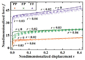
To investigate the specific influence of parameter r on the force–displacement relationships of the structure, a representative set of design parameters is selected within the design space ( $\gamma$
= 88°, t = 0.005). The effect of varying r from 0 to 0.04 is analyzed, as shown in Figure C1. The results indicate that a smaller value of r leads to a more abrupt transition from the force rise phase to constant force phase. However, the overall shape of the force–displacement curve is not significantly altered by r, with all configurations converging toward a similar trend as displacement increases.
$\gamma$
= 88°, t = 0.005). The effect of varying r from 0 to 0.04 is analyzed, as shown in Figure C1. The results indicate that a smaller value of r leads to a more abrupt transition from the force rise phase to constant force phase. However, the overall shape of the force–displacement curve is not significantly altered by r, with all configurations converging toward a similar trend as displacement increases.

Figure C1. The influence of parameter r on the force-displacement characteristics of the CFM.
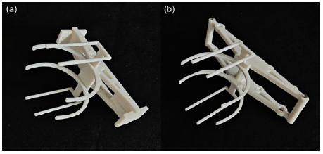
Appendix D. Details of gripper geometry used in experiments

Figure D1. Grippers used in the two catapult prototypes: (a) linear-spring catapult, (b) CFM catapult.