





1. Introduction
The development of microfluidic devices has lead to novel technological and biomedical applications by making possible rapid sorting, mixing and focusing of various small biological or synthetic constituents (Giddings Reference Giddings1993; Stone, Stroock & Ajdari Reference Stone, Stroock and Ajdari2004; Whitesides Reference Whitesides2006; Shields, Reyes & López Reference Shields IV, Reyes and López2015). The future design of ‘lab-on-a-chip’ devices, which, due to their small size, can be used routinely in different settings, could be important e.g. in the analysis of single cells (Stott et al. Reference Stott2010; Hosic, Murthy & Koppes Reference Hosic, Murthy and Koppes2016; Qasaimeh et al. Reference Qasaimeh, Wu, Bose, Menachery, Talluri, Gonzalez, Fulciniti, Karp, Prabhala and Karnik2017; Farahinia, Zhang & Badea Reference Farahinia, Zhang and Badea2021), thereby allowing for rapid disease detection or for advancing the fundamental understanding of biological processes.
Microfluidic approaches have been utilized to guide and control transport processes for several objectives. Examples range from the separation of the components of blood, such as red or white blood cells (Huang et al. Reference Huang, Cox, Austin and Sturm2004; Davis et al. Reference Davis, Inglis, Morton, Lawrence, Huang, Chou, Sturm and Austin2006; McGrath, Jimenez & Bridle Reference McGrath, Jimenez and Bridle2014), to the focusing and detection of biological cells (Qasaimeh et al. Reference Qasaimeh, Wu, Bose, Menachery, Talluri, Gonzalez, Fulciniti, Karp, Prabhala and Karnik2017; Farahinia et al. Reference Farahinia, Zhang and Badea2021), to the mixing of particulate suspensions (Stroock et al. Reference Stroock, Dertinger, Whitesides and Ajdari2002a,Reference Stroock, Dertinger, Ajdari, Mezić, Stone and Whitesidesb; Stroock & McGraw Reference Stroock and McGraw2004). The underlying methods rely on different physical mechanisms, such as ‘active’ concepts, which use externally applied forces and filters (Giddings Reference Giddings1993; Stone et al. Reference Stone, Stroock and Ajdari2004; Shields et al. Reference Shields IV, Reyes and López2015) or ‘passive’ concepts, which exploit hydrodynamic effects due to fluid inertia (Segré & Silberberg Reference Segré and Silberberg1961; Di Carlo et al. Reference Di Carlo, Irimia, Tompkins and Toner2007; Humphry et al. Reference Humphry, Kulkarni, Weitz, Morris and Stone2010), pillar arrays in channels (Huang et al. Reference Huang, Cox, Austin and Sturm2004; Davis et al. Reference Davis, Inglis, Morton, Lawrence, Huang, Chou, Sturm and Austin2006; McGrath et al. Reference McGrath, Jimenez and Bridle2014), or patterned microfluidic walls (Stroock et al. Reference Stroock, Dertinger, Ajdari, Mezić, Stone and Whitesides2002b; Choi & Park Reference Choi and Park2007; Hsu et al. Reference Hsu, Di Carlo, Chen, Irimia and Toner2008; Choi et al. Reference Choi, Ku, Song, Choi and Park2011; Asmolov et al. Reference Asmolov, Dubov, Nizkaya, Kuehne and Vinogradova2015; Qasaimeh et al. Reference Qasaimeh, Wu, Bose, Menachery, Talluri, Gonzalez, Fulciniti, Karp, Prabhala and Karnik2017).
Several passive approaches utilize surface topography, relying on the careful design and synthesis of surface structures, mostly at the micron scale. Corrugations oriented obliquely to the axial flow direction or v-shaped herringbone structures were proposed originally for the mixing of laminar streams (Stroock et al. Reference Stroock, Dertinger, Whitesides and Ajdari2002a,Reference Stroock, Dertinger, Ajdari, Mezić, Stone and Whitesidesb; Stroock & McGraw Reference Stroock and McGraw2004). In addition to mixing, passive approaches have been used to separate or detect particles. For example, microfluidic channels with oblique corrugations on one wall have been applied widely to separate colloidal particles (Choi & Park Reference Choi and Park2007; Hsu et al. Reference Hsu, Di Carlo, Chen, Irimia and Toner2008; Choi et al. Reference Choi, Ku, Song, Choi and Park2011) and for the detection of plasma (Qasaimeh et al. Reference Qasaimeh, Wu, Bose, Menachery, Talluri, Gonzalez, Fulciniti, Karp, Prabhala and Karnik2017) or circulating tumour cells (Stott et al. Reference Stott2010). The parallel oblique corrugations on the top or bottom wall generate a transverse pressure gradient, and due to the lateral confinement of the channel, helical streamlines result, where the pitch of the helix spans several corrugations (Stroock et al. Reference Stroock, Dertinger, Whitesides and Ajdari2002a,Reference Stroock, Dertinger, Ajdari, Mezić, Stone and Whitesidesb; Stroock & McGraw Reference Stroock and McGraw2004). The recirculating flows generated by the corrugations, which will be in opposite lateral directions at the corrugated and flat surfaces, transport particles to each lateral wall depending on the particle's position along the channel height, which depends, for example on the particle's size or density, and can be controlled using inertial focusing (Segré & Silberberg Reference Segré and Silberberg1961; Di Carlo et al. Reference Di Carlo, Irimia, Tompkins and Toner2007). Therefore, particles with different properties can be transported to opposite lateral walls and sorted according to the property of interest. Similarly, v-shaped, or herringbone, corrugations create counter-rotating vortices in the microchannel. These flows bring particles to their equilibrium configuration between adjacent vortices either near the herringbone surface or near the planar wall, depending on their density, to separate particles into different streams for sorting or detection (Hsu et al. Reference Hsu, Di Carlo, Chen, Irimia and Toner2008).
The aforementioned studies focused on the recirculating flows, generated by surface topography, at the scale of the channel size. The effect of surface structure on the flow and particle motion near the surface, at the scale of individual corrugations, remains relatively unexplored. Recent insights for the non-trivial trajectories come from our work on particle sedimentation near corrugated surfaces (Chase, Kurzthaler & Stone Reference Chase, Kurzthaler and Stone2022), where we quantified, experimentally and theoretically, the impact of corrugation shape and particle size on the transport behaviour without background flow and due only to the disturbance flow generated by the interaction of the particle and surface structure. In contrast to results observed in microfluidic channels, where particles are separated by size due to differences in their equilibrium positions along the channel height, it was shown that the magnitude of the lateral displacement for particles of different sizes depends not only on their distance to the corrugated wall, but on non-trivial relationships between the particle size and corrugation wavelength.
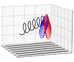
Here, we complement these findings by studying pressure-driven flow between a corrugated surface and a parallel flat wall. Using a perturbation ansatz for the amplitude of the surface structure, we calculate the pressure field induced by the surface pattern and derive analytical expressions for the three-dimensional flow fields up to second order in the surface roughness. Based on these results, we determine the motion of tracer particles near the corrugated wall. While the large-scale helicoidal flows in corrugated microchannels, generated by the combined effect of the corrugations and the lateral confining walls, have diameter equal to that of the channel dimension and a pitch of several wavelengths (Stroock et al. Reference Stroock, Dertinger, Whitesides and Ajdari2002a), our results reveal that tracer particles also follow three-dimensional helical trajectories, independent of the lateral confining walls, which have a pitch of one wavelength and a diameter that depends on the distance to the corrugated surface and the corrugation wavelength. Projected to two dimensions, the trajectories of tracer particles resemble the oscillatory near-surface motion observed in several experiments (Choi & Park Reference Choi and Park2007; Hsu et al. Reference Hsu, Di Carlo, Chen, Irimia and Toner2008; Choi et al. Reference Choi, Ku, Song, Choi and Park2011; Qasaimeh et al. Reference Qasaimeh, Wu, Bose, Menachery, Talluri, Gonzalez, Fulciniti, Karp, Prabhala and Karnik2017). The oscillatory pattern is characterized by near-surface particle motion along the corrugations while moving above grooves and across the corrugations while moving over ridges. Moreover, our results demonstrate that near-surface particles exhibit an overall drift along the surface corrugations, leading to a skewed helical trajectory. We quantify the overall displacement as a function of surface wavelength and particle position along the channel height, showing that the lateral drift can be achieved independent of the recirculating flows generated in closed channels.
Our paper is structured as follows. In § 2, we outline a hydrodynamic model for the pressure-driven flow between a flat wall and a parallel rough wall. In § 3, we describe our experimental method for measuring the flow field in a corrugated microchannel using particle image velocimetry. To our knowledge, this is the first experimental measurement of velocity fields in corrugated microchannels. We also outline our method for three-dimensional single-particle tracking in the corrugated channels. In § 4, we provide experimental and theoretical results for the roughness-induced pressure and flow fields and compare them qualitatively and quantitatively. Furthermore, we find good agreement between our experimentally measured mean velocities and the theory from Stroock et al. (Reference Stroock, Dertinger, Whitesides and Ajdari2002a) for flows generated in corrugated microchannels with confining lateral walls. Most importantly, our results are complemented by theoretical and experimental measurements of three-dimensional helical particle trajectories. Finally, we investigate the effect of the ratio of corrugation wavelength to channel height for varying positions along the channel height on the lateral drift of tracer particles in the flow.
2. Hydrodynamic model
We consider three-dimensional, low-Reynolds-number, pressure-driven flow between two plates, where the lower surface has a given shape  $z = \epsilon L\,H(x,y)$, with shape function $H(x,y)$, as indicated in figure 1. Here, $L$ denotes the distance between the upper surface and the reference surface $S_0$, and we denote by $\epsilon$ a dimensionless roughness parameter. The velocity and pressure fields, $\boldsymbol {u}(x,y,z)$ and $p(x,y,z)$, respectively, obey the Stokes and continuity equations,
 \begin{equation} \mu\,\nabla^2\boldsymbol{u}=\boldsymbol{\nabla} p \quad \text{and} \quad \boldsymbol{\nabla} \boldsymbol{\cdot}\boldsymbol{u}=0, \end{equation}
where  $\mu$ denotes the fluid viscosity. We have no-slip boundary conditions on the lower and upper surfaces: $\boldsymbol {u}(x,y,z=\epsilon L\,H(x,y))=\boldsymbol {0}$ and $\boldsymbol {u}(x,y,z=L)=\boldsymbol {0}$. Subsequently, we consider small surface corrugations, corresponding to $\epsilon \ll 1$, and expand the flow field up to third order in the small parameter $\epsilon$:
 \begin{equation} \boldsymbol{u}=\boldsymbol{u}^{(0)}+\epsilon \boldsymbol{u}^{(1)}+ \epsilon^2\boldsymbol{u}^{(2)}+ O(\epsilon^3). \end{equation}
Sketch of pressure-driven flow between the lower corrugated surface  $S_w$ and the upper planar wall (side view). Here, $L$ denotes the distance between the upper surface and a reference surface $S_0$ at $z=0$, $H(x,y)$ is the shape function, and $\epsilon$ is the surface roughness.

An average pressure gradient is applied along the direction of the flow,  $\langle \mathrm {d} p/\mathrm {d}x\rangle =-G$, hence we rescale by
 \begin{equation}
\boldsymbol{u}=
\frac{GL^2}{2\mu}\,\boldsymbol{U},\quad p = GL P,\quad
x = LX,\quad y = LY,\quad z=LZ.
\end{equation}
\begin{equation}
\boldsymbol{u}=
\frac{GL^2}{2\mu}\,\boldsymbol{U},\quad p = GL P,\quad
x = LX,\quad y = LY,\quad z=LZ.
\end{equation}By using the method of domain perturbation (Kamrin, Bazant & Stone Reference Kamrin, Bazant and Stone2010; Kurzthaler et al. Reference Kurzthaler, Zhu, Pahlavan and Stone2020), we obtain the boundary conditions for the components of the expansion:
 $$\begin{gather} \boldsymbol{U}^{(0)}= \boldsymbol{0},\quad \boldsymbol{U}^{(1)}=-H(X,Y)\left.\frac{\partial\boldsymbol{U}^{(0)}}{\partial Z}\right|_{Z=0}, \end{gather}$$
 $$\begin{gather}\boldsymbol{U}^{(2)}=-H(X,Y)\left.\frac{\partial\boldsymbol{U}^{(1)}}{\partial Z}\right|_{Z=0} -\frac{1}{2}\,H(X,Y)^2 \left.\frac{\partial^2\boldsymbol{U}^{(0)}}{\partial Z^2}\right|_{Z=0} \quad \text{on } Z=0, \end{gather}$$
 $$\begin{gather}\boldsymbol{U}^{(0)}=\boldsymbol{0},\quad \boldsymbol{U}^{(1)}=\boldsymbol{0}, \quad \boldsymbol{U}^{(2)}=\boldsymbol{0} \quad \text{on } Z=1. \end{gather}$$
We note that the zeroth-order flow field is pressure-driven flow between parallel plates,  $\boldsymbol {U}^{(0)}=Z(1-Z)\boldsymbol {e}_X$, and the pressure is $P^{(0)}=-X \boldsymbol {e}_X$. Thus the boundary conditions (2.4a–2.4b) on $Z=0$ simplify to $\boldsymbol {U}^{(1)}(X,Y,Z=0) = -H(X,Y)\,\boldsymbol {e}_X$ and $\boldsymbol {U}^{(2)}(X,Y,Z=0) =-H(X,Y)\,\partial \boldsymbol {U}^{(1)}/\partial Z|_{Z=0}+H(X,Y)^2\,\boldsymbol {e}_X$.
Generally, one can calculate the first-order perturbation  $\boldsymbol {U}^{(1)}$ by applying a Fourier transform to the $X$- and $Y$-components,
 \begin{equation} \tilde{\boldsymbol{U}}(K_X,K_Y,Z) = \frac{1}{2{\rm \pi}}\int_{\mathbb{R}^2} \exp({-\mathrm{i} (K_XX+K_YY)})\,\boldsymbol{U}(X,Y,Z)\,\mathrm{d}X \,\mathrm{d}Y; \end{equation}
the inverse transform is  $\boldsymbol {U}(X,Y,Z) = (2{\rm \pi} )^{-1}\int _{\mathbb {R}^2} \exp ({\mathrm {i} (K_XX+K_YY)})\, \tilde {\boldsymbol {U}}(K_X, K_Y,Z) \,\mathrm {d} K_X$ $\mathrm {d} K_Y$. The Stokes and continuity equations (2.1a,b) then simplify to
 $$\begin{gather} \left(\frac{\textrm{d}^2}{\textrm{d} Z^2}-K^2\right)\tilde{\boldsymbol{U}}^{(1)}= \left(\mathrm{i} \boldsymbol{K}+ \boldsymbol{e}_Z\,\frac{\textrm{d}}{\textrm{d} Z}\right)\tilde{P}^{(1)}, \end{gather}$$
 $$\begin{gather}\mathrm{i} \boldsymbol{K}\boldsymbol{\cdot}\tilde{\boldsymbol{U}}^{(1)}+ \frac{\textrm{d} \tilde{W}^{(1)}}{\textrm{d} Z}=0, \end{gather}$$
where we have used  $\tilde {\boldsymbol {U}}^{(1)}=[\tilde {U}^{(1)},\tilde {V}^{(1)}, \tilde {W}^{(1)}]^{\rm T}$, $\boldsymbol {K}=[K_X, K_Y,0]^{\rm T}$ and $K=|\boldsymbol {K}|$. Rearranging (2.6a)–(2.6b) provides an equation for the pressure field,
 \begin{equation} \left(\frac{\textrm{d}^2}{\textrm{d} Z^2}-K^2\right)\tilde{P}^{(1)}=0, \end{equation}
which can be solved by  $\tilde {P}^{(1)}=p_0(K)\exp (-KZ)+p_1(K)\exp (KZ)$.
Using this form as input for (2.6a)–(2.6b), we can calculate the velocity field  $\boldsymbol {U}^{(1)}$ and determine the coefficients $p_0$ and $p_1$ by enforcing the boundary conditions (2.4a) and (2.4c), which depend on the surface shape $H(X,Y)$. Knowledge of the first-order flow field $\boldsymbol {U}^{(1)}$ then allows us to compute iteratively the second-order flow field $\boldsymbol {U}^{(2)}$ with boundary conditions in (2.4b)–(2.4c). The velocity fields obtained via the domain-perturbation approach have been validated with numerical simulations of the full hydrodynamic flows (assuming a shear flow scenario) by Roggeveen, Stone & Kurzthaler (Reference Roggeveen, Stone and Kurzthaler2023). In particular, the error of the perturbative approach remained small for small surface roughness and moderate for large wavelengths $\lambda /L\gtrsim 2$.
It is worth emphasizing that the theory is, in principle, valid for arbitrary surface shapes. However, analytical progress is limited by whether the surface shape function  $H(X,Y)$ and powers of it (e.g. $H(X,Y)^2$ is required for the second-order flow field) have an analytically tractable Fourier transform. Furthermore, one may need to perform a numerical backtransform of the pressure and flow fields to real space. For cosine and sine functions, the calculations can be done analytically. Consequently, for every shape function that can be expanded in terms of a Fourier series (i.e. periodic, piecewise continuous, and integrable over the period), our approach allows calculation (semi-)analytically of the flow fields.
At this point, we want to mention that the stream function for two-dimensional shear flow near a periodic surface has been addressed recently (Assoudi, Lamzoud & Chaoui Reference Assoudi, Lamzoud and Chaoui2018). Also, analytical work on the three-dimensional streamlines over sinusoidal surface grooves, tilted with respect to the principal flow direction, has provided a prediction for the helicity of the flow (Stroock et al. Reference Stroock, Dertinger, Whitesides and Ajdari2002a). The same authors later calculated the flow over herringbone structures in a channel of finite width in terms of a Fourier expansion by approximating the surface grooves with an effective slip velocity (Stroock & McGraw Reference Stroock and McGraw2004). The focus of the latter study, however, was on the impact of the corrugated surfaces on the mixing of particulate suspensions.
3. Experimental methods
We fabricate two channels, both with corrugations of wavelength  $\lambda$ on the top wall, but with different channel heights $L$, therefore varying the ratio of $\lambda /L$. We 3-D print moulds of the negative of each channel (Formlabs Form 2), and cast a clear channel from polydimethylsiloxane (PDMS). We punch inlet and outlet holes, and bond the PDMS channel to a glass slide (figure 2a). One channel has height $L=320\,\,\mathrm {\mu }{\rm m}$ and surface amplitude $\epsilon L =30\,\,\mathrm {\mu }{\rm m}$. The second channel has height $L=615\,\,\mathrm {\mu }{\rm m}$ and surface amplitude $\epsilon L =60\,\,\mathrm {\mu }{\rm m}$. The wavelength of the surface corrugations for both channels is $\lambda =600\,\,\mathrm {\mu }{\rm m}$, and the aspect ratio (width to height) of both channels is 10. The channel height and corrugation wavelength and amplitude were measured by filling the channel with a fluorescent dye and taking $xz$ images using a confocal microscope (Leica) (figure 2b).
Experiments. (a) The channel used in the experimental system is cast polydimethylsiloxane (PDMS) with corrugations on the upper wall. (b) A cross-sectional view of the channel visualized with fluorescent dye. Here, the wavelength is  $\lambda =600\,\,\mathrm {\mu }{\rm m}$, the height is $L=320\,\,\mathrm {\mu }{\rm m}$, and the amplitude is $\epsilon L=30\,\,\mathrm {\mu }{\rm m}$. (c) Flow field visualization of pressure-driven flow in the corrugated channel from a time stack of 200 experimental images taken at frame rate 7.4 fps with $1\,\,\mathrm {\mu }{\rm m}$ diameter fluorescent particles. (d) Visualization of the trajectory of a $5\,\,\mathrm {\mu }{\rm m}$ diameter particle in pressure-driven flow in the corrugated channel.

To measure the flow field in the channel, we use a syringe pump, with prescribed flow rates  $2.5$ and $10\,\mathrm {\mu }\textrm {l}\,\textrm {min}^{-1}$, respectively, for the $L=320$ and $615\,\,\mathrm {\mu }{\rm m}$ channels, to flow a suspension of neutrally buoyant fluorescent $1\,\,\mathrm {\mu }{\rm m}$ diameter tracer particles through the channel. We use a confocal microscope (Leica) to image a $916\,\,\mathrm {\mu }{\rm m} \times 916\,\,\mathrm {\mu }{\rm m}$ section in $xy$ at frame rate $7.4\,\textrm {fps}$ and capture 200 frames. Using PIV Lab (Stamhuis & Thielicke Reference Stamhuis and Thielicke2014; Thielicke & Sonntag Reference Thielicke and Sonntag2021) in MATLAB (MathWorks), we perform particle image velocimetry of the steady flow field to measure the axial and transverse components of the velocity. We image at 40 different $z$-positions along the channel height. A stack of 200 time series images at $z=120\,\,\mathrm {\mu }{\rm m}$ is shown in figure 2(c), where the oscillations of the streamlines are visible as bright streaks.
In addition to measuring the flow field in the  $xy$-plane, we can measure the three-dimensional trajectories of individual tracer particles. For the same channels, we flow a dilute suspension of neutrally buoyant fluorescent tracer particles with diameter $5\,\,\mathrm {\mu }{\rm m}$ through the channel at a constant flow rate using a syringe pump. We take $xyzt$ images using a confocal microscope (Leica). The $xy$ image is $916\,\,\mathrm {\mu }{\rm m}$ by $230\,\,\mathrm {\mu }{\rm m}$, and we image 27 sections in $z$ with step size $2.365\,\,\mathrm {\mu }{\rm m}$ at frame rate 18 fps, acquiring the $xyz$ volume in 1.5 seconds. For every time step, we find the $(x, y)$ location of the particle using the circle detection algorithm in MATLAB (Mathworks). We determine the $z$-position of the particle at each time step by first cropping the image around the particle location and calculating $G(z) = \sum I(x,y)$, where $I(x,y)$ is the image intensity, for each image in the $z$-stack. The image with $\max (G)$ is determined to be the $z$-position of the particle. We iterate this process for each time step to find the particle trajectory $(x(t),y(t),z(t))$. A sample trajectory, projected to the $xy$-plane, is shown as the superposition of the frames of the determined best $z$-position for each time step in figure 2(d).
Our experiments have Stokes number  $S_{tk}\approx 10^{-9}$, where the Stokes number is defined by $S_{tk} = {\rho _p d_p^2 U}/{18\mu D}$. Here, $\rho _p$ is the particle density, $d_p$ is the particle diameter, $U$ is the characteristic fluid velocity, $\mu$ is the fluid viscosity, and $D$ is the hydraulic diameter of the channel.
4. Results and discussion
While the theory presented in § 2 is valid for arbitrary surface shapes, here we study the aspect of parallel corrugations, reminiscent of the pattern used widely in microfluidic devices (Stroock et al. Reference Stroock, Dertinger, Ajdari, Mezić, Stone and Whitesides2002b; Choi & Park Reference Choi and Park2007; Hsu et al. Reference Hsu, Di Carlo, Chen, Irimia and Toner2008; Choi et al. Reference Choi, Ku, Song, Choi and Park2011; Qasaimeh et al. Reference Qasaimeh, Wu, Bose, Menachery, Talluri, Gonzalez, Fulciniti, Karp, Prabhala and Karnik2017). We consider a surface shape  $H(X,Y)=\cos (K_0 (X+Y))$ characterized by the wavenumber $k_0=K_0/L$, corresponding to a wavelength $\lambda = 2{\rm \pi} /k_0$. We note that the surface corrugations are at angle ${\rm \pi} /4$ to the direction of the applied pressure gradient (see figure 3a). In what follows, we refer to fluid transport along corrugations when a fluid particle moves on a path in the positive $X$-direction but with displacement in the negative $Y$-direction, and across corrugations when the flow path is instead in the positive $Y$-direction.
Surface structure and roughness-induced pressure. (a) Contour plot of the surface structure  $H(X,Y)$. The grey shaded areas indicate the height profile of the underlying surface, where dark areas correspond to grooves, and white areas to ridges, respectively. The arrow indicates the direction of the applied pressure gradient. (b) Contour plot of the roughness-induced components of the pressure field $P-P^{(0)} = \epsilon P^{(1)}+\epsilon ^2 P^{(2)}$ at the centre of the channel $Z=0.2$. Here, the black dashed lines correspond to the maxima of the surface structure. (c) Roughness-induced pressure along $X$ at $Y= 0$ for varying $Z$. The black dashed line corresponds to $H(X,Y)$. The wavelength in (b,c) is $\lambda /L=2$. The applied pressure gradient is in the $X$-direction.

To compute the pressure and flow fields, we follow the general approach outlined in § 2. Therefore, we use the Fourier transform of the surface shape  $\tilde {H}(K_X, K_Y)={\rm \pi} [\delta (K_0+K_X)\,\delta (K_0+K_Y)+\delta (K_0-K_X)\,\delta (K_0-K_Y)]$, where $\delta (\cdot )$ denotes the delta function, as input to calculate the pressure $\tilde {P}^{(1)}$ and the velocity field $\tilde {\boldsymbol {U}}^{(1)}$ in Fourier space and transform back to real space analytically. We repeat this for the second-order flow field $\boldsymbol {U}^{(2)}$, where the Fourier backtransform is still doable but becomes tedious. An alternative way to compute the flow fields, which relies on the sinusoidal form of the surface shape, is outlined by Roggeveen et al. (Reference Roggeveen, Stone and Kurzthaler2023).
4.1. Roughness-induced pressure fields
We find that the surface corrugations lead to the generation of a pressure field  $P$ that varies with position. In particular, the zeroth-order pressure field is $P^{(0)}=-X$, and the first-order pressure field evaluates to
 \begin{align} P^{(1)} (X,Y,Z) &=\sin(K_0(X+Y))\,\frac{K_0\exp({-K_0\sqrt{2}(2+Z)})}{1+4K_0^2-\cosh(2\sqrt{2}K_0)} \nonumber\\ &\quad \times [\exp({2 \sqrt{2} K_0 Z})+\exp({4 \sqrt{2} K_0})+(2 \sqrt{2} K_0-1) \nonumber\\ &\quad \times \exp({2 \sqrt{2} K_0(Z+1)})-\exp({2 \sqrt{2} K_0})\,(2 \sqrt{2} K_0+1)]. \end{align}
Higher-order terms are lengthy and not presented here. For a corrugated surface  $H(X,Y)=\cos {(K_0(X+Y))}$ (see figure 3a), the roughness-induced contributions to the pressure field at $Z=0.2$ are shown in figure 3(b). Plotting the roughness-induced contributions to $P$ along $X$ at $Y=0$ for varying $Z$-positions (figure 3c), we see that the pressure builds up in front of the surface ridges and decreases in front of the surface grooves, where the surface shape is depicted by the black dashed line.
In particular, the first-order contribution to the pressure, which can be abbreviated by  $P^{(1)}=\sin (K_0(X+Y))\,\bar {P}^{(1)}(Z)$ (see (4.1)), has its extrema at the inflection points of the surface, i.e. at points of vanishing curvature, $\cos (K_0(X+Y))=0$. The extrema are at $X+Y=(2n+1){\rm \pi} /(2K_0)= (2n+1) \lambda /(4L)$ for $n\in \mathbb {Z}$, with minima at $X+Y=(4n+1)\lambda /(4L)$ and maxima at $X+Y=(4n-1)\lambda /(4L)$. The inflection points are modified by the second-order contribution $P^{(2)}$.
We find that the magnitude of the roughness-induced contributions to the pressure decrease as  $Z$ increases, moving towards the flat upper wall (figure 3). Finally, we note that the pressure field generated by the corrugated surface is anisotropic relative to the direction of the applied pressure gradient, along $X$ (figure 3b), and can therefore induce, in addition to flows along the $Z$-direction, transverse flows (in the $XY$-plane).
4.2. Roughness-induced flow fields
The streamlines along the channel ( $XZ$-plane), shown in figure 4(a), display oscillations over the surface corrugations, which vanish near the flat upper wall. Furthermore, we find a non-vanishing lateral velocity field in the $YZ$-plane (figure 4b), which is generated solely by the corrugated surface. In particular, the flow moves in opposite $Y$-directions over surface ridges compared to grooves. This response leads to flow patterns, which alternate their direction depending on the underlying surface structure.
Theoretical and experimental velocity fields. (a,b) Streamlines of the theoretical velocity field in (a) the  $XZ$-plane, $[U^{(0)}+\epsilon U^{(1)}+\epsilon ^2U^{(2)}, W^{(0)}+\epsilon W^{(1)}+\epsilon ^2W^{(2)}]^{\rm T}$, and (b) the $YZ$-plane, $[V^{(0)}+\epsilon V^{(1)}+\epsilon ^2V^{(2)}, W^{(0)}+\epsilon W^{(1)}+\epsilon ^2W^{(2)}]^{\rm T}$. The grey areas indicate the surface shape from the side. (c,d) Streamlines of the theoretical velocity field in the $XY$-plane, $[U^{(0)}+\epsilon U^{(1)}+\epsilon ^2U^{(2)}, V^{(0)}+\epsilon V^{(1)}+\epsilon ^2V^{(2)}]^{\rm T}$, at (c) $Z=0.20$ and (d) $Z=0.35$. The grey shaded areas indicate the height profile of the underlying surface, where dark areas correspond to grooves and white areas to ridges, respectively (see colour map in figure 3a). (e,f) Streamlines of the experimental velocity field in the $XY$-plane at (e) $Z=0.20$ and (f) $Z=0.35$. In all plots, the wavelength is $\lambda /L = 1.87$ and the surface roughness is $\epsilon = 0.094$. Furthermore, the colour map corresponds to the magnitude of the velocity in a particular plane. Note that for the experimental velocities, the magnitude includes only the $X$- and $Y$-components of the velocity, since the $Z$-component is not measured.

The streamlines ( $XY$-plane) are oscillatory in the transverse ( $Y$) direction, transporting fluid along the direction of the corrugations above surface grooves and across the corrugations above ridges; see figures 4(c,d) for $Z=0.20$ and $Z=0.35$, respectively. The grey shaded background depicts the height of the underlying surface with height map corresponding to figure 3(a). The oscillations are a result of the pressure field and consequently the pressure gradients generated due to the corrugated surface structure (figures 3b,c). The pressure gradient over the grooves has ${\textrm {d}{P}}/{\textrm {d}Y}>0$, which generates flow along the corrugations, in the negative $Y$-direction. Flow moves across the corrugations (positive $Y$-direction) over the ridges, where ${\textrm {d}{P}}/{\textrm {d}Y}<0$. As expected, the oscillatory flow becomes weaker for increasing $Z$. We also observe that near the surface, the flow along the surface grooves is faster than above the surface ridges. To compare our experimental measurements to theoretical predictions, we rescale the experimental measurements using (2.3a–e), where $G$ is determined for pressure-driven flow in a rectangular channel with prescribed flow rate $Q$, and channel height and width $L$ and $w$, respectively. Therefore, $G=({12\mu Q}/{wL^3})(1-({6L}/{w})\sum _{n=0}^{\infty }\varLambda _n^{-5}\tanh {(\varLambda _n({w}/{L}))})^{-1}$, with $\varLambda _n={(2n+1){\rm \pi} }/{2}$. Comparing experimental results with the theoretical predictions (figures 4c,d), we find qualitatively similar behaviour, where fluid is transported along the grooves and across the ridges. Additionally, both theory and experiments show that the magnitude of the velocity is larger over the grooves than over the ridges. However, the magnitudes of the velocity differences, $|U_{groove}-U_{ridge}|$ and $|V_{groove}-V_{ridge}|$, of our experimental measurements are smaller than the theory predicts; in particular, for $Z=0.35$ (figure 4f), we see very little variation in the velocity between the ridges and the grooves. We believe that the discrepancy between theory and experiments is twofold. While small spatial fluctuations in the velocity field result from the fabrication of our corrugated channels, the overall difference in velocity differences, $|U_{groove}-U_{ridge}|$ and $|V_{groove}-V_{ridge}|$, results from the absence of channel side walls in our theory. We consider this aspect later in more detail and show that the average velocities are better described by the theory of Stroock et al. (Reference Stroock, Dertinger, Ajdari, Mezić, Stone and Whitesides2002b), which accounts for the side walls of the channel (figure 6).
We compare quantitatively the theoretical and experimental  $U$ and $V$ velocities along $X$ at $Y=0$ for varying $Z$-positions for pressure-driven flow over a surface with $\lambda /L=1.87$ (figures 5a,b). As expected, both the experimental measurements (symbols) and theoretical predictions (solid lines) show that the magnitude of the velocity differences, for both $U$ and $V$, is largest for $Z$-positions closest to the corrugated surface. Furthermore, we find that the axial velocity $U$ is slower over the surface ridges and faster over the surface grooves. The magnitude of the velocity differences is larger for the transverse velocity $V$ than for the axial velocity $U$ for both the experimental measurements and theoretical predictions. We find that above the surface ridges, the transverse velocity $V$ is positive, leading to transport across the corrugations (in the positive $Y$-direction), while in the grooves, the velocity is negative, inducing transport along the corrugations (in the negative $Y$-direction). Furthermore, the magnitude of the transverse velocity $V$ is larger over the grooves than the ridges, for the $Z$-positions shown here.
Theoretical and experimental velocities for varying  $\lambda /L$. The measured experimental and theoretical $X$ and $Y$ velocities, $U$ and $V$, along $Y=0$ for (a,b) $\lambda /L=1.87$ and (c,d) $\lambda /L=0.98$ for varying $Z$-positions. The symbols indicate the experimental data, and the solid lines are the theoretical prediction. The grey areas indicate the surface shape at the position along $X$.
$X$.

Mean velocities along the channel height for varying  $\lambda /L$: (a) $\langle U\rangle$ and (b) $\langle V\rangle$ averaged over 1.5 $\lambda$ in the $X$- and $Y$-directions for various $Z$-positions in the channel. (c) The ratio of $\langle V\rangle /\langle U\rangle$ is an approximation for the drift of a particle in the transverse direction. Large negative values near the corrugated surface indicate drift along the direction of the corrugations. Experimental data are indicated by the symbols. The dashed lines indicate the theory presented in this work for pressure-driven flow between two parallel plates. The solid lines are the theory from Stroock et al. (Reference Stroock, Dertinger, Whitesides and Ajdari2002a) for a channel with confining lateral walls (see (A1a)–(A1b)).

In general, we find that the discrepancy between the experimental measurements of the axial velocity compared to the theoretical predictions is larger for the  $\lambda /L=0.98$ surface than for the $\lambda /L=1.87$ surface (figures 5c,d). In this short-wavelength regime, it has been shown numerically that the domain perturbation method for calculating the flow velocities becomes less accurate (Roggeveen et al. Reference Roggeveen, Stone and Kurzthaler2023). Thus including higher orders in our small-roughness expansion could capture the experimental observations better. We note that the theoretical prediction of the axial velocity for $Z=0.36$ is slower above the grooves and faster above the ridges, which is the opposite of the theoretical prediction at $Z=0.36$ for the $\lambda /L=1.87$ surface. We also find that for the transverse velocity $V$, the experimental measurements are more positive than the theoretical predictions. In fact, the theoretical predictions for $V$ are almost entirely negative, along the surface corrugations. We also find, both experimentally and theoretically, that the axial velocity differences are larger for $\lambda /L=1.87$ than for $\lambda /L=0.98$, and the transverse velocity differences are smaller for $\lambda /L=1.87$ than for $\lambda /L=0.98$. This finding illustrates that there is a non-trivial relationship between the surface structure and the magnitude of the roughness-induced velocities.
In addition to not satisfying  $\lambda /L>1$ for the short-wavelength surface $\lambda /L=0.98$, some of the error between the theoretical model and experimental measurements shown in figures 4 and 5 can be understood by considering the difference in geometry between the theory presented in this work and our experiments. The theory presented here considers pressure-driven flow between two parallel plates, without side walls, while the experiment is a channel that has confining lateral walls. The implication of this difference is that the model allows for a net flux in the transverse direction, while in the experiment, the net flux must be zero in the transverse direction. The lateral confining walls induce a helicoidal flow, where fluid is transported in the negative $Y$-direction near the corrugated wall, and in the positive $Y$-direction near the upper flat wall, as described by Stroock et al. (Reference Stroock, Dertinger, Whitesides and Ajdari2002a).
To understand the effects of lateral confining walls, we measure the mean velocities  $\langle U\rangle$ and $\langle V\rangle$ over 1.5 $\lambda$ in the $X$- and $Y$-directions for varying $Z$, and compare our experimental measurements to the theory presented in this work with no lateral walls, and to the theory of Stroock et al. (Reference Stroock, Dertinger, Whitesides and Ajdari2002a), which includes effects of lateral walls. Figure 6(a) shows that our experimental measurements (symbols) agree reasonably well with both the model of Stroock et al. (Reference Stroock, Dertinger, Whitesides and Ajdari2002a) (solid lines) and the model presented in this work (dashed lines). Additionally, we are able to measure experimentally the $\langle U\rangle$ velocity for $Z<0$, and we do not observe any recirculating flow within the corrugations, which would be indicated by $\langle U\rangle <0$. The mean transverse velocities are shown in figure 6(b). Without confining lateral walls, the theory presented here (dashed lines) shows that the mean transverse velocity will always transport fluid along the direction of the corrugations, $\langle V\rangle <0$, and becomes larger in magnitude close to the corrugations. The confining lateral walls impose the constraint that the net flux in the transverse direction is zero, requiring that near the upper wall, the mean transverse velocity is $\langle V \rangle >0$. There is a turning point in the lower half of the channel where $\langle V\rangle <0$. We find good agreement between the model from Stroock et al. (Reference Stroock, Dertinger, Whitesides and Ajdari2002a) and our experimental measurements, which indicates that although we do not satisfy $\lambda /L>1$, the theory still captures the behaviour well for $\lambda /L=0.98$. We note that inside the corrugations, $Z \lesssim 0.1$, the experimental measurements of $|\langle V \rangle |$ decrease because they are averaged over the entire cross-section, where a portion is the solid corrugated surface.
Taking  $\langle V\rangle /\langle U\rangle$, we obtain the ratio of the net flux in the transverse direction compared to the axial direction, or the direction of the applied pressure gradient. In particular, $\langle V\rangle /\langle U\rangle =-1$ indicates that the the flow direction is parallel to the grooves, at angle ${\rm \pi} /4$. We find that near the corrugations and for a given $Z$, the ratio of $\langle V\rangle /\langle U\rangle$ is more negative for $\lambda /L=0.98$ than for $\lambda /L=1.87$, indicating that shorter wavelengths produce a larger flux in the transverse direction. This observation is found for both the theory presented in this work and that of Stroock et al. (Reference Stroock, Dertinger, Whitesides and Ajdari2002a) and for the experimental measurements. We note that this observation is for tracer particles. For larger particles ( $\lambda /a = O(1)$), Chase et al. (Reference Chase, Kurzthaler and Stone2022) shows that transverse displacement depends non-trivially on the interaction between the particle size and surface corrugation wavelength.
4.3. Helical motion of neutrally buoyant tracer particles
We plot the experimental three-dimensional trajectories of tracer particles for  $\lambda /L=1.87$ and $0.98$ in figure 7(a). The three-dimensional motion is helical, where the pitch of the helix is the wavelength of the corrugated surface. This helical trajectory is distinct from the helical streamlines described by Stroock et al. (Reference Stroock, Dertinger, Whitesides and Ajdari2002a,Reference Stroock, Dertinger, Ajdari, Mezić, Stone and Whitesidesb), where the pitch of the helix spans several wavelengths and the diameter is the width of the channel. The mechanism for both of these helical trajectories is due to the corrugated surface; however, the helix that we measure is due to the changes in pressure over one wavelength, while the helix measured by Stroock et al. (Reference Stroock, Dertinger, Whitesides and Ajdari2002a,Reference Stroock, Dertinger, Ajdari, Mezić, Stone and Whitesidesb) is due to the confining lateral walls driving flow along the corrugations near the corrugated wall and in the opposite direction near the flat upper wall. Stroock et al. (Reference Stroock, Dertinger, Whitesides and Ajdari2002a,Reference Stroock, Dertinger, Ajdari, Mezić, Stone and Whitesidesb) emphasize that the helicoidal flow field is useful for mixing in low-Reynolds-number flows in channels. The smaller-scale helical trajectories that we observe near the corrugated surface are independent of the background helicoidal flow and could have implications for mixing near a contaminated rough surface or transporting the species perpendicular to the rough wall. Furthermore, this mixing occurs independent of the confining lateral channel walls, and therefore is generic to flow over rough surfaces in any geometry.
Three-dimensional experimental helical trajectories of tracer particles. (a) Three-dimensional particle trajectories over 1.5 $\lambda$ for $\lambda /L=1.87$ and $0.98$ (see experimental methods in § 3). (b) Projection of of the three-dimensional trajectories onto the $XY$-plane. (b) Projection of the three-dimensional trajectories onto the $XZ$-plane.

Projecting the three-dimensional helical motion to the  $XY$-plane, as shown in figure 7(b), we see that the lateral displacement is larger for the smaller $\lambda /L$ surface. In addition to the two-dimensional measurements that we reported earlier, here we have experimental measurements of the particle's trajectory in the $Z$-direction (figure 7c). We find that the oscillations in the $Z$-direction are larger for the longer wavelength surface, $\lambda /L=1.87$, despite the smaller lateral displacement.
Our theoretical model allows us to explore further the full ramifications of the three-dimensional flow and the potential effect of mixing due to the corrugations. We explore the effect of wavelength on the trajectories of tracer particles following the streamlines in pressure-driven flow in a channel with one corrugated surface and one planar surface, without confining lateral walls.
We denote by  $\boldsymbol {r}(t)=[x(t), y(t), z(t)]^{\rm T}$ the position of a particle at time $t$. Rescaling length scales by $L$, time scales by $L/U$, and velocities by $GL^2/2\mu$, the equation of motion (neglecting hydrodynamic interactions, i.e. point-like particles) obeys
 \begin{equation} \frac{\mathrm{d} \boldsymbol{R}}{\mathrm{d} T} = Z(1-Z)\boldsymbol{e}_X+\epsilon\boldsymbol{U}^{(1)} (\boldsymbol{R})+\epsilon^2\boldsymbol{U}^{(2)}(\boldsymbol{R}), \end{equation}
where capital letters represent the rescaled variables. For a pressure-driven flow between two planar walls (corresponding to  $\boldsymbol {U}^{(1)}=\boldsymbol {U}^{(2)}=\boldsymbol {0}$), the particle displacements are $\Delta X(T)=T\,Z(0)(1-Z(0))$ and $\Delta Y(T)=\Delta Z(T)=0$, where $Z(0)$ denotes the initial position at time $T=0$. The particle trajectory near a corrugated wall is obtained by evaluating (4.2) numerically.
In figure 8(a), we show helical trajectories for  $\lambda /L=2$, 4 and 10, starting at position $Z(0)=0.3$. We find that the theoretical predictions agree qualitatively with our experimental measurements in that the shortest-wavelength surfaces produce the largest drift (figure 8b), while having the smallest changes in $Z$ (figure 8a). Quantitative comparison between experimental and theoretical three-dimensional trajectories will be influenced by the confining lateral walls in our experiments. Additionally, to compare the net drift of our experimental three-dimensional trajectories with the theoretical predictions, longer experimental trajectories will provide more robust measurements of the net drift, which we leave to future work.
Three-dimensional theoretical helical trajectories of neutrally buoyant point-particles. (a) Three-dimensional particle trajectories over 6 $\lambda$ for $\lambda /L=2$, 4 and $10$. (b) Projection of of the three-dimensional trajectories to the $XY$-plane. Here, $Z(0)=0.3$ for all trajectories.

4.4. Hydrodynamically induced drift
Most importantly, we find that the particle trajectories are oscillatory and display an overall hydrodynamically induced drift along the surface corrugations. To quantify this behaviour further, we have performed simulations for various initial positions  $Z(0)$ and wavelengths $\lambda /L$ and extracted the slope $\alpha$ of the trajectories; see figure 9. Our results indicate that the slope of the trajectories, irrespective of $Z(0)$ or $\lambda /L$, is negative, hence the particles have a net displacement along the surface grooves. This qualitative behaviour is in agreement with experiments of colloidal particles near surface corrugations, e.g. Choi & Park (Reference Choi and Park2007), Hsu et al. (Reference Hsu, Di Carlo, Chen, Irimia and Toner2008) and Choi et al. (Reference Choi, Ku, Song, Choi and Park2011). The magnitude of the slope becomes smaller for increasing wavelength $\lambda /L$ and particle–surface distance $Z(0)$ (figure 9c). We further approximate the slope $\alpha$ of the trajectories by integrating the velocities $U$ and $V$ over one wavelength and taking the ratio:
 \begin{equation} \alpha \approx \frac{\int_0^{\lambda/L} V(X,Y,Z)\,\mathrm{d} X}{\int_0^{\lambda/L} U(X,Y,Z)\,\mathrm{d} X}= \frac{\epsilon^2(1-Z)\bar{V}_0^{(2)}}{Z(1-Z)+\epsilon^2(1-Z)\bar{U}_0^{(2)}}, \end{equation}
where  $\bar {U}^{(2)}_0$ and $\bar {V}^{(2)}_0$ are constants. The slope $\alpha$ depends on the dimensionless wavenumber $K_0$, the roughness $\epsilon$, and the vertical coordinate $Z$. We find that the displacement is largest near the corrugations and that the effect is strongest for short-wavelength surfaces. For long-wavelength surfaces, the transport in the simulated trajectories becomes independent of the $Z$-position. The prediction for the slope $\alpha$ with $Z=Z(0)$ explains fairly well the drift of particles for small $\lambda /L$ obtained from our simulations; however, it deviates from the data for larger $\lambda /L$ (figure 9c). We note that the vertical motion of the particle varies along its trajectory, which affects the overall drift (figure 9b). Therefore, we replace $Z$ by its distance $\langle Z\rangle$ averaged over the surface wavelength $\lambda /L$ in (4.3), which allows for a better description of the slope $\alpha$.
Trajectories of tracer particles near corrugated surfaces. (a,b) Particle trajectories in (a) the  $XY$-plane and (b) the $XZ$-plane, for a surface with wavelength $\lambda /L = 2$ and roughness $\epsilon =0.1$, and different initial particle–surface distances $Z(0)$. The grey shaded areas in (a) indicate the height of the underlying surface (see colour map in figure 3a). Grey areas in (b) indicate the surface from the side. (c) Slope of the particle drift in the $XY$-plane as a function of wavelength $\lambda /L$ and for different initial particle–surface distances $Z(0)$. The symbols indicate the slopes of the trajectories starting at $(X=0, Y=0, Z=Z(0))$. The dotted lines correspond to the theoretical prediction of the slope (4.3) by using $Z=Z(0)$ and the solid lines are the predictions using the average distance $\langle Z\rangle$ as input for (4.3).

Finally, we again stress that the presented theory is valid for channels of infinite width, so that we do not observe circulating flows in our theoretical results (Stroock et al. Reference Stroock, Dertinger, Whitesides and Ajdari2002a,Reference Stroock, Dertinger, Ajdari, Mezić, Stone and Whitesidesb; Stroock & McGraw Reference Stroock and McGraw2004). In channels with lateral side walls, the experimental near-surface helical flows reported in this work are in addition to the circulating flows along the channel length. In our experiments, we estimate that the pitch of the helix of the channel-scale helicoidal flow is  ${\approx }20$ cm, or ${\approx }300 \lambda$, compared to the pitch of the near-surface helical flows, $\lambda =600\,\mathrm {\mu }$m (see Appendix A).
5. Conclusions
We have shown, theoretically and experimentally, that low-Reynolds-number pressure- driven flow between a flat wall and a parallel corrugated wall, whose corrugations are tilted with respect to the applied pressure gradient, leads to three-dimensional helical streamlines near the corrugated surface. Using a perturbation approach for small surface amplitude, our results reveal that on the scale of each corrugation, the pressure gradients generated by the surface corrugations drive transverse flows generating the helical streamlines. These near-surface flows are in addition to the helicoidal recirculating flows studied previously that are generated by the lateral confining walls of microfluidic channels (Stroock et al. Reference Stroock, Dertinger, Whitesides and Ajdari2002a,Reference Stroock, Dertinger, Ajdari, Mezić, Stone and Whitesidesb; Stroock & McGraw Reference Stroock and McGraw2004).
We find that the roughness-induced pressure builds up approaching a surface ridge, and drops in front of a surface groove. These oscillations in the pressure field induce an oscillatory velocity along the flow direction that is faster above the surface grooves than the surface ridges. The velocity in the transverse direction is directed across the ridges and along the grooves and is largest near the surface. We find good qualitative agreement between our theory focusing on the scale of one corrugation and our experimental velocity measurements obtained by particle image velocimetry. Furthermore, we find good quantitative agreement between the mean velocities measured in our experiments and those reported by Stroock et al. (Reference Stroock, Dertinger, Whitesides and Ajdari2002a), which account for confining lateral walls. Both our theory and the theory of Stroock et al. (Reference Stroock, Dertinger, Whitesides and Ajdari2002a) find that short wavelength surfaces induce larger transverse flows near the corrugated surface, which our experiments confirm.
By tracking tracer particles moving near the surface corrugations, we observe three-dimensional skewed helical trajectories, where the particle drifts along the corrugations when close to a groove, while it moves across the corrugations in the presence of a ridge. Overall the particles display a net drift along the surface corrugations, which depends on surface wavelength and particle-surface distance. Our experimental measurements of the helical trajectories show that for longer wavelength surfaces, despite larger oscillations along the channel height, the net drift is smaller than it is for shorter wavelength surfaces. This observation is in agreement with our theoretical predictions.
Our findings rationalize earlier experimental observations on the motion of colloids (Choi & Park Reference Choi and Park2007; Hsu et al. Reference Hsu, Di Carlo, Chen, Irimia and Toner2008; Choi et al. Reference Choi, Ku, Song, Choi and Park2011) and biological cells (Qasaimeh et al. Reference Qasaimeh, Wu, Bose, Menachery, Talluri, Gonzalez, Fulciniti, Karp, Prabhala and Karnik2017) near corrugated surfaces and demonstrate that particle drift and oscillatory motion can be generated solely by the presence of the corrugated surface, independent of the lateral confining walls. Furthermore, these behaviours appear to be generic across different systems, ranging from pressure-driven flows (Choi & Park Reference Choi and Park2007; Hsu et al. Reference Hsu, Di Carlo, Chen, Irimia and Toner2008; Choi et al. Reference Choi, Ku, Song, Choi and Park2011; Qasaimeh et al. Reference Qasaimeh, Wu, Bose, Menachery, Talluri, Gonzalez, Fulciniti, Karp, Prabhala and Karnik2017) to particle sedimentation (Chase et al. Reference Chase, Kurzthaler and Stone2022).
The helical flows reported in this work might have implications for near-surface mixing. Their three-dimensional nature also demonstrates that patterned surfaces influence particle motion independent of the helicoidal flows generated due to confining walls (Stroock et al. Reference Stroock, Dertinger, Whitesides and Ajdari2002a,Reference Stroock, Dertinger, Ajdari, Mezić, Stone and Whitesidesb; Stroock & McGraw Reference Stroock and McGraw2004).
Theory and experiments capturing the finite size of the particles are required to fully assess the helical nature of particle trajectories in pressure-driven flow. It may also be interesting to study the effect of different surface shapes, such as e.g. randomly structured topographies (Charru et al. Reference Charru, Larrieu, Dupont and Zenit2007; Kurzthaler et al. Reference Kurzthaler, Zhu, Pahlavan and Stone2020), or particle shapes (Uspal, Eral & Doyle Reference Uspal, Eral and Doyle2013; Georgiev et al. Reference Georgiev, Toscano, Uspal, Bet, Samin, van Roij and Eral2020) on the observed flow patterns and trajectories. Understanding these aspects could provide novel ways to manipulate flow and thereby particle motion, which could be useful potentially for future technological and biomedical applications involving mixing and sorting.
Acknowledgements
We thank R. MacElroy for his help designing the microfluidic channels.
Funding
D.L.C. acknowledges support from the NSF Graduate Research Fellowship Program. H.A.S. acknowledges partial support from NSF CBET-2127563.
Declaration of interests
The authors report no conflict of interest.
Appendix A. Transverse flows in corrugated channels with side walls
We consider a closed microfluidic channel of width  $w$ and height $L$ that has a corrugated surface topography on the lower channel wall. The surface corrugations are characterized by a wavelength $\lambda$ and tilted at an angle $\theta$ relative to the applied pressure drop. The expressions for the mean axial and transverse velocities in the $xy$-plane for a thin ( $w\gg L$), closed channel with shallow grooves ( $\epsilon L \ll L$) (shown in figure 6) are from Stroock et al. (Reference Stroock, Dertinger, Whitesides and Ajdari2002a). The mean axial $\langle u \rangle$ and transverse $\langle v \rangle$ velocities are given by
 $$\begin{align} \langle u \rangle&=\frac{6Q}{Lw}\left(1-\frac{3}{2}\,\epsilon^2(1-\tilde{K})\right) \left(\frac{(L-z)(z-\tilde{z}_{eff})}{L^2}\right)\!, \end{align}$$
 $$\begin{align}\langle v \rangle &= \epsilon^2\,\frac{6Q}{Lw}\left(\frac{3}{2}\,\frac{z(L-z)}{L^2}-\frac{L-z}{2L}\right) (K_{{\parallel}}-K_{{\perp}})\sin{\theta}\cos{\theta}, \end{align}$$
where  $\tilde {K}=K_{\perp }\cos ^2\theta + K_{\parallel }\sin ^2\theta$ and $\tilde {z}_{eff}=z_{{eff} \perp }\cos ^2\theta + z_{{eff} \parallel }\sin ^2\theta$. The expressions for $K_{\parallel }$, $K_{\perp }$, $z_{{eff} \parallel }$ and $z_{{eff} \perp }$ are
 $$\begin{align} K_{{\parallel}} &=-1+\frac{4{\rm \pi} L}{\lambda}\left(\frac{\sinh{\left(\dfrac{2{\rm \pi} L}{\lambda}\right)} \cosh{\left(\dfrac{2{\rm \pi} L}{\lambda}\right)}-\dfrac{2{\rm \pi} L}{\lambda}}{\sinh{\left(\dfrac{2{\rm \pi} L}{\lambda}\right)}^2- \left(\dfrac{2{\rm \pi} L}{\lambda}\right)^2}\right)\!, \end{align}$$
 $$\begin{align}K_{{\perp}} &=-1+\frac{2{\rm \pi} L}{\lambda}\,\frac{\cosh{\left(\dfrac{2{\rm \pi} L}{\lambda}\right)}}{\sinh{\left(\dfrac{2{\rm \pi} L}{\lambda}\right)}}, \end{align}$$
 $$\begin{align}z_{{eff} \parallel} &= \tfrac{1}{2}\,K_{{\parallel}}L\epsilon^2, \end{align}$$
 $$\begin{align}z_{{eff} \perp} &= \tfrac{1}{2}\,K_{{\perp}}L\epsilon^2. \end{align}$$
To compare the near-surface helical flows that we measure in this work with the helicoidal flow due to lateral confinement, we compute the expression from Stroock et al. (Reference Stroock, Dertinger, Whitesides and Ajdari2002a),
 \begin{equation} \tan{\varOmega} = \frac{\epsilon^2(K_{{\parallel}}-K_{{\perp}})\cos{\theta} \sin{\theta}}{1-\epsilon^2(3/2 - \tilde{K})}, \end{equation}
where  $\varOmega$ is the angle between the axial direction of the flow and the direction of flow just below the flat top of the channel. The pitch of the helix is then defined as
 \begin{equation} p=\frac{w}{\tan{\varOmega}}. \end{equation}
The pitch of the helix of the channel-scale helicoidal flow is  ${\approx }20$ cm for our channels of widths $w=320$ and $615\,\,\mathrm {\mu }{\rm m}$, which is three orders of magnitude larger than the scale of the near-surface helical flows reported here, which have a pitch on the scale of the surface wavelength $\lambda =600\,\mathrm {\mu }$m.


 Open access

