


1 Introduction
Modelling of fluvial morphodynamic processes is a powerful tool not only to predict the future state of a river after, for instance, an intervention or a change in the discharge regime (Blom et al. Reference Blom, Arkesteijn, Chavarrías and Viparelli2017), but also as a source of understanding of the natural processes responsible for patterns such as dunes, meanders and bars (Callander Reference Callander1969; Seminara Reference Seminara2006; Colombini & Stocchino Reference Colombini and Stocchino2012). A framework for modelling the morphodynamic development of alluvial rivers is composed of a system of partial differential equations for modelling the flow, change in bed elevation and change in the bed surface texture. The Saint-Venant (Reference Saint-Venant1871) equations account for conservation of water mass and momentum and enable modelling processes with a characteristic length scale significantly longer than the flow depth in one-dimensional cases. The shallow water equations describe the depth-averaged flow in two-dimensional cases. Conservation of unisize bed sediment is typically modelled using the Exner (Reference Exner1920) equation and, under mixed-size sediment conditions, the active layer model (Hirano Reference Hirano1971) accounts for mass conservation of bed sediment of each grain size.
Although widely successful in predicting river morphodynamics, a fundamental problem arises when using the above framework. Under certain conditions the description of the natural phenomena is not captured by the system of equations, which manifests as an ill-posed model. Models describe a simplified version of reality, which allows us to understand the key elements playing a major role in the dynamics of the system studied (Paola & Leeder Reference Paola and Leeder2011). Major simplifications such as reducing streamwise morphodynamic processes to a diffusion equation allow for insight into the creation of stratigraphic records and evolution on large spatial scales (Paola, Heller & Angevine Reference Paola, Heller and Angevine1992; Paola Reference Paola2000; Paola & Leeder Reference Paola and Leeder2011). There is a difference between greatly simplified models and models that do not capture the physical processes. A simplified model reproduces a reduced-complexity version of reality (Murray Reference Murray2007) and it is mathematically well posed, as a unique solution exists that depends continuously on the data (Hadamard Reference Hadamard1923; Joseph & Saut Reference Joseph and Saut1990). An ill-posed model lacks crucial physical processes that cause the model to be unsuitable to capture the dynamics of the system (Fowler Reference Fowler1997). An ill-posed model is unrepresentative of a physical phenomenon, as the growth rate of infinitesimal perturbations to a solution (i.e. negligible noise from a physical perspective) tends to infinity (Kabanikhin Reference Kabanikhin2008). This is different from chaotic systems, in which noise similarly causes the solution to diverge but not infinitely fast (Devaney Reference Devaney1989; Banks et al. Reference Banks, Brooks, Cairns, Davis and Stacey1992).
An example of an ill-posed model is the one describing the dynamics of granular flow. The continuum formulation of such a problem depends on deriving a model for the granular viscosity. Jop, Forterre & Pouliquen (Reference Jop, Forterre and Pouliquen2005, Reference Jop, Forterre and Pouliquen2006) relate viscosity to a dimensionless shear rate. The model captures the dynamics of granular flows if the dimensionless shear rate is within a certain range, but otherwise the model is ill-posed and loses its predictive capabilities (Barker et al. Reference Barker, Schaeffer, Bohorquez and Gray2015). A better representation of the physical processes guaranteeing that viscosity tends to 0 when the dimensionless shear rate tends to 0 extends the domain of well posedness (Barker & Gray Reference Barker and Gray2017).
Under unisize sediment and one-dimensional flow conditions, the Saint-Venant–Exner model may be ill posed when the Froude number is larger than 6 (Cordier, Le & De Luna Reference Cordier, Le and de Luna2011). As most flows of interest are well below this limit, we can consider modelling of fluvial problems under unisize sediment conditions to be well posed. This is not the case when considering mixed-size sediment. Using the active layer model we assume that the bed can be discretised into two layers: the active layer and the substrate. The sediment transport rate depends on the grain size distribution of the active layer. A vertical flux of sediment occurs between the active layer and the substrate if the elevation of the interface between the active layer and the substrate changes. The active layer is well mixed, whereas the substrate can be stratified. The above simplification of the physical processes responsible for vertical mixing causes the active layer model to be ill posed (Ribberink Reference Ribberink1987; Stecca, Siviglia & Blom Reference Stecca, Siviglia and Blom2014; Chavarrías, Stecca & Blom Reference Chavarrías, Stecca and Blom2018). In particular, the active layer is prone to be ill posed under degradational conditions into a substrate finer than the active layer (i.e. an armoured bed (Parker & Sutherland Reference Parker and Sutherland1990)) for any value of the Froude number.
Previous analyses of river morphodynamic models regarding their well posedness have been focused on conditions of one-dimensional flow (Ribberink Reference Ribberink1987; Cordier et al. Reference Cordier, Le and de Luna2011; Stecca et al. Reference Stecca, Siviglia and Blom2014; Chavarrías et al. Reference Chavarrías, Stecca and Blom2018). Our objective is to extend these analyses to conditions of two-dimensional flow. More specifically we include the secondary flow and the bed slope effect in the analysis of the well posedness of the system of equations.
As the flow is intrinsically three-dimensional, the depth-averaging procedure eliminates an important flow component: the secondary flow (Van Bendegom Reference van Bendegom1947; Rozovskii Reference Rozovskii1957). The secondary flow causes, for instance, an increase in the amplitude of meanders (Kitanidis & Kennedy Reference Kitanidis and Kennedy1984) and plays an important role in bar development (Olesen Reference Olesen1982). To understand the morphology of two-dimensional features, it is necessary to account for the fact that the sediment transport direction is affected by the gravitational pull when the bed slope in the transverse direction is significant (Dietrich & Smith Reference Dietrich and Smith1984; Seminara Reference Seminara2006). This is usually done using a closure relation that sets the angle between the flow and the sediment transport directions as a function of the flow and sediment parameters (Van Bendegom Reference van Bendegom1947; Engelund Reference Engelund1974; Talmon, Struiksma & Mierlo Reference Talmon, Struiksma and Mierlo1995; Seminara, Solari & Parker Reference Seminara, Solari and Parker2002; Parker, Seminara & Solari Reference Parker, Seminara and Solari2003; Francalanci & Solari Reference Francalanci and Solari2007, Reference Francalanci and Solari2008; Baar et al. Reference Baar, de Smit, Uijttewaal and Kleinhans2018).
In this paper we show that combining these two effects, secondary flow and sediment deflection by the bed slope, leads in some cases to an ill-posed system of equations. The paper is organised as follows. In § 2 we present the model equations describing the primary and secondary flow, as well as changes in bed elevation and surface texture. In § 3 we extend the explanation of ill posedness and relate it to growth of perturbations. We subsequently conduct a stability analysis of the equations, which indicates the conditions under which the secondary flow model and the closure relation for the bed slope effect yield an ill-posed model (§ 4). In § 5 we run numerical simulations of idealised cases to test the validity of the analytical results and study the consequences of ill posedness.
2 Mathematical model
In this section we present the two-dimensional mathematical model of flow, accounting for secondary flow, coupled to a morphodynamic model for mixed-size sediment. We subsequently introduce the equations describing the primary flow (§ 2.1), the secondary flow (§ 2.2) and morphodynamic change (§ 2.3). In § 2.4 we linearise the system of equations to study the stability of perturbations.
2.1 Primary flow equations
The primary flow is described using the depth-averaged shallow water equations (e.g. Vreugdenhil Reference Vreugdenhil1994):
 $$\begin{eqnarray}\displaystyle \frac{\unicode[STIX]{x2202}h}{\unicode[STIX]{x2202}t}+\frac{\unicode[STIX]{x2202}q_{x}}{\unicode[STIX]{x2202}x}+\frac{\unicode[STIX]{x2202}q_{y}}{\unicode[STIX]{x2202}y}=0, & & \displaystyle\end{eqnarray}$$
 $$\begin{eqnarray}\displaystyle & & \displaystyle \frac{\unicode[STIX]{x2202}q_{x}}{\unicode[STIX]{x2202}t}+\frac{\unicode[STIX]{x2202}(q_{x}^{2}/h+gh^{2}/2)}{\unicode[STIX]{x2202}x}+\frac{\unicode[STIX]{x2202}\left(\displaystyle \frac{q_{x}q_{y}}{h}\right)}{\unicode[STIX]{x2202}y}+gh\frac{\unicode[STIX]{x2202}\unicode[STIX]{x1D702}}{\unicode[STIX]{x2202}x}-F_{sx}\nonumber\\ \displaystyle & & \displaystyle \quad =2\frac{\unicode[STIX]{x2202}}{\unicode[STIX]{x2202}x}\left(\unicode[STIX]{x1D708}h\frac{\unicode[STIX]{x2202}\left(\displaystyle \frac{q_{x}}{h}\right)}{\unicode[STIX]{x2202}x}\right)+\frac{\unicode[STIX]{x2202}}{\unicode[STIX]{x2202}y}\left(\unicode[STIX]{x1D708}h\left(\displaystyle \frac{\unicode[STIX]{x2202}\left(\displaystyle \frac{q_{x}}{h}\right)}{\unicode[STIX]{x2202}y}+\frac{\unicode[STIX]{x2202}\left(\displaystyle \frac{q_{y}}{h}\right)}{\unicode[STIX]{x2202}x}\right)\right)-ghS_{fx},\end{eqnarray}$$
 $$\begin{eqnarray}\displaystyle & & \displaystyle \frac{\unicode[STIX]{x2202}q_{y}}{\unicode[STIX]{x2202}t}+\frac{\unicode[STIX]{x2202}(q_{y}^{2}/h+gh^{2}/2)}{\unicode[STIX]{x2202}y}+\frac{\unicode[STIX]{x2202}\left(\displaystyle \frac{q_{x}q_{y}}{h}\right)}{\unicode[STIX]{x2202}x}+gh\frac{\unicode[STIX]{x2202}\unicode[STIX]{x1D702}}{\unicode[STIX]{x2202}y}-F_{sy}\nonumber\\ \displaystyle & & \displaystyle \quad =2\frac{\unicode[STIX]{x2202}}{\unicode[STIX]{x2202}y}\left(\unicode[STIX]{x1D708}h\frac{\unicode[STIX]{x2202}\left(\displaystyle \frac{q_{y}}{h}\right)}{\unicode[STIX]{x2202}y}\right)+\frac{\unicode[STIX]{x2202}}{\unicode[STIX]{x2202}x}\left(\unicode[STIX]{x1D708}h\left(\frac{\unicode[STIX]{x2202}\left(\displaystyle \frac{q_{y}}{h}\right)}{\unicode[STIX]{x2202}x}+\frac{\unicode[STIX]{x2202}\left(\displaystyle \frac{q_{x}}{h}\right)}{\unicode[STIX]{x2202}y}\right)\right)-ghS_{fy},\end{eqnarray}$$
where $(x,y)$
(m) are Cartesian coordinates and
$(x,y)$
(m) are Cartesian coordinates and $t$
(s) is the time coordinate. The variables
$t$
(s) is the time coordinate. The variables $(q_{x},q_{y})=(uh,vh)$
(
$(q_{x},q_{y})=(uh,vh)$
( $\text{m}^{2}~\text{s}^{-1}$
) are the specific water discharges in the
$\text{m}^{2}~\text{s}^{-1}$
) are the specific water discharges in the $x$
and
$x$
and $y$
direction, respectively, where
$y$
direction, respectively, where $h$
(m) is the flow depth and
$h$
(m) is the flow depth and $u$
(
$u$
( $\text{m}~\text{s}^{-1}$
) and
$\text{m}~\text{s}^{-1}$
) and $v$
(
$v$
( $\text{m}~\text{s}^{-1}$
) are the depth-averaged flow velocities. The variable
$\text{m}~\text{s}^{-1}$
) are the depth-averaged flow velocities. The variable $\unicode[STIX]{x1D702}$
(m) is the bed elevation and
$\unicode[STIX]{x1D702}$
(m) is the bed elevation and $g$
(
$g$
( $\text{m}~\text{s}^{-2}$
) the acceleration due to gravity. The friction slopes are
$\text{m}~\text{s}^{-2}$
) the acceleration due to gravity. The friction slopes are $(S_{fx},S_{fy})$
(
$(S_{fx},S_{fy})$
( $-$
) and the diffusion coefficient
$-$
) and the diffusion coefficient $\unicode[STIX]{x1D708}$
(
$\unicode[STIX]{x1D708}$
( $\text{m}^{2}~\text{s}^{-1}$
) is the horizontal eddy viscosity. The depth-averaging procedure of the equations of motion introduces terms that originate from the difference between the actual velocity at a certain elevation in the water column and the depth-averaged velocity. We separate the contributions due to turbulent motion and secondary flow caused by the flow curvature. The contribution due to turbulent motion is accounted for by the diffusion coefficient. Elder (Reference Elder1959) derived an expression for the diffusion coefficient that accounts for the effect of turbulent motion on the depth-averaged flow assuming a logarithmic profile for the primary flow and negligible effect of molecular viscosity:
$\text{m}^{2}~\text{s}^{-1}$
) is the horizontal eddy viscosity. The depth-averaging procedure of the equations of motion introduces terms that originate from the difference between the actual velocity at a certain elevation in the water column and the depth-averaged velocity. We separate the contributions due to turbulent motion and secondary flow caused by the flow curvature. The contribution due to turbulent motion is accounted for by the diffusion coefficient. Elder (Reference Elder1959) derived an expression for the diffusion coefficient that accounts for the effect of turbulent motion on the depth-averaged flow assuming a logarithmic profile for the primary flow and negligible effect of molecular viscosity:
 $$\begin{eqnarray}\displaystyle \unicode[STIX]{x1D708}_{E}={\textstyle \frac{1}{6}}\unicode[STIX]{x1D705}hu^{\ast }, & & \displaystyle\end{eqnarray}$$
where $\unicode[STIX]{x1D705}=0.41$
(
$\unicode[STIX]{x1D705}=0.41$
( $-$
) is the von Kármán constant and
$-$
) is the von Kármán constant and $u^{\ast }=\sqrt{C_{f}}Q/h$
(
$u^{\ast }=\sqrt{C_{f}}Q/h$
( $\text{m}~\text{s}^{-1}$
) is the friction velocity. Parameter
$\text{m}~\text{s}^{-1}$
) is the friction velocity. Parameter $C_{f}$
(
$C_{f}$
( $-$
) is a non-dimensional friction coefficient, which we assume to be constant (Ikeda, Parker & Sawai Reference Ikeda, Parker and Sawai1981; Schielen, Doelman & De Swart Reference Schielen, Doelman and de Swart1993) and
$-$
) is a non-dimensional friction coefficient, which we assume to be constant (Ikeda, Parker & Sawai Reference Ikeda, Parker and Sawai1981; Schielen, Doelman & De Swart Reference Schielen, Doelman and de Swart1993) and $Q=\sqrt{q_{x}^{2}+q_{y}^{2}}$
(
$Q=\sqrt{q_{x}^{2}+q_{y}^{2}}$
( $\text{m}^{2}~\text{s}^{-1}$
) is the module of the specific water discharge. In the numerical simulations we will assume the eddy viscosity to be a constant equal to the value given by
$\text{m}^{2}~\text{s}^{-1}$
) is the module of the specific water discharge. In the numerical simulations we will assume the eddy viscosity to be a constant equal to the value given by $\unicode[STIX]{x1D708}_{E}$
in a reference state (e.g. Falconer Reference Falconer1980; Lien et al.
Reference Lien, Hsieh, Yang and Yeh1999). Appendix A presents the limitations of the coefficient derived by Elder (Reference Elder1959).
$\unicode[STIX]{x1D708}_{E}$
in a reference state (e.g. Falconer Reference Falconer1980; Lien et al.
Reference Lien, Hsieh, Yang and Yeh1999). Appendix A presents the limitations of the coefficient derived by Elder (Reference Elder1959).
The terms ( $F_{sx},F_{sy}$
) (
$F_{sx},F_{sy}$
) ( $\text{m}^{2}~\text{s}^{-2}$
) account for the effect of secondary flow. These terms are responsible for a transfer of momentum that shifts the maximum velocity to the outer bend (Kalkwijk & De Vriend Reference Kalkwijk and de Vriend1980), as well as for a sink of energy in the secondary circulation (Flokstra Reference Flokstra1977; Begnudelli, Valiani & Sanders Reference Begnudelli, Valiani and Sanders2010). We deal with these terms in § 2.2.
$\text{m}^{2}~\text{s}^{-2}$
) account for the effect of secondary flow. These terms are responsible for a transfer of momentum that shifts the maximum velocity to the outer bend (Kalkwijk & De Vriend Reference Kalkwijk and de Vriend1980), as well as for a sink of energy in the secondary circulation (Flokstra Reference Flokstra1977; Begnudelli, Valiani & Sanders Reference Begnudelli, Valiani and Sanders2010). We deal with these terms in § 2.2.
We assume a Chézy-type friction:
 $$\begin{eqnarray}\displaystyle S_{fx}=\frac{C_{f}q_{x}Q}{gh^{3}},\quad S_{fy}=\frac{C_{f}q_{y}Q}{gh^{3}}. & & \displaystyle\end{eqnarray}$$
One underlying assumption of the system of equations presented above is that the vertical length and velocity scales are negligible with respect to the horizontal ones. Another assumption is the fact that the concentration of sediment (the ratio between the solid and liquid discharge) is small (below $6\times 10^{-3}$
(Garegnani, Rosatti & Bonaventura Reference Garegnani, Rosatti and Bonaventura2011, Reference Garegnani, Rosatti and Bonaventura2013)), such that we apply the clear water approximation.
$6\times 10^{-3}$
(Garegnani, Rosatti & Bonaventura Reference Garegnani, Rosatti and Bonaventura2011, Reference Garegnani, Rosatti and Bonaventura2013)), such that we apply the clear water approximation.
2.2 Secondary flow equations
This section describes the equations that model secondary flow (i.e. formulations for $F_{sx}$
and
$F_{sx}$
and $F_{sy}$
in (2.2) and (2.3)). The secondary flow velocity profile
$F_{sy}$
in (2.2) and (2.3)). The secondary flow velocity profile $u^{s}$
(
$u^{s}$
( $\text{m}~\text{s}^{-1}$
) (i.e. the vertical profile of the velocity component perpendicular to the primary flow) is assumed to have a universal shape as a function of the relative elevation in the water column
$\text{m}~\text{s}^{-1}$
) (i.e. the vertical profile of the velocity component perpendicular to the primary flow) is assumed to have a universal shape as a function of the relative elevation in the water column $\unicode[STIX]{x1D701}=(z-\unicode[STIX]{x1D702})/h$
(
$\unicode[STIX]{x1D701}=(z-\unicode[STIX]{x1D702})/h$
( $-$
), where
$-$
), where $z$
(m) is the vertical Cartesian coordinate perpendicular to
$z$
(m) is the vertical Cartesian coordinate perpendicular to $x$
and
$x$
and $y$
increasing in the upward direction (Rozovskii Reference Rozovskii1957; Engelund Reference Engelund1974; De Vriend Reference de Vriend1977, Reference de Vriend1981; Booij & Pennekamp Reference Booij and Pennekamp1984). Worded differently, the vertical profile of the secondary flow is parametrised by a single value representing the intensity of the secondary flow
$y$
increasing in the upward direction (Rozovskii Reference Rozovskii1957; Engelund Reference Engelund1974; De Vriend Reference de Vriend1977, Reference de Vriend1981; Booij & Pennekamp Reference Booij and Pennekamp1984). Worded differently, the vertical profile of the secondary flow is parametrised by a single value representing the intensity of the secondary flow $I$
(
$I$
( $\text{m}~\text{s}^{-1}$
), such that
$\text{m}~\text{s}^{-1}$
), such that $u^{s}=f(\unicode[STIX]{x1D701})I$
. The secondary flow intensity
$u^{s}=f(\unicode[STIX]{x1D701})I$
. The secondary flow intensity $I$
is the integral of the absolute value of the secondary flow velocity profile (De Vriend Reference de Vriend1981). Among others, Rozovskii (Reference Rozovskii1957), Engelund (Reference Engelund1974) and De Vriend (Reference de Vriend1977), derive equilibrium profiles of the secondary flow that differ in the description of the eddy viscosity, vertical profile of the primary flow and the boundary condition of the flow at the bed. Following De Vriend (Reference de Vriend1977), we assume a logarithmic profile for the primary flow (i.e. a parabolic distribution of the eddy viscosity) and vanishing velocity close to the bed at
$I$
is the integral of the absolute value of the secondary flow velocity profile (De Vriend Reference de Vriend1981). Among others, Rozovskii (Reference Rozovskii1957), Engelund (Reference Engelund1974) and De Vriend (Reference de Vriend1977), derive equilibrium profiles of the secondary flow that differ in the description of the eddy viscosity, vertical profile of the primary flow and the boundary condition of the flow at the bed. Following De Vriend (Reference de Vriend1977), we assume a logarithmic profile for the primary flow (i.e. a parabolic distribution of the eddy viscosity) and vanishing velocity close to the bed at $\unicode[STIX]{x1D701}=\exp (-1-1/\unicode[STIX]{x1D6FC})$
where
$\unicode[STIX]{x1D701}=\exp (-1-1/\unicode[STIX]{x1D6FC})$
where $\unicode[STIX]{x1D6FC}=\sqrt{C_{f}}/\unicode[STIX]{x1D705}<0.5$
.
$\unicode[STIX]{x1D6FC}=\sqrt{C_{f}}/\unicode[STIX]{x1D705}<0.5$
.
The depth-averaging procedure yields the integral value (along $z$
) of the force per unit mass that the secondary flow exerts on the primary flow (De Vriend Reference de Vriend1977; Kalkwijk & De Vriend Reference Kalkwijk and de Vriend1980):
$z$
) of the force per unit mass that the secondary flow exerts on the primary flow (De Vriend Reference de Vriend1977; Kalkwijk & De Vriend Reference Kalkwijk and de Vriend1980):
 $$\begin{eqnarray}\displaystyle & \displaystyle F_{sx}=\frac{\unicode[STIX]{x2202}T_{xx}}{\unicode[STIX]{x2202}x}+\frac{\unicode[STIX]{x2202}T_{xy}}{\unicode[STIX]{x2202}y}, & \displaystyle\end{eqnarray}$$
 $$\begin{eqnarray}\displaystyle & \displaystyle F_{sy}=\frac{\unicode[STIX]{x2202}T_{yx}}{\unicode[STIX]{x2202}x}+\frac{\unicode[STIX]{x2202}T_{yy}}{\unicode[STIX]{x2202}y}, & \displaystyle\end{eqnarray}$$
where $T_{lm}$
(
$T_{lm}$
( $\text{m}^{3}~\text{s}^{-2}$
) is the integral shear stress per unit mass in the direction
$\text{m}^{3}~\text{s}^{-2}$
) is the integral shear stress per unit mass in the direction $l$
-
$l$
- $m$
. Assuming a large width-to-depth ratio (i.e.
$m$
. Assuming a large width-to-depth ratio (i.e. $B/h\gg 1$
, where
$B/h\gg 1$
, where $B$
(m) is the characteristic channel width) and a mild curvature (i.e.
$B$
(m) is the characteristic channel width) and a mild curvature (i.e. $h/R_{s}\ll 1$
, where
$h/R_{s}\ll 1$
, where $R_{s}$
(m) is the radius of curvature of the streamlines), the shear stress terms are:
$R_{s}$
(m) is the radius of curvature of the streamlines), the shear stress terms are:
 $$\begin{eqnarray}\displaystyle & \displaystyle T_{xx}=-2\frac{\unicode[STIX]{x1D6FD}^{\ast }I}{Q}q_{x}q_{y}, & \displaystyle\end{eqnarray}$$
 $$\begin{eqnarray}\displaystyle & \displaystyle T_{xy}=T_{yx}=\frac{\unicode[STIX]{x1D6FD}^{\ast }I}{Q}(q_{x}^{2}-q_{y}^{2}), & \displaystyle\end{eqnarray}$$
 $$\begin{eqnarray}\displaystyle & \displaystyle T_{yy}=T_{yy}=2\frac{\unicode[STIX]{x1D6FD}^{\ast }I}{Q}q_{x}q_{y}, & \displaystyle\end{eqnarray}$$
where $\unicode[STIX]{x1D6FD}^{\ast }=5\unicode[STIX]{x1D6FC}-15.6\unicode[STIX]{x1D6FC}^{2}+37.5\unicode[STIX]{x1D6FC}^{3}$
.
$\unicode[STIX]{x1D6FD}^{\ast }=5\unicode[STIX]{x1D6FC}-15.6\unicode[STIX]{x1D6FC}^{2}+37.5\unicode[STIX]{x1D6FC}^{3}$
.
The simplest strategy to account for secondary flow assumes that the secondary flow is fully developed. This is equivalent to saying that the secondary flow intensity is equal to the equilibrium value $I_{e}=Q/R_{s}$
(
$I_{e}=Q/R_{s}$
( $\text{m}~\text{s}^{-1}$
) found in an infinitely long bend (Rozovskii Reference Rozovskii1957; Engelund Reference Engelund1974; De Vriend Reference de Vriend1977, Reference de Vriend1981; Booij & Pennekamp Reference Booij and Pennekamp1983). A change in channel curvature leads to the streamwise adaptation of secondary flow to the equilibrium value (De Vriend Reference de Vriend1981; Ikeda & Nishimura Reference Ikeda and Nishimura1986; Johannesson & Parker Reference Johannesson and Parker1989; Seminara & Tubino Reference Seminara, Tubino, Ikeda and Parker1989). Booij & Pennekamp (Reference Booij and Pennekamp1984) and Kalkwijk & Booij (Reference Kalkwijk and Booij1986) not only account for the spatial adaptation but also the temporal adaptation of the secondary flow associated with a variable discharge or tides. Here we adopt the latter strategy, which has been applied, for instance, in modelling the morphodynamics of braided rivers (Javernick et al.
Reference Javernick, Hicks, Measures, Caruso and Brasington2016; Williams et al.
Reference Williams, Measures, Hicks and Brasington2016; Javernick, Redolfi & Bertoldi Reference Javernick, Redolfi and Bertoldi2018). The spatial and temporal adaptation of secondary flow is expressed by (Jagers Reference Jagers2003):
$\text{m}~\text{s}^{-1}$
) found in an infinitely long bend (Rozovskii Reference Rozovskii1957; Engelund Reference Engelund1974; De Vriend Reference de Vriend1977, Reference de Vriend1981; Booij & Pennekamp Reference Booij and Pennekamp1983). A change in channel curvature leads to the streamwise adaptation of secondary flow to the equilibrium value (De Vriend Reference de Vriend1981; Ikeda & Nishimura Reference Ikeda and Nishimura1986; Johannesson & Parker Reference Johannesson and Parker1989; Seminara & Tubino Reference Seminara, Tubino, Ikeda and Parker1989). Booij & Pennekamp (Reference Booij and Pennekamp1984) and Kalkwijk & Booij (Reference Kalkwijk and Booij1986) not only account for the spatial adaptation but also the temporal adaptation of the secondary flow associated with a variable discharge or tides. Here we adopt the latter strategy, which has been applied, for instance, in modelling the morphodynamics of braided rivers (Javernick et al.
Reference Javernick, Hicks, Measures, Caruso and Brasington2016; Williams et al.
Reference Williams, Measures, Hicks and Brasington2016; Javernick, Redolfi & Bertoldi Reference Javernick, Redolfi and Bertoldi2018). The spatial and temporal adaptation of secondary flow is expressed by (Jagers Reference Jagers2003):
 $$\begin{eqnarray}\displaystyle \frac{\unicode[STIX]{x2202}I}{\unicode[STIX]{x2202}t}+\frac{q_{x}}{h}\frac{\unicode[STIX]{x2202}I}{\unicode[STIX]{x2202}x}+\frac{q_{y}}{h}\frac{\unicode[STIX]{x2202}I}{\unicode[STIX]{x2202}y}-\frac{\unicode[STIX]{x2202}}{\unicode[STIX]{x2202}x}\left(\unicode[STIX]{x1D708}\frac{\unicode[STIX]{x2202}I}{\unicode[STIX]{x2202}x}\right)-\frac{\unicode[STIX]{x2202}}{\unicode[STIX]{x2202}y}\left(\unicode[STIX]{x1D708}\frac{\unicode[STIX]{x2202}I}{\unicode[STIX]{x2202}y}\right)=S_{s}, & & \displaystyle\end{eqnarray}$$
where $S_{s}$
(
$S_{s}$
( $\text{m}~\text{s}^{-2}$
) is a source term which depends on the difference between the local secondary flow intensity and its equilibrium value:
$\text{m}~\text{s}^{-2}$
) is a source term which depends on the difference between the local secondary flow intensity and its equilibrium value:
 $$\begin{eqnarray}\displaystyle S_{s}=-\frac{I-I_{e}}{T_{I}}, & & \displaystyle\end{eqnarray}$$
where $T_{I}$
(s) is the adaptation time scale of the secondary flow:
$T_{I}$
(s) is the adaptation time scale of the secondary flow:
 $$\begin{eqnarray}\displaystyle T_{I}=\frac{L_{I}h}{Q}, & & \displaystyle\end{eqnarray}$$
where $L_{I}=L_{I}^{\ast }h$
(m) is the adaptation length scale of the secondary flow, which depends on the non-dimensional length scale
$L_{I}=L_{I}^{\ast }h$
(m) is the adaptation length scale of the secondary flow, which depends on the non-dimensional length scale $L_{I}^{\ast }=(1-2\unicode[STIX]{x1D6FC})/2\unicode[STIX]{x1D705}^{2}\unicode[STIX]{x1D6FC}$
(Kalkwijk & Booij Reference Kalkwijk and Booij1986).
$L_{I}^{\ast }=(1-2\unicode[STIX]{x1D6FC})/2\unicode[STIX]{x1D705}^{2}\unicode[STIX]{x1D6FC}$
(Kalkwijk & Booij Reference Kalkwijk and Booij1986).
The radius of curvature of the streamlines is defined as (e.g. Legleiter & Kyriakidis Reference Legleiter and Kyriakidis2006):
 $$\begin{eqnarray}\displaystyle \frac{1}{R_{s}}=\frac{\displaystyle \frac{\text{d}\hspace{1.0pt}x}{\text{d}t}\frac{\text{d}^{2}y}{\text{d}t^{2}}-\frac{\text{d}y}{\text{d}t}\frac{\text{d}^{2}x}{\text{d}t^{2}}}{\left(\left(\displaystyle \frac{\text{d}\hspace{1.0pt}x}{\text{d}t}\right)^{2}+\left(\displaystyle \frac{\text{d}y}{\text{d}t}\right)^{2}\right)^{3/2}}, & & \displaystyle\end{eqnarray}$$
assuming steady flow and in terms of water discharge we obtain:
 $$\begin{eqnarray}\displaystyle \frac{1}{R_{s}}=\frac{-q_{x}q_{y}\displaystyle \frac{\unicode[STIX]{x2202}q_{x}}{\unicode[STIX]{x2202}x}+q_{x}^{2}\frac{\unicode[STIX]{x2202}q_{y}}{\unicode[STIX]{x2202}x}-q_{y}^{2}\frac{\unicode[STIX]{x2202}q_{x}}{\unicode[STIX]{x2202}y}+q_{x}q_{y}\frac{\unicode[STIX]{x2202}q_{y}}{\unicode[STIX]{x2202}y}}{(q_{x}^{2}+q_{y}^{2})^{3/2}}. & & \displaystyle\end{eqnarray}$$
The secondary flow model described in this section closes the primary flow model described in § 2.1 given a certain bed elevation. In the following section we describe the model equations that describe changes in bed elevation as a function of the primary and secondary flow.
2.3 Morphodynamic equations
We consider an alluvial bed composed of an arbitrary number $N$
of non-cohesive sediment fractions characterised by a grain size
$N$
of non-cohesive sediment fractions characterised by a grain size $d_{k}$
(m), where the subscript
$d_{k}$
(m), where the subscript $k$
denotes the grain size fraction in increasing order (i.e.
$k$
denotes the grain size fraction in increasing order (i.e. $d_{1}<d_{2}<\cdots <d_{N}$
). Bed elevation change depends on the divergence of the sediment transport rate (Exner Reference Exner1920):
$d_{1}<d_{2}<\cdots <d_{N}$
). Bed elevation change depends on the divergence of the sediment transport rate (Exner Reference Exner1920):
 $$\begin{eqnarray}\displaystyle \frac{\unicode[STIX]{x2202}\unicode[STIX]{x1D702}}{\unicode[STIX]{x2202}t}+\frac{\unicode[STIX]{x2202}q_{bx}}{\unicode[STIX]{x2202}x}+\frac{\unicode[STIX]{x2202}q_{by}}{\unicode[STIX]{x2202}y}=0, & & \displaystyle\end{eqnarray}$$
where $q_{bx}=\sum _{k=1}^{N}q_{bxk}$
(
$q_{bx}=\sum _{k=1}^{N}q_{bxk}$
( $\text{m}^{2}~\text{s}^{-1}$
) and
$\text{m}^{2}~\text{s}^{-1}$
) and $q_{by}=\sum _{k=1}^{N}q_{byk}$
(
$q_{by}=\sum _{k=1}^{N}q_{byk}$
( $\text{m}^{2}~\text{s}^{-1}$
) are the total specific (i.e. per unit of differential length) sediment transport rates including pores in the
$\text{m}^{2}~\text{s}^{-1}$
) are the total specific (i.e. per unit of differential length) sediment transport rates including pores in the $x$
and
$x$
and $y$
direction, respectively. The variables
$y$
direction, respectively. The variables $q_{bxk}$
(
$q_{bxk}$
( $\text{m}^{2}~\text{s}^{-1}$
) and
$\text{m}^{2}~\text{s}^{-1}$
) and $q_{byk}$
(
$q_{byk}$
( $\text{m}^{2}~\text{s}^{-1}$
) are the specific sediment transport rates of size fraction
$\text{m}^{2}~\text{s}^{-1}$
) are the specific sediment transport rates of size fraction $k$
including pores. For simplicity we assume a constant porosity and density of the bed sediment. The sediment transport rate is assumed to be locally at capacity, which implies that we do not model the temporal and spatial adaptation of the sediment transport rate to capacity conditions (Bell & Sutherland Reference Bell and Sutherland1983; Phillips & Sutherland Reference Phillips and Sutherland1989; Jain Reference Jain1992).
$k$
including pores. For simplicity we assume a constant porosity and density of the bed sediment. The sediment transport rate is assumed to be locally at capacity, which implies that we do not model the temporal and spatial adaptation of the sediment transport rate to capacity conditions (Bell & Sutherland Reference Bell and Sutherland1983; Phillips & Sutherland Reference Phillips and Sutherland1989; Jain Reference Jain1992).
Changes in the bed surface grain size distribution are accounted for using the active layer model (Hirano Reference Hirano1971). For simplicity, we assume a constant active layer thickness $L_{a}$
(m). Conservation of sediment mass of size fraction
$L_{a}$
(m). Conservation of sediment mass of size fraction $k$
in the active layer reads:
$k$
in the active layer reads:
 $$\begin{eqnarray}\displaystyle \frac{\unicode[STIX]{x2202}M_{ak}}{\unicode[STIX]{x2202}t}+f_{k}^{I}\frac{\unicode[STIX]{x2202}\unicode[STIX]{x1D702}}{\unicode[STIX]{x2202}t}+\frac{\unicode[STIX]{x2202}q_{bxk}}{\unicode[STIX]{x2202}x}+\frac{\unicode[STIX]{x2202}q_{byk}}{\unicode[STIX]{x2202}y}=0\quad k\in \{1,N-1\}, & & \displaystyle\end{eqnarray}$$
and in the substrate (Chavarrías et al. Reference Chavarrías, Stecca and Blom2018):
 $$\begin{eqnarray}\displaystyle \frac{\unicode[STIX]{x2202}M_{sk}}{\unicode[STIX]{x2202}t}-f_{k}^{I}\frac{\unicode[STIX]{x2202}\unicode[STIX]{x1D702}}{\unicode[STIX]{x2202}t}=0\quad k\in \{1,N-1\}, & & \displaystyle\end{eqnarray}$$
where $M_{ak}=F_{ak}L_{a}$
(m) and
$M_{ak}=F_{ak}L_{a}$
(m) and $M_{sk}=\int _{\unicode[STIX]{x1D702}_{0}}^{\unicode[STIX]{x1D702}_{0}+\unicode[STIX]{x1D702}-L_{a}}f_{sk}(z)\,\text{d}z$
(m) are the volume of sediment of size fraction
$M_{sk}=\int _{\unicode[STIX]{x1D702}_{0}}^{\unicode[STIX]{x1D702}_{0}+\unicode[STIX]{x1D702}-L_{a}}f_{sk}(z)\,\text{d}z$
(m) are the volume of sediment of size fraction $k$
per unit of bed area in the active layer and the substrate, respectively. Parameter
$k$
per unit of bed area in the active layer and the substrate, respectively. Parameter $\unicode[STIX]{x1D702}_{0}$
(m) is a datum for bed elevation. Parameters
$\unicode[STIX]{x1D702}_{0}$
(m) is a datum for bed elevation. Parameters $F_{ak}\in [0,1]$
,
$F_{ak}\in [0,1]$
, $f_{sk}\in [0,1]$
and
$f_{sk}\in [0,1]$
and $f_{k}^{I}\in [0,1]$
are the volume fraction content of sediment of size fraction
$f_{k}^{I}\in [0,1]$
are the volume fraction content of sediment of size fraction $k$
in the active layer, substrate and at the interface between the active layer and the substrate, respectively. By definition, the sum of the volume fraction content over all size fractions equals 1:
$k$
in the active layer, substrate and at the interface between the active layer and the substrate, respectively. By definition, the sum of the volume fraction content over all size fractions equals 1:
 $$\begin{eqnarray}\displaystyle \mathop{\sum }_{k=1}^{N}F_{ak}=1,\quad \mathop{\sum }_{k=1}^{N}f_{sk}(z)=1,\quad \mathop{\sum }_{k=1}^{N}f_{k}^{I}=1. & & \displaystyle\end{eqnarray}$$
Under degradational conditions, the volume fraction content of size fraction $k$
at the interface between the active layer and the substrate is equal to that at the top part of the substrate (
$k$
at the interface between the active layer and the substrate is equal to that at the top part of the substrate ( $f_{k}^{I}=f_{sk}(z=\unicode[STIX]{x1D702}-L_{a})$
for
$f_{k}^{I}=f_{sk}(z=\unicode[STIX]{x1D702}-L_{a})$
for $\unicode[STIX]{x2202}\unicode[STIX]{x1D702}/\unicode[STIX]{x2202}t<0$
). This allows for modelling of arbitrarily abrupt changes in grain size due to erosion of previous deposits. Under aggradational conditions the sediment transferred to the substrate is a weighted mixture of the sediment in the active layer and the bed load (Parker Reference Parker1991; Hoey & Ferguson Reference Hoey and Ferguson1994; Toro-Escobar, Paola & Parker Reference Toro-Escobar, Paola and Parker1996). Here we simplify the analysis and we assume that the contribution of the bed load to the depositional flux is negligible (i.e.
$\unicode[STIX]{x2202}\unicode[STIX]{x1D702}/\unicode[STIX]{x2202}t<0$
). This allows for modelling of arbitrarily abrupt changes in grain size due to erosion of previous deposits. Under aggradational conditions the sediment transferred to the substrate is a weighted mixture of the sediment in the active layer and the bed load (Parker Reference Parker1991; Hoey & Ferguson Reference Hoey and Ferguson1994; Toro-Escobar, Paola & Parker Reference Toro-Escobar, Paola and Parker1996). Here we simplify the analysis and we assume that the contribution of the bed load to the depositional flux is negligible (i.e. $f_{k}^{I}=F_{ak}$
for
$f_{k}^{I}=F_{ak}$
for $\unicode[STIX]{x2202}\unicode[STIX]{x1D702}/\unicode[STIX]{x2202}t>0$
) (Hirano Reference Hirano1971).
$\unicode[STIX]{x2202}\unicode[STIX]{x1D702}/\unicode[STIX]{x2202}t>0$
) (Hirano Reference Hirano1971).
The magnitude of the sediment transport rate is assumed to be a function of the local bed shear stress. We apply the sediment transport relation by Engelund & Hansen (Reference Engelund and Hansen1967) in a fractional manner (Blom, Viparelli & Chavarrías Reference Blom, Viparelli and Chavarrías2016; Blom et al. Reference Blom, Arkesteijn, Chavarrías and Viparelli2017) as well as the one by Ashida & Michiue (Reference Ashida and Michiue1971) (appendix B).
The direction of the sediment transport ( $\unicode[STIX]{x1D711}_{sk}$
(rad)) is affected by the secondary flow and the bed slope (Van Bendegom Reference van Bendegom1947):
$\unicode[STIX]{x1D711}_{sk}$
(rad)) is affected by the secondary flow and the bed slope (Van Bendegom Reference van Bendegom1947):
 $$\begin{eqnarray}\displaystyle \tan \unicode[STIX]{x1D711}_{sk}=\frac{\sin \unicode[STIX]{x1D711}_{\unicode[STIX]{x1D70F}}-\displaystyle \frac{1}{g_{sk}}\frac{\unicode[STIX]{x2202}\unicode[STIX]{x1D702}}{\unicode[STIX]{x2202}y}}{\cos \unicode[STIX]{x1D711}_{\unicode[STIX]{x1D70F}}-\displaystyle \frac{1}{g_{sk}}\frac{\unicode[STIX]{x2202}\unicode[STIX]{x1D702}}{\unicode[STIX]{x2202}x}}\quad k\in \{1,N\}, & & \displaystyle\end{eqnarray}$$
where $g_{sk}$
(
$g_{sk}$
( $-$
) is a function that accounts for the influence of the bed slope on the sediment transport direction and
$-$
) is a function that accounts for the influence of the bed slope on the sediment transport direction and $\unicode[STIX]{x1D711}_{\unicode[STIX]{x1D70F}}$
(rad) is the direction of the sediment transport accounting for the secondary flow only:
$\unicode[STIX]{x1D711}_{\unicode[STIX]{x1D70F}}$
(rad) is the direction of the sediment transport accounting for the secondary flow only:
 $$\begin{eqnarray}\displaystyle \tan \unicode[STIX]{x1D711}_{\unicode[STIX]{x1D70F}}=\frac{q_{y}-h\unicode[STIX]{x1D6FC}_{I}\displaystyle \frac{q_{x}}{Q}I}{q_{x}-h\unicode[STIX]{x1D6FC}_{I}\displaystyle \frac{q_{y}}{Q}I}. & & \displaystyle\end{eqnarray}$$
Assuming a mild curvature, uniform flow conditions and a logarithmic profile of the primary flow, the constant $\unicode[STIX]{x1D6FC}_{I}$
(
$\unicode[STIX]{x1D6FC}_{I}$
( $-$
) is (De Vriend Reference de Vriend1977):
$-$
) is (De Vriend Reference de Vriend1977):
 $$\begin{eqnarray}\displaystyle \unicode[STIX]{x1D6FC}_{I}=\frac{2}{\unicode[STIX]{x1D705}^{2}}(1-\unicode[STIX]{x1D6FC}). & & \displaystyle\end{eqnarray}$$
The effect of the bed slope on the sediment transport direction depends on the grain size (Parker & Andrews Reference Parker and Andrews1985). We account for this effect setting:
 $$\begin{eqnarray}\displaystyle g_{sk}=A_{s}\unicode[STIX]{x1D703}_{k}^{B_{s}}\quad k\in \{1,N\}, & & \displaystyle\end{eqnarray}$$
where $A_{s}$
(
$A_{s}$
( $-$
) and
$-$
) and $B_{s}$
(
$B_{s}$
( $-$
) are non-dimensional parameters and
$-$
) are non-dimensional parameters and $\unicode[STIX]{x1D703}_{k}$
(
$\unicode[STIX]{x1D703}_{k}$
( $-$
) is the Shields (Reference Shields1936) stress (appendix B). Different values of the coefficients
$-$
) is the Shields (Reference Shields1936) stress (appendix B). Different values of the coefficients $A_{s}$
and
$A_{s}$
and $B_{s}$
have been proposed (for a recent review, see Baar et al. (Reference Baar, de Smit, Uijttewaal and Kleinhans2018)). We consider two possibilities: (i)
$B_{s}$
have been proposed (for a recent review, see Baar et al. (Reference Baar, de Smit, Uijttewaal and Kleinhans2018)). We consider two possibilities: (i) $A_{s}=1$
,
$A_{s}=1$
, $B_{s}=0$
(Schielen et al.
Reference Schielen, Doelman and de Swart1993) and (ii)
$B_{s}=0$
(Schielen et al.
Reference Schielen, Doelman and de Swart1993) and (ii) $A_{s}=1.70$
and
$A_{s}=1.70$
and $B_{s}=0.5$
(Talmon et al.
Reference Talmon, Struiksma and Mierlo1995). In the first and simpler case, the bed slope effect is independent of the bed shear stress (Engelund & Skovgaard Reference Engelund and Skovgaard1973; Engelund Reference Engelund1975). In the second, more complex, case, the bed slope effect is assumed to be dependent on the fluid drag force on the grains, which is assumed to depend on the Shields stress (Koch & Flokstra Reference Koch and Flokstra1981).
$B_{s}=0.5$
(Talmon et al.
Reference Talmon, Struiksma and Mierlo1995). In the first and simpler case, the bed slope effect is independent of the bed shear stress (Engelund & Skovgaard Reference Engelund and Skovgaard1973; Engelund Reference Engelund1975). In the second, more complex, case, the bed slope effect is assumed to be dependent on the fluid drag force on the grains, which is assumed to depend on the Shields stress (Koch & Flokstra Reference Koch and Flokstra1981).
2.4 Linearised system of equations
The system of equations describing the flow, change of bed level and change of the bed surface texture is highly nonlinear. Here we linearise the system of equations to provide insight on the fundamental properties of the model and to study the stability of perturbations. To this end we consider a reference state that is a solution to the system of equations. The reference state is a steady uniform straight flow in the $x$
direction over an inclined plane bed composed of an arbitrary number of size fractions. Mathematically:
$x$
direction over an inclined plane bed composed of an arbitrary number of size fractions. Mathematically: $h_{0}=\text{ct.}$
,
$h_{0}=\text{ct.}$
, $q_{x0}=\text{ct.}$
,
$q_{x0}=\text{ct.}$
, $q_{y0}=0$
,
$q_{y0}=0$
, $I_{0}=0$
,
$I_{0}=0$
, $\unicode[STIX]{x2202}\unicode[STIX]{x1D702}/\unicode[STIX]{x2202}x=\text{ct.}=-C_{f}q_{x0}^{2}/gh_{0}^{3}$
,
$\unicode[STIX]{x2202}\unicode[STIX]{x1D702}/\unicode[STIX]{x2202}x=\text{ct.}=-C_{f}q_{x0}^{2}/gh_{0}^{3}$
, $\unicode[STIX]{x2202}\unicode[STIX]{x1D702}/\unicode[STIX]{x2202}y=0$
,
$\unicode[STIX]{x2202}\unicode[STIX]{x1D702}/\unicode[STIX]{x2202}y=0$
, $M_{ak0}=\text{ct.}$ $\forall k\in \{1,N-1\}$
, where ct. denotes a constant different from 0 and subscript
$\forall k\in \{1,N-1\}$
, where ct. denotes a constant different from 0 and subscript $0$
indicates the reference solution.
$0$
indicates the reference solution.
We add a small perturbation to the reference solution denoted by $^{\prime }$
and we linearise the resulting system of equations. After substituting the reference solution we obtain a system of equations of the perturbed variables:
$^{\prime }$
and we linearise the resulting system of equations. After substituting the reference solution we obtain a system of equations of the perturbed variables:
 $$\begin{eqnarray}\displaystyle \frac{\unicode[STIX]{x2202}\boldsymbol{Q}^{\prime }}{\unicode[STIX]{x2202}t}+\unicode[STIX]{x1D63F}_{\boldsymbol{x}\mathbf{0}}\frac{\unicode[STIX]{x2202}^{2}\boldsymbol{Q}^{\prime }}{\unicode[STIX]{x2202}x^{2}}+\unicode[STIX]{x1D63F}_{\boldsymbol{y}\mathbf{0}}\frac{\unicode[STIX]{x2202}^{2}\boldsymbol{Q}^{\prime }}{\unicode[STIX]{x2202}y^{2}}+\unicode[STIX]{x1D63C}_{\boldsymbol{x}\mathbf{0}}\frac{\unicode[STIX]{x2202}\boldsymbol{Q}^{\prime }}{\unicode[STIX]{x2202}x}+\unicode[STIX]{x1D63C}_{\boldsymbol{y}\mathbf{0}}\frac{\unicode[STIX]{x2202}\boldsymbol{Q}^{\prime }}{\unicode[STIX]{x2202}y}+\unicode[STIX]{x1D63D}_{\mathbf{0}}\boldsymbol{Q}^{\prime }=0, & & \displaystyle\end{eqnarray}$$
where the vector of dependent variables is:
 $$\begin{eqnarray}\displaystyle \boldsymbol{Q}^{\prime }=[h^{\prime },q_{x}^{\prime },q_{y}^{\prime },I^{\prime },\unicode[STIX]{x1D702}^{\prime },[M_{ak}^{\prime }]]^{\text{T}}, & & \displaystyle\end{eqnarray}$$
where the square bracket indicates the vector character.
The diffusive matrix in $x$
direction is:
$x$
direction is:

where $\mathbb{0}$
denotes the zero matrix. The diffusive matrix in the
$\mathbb{0}$
denotes the zero matrix. The diffusive matrix in the $y$
direction is:
$y$
direction is:

The advective matrix in the $x$
direction is:
$x$
direction is:

The advective matrix in the $y$
direction is:
$y$
direction is:

The matrix of linear terms is:

We assume that the perturbations can be represented as a Fourier series, which implies that they are piecewise smooth and bounded for $x=\pm \infty$
. Using this assumption the solution of the perturbed system is expressed in the form of normal modes:
$x=\pm \infty$
. Using this assumption the solution of the perturbed system is expressed in the form of normal modes:
 $$\begin{eqnarray}\displaystyle \boldsymbol{Q}^{\prime }=\text{Re}(\boldsymbol{V}\text{e}^{\text{i}(k_{wx}+k_{wy}-\unicode[STIX]{x1D714}t)}), & & \displaystyle\end{eqnarray}$$
where $\text{i}$
is the imaginary unit,
$\text{i}$
is the imaginary unit, $k_{wx}$
(
$k_{wx}$
( $\text{rad}~\text{m}^{-1}$
) and
$\text{rad}~\text{m}^{-1}$
) and $k_{wy}$
(
$k_{wy}$
( $\text{rad}~\text{m}^{-1}$
) are the real wavenumbers in the
$\text{rad}~\text{m}^{-1}$
) are the real wavenumbers in the $x$
and
$x$
and $y$
direction, respectively,
$y$
direction, respectively, $\unicode[STIX]{x1D714}=\unicode[STIX]{x1D714}_{r}+\text{i}\unicode[STIX]{x1D714}_{i}$
(
$\unicode[STIX]{x1D714}=\unicode[STIX]{x1D714}_{r}+\text{i}\unicode[STIX]{x1D714}_{i}$
( $\text{rad}~\text{s}^{-1}$
) is the complex angular frequency,
$\text{rad}~\text{s}^{-1}$
) is the complex angular frequency, $\boldsymbol{V}$
is the complex amplitude vector and Re denotes the real part of the solution (which we will omit in the subsequent steps). The variable
$\boldsymbol{V}$
is the complex amplitude vector and Re denotes the real part of the solution (which we will omit in the subsequent steps). The variable $\unicode[STIX]{x1D714}_{r}$
is the angular frequency and
$\unicode[STIX]{x1D714}_{r}$
is the angular frequency and $\unicode[STIX]{x1D714}_{i}$
the attenuation coefficient. A value of
$\unicode[STIX]{x1D714}_{i}$
the attenuation coefficient. A value of $\unicode[STIX]{x1D714}_{i}>0$
implies growth of perturbations and
$\unicode[STIX]{x1D714}_{i}>0$
implies growth of perturbations and $\unicode[STIX]{x1D714}_{i}<0$
decay. Substitution of (2.31) in (2.24) yields:
$\unicode[STIX]{x1D714}_{i}<0$
decay. Substitution of (2.31) in (2.24) yields:
 $$\begin{eqnarray}\displaystyle [\unicode[STIX]{x1D648}_{\mathbf{0}}-\unicode[STIX]{x1D714}\mathbb{1}]\boldsymbol{V}=0, & & \displaystyle\end{eqnarray}$$
where:
 $$\begin{eqnarray}\displaystyle \unicode[STIX]{x1D648}_{\mathbf{0}}=\unicode[STIX]{x1D63F}_{\boldsymbol{x}\mathbf{0}}k_{wx}^{2}\text{i}+\unicode[STIX]{x1D63F}_{\boldsymbol{y}\mathbf{0}}k_{wy}^{2}\text{i}+\unicode[STIX]{x1D63C}_{\boldsymbol{x}\mathbf{0}}k_{wx}+\unicode[STIX]{x1D63C}_{\boldsymbol{y}\mathbf{0}}k_{wy}-\unicode[STIX]{x1D63D}_{\mathbf{0}}\text{i}, & & \displaystyle\end{eqnarray}$$
and $\mathbb{1}$
denotes the unit matrix. Equation (2.32) is an eigenvalue problem in which the eigenvalues of
$\mathbb{1}$
denotes the unit matrix. Equation (2.32) is an eigenvalue problem in which the eigenvalues of $\unicode[STIX]{x1D648}_{\mathbf{0}}$
(as a function of the wavenumber) are the values of
$\unicode[STIX]{x1D648}_{\mathbf{0}}$
(as a function of the wavenumber) are the values of $\unicode[STIX]{x1D714}$
satisfying (2.32).
$\unicode[STIX]{x1D714}$
satisfying (2.32).
The solution of the linear model provides information regarding the development of small amplitude oscillations only, but for an arbitrary wavenumber. For this reason the linear model is convenient for studying the well posedness of the model, which we will assess in the following section.
3 Instability, hyperbolicity and ill posedness
Ill posedness has been related to the system of governing equations losing its hyperbolic character. Stability analysis investigates growth and decay of perturbations of a base state. The two mathematical problems may seem unrelated but in fact they are strongly linked. In this section we clarify the terms unstable, hyperbolic and ill posed, and present the mathematical framework that we use to study the well posedness of the system of equations.
A system is stable if perturbations to an equilibrium state decay and the solution returns to its original state. This is equivalent to saying that all possible combinations of wavenumbers in the $x$
and
$x$
and $y$
directions yield a negative growth rate (
$y$
directions yield a negative growth rate ( $\unicode[STIX]{x1D714}_{i}$
(2.31)). An example of a stable system in hydrodynamics is the inviscid shallow water equations (iSWE) for a Froude number smaller than 2 (Jeffreys Reference Jeffreys1925; Balmforth & Mandre Reference Balmforth and Mandre2004; Colombini & Stocchino Reference Colombini and Stocchino2005). In figure 1(a) we show the maximum growth rate of perturbations to a reference solution (Case I1, tables 1 and 2) of the iSWE on an inclined plane (i.e. the first three equations of the complete system (2.24), with neither secondary flow nor diffusion). The growth rate is obtained numerically by computing the eigenvalues of the reduced matrix
$\unicode[STIX]{x1D714}_{i}$
(2.31)). An example of a stable system in hydrodynamics is the inviscid shallow water equations (iSWE) for a Froude number smaller than 2 (Jeffreys Reference Jeffreys1925; Balmforth & Mandre Reference Balmforth and Mandre2004; Colombini & Stocchino Reference Colombini and Stocchino2005). In figure 1(a) we show the maximum growth rate of perturbations to a reference solution (Case I1, tables 1 and 2) of the iSWE on an inclined plane (i.e. the first three equations of the complete system (2.24), with neither secondary flow nor diffusion). The growth rate is obtained numerically by computing the eigenvalues of the reduced matrix $\unicode[STIX]{x1D648}_{\mathbf{0}}$
(the first three rows and columns in (2.33)) for wavenumbers between 0 and
$\unicode[STIX]{x1D648}_{\mathbf{0}}$
(the first three rows and columns in (2.33)) for wavenumbers between 0 and $250~\text{rad}~\text{m}^{-1}$
, which is equivalent to wavelengths (
$250~\text{rad}~\text{m}^{-1}$
, which is equivalent to wavelengths ( $l_{wx}=2\unicode[STIX]{x03C0}/k_{wx}$
and equivalently for
$l_{wx}=2\unicode[STIX]{x03C0}/k_{wx}$
and equivalently for $y$
) down to 1 cm. Figure 1(b) presents the same information as figure 1(a) in terms of wavelength rather than wavenumber to better illustrate the behaviour for large wavelengths. The growth rate is negative for all wavenumbers, which confirms that the iSWE for
$y$
) down to 1 cm. Figure 1(b) presents the same information as figure 1(a) in terms of wavelength rather than wavenumber to better illustrate the behaviour for large wavelengths. The growth rate is negative for all wavenumbers, which confirms that the iSWE for $Fr<2$
yield a stable solution.
$Fr<2$
yield a stable solution.
Table 1. Reference state.
Table 2. Cases of a stable well-posed model (I1), an unstable well-posed model (B1) and an ill-posed model (I2). Case I2 has the same parameter values as Case I1 but for a mean flow velocity which is equal to $6.30~\text{m}~\text{s}^{-1}$
.
$6.30~\text{m}~\text{s}^{-1}$
.
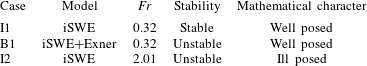

Figure 1. Growth rate of perturbations added to the reference case (tables 1 and 2) as a function of the wavenumber and the wavelength: (a–b) iSWE, $Fr<2$
(Case I1, well posed), (c–d) iSWE
$Fr<2$
(Case I1, well posed), (c–d) iSWE $+$
Exner (Case B1, well posed) and (e–f) iSWE,
$+$
Exner (Case B1, well posed) and (e–f) iSWE, $Fr>2$
(Case I2, ill posed). The panels in the two columns show the same information but highlight the behaviour for large wavenumbers (left column) and for large wavelengths (right column). Red and green indicates growth and decay of perturbations, respectively.
$Fr>2$
(Case I2, ill posed). The panels in the two columns show the same information but highlight the behaviour for large wavenumbers (left column) and for large wavelengths (right column). Red and green indicates growth and decay of perturbations, respectively.
A system is unstable when perturbations to an equilibrium state grow and the solution diverges from the initial equilibrium state. The growth of river bars is an example of an unstable system in river morphodynamics. A straight alluvial channel is stable if the width-to-depth ratio is sufficiently small and, above a certain threshold value, the channel becomes unstable and free alternate bars grow (Engelund & Skovgaard Reference Engelund and Skovgaard1973; Fredsøe Reference Fredsøe1978; Colombini, Seminara & Tubino Reference Colombini, Seminara and Tubino1987; Schielen et al.
Reference Schielen, Doelman and de Swart1993). Mathematically, an unstable system has a region, a domain in the wavenumber space, in which the growth rate of perturbations is positive. In figure 1(c,d) we present the growth rate of perturbations to a reference solution consisting of uniform flow (table 1) on an alluvial bed composed of unisize sediment with a characteristic grain size equal to 0.001 m (Case B1, table 2). The sediment transport rate is computed using the relation by Engelund & Hansen (Reference Engelund and Hansen1967) (B 4) and the effect of the bed slope on the sediment transport direction is accounted for using the simplest formulation, $g_{s}=1$
. Figure 1(d) confirms the classical result of linear bar theory: there exists a critical transverse wavelength (
$g_{s}=1$
. Figure 1(d) confirms the classical result of linear bar theory: there exists a critical transverse wavelength ( $l_{wyc}$
) below which all perturbations decay. In our particular case
$l_{wyc}$
) below which all perturbations decay. In our particular case $l_{wyc}=40.2~\text{m}$
. Impermeable boundary conditions at the river banks limit the possible wavelengths to fractions of the channel width
$l_{wyc}=40.2~\text{m}$
. Impermeable boundary conditions at the river banks limit the possible wavelengths to fractions of the channel width $B$
(m) such that
$B$
(m) such that $l_{wy}=2B/m$
for
$l_{wy}=2B/m$
for $m=1,2,\ldots$
(Callander Reference Callander1969). As the most unstable mode is the first one (i.e.
$m=1,2,\ldots$
(Callander Reference Callander1969). As the most unstable mode is the first one (i.e. $m=1$
, alternate bars) (Colombini et al.
Reference Colombini, Seminara and Tubino1987; Schielen et al.
Reference Schielen, Doelman and de Swart1993), the minimum channel width above which perturbations grow is
$m=1$
, alternate bars) (Colombini et al.
Reference Colombini, Seminara and Tubino1987; Schielen et al.
Reference Schielen, Doelman and de Swart1993), the minimum channel width above which perturbations grow is $B_{c}=l_{wyc}/2=20.1~\text{m}$
, which confirms the results of Schielen et al. (Reference Schielen, Doelman and de Swart1993). Figure 1(c) highlights, as for Case I1, the decay of short waves.
$B_{c}=l_{wyc}/2=20.1~\text{m}$
, which confirms the results of Schielen et al. (Reference Schielen, Doelman and de Swart1993). Figure 1(c) highlights, as for Case I1, the decay of short waves.
A particular case of instability is that in which the domain of positive growth rate extends to infinitely large wavenumbers (i.e. short waves). Under this condition there is no cutoff wavenumber above which we can neglect the contribution of ever shorter waves with non-zero growth rates. For any unstable perturbation a shorter one can be found which is even more unstable. This implies that the growth rate of an infinitesimal perturbation (i.e. noise) tends to infinity. Such a system cannot represent a physical phenomenon, as the growth rate of any physical process in nature is bounded. A system in which the growth rate of infinitesimal perturbations tends to infinity does not have a unique solution depending continuously on the initial and boundary conditions, which implies that the system is ill posed (Hadamard Reference Hadamard1923; Joseph & Saut Reference Joseph and Saut1990). An example of an ill-posed hydrodynamic model is the iSWE for flow with a Froude number larger than 2. In figure 1(e,f) we show the growth rate of perturbations to the reference solution of a case in which the Froude number is slightly larger than 2 (Case I2, table 2). The growth rate extends to infinitely large wavenumbers, which confirms that this case is ill posed. A model being ill posed is an indication that there is a relevant physical mechanism that has been neglected in the model derivation (Fowler Reference Fowler1997). Viscous forces regularise the iSWE (i.e. make the model well posed) and rather than ill posed, the viscous shallow water equations become simply unstable for a Froude number larger than 2, predicting the formation of roll waves (Balmforth & Mandre Reference Balmforth and Mandre2004; Balmforth & Vakil Reference Balmforth and Vakil2012; Rodrigues & Zumbrun Reference Rodrigues and Zumbrun2016; Barker et al. Reference Barker, Johnson, Noble, Rodrigues and Zumbrun2017a ,Reference Barker, Johnson, Noble, Rodrigues and Zumbrun b ).
Chaotic models, just as ill-posed models, are sensitive to the initial and boundary conditions and lose their predictive capabilities in a deterministic sense (Lorenz Reference Lorenz1963). Yet, there are two essential differences. First, chaotic systems lose their predictive capabilities after a certain time (Devaney Reference Devaney1989; Banks et al. Reference Banks, Brooks, Cairns, Davis and Stacey1992), yet there exists a finite time in which the dynamics is predictable. In ill-posed models infinitesimal perturbations to the initial condition cause a finite divergence in the solution in an arbitrarily (but fixed) short time. Second, while the dynamics of a chaotic model is not predictable in deterministic terms after a certain time, these continue to be predictable in statistical terms. For this reason, although being sensitive to the initial and boundary conditions, a model presenting chaotic properties can be used, for instance, to capture the essential dynamics and spatio-temporal features of river braiding (Murray & Paola Reference Murray and Paola1994, Reference Murray and Paola1997). On the contrary, the dynamics of an ill-posed model cannot be analysed in statistical terms.
The numerical solution of an ill-posed problem continues to change as the grid is refined because a smaller grid size resolves larger wavenumbers with faster growth rates (Joseph & Saut Reference Joseph and Saut1990; Kabanikhin Reference Kabanikhin2008; Barker et al. Reference Barker, Schaeffer, Bohorquez and Gray2015; Woodhouse et al. Reference Woodhouse, Thornton, Johnson, Kokelaar and Gray2012). In other words, the numerical solution of an ill-posed problem does not converge when the grid cell size is reduced. This property emphasises the unrealistic nature of ill-posed problems and shows that ill-posed models cannot be applied in practice.
We present an example of grid dependence specifically related to river morphodynamics under conditions with mixed-size sediment. We consider a case of degradation into a substrate finer than the active layer, as this is a situation in which the active layer model is prone to be ill posed (§ 1). The reference state is the same as in Case B1, yet the sediment is a mixture of two sizes equal to 0.001 m and 0.010 m. The bed surface is composed of 10 % fine sediment. The active layer thickness is equal to 0.05 m, which in this case is representative of small dunes covering the bed (e.g. Deigaard & Fredsøe Reference Deigaard and Fredsøe1978; Armanini & di Silvio Reference Armanini and di Silvio1988; Blom Reference Blom2008). Depending on the substrate composition, this situation yields an ill-posed model (Chavarrías et al. Reference Chavarrías, Stecca and Blom2018). When the substrate is composed of 50 % fine sediment (Case H1, table 3), the problem is well posed and it is ill posed when the substrate is composed of 90 % fine sediment (Case H2, table 3).
We use the software package Delft3D (Lesser et al.
Reference Lesser, Roelvink, van Kester and Stelling2004) to solve the system of equations. We stress that the problem of ill posedness is inherent to the system of equations and independent from the numerical solver. We have implemented a subroutine that assesses the well posedness of the system of equations at each node and time step. The domain is 100 m long and 10 m wide. The downstream water level is lowered at a rate of $0.01~\text{m}~\text{h}^{-1}$
to induce degradational conditions. The upstream sediment load is constant and equal to the equilibrium value of the reference state (Blom et al.
Reference Blom, Arkesteijn, Chavarrías and Viparelli2017). The cells are square and we consider three different sizes (table 3). The time step varies between simulations to maintain a constant value of the CFL (Courant, Friedrichs & Lewy Reference Courant, Friedrichs and Lewy1928) number.
$0.01~\text{m}~\text{h}^{-1}$
to induce degradational conditions. The upstream sediment load is constant and equal to the equilibrium value of the reference state (Blom et al.
Reference Blom, Arkesteijn, Chavarrías and Viparelli2017). The cells are square and we consider three different sizes (table 3). The time step varies between simulations to maintain a constant value of the CFL (Courant, Friedrichs & Lewy Reference Courant, Friedrichs and Lewy1928) number.
Table 3. Cases showing the effect of grid cell size on the numerical solution of well-posed and ill-posed models.
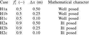
Figure 2 presents the bed elevation after 10 h. The result of the well-posed case (H1, left column) is grid independent. The result of the ill-posed case (H2, right column) changes as the grid is refined and presents an oscillatory pattern characteristic of ill-posed simulations (Joseph & Saut Reference Joseph and Saut1990; Woodhouse et al. Reference Woodhouse, Thornton, Johnson, Kokelaar and Gray2012; Barker et al. Reference Barker, Schaeffer, Bohorquez and Gray2015; Chavarrías et al. Reference Chavarrías, Stecca and Blom2018). The bed seems to be flat in the ill-posed simulation with a coarser grid (figure 2 b). This is because oscillations grow slowly on a coarse grid and require more time to be perceptible. The waviness of the bed is seen in the result of the check routine, as it predicts ill posedness only at those locations where the bed degrades (the stoss face of the oscillations). The fact that the model is well posed in almost the entire domain in the ill-posed case solved using a cell size equal to 0.25 m (H2b, figure 2 d) and 0.10 m (H2c, figure 2 f) does not mean that the results are realistic. Non-physical oscillations have grown and vertically mixed the sediment such that the situation is well posed after 10 h (Chavarrías et al. Reference Chavarrías, Stecca and Blom2018). We provide a movie of figure 2 in the online supplementary material available at https://doi.org/10.1017/jfm.2019.166.

Figure 2. Simulated bed elevation (surface) and mean grain size at the bed surface (colour) of a well-posed case (left column, H1, table 3) and an ill-posed case (right column, H2, table 3). In each row we present the results for varying cell size. The colour of the $x$
–
$x$
– $y$
plane shows the result of the routine that checks whether the conditions at each node yield a well-posed (green) or an ill-posed (red) model.
$y$
plane shows the result of the routine that checks whether the conditions at each node yield a well-posed (green) or an ill-posed (red) model.
In the above idealised situations it is evident that the oscillations are non-physical and it is straightforward to do a converge test to clarify that the solution is grid dependent. In complex domains in which several processes play a role, it is more difficult to associate oscillations with ill posedness. Moreover, in long term applications the growth rate of perturbations may be fast compared to the frequency at which model results are assessed, which may hide the consequences of ill posedness. If one studies a process that covers months or years (and consequently analyses the results on a monthly basis) but perturbations due to ill posedness grow on an hourly scale, it may be difficult to identify that the problem is ill posed. Using poor numerical techniques to solve the system of equations also contributes to hiding the consequences of ill posedness as numerical diffusion dampens perturbations. These factors may explain why the problem of ill posedness in mixed-sediment river morphodynamics is not widely acknowledged.
In the river morphodynamics community, the term ellipticity has been used to refer to the ill posedness of the system of equations in contrast to hyperbolicity, which is associated with well posedness (Ribberink Reference Ribberink1987; Mosselman Reference Mosselman, Bates, Lane and Ferguson2005; Stecca et al.
Reference Stecca, Siviglia and Blom2014; Siviglia, Stecca & Blom Reference Siviglia, Stecca, Blom, Tsutsumi and Laronne2017; Chavarrías et al.
Reference Chavarrías, Stecca and Blom2018). In general the terms are equivalent, but not always. We consider a unit vector $\hat{\boldsymbol{n}}$
in the direction
$\hat{\boldsymbol{n}}$
in the direction $(x,y)$
,
$(x,y)$
, $\hat{\boldsymbol{n}}=(\hat{n}_{x},\hat{n}_{y})$
. The system of equations (2.24) is hyperbolic if matrix
$\hat{\boldsymbol{n}}=(\hat{n}_{x},\hat{n}_{y})$
. The system of equations (2.24) is hyperbolic if matrix $\unicode[STIX]{x1D63C}=\unicode[STIX]{x1D63C}_{\boldsymbol{x}\mathbf{0}}\hat{n}_{x}+\unicode[STIX]{x1D63C}_{\boldsymbol{y}\mathbf{0}}\hat{n}_{y}$
diagonalises with real eigenvalues
$\unicode[STIX]{x1D63C}=\unicode[STIX]{x1D63C}_{\boldsymbol{x}\mathbf{0}}\hat{n}_{x}+\unicode[STIX]{x1D63C}_{\boldsymbol{y}\mathbf{0}}\hat{n}_{y}$
diagonalises with real eigenvalues $\forall \hat{n}$
(e.g. LeVeque Reference LeVeque2004; Castro et al.
Reference Castro, Fernández-Nieto, Ferreiro, García-Rodríguez and Parés2009). Neglecting friction and diffusive processes (i.e.
$\forall \hat{n}$
(e.g. LeVeque Reference LeVeque2004; Castro et al.
Reference Castro, Fernández-Nieto, Ferreiro, García-Rodríguez and Parés2009). Neglecting friction and diffusive processes (i.e. $\unicode[STIX]{x1D63D}_{\mathbf{0}}=\unicode[STIX]{x1D63F}_{\boldsymbol{x}\mathbf{0}}=\unicode[STIX]{x1D63F}_{\boldsymbol{y}\mathbf{0}}=\mathbb{0}$
), hyperbolicity implies that the eigenvalues of
$\unicode[STIX]{x1D63D}_{\mathbf{0}}=\unicode[STIX]{x1D63F}_{\boldsymbol{x}\mathbf{0}}=\unicode[STIX]{x1D63F}_{\boldsymbol{y}\mathbf{0}}=\mathbb{0}$
), hyperbolicity implies that the eigenvalues of $\unicode[STIX]{x1D648}_{\mathbf{0}}$
(2.33) are real. In this case, as the growth rate of perturbations (i.e. the imaginary part of the eigenvalues of
$\unicode[STIX]{x1D648}_{\mathbf{0}}$
(2.33) are real. In this case, as the growth rate of perturbations (i.e. the imaginary part of the eigenvalues of $\unicode[STIX]{x1D648}_{\mathbf{0}}$
) is equal to 0 regardless of the wavenumber, the system of equations is well posed. As the coefficients of
$\unicode[STIX]{x1D648}_{\mathbf{0}}$
) is equal to 0 regardless of the wavenumber, the system of equations is well posed. As the coefficients of $\unicode[STIX]{x1D63C}$
are real, complex eigenvalues appear in conjugate pairs. This means that if
$\unicode[STIX]{x1D63C}$
are real, complex eigenvalues appear in conjugate pairs. This means that if $\unicode[STIX]{x1D63C}$
has a complex eigenvalue (i.e. the problem is not hyperbolic), at least one wave will have a positive growth rate. Neglecting friction and diffusive processes, non-hyperbolicity implies that infinitely large wavenumbers have a positive growth rate. We conclude that, in the absence of diffusion and friction, lack of hyperbolicity implies ill posedness. Note that ellipticity (i.e. the eigenvalues of
$\unicode[STIX]{x1D63C}$
has a complex eigenvalue (i.e. the problem is not hyperbolic), at least one wave will have a positive growth rate. Neglecting friction and diffusive processes, non-hyperbolicity implies that infinitely large wavenumbers have a positive growth rate. We conclude that, in the absence of diffusion and friction, lack of hyperbolicity implies ill posedness. Note that ellipticity (i.e. the eigenvalues of $\unicode[STIX]{x1D63C}$
are all complex) is not required for the problem to be ill posed, as it suffices that the problem is not hyperbolic. When considering diffusion and friction even when
$\unicode[STIX]{x1D63C}$
are all complex) is not required for the problem to be ill posed, as it suffices that the problem is not hyperbolic. When considering diffusion and friction even when $\unicode[STIX]{x1D63C}$
has complex eigenvalues, the imaginary part of the eigenvalues of
$\unicode[STIX]{x1D63C}$
has complex eigenvalues, the imaginary part of the eigenvalues of $\unicode[STIX]{x1D648}_{\mathbf{0}}$
may all be negative and the problem well posed.
$\unicode[STIX]{x1D648}_{\mathbf{0}}$
may all be negative and the problem well posed.
Finally, well posedness and hyperbolicity are similar terms when dealing with problems arising from conservation laws and changes with time, as hyperbolicity guarantees the existence of wave solutions (Lax Reference Lax1980; Courant & Hilbert Reference Courant and Hilbert1989; Strikwerda Reference Strikwerda2004; Toro Reference Toro2009; Dafermos Reference Dafermos2010; Bressan Reference Bressan and Meyers2011; Dafermos Reference Dafermos, Abgrall and Shu2016). In communities such as materials science, it is the term hyperbolicity that is associated with ill posedness, as a smooth solution of, for instance the stress, requires that the system is elliptic (Knowles & Sternberg Reference Knowles and Sternberg1975, Reference Knowles and Sternberg1976; Veprek, Steiger & Witzigmann Reference Veprek, Steiger and Witzigmann2007).
4 Stability analysis
In this section we study the applicability of the system of equations to model two-dimensional river morphodynamics by means of a stability analysis of perturbations. We study the effects of the secondary flow model (§ 4.1) and the bed slope (§ 4.2) on model ill posedness.
4.1 Ill posedness due to secondary flow
In this section we study how the stability of the system of equations is affected by the secondary flow model. To gain insight we compare three cases. In the first case we omit secondary flow. In the second and third cases we include the secondary flow model with and without considering diffusion (table 4).
Table 4. Variations to the reference state (table 1) and results of the linear analysis with respect to secondary flow.
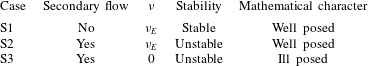
The first case is equivalent to I1 (table 2), yet the eddy viscosity is equal to the value derived by Elder ((2.4), $\unicode[STIX]{x1D708}=\unicode[STIX]{x1D708}_{E}=0.0057~\text{m}^{2}~\text{s}^{-1}$
). In figure 3(a,b) we plot the maximum growth rate of perturbations as a function of the wavenumber and the wavelength, respectively. Diffusion appears to significantly dampen perturbations (compare figure 1(a) in which diffusion is neglected to figure 3
a).
$\unicode[STIX]{x1D708}=\unicode[STIX]{x1D708}_{E}=0.0057~\text{m}^{2}~\text{s}^{-1}$
). In figure 3(a,b) we plot the maximum growth rate of perturbations as a function of the wavenumber and the wavelength, respectively. Diffusion appears to significantly dampen perturbations (compare figure 1(a) in which diffusion is neglected to figure 3
a).

Figure 3. Growth rate of perturbations added to the reference case (tables 1 and 4) as a function of the wavenumber and the wavelength: (a,b) without secondary flow (Case S1, well posed), (c,d) accounting for secondary flow with diffusion (Case S2, well posed) and (e,f) accounting for secondary flow without diffusion (Case S3, ill posed). The panels in the two columns show the same information but highlight the behaviour for large wavenumbers (a,c,e) and for large wavelengths (b,d,f). Red and green indicate growth and decay of perturbations, respectively.
In the second case we repeat the analysis including the equation for advection and diffusion of the secondary flow intensity (i.e. the first four rows and columns of matrix $\unicode[STIX]{x1D648}_{\mathbf{0}}$
in (2.33), Case S2, table 4). We observe that accounting for secondary flow introduces an instability mechanism (figure 3
d). For the specific conditions of the case, a growth domain appears for wavelengths between 0.7 m and 39 m long and between 0.4 m and 19 m wide. The maximum growth corresponds to a wavelength in the
$\unicode[STIX]{x1D648}_{\mathbf{0}}$
in (2.33), Case S2, table 4). We observe that accounting for secondary flow introduces an instability mechanism (figure 3
d). For the specific conditions of the case, a growth domain appears for wavelengths between 0.7 m and 39 m long and between 0.4 m and 19 m wide. The maximum growth corresponds to a wavelength in the $x$
and
$x$
and $y$
direction equal to 1.29 m and 0.74 m, respectively. This situation is well posed, as for large wavenumbers perturbations decay (figure 3
c). Yet, the model is unsuitable for reproducing such instability, as it predicts growth of perturbations with a length scale of the order of the flow depth and shorter, for which the shallow water equation model is not suited. Given the fact that we consider a depth-averaged formulation of the primary flow, processes that scale with the flow depth are not resolved by the model and consequently perturbations at that scale must decay to yield physically realistic results. Otherwise, scales of the order of the flow depth become relevant, which contradicts the assumptions of the depth-averaged formulation. To model processes that scale with the flow depth such as dune growth, it is necessary to account for non-depth-averaged flow formulations that consider, for instance, rotational flow (Colombini & Stocchino Reference Colombini and Stocchino2011, Reference Colombini and Stocchino2012), or non-hydrostatic pressure (Giri & Shimizu Reference Giri and Shimizu2006; Shimizu et al.
Reference Shimizu, Giri, Yamaguchi and Nelson2009).
$y$
direction equal to 1.29 m and 0.74 m, respectively. This situation is well posed, as for large wavenumbers perturbations decay (figure 3
c). Yet, the model is unsuitable for reproducing such instability, as it predicts growth of perturbations with a length scale of the order of the flow depth and shorter, for which the shallow water equation model is not suited. Given the fact that we consider a depth-averaged formulation of the primary flow, processes that scale with the flow depth are not resolved by the model and consequently perturbations at that scale must decay to yield physically realistic results. Otherwise, scales of the order of the flow depth become relevant, which contradicts the assumptions of the depth-averaged formulation. To model processes that scale with the flow depth such as dune growth, it is necessary to account for non-depth-averaged flow formulations that consider, for instance, rotational flow (Colombini & Stocchino Reference Colombini and Stocchino2011, Reference Colombini and Stocchino2012), or non-hydrostatic pressure (Giri & Shimizu Reference Giri and Shimizu2006; Shimizu et al.
Reference Shimizu, Giri, Yamaguchi and Nelson2009).
In the third case we test the secondary flow model without accounting for diffusion in the system of equations ( $\unicode[STIX]{x1D708}=0$
, Case S3, table 4). We observe that the instability domain extends to infinitely large wavenumbers (figure 3
e), which implies that this model is ill posed (§ 3). We now aim to prove that the shallow water equations in combination with the secondary flow model without diffusion always yields an ill-posed model. To this end we obtain the characteristic polynomial of matrix
$\unicode[STIX]{x1D708}=0$
, Case S3, table 4). We observe that the instability domain extends to infinitely large wavenumbers (figure 3
e), which implies that this model is ill posed (§ 3). We now aim to prove that the shallow water equations in combination with the secondary flow model without diffusion always yields an ill-posed model. To this end we obtain the characteristic polynomial of matrix $\unicode[STIX]{x1D648}_{\mathbf{0}}$
(2.33). We compute the discriminant of the fourth-order characteristic polynomial and we find that for
$\unicode[STIX]{x1D648}_{\mathbf{0}}$
(2.33). We compute the discriminant of the fourth-order characteristic polynomial and we find that for $k_{wx}<k_{wy}$
the growth rate of perturbations is positive (appendix C). The model is ill posed, as there always exists a domain of growth extending to infinitely large wavenumbers in the transverse direction.
$k_{wx}<k_{wy}$
the growth rate of perturbations is positive (appendix C). The model is ill posed, as there always exists a domain of growth extending to infinitely large wavenumbers in the transverse direction.
We assess how the length scale of the instability related to the secondary flow model depends on the flow parameters. For this purpose we compute the shortest wave with positive growth for a varying diffusion coefficient and flow conditions (figure 4). We observe that, independently of the flow conditions, the theoretical value of the diffusion coefficient derived by Elder (Reference Elder1959) (2.4) is insufficient for dampening oscillations scaling with the flow depth. We conclude that if the diffusion coefficient is realistic, the treatment of the secondary flow yields an unrealistic model. It is necessary to use an unrealistically large value of the diffusion coefficient to obtain a realistic depth-averaged model in which perturbations scaling with the flow depth decay.

Figure 4. Wavelength of the shortest perturbation with positive growth rate ( $l_{wm}$
) relative to the flow depth (
$l_{wm}$
) relative to the flow depth ( $h$
) as a function of the Froude number (
$h$
) as a function of the Froude number ( $Fr$
) and the diffusion coefficient (
$Fr$
) and the diffusion coefficient ( $\unicode[STIX]{x1D708}$
) relative to the diffusion coefficient according to Elder (Reference Elder1959) (
$\unicode[STIX]{x1D708}$
) relative to the diffusion coefficient according to Elder (Reference Elder1959) ( $\unicode[STIX]{x1D708}_{E}$
). Different flow conditions are studied varying the flow depth between 0.2 m and 1.5 m from the reference case (table 1). The cyan markers indicate the conditions of three numerical simulations with different values of the diffusion coefficient (§ 5.1). The arrow next to the diamond marker indicates that the value lies outside the figure. Red (green) colour indicates that the shortest wavelength with positive growth rate are smaller (larger) than the flow depth.
$\unicode[STIX]{x1D708}_{E}$
). Different flow conditions are studied varying the flow depth between 0.2 m and 1.5 m from the reference case (table 1). The cyan markers indicate the conditions of three numerical simulations with different values of the diffusion coefficient (§ 5.1). The arrow next to the diamond marker indicates that the value lies outside the figure. Red (green) colour indicates that the shortest wavelength with positive growth rate are smaller (larger) than the flow depth.
4.2 Ill posedness due to bed slope effect
In this section we study the influence of considering the effect of the bed slope on model well posedness. To gain insight we compare five cases in which we consider unisize and mixed-size sediment, various sediment transport relations and various bed slope functions (table 5). We neglect secondary flow and diffusion to reduce the complexity of the problem (Parker Reference Parker1976; Fredsøe Reference Fredsøe1978; Colombini et al. Reference Colombini, Seminara and Tubino1987; Schielen et al. Reference Schielen, Doelman and de Swart1993).
Our reference case is B1 (§ 3) which considers unisize sediment conditions, and the effect of the bed slope on the sediment transport direction is accounted for using the simplest formulation, $g_{s}=1$
. We have shown that this case is well posed. Neglecting the effect of the bed slope on the sediment transport direction (Case B2, table 5) makes the problem ill posed (figure 5
a). This illustrates that accounting for the effect of the bed slope is required for obtaining not only physically realistic but also mathematically well-posed results. We prove that the shallow water equations in combination with the Exner (Reference Exner1920) equation without considering the effect of the bed slope always yields an ill-posed model by studying the growth rate of perturbations in the limit as the wavenumber
$g_{s}=1$
. We have shown that this case is well posed. Neglecting the effect of the bed slope on the sediment transport direction (Case B2, table 5) makes the problem ill posed (figure 5
a). This illustrates that accounting for the effect of the bed slope is required for obtaining not only physically realistic but also mathematically well-posed results. We prove that the shallow water equations in combination with the Exner (Reference Exner1920) equation without considering the effect of the bed slope always yields an ill-posed model by studying the growth rate of perturbations in the limit as the wavenumber $k_{wy}$
tends to infinity (appendix D).
$k_{wy}$
tends to infinity (appendix D).

Figure 5. Growth rate of perturbations added to the reference case (tables 1 and 5) as a function of the wavenumber and the wavelength: (a,b) Case B2 (ill posed), (c,d) Case B3 (well posed), (e,f) Case B4 (ill posed) and (g,h) Case B5 (ill posed). The panels in the two columns show the same information but highlight the behaviour for large wavenumbers (a,c,e,g) and for large wavelengths (b,d,f,h). Red and green indicate growth and decay of perturbations, respectively.
Table 5. Variations to the reference state (table 1) and results of the linear analysis with respect to the effect of the bed slope on the sediment transport direction. EH and AM refer to the sediment transport relations by Engelund & Hansen (Reference Engelund and Hansen1967) and Ashida & Michiue (Reference Ashida and Michiue1971), respectively.
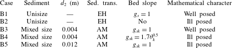
The fact that the bed slope effect dampens perturbations under unisize conditions is expected from the fact that the only diffusive term in the system of equations is $\unicode[STIX]{x2202}q_{by}/\unicode[STIX]{x2202}s_{y}$
(2.27), where
$\unicode[STIX]{x2202}q_{by}/\unicode[STIX]{x2202}s_{y}$
(2.27), where $s_{y}=\unicode[STIX]{x2202}\unicode[STIX]{x1D702}/\unicode[STIX]{x2202}y$
. This term is negative and approximately equal to
$s_{y}=\unicode[STIX]{x2202}\unicode[STIX]{x1D702}/\unicode[STIX]{x2202}y$
. This term is negative and approximately equal to $-q_{b}/g_{s}$
for a small streamwise slope. When we consider more than one grain size, diffusive terms appear in each active layer equation. We find that these diffusive terms may be positive, which hints at the possibility of an antidiffusive behaviour, which may lead to ill posedness. To study this possibility we compute the growth rate of perturbations of a simplified case consisting of two sediment size fractions. In the limit for the wavenumbers tending to infinity, the maximum growth rate is:
$-q_{b}/g_{s}$
for a small streamwise slope. When we consider more than one grain size, diffusive terms appear in each active layer equation. We find that these diffusive terms may be positive, which hints at the possibility of an antidiffusive behaviour, which may lead to ill posedness. To study this possibility we compute the growth rate of perturbations of a simplified case consisting of two sediment size fractions. In the limit for the wavenumbers tending to infinity, the maximum growth rate is:
 $$\begin{eqnarray}\displaystyle \unicode[STIX]{x1D714}_{i}^{lim}=\unicode[STIX]{x1D6FC}_{1}(r_{y1}-d_{x1,1})^{2}+\unicode[STIX]{x1D6FC}_{2}(r_{y1}-d_{x1,1})+\unicode[STIX]{x1D6FC}_{3}, & & \displaystyle\end{eqnarray}$$
where $\unicode[STIX]{x1D6FC}_{i}$
for
$\unicode[STIX]{x1D6FC}_{i}$
for $i=1,2,3$
are parameters relating the flow and the sediment transport rate (appendix E). The parameter
$i=1,2,3$
are parameters relating the flow and the sediment transport rate (appendix E). The parameter $r_{y1}$
explains how the sediment transport rate of the fine fraction is affected by changes in the transverse bed slope:
$r_{y1}$
explains how the sediment transport rate of the fine fraction is affected by changes in the transverse bed slope:
 $$\begin{eqnarray}\displaystyle r_{y1}=\frac{\unicode[STIX]{x2202}q_{by1}/\unicode[STIX]{x2202}s_{y}}{\unicode[STIX]{x2202}q_{by}/\unicode[STIX]{x2202}s_{y}}, & & \displaystyle\end{eqnarray}$$
and the parameter $d_{x1,1}$
relates changes in the sediment transport rate to changes in the volume of sediment in the active layer:
$d_{x1,1}$
relates changes in the sediment transport rate to changes in the volume of sediment in the active layer:
 $$\begin{eqnarray}\displaystyle d_{x1,1}=\frac{\unicode[STIX]{x2202}q_{bx1}/\unicode[STIX]{x2202}M_{a1}}{\unicode[STIX]{x2202}q_{bx}/\unicode[STIX]{x2202}M_{a1}}. & & \displaystyle\end{eqnarray}$$
As $\unicode[STIX]{x1D6FC}_{1}>0$
(appendix E), there exists an interval
$\unicode[STIX]{x1D6FC}_{1}>0$
(appendix E), there exists an interval $(r_{y1}-d_{x1,1})^{-}<(r_{y1}-d_{x1,1})<(r_{y1}-d_{x1,1})^{+}$
in which
$(r_{y1}-d_{x1,1})^{-}<(r_{y1}-d_{x1,1})<(r_{y1}-d_{x1,1})^{+}$
in which $\unicode[STIX]{x1D714}_{i}^{lim}<0$
and the model is well posed. Outside the interval,
$\unicode[STIX]{x1D714}_{i}^{lim}<0$
and the model is well posed. Outside the interval, $\unicode[STIX]{x1D714}_{i}^{lim}>0$
and the problem is ill posed.
$\unicode[STIX]{x1D714}_{i}^{lim}>0$
and the problem is ill posed.
The physical interpretation of the limit values for obtaining a well-posed model is as follows. The effect of the transverse bed slope ( $r_{y1}$
) needs to be balanced with respect to the effect of changes in surface texture (
$r_{y1}$
) needs to be balanced with respect to the effect of changes in surface texture ( $d_{x1,1}$
) to obtain a well-posed model. For a given
$d_{x1,1}$
) to obtain a well-posed model. For a given $d_{x1,1}$
, if parameter
$d_{x1,1}$
, if parameter $r_{y1}$
is too small (i.e. the bed slope effect is not sufficiently strong) perturbations in the transverse direction are not dampened and the model is ill posed. On the other hand, for a given
$r_{y1}$
is too small (i.e. the bed slope effect is not sufficiently strong) perturbations in the transverse direction are not dampened and the model is ill posed. On the other hand, for a given $r_{y1}$
, if parameter
$r_{y1}$
, if parameter $d_{x1,1}$
is too small (e.g. due to relatively strong hiding or in conditions close to incipient motion) perturbations in the streamwise direction do not decay and the model is also ill posed. The critical values
$d_{x1,1}$
is too small (e.g. due to relatively strong hiding or in conditions close to incipient motion) perturbations in the streamwise direction do not decay and the model is also ill posed. The critical values $r_{y1}^{\pm }$
that allow for a well-posed model are shown in appendix E.
$r_{y1}^{\pm }$
that allow for a well-posed model are shown in appendix E.
In Cases B3–B5 we illustrate the possibility of ill posedness due to the bed slope closure relation (table 5). In Case B3 the sediment mixture consists of two grain size fractions with characteristic grain sizes equal to 0.001 m and 0.004 m. The volume fraction content of the fine sediment in the active layer and at the interface between the active layer and the substrate is equal to 0.5. The sediment transport rate is computed using the relation developed by Ashida & Michiue (Reference Ashida and Michiue1971). The other parameters are equal to the reference case (table 1). The system is well posed when the effect of the bed slope does not depend on the bed shear stress (figure 5 c). The situation is ill posed if the effect of the bed slope depends on the bed shear stress (Case B4, table 5, figure 5 e). The cause of the ill posedness is not found in the closure relation for the bed slope effect only but in the combination of the closure relation with the flow and bed surface conditions. A case equal to B3 except for the fact that the coarse grain size is equal to 0.012 m is ill posed (Case B5, table 5, figure 5 g).
We assess how the domain of ill posedness due to the bed slope effect depends on the model parameters. For given sediment sizes, flow and bed surface texture, parameter $B_{s}$
(2.23) controls the effect of the bed slope by modifying
$B_{s}$
(2.23) controls the effect of the bed slope by modifying $r_{y1}$
only. The parameter
$r_{y1}$
only. The parameter $A_{s}$
(2.23) cancels in
$A_{s}$
(2.23) cancels in $r_{y1}$
and does not play a role. For this reason we study how
$r_{y1}$
and does not play a role. For this reason we study how $g_{s1}/A_{s}$
(
$g_{s1}/A_{s}$
( $-$
) affects the domain of ill posedness for varying sediment properties, flow and bed surface grain size distribution (figure 6). We consider Case B3 and we vary
$-$
) affects the domain of ill posedness for varying sediment properties, flow and bed surface grain size distribution (figure 6). We consider Case B3 and we vary $B_{s}$
between 0 and 0.5 to vary the bed slope effect. The sediment size of the coarse fraction varies between
$B_{s}$
between 0 and 0.5 to vary the bed slope effect. The sediment size of the coarse fraction varies between $d_{1}$
and 0.020 m. The mean flow velocity varies between
$d_{1}$
and 0.020 m. The mean flow velocity varies between $1~\text{m}~\text{s}^{-1}$
and
$1~\text{m}~\text{s}^{-1}$
and $2.8~\text{m}~\text{s}^{-1}$
. The volume fraction content of fine sediment at the bed surface varies between 0 and 1. We aim to isolate the problem of ill posedness due to bed slope effect from the problem of ill posedness due to a different grain size distribution at the bed surface and at the interface between the bed surface and the substrate (Chavarrías et al.
Reference Chavarrías, Stecca and Blom2018). For this reason, in this analysis the volume fraction content of fine sediment at the interface is equal to the one at the bed surface. Under this condition the problem can be ill posed due to the effect of the bed slope only.
$2.8~\text{m}~\text{s}^{-1}$
. The volume fraction content of fine sediment at the bed surface varies between 0 and 1. We aim to isolate the problem of ill posedness due to bed slope effect from the problem of ill posedness due to a different grain size distribution at the bed surface and at the interface between the bed surface and the substrate (Chavarrías et al.
Reference Chavarrías, Stecca and Blom2018). For this reason, in this analysis the volume fraction content of fine sediment at the interface is equal to the one at the bed surface. Under this condition the problem can be ill posed due to the effect of the bed slope only.
As we have shown analytically, under unisize conditions (i.e. $d_{1}/d_{2}=1$
or
$d_{1}/d_{2}=1$
or $F_{a1}=1$
or
$F_{a1}=1$
or $F_{a1}=0$
) the model is well posed (figure 6
a,c). For sufficiently different grain sizes (
$F_{a1}=0$
) the model is well posed (figure 6
a,c). For sufficiently different grain sizes ( $d_{1}/d_{2}\lessapprox 0.15$
) the model is well posed regardless of the bed slope effect but for a small range of values (
$d_{1}/d_{2}\lessapprox 0.15$
) the model is well posed regardless of the bed slope effect but for a small range of values ( $0.08\lessapprox d_{1}/d_{2}\lessapprox 0.1$
). This small range of ill-posed values is associated with
$0.08\lessapprox d_{1}/d_{2}\lessapprox 0.1$
). This small range of ill-posed values is associated with $r_{y1}$
increasing for decreasing values of
$r_{y1}$
increasing for decreasing values of $d_{1}/d_{2}$
and acquiring a value larger than
$d_{1}/d_{2}$
and acquiring a value larger than $r_{y1}^{+}$
such that the model becomes ill posed for all values of the bed slope effect. A further decrease in
$r_{y1}^{+}$
such that the model becomes ill posed for all values of the bed slope effect. A further decrease in $d_{1}/d_{2}$
increases the limit value
$d_{1}/d_{2}$
increases the limit value $r_{y1}^{+}$
faster than
$r_{y1}^{+}$
faster than $r_{y1}$
such that the model becomes well posed for all values of the bed slope effect.
$r_{y1}$
such that the model becomes well posed for all values of the bed slope effect.
An increase in the Froude number decreases the domain of well posedness, which is explained from the fact that an increase in Froude number decreases $r_{y1}$
while it does not modify
$r_{y1}$
while it does not modify $r_{y1}^{-}$
. We have assumed steady flow in deriving
$r_{y1}^{-}$
. We have assumed steady flow in deriving $\unicode[STIX]{x1D714}_{i}^{lim}$
to reduce the complexity of the model such that we can find an analytical solution (appendix E). This causes a physically unrealistic resonance phenomenon for
$\unicode[STIX]{x1D714}_{i}^{lim}$
to reduce the complexity of the model such that we can find an analytical solution (appendix E). This causes a physically unrealistic resonance phenomenon for $Fr\rightarrow 1$
(Colombini & Stocchino Reference Colombini and Stocchino2005). In reality we do not expect that for
$Fr\rightarrow 1$
(Colombini & Stocchino Reference Colombini and Stocchino2005). In reality we do not expect that for $Fr=1$
the model is always ill posed regardless of the bed slope effect. Apart from the limit values in which the problem becomes unisize, the surface volume fraction content does not significantly affect the domain of ill posedness (figure 6
c) as it rescales in more or less a similar way
$Fr=1$
the model is always ill posed regardless of the bed slope effect. Apart from the limit values in which the problem becomes unisize, the surface volume fraction content does not significantly affect the domain of ill posedness (figure 6
c) as it rescales in more or less a similar way $r_{y1}^{\pm }$
and
$r_{y1}^{\pm }$
and $r_{y1}$
.
$r_{y1}$
.
While Case B4 is ill posed because the effect of the bed slope ( $r_{y1}$
) is small, Case B5 is ill posed because parameter
$r_{y1}$
) is small, Case B5 is ill posed because parameter $d_{x1,1}$
is small. The different origin of ill posedness does not cause a significant difference in the growth rate of perturbations as a function of the wavenumber (figure 5
e–g). However, we will find out that the pattern resulting from the perturbations depends on the origin of the ill posedness.
$d_{x1,1}$
is small. The different origin of ill posedness does not cause a significant difference in the growth rate of perturbations as a function of the wavenumber (figure 5
e–g). However, we will find out that the pattern resulting from the perturbations depends on the origin of the ill posedness.

Figure 6. Domain of ill posedness due to the bed slope effect under mixed-size sediment conditions: as a function of the ratio between fine and coarse sediment (a), the Froude number (b) and the volume fraction content of fine sediment in the active layer (c). The bed slope effect is measured by $g_{s1}/A_{s}$
and the range of parameters is obtained by varying
$g_{s1}/A_{s}$
and the range of parameters is obtained by varying $B_{s}$
(2.23). The range of values of
$B_{s}$
(2.23). The range of values of $d_{1}/d_{2}$
is obtained by varying
$d_{1}/d_{2}$
is obtained by varying $d_{2}$
. The range of values of the Froude number is obtained by varying
$d_{2}$
. The range of values of the Froude number is obtained by varying $u$
. The volume fraction content of fine sediment at the interface between the active layer and the substrate is kept equal to the volume fraction content of fine sediment in the active layer. The conditions represent unisize sediment when
$u$
. The volume fraction content of fine sediment at the interface between the active layer and the substrate is kept equal to the volume fraction content of fine sediment in the active layer. The conditions represent unisize sediment when $d_{1}/d_{2}=1$
,
$d_{1}/d_{2}=1$
, $F_{a1}=0$
, or
$F_{a1}=0$
, or $F_{a1}=1$
.
$F_{a1}=1$
.
5 Application
The results of the linear stability analysis (§ 4) neglect second-order terms and nonlinear interactions. In this section we study the effects of the terms neglected in the linear analysis and the development of perturbations by means of numerical simulations. We use the software package Delft3D (Lesser et al. Reference Lesser, Roelvink, van Kester and Stelling2004). This exercise provides information on the consequences of ill posedness in numerical simulations and clarifies the limitations of the current modelling approach. We study the effect of secondary flow (§ 5.1) and the bed slope effect (§ 5.2).
5.1 Secondary flow
We run five numerical simulations with a fixed bed (i.e. only the flow is computed) to study the roles of the secondary flow model and the diffusion coefficient in the ill posedness of the system of equations. The first three simulations reproduce the conditions of Cases S1, S2 and S3 (table 4). The domain is rectangular, 100 m long and 10 m wide. We use square cells with size equal to 0.1 m. The time step is equal to 0.01 s and we simulate 10 min of flow. We set a constant water discharge and the downstream water level remains constant with time. The initial condition represents normal flow for the values in table 1 (i.e. equilibrium conditions).
The simulation not accounting for secondary flow does not present growth of perturbations as predicted by the linear analysis and remains stable with time (figure 7 a). We observe growth of perturbations when we account for secondary flow with the diffusion coefficient derived by Elder (Reference Elder1959) (figure 7 b). The results are physically unrealistic as the flow depth presents variations of up to 7 % of the normal flow depth and the length scale of the perturbations is smaller than the flow depth. We have not introduced any perturbation in the initial or boundary conditions which implies that perturbations grow from numerical truncation errors. This supports the fact that the simulation is physically unrealistic. The case with a diffusion coefficient equal to 0 is ill posed and the solution presents unreasonably large oscillations (figure 7 c). These numerical results confirm the results of the linear stability analysis.
In the fourth simulation we set a diffusion coefficient 100 times larger than the one derived by Elder (Reference Elder1959) (figure 7
d). Under this condition the linear analysis predicts all short waves to decay (diamond in figure 4). These numerical results confirm the linear theory. The last simulation is equal to Case S2 except for the fact that we use a coarser grid ( $\unicode[STIX]{x0394}x=\unicode[STIX]{x0394}y=1~\text{m}$
). In this case the numerical grid is not sufficiently detailed to resolve the perturbations due to secondary flow and the simulation is stable (figure 7
e). This last case highlights an important limitation of a physically unrealistic model. Although Case S2 is mathematically well posed, the solution presents similarities with ill-posed cases in the sense that a refinement of the grid causes non-physical oscillations to appear.
$\unicode[STIX]{x0394}x=\unicode[STIX]{x0394}y=1~\text{m}$
). In this case the numerical grid is not sufficiently detailed to resolve the perturbations due to secondary flow and the simulation is stable (figure 7
e). This last case highlights an important limitation of a physically unrealistic model. Although Case S2 is mathematically well posed, the solution presents similarities with ill-posed cases in the sense that a refinement of the grid causes non-physical oscillations to appear.

Figure 7. Flow depth at the end of the simulations: (a) without accounting for secondary flow (Case S1), (b) setting $\unicode[STIX]{x1D708}=\unicode[STIX]{x1D708}_{E}$
(Case S2), (c) setting
$\unicode[STIX]{x1D708}=\unicode[STIX]{x1D708}_{E}$
(Case S2), (c) setting $\unicode[STIX]{x1D708}=0$
(Case S3), (d) setting
$\unicode[STIX]{x1D708}=0$
(Case S3), (d) setting $\unicode[STIX]{x1D708}=100\unicode[STIX]{x1D708}_{E}$
and (e) setting
$\unicode[STIX]{x1D708}=100\unicode[STIX]{x1D708}_{E}$
and (e) setting $\unicode[STIX]{x1D708}=\unicode[STIX]{x1D708}_{E}$
using a coarser numerical grid (Case S2). The colour map is adjusted for each case and centred on the initial and equilibrium values (
$\unicode[STIX]{x1D708}=\unicode[STIX]{x1D708}_{E}$
using a coarser numerical grid (Case S2). The colour map is adjusted for each case and centred on the initial and equilibrium values ( $h=1~\text{m}$
).
$h=1~\text{m}$
).
5.2 Bed slope effect
In this section we focus on the consequences of accounting for the bed slope effect on the mathematical character of the model. To this end we run five more numerical simulations without accounting for secondary flow and updating the bed (i.e. accounting for morphodynamic change). The simulations reproduce Cases B1–B5 (table 5). We simulate 8 h using a time step $\unicode[STIX]{x0394}t=0.1~\text{s}$
.
$\unicode[STIX]{x0394}t=0.1~\text{s}$
.
We have proved that accounting for the effect of the bed slope makes a unisize simulation well posed (§ 4.2 and figure 1 c). The numerical solution of this case (B1, table 2) is stable and perturbations do not grow (figure 8 a). Moreover, no alternate bars appear as the channel width is below the critical value (§ 3). Perturbations grow when the effect of the bed slope is not taken into account (Case B2, figure 8 b), which confirms that this case is ill posed.

Figure 8. Flow depth at the end of the simulations of: (a) Case B1, (b) Case B2; and volume fraction content of fine sediment in the active layer: (c) Case B3, (d) Case B4, (e) Case B5. The colour map is adjusted for each case and centred on the initial and equilibrium values.
The mixed-size sediment conditions of Case B3 yield a well-posed model (figure 5
e) and the simulation is stable (figure 8
c). On the other hand, the ill-posed cases B4 and B5 present growth of unrealistic and non-physical perturbations (figure 8
d,e). While the growth of perturbations in Case B5 seems random, in Case B4 we observe a clear pattern. Moreover, oscillations have grown significantly faster in Case B5 than in Case B4. While after 8 h the changes in volume fraction content at the bed surface are of the order of $10^{-3}$
in Case B4, these are of order 1 in Case B5.
$10^{-3}$
in Case B4, these are of order 1 in Case B5.
The fact that oscillations grow faster in Case B5 than in Case B4 is related to the different origin of ill posedness. While Case B4 is ill posed because the effect of the bed slope is not sufficiently strong (i.e. $r_{y1}<r_{y1}^{-}$
), Case B5 is ill posed because changes in the sediment transport rate due to changes in the volume of fine sediment in the active layer are too small (i.e.
$r_{y1}<r_{y1}^{-}$
), Case B5 is ill posed because changes in the sediment transport rate due to changes in the volume of fine sediment in the active layer are too small (i.e. $r_{y1}>r_{y1}^{+}$
). The first case is closely linked to the lateral direction, in which sediment transport is initially zero. The fact that initially the lateral sediment transport rate is zero limits the rate at which lateral changes occur. In the second case perturbations are linked to the streamwise direction, in which the sediment transport rate initially is non-zero, which enhances the rate at which changes develop.
$r_{y1}>r_{y1}^{+}$
). The first case is closely linked to the lateral direction, in which sediment transport is initially zero. The fact that initially the lateral sediment transport rate is zero limits the rate at which lateral changes occur. In the second case perturbations are linked to the streamwise direction, in which the sediment transport rate initially is non-zero, which enhances the rate at which changes develop.
6 Discussion
The origin of the instability due to secondary flow is found in the source term ( $S_{s}$
in (2.11)). As the source term depends on the flow curvature, the source term is 0 in a straight flow. A small perturbation in the flow causes the flow to curve. The flow curvature causes a source of secondary flow intensity, which further increases the flow curvature, causing a positive feedback. The flow curvature is largest for the smallest perturbations, which explains why the model is ill posed if a dampening mechanism (i.e. diffusion) is not taken into account. This destabilising mechanism may seem plausible to explain secondary flow circulation observed in straight channels (Nikuradse Reference Nikuradse1930; Brundrett & Baines Reference Brundrett and Baines1964; Nezu & Nakagawa Reference Nezu and Nakagawa1984; Gavrilakis Reference Gavrilakis1992). However, secondary flow in a straight channel can only be caused by anisotropy of turbulence (Einstein & Li Reference Einstein and Li1958; Gessner & Jones Reference Gessner and Jones1965; Bradshaw Reference Bradshaw1987; Colombini Reference Colombini1993), which is not included in the model for secondary flow. For this reason, the secondary flow model must predict decay of secondary flow intensity in case of straight flow. Diffusion of secondary flow intensity causes decay of perturbations, but the theoretical diffusion coefficient derived by Elder (Reference Elder1959) appears to be insufficient to dampen perturbations.
$S_{s}$
in (2.11)). As the source term depends on the flow curvature, the source term is 0 in a straight flow. A small perturbation in the flow causes the flow to curve. The flow curvature causes a source of secondary flow intensity, which further increases the flow curvature, causing a positive feedback. The flow curvature is largest for the smallest perturbations, which explains why the model is ill posed if a dampening mechanism (i.e. diffusion) is not taken into account. This destabilising mechanism may seem plausible to explain secondary flow circulation observed in straight channels (Nikuradse Reference Nikuradse1930; Brundrett & Baines Reference Brundrett and Baines1964; Nezu & Nakagawa Reference Nezu and Nakagawa1984; Gavrilakis Reference Gavrilakis1992). However, secondary flow in a straight channel can only be caused by anisotropy of turbulence (Einstein & Li Reference Einstein and Li1958; Gessner & Jones Reference Gessner and Jones1965; Bradshaw Reference Bradshaw1987; Colombini Reference Colombini1993), which is not included in the model for secondary flow. For this reason, the secondary flow model must predict decay of secondary flow intensity in case of straight flow. Diffusion of secondary flow intensity causes decay of perturbations, but the theoretical diffusion coefficient derived by Elder (Reference Elder1959) appears to be insufficient to dampen perturbations.
The advection equation for the secondary flow intensity was initially derived for steady decaying secondary flow on a straight reach after a bend neglecting the effect of diffusion (De Vriend Reference de Vriend1981). It is assumed that the same advective behaviour is valid for a varying curvature (De Vriend Reference de Vriend1981; Olesen Reference Olesen1982) and in an unsteady situation (Booij & Pennekamp Reference Booij and Pennekamp1984). These assumptions have, to our knowledge, not been tested. Moreover, secondary flow affects the vertical profile of the primary flow. This feedback mechanism, which limits the development of secondary flow (Blanckaert & De Vriend Reference Blanckaert and de Vriend2004; Blanckaert Reference Blanckaert2009), is not included in the model. Blanckaert & De Vriend (Reference Blanckaert and de Vriend2003), Blanckaert & Graf (Reference Blanckaert and Graf2004) and Ottevanger et al. (Reference Ottevanger, Blanckaert, Uijttewaal and de Vriend2013) propose nonlinear models that take into consideration this mechanism. We expect that accounting for the feedback mechanism yields a well-posed model.
The feedback mechanism between the secondary and the primary flow may be seen as an increase of diffusivity, as it causes an enhanced momentum redistribution. For a situation in which the nonlinear model for the secondary flow appears to be excessively expensive in computational terms, a diffusion coefficient depending on the secondary flow intensity would (partially) account for the enhanced momentum redistribution and provide a well-posed and realistic model.
We have assumed that the diffusion coefficient is constant and equal in all directions, which is a crude approximation, as in the streamwise direction diffusion is larger than in the transverse direction (appendix A). It would be interesting to study the effect of anisotropic diffusion, however, we do not expect that this will significantly alter our results. This is because a larger diffusion coefficient in the streamwise direction will not alter the most unstable wavelength in the lateral direction. For this reason the shortest unstable waves remain of the order of the flow depth.
The nonlinear relation between the flow and the sediment transport rate causes the growth of perturbations in bed elevation. Worded differently, a deep flow attracts the flow and vice versa, which enhances the growth of perturbations. This mechanism is counteracted by the bed slope effect, which causes deep parts to fill in. In this sense, it seems logical that it is necessary to account for bed slope effects to obtain a well-posed model. This may be confirmed by the facts that Parker (Reference Parker1976), by not considering the bed slope effect, found that all streams tend to form bars and, similarly, Olesen (Reference Olesen1982) concluded that ‘the stream will develop an infinite number of submerged bars’. From our point of view the fact that all streams seem to be unstable and develop an infinite number of submerged bars is a consequence of the model being ill posed. Our analysis shows that the bed slope effect is a crucial physical process in analysing two-dimensional morphodynamic processes.
Nevertheless, the numerical simulations by Qian et al. (Reference Qian, Cao, Liu and Pender2016) for bar development without accounting for the bed slope effect do not show unrealistic oscillatory behaviour as is characteristic of ill posedness. Yet, there is an essential difference between their model and the one we analyse here. We do not model the interaction between the sediment in the bed and the sediment in transport as we assume that the sediment transport rate adapts instantaneously to changes in the flow (i.e. the sediment transport rate depends on the flow variables only). Essentially, sediment in transport is not conserved and bed elevation and surface texture changes depend on the divergence of the sediment transport rate at capacity conditions. Qian et al. (Reference Qian, Cao, Liu and Pender2016) account for the conservation of mass of the sediment in transport and use an entrainment–deposition formulation for modelling bed elevation and surface texture changes (Parker, Paola & Leclair Reference Parker, Paola and Leclair2000). In this formulation changes depend on the difference between the rate at which sediment is entrained from the bed and at which it is deposited on the bed. The fact that their model does not show symptoms of ill posedness, while the effect of the bed slope is not taken into consideration, raises the question as to whether the entrainment–deposition formulation in combination with mass conservation of the sediment in transport is responsible, like the bed slope effect, for a mechanism that counteracts growth of perturbations in bed elevation. If the model used by Qian et al. (Reference Qian, Cao, Liu and Pender2016) is indeed well posed, the effect of the bed slope may be a crucial process only when mass conservation of the sediment in transport is not considered.
Lanzoni & Tubino (Reference Lanzoni and Tubino1999) investigated the development of alternate bars under mixed-size sediment conditions using a model similar to the one we apply here. They assumed secondary flow to be negligible and considered a different set of closure relations for friction, the sediment transport rate and the effect of the bed slope. Under the conditions they studied, they found that, similarly to the unisize case, growth of perturbations occurs if the width-to-depth ratio is above a critical value. This implies that they found that their model is well posed, as short wavelength perturbations decay. Given that the essence of the closure relations they considered is the same as that of the ones considered here and there is no fundamental difference, we suppose that their model may become ill posed if different conditions are studied (i.e. different flow or sediment parameters). This is because well posedness is not related to the model equations only, but also to the conditions in which the model is applied.
The bed slope effect (represented by the parameter $r_{y1}$
) needs to be balanced with respect to the effect of changes in the bed surface grain size distribution (represented by
$r_{y1}$
) needs to be balanced with respect to the effect of changes in the bed surface grain size distribution (represented by $d_{x1,1}$
) to yield a well-posed model. The balance depends on the flow and bed conditions. For this reason, a particular closure relation may yield an ill-posed model in some subdomain of a simulation and a well-posed model in some other subdomain. It is necessary to further study the development of the transverse bed slope under mixed-size sediment conditions (e.g. Baar et al.
Reference Baar, de Smit, Uijttewaal and Kleinhans2018) to obtain a universally applicable closure relation.
$d_{x1,1}$
) to yield a well-posed model. The balance depends on the flow and bed conditions. For this reason, a particular closure relation may yield an ill-posed model in some subdomain of a simulation and a well-posed model in some other subdomain. It is necessary to further study the development of the transverse bed slope under mixed-size sediment conditions (e.g. Baar et al.
Reference Baar, de Smit, Uijttewaal and Kleinhans2018) to obtain a universally applicable closure relation.
Overall, there are three causes of ill posedness of the model: (i) the secondary flow parametrisation, (ii) the closure relation for the bed slope effect and (iii) the representation of the vertical mixing processes when using the active layer model (Ribberink Reference Ribberink1987; Chavarrías et al. Reference Chavarrías, Stecca and Blom2018). We summarise all the conditions in which the model may become ill posed in figure 9.
Only in idealised simulations is it straightforward to relate the instability of the system of equations to ill posedness. We advocate for an a priori test of whether the system of equations is well posed or ill posed, especially when dealing with mixed-size sediment cases. If at some time a location in the model becomes ill posed, the model results should be carefully evaluated. The fact that some domain area has always been well posed does not guarantee a unique solution, as oscillations caused by upstream or downstream ill-posed areas propagate through the domain. Similarly, the fact that the entire domain is well posed at some time is no guarantee of a unique solution, as past oscillations due to ill posedness affect the present solution.

Figure 9. Conditions in which the flow model (a) and the morphodynamic model (b) is stable, unstable or ill posed. The code below the model type (e.g. S1) indicates an example case of such a situation. See tables 2–5 for an explanation of the cases S1-3, B1-4, H1-2 and I2; $^{\ast }$
parameter
$^{\ast }$
parameter $\unicode[STIX]{x1D6FD}_{c}$
denotes the critical width-to-depth ratio (Engelund & Skovgaard Reference Engelund and Skovgaard1973; Colombini et al.
Reference Colombini, Seminara and Tubino1987; Schielen et al.
Reference Schielen, Doelman and de Swart1993).
$\unicode[STIX]{x1D6FD}_{c}$
denotes the critical width-to-depth ratio (Engelund & Skovgaard Reference Engelund and Skovgaard1973; Colombini et al.
Reference Colombini, Seminara and Tubino1987; Schielen et al.
Reference Schielen, Doelman and de Swart1993).
7 Conclusions
We have studied a two-dimensional system of equations used to model mixed-size river morphodynamics as regards to its well posedness. The model is based on the depth-averaged shallow water equations in combination with the Exner (Reference Exner1920) and active layer (Hirano Reference Hirano1971) equations to model bed elevation and surface texture changes, respectively. In particular we have focused on modelling of the secondary flow induced by flow curvature and the effect of the bed slope on the sediment transport direction, which causes particles to deviate from the direction of the bed shear stress.
By means of a linear stability analysis of the system of equations we find that:
∙ The parametrisation accounting for secondary flow yields an ill-posed model if diffusion is not accounted for.
∙ The theoretical amount of diffusion due to depth averaging the vertical profile of the primary flow (Elder Reference Elder1959) yields a well-posed model but it predicts growth of perturbations that are incompatible with the shallow water assumption.
∙ The effect of the bed slope on the direction of the sediment transport is a necessary mechanism for the model being well posed. Yet, a different modelling strategy accounting for conservation of the sediment in transport and an entrainment–deposition formulation may yield a well-posed model without accounting for the effect of the bed slope.
∙ Not all closure relations accounting for the bed slope effect are valid under mixed-size sediment conditions. There needs to be a balance between the effect of the bed slope and the effect of the streamwise variation of grain size distribution on the sediment transport rate.
Numerical simulations of idealised cases confirm the above results of the linear stability analysis.
Acknowledgements
The fruitful discussions and comments on the manuscript of L. Arkesteijn and insights from M. Borsboom are gratefully acknowledged. We thank the editor N. J. Balmforth, M. Colombini and two anonymous reviewers for their suggestions, which have significantly improved the manuscript.
Supplementary movie
Supplementary movie is available at https://doi.org/10.1017/jfm.2019.166.
Appendix A. Eddy viscosity
In general terms, given the anisotropy of the flow field, the diffusion tensor has non-diagonal terms and the diagonal terms are not equal (i.e. the diffusion coefficient in the streamwise direction $\unicode[STIX]{x1D708}_{s}$
is different than in the transverse direction
$\unicode[STIX]{x1D708}_{s}$
is different than in the transverse direction $\unicode[STIX]{x1D708}_{n}$
). The non-diagonal terms become significant close to corners (Fischer Reference Fischer1973) but far from corners the diagonal terms dominate. Elder (Reference Elder1959) derived an eddy viscosity coefficient in the streamwise and lateral directions assuming a logarithmic profile for the primary flow:
$\unicode[STIX]{x1D708}_{n}$
). The non-diagonal terms become significant close to corners (Fischer Reference Fischer1973) but far from corners the diagonal terms dominate. Elder (Reference Elder1959) derived an eddy viscosity coefficient in the streamwise and lateral directions assuming a logarithmic profile for the primary flow:
 $$\begin{eqnarray}\displaystyle & \displaystyle \unicode[STIX]{x1D708}_{s}=\left(\frac{0.4041}{\unicode[STIX]{x1D705}^{3}}+\frac{1}{6}\unicode[STIX]{x1D705}\right)hu^{\ast }, & \displaystyle\end{eqnarray}$$
 $$\begin{eqnarray}\displaystyle & \displaystyle \unicode[STIX]{x1D708}_{n}={\textstyle \frac{1}{6}}\unicode[STIX]{x1D705}hu^{\ast }. & \displaystyle\end{eqnarray}$$
Elder neglected the effect of the viscous sublayer, which causes his analytical expression to be a lower limit of the diffusion coefficient (Fischer Reference Fischer1967).
Several researchers (e.g. Simons & Albertson Reference Simons and Albertson1963; Erdogan & Chatwin Reference Erdogan and Chatwin1967; Fischer Reference Fischer1969; Holley Reference Holley1971; Fischer Reference Fischer1973; Kyong & Il Reference Kyong and Il2016) propose values for the diffusion coefficient that are significantly larger than the one derived by Elder (Reference Elder1959). These values are used, for instance, by Parker (Reference Parker1978), Ikeda & Nishimura (Reference Ikeda and Nishimura1985) and Van Prooijen & Uijttewaal (Reference van Prooijen and Uijttewaal2002). These values of the diffusion coefficient are derived from experimental measurements and implicitly account for the enhanced momentum redistribution due to secondary flow that we account for by means of the dispersive stresses.
In numerical simulations resolving the secondary flow, the diffusion coefficients derived by Elder (Reference Elder1959) are valid if the grid is of the order of magnitude of the flow depth (assuming that the relevant turbulent processes scale with the flow depth). Otherwise the numerical grid filters out significant two-dimensional turbulent motions that need to be accounted for in the closure model (Talstra Reference Talstra2011). In our numerical runs the grid cell size is always smaller than the flow depth.
Appendix B. Magnitude of the sediment transport rate
The module of the specific sediment transport rate of size fraction $k$
,
$k$
, $q_{bk}$
(
$q_{bk}$
( $\text{m}^{2}~\text{s}^{-1}$
), has a direction given by the angle
$\text{m}^{2}~\text{s}^{-1}$
), has a direction given by the angle $\unicode[STIX]{x1D711}_{sk}$
(rad):
$\unicode[STIX]{x1D711}_{sk}$
(rad):
 $$\begin{eqnarray}\displaystyle (q_{bxk},q_{byk})=q_{bk}(\cos \unicode[STIX]{x1D711}_{sk},\sin \unicode[STIX]{x1D711}_{sk}). & & \displaystyle\end{eqnarray}$$
The magnitude of the sediment transport rate is equal to:
 $$\begin{eqnarray}\displaystyle q_{bk}=F_{ak}\sqrt{gRd_{k}^{3}}(1-p)q_{bk}^{\ast }, & & \displaystyle\end{eqnarray}$$
where $p$
is the porosity and
$p$
is the porosity and $q_{bk}^{\ast }$
(
$q_{bk}^{\ast }$
( $-$
) is a non-dimensional sediment transport rate (Einstein Reference Einstein1950) dependent on the Shields (Reference Shields1936) stress:
$-$
) is a non-dimensional sediment transport rate (Einstein Reference Einstein1950) dependent on the Shields (Reference Shields1936) stress:
 $$\begin{eqnarray}\displaystyle \unicode[STIX]{x1D703}_{k}=\frac{C_{f}\left(\frac{Q}{h}\right)^{2}}{gRd_{k}}. & & \displaystyle\end{eqnarray}$$
The parameter $R=\unicode[STIX]{x1D70C}_{s}/\unicode[STIX]{x1D70C}_{w}-1$
(
$R=\unicode[STIX]{x1D70C}_{s}/\unicode[STIX]{x1D70C}_{w}-1$
( $-$
) is the submerged sediment density,
$-$
) is the submerged sediment density, $\unicode[STIX]{x1D70C}_{s}=2650~\text{kg}~\text{m}^{-3}$
is the sediment density and
$\unicode[STIX]{x1D70C}_{s}=2650~\text{kg}~\text{m}^{-3}$
is the sediment density and $\unicode[STIX]{x1D70C}_{w}=1000~\text{kg}~\text{m}^{-3}$
is the water density. To compute the non-dimensional sediment transport rate we use a fractional form (Blom et al.
Reference Blom, Viparelli and Chavarrías2016, Reference Blom, Arkesteijn, Chavarrías and Viparelli2017) of the relation proposed by Engelund & Hansen (Reference Engelund and Hansen1967) neglecting form drag:
$\unicode[STIX]{x1D70C}_{w}=1000~\text{kg}~\text{m}^{-3}$
is the water density. To compute the non-dimensional sediment transport rate we use a fractional form (Blom et al.
Reference Blom, Viparelli and Chavarrías2016, Reference Blom, Arkesteijn, Chavarrías and Viparelli2017) of the relation proposed by Engelund & Hansen (Reference Engelund and Hansen1967) neglecting form drag:
 $$\begin{eqnarray}\displaystyle q_{bk}^{\ast }=\frac{0.05}{C_{f}}\unicode[STIX]{x1D703}_{k}^{5/2}, & & \displaystyle\end{eqnarray}$$
and the relation including a non-dimensional critical shear stress $\unicode[STIX]{x1D703}_{c}$
(
$\unicode[STIX]{x1D703}_{c}$
( $-$
) proposed by Ashida & Michiue (Reference Ashida and Michiue1971):
$-$
) proposed by Ashida & Michiue (Reference Ashida and Michiue1971):
 $$\begin{eqnarray}\displaystyle q_{bk}^{\ast }=17(\unicode[STIX]{x1D703}_{k}-\unicode[STIX]{x1D709}_{k}\unicode[STIX]{x1D703}_{c})(\sqrt{\unicode[STIX]{x1D703}_{k}}-\sqrt{\unicode[STIX]{x1D709}_{k}\unicode[STIX]{x1D703}_{c}}). & & \displaystyle\end{eqnarray}$$
The parameter $\unicode[STIX]{x1D709}_{k}$
(
$\unicode[STIX]{x1D709}_{k}$
( $-$
) is the hiding factor that accounts for the fact that fine sediment in a mixture hides behind larger grains and coarse sediment in a mixture is more exposed than in unisize conditions coarse sediment (Einstein Reference Einstein1950). Ashida & Michiue (Reference Ashida and Michiue1971) propose
$-$
) is the hiding factor that accounts for the fact that fine sediment in a mixture hides behind larger grains and coarse sediment in a mixture is more exposed than in unisize conditions coarse sediment (Einstein Reference Einstein1950). Ashida & Michiue (Reference Ashida and Michiue1971) propose $\unicode[STIX]{x1D703}_{c}=0.05$
and the relation:
$\unicode[STIX]{x1D703}_{c}=0.05$
and the relation:
 $$\begin{eqnarray}\displaystyle \unicode[STIX]{x1D709}_{k}=\left\{\begin{array}{@{}ll@{}}\displaystyle 0.843\left(\frac{d_{k}}{D_{m}}\right)^{-1} & \text{for }\displaystyle \frac{d_{k}}{D_{m}}\leqslant 0.4\\ \displaystyle \left(\frac{\log _{10}(19)}{\log _{10}\left(19\displaystyle \frac{d_{k}}{D_{m}}\right)}\right)^{2} & \text{for }\displaystyle \frac{d_{k}}{D_{m}}>0.4\end{array}\right., & & \displaystyle\end{eqnarray}$$
where $D_{m}$
is a characteristic mean grain size of the sediment mixture.
$D_{m}$
is a characteristic mean grain size of the sediment mixture.
Appendix C. Proof of ill posedness due to secondary flow without diffusion
In this section we prove that the model based on the shallow water equations accounting for secondary flow without diffusion is ill posed.
The system of equations is composed of the first four rows and columns of the full system of equations in (2.24). Neglecting diffusive processes matrices $\unicode[STIX]{x1D63F}_{\boldsymbol{x}\mathbf{0}}$
and
$\unicode[STIX]{x1D63F}_{\boldsymbol{x}\mathbf{0}}$
and $\unicode[STIX]{x1D63F}_{\boldsymbol{y}\mathbf{0}}$
are equal to
$\unicode[STIX]{x1D63F}_{\boldsymbol{y}\mathbf{0}}$
are equal to $\mathbb{0}$
. As we are interested in the short-wave domain, friction can be neglected. The resulting matrix
$\mathbb{0}$
. As we are interested in the short-wave domain, friction can be neglected. The resulting matrix $\unicode[STIX]{x1D648}_{\mathbf{0}}$
of the linearised eigenvalue problem (2.33) is:
$\unicode[STIX]{x1D648}_{\mathbf{0}}$
of the linearised eigenvalue problem (2.33) is:
 $$\begin{eqnarray}\displaystyle \unicode[STIX]{x1D648}_{\mathbf{0}}=\unicode[STIX]{x1D63C}_{\boldsymbol{x}\mathbf{0}}k_{wx}+\unicode[STIX]{x1D63C}_{\boldsymbol{y}\mathbf{0}}k_{wy}. & & \displaystyle\end{eqnarray}$$
We compute the fourth-order characteristic polynomial of matrix $\unicode[STIX]{x1D648}_{\mathbf{0}}$
. The roots of the characteristic polynomial are the eigenvalues (i.e. the angular frequencies
$\unicode[STIX]{x1D648}_{\mathbf{0}}$
. The roots of the characteristic polynomial are the eigenvalues (i.e. the angular frequencies $\unicode[STIX]{x1D714}$
in (2.31)). The discriminant of a fourth-order polynomial
$\unicode[STIX]{x1D714}$
in (2.31)). The discriminant of a fourth-order polynomial $p(\unicode[STIX]{x1D714})=p_{4}\unicode[STIX]{x1D714}^{4}+p_{3}\unicode[STIX]{x1D714}^{3}+p_{2}\unicode[STIX]{x1D714}^{2}+p_{1}\unicode[STIX]{x1D714}+p_{0}=0$
is equal to (Beeler, Gosper & Schroeppel Reference Beeler, Gosper and Schroeppel1972):
$p(\unicode[STIX]{x1D714})=p_{4}\unicode[STIX]{x1D714}^{4}+p_{3}\unicode[STIX]{x1D714}^{3}+p_{2}\unicode[STIX]{x1D714}^{2}+p_{1}\unicode[STIX]{x1D714}+p_{0}=0$
is equal to (Beeler, Gosper & Schroeppel Reference Beeler, Gosper and Schroeppel1972):
 $$\begin{eqnarray}\displaystyle \unicode[STIX]{x1D6E5}_{4} & = & \displaystyle (p_{1}^{2}p_{2}^{2}p_{3}^{2}-4p_{1}^{3}p_{3}^{3}-4p_{1}^{2}p_{2}^{3}p_{4}+18p_{1}^{3}p_{2}p_{3}p_{4}-27p_{1}^{4}p_{4}^{2}+256p_{0}^{3}p_{4}^{3})\nonumber\\ \displaystyle & & \displaystyle +\,p_{0}(-4p_{2}^{3}p_{3}^{2}+18p_{1}p_{2}p_{3}^{3}+16p_{2}^{4}p_{4}-80p_{1}p_{2}^{2}p_{3}p_{4}-6p_{1}^{2}p_{3}^{2}p_{4}+144p_{1}^{2}p_{2}p_{4}^{2})\nonumber\\ \displaystyle & & \displaystyle +\,p_{0}^{2}(-27p_{3}^{4}+144p_{2}p_{3}^{2}p_{4}-128p_{2}^{2}p_{4}^{2}-192p_{1}p_{3}p_{4}^{2}).\end{eqnarray}$$
We find that the discriminant of the characteristic polynomial is:
 $$\begin{eqnarray}\displaystyle \unicode[STIX]{x1D6E5}_{4}=\frac{16gh^{2}T^{2}\unicode[STIX]{x1D6FD}_{u}}{L_{I}}k_{wx}^{2}(k_{wx}^{2}-k_{wy}^{2}), & & \displaystyle\end{eqnarray}$$
where $\unicode[STIX]{x1D6FD}_{u}=\unicode[STIX]{x1D6FD}^{\ast }q_{x}^{2}/h^{2}$
and:
$\unicode[STIX]{x1D6FD}_{u}=\unicode[STIX]{x1D6FD}^{\ast }q_{x}^{2}/h^{2}$
and:
 $$\begin{eqnarray}\displaystyle T=L_{I}g[L_{I}g(k_{wx}^{2}+k_{wy}^{2})^{2}+\unicode[STIX]{x1D6FD}_{u}(6k_{wx}^{2}k_{wy}^{2}-2k_{wx}^{4})]+\unicode[STIX]{x1D6FD}_{u}^{2}k_{wx}^{4}. & & \displaystyle\end{eqnarray}$$
As the coefficients of the characteristic polynomial $p(\unicode[STIX]{x1D714})$
are all real, a positive discriminant indicates that either all the roots are real or all the roots are complex. A negative discriminant indicates that there are two real and two complex roots. The complex roots come in pairs of complex conjugates. For this reason, if the discriminant is negative there exists an eigenvalue with a positive imaginary component. As the discriminant is negative for
$p(\unicode[STIX]{x1D714})$
are all real, a positive discriminant indicates that either all the roots are real or all the roots are complex. A negative discriminant indicates that there are two real and two complex roots. The complex roots come in pairs of complex conjugates. For this reason, if the discriminant is negative there exists an eigenvalue with a positive imaginary component. As the discriminant is negative for $k_{wx}<k_{wy}$
independently of the wavenumber, there exists always a region of growth. This implies that the model is ill posed.
$k_{wx}<k_{wy}$
independently of the wavenumber, there exists always a region of growth. This implies that the model is ill posed.
Appendix D. Proof of ill posedness due to lack of bed slope effect under unisize conditions
In this section we prove that the model based on the shallow water equations without accounting for the effect of secondary flow in combination with the Exner (Reference Exner1920) equation to model bed elevation changes is ill posed if the effect of the bed slope on the direction of the sediment transport is not taken into consideration.
The system of equations is composed of the first three and the fifth rows and columns of the system of equations in (2.24). Neglecting diffusive processes in the momentum equations and the effect of the bed slope, matrices $\unicode[STIX]{x1D63F}_{\boldsymbol{x}\mathbf{0}}$
and
$\unicode[STIX]{x1D63F}_{\boldsymbol{x}\mathbf{0}}$
and $\unicode[STIX]{x1D63F}_{\boldsymbol{y}\mathbf{0}}$
are equal to
$\unicode[STIX]{x1D63F}_{\boldsymbol{y}\mathbf{0}}$
are equal to $\mathbb{0}$
. The system of equations has four unknowns (
$\mathbb{0}$
. The system of equations has four unknowns ( $h$
,
$h$
, $q_{x}$
,
$q_{x}$
, $q_{y}$
and
$q_{y}$
and $\unicode[STIX]{x1D702}$
). The unknowns are coupled, meaning that a change in bed elevation influences the flow and vice versa. The celerity of the perturbations associated with the flow variables (i.e.
$\unicode[STIX]{x1D702}$
). The unknowns are coupled, meaning that a change in bed elevation influences the flow and vice versa. The celerity of the perturbations associated with the flow variables (i.e. $h$
,
$h$
, $q_{x}$
and
$q_{x}$
and $q_{y}$
) is orders of magnitude larger than the celerity of perturbations in bed elevation if the Froude number is sufficiently small (
$q_{y}$
) is orders of magnitude larger than the celerity of perturbations in bed elevation if the Froude number is sufficiently small ( $Fr\lessapprox 0.7$
(De Vries Reference de Vries1965, Reference de Vries1973; Lyn & Altinakar Reference Lyn and Altinakar2002)). Under this condition we can decouple the system and consider steady flow to study the propagation of perturbations in bed elevation (i.e. quasi-steady flow assumption (De Vries Reference de Vries1965; Cao & Carling Reference Cao and Carling2002; Colombini & Stocchino Reference Colombini and Stocchino2005)). In this manner we reduce the number of unknowns to one (
$Fr\lessapprox 0.7$
(De Vries Reference de Vries1965, Reference de Vries1973; Lyn & Altinakar Reference Lyn and Altinakar2002)). Under this condition we can decouple the system and consider steady flow to study the propagation of perturbations in bed elevation (i.e. quasi-steady flow assumption (De Vries Reference de Vries1965; Cao & Carling Reference Cao and Carling2002; Colombini & Stocchino Reference Colombini and Stocchino2005)). In this manner we reduce the number of unknowns to one ( $\unicode[STIX]{x1D702}$
), which means that there is only one eigenvalue (
$\unicode[STIX]{x1D702}$
), which means that there is only one eigenvalue ( $\unicode[STIX]{x1D714}$
). We obtain
$\unicode[STIX]{x1D714}$
). We obtain $\unicode[STIX]{x1D714}$
equating to 0 the determinant of matrix:
$\unicode[STIX]{x1D714}$
equating to 0 the determinant of matrix:
 $$\begin{eqnarray}\displaystyle \unicode[STIX]{x1D64D}=\left[\begin{array}{@{}cccc@{}}0 & 0 & 0 & 0\\ 0 & 0 & 0 & 0\\ 0 & 0 & 0 & 0\\ 0 & 0 & 0 & \unicode[STIX]{x1D714}\end{array}\right]-\unicode[STIX]{x1D648}_{\mathbf{0}}. & & \displaystyle\end{eqnarray}$$
The growth rate (the imaginary part of $\unicode[STIX]{x1D714}$
) is:
$\unicode[STIX]{x1D714}$
) is:
 $$\begin{eqnarray}\displaystyle \unicode[STIX]{x1D714}_{i}=\frac{q_{b}C_{f}k_{wx}^{2}}{k_{wx}^{2}w_{2}^{2}+w_{1}^{2}}(w_{3}+(n-1)k_{wy}^{4}), & & \displaystyle\end{eqnarray}$$
where $w_{1}$
,
$w_{1}$
, $w_{2}$
and
$w_{2}$
and $w_{3}$
are second degree polynomials on
$w_{3}$
are second degree polynomials on $k_{wy}$
:
$k_{wy}$
:
 $$\begin{eqnarray}\displaystyle & \displaystyle w_{1}=C_{f}[(1-4Fr^{2})k_{wx}^{2}+2k_{wy}^{2}], & \displaystyle\end{eqnarray}$$
 $$\begin{eqnarray}\displaystyle & \displaystyle w_{2}=b_{1}+(1-Fr^{2})k_{wx}^{2}+k_{wy}^{2}, & \displaystyle\end{eqnarray}$$
 $$\begin{eqnarray}\displaystyle & \displaystyle w_{3}=-3Fr^{2}nk_{wx}^{4}-b_{1}nk_{wx}^{2}+[n(2-Fr^{2})-(2+Fr^{2})]k_{wx}^{2}k_{wy}^{2}+b_{1}(n-3)k_{wy}^{2}, & \displaystyle\end{eqnarray}$$
where $b_{1}$
is:
$b_{1}$
is:
 $$\begin{eqnarray}\displaystyle b_{1}=\frac{3C_{f}^{2}Fr^{2}}{h^{2}}. & & \displaystyle\end{eqnarray}$$
Parameter $n$
is the degree of nonlinearity of the sediment transport relation (Mosselman, Sloff & Van Vuren Reference Mosselman, Sloff, van Vuren, Altinakar, Kokpinar, Aydin, Cokgor and Kirgoz2008):
$n$
is the degree of nonlinearity of the sediment transport relation (Mosselman, Sloff & Van Vuren Reference Mosselman, Sloff, van Vuren, Altinakar, Kokpinar, Aydin, Cokgor and Kirgoz2008):
 $$\begin{eqnarray}\displaystyle n=\frac{Q}{q_{b}}\frac{\unicode[STIX]{x2202}q_{b}}{\unicode[STIX]{x2202}Q}, & & \displaystyle\end{eqnarray}$$
which is larger than 1. For instance, $n=5$
in the relation developed by Engelund & Hansen (Reference Engelund and Hansen1967) and
$n=5$
in the relation developed by Engelund & Hansen (Reference Engelund and Hansen1967) and $n>3$
in the one by Meyer-Peter & Müller (Reference Meyer-Peter and Müller1948). In general
$n>3$
in the one by Meyer-Peter & Müller (Reference Meyer-Peter and Müller1948). In general $n>3$
for the sediment transport relation to be physically realistic (Mosselman Reference Mosselman, Bates, Lane and Ferguson2005).
$n>3$
for the sediment transport relation to be physically realistic (Mosselman Reference Mosselman, Bates, Lane and Ferguson2005).
For $k_{wy}$
tending to infinity, parameter
$k_{wy}$
tending to infinity, parameter $w_{3}$
becomes negligible with respect to
$w_{3}$
becomes negligible with respect to $(n-1)k_{wy}^{4}$
. As all other terms in (D 2) are positive, for a large wavenumber the growth rate is positive which implies that the model is ill posed.
$(n-1)k_{wy}^{4}$
. As all other terms in (D 2) are positive, for a large wavenumber the growth rate is positive which implies that the model is ill posed.
Appendix E. Well-posed domain under mixed-size sediment conditions
In this section we show that the shallow water equations in combination with the active layer model (Hirano Reference Hirano1971) used to account for mixed-size sediment morphodynamics may yield an ill-posed model depending on the closure relation used to account for the effect of the bed slope on the sediment transport direction.
We consider a model with two sediment size fractions. The system of equations is composed of the first three, the fifth and the sixth rows and columns of the full system of equations in (2.24). We neglect diffusive processes in the momentum equations. The system of equations has five unknowns ( $h$
,
$h$
, $q_{x}$
,
$q_{x}$
, $q_{y}$
,
$q_{y}$
, $\unicode[STIX]{x1D702}$
and
$\unicode[STIX]{x1D702}$
and $M_{a1}$
). We consider that the Froude number is sufficiently small such that the quasi-steady approximation is valid (appendix D) and we assume that the celerity associated with changes in the grain size distribution of the bed surface is of the same order of magnitude as the celerity of the bed elevation changes (Ribberink Reference Ribberink1987; Sieben Reference Sieben1997; Stecca, Siviglia & Blom Reference Stecca, Siviglia and Blom2016). Under these conditions it is valid to decouple the system and consider steady flow to study the propagation of perturbations in bed elevation and bed surface grain size distribution. In this manner we reduce the number of unknowns to two (
$M_{a1}$
). We consider that the Froude number is sufficiently small such that the quasi-steady approximation is valid (appendix D) and we assume that the celerity associated with changes in the grain size distribution of the bed surface is of the same order of magnitude as the celerity of the bed elevation changes (Ribberink Reference Ribberink1987; Sieben Reference Sieben1997; Stecca, Siviglia & Blom Reference Stecca, Siviglia and Blom2016). Under these conditions it is valid to decouple the system and consider steady flow to study the propagation of perturbations in bed elevation and bed surface grain size distribution. In this manner we reduce the number of unknowns to two ( $\unicode[STIX]{x1D702}$
and
$\unicode[STIX]{x1D702}$
and $M_{a1}$
), which means that there are two angular frequencies to find. We obtain
$M_{a1}$
), which means that there are two angular frequencies to find. We obtain $\unicode[STIX]{x1D714}$
equating to 0 the determinant of matrix:
$\unicode[STIX]{x1D714}$
equating to 0 the determinant of matrix:
 $$\begin{eqnarray}\displaystyle \unicode[STIX]{x1D64D}=\left[\begin{array}{@{}ccccc@{}}0 & 0 & 0 & 0 & 0\\ 0 & 0 & 0 & 0 & 0\\ 0 & 0 & 0 & 0 & 0\\ 0 & 0 & 0 & \unicode[STIX]{x1D714} & 0\\ 0 & 0 & 0 & 0 & \unicode[STIX]{x1D714}\end{array}\right]-\unicode[STIX]{x1D648}_{\mathbf{0}}. & & \displaystyle\end{eqnarray}$$
We define a set of physically meaningful parameters useful to simplify the expression of the growth rate. Subscripts $k$
and
$k$
and $l$
refer to the grain size fraction while the subscript
$l$
refer to the grain size fraction while the subscript $j$
refers to the direction (i.e.
$j$
refers to the direction (i.e. $x$
and
$x$
and $y$
). The parameters are a generalisation of the parameters used by Stecca et al. (Reference Stecca, Siviglia and Blom2014) and Chavarrías et al. (Reference Chavarrías, Stecca and Blom2018) to the
$y$
). The parameters are a generalisation of the parameters used by Stecca et al. (Reference Stecca, Siviglia and Blom2014) and Chavarrías et al. (Reference Chavarrías, Stecca and Blom2018) to the $x$
and
$x$
and $y$
directions.
$y$
directions.
Parameter $\unicode[STIX]{x1D713}_{j}$
(
$\unicode[STIX]{x1D713}_{j}$
( $-$
) represents the sediment transport intensity (e.g. De Vries Reference de Vries1965; Lyn & Altinakar Reference Lyn and Altinakar2002; Stecca et al.
Reference Stecca, Siviglia and Blom2014) and ranges between 0 (no sediment transport) and
$-$
) represents the sediment transport intensity (e.g. De Vries Reference de Vries1965; Lyn & Altinakar Reference Lyn and Altinakar2002; Stecca et al.
Reference Stecca, Siviglia and Blom2014) and ranges between 0 (no sediment transport) and $O(10^{-2})$
(high sediment discharge):
$O(10^{-2})$
(high sediment discharge):
 $$\begin{eqnarray}\displaystyle \unicode[STIX]{x1D713}_{j}=\frac{\unicode[STIX]{x2202}q_{bj}}{\unicode[STIX]{x2202}q_{j}}. & & \displaystyle\end{eqnarray}$$
Parameter $c_{jk}\in [0,1]$
(
$c_{jk}\in [0,1]$
( $-$
) represents the sediment transport intensity of fraction
$-$
) represents the sediment transport intensity of fraction $k$
relative to the total sediment transport intensity:
$k$
relative to the total sediment transport intensity:
 $$\begin{eqnarray}\displaystyle c_{jk}=\frac{1}{\unicode[STIX]{x1D713}_{j}}\frac{\unicode[STIX]{x2202}q_{bjk}}{\unicode[STIX]{x2202}q_{j}}. & & \displaystyle\end{eqnarray}$$
Parameter $\unicode[STIX]{x1D6FE}_{jk}$
(
$\unicode[STIX]{x1D6FE}_{jk}$
( $-$
) represents the sediment transport intensity of fraction
$-$
) represents the sediment transport intensity of fraction $k$
relative to the fraction content of sediment of fraction
$k$
relative to the fraction content of sediment of fraction $k$
at the interface between the active layer and the substrate:
$k$
at the interface between the active layer and the substrate:
 $$\begin{eqnarray}\displaystyle \unicode[STIX]{x1D6FE}_{jk}=c_{jk}-f_{k}^{I}, & & \displaystyle\end{eqnarray}$$
Parameter $\unicode[STIX]{x1D712}_{jk}$
(
$\unicode[STIX]{x1D712}_{jk}$
( $-$
) represents the non-dimensional rate of change of the total sediment transport rate with respect to the change of volume of sediment of size fraction
$-$
) represents the non-dimensional rate of change of the total sediment transport rate with respect to the change of volume of sediment of size fraction $k$
in the active layer:
$k$
in the active layer:
 $$\begin{eqnarray}\displaystyle \unicode[STIX]{x1D712}_{jk}=\frac{1}{u_{j}}\frac{\unicode[STIX]{x2202}q_{bj}}{\unicode[STIX]{x2202}M_{ak}}. & & \displaystyle\end{eqnarray}$$
Parameter $d_{jk,l}$
(
$d_{jk,l}$
( $-$
) represents the non-dimensional rate of change of the sediment transport rate of size fraction
$-$
) represents the non-dimensional rate of change of the sediment transport rate of size fraction $l$
with respect to the volume of sediment of size fraction
$l$
with respect to the volume of sediment of size fraction $k$
in the active layer:
$k$
in the active layer:
 $$\begin{eqnarray}\displaystyle d_{jk,l}=\frac{1}{u_{j}\unicode[STIX]{x1D712}_{jk}}\frac{\unicode[STIX]{x2202}q_{bjl}}{\unicode[STIX]{x2202}M_{ak}}. & & \displaystyle\end{eqnarray}$$
Parameter $\unicode[STIX]{x1D707}_{jk,l}$
(
$\unicode[STIX]{x1D707}_{jk,l}$
( $-$
) represents the rate of change of the sediment transport rate with respect to the volume of sediment in the active layer relative to the fraction content of sediment of fraction
$-$
) represents the rate of change of the sediment transport rate with respect to the volume of sediment in the active layer relative to the fraction content of sediment of fraction $k$
at the interface between the active layer and the substrate:
$k$
at the interface between the active layer and the substrate:
 $$\begin{eqnarray}\displaystyle \unicode[STIX]{x1D707}_{jk,l}=d_{jk,l}-f_{k}^{I}. & & \displaystyle\end{eqnarray}$$
Parameter $R_{j}<0$
(
$R_{j}<0$
( $\text{m}^{2}~\text{s}^{-1}$
) represents the effect of the bed slope on the direction of the sediment transport rate:
$\text{m}^{2}~\text{s}^{-1}$
) represents the effect of the bed slope on the direction of the sediment transport rate:
 $$\begin{eqnarray}\displaystyle R_{j}=\frac{\unicode[STIX]{x2202}q_{bj}}{\unicode[STIX]{x2202}s_{j}}, & & \displaystyle\end{eqnarray}$$
where $s_{j}=\unicode[STIX]{x2202}\unicode[STIX]{x1D702}/\unicode[STIX]{x2202}j$
. Parameter
$s_{j}=\unicode[STIX]{x2202}\unicode[STIX]{x1D702}/\unicode[STIX]{x2202}j$
. Parameter $r_{jk}$
(
$r_{jk}$
( $-$
) represents the effect of the bed slope on the direction of the sediment transport rate of fraction
$-$
) represents the effect of the bed slope on the direction of the sediment transport rate of fraction $k$
relative to the total effect:
$k$
relative to the total effect:
 $$\begin{eqnarray}\displaystyle r_{jk}=\frac{1}{R_{j}}\frac{\unicode[STIX]{x2202}q_{bjk}}{\unicode[STIX]{x2202}s_{j}}. & & \displaystyle\end{eqnarray}$$
Parameter $l_{jk}$
(
$l_{jk}$
( $-$
) represents the effect of the bed slope on the direction of the sediment transport rate of fraction
$-$
) represents the effect of the bed slope on the direction of the sediment transport rate of fraction $k$
relative to the fraction content of sediment at the interface between the active layer and the substrate:
$k$
relative to the fraction content of sediment at the interface between the active layer and the substrate:
 $$\begin{eqnarray}\displaystyle l_{jk}=r_{jk}-f_{k}^{I}. & & \displaystyle\end{eqnarray}$$
The largest of the two growth rates (i.e. the largest imaginary part of the two eigenvalues $\unicode[STIX]{x1D714}$
of the system) is:
$\unicode[STIX]{x1D714}$
of the system) is:
 $$\begin{eqnarray}\displaystyle \unicode[STIX]{x1D714}_{i}=\frac{1}{2}\left(\frac{\sqrt{2}}{2}\sqrt{f_{1}}-\sqrt{f_{2}}\right), & & \displaystyle\end{eqnarray}$$
where:
 $$\begin{eqnarray}\displaystyle f_{1}=\sqrt{m_{1}^{2}+m_{2}}-m_{1}, & & \displaystyle\end{eqnarray}$$
and:
 $$\begin{eqnarray}\displaystyle f_{2}=R_{y}^{2}k_{wy}^{4}. & & \displaystyle\end{eqnarray}$$
When parameter $f_{1}$
is larger than
$f_{1}$
is larger than $2f_{2}$
,
$2f_{2}$
, $\unicode[STIX]{x1D714}_{i}>0$
and perturbations grow. Parameter
$\unicode[STIX]{x1D714}_{i}>0$
and perturbations grow. Parameter $f_{1}$
becomes large with respect to
$f_{1}$
becomes large with respect to $f_{2}$
when parameter
$f_{2}$
when parameter $m_{2}$
becomes large with respect to
$m_{2}$
becomes large with respect to $m_{1}$
where:
$m_{1}$
where:
 $$\begin{eqnarray}\displaystyle m_{1}=k_{wx}^{2}u^{2}a_{3}-f_{2}, & & \displaystyle\end{eqnarray}$$
and:
 $$\begin{eqnarray}\displaystyle m_{2}=4k_{wx}^{2}u^{2}f_{2}o^{2}. & & \displaystyle\end{eqnarray}$$
Focusing on the bed slope effect, for a given value of $f_{2}$
(i.e. a given value of
$f_{2}$
(i.e. a given value of $R_{y}$
), parameter
$R_{y}$
), parameter $m_{2}$
becomes large with respect to
$m_{2}$
becomes large with respect to $m_{1}$
when parameter
$m_{1}$
when parameter $o$
becomes large, where:
$o$
becomes large, where:
 $$\begin{eqnarray}\displaystyle o=a_{1}+2\unicode[STIX]{x1D712}_{x1}(r_{y1}-d_{x1,1}). & & \displaystyle\end{eqnarray}$$
Thus, the growth rate of perturbations is prone to be positive when the absolute value of $r_{y1}-d_{x1,1}$
increases. The parameters
$r_{y1}-d_{x1,1}$
increases. The parameters $a_{m}$
for
$a_{m}$
for $m=1,2,3$
are:
$m=1,2,3$
are:
 $$\begin{eqnarray}\displaystyle & \displaystyle a_{1}=e_{x}+e_{y}+\unicode[STIX]{x1D712}_{x1}\unicode[STIX]{x1D707}_{x1,1}, & \displaystyle\end{eqnarray}$$
 $$\begin{eqnarray}\displaystyle & \displaystyle a_{2}=\unicode[STIX]{x1D6FE}_{x1}e_{x}+\unicode[STIX]{x1D6FE}_{y1}e_{y}-\unicode[STIX]{x1D707}_{x1,1}e_{x}-\unicode[STIX]{x1D707}_{x1,1}e_{y}, & \displaystyle\end{eqnarray}$$
 $$\begin{eqnarray}\displaystyle & \displaystyle a_{3}=a_{1}^{2}+4\unicode[STIX]{x1D712}_{x1}a_{2}. & \displaystyle\end{eqnarray}$$
The parameters $e_{j}$
for
$e_{j}$
for $j=x,y$
are:
$j=x,y$
are:
 $$\begin{eqnarray}\displaystyle & \displaystyle e_{x}=\unicode[STIX]{x1D713}_{x}\frac{k_{wx}^{2}}{(1-Fr^{2})k_{wx}^{2}+k_{wy}^{2}}, & \displaystyle\end{eqnarray}$$
 $$\begin{eqnarray}\displaystyle & \displaystyle e_{y}=\unicode[STIX]{x1D713}_{y}\frac{k_{wy}^{2}}{(1-Fr^{2})k_{wx}^{2}+k_{wy}^{2}}. & \displaystyle\end{eqnarray}$$
We compute the limit of the growth rate (E 11) for $k_{wx}$
and
$k_{wx}$
and $k_{wy}$
tending to infinity:
$k_{wy}$
tending to infinity:
 $$\begin{eqnarray}\displaystyle \unicode[STIX]{x1D714}_{i}^{lim}=\unicode[STIX]{x1D6FC}_{1}(r_{y1}-d_{x1,1})^{2}+\unicode[STIX]{x1D6FC}_{2}(r_{y1}-d_{x1,1})+\unicode[STIX]{x1D6FC}_{3}, & & \displaystyle\end{eqnarray}$$
where:
 $$\begin{eqnarray}\displaystyle \unicode[STIX]{x1D6FC}_{1}=\frac{-u^{2}\unicode[STIX]{x1D712}_{x1}}{R_{y}}\unicode[STIX]{x1D712}_{x1},\quad \unicode[STIX]{x1D6FC}_{2}=\frac{-u^{2}\unicode[STIX]{x1D712}_{x1}}{R_{y}}a_{1}^{lim},\quad \unicode[STIX]{x1D6FC}_{3}=\frac{u^{2}\unicode[STIX]{x1D712}_{x1}}{R_{y}}a_{2}^{lim}, & & \displaystyle\end{eqnarray}$$
where the superscript $lim$
indicates that these are the limit values and:
$lim$
indicates that these are the limit values and:
 $$\begin{eqnarray}\displaystyle & \displaystyle e_{x}^{lim}=\frac{\unicode[STIX]{x1D713}_{x}}{2-Fr^{2}}, & \displaystyle\end{eqnarray}$$
 $$\begin{eqnarray}\displaystyle & \displaystyle e_{y}^{lim}=\frac{\unicode[STIX]{x1D713}_{y}}{2-Fr^{2}}. & \displaystyle\end{eqnarray}$$
As $R_{y}<0$
and
$R_{y}<0$
and $\unicode[STIX]{x1D712}_{x1}>0$
, the mathematical character of the system of equations is given by the sign of the second degree polynomial with variable
$\unicode[STIX]{x1D712}_{x1}>0$
, the mathematical character of the system of equations is given by the sign of the second degree polynomial with variable $(r_{y1}-d_{x1,1})$
. The fact that
$(r_{y1}-d_{x1,1})$
. The fact that $\unicode[STIX]{x1D6FC}_{1}>0$
(the factor of the squared term) indicates that the model is well posed when
$\unicode[STIX]{x1D6FC}_{1}>0$
(the factor of the squared term) indicates that the model is well posed when $r_{y1}^{-}<r_{y1}<r_{y1}^{+}$
where:
$r_{y1}^{-}<r_{y1}<r_{y1}^{+}$
where:
 $$\begin{eqnarray}\displaystyle r_{y1}^{\pm }=\frac{1}{2\unicode[STIX]{x1D712}_{x1}}\left(-a_{1}^{lim}\pm \sqrt{a_{1}^{lim^{2}}+4\unicode[STIX]{x1D712}_{x1}a_{2}^{lim}}\right)+d_{x1,1}. & & \displaystyle\end{eqnarray}$$


 Open access