


1 Introduction
The pipeline flow process can be defined using a set of parameters related to the geometry of the pipe in question, fluid parameters and pressure forcing the flow. Most of these parameters are measurable and remain unchanged during flow. The coefficient of friction, however, has a very complex origin and depends on various factors. Therefore, an exact model is required, showing the relationship between the physical flow parameters and the (Darcy) factor of friction.
Over the years, many models have been proposed that combine the pipe geometry and the corresponding flow parameters into one equation. One of the most recognized empirical and practical laws is the Darcy–Weisbach (DW) equation, whose short history is in Brown (Reference Brown2003). This equation combines a pressure drop (or head loss) with the Darcy friction factor, pipe geometry, flow velocity and other fluid parameters. It was found by Reynolds (Reference Reynolds1883) that the transition between laminar and turbulent flow can be evaluated in terms of a certain factor associated with the flow velocity, the dimension of the considered flow problem and the fluid density and viscosity. The aforementioned parameters were gathered into one scheduling variable, called the Reynolds number ( $Re$). Nevertheless, there was still the question of correct determination of the friction factor. One of the equations dealing with this problem was proposed by Colebrook (Reference Colebrook1939). In particular, it can be shown as an implicit relationship between the friction factor, the Reynolds number and the relative roughness of the pipe. The above results were jointly presented by Moody on a $\unicode[STIX]{x1D706}{-}Re$ plot, called nowadays the Moody chart (Moody Reference Moody1944). It is worth mentioning that the Moody chart is considered as $\pm 15\,\%$ accurate (White Reference White1986). In addition to the above-mentioned models, the equations of Weymouth, Panhandle A, Panhandle B and AGA should also be mentioned here (McAllister Reference McAllister2013). The Colebrook equation gives quite good results; however, it is implicit and requires an iterative procedure to solve it. Therefore, over time, several authors, e.g. Swamee & Jain (Reference Swamee and Jain1976), Haaland (Reference Haaland1983) and Romeo, Royo & Monzón (Reference Romeo, Royo and Monzón2002), proposed explicit approximations of the Colebrook equation. For a deeper insight into these approximate models, the reader is referred to Genić et al. (Reference Genić, Arandjelović, Kolendić, Jarić, Budimir and Genić2011).
In this article, we propose a more accurate approach to one-dimensional flow modelling in long transmission pipelines, isothermally and incompressibly transporting fluid. We present a comparison of the proposed model with the DW equation (empirical, though analytically achievable). The proposed improved model provides a better basis for the design of pipelines and model-based leak detection and isolation (LDI) systems.
2 Model of the flow process
Since friction losses are not insignificant, we cannot assume isentropic flow. Adiabatic conditions can easily be assumed for short and well-insulated pipes. In the case of long pipes, from many points of view, the problem is much more serious. Nevertheless, to simplify mathematical judgment, it is most convenient to assume idealized (which can be justified, for example, by deep pipe laying) isothermal conditions (Kayode Coker Reference Kayode Coker and Kayode Coker2007).
With the above findings, let us consider a principal mathematical description of the pressure and mass flow rate of an incompressible fluid flowing through a transmission pipeline under isothermal conditions. Such a process can be expressed by the following two equations resulting from the laws of conservation of momentum and mass (Billmann & Isermann Reference Billmann and Isermann1987):
 $$\begin{eqnarray}\displaystyle & \displaystyle \frac{S}{\unicode[STIX]{x1D708}^{2}}\frac{\unicode[STIX]{x2202}p}{\unicode[STIX]{x2202}t}+\frac{\unicode[STIX]{x2202}q}{\unicode[STIX]{x2202}z}=0, & \displaystyle\end{eqnarray}$$
 $$\begin{eqnarray}\displaystyle & \displaystyle \frac{1}{S}\frac{\unicode[STIX]{x2202}q}{\unicode[STIX]{x2202}t}+\frac{\unicode[STIX]{x2202}p}{\unicode[STIX]{x2202}z}=-\frac{\unicode[STIX]{x1D706}\unicode[STIX]{x1D708}^{2}}{2DS^{2}}\frac{q|q|}{p}-\frac{g\sin \unicode[STIX]{x1D6FC}}{\unicode[STIX]{x1D708}^{2}}p, & \displaystyle\end{eqnarray}$$
 where  $S$ is the cross-sectional area $(\text{m}^{2})$, $\unicode[STIX]{x1D708}^{2}$ $(\text{m}^{2}~\text{s}^{-2})$ is a ratio (as shown in appendix A, it can also be linked to the isothermal speed of sound $(\text{m}~\text{s}^{-1})$) of pressure to density, $D$ is the diameter of the pipe $(\text{m})$, $q$ is the mass flow $(\text{kg}~\text{s}^{-1})$, $p$ is the pressure $(\text{Pa})$, $t$ is the time $(\text{s})$, $z$ is the spatial coordinate $(\text{m})$, $\unicode[STIX]{x1D706}$ is the dimensionless generalized friction coefficient (also known as the Darcy friction factor), $\unicode[STIX]{x1D6FC}$ is the inclination angle $(\text{rad})$ and $g$ is the gravitational acceleration $(\text{m}~\text{s}^{-2})$.
The model finds its application in model-based LDI systems (Billmann & Isermann Reference Billmann and Isermann1987; Kowalczuk & Gunawickrama Reference Kowalczuk and Gunawickrama2004). Through discretization, it is possible to emulate leak-free operation of a pipe under observation, and then process residual signals (difference between measurements and model output) to estimate leak parameters.
2.1 Analytic steady-state solution
Recent research (Kowalczuk & Tatara Reference Kowalczuk and Tatara2018) shows derivation of steady-state solution for the system of equations (2.1)–(2.2). In this approach, we begin our considerations with two assumptions: (a) the time derivatives of pressure and flow rate are zero (which is equivalent to a constant flow) and (b) the spatial derivative of the mass flow rate is zero (this rate is constant over the entire length  $L$ of the pipe). Then the spatial pressure derivative can be eliminated by separating its variables and integrating both sides using boundary conditions ( $p(z=0)=p_{i}$ and $p(z=L)=p_{o}$). In this way one can obtain explicit formulas for the flow rate in two separate cases: zero and non-zero inclination angle. Such separation allows us to simplify the derivation.
For the case of zero angle ( $\unicode[STIX]{x1D6FC}=0$), we can write down two modelling equations. The first model describes the mass flow rate, depending on the sign of the difference $p_{i}^{2}-p_{o}^{2}$:
 $$\begin{eqnarray}q|q|=\frac{DS^{2}}{\unicode[STIX]{x1D706}\unicode[STIX]{x1D708}^{2}}\frac{p_{i}^{2}-p_{o}^{2}}{L},\end{eqnarray}$$
where all the parameters on the right-hand side are positive. The above can also be shown in the following form:
 $$\begin{eqnarray}q=\text{sign}(p_{i}^{2}-p_{o}^{2})\sqrt{\frac{DS^{2}}{\unicode[STIX]{x1D706}\unicode[STIX]{x1D708}^{2}}\frac{|p_{i}^{2}-p_{o}^{2}|}{L}},\end{eqnarray}$$
 where  $\text{sign}(x)$ is 1 for $x\geqslant 0$ and $-1$ otherwise.
The second model represents the pressure distribution along the pipe:
 $$\begin{eqnarray}p=\sqrt{p_{i}^{2}-\frac{p_{i}^{2}-p_{o}^{2}}{L}z}.\end{eqnarray}$$
As previously, we solve (2.1) and (2.2) analytically, with the general assumption of a constant flow, but for a non-zero angle of inclination. In this case (taking into account the angle of inclination and gravitational acceleration), we obtain a different set of two modelling equations. Then the flow model (first) is described as
 $$\begin{eqnarray}q|q|=\frac{2DS^{2}}{\unicode[STIX]{x1D706}\unicode[STIX]{x1D708}^{2}}\frac{g\sin \unicode[STIX]{x1D6FC}}{\unicode[STIX]{x1D708}^{2}}\left(\frac{p_{i}^{2}-p_{o}^{2}\text{e}^{2(g\sin \unicode[STIX]{x1D6FC}/\unicode[STIX]{x1D708}^{2})L}}{\text{e}^{2(g\sin \unicode[STIX]{x1D6FC}/\unicode[STIX]{x1D708}^{2})L}-1}\right),\end{eqnarray}$$
which can be rearranged to directly obtain a flow rate
 $$\begin{eqnarray}q=\sqrt{\left|\frac{2DS^{2}}{\unicode[STIX]{x1D706}\unicode[STIX]{x1D708}^{2}}\frac{g\sin \unicode[STIX]{x1D6FC}}{\unicode[STIX]{x1D708}^{2}}\left(\frac{p_{i}^{2}-p_{o}^{2}\text{e}^{2(g\sin \unicode[STIX]{x1D6FC}/\unicode[STIX]{x1D708}^{2})L}}{\text{e}^{2(g\sin \unicode[STIX]{x1D6FC}/\unicode[STIX]{x1D708}^{2})L}-1}\right)\right|}\text{sign}\left(p_{i}^{2}-p_{o}^{2}\text{e}^{2(g\sin \unicode[STIX]{x1D6FC}/\unicode[STIX]{x1D708}^{2})L}\right).\end{eqnarray}$$
The second/pressure model has the form
 $$\begin{eqnarray}p=\sqrt{\text{e}^{-2(g\sin \unicode[STIX]{x1D6FC}/\unicode[STIX]{x1D708}^{2})z}p_{i}^{2}+\left(\frac{p_{i}^{2}-p_{o}^{2}\text{e}^{2(g\sin \unicode[STIX]{x1D6FC}/\unicode[STIX]{x1D708}^{2})L}}{\text{e}^{2(g\sin \unicode[STIX]{x1D6FC}/\unicode[STIX]{x1D708}^{2})L}-1}\right)(\text{e}^{-2(g\sin \unicode[STIX]{x1D6FC}/\unicode[STIX]{x1D708}^{2})z}-1)}.\end{eqnarray}$$
We have shown two sets of equations: for a zero and a non-zero angle of inclination. The first case is covered by (2.4)–(2.5) while the other is represented by (2.7)–(2.8). In both cases, easier-to-use, square forms binding mass flow and pressure, (2.3) and (2.6), respectively, can also be used.
3 Derivation of the flow model
The steady-state model introduced above provides the analytical relationship of the most essential flow parameters. It is therefore the basic analytical tool for a pipeline engineer. In the following we show how this model relates to the DW equation.
Recall that in the dynamics of incompressible fluids, the DW equation is known as the empirical equation that links the loss or gradient of pressure due to the resistance (friction) along the pipeline to the average flow velocity:
 $$\begin{eqnarray}\unicode[STIX]{x1D735}\boldsymbol{p}=\unicode[STIX]{x1D706}\frac{L}{D}\frac{\unicode[STIX]{x1D70C}u^{2}}{2},\end{eqnarray}$$
 with  $u$ being the average flow rate $(\text{m}~\text{s}^{-1})$, $\unicode[STIX]{x1D70C}$ the fluid density $(\text{kg}~\text{m}^{-3})$ and $\unicode[STIX]{x1D735}\boldsymbol{p}=p_{i}-p_{o}$ for $\boldsymbol{p}=[\begin{array}{@{}cc@{}}p_{i} & p_{o}\end{array}]^{\text{T}}$ meaning a vector in the forcing pressure domain (plane $(p_{i},p_{o})$).
Let us reconsider the flow model (2.3) for steady-state mass flow rate and zero inclination angle:
 $$\begin{eqnarray}q|q|=\frac{DS^{2}}{\unicode[STIX]{x1D706}\unicode[STIX]{x1D708}^{2}}\frac{p_{i}^{2}-p_{o}^{2}}{L}.\end{eqnarray}$$
 Assuming that the mass flow is positive and inserting  $q=\unicode[STIX]{x1D70C}Su$ in (3.2), we obtain
 $$\begin{eqnarray}\unicode[STIX]{x1D70C}^{2}S^{2}u^{2}=\frac{DS^{2}}{\unicode[STIX]{x1D706}\unicode[STIX]{x1D708}^{2}}\frac{p_{i}^{2}-p_{o}^{2}}{L},\end{eqnarray}$$
which further leads to
 $$\begin{eqnarray}p_{i}^{2}-p_{o}^{2}=\frac{\unicode[STIX]{x1D706}\unicode[STIX]{x1D708}^{2}L\unicode[STIX]{x1D70C}^{2}u^{2}}{D}.\end{eqnarray}$$
 As described for (2.2), the simple factor  $\unicode[STIX]{x1D708}~(\text{m}~\text{s}^{-1})$ represents the root of the ratio of pressure $p$ to density $\unicode[STIX]{x1D70C}$:
 $$\begin{eqnarray}\unicode[STIX]{x1D708}=\sqrt{\frac{p}{\unicode[STIX]{x1D70C}}}.\end{eqnarray}$$
In the case of isothermal and incompressible flow of gases, the above expression (which should also include heat capacity if it has a high value for a given gas) results in a factor which can be directly attributed to the speed of sound (the related discussion can be found in appendix A).
Consequently, the use of the above factor in (3.4) gives the following functional version of the isothermal steady-state fluid flow model (2.3):
 $$\begin{eqnarray}\frac{p_{i}^{2}-p_{o}^{2}}{p}=\unicode[STIX]{x1D706}\frac{L}{D}\unicode[STIX]{x1D70C}u^{2},\end{eqnarray}$$
which will be further transformed.
3.1 Approximate approach and the DW model
Let us approximate the reference pressure by means of the arithmetic mean as  $p\approx (p_{i}+p_{o})/2$, and rewrite the difference of square pressures ( $p_{i}^{2}-p_{o}^{2}$) as $\unicode[STIX]{x1D735}\boldsymbol{p}(p_{i}+p_{o})$. Then (3.6) obtains the following form:
 $$\begin{eqnarray}\frac{2\unicode[STIX]{x1D735}\boldsymbol{p}(p_{i}+p_{o})}{(p_{i}+p_{o})}=\unicode[STIX]{x1D706}\frac{L}{D}\unicode[STIX]{x1D70C}u^{2}.\end{eqnarray}$$
 Hence, the steady-state flow model appears as the known DW equation for  $\unicode[STIX]{x1D735}\boldsymbol{p}$:
 $$\begin{eqnarray}\unicode[STIX]{x1D735}\boldsymbol{p}_{\unicode[STIX]{x2202}}=\unicode[STIX]{x1D706}\frac{L}{D}\frac{\unicode[STIX]{x1D70C}u^{2}}{2}.\end{eqnarray}$$
 Let us summarize here: in the above way we derived the exact form of the DW equation for incompressible fluids in constant isothermal flow using an arithmetic-mean approximation  $p\approx (p_{i}+p_{o})/2$, which is suitable, for instance, for small pressure differences occurring in short pipes.
3.2 Precise, integral-mean approach
Because the longitudinal distribution of pressure is nonlinear (2.5), a better estimation of the mean pressure can be obtained by integrating this distribution along the spatial coordinate and then dividing the result by the pipe length  $L$. Then the integral-mean reference pressure can be given as
 $$\begin{eqnarray}p=\frac{\displaystyle \int _{0}^{L}\sqrt{p_{i}^{2}-\frac{p_{i}^{2}-p_{o}^{2}}{L}z}\,\text{d}z}{L}.\end{eqnarray}$$
The integral in the above numerator can be determined as follows:
 $$\begin{eqnarray}\int _{0}^{L}\sqrt{p_{i}^{2}-\frac{p_{i}^{2}-p_{o}^{2}}{L}z}\,\text{d}z=-\frac{2}{3}\frac{L}{p_{i}^{2}-p_{o}^{2}}\left.\left(p_{i}^{2}-\frac{p_{i}^{2}-p_{o}^{2}}{L}z\right)^{3/2}\right|_{z=0}^{z=L},\end{eqnarray}$$
which ultimately gives the following precise (integral) reference pressure:
 $$\begin{eqnarray}p=\frac{2}{3}\frac{p_{i}^{3}-p_{o}^{3}}{p_{i}^{2}-p_{o}^{2}}=\frac{2}{3}\frac{p_{i}^{2}+p_{i}p_{o}+p_{o}^{2}}{p_{i}+p_{o}}.\end{eqnarray}$$
For comparative purposes, the reference pressure obtained in both approaches (approximate/arithmetic and precise/integral) is shown in figure 1.
Reference pressure calculated as (a) the arithmetic mean (DW) and (b) the integral mean (PM) over the pressure plane  $\boldsymbol{p}$.

Applying the integral-mean pressure to (3.6) leads to the following equation:
 $$\begin{eqnarray}\unicode[STIX]{x1D735}\boldsymbol{p}_{P\unicode[STIX]{x2202}}=\unicode[STIX]{x1D706}\frac{L}{D}\unicode[STIX]{x1D70C}u^{2}\frac{2}{3}\frac{(p_{i}^{2}+p_{i}p_{o}+p_{o}^{2})(p_{i}-p_{o})}{(p_{i}-p_{o})(p_{i}+p_{o})^{2}},\end{eqnarray}$$
which will be called a precise model (PM). It should be recalled that this is the correct flow model in the steady state under isothermal and incompressible conditions.
Commentary. It is significant that with small differences in pressure, both approaches (approximate and precise) converge, that is, the DW equation is consistent with our PM. In general, small pressure differences are attributed to short pipes or those with a large diameter (in such cases a smaller pressure difference is required to push the same amount of fluid through the pipe in the same time).
3.3 Differences between the models
Let us now limit our discussion to a simple mathematical concept of estimating the difference between the DW equation and the proposed PM equation. We can approach the problem of modelling such differences in two ways: multiplicative and additive. Practically, these differences should be treated as errors of the DW model.
3.3.1 Multiplicative view
Model (3.12) can be rearranged to get a form similar to the DW equation:
 $$\begin{eqnarray}\displaystyle & \displaystyle \unicode[STIX]{x1D735}\boldsymbol{p}_{P\unicode[STIX]{x2202}}=\unicode[STIX]{x1D706}\frac{L}{D}\unicode[STIX]{x1D70C}u^{2}\frac{2}{3}\frac{(p_{i}^{2}+p_{i}p_{o}+p_{o}^{2})}{(p_{i}+p_{o})^{2}}, & \displaystyle\end{eqnarray}$$
 $$\begin{eqnarray}\displaystyle & \displaystyle \unicode[STIX]{x1D735}\boldsymbol{p}_{P\unicode[STIX]{x2202}}=\unicode[STIX]{x1D706}\frac{L}{D}\frac{\unicode[STIX]{x1D70C}u^{2}}{2}\frac{4}{3}\frac{(p_{i}^{2}+p_{i}p_{o}+p_{o}^{2})}{p_{i}^{2}+2p_{i}p_{o}+p_{o}^{2}}=\unicode[STIX]{x1D706}\frac{L}{D}\frac{\unicode[STIX]{x1D70C}u^{2}}{2}\unicode[STIX]{x1D705}(\boldsymbol{p}), & \displaystyle\end{eqnarray}$$
 where  $\unicode[STIX]{x1D705}(\boldsymbol{p})$ is a pressure-dependent scaling/proportionality coefficient, or a multiplicative corrector in relation to the original DW equation.
3.3.2 Additive view
It is worth calculating the simple difference between the two models for  $\unicode[STIX]{x1D735}\boldsymbol{p}$:
 $$\begin{eqnarray}\unicode[STIX]{x1D735}\boldsymbol{p}_{P\unicode[STIX]{x2202}}-\unicode[STIX]{x1D735}\boldsymbol{p}_{\unicode[STIX]{x2202}}=\unicode[STIX]{x1D706}\frac{L}{D}\frac{\unicode[STIX]{x1D70C}u^{2}}{2}\unicode[STIX]{x1D700}(\boldsymbol{p}),\end{eqnarray}$$
 where, taking advantage of (3.14), we can enter a factor  $\unicode[STIX]{x1D700}(\boldsymbol{p})$ defined as
 $$\begin{eqnarray}\unicode[STIX]{x1D700}(\boldsymbol{p})=\unicode[STIX]{x1D705}(\boldsymbol{p})-1.\end{eqnarray}$$
 It is therefore obvious that  $\unicode[STIX]{x1D700}(\boldsymbol{p})$ is another pressure-dependent factor, which can be used to assess the additive error of the DW equation in relation to the PM equation.
3.4 Conclusions from the obtained steady-state flow models
This section has shown two approaches to modelling the steady-state incompressible fluid flow in pipelines under isothermal conditions. First, we developed an approximate approach that leads to the DW equation. In addition, we proposed another approach, within which we obtained a PM for estimating the pressure drop in the pipe. We also showed two methods of estimating the differences (error) between the models, which will be discussed in more detail in the next section.
4 Error analysis
The analytic differences between the two models considered above as the error of the DW equation will now be subject to a more detailed analysis.
4.1 Multiplicative error
The multiplicative error  $\unicode[STIX]{x1D705}(\boldsymbol{p})$, describing the discrepancy between the models according to (3.14), can be shown as
 $$\begin{eqnarray}\unicode[STIX]{x1D705}(\boldsymbol{p})=\frac{4}{3}\left(1-\frac{p_{i}p_{o}}{p_{i}^{2}+2p_{i}p_{o}+p_{o}^{2}}\right).\end{eqnarray}$$
 As mentioned above, the value of  $\unicode[STIX]{x1D705}(\boldsymbol{p})$ depends on the pressure, which is why the entire PM (3.14) is implicit.
The coefficient  $\unicode[STIX]{x1D705}(\boldsymbol{p})$ gives us quantitative information about the extent of the necessary correction of the pressure drop obtained from the DW model, relative to the exact PM. Perhaps a more informative form is to present this incompatibility in the following relative way:
 $$\begin{eqnarray}\unicode[STIX]{x1D702}(\boldsymbol{p})=\frac{\unicode[STIX]{x1D735}\boldsymbol{p}_{P\unicode[STIX]{x2202}}-\unicode[STIX]{x1D735}\boldsymbol{p}_{\unicode[STIX]{x2202}}}{\unicode[STIX]{x1D735}\boldsymbol{p}_{P\unicode[STIX]{x2202}}}=\frac{\unicode[STIX]{x1D705}(\boldsymbol{p})-1}{\unicode[STIX]{x1D705}(\boldsymbol{p})}=\frac{\unicode[STIX]{x1D700}(\boldsymbol{p})}{\unicode[STIX]{x1D705}(\boldsymbol{p})}.\end{eqnarray}$$
Relative multiplicative error  $\unicode[STIX]{x1D702}(\boldsymbol{p})$ as a function of pressure drop, calculated on the basis of the DW model and PM (white line indicates singularity of the error in the absence of pressure drop).

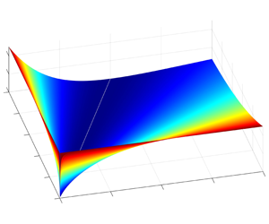
Three-dimensional plot of the relative multiplicative error  $\unicode[STIX]{x1D702}(\boldsymbol{p})$ as a function of pressure drop, calculated using the DW model and PM (white line denotes singularity of the relative index for zero pressure drop).

The relative error  $\unicode[STIX]{x1D702}(\boldsymbol{p})$ of the DW equation in relation to the PM for any pipeline geometry is shown in figure 2 as a two-dimensional plot, and in figure 3 as a three-dimensional graph. From these figures we can see that the DW equation underestimates pressure drop, and that for a large drop between (accordingly squared) inlet and outlet pressures the relative error $\unicode[STIX]{x1D702}(\boldsymbol{p})$ reaches about 25 % and follows a symmetric pattern.
One can observe ten levels of the error marked in figure 2, which lie in the areas between the two lines (under the appropriate sector angles to the white line). This chart should be interpreted as a strict dependence of the multiplicative error in relation to the inlet and outlet pressures. For example, to maintain a 2.5 % relative error, we must meet the following pressure condition:  $0.56<p_{i}/p_{o}<1.77$ (allowing a return transfer). Similarly, in order to keep the level of this error at 10 %, the following, a more relaxed limitation, should be observed: $0.27<p_{i}/p_{o}<3.73$.
4.2 Additive error
It would also be interesting to take a look at a more important quantity, from the engineering viewpoint, the additive DW error taken as the difference between the two models measured in given units (pascals or bars).
Having the absolute/true multiplicative error  $\unicode[STIX]{x1D705}(\boldsymbol{p})$ as (4.1), we can easily calculate the factor of (3.15), $\unicode[STIX]{x1D700}(\boldsymbol{p})=\unicode[STIX]{x1D705}(\boldsymbol{p})-1$, which reflects additive error and gives us at least the rate of the difference between the PM and DW model (in terms of the resulting pressure drop). The difference can be calculated as
 $$\begin{eqnarray}\unicode[STIX]{x1D700}(\boldsymbol{p})=\unicode[STIX]{x1D705}(\boldsymbol{p})-1=\frac{4}{3}\left(1-\frac{p_{i}p_{o}}{p_{i}^{2}+2p_{i}p_{o}+p_{o}^{2}}\right)-1=\frac{1}{3}-\frac{4p_{i}p_{o}}{3(p_{i}+p_{o})^{2}}.\end{eqnarray}$$
Eventually, we get the following final form of the additive error factor:
 $$\begin{eqnarray}\unicode[STIX]{x1D700}(\boldsymbol{p})=\frac{p_{i}-p_{o}}{3(p_{i}+p_{o})}.\end{eqnarray}$$
 Clearly, to obtain the true value of the pressure difference according to (3.15), the coefficient  $\unicode[STIX]{x1D700}(\boldsymbol{p})$ should be appropriately scaled using the physical parameters of the pipeline flow appearing in the expression $\unicode[STIX]{x1D706}(L/D)(\unicode[STIX]{x1D70C}u^{2}/2)$. As a result, the simple difference between the models is
 $$\begin{eqnarray}e(\boldsymbol{p})=\unicode[STIX]{x1D735}\boldsymbol{p}_{P\unicode[STIX]{x2202}}-\unicode[STIX]{x1D735}\boldsymbol{p}_{\unicode[STIX]{x2202}}=\unicode[STIX]{x1D706}\frac{L}{D}\frac{\unicode[STIX]{x1D70C}u^{2}}{2}\unicode[STIX]{x1D700}(\boldsymbol{p}).\end{eqnarray}$$
 Since  $u=q/\unicode[STIX]{x1D70C}S$ and the mass flow rate is given by (2.3), we obtain the following additive error:
 $$\begin{eqnarray}e(\boldsymbol{p})=\unicode[STIX]{x1D706}\frac{L}{D}\frac{\unicode[STIX]{x1D70C}DS^{2}(p_{i}^{2}-p_{o}^{2})}{\unicode[STIX]{x1D706}L\unicode[STIX]{x1D708}^{2}2S^{2}\unicode[STIX]{x1D70C}^{2}}\unicode[STIX]{x1D700}(\boldsymbol{p}),\end{eqnarray}$$
which after simplifications leads to
 $$\begin{eqnarray}e(\boldsymbol{p})=\frac{(p_{i}^{2}-p_{o}^{2})}{2\unicode[STIX]{x1D708}^{2}\unicode[STIX]{x1D70C}}\unicode[STIX]{x1D700}(\boldsymbol{p}).\end{eqnarray}$$
It should be noted that in the above error formula there are no pipe parameters (depending on the experiment) and that it only depends on the pressures and fluid density. Taking into account equation (3.5), we can further simplify (4.7) to its pure pressure function
 $$\begin{eqnarray}e(\boldsymbol{p})=\frac{(p_{i}^{2}-p_{o}^{2})}{2p}\unicode[STIX]{x1D700}(\boldsymbol{p}).\end{eqnarray}$$
 The substitution of  $p$ from (3.11) and $\unicode[STIX]{x1D700}(\boldsymbol{p})$ from (4.4) in the above form of the additive error leads to
 $$\begin{eqnarray}\displaystyle & \displaystyle e(\boldsymbol{p})=\frac{3}{2}\frac{p_{i}^{2}-p_{o}^{2}}{p_{i}^{3}-p_{o}^{3}}\frac{(p_{i}^{2}-p_{o}^{2})}{2}\frac{p_{i}-p_{o}}{3(p_{i}+p_{o})}, & \displaystyle\end{eqnarray}$$
 $$\begin{eqnarray}\displaystyle & \displaystyle e(\boldsymbol{p})=\frac{1}{4}\frac{(p_{i}^{2}-p_{o}^{2})^{2}}{(p_{i}-p_{o})(p_{i}^{2}+p_{i}p_{o}+p_{o}^{2})}\frac{p_{i}-p_{o}}{(p_{i}+p_{o})}, & \displaystyle\end{eqnarray}$$
 $$\begin{eqnarray}\displaystyle & \displaystyle e(\boldsymbol{p})=\frac{1}{4}\frac{(p_{i}-p_{o})(p_{i}^{2}-p_{o}^{2})}{(p_{i}^{2}+p_{i}p_{o}+p_{o}^{2})}. & \displaystyle\end{eqnarray}$$
 Thus, it can be seen that the additive error of the DW model is independent of the flow geometry (physics) factor  $\unicode[STIX]{x1D6F1}_{g}$ introduced in Kowalczuk & Tatara (Reference Kowalczuk and Tatara2018) as
 $$\begin{eqnarray}\unicode[STIX]{x1D6F1}_{g}=\sqrt{\frac{\unicode[STIX]{x1D706}L}{D}}.\end{eqnarray}$$
 It is important that only the generic (driving) pressures affect both the pressure drop and the additive error of the DW model. However, for example, the scale of the pipeline has no effect on this. In other words, for the same fluid in two different pipes, driven by identical inlet and outlet pressures, the DW error effect will be the same. The additive error  $e(\boldsymbol{p})$ is shown in figure 4 as a two-dimensional graph, and in figure 5 as a three-dimensional chart.
Additive error  $e(\boldsymbol{p})$ of the pressure drop calculated using the DW model.

Three-dimensional plot of the error  $e(\boldsymbol{p})$ of the DW equation determining the pressure drop.

Figure 4 is similar, although it represents a different measure and is somehow moved in relation to figure 2. It is instructive to say that for the additive difference, we cannot draw straight lines that provide a certain level of error, as was possible in figure 2. The three-dimensional chart in figure 5 shows that the additive error evolves smoothly under the influence of pressure drop variations, while the multiplicative error of figure 3 is characterized by abrupt changes, especially in the area of low pressures.
5 Experimental considerations
In order to practically justify the correctness of the presented results, an experimental study was carried out, including measurements of flow and pressure for known parameters of fluids and pipes. To preserve the impartiality of this study, instead of doing our own experiments, we used measurements available in the literature.
The problem with showing the consistency of our results is that the value of the friction factor is not precisely known, although the Moody diagram may be used to estimate it. Most often, this value is estimated in a way that compensates for modelling and measurement errors. Therefore, the friction factor may in practice deviate from its actual value (Billmann & Isermann Reference Billmann and Isermann1987).
Adiutori (Reference Adiutori2009) proposed to abandon the use of the friction factor and the Moody chart in known forms and provided a set of equations describing the flow and a transformed chart. In addition, in McGovern (Reference McGovern2011), the author cites Moody’s words that ‘it must be recognized that any high degree of accuracy in determining  $f$ is not to be expected’ (where $f$ is the friction factor, denoted here as $\unicode[STIX]{x1D706}$). On the other hand, in LDI systems the coefficient of friction is vital in determining the parameters of the leak and affects the accuracy of the results.
5.1 Friction factor estimation
Below are described four methods for estimating the friction factor using physical–mathematical relationships.
The first two methods are related to the compounds derived in this article, which require measurements of flow and pressure (inlet and outlet). Let us start with the solution (3.6) relative to  $\unicode[STIX]{x1D706}$:
 $$\begin{eqnarray}\unicode[STIX]{x1D706}=\frac{D}{L}\frac{p_{i}^{2}-p_{o}^{2}}{\unicode[STIX]{x1D70C}u^{2}p}.\end{eqnarray}$$
 In our experiment, in the above formula, the parameters are either fixed ( $D$,
$D$,  $L$ and $\unicode[STIX]{x1D70C}$) or measured ( $p_{i}$, $p_{o}$ and $u$), except the reference pressure $p$. Let us use $p$ appropriate for the approximate approach, which leads to the friction factor corresponding to the DW equation, which we denote as case ( $i$):
$i$):
 $$\begin{eqnarray}\unicode[STIX]{x1D706}_{\unicode[STIX]{x2202}}(\boldsymbol{p})=\frac{2D}{L}\frac{p_{i}^{2}-p_{o}^{2}}{\unicode[STIX]{x1D70C}u^{2}(p_{i}+p_{o})}=\frac{2D}{L}\frac{p_{i}-p_{o}}{\unicode[STIX]{x1D70C}u^{2}}.\end{eqnarray}$$
 Instead of using the approximate mean reference pressure, we can apply the precise value associated with the PM equation, which leads to  $\unicode[STIX]{x1D706}$ assigned to case ( $ii$):
 $$\begin{eqnarray}\unicode[STIX]{x1D706}_{P\unicode[STIX]{x2202}}(\boldsymbol{p})=\frac{2D}{L}\frac{p_{i}-p_{o}}{\unicode[STIX]{x1D70C}u^{2}\unicode[STIX]{x1D705}(\boldsymbol{p})}.\end{eqnarray}$$
 According to the above discussion on problems with the friction factor (in the above two cases ( $i$) and ( $ii$) also), in practice such a friction factor is applied that matches both the measurement data and the adopted model. This can directly lead to a biased estimation of the flow rate (used for volume balancing or parity equations) in the event of a leak. Therefore, in sensitive cases it is more rational to use the exact Colebrook relationship (White Reference White1986), which binds the coefficient of friction:
 $$\begin{eqnarray}\frac{1}{\sqrt{\unicode[STIX]{x1D706}}}=-2\log _{10}\left(\frac{\unicode[STIX]{x1D716}}{3.7D}+\frac{2.51}{Re\sqrt{\unicode[STIX]{x1D706}}}\right),\end{eqnarray}$$
 where  $\unicode[STIX]{x1D716}$ is the roughness height (m) and $Re$ is the dimensionless Reynolds number defined as
 $$\begin{eqnarray}Re=\frac{\unicode[STIX]{x1D70C}Du}{\unicode[STIX]{x1D707}}=\frac{Dq}{S\unicode[STIX]{x1D707}},\end{eqnarray}$$
 in which  $\unicode[STIX]{x1D707}$ is the dynamic viscosity of the fluid (Pa s).
The concept of friction factor is very important and is therefore widely used in practice. Over the years, many explicit patterns (Brkić Reference Brkić2011) approximating the implicit formula (5.4) have been proposed. Nevertheless, a sufficiently accurate and explicit formula has not been developed. Therefore, the next part of this work presents such a solution.
To solve the implicit equation (5.4) for the friction factor, first let us put the Reynolds number (5.5) into (5.4):
 $$\begin{eqnarray}\frac{1}{\sqrt{\unicode[STIX]{x1D706}}}=-2\log _{10}\left(\frac{\unicode[STIX]{x1D716}}{3.7D}+\frac{2.51S\unicode[STIX]{x1D707}}{Dq\sqrt{\unicode[STIX]{x1D706}}}\right).\end{eqnarray}$$
 Now, using  $u=q/\unicode[STIX]{x1D70C}S$ in (5.1), we can determine the mass flow as
 $$\begin{eqnarray}q=\sqrt{\frac{\unicode[STIX]{x1D70C}S^{2}D}{L}\frac{p_{i}^{2}-p_{o}^{2}}{\unicode[STIX]{x1D706}p}}\end{eqnarray}$$
and consequently, inserting the above in (5.6), we get the following result:
 $$\begin{eqnarray}\frac{1}{\sqrt{\unicode[STIX]{x1D706}}}=-2\log _{10}\left(\frac{\unicode[STIX]{x1D716}}{3.7D}+\frac{2.51S\unicode[STIX]{x1D707}\sqrt{Lp}}{D\sqrt{\unicode[STIX]{x1D70C}S^{2}D(p_{i}^{2}-p_{o}^{2})}}\right),\end{eqnarray}$$
 which is explicit and independent of  $q$. Thus, only the pressure measurements and the pipe and medium parameters are needed to determine the friction factor (and iteration is not required). Although two parameters, the roughness and viscosity of the fluid, are quite difficult to accurately estimate, this formula should be considered to be more objective and closer to reality. Equation (5.8) can be further converted to yield an explicit form of the friction factor:
 $$\begin{eqnarray}\unicode[STIX]{x1D706}=\left(-2\log _{10}\left[\frac{\unicode[STIX]{x1D716}}{3.7D}+\frac{2.51\unicode[STIX]{x1D707}\sqrt{Lp}}{\sqrt{\unicode[STIX]{x1D70C}D^{3}(p_{i}^{2}-p_{o}^{2})}}\right]\right)^{-2}.\end{eqnarray}$$
 On the basis of (5.9) (compare model (5.1)) we can derive two other formulas for  $\unicode[STIX]{x1D706}$ using the two previously applied reference pressures.
Taking the approximate equation we get another standard case ( $iii$):
 $$\begin{eqnarray}\unicode[STIX]{x1D706}_{C\unicode[STIX]{x2202}}(\boldsymbol{p})=\left(-2\log _{10}\left[\frac{\unicode[STIX]{x1D716}}{3.7D}+\frac{2.51\unicode[STIX]{x1D707}\sqrt{L}}{\sqrt{2\unicode[STIX]{x1D70C}D^{3}(p_{i}-p_{o})}}\right]\right)^{-2},\end{eqnarray}$$
 while the precise reference pressure leads to the following improved case ( $iv$):
 $$\begin{eqnarray}\unicode[STIX]{x1D706}_{CP\unicode[STIX]{x2202}}(\boldsymbol{p})=\left(-2\log _{10}\left[\frac{\unicode[STIX]{x1D716}}{3.7D}+\frac{2.51\unicode[STIX]{x1D707}\sqrt{L\unicode[STIX]{x1D705}(\boldsymbol{p})}}{\sqrt{2\unicode[STIX]{x1D70C}D^{3}(p_{i}-p_{o})}}\right]\right)^{-2}.\end{eqnarray}$$
 The two estimates (5.10) and (5.11), referring to DW and PM, can be used to determine the flow  $q$, but with the limitation characteristic of the Colebrook formula that $Re>4000$. Clearly, in both solutions one can use either the dynamic viscosity $\unicode[STIX]{x1D707}$ or the kinematic viscosity $v=\unicode[STIX]{x1D707}/\unicode[STIX]{x1D70C}$.
It is worth noting that the presented methodology can be applied even to other implicit formulas derived/invented to calculate the coefficient of friction. However, it should be remembered that such a relationship should have one of the following three equivalent forms:  $\unicode[STIX]{x1D706}=f(u\sqrt{\unicode[STIX]{x1D706}})$, $\unicode[STIX]{x1D706}=f(q\sqrt{\unicode[STIX]{x1D706}})$ or $\unicode[STIX]{x1D706}=f(Re\sqrt{\unicode[STIX]{x1D706}})$.
5.2 Ratings dependent on friction
In LDI systems based on mass or volume balancing, the flow rate resulting from the applied model is compared to the appropriate measured variable. This allows the generation of residual signals that provide symptoms and other information necessary to determine the size of a leak. In view of this, let us now consider the flow rate estimates resulting from the DW and PM approaches.
Note that in all four cases ( $i$)–( $iv$), represented by (5.2), (5.3), (5.10) and (5.11), the friction factor $\unicode[STIX]{x1D706}$ is a function of the inlet and outlet pressures that may vary (e.g. due to leakage). Therefore, more accurate estimates of $\unicode[STIX]{x1D706}$ can improve the results of diagnostic procedures.
Let us introduce a new instrumental variable  $\unicode[STIX]{x1D709}$ describing the pressure ratio (type of relative excitation) for the DW model first:
 $$\begin{eqnarray}\unicode[STIX]{x1D709}=\frac{p_{i}}{p_{o}}.\end{eqnarray}$$
 Note that  $\unicode[STIX]{x1D709}=1$ means that $p_{o}=p_{i}$, and $\unicode[STIX]{x1D709}\rightarrow \infty$ denotes situation where $p_{i}\rightarrow \infty$ or $p_{o}\rightarrow 0$. As a consequence, all possible situations are included in the range $\unicode[STIX]{x1D709}\in [1,\infty )$. With this notation in mind, let us now analyse the impact of the calculation method on the estimated flow rate $u$.
$u$.
On the basis of the DW equation (3.8) we obtain
 $$\begin{eqnarray}\displaystyle & \displaystyle p_{i}-p_{o}=\unicode[STIX]{x1D706}\frac{L}{D}\frac{\unicode[STIX]{x1D70C}u^{2}}{2}, & \displaystyle\end{eqnarray}$$
 $$\begin{eqnarray}\displaystyle & \displaystyle u_{\unicode[STIX]{x2202}}=u_{\unicode[STIX]{x2202}}(\boldsymbol{p})=\sqrt{\frac{2(p_{i}-p_{o})D}{\unicode[STIX]{x1D706}L\unicode[STIX]{x1D70C}}}. & \displaystyle\end{eqnarray}$$
To show the precise flow rate computation, let us take (3.12)
 $$\begin{eqnarray}p_{i}-p_{o}=\unicode[STIX]{x1D706}\frac{L}{D}\unicode[STIX]{x1D70C}u^{2}\frac{2}{3}\frac{(p_{i}^{2}+p_{i}p_{o}+p_{o}^{2})}{(p_{i}+p_{o})^{2}}\end{eqnarray}$$
 and present it as a function of the pressure ratio  $\unicode[STIX]{x1D709}$ from (5.12):
 $$\begin{eqnarray}p_{i}-p_{0}=\unicode[STIX]{x1D706}\frac{L}{D}\frac{\unicode[STIX]{x1D70C}u^{2}}{2}\frac{4}{3}\frac{(\unicode[STIX]{x1D709}^{2}+\unicode[STIX]{x1D709}+1)}{(\unicode[STIX]{x1D709}+1)^{2}}=\unicode[STIX]{x1D706}\frac{L}{D}\frac{\unicode[STIX]{x1D70C}u^{2}}{2}\unicode[STIX]{x1D705}(\unicode[STIX]{x1D709}),\end{eqnarray}$$
 where  $\unicode[STIX]{x1D705}(\unicode[STIX]{x1D709})={\textstyle \frac{4}{3}}(1-\unicode[STIX]{x1D709}/(\unicode[STIX]{x1D709}+1)^{2})_{\mid _{\unicode[STIX]{x1D709}=p_{i}/p_{o}}}=\unicode[STIX]{x1D705}(\boldsymbol{p})$ (with a little symbol abuse). This ultimately leads to a precise pressure-dependent estimation of the flow rate as
 $$\begin{eqnarray}u_{P\unicode[STIX]{x2202}}(\boldsymbol{p})=u_{P\unicode[STIX]{x2202}}(\unicode[STIX]{x1D709})=\sqrt{\frac{2(p_{i}-p_{o})D}{\unicode[STIX]{x1D706}L\unicode[STIX]{x1D70C}}}\sqrt{\frac{1}{\unicode[STIX]{x1D705}(\unicode[STIX]{x1D709})}}=\frac{u_{\unicode[STIX]{x2202}}}{\sqrt{\unicode[STIX]{x1D705}(\unicode[STIX]{x1D709})}},\end{eqnarray}$$
 and  $\unicode[STIX]{x1D710}_{P}$ as a ratio of the above two velocities can be considered as another pressure-dependent scaling coefficient or a necessary multiplicative corrector in relation to the DW computation of (5.14):
 $$\begin{eqnarray}\unicode[STIX]{x1D710}_{P}=\frac{u_{P\unicode[STIX]{x2202}}}{u_{\unicode[STIX]{x2202}}}=\frac{1}{\sqrt{\unicode[STIX]{x1D705}(\unicode[STIX]{x1D709})}}.\end{eqnarray}$$
 The flow rate corrector  $\unicode[STIX]{x1D710}_{P}(\unicode[STIX]{x1D709})$ is depicted in figure 6.
Plot of  $\unicode[STIX]{x1D710}_{P}(\unicode[STIX]{x1D709})$, the ratio of PM and DW estimates of the flow rate as a function of the relative pressure $\unicode[STIX]{x1D709}$. The dashed line indicates the asymptote at the value $\unicode[STIX]{x1D710}_{P}=\sqrt{{\textstyle \frac{3}{4}}}$ for $\unicode[STIX]{x1D709}\rightarrow \infty$.

5.3 Experimental study
In order to support our previous considerations with practical results, we will show the application of the discussed methods to experimental data. It is worth noticing that both experiments consist of two parts: (i) stationary flow without leakage and (ii) stationary flow with leakage. There is a short transient between these two phases, which is, however, irrelevant from the point of view of system (diagnostic) applications.
5.3.1 Experiment 1
First, let us consider the experimental data from the work of Espinoza-Moreno, Begovich & Sanchez-Torres (Reference Espinoza-Moreno, Begovich and Sanchez-Torres2014) (retrieved from a digital copy of the paper; the data do not have to be fully consistent). The experiment was carried out on a pipeline with the characteristics of  $D=0.06271~(\text{m})$ and $L=88.28~(\text{m})$, while the pressure head and volumetric flow rates were measured at the inlet and outlet of the pipe. In addition, the authors specified the other parameters as $\unicode[STIX]{x1D70C}=993.054~(\text{kg}~\text{m}^{-3})$, $\unicode[STIX]{x1D716}=7\times 10^{-6}~(\text{m})$, $v=6.8817\times 10^{-7}(\text{m}^{2}~\text{s}^{-1})$ and $T=37.72~(\text{}^{\circ }\text{C})$. The Reynolds number for this experiment can be calculated from (5.5); it lies in the range $2.44\times 10^{5}{-}2.53\times 10^{5}$ with relative pipe roughness $\unicode[STIX]{x1D716}/D=1.12\times 10^{-4}$, which indicates that the flow is turbulent.
For our analysis, we need to convert the pressure head  $h$ to the pressure $p=\unicode[STIX]{x1D70C}gh$, and the volume flow $V$ to the mass flow rate according to $q=\unicode[STIX]{x1D70C}V$. The converted measurement data are shown in figures 7 and 8. Note that the measurements contain also the symptoms of a leak occurring at time $t_{L}\approx 30~(\text{s})$, which is not necessary in this analysis, but shows the important properties of our estimator.
Measurements of the inlet and outlet mass flow rates for experiment 1.

Measurement of inlet and outlet pressures for experiment 1 with reference pressures calculated using PM and DW (note that the model difference is more visible than in figure 1).

As a consequence of what can be seen in figures 2, 3, 4 and 5, this experiment (with  $\unicode[STIX]{x1D709}={\textstyle \frac{1.7}{0.85}}=2$), although placed in close proximity to the origins of the pressure plane in figure 1, results in a quantitative difference between the two reference pressures (DW and PM), as shown in figure 8.

Now we can simulate the use of recorded measurements in accordance with formulas (5.2)–(5.3) and (5.10)–(5.11) and estimation of the corresponding values of the friction factor. The obtained run-time results are presented in figure 9.
We can observe that the two friction factors estimated using the DW and PM approaches are realistically noisy and clearly distant from each other. Whereas in the sense of the friction factor, the values estimated using the Colebrook approach are closer to each other. Moreover, the obtained trajectories of  $\unicode[STIX]{x1D706}$ are quite smooth, as if they were low-pass filtered. Note that for the initial, faultless period in this experiment, the presumed true value resulting from Colebrook calculations lies between the approximate DW and PM estimates. What is very important is that the Colebrook estimates practically do not change after the leak occurs (which also indicates the rationality of Colebrook), while a significant change (of the order of 2 %) in the value of $\unicode[STIX]{x1D706}$ is obtained by means of the approximate approaches (DW and PM).
According to (5.3), with  $\unicode[STIX]{x1D705}(\unicode[STIX]{x1D709})$ as the factor of proportionality, the DW friction coefficient is greater than (proportional to) the PM friction coefficient:
 $$\begin{eqnarray}\unicode[STIX]{x1D706}_{\unicode[STIX]{x2202}}=\unicode[STIX]{x1D706}_{P\unicode[STIX]{x2202}}\;\unicode[STIX]{x1D705}(\unicode[STIX]{x1D709}).\end{eqnarray}$$
 What is opposed to the above (and to some extent surprising) is that, according to (5.11), the Colebrook PM friction coefficient is greater than the Colebrook DW friction coefficient, with some function of  $\unicode[STIX]{x1D705}(\unicode[STIX]{x1D709})$ as a proportionality factor:
 $$\begin{eqnarray}\unicode[STIX]{x1D706}_{CP\unicode[STIX]{x2202}}(\boldsymbol{p})=\unicode[STIX]{x1D706}_{C\unicode[STIX]{x2202}}\;f_{C}(\boldsymbol{p}),\end{eqnarray}$$
 where  $f_{C}(\boldsymbol{p})$ is a nonlinear (Colebrook) proportionality function resulting from (5.11).
5.3.2 Experiment 2
To provide more practical results, a different set of experimental data of recorded pressure and flow-rate measurements shown in figures 10 and 11 were taken from Torres et al. (Reference Torres, Besancon, Navarro, Begovich and Georges2011), and the technical details of the pipeline were taken from Garcia, Leon & Begovich (Reference Garcia, Leon and Begovich2009). Consequently, the following parameterization was used:  $D=0.0635~(\text{m})$, $L=85~(\text{m})$, $\unicode[STIX]{x1D70C}=1000~(\text{kg}~\text{m}^{-3})$, $\unicode[STIX]{x1D716}=7\times 10^{-6}~(\text{m})$. The resulting estimation of the friction factor using the four methods is shown in figure 12.
There was some uncertainty associated with the kinematic viscosity value, which in Garcia et al. (Reference Garcia, Leon and Begovich2009) is described as  $v=1.02\times 10^{-6}~(\text{m}^{2}~\text{s}^{-1})$, while in Navarro et al. (Reference Navarro, Begovich, Sánchez and Besancon2017) this value is given as $v=2\times 10^{-6}~(\text{m}^{2}~\text{s}^{-1})$ for apparently the same pipe. Thus, because the temperature of the experiment is unknown, and viscosity can not be determined unambiguously, the possible estimation error is depicted in the graph (figure 12) as a shaded zone (band). For better reference and visualization, the higher viscosity value was used in the Colebrook estimates. In this experiment, the Reynolds number was recalculated using (5.5). The range of this parameter was $4.03\times 10^{4}{-}8.55\times 10^{5}$ at relative pipe roughness $\unicode[STIX]{x1D716}/D=1.1\times 10^{-4}$, which again means turbulent flow. The Reynolds number distribution, in this case, results from the discussed uncertainty of kinematic viscosity.
Measurements of the inlet and outlet mass flow rates for experiment 2.

Measurements of inlet and outlet pressures for experiment 2 (reference pressures calculated using PM and DW are also indicated).


Again, we observe that the friction factors obtained from the Colebrook estimations change less than the other two, that is, respond less to leakage ( $t_{L}\approx 130~\text{s}$). Note that in the non-leakage case, the friction assessment resulting from the exact model (PM) appears to be closer to the supposed real value than that obtained from DW. Note that here the lower boundary of the Colebrook-estimated friction coefficient is around 0.019, while in Garcia et al. (Reference Garcia, Leon and Begovich2009) the authors assume $\unicode[STIX]{x1D706}=0.0187$ as the actual value.
5.4 Conclusions from the presented experiments
We have shown four methods for determining the coefficient of friction: two of them (DW and PM) match this value to measured data, while the other two (related to the Colebrook equation) are a combination of the generic Colebrook equation and the flow steady-state equation. In this case, the difference in the estimated flow velocity resulting from the application of the two analysed fundamental approaches (PM and DW) has been determined.
We applied the four calculation models (estimations) for the friction factor in relation to two different sets of experimental data. The relationship between the resulting estimates of  $\unicode[STIX]{x1D706}$ has been discussed, showing the advantages of using the Colebrook approach.
Relevant values of the Reynolds number and relative pipe roughness, indicating turbulent behaviour, were provided for both experiments.
Analysis of figures 9 and 12 leads to the conclusion that estimates based on Colebrook (5.10) and (5.11) are more robust to the technical parameters of the pipe and pressure changes, including those resulting from a leak. It is also important that the obtained estimates are characterized by a high degree of smoothing (reminiscent of low-pass filtration), resulting from logarithm and the inverse of the square root.
The proposed Colebrook-based estimation methods are therefore more robust to faults than the simple DW or PM approaches. However, it should be remembered that they require better knowledge of the process (additional parameters are required: roughness  $\unicode[STIX]{x1D716}$ and viscosity $v$). We have also shown that with the simple DW and PM estimates of the friction factor, DW overestimates the value of $\unicode[STIX]{x1D706}$, whereas on the basis of the Colebrook equation, the DW approach underestimates $\unicode[STIX]{x1D706}$.
We can therefore conclude that the PM method can be effectively used instead of the DW method to more accurately represent the flow and pressure relationships. However, there is a problem with the coefficient of friction, which is usually unreliable and is rather used to mask model uncertainty and modelling errors.
The kappa function  $\unicode[STIX]{x1D705}(\unicode[STIX]{x1D709})$, which is a pressure-dependent function and is the basis of the analysis used in this work, represents the multiplicative pressure corrector (4.1) of the original DW equation of (3.8) and plays several functional roles in defining multiplicative and additive errors (3.14) and (3.16), estimating the friction factor (5.2) and (5.11) or flow rate (5.17), based on the associated flow-rate corrector $\unicode[STIX]{x1D710}_{P}$ of (5.18).
A small difference between the ratings of the reference pressure in figures 9 and 12 can be explained by the course of the kappa function shown in figure 13, which reflects the run of the kappa function as well as its enlarged initial part.
Generic function  $\unicode[STIX]{x1D705}(\unicode[STIX]{x1D709})$ along with the parameters of the two experiments.

6 Conclusion
This article presents a steady-state isothermal flow model for transmission pipelines calculated in two ways. The first approach of an approximate nature led us to the well-known DW equation. By using a precise approach based on the appropriate calculation of the mean pressure in the pipe, we derived a precise steady-state model (PM).
We also presented two, multiplicative and additive ways of assessing the differences between the considered models. We showed that for higher pressure differences the DW equation underestimates the pressure drop. Moreover, we have proved that the error of the DW model is independent of the geometric factor of the pipe and that only the pressure difference affects this error (i.e. the difference between the estimates of the model). Obviously, as usual in such cases, one should remember the assumptions regarding the incompressibility of the fluid and the isothermal nature of the flow process.
We note that the assumption in our considerations that the coefficient of friction is constant can be practically solved by online estimation. In consequence, any possible discrepancies in its constancy can be compensated on an ongoing basis by using the estimated coefficient of friction (which will then also represent a certain overall fit factor of the model).
Since the concept of the friction factor is extremely important and widely used in practice, many explicit formulas have been proposed that approximate the implicit formula of Colebrook (a few of which are those of Swamee and Jain, Haaland, Brkić, Romeo, Rao and Buzzelli). However, to date, no sufficiently accurate and explicit formula has been developed. Note that our result is just of this type. We should also note that our methodology for solving the problem of implicitness of the Colebrook pattern can also be applied to other analytic forms of the friction factor relationships (having, however, one of the following equivalent forms:  $\unicode[STIX]{x1D706}=f(u\sqrt{\unicode[STIX]{x1D706}})$, $\unicode[STIX]{x1D706}=f(q\sqrt{\unicode[STIX]{x1D706}})$ or $\unicode[STIX]{x1D706}=f(Re\sqrt{\unicode[STIX]{x1D706}})$).
Four methods of estimating the friction coefficient were presented in support of our considerations. The effect of the pressure difference on the estimated mean flow velocity was assessed. Two sets of experimental data were used to show the suitability of our proposals in various applications. Certainly, the possibility of using the procedure for estimating the coefficient of friction should be further investigated.
It is worth noting that the derivation of a constant flow does not include any calculations in the discrete domain (neither in space nor in time), and is based only on the assumption that time derivatives of pressure and flow reach zero values. Due to the above, the solutions obtained are completely unambiguous and we can say that they describe the actual steady state (within the accepted theory).
Note also that for gases,  $\unicode[STIX]{x1D708}$ can be treated as the velocity of sound and roughly considered a constant parameter. In the case of liquids, this assumption is generally not correct, as indicated in the discussion of this phenomenon in appendix A.
The obtained results of the steady-state flow process model can be used, for example: (i) for online estimation of the coefficient of friction; (ii) in the pipeline design process, when the unknown parameters are adapted to the required flow assumptions; and (iii) in model-based LDI systems.
It is also worth noting that the presented experiments consisted of two parts: (i) stationary flow without leakage and (ii) stationary flow with leakage. Of course, between these two phases, there is a short transient state, which, however, does not matter from the point of view of the diagnostic system application.
Declaration of interests
The authors report no conflict of interest.
Appendix A. Note on sound speed and bulk modulus
As mentioned earlier, under some circumstances the factor  $\unicode[STIX]{x1D708}$ given in (3.5) can be related to the speed of sound in fluids. Note, however, that this approximate interpretation, applied by Isermann (Reference Isermann1982) (see also Isermann (Reference Isermann1984) and White (Reference White1986)) when deriving the base model (2.1)–(2.2), is only suitable for ideal incompressible gas flows.
In general, using the Newton–Laplace formula (Wang et al. Reference Wang, Nilsson, Yang and Petit2017) with the bulk modulus  $K$, the velocity of sound in fluids can be given as
 $$\begin{eqnarray}\unicode[STIX]{x1D708}=\sqrt{\frac{K}{\unicode[STIX]{x1D70C}}}.\end{eqnarray}$$
 For all fluids the isentropic bulk modulus  $K$ can be defined as (White Reference White1986)
 $$\begin{eqnarray}K=\unicode[STIX]{x1D70C}\frac{\unicode[STIX]{x2202}p}{\unicode[STIX]{x2202}\unicode[STIX]{x1D70C}},\end{eqnarray}$$
which used in (A 1) leads to
 $$\begin{eqnarray}\unicode[STIX]{x1D708}=\sqrt{\frac{\unicode[STIX]{x2202}p}{\unicode[STIX]{x2202}\unicode[STIX]{x1D70C}}}.\end{eqnarray}$$
 To simplify the discussion below, let us focus on the expression  $\unicode[STIX]{x2202}p/\unicode[STIX]{x2202}\unicode[STIX]{x1D70C}$, separately for gases and liquids.
A.1 Gaseous media
At high temperatures and low pressures, all gases comply with the perfect gas law (White Reference White1986), using the universal gas constant  $R$:
$R$:
 $$\begin{eqnarray}p=\unicode[STIX]{x1D70C}RT.\end{eqnarray}$$
 Assuming that  $R$ and $T$ are approximately constant and independent of density and pressure, we can determine the derivative
 $$\begin{eqnarray}\frac{\unicode[STIX]{x2202}p}{\unicode[STIX]{x2202}\unicode[STIX]{x1D70C}}\approx RT.\end{eqnarray}$$
 According to (A 4),  $RT=p/\unicode[STIX]{x1D70C}$, and we can conclude that the following approximation applies: $\unicode[STIX]{x2202}p/\unicode[STIX]{x2202}\unicode[STIX]{x1D70C}\approx p/\unicode[STIX]{x1D70C}$. It can thus be seen that for gases at low pressure and high temperatures the following approximate rule applies:
 $$\begin{eqnarray}K\approx p.\end{eqnarray}$$
 Another way to justify approximation (A 6) is based on the definition of the bulk modulus using a heat capacity factor  $\unicode[STIX]{x1D6FE}$:
 $$\begin{eqnarray}K=\unicode[STIX]{x1D6FE}p.\end{eqnarray}$$
 For perfect gases in isothermal conditions  $\unicode[STIX]{x1D6FE}=1$, whereas in general $\unicode[STIX]{x1D6FE}$ is greater than 1. What is more, the bulk modulus used in (A 1) to calculate the ‘sound velocity’ occurs under the square root function, so the $\unicode[STIX]{x1D6FE}\cong 1$ effect is additionally suppressed, which means we can write the following:
 $$\begin{eqnarray}\unicode[STIX]{x1D708}=\sqrt{\frac{\unicode[STIX]{x2202}p}{\unicode[STIX]{x2202}\unicode[STIX]{x1D70C}}}=\sqrt{\frac{K}{\unicode[STIX]{x1D70C}}}\approx \sqrt{\frac{p}{\unicode[STIX]{x1D70C}}},\end{eqnarray}$$
which also leads to the previously determined approximation
 $$\begin{eqnarray}K\approx p.\end{eqnarray}$$
 Both methods, in the case of the isothermal and incompressible flow of gases, lead to the speed of sound (3.5) in gaseous media. In general, however, the coefficient  $\unicode[STIX]{x1D708}$ can only be treated as a surrogate of sound speed; it is expressed in units of speed, but should not be identified with the speed of sound in fluids.
Note that the approximate equality  $p/\unicode[STIX]{x1D70C}=\unicode[STIX]{x2202}p/\unicode[STIX]{x2202}\unicode[STIX]{x1D70C}$ is a special case of the Clairaut equation, with the linear solution $p(\unicode[STIX]{x1D70C})=C\unicode[STIX]{x1D70C}$ for the constant $C=RT$ (see (A 4) or White (Reference White1986)), which can be referred to a gas phase characteristic of relatively low pressure and relatively high temperature (relative to a critical point). Then it is certain that the pressure changes linearly with the density, $p/\unicode[STIX]{x1D70C}=C$, and also $\unicode[STIX]{x2202}p/\unicode[STIX]{x2202}\unicode[STIX]{x1D70C}=C$. In addition, in the general case of monotonic relationships in a vicinity of zero, the high pressure-to-density ratio ( $p/\unicode[STIX]{x1D70C}$) also produces a large derivative there. It is instructive to see that at low pressure in the range of 1–100 bar the ratio $p/\unicode[STIX]{x1D70C}$ is about $10^{5}{-}10^{7}~(\text{m}^{2}~\text{s}^{-2})$, while $\unicode[STIX]{x2202}p/\unicode[STIX]{x2202}\unicode[STIX]{x1D70C}$ (square of actual sound velocity) is also in a similar range of $10^{4}{-}10^{6}~(\text{m}^{2}~\text{s}^{-2})$.
A.2 Liquid media
The above approximation ( $\unicode[STIX]{x2202}p/\unicode[STIX]{x2202}\unicode[STIX]{x1D70C}\approx p/\unicode[STIX]{x1D70C}$, and therefore $K\approx p$) can be used for incompressible fluid flows only at very high pressures (from 1000 to 100 000 (bar), depending on the fluid). In practice, therefore, we cannot use it for liquids. This statement can easily be justified by the fact that bulk moduli for liquids have the same order of magnitude $(10^{8}{-}10^{10}~(\text{Pa}))$. Therefore, for the above approximation ( $K\approx p$) to be met, such very large pressures would be necessary.
It is also worth noting that in the case of liquids we do not have such a high pressure-to-density ratio  $p/\unicode[STIX]{x1D70C}$ (it roughly reaches values in the range of $10^{2}{-}10^{4}~(\text{m}^{2}~\text{s}^{-2})$), while $\unicode[STIX]{x2202}p/\unicode[STIX]{x2202}\unicode[STIX]{x1D70C}$ (which should not be identified with the square of sound speed) has much higher values (in the range of $10^{6}{-}10^{7}~(\text{m}^{2}~\text{s}^{-2})$). This means that in the case of liquids both quantities are definitely different (and not comparable).
Note that this consideration does not invalidate the correctness of the underlying discussion and pressure ranges used in this work, because the factor  $\unicode[STIX]{x1D708}$ shown in (3.5) does not need to be related to the speed of sound.
Appendix B. Note on compressibility
In general, the assumption of incompressibility of the analysed experimental case is associated with a practical limitation imposed on the flow velocity, for instance. According to White (Reference White1986), the flow is considered incompressible if the Mach number is less than 0.3. Note that this boundary is not the exact point at which fluid behaviour drastically changes its nature, but rather a rational, practice-based indicator that allows one to distinguish when to use the appropriate model (this value is also approximate: for example Durst (Reference Durst2008) sets it to 0.2). Therefore, one has to take into account that there are cases when an incompressible fluid appears to be weakly compressible.
It is interesting to compare the model (3.6) in the following rearranged form:
 $$\begin{eqnarray}\unicode[STIX]{x1D70C}^{2}u^{2}=\unicode[STIX]{x1D70C}\frac{p_{i}^{2}-p_{o}^{2}}{p\unicode[STIX]{x1D706}{\displaystyle \frac{L}{D}}}\end{eqnarray}$$
with the isothermal stationary compressible flow equation (White Reference White1986):
 $$\begin{eqnarray}G^{2}=\frac{\unicode[STIX]{x1D70C}(p_{i}^{2}-p_{o}^{2})}{p\left(\unicode[STIX]{x1D706}{\displaystyle \frac{L}{D}}+2\ln (\unicode[STIX]{x1D709})\right)},\end{eqnarray}$$
 where  $G=\unicode[STIX]{x1D70C}u$. The difference between these two equations is in the expression $2\ln (\unicode[STIX]{x1D709})$. For $\unicode[STIX]{x1D709}$ located in a small vicinity of 1, the logarithm is close to 0. On the other hand, as the pressure factor increases, this term becomes more significant (in relation to $\unicode[STIX]{x1D706}(L/D)$); it thus cannot be ignored, and one should consider compressibility effects. Furthermore, when we use the Taylor series expansion for this logarithm expression, whose centre is $\unicode[STIX]{x1D709}=1$, i.e. $2\ln (\unicode[STIX]{x1D709})\approx (\unicode[STIX]{x1D709}-1)+R(\unicode[STIX]{x1D709})$, after cutting the remainder $R(.)$, we get an easy-to-analyse form:
 $$\begin{eqnarray}G^{2}=\frac{\unicode[STIX]{x1D70C}(p_{i}^{2}-p_{o}^{2})}{p\left(\unicode[STIX]{x1D706}{\displaystyle \frac{L}{D}}+2(\unicode[STIX]{x1D709}-1)\right)}.\end{eqnarray}$$
To sum up: when  $\unicode[STIX]{x1D709}$ approaches 1, this expression can be omitted, but as $\unicode[STIX]{x1D709}$ increases, it becomes significant, and the flow should be considered compressible.
Note that figures 1–6 relate to various fluids, but not without restrictions. They are, for example, theoretical in the sense that not all of their scope (domain) is appropriate for the incompressible flow under consideration.
To get a quantitative view on the issue of the limiting pressure ratio differentiating incompressible from compressible flow, let us consider two cases of pipelines, for gas and liquid. To see the difference, in both cases the average velocity will be calculated using both equations, for the incompressible fluid (3.12), with the mean pressure calculated using the PM, and the compressible fluid (B 2), respectively.
Certainly, these calculations are rough, and therefore the results are also approximate. In both cases, the mean pressure will be calculated using the integral average (3.11). For simplicity, it is assumed that there is atmospheric pressure at the outlet:  $p_{o}=1$ bar.
B.1 Gaseous media
For gaseous media, we use the following parameters related to the flow of compressed natural gas through a relatively short pipe:  $\unicode[STIX]{x1D70C}=0.8~(\text{kg}~\text{m}^{-3})$, $L=100~(\text{m})$, $D=0.2~(\text{m})$, $\unicode[STIX]{x1D706}=0.03$, $\unicode[STIX]{x1D708}=300~(\text{m}~\text{s}^{-1})$ (sound speed is only used here to calculate the Mach number). In this experimental setting, the Mach number is 0.3 at $\unicode[STIX]{x1D709}=p_{i}/p_{o}=2.16$, when using the compressible flow equation, while the incompressible formula results in $\unicode[STIX]{x1D709}=2.07$.
For the same fluid we can simulate flow through a long pipe characterized by the following parameters:  $L=100~(\text{km})$, $D=1~(\text{m})$, $\unicode[STIX]{x1D706}=0.03$. In this experimental setting, the Mach number equal to 0.3 is obtained at $\unicode[STIX]{x1D709}=p_{i}/p_{o}=132.6$ based on compressible flow, and at $\unicode[STIX]{x1D709}=132.1$ while using incompressible flow. It is worth noting that the above simple analysis does not take into account the change in density or speed of sound due to the increase in pressure, and that the obtained critical pressure ratios are similarly high.
B.2 Liquid media
The above examples of long and short pipes can also be converted for liquid media.
Let us first consider the example of a short pipe for the transport of liquefied natural gas characterized by the following parameters:  $\unicode[STIX]{x1D70C}=468~(\text{kg}~\text{m}^{-3})$, $L=100~(\text{m})$, $D=0.2~(\text{m})$, $\unicode[STIX]{x1D706}=0.03$, $\unicode[STIX]{x1D708}=920~(\text{m}~\text{s}^{-1})$ (again, the speed of sound is used here only to calculate the Mach number). For this experimental setting, the critical pressure ratio causing the Mach number to be 0.3 is enormous: $\unicode[STIX]{x1D709}=3568$ and $\unicode[STIX]{x1D709}=3575$ for incompressible and compressible flows, respectively.
In the case of a long pipe with parameters  $L=100~(\text{km})$, $D=1~(\text{m})$, $\unicode[STIX]{x1D706}=0.03$, the Mach number is 0.3 only at the unusually huge $\unicode[STIX]{x1D709}\cong 700\,000$ for both equations (the difference between the corresponding high ratios is practically insignificant).
The above cases show that for liquids or long pipelines, the pressure ratio would have to be very high to fall within the compressibility range. In turn, for gases and short pipes, the flow becomes compressible at a relatively low pressure ratio. This analysis is approximate, but shows the difference between liquid and gaseous media in terms of compressibility. It can also be seen that the difference between the cases of long and short pipes is due to the factor  $\unicode[STIX]{x1D706}(L/D)$, which is one of the main determinants of whether a pipe can be considered long or not. Another factor affecting critical $\unicode[STIX]{x1D709}$ is the ratio of density to mean pressure.


 Open access