





1. Introduction
When a flow passes over a solid wall it slows down to satisfy the no-slip boundary condition. This creates shear above the wall that, in most cases of practical interest, injects sufficient energy into velocity fluctuations for the flow to become turbulent. These fluctuations further increase the shear above the wall, thus increasing the mean shear stress at the wall (Adrian Reference Adrian2007). This has several important consequences, such as considerable increases in (i) the friction in transporting liquids through pipelines, (ii) the skin friction drag over aircraft and ships, and (iii) the dispersion of pollutants and the distribution of heat in the atmospheric boundary layer. The estimation of these fluctuations for either modelling or controlling their effects is therefore of great significance (Smits & Marusic Reference Smits and Marusic2013). In particular, there is an increasing interest in estimating large-scale fluctuations because they (i) are easier to influence (Encinar & Jiménez Reference Encinar and Jiménez2019) and (ii) are dominant for engineering and environmental flows (Tomkins & Adrian Reference Tomkins and Adrian2005; Guala, Hommema & Adrian Reference Guala, Hommema and Adrian2006; Smits, McKeon & Marusic Reference Smits, McKeon and Marusic2011).
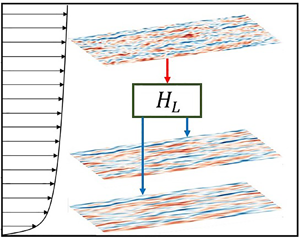
Transfer function-based methods have more recently been used for the estimation of large-scale fluctuations in wall-bounded turbulent flows (Marusic, Mathis & Hutchins Reference Marusic, Mathis and Hutchins2010; Mathis, Hutchins & Marusic Reference Mathis, Hutchins and Marusic2011; Baars, Hutchins & Marusic Reference Baars, Hutchins and Marusic2016; Suzuki & Hasegawa Reference Suzuki and Hasegawa2017; Illingworth, Monty & Marusic Reference Illingworth, Monty and Marusic2018; Madhusudanan, Illingworth & Marusic Reference Madhusudanan, Illingworth and Marusic2019; Encinar & Jiménez Reference Encinar and Jiménez2019; Sasaki et al. Reference Sasaki, Vinuesa, Cavalieri, Schlatter and Henningson2019; Amaral et al. Reference Amaral, Cavalieri, Martini, Jordan and Towne2020; Martini et al. Reference Martini, Cavalieri, Jordan, Towne and Lesshafft2020; Towne, Lozano-Durán & Yang Reference Towne, Lozano-Durán and Yang2020). These methods are loosely based on the concept that large energy-containing eddies are ‘attached’ to the wall (Townsend Reference Townsend1976) and therefore that their measurements at one wall-normal location can be used to estimate these ‘attached’ eddies at other wall-normal locations. (The term ‘attached’ means that these eddies extend to the wall such that they can feel the presence of the wall but are not necessarily physically connected to the wall Marusic & Monty (Reference Marusic and Monty2019).) The underlying transfer functions are usually generated (i) either from two-point correlations of previously collected data at the measurement and estimation locations (e.g. Mathis et al. Reference Mathis, Hutchins and Marusic2011), or (ii) from resovent-based method where time-resolved data at only the measurement location is used in combination with a Navier–Stokes (NS)-based linear model (e.g. Towne et al. Reference Towne, Lozano-Durán and Yang2020). In the present study, we follow the work of Madhusudanan et al. (Reference Madhusudanan, Illingworth and Marusic2019), where NS-based linear models are used to obtain the transfer functions such that no previously collected data, other than the mean velocity profile, is required. This method provides instantaneous estimates at multiple locations from instantaneous measurements (i.e. a single snapshot) at one wall-normal location. Our focus is on improving the performance of such NS-based linear models.
1.1. Structure of wall turbulence and inner–outer interactions
In wall-bounded turbulent flows, the wall segregates the flow into different regions: (i) an inner region close to the wall where viscous effects are important and the relevant length scale is  $\nu /u_{\tau }$ ( $\nu$ is the kinematic viscosity, $u_{\tau }= \sqrt {\tau /\rho }$ is the friction velocity, $\tau$ is the mean shear stress at the wall and $\rho$ is the flow density); (ii) an outer region away from the wall where inertial effects are important and the relevant length scale is $h$, which can be the channel half-width or boundary-layer thickness; and (iii) the overlap region (logarithmic region) where the inner to outer region transition occurs and the relevant length scale is the distance from the wall (von Kármán Reference von Kármán1931; Jiménez Reference Jiménez2013). The ratio of the outer to inner length scales is the friction Reynolds number ( $Re_{\tau } = u_{\tau }h/\nu$), which quantifies the range of length scales involved and hence the complexity of the flow.
Turbulent energy in wall-bounded flows is generated by shear above the wall and is therefore maximum close to the wall, just above the viscous sublayer (Townsend Reference Townsend1976). This region is referred to as the near-wall region and it lies between the wall and the logarithmic region (see figure 1). This near-wall region is very thin in engineering and environmental flows for which  $Re_{\tau } = 10^{3} - 10^{7}$. It makes numerical calculations (Jiménez Reference Jiménez2003; Smits & Marusic Reference Smits and Marusic2013) or experimental measurements (McKeon et al. Reference McKeon, Li, Jiang, Morrison and Smits2004; Hutchins et al. Reference Hutchins, Nickels, Marusic and Chong2009; Hultmark et al. Reference Hultmark, Vallikivi, Bailey and Smits2012) of fluctuations in this region prohibitively expensive in most situations. Instead, there is an interest in exploiting the coupling between the inner- and outer-region events to estimate fluctuations in the near-wall region from measurements in the logarithmic region.
(a) Cess (Reference Cess1958) approximation of the eddy viscosity and (b) the corresponding mean velocity profile (the  $z$-axes are square root scaled). (c) Instantaneous streamwise velocity fields in the horizontal planes at $z^{+} = 300$, $100$ and $10$.
$10$.

Marusic et al. (Reference Marusic, Mathis and Hutchins2010) and Mathis et al. (Reference Mathis, Hutchins and Marusic2011) developed such a predictive model which exploits two kinds of inner–outer interactions. First, large-scale fluctuations in the outer region are observed to impose their ‘footprint’ in the near-wall region (Abe, Kawamura & Choi Reference Abe, Kawamura and Choi2004; Hutchins & Marusic Reference Hutchins and Marusic2007a; Baars, Hutchins & Marusic Reference Baars, Hutchins and Marusic2017). (The term ‘footprint’ means that large-scale fluctuations that are generated in the outer region extend their influence to the near-wall region Mathis et al. (Reference Mathis, Hutchins and Marusic2011).) This ‘footprint’ component therefore describes large-scale fluctuations close to the wall. Second, in addition to imposing their ‘footprint’, the large-scale fluctuations in the outer region are also observed to modulate the near-wall cycle, which generates near-wall streaks and vortices (Rao, Narasimha & Narayanan Reference Rao, Narasimha and Narayanan1971; Brown & Thomas Reference Brown and Thomas1977; Bandyopadhyay & Hussain Reference Bandyopadhyay and Hussain1984; Hutchins & Marusic Reference Hutchins and Marusic2007b; Mathis, Hutchins & Marusic Reference Mathis, Hutchins and Marusic2009). This modulation component, therefore, describes small-scale fluctuations, i.e. the near-wall streaks and vortices, close to the wall.
At high Reynolds numbers, large-scale fluctuations (i) account for most of the turbulence production (Hultmark et al. Reference Hultmark, Vallikivi, Bailey and Smits2012) and (ii) increasingly modulate the near-wall cycle (Mathis et al. Reference Mathis, Hutchins and Marusic2009). (The near-wall cycle still remains self-sustained (Jiménez & Pinelli Reference Jiménez and Pinelli1999; Schoppa & Hussain Reference Schoppa and Hussain2002). However, in high- $Re_{\tau }$ flows, the amplitude of the resulting near-wall streaks and vortices is strongly correlated to the amplitude of large-scale fluctuations in the logarithmic region.) For these two reasons, it is expected that the importance of large-scale fluctuations increases with $Re_{\tau }$ and these fluctuations therefore form the primary focus of this study.
1.2. Spectral linear stochastic estimation of large-scale fluctuations
Baars et al. (Reference Baars, Hutchins and Marusic2016) noted that the predictive model of Marusic et al. (Reference Marusic, Mathis and Hutchins2010) and Mathis et al. (Reference Mathis, Hutchins and Marusic2011) could be improved by applying spectral linear stochastic estimation (SLSE) for the estimation of large-scale fluctuations. Mathis et al. (Reference Mathis, Hutchins and Marusic2011) designed their model from the cross-correlation of large-scale streamwise velocity fluctuations at the measurement location ( $z_m$) and estimation location ( $z_p$); $z_m$ and $z_p$ are separated in the wall-normal direction only. This is essentially stochastic estimation in which conditional averages between two variables are obtained from unconditional statistics. Adrian (Reference Adrian1979) proposed that the estimation of a fluctuating velocity component $u_{i}(z_p)$ from measurements of the state-vector $\boldsymbol {u}(z_m)$ can be approximated using a Taylor-series expansion as
 \begin{equation} u_{ip}(z_p,t) = A_{ij}(z_m,z_p)u_{jm}(z_m,t) + B_{ijk}(z_m,z_p)u_{jm}(z_m,t)u_{km}(z_m,t) + \ldots, \end{equation}
where  $A_{ij}$, $B_{ijk}$ are second- and third-order two-point correlation tensors, respectively, subscripts $i,j,k$ indicate components of the state-vector $\boldsymbol {u}$ and subscripts $m$ and $p$ indicate the measured and estimated quantities, respectively. We now limit ourselves to the first term only, i.e. to linear stochastic estimation (LSE), which has been shown to be a good approximation in wall-bounded turbulent flows (Guezennec Reference Guezennec1989; Baars et al. Reference Baars, Hutchins and Marusic2016; Encinar & Jiménez Reference Encinar and Jiménez2019; Sasaki et al. Reference Sasaki, Vinuesa, Cavalieri, Schlatter and Henningson2019). In LSE, the coefficient $A_{ij}(z_m,z_p)$, obtained by minimizing the mean square error, is given by the two-point correlation tensor $\langle u_j(z_m,t) u_i(z_p,t) \rangle / \langle |u_j(z_m,t)|^{2} \rangle$, where $\langle \rangle$ denotes ensemble averaging.
The LSE can be improved when performed in the spectral domain (Tinney et al. Reference Tinney, Coiffet, Delville, Hall, Jordan and Glauser2006), because SLSE preserves spectral structure and eliminates any contamination caused by correlations between orthogonal spectral modes. Following Mathis et al. (Reference Mathis, Hutchins and Marusic2011), we assume that both measurements and estimation are performed for the streamwise velocity fluctuations, and drop the subscripts  $(i,j,k)$. The flow is homogeneous in the streamwise and spanwise directions so we decompose the velocity fluctuations into their Fourier coefficients characterized by the streamwise and spanwise wavenumbers $(k_x,k_y)$. This transforms the linear contribution of (1.1) into
 \begin{gather} \hat{u}_p(z_p,t;k_x,k_y) = H_L(z_p,z_m;k_x,k_y)\hat{u}_m(z_m,t;k_x,k_y), \end{gather}
 \begin{gather}H_L(z_p,z_m;k_x,k_y) = \frac{\langle \hat{u}(z_p,t;k_x,k_y) \hat{u}^{{{\dagger}}}(z_m,t;k_x,k_y) \rangle}{\langle \hat{u}(z_m,t;k_x,k_y) \hat{u}^{{{\dagger}}}(z_m,t;k_x,k_y) \rangle}, \end{gather}
where  $\;\hat {}\;$ denotes the Fourier coefficient and superscript $^{{\dagger} }$ denotes the complex conjugate. We do not perform a Fourier transform in time because we aim to obtain instantaneous estimations from instantaneous measurements as discussed in § 3. In order to gain better insight, following Baars et al. (Reference Baars, Hutchins and Marusic2016), we further break the transfer function $H_L$ into
 \begin{gather} |H_L(z_p,z_m;k_x,k_y)| = \sqrt{\gamma^{2}(z_p,z_m;k_x,k_y)\frac{\langle |\hat{u}(z_p,t;k_x,k_y)|^{2} \rangle}{\langle |\hat{u}(z_m,t;k_x,k_y)|^{2} \rangle} }, \end{gather}
 \begin{gather}\gamma^{2}(z_p,z_m;k_x,k_y) = \frac{|\langle \hat{u}(z_p,t;k_x,k_y) \hat{u}^{{{\dagger}}}(z_m,t;k_x,k_y) \rangle|^{2}}{\langle |\hat{u}(z_p,t;k_x,k_y)|^{2} \rangle \langle |\hat{u}(z_m,t;k_x,k_y)|^{2} \rangle}, \end{gather}
where  $\gamma ^{2}$ is the two-dimensional linear coherence spectrum (2-D LCS) between the measurement and estimation locations. For fluctuations of the wavenumber pair $(k_x,k_y)$, $\gamma ^{2} = 1$ implies that all fluctuations of that wavenumber pair at $z_m$ are linearly correlated with those at $z_p$ (i.e. perfect coherence). In contrast, $\gamma ^{2} = 0$ implies that all fluctuations of that wavenumber pair at $z_m$ are linearly uncorrelated with those at $z_p$ (i.e. no coherence).
1.3. NS-based linear models for SLSE
Linear stochastic estimation, in general, requires simultaneous measurements (or numerical data) at two wall-normal locations ( $z_m$ and $z_p$) to obtain the transfer function $H_L$. In an alternative approach, Madhusudanan et al. (Reference Madhusudanan, Illingworth and Marusic2019) obtain $H_L$ using NS-based linear models. This removes the need for measurements at the estimation location $z_p$ entirely. As a consequence, fluctuations at several wall-normal locations, including very close to the wall, can be predicted from measurements at just one wall-normal location. These linearized models are created by first forming the nonlinear equations governing the evolution of velocity fluctuations by applying the Reynolds decomposition to the NS equations,
 \begin{equation} \frac{\partial u_i}{\partial t} ={-}U_k \frac{\partial u_i}{\partial x_k} - u_k\frac{\partial U_i}{\partial x_k} - \frac{\partial }{\partial x_k}\left(u_k u_i - \langle u_k u_i\rangle\right) - \frac{1}{\rho}\frac{\partial p}{\partial x_i} + \nu\frac{\partial^{2}u_i}{\partial x_k \partial x_k}, \end{equation}
where  $U_i$ is the mean velocity and $u_i$ and $p$ are the velocity and pressure fluctuations, respectively. We could directly obtain the evolution equations for the covariance matrices required for LSE in (1.1) and SLSE in (1.2b) from this equation. This is difficult because the third term on the right-hand side of (1.4) is nonlinear and can only be solved with computationally expensive simulations, which we aim to avoid. An estimation method for wall turbulence based on the full NS equations has been recently implemented by Wang & Zaki (Reference Wang and Zaki2020) for a channel flow at $Re_{\tau } = 180$.
The easiest approximation would be to ignore the nonlinear term altogether. This may be justified because the nonlinear term in the NS equations is energy conserving. The energy extracted from the mean flow, which leads to energetic large-scale fluctuations, is therefore attributable to the linear terms alone (Joseph Reference Joseph1976). The linear terms alone, however, cannot sustain wall turbulence (Mckeon Reference Mckeon2017). The nonlinear term plays an essential role in energy extraction (Jiménez Reference Jiménez2018) and thus cannot be ignored entirely. McKeon & Sharma (Reference McKeon and Sharma2010) treat the nonlinear term as an unknown forcing, thus avoiding the need to either ignore or model it. Resolvent analyses, which are linear, based on this approach reproduce many qualitative features of wall turbulence (McKeon & Sharma Reference McKeon and Sharma2010; Moarref et al. Reference Moarref, Sharma, Tropp and McKeon2013; Sharma & Mckeon Reference Sharma and Mckeon2013), thus showing the importance of the linear terms in nonlinear turbulent flows. Another alternative is to model the nonlinear term as stochastic excitation, thus transforming the system into a linear stochastic model. Farrell & Ioannou (Reference Farrell and Ioannou1998) showed that stochastically excited turbulent boundary layers exhibit energy spectra distinctly similar to those in boundary-layer turbulence. Later, Hwang & Cossu (Reference Hwang and Cossu2010) included an eddy dissipation term along with the stochastic excitation term to obtain an alternative NS-based linear model,
 \begin{equation} \frac{\partial u_i}{\partial t} ={-}U_k \frac{\partial u_i}{\partial x_k} - u_k\frac{\partial U_i}{\partial x_k} + \frac{\partial}{\partial x_k}\left(\nu_t\left(\frac{\partial u_i}{\partial x_k}+\frac{\partial u_k}{\partial x_i}\right)\right) + \sigma d(\boldsymbol{x},t) - \frac{1}{\rho}\frac{\partial p}{\partial x_i} + \nu\frac{\partial^{2}u_i}{\partial x_k \partial x_k}, \end{equation}
where  $\nu _t$ is the eddy viscosity and $d(x,t)$ is a spatially uniform white-in-time body forcing of intensity $\sigma$. The inclusion of the eddy dissipation term is mainly motivated by the studies of Reynolds & Hussain (Reference Reynolds and Hussain1972) and del Álamo & Jiménez (Reference del Álamo and Jiménez2006), who showed it to be useful in modelling the dissipative effect of background turbulence. Illingworth et al. (Reference Illingworth, Monty and Marusic2018) also found that the inclusion of the eddy dissipation term is important for the evolution and hence the estimation of large-scale fluctuations in wall turbulence. Madhusudanan et al. (Reference Madhusudanan, Illingworth and Marusic2019) showed that (1.5) can be effectively used to obtain the transfer function $H_L$ in (1.2b) without requiring any previously collected data other than the mean velocity profile (see § 4). They thus obtained estimations of the large-scale velocity fluctuations at several wall-normal locations from instantaneous measurements at one wall-normal location.
We note that, as well as LSE/SLSE, there are other methods where NS-based linear models, such as (1.5), have been used for estimating the large-scale velocity fluctuations in wall turbulence. These include Kalman filter-based optimal estimators (Hœpffner et al. Reference Hœpffner, Chevalier, Bewley and Henningson2005; Chevalier et al. Reference Chevalier, Hæpffner, Bewley and Henningson2006; Colburn, Cessna & Bewley Reference Colburn, Cessna and Bewley2011; Illingworth et al. Reference Illingworth, Monty and Marusic2018) and resolvent-based estimators (Amaral et al. Reference Amaral, Cavalieri, Martini, Jordan and Towne2020; Martini et al. Reference Martini, Cavalieri, Jordan, Towne and Lesshafft2020; Towne et al. Reference Towne, Lozano-Durán and Yang2020). On the one hand, as opposed to the method of Madhusudanan et al. (Reference Madhusudanan, Illingworth and Marusic2019), these methods need time-resolved measurement data. On the other hand, these methods can consider coloured-in-time forcing. Although the colour of the forcing statistics is important (Nogueira et al. Reference Nogueira, Morra, Martini, Cavalieri and Henningson2021; Zare, Jovanović & Georgiou Reference Zare, Jovanović and Georgiou2017), the inclusion of the eddy viscosity term in (1.5) partly compensates for the lack of colour in the white-in-time forcing as noted by Zare et al. (Reference Zare, Jovanović and Georgiou2017) and Morra et al. (Reference Morra, Semeraro, Henningson and Cossu2019, Reference Morra, Nogueira, Cavalieri and Henningson2021).
1.4. Contributions of the present study
Madhusudanan et al. (Reference Madhusudanan, Illingworth and Marusic2019) showed that when the NS-based linear model (1.5) is used for stochastic estimation, the results are significantly improved when compared with those from a model without the eddy dissipation term. There are, however, still serious limitations associated with the eddy dissipation and forcing terms used in (1.5). This limits the applications of (1.5) to cases where both the measurement and estimation locations are in the logarithmic region. It is not suitable when one of these two locations is close to the wall, such as in the near-wall region, which is a requirement in many practical situations (Encinar & Jiménez Reference Encinar and Jiménez2019; Marusic et al. Reference Marusic, Mathis and Hutchins2010). This limitation is explained by the fact that (1.5) captures the coherence of large-scale fluctuations only within the logarithmic region but not across the logarithmic and near-wall regions. Qualitatively similar results are also reported by Illingworth et al. (Reference Illingworth, Monty and Marusic2018) who use the same model but with a Kalman filter-based optimal estimator. In this paper, we therefore aim to improve the design of NS-based linear models to obtain better estimation within the logarithmic region as well as across the logarithmic and near-wall regions.
In this paper, we choose a turbulent channel flow at  $Re_{\tau } = 2000$ as a representative wall-bounded turbulent flow (§ 2). Based on a physics-based approach, we modify the eddy dissipation and stochastic forcing terms in (1.5) such that they better represent the nonlinear interactions (§ 3) and formulate the models using an input–output framework (§ 4). We then use these linear models for estimation of large-scale fluctuations (§ 5) and gain new insights based on their ability to capture the linear production term (§ 6). Finally, we discuss the scope and limitations of the present study (§ 7).
2. Incompressible fully developed turbulent channel flow
We consider a fully developed incompressible turbulent flow in a channel of half-width  $h$ at $Re_{\tau } = 2000$ (the same as that studied by Madhusudanan et al. (Reference Madhusudanan, Illingworth and Marusic2019)). The evolution of velocity fluctuations in this flow is governed by (1.4), where subscripts take values $(1,2,3)$ and refer to coordinates $(x,y,z)$ denoting the streamwise, spanwise and wall-normal directions, respectively. The mean and fluctuating velocity fields are represented as $(U,0,0)$ and $(u,v,w)$, respectively. To complete the model described by (1.5), we require the mean velocity profile, which is fixed for a given flow, and the eddy viscosity profile, which depends on our definition. Following Reynolds & Hussain (Reference Reynolds and Hussain1972) and many others, we use the Cess (Reference Cess1958) approximation of $\nu _t$ given as
 \begin{equation} \nu_t = \frac{\nu}{2}\left(1 + \frac{\kappa^{2} Re_{\tau}^{2}}{9}(2z-z^{2})^{2}(3- 4z+2z^{2})^{2}\left[1 - \exp\left({-}z \frac{Re_{\tau}}{A}\right)\right]^{2} \right)^{1/2} - \frac{\nu}{2}, \end{equation}
where  $z$ is the wall distance non-dimensionalized by $h$ and $(\kappa ,A) = (0.426, 25.4)$ have been calibrated at $Re_{\tau } = 2000$ by del Álamo & Jiménez (Reference del Álamo and Jiménez2006). This eddy viscosity is defined such that the mean velocity $U$ can be obtained by integrating $Re_{\tau }(1-z)/(\nu _t+\nu )$ in the wall-normal direction. Figure 1 shows $\nu _t^{+}$ and $U^{+}$ profiles (superscript $^{+}$ denotes non-dimensionalization in inner units). This figure also shows the outer (from $z^{+} = 30$ to $z = 1$), inner (from the wall to $z = 0.15$), logarithmic (overlap region) and near-wall (between the wall and logarithmic region) regions. (Note that the viscous sublayer ( ${z^{+} < 5}$) is the lower part of the near-wall region where the flow remains mostly laminar.) This division is only nominal (Marusic et al. Reference Marusic, Mathis and Hutchins2010). The logarithmic region is otherwise clearly observed only at much higher $Re_{\tau }$ (Hultmark et al. Reference Hultmark, Vallikivi, Bailey and Smits2012).
We fix the measurement plane at  $z_m^{+} \approx 300$ throughout this study and vary the estimation planes from $z_p^{+} \approx 200$ to 10. We choose the measurement plane to be as far away from the wall as possible while still being within the nominal logarithmic region. The wall-normal location $z_m = 0.15$ (i.e. $z_m^{+} = 300$) is close to the upper limit of the nominal logarithmic region, which is also observed to be the case for channel flow at $Re_{\tau } \approx 5200$ by Lee & Moser (Reference Lee and Moser2015). However, we note that this is still a relatively low $Re_{\tau }$ flow in which the true logarithmic region, characterized by constant $z \,\textrm {d}U/\textrm {d}z$, does not exist (Lee & Moser Reference Lee and Moser2015). Therefore, the results presented in this study cannot be extended to higher $Re_{\tau }$ flows with complete certainty, as discussed in § 7.3. We also note that the wall-normal location $z_p^{+} = 10$ is certainly in the viscous-dominated near-wall region where $\nu _t < \nu$ and the mean shear is high.
The direct numerical simulation (DNS) data for streamwise velocity fluctuations is provided by the Polytechnic University of Madrid. The simulation was carried out in a computational domain of size  $8{\rm \pi} h \times 3{\rm \pi} h \times 2h$ in the streamwise, spanwise and wall-normal directions. The domain was periodic in the horizontal directions and discretized using 2048 Fourier components in each direction, the wall-normal direction was discretized using a seven-point compact finite difference scheme with 512 points. Temporal integration was performed using a semi-implicit third-order low-storage Runge–Kutta scheme (see Vela-Martín et al. (Reference Vela-Martín, Encinar, García-Gutiérrez and Jiménez2019) for further details). We use only a subset of the simulated wavenumbers, which satisfy $0.25\leqslant |k_x|\leqslant 8.0$ and $0.66\leqslant |k_y|\leqslant 21.0$ (non-dimensionalized by $h$). The corresponding non-dimensional wavelengths are $0.8\lesssim |\lambda _x|\lesssim 25.0$ and $0.3\lesssim |\lambda _y| \lesssim 9.5$, where $\lambda _x = 2{\rm \pi} /k_x$ and ${\lambda _y = 2{\rm \pi} /k_y}$. Instantaneous streamwise velocity fields in three horizontal planes at $z^{+} = 300$, 100 and 10 are shown in figure 1(c). They share many common features, thus indicating important correlations between the different wall-normal locations.
3. Design of NS-based linear models
We write (1.4) in the spectral domain by applying the Fourier transformation in the horizontal directions as
 \begin{equation} \frac{\partial \hat{u}_i}{\partial t} ={-}U_k \frac{\partial \hat{u}_i}{\partial x_k} - \hat{u}_k\frac{\partial U_i}{\partial x_k} - \frac{\partial }{\partial x_k}\left(\widehat{u_k u_i}\right) - \frac{1}{\rho}\frac{\partial \hat{p}}{\partial x_i} + \nu\frac{\partial^{2}\hat{u}_i}{\partial x_k \partial x_k}, \end{equation}
where, as in § 1.2,  $\;\hat {}\;$ denotes a Fourier coefficient and the operators $\partial /\partial x_1$, $\partial /\partial x_2$, $\partial ^{2}/\partial x_1^{2}$ and $\partial ^{2}/\partial x_2^{2}$ are equivalent to multiplication by $\textrm {i}k_x$, $\textrm {i}k_y$, $-k_x^{2}$ and $-k_y^{2}$, respectively. All the models in the present study are designed by replacing the nonlinear term (third term on the right-hand side) by a combination of an eddy dissipation term and a white-in-time spatially distributed body-forcing term. The resulting NS-based linear models are then represented as
 \begin{equation} \frac{\partial \hat{u}_i}{\partial t} ={-}U_k \frac{\partial \hat{u}_i}{\partial x_k} - \hat{u}_k\frac{\partial U_i}{\partial x_k} + \frac{\partial}{\partial x_k}\left(f_{\nu}\left(\frac{\partial \hat{u}_i}{\partial x_k}+\frac{\partial \hat{u}_k}{\partial x_i}\right)\right) + f_{\sigma} \hat{d} - \frac{1}{\rho}\frac{\partial \hat{p}}{\partial x_i} + \nu\frac{\partial^{2}\hat{u}_i}{\partial x_k \partial x_k}, \end{equation}
where  $f_{\nu }$ and $f_{\sigma }$ are, in general, functions of the wall-normal distance $z$ and the wavenumbers $k_x$ and $k_y$ (see table 1).
Summary of the NS-based linear models used in the present study.

In the derivation of the linear models in the present study, we do not perform a Fourier transform in time. This is because the Fourier transform is inherently non-local (Farge Reference Farge1992), which means that if we perform a Fourier transform in time then local time information will be lost. The estimation at one time instant will then need time-resolved data from  $t = -\infty$ to $\infty$. In cases where the relationship between the estimated and measured quantities is mostly causal, the estimation could be approximated using the past measurements alone (i.e. $t = -\infty$ to $0$) as shown by Sasaki et al. (Reference Sasaki, Vinuesa, Cavalieri, Schlatter and Henningson2019). It is also worth noting that because we do not perform a Fourier transform in time, the calculation of the transfer function ( $H_L$ in (1.2b)) also only requires snapshots of velocity fluctuations at $z_m$ and $z_p$ and not time-resolved data. This simplification has a direct parallel with the calculation of proper orthogonal decomposition (known as POD) modes rather than spectral proper orthogonal decomposition modes (Towne, Schmidt & Colonius Reference Towne, Schmidt and Colonius2018). One could imagine that, by not using time-resolved data, we are losing possibly important temporal correlation information. This can be understood from the fact that the stochastic forcing term in (3.2) is restricted to be white-in-time. Although the colour of the forcing statistics is shown to be crucial in many recent studies (Zare et al. Reference Zare, Jovanović and Georgiou2017; Nogueira et al. Reference Nogueira, Morra, Martini, Cavalieri and Henningson2021), we still keep the simplification of white-in-time forcing in the present study. This is because the inclusion of the eddy viscosity term in the linear models approximately plays the same role as the colour in the forcing statistics (Zare et al. Reference Zare, Jovanović and Georgiou2017; Morra et al. Reference Morra, Semeraro, Henningson and Cossu2019, Reference Morra, Nogueira, Cavalieri and Henningson2021).
3.1. Baseline model (the B-model)
Turbulent fluctuations interact across wavenumbers via the nonlinear term in (3.1), which is modelled as a combination of an eddy dissipation term and a stochastic body-forcing term in (3.2). This approach is phenomenological, i.e. (3.2) is not derived from first principles. The eddy dissipation term is supposed to model the dissipative effect of the background turbulence, i.e. small-scale fluctuations, and is often modelled by setting  $f_{\nu } = \nu _t$ in the literature. This follows the work of Reynolds & Hussain (Reference Reynolds and Hussain1972), who used this eddy dissipation term to heuristically model the dissipation of turbulent fluctuations in the presence of externally imposed harmonic fluctuations. In contrast, the stochastic body forcing term is supposed to model the excitation by turbulent fluctuations and is often modelled by setting $f_{\sigma } = \sigma$ (a constant). This follows the work of Jovanović & Bamieh (Reference Jovanović and Bamieh2005), who used this term to heuristically model turbulence excitation in laminar channel flows. As noted by Jimenez (Reference Jimenez2009), such NS-based linear models are crude, and therefore any results generated with them need to be relatively insensitive to the details of $f_{\nu }$ and $f_{\sigma }$.
We refer to the model from the literature in which  $f_{\nu } = \nu _t$ and $f_{\sigma } = \sigma$ as the baseline model or the B-model (table 1). This model is used by Madhusudanan et al. (Reference Madhusudanan, Illingworth and Marusic2019) and others; it has a wall-distance-dependent eddy dissipation term and a spatially uniform stochastic forcing term. We need not fix the value of $\sigma$, which quantifies the magnitude of stochastic forcing, because the transfer function $H_L$ (see (1.2b)) is calculated from the ratio of turbulent fluctuations at $z_m$ and $z_p$. Therefore, $H_L$ depends only on the spatial structure of $f_{\sigma }$ and not on its magnitude. Information concerning the magnitude of fluctuations is estimated at $z_p$ from the magnitude of fluctuations measured at $z_m$ (see (1.2a)).
3.2. Wall-distance-dependent nonlinear interactions (the W-model)
The eddy dissipation and stochastic forcing terms model the nonlinear interactions of turbulent fluctuations. Since turbulent fluctuations are wall-distance-dependent, these two terms are also expected to be wall-distance-dependent. As the simplest possible modification of the B-model, we set  $f_{\sigma } = \sigma \nu _t$ and keep $f_{\nu } = \nu _t$. We call this model the W-model (table 1); it has eddy dissipation and stochastic-forcing terms that are each wall-distance-dependent. To justify our approximation intuitively we first assume that the eddy dissipation term predominantly models the energy transfer to other scales while the stochastic-forcing term predominantly models the energy transfer from other scales. It is known that these two energy-transfer mechanisms balance each other at most wall-normal locations (Mizuno Reference Mizuno2016; Lee & Moser Reference Lee and Moser2019; Hwang & Lee Reference Hwang and Lee2020), so we expect the two terms ( $f_{\nu }$ and $f_{\sigma }$) to vary in proportion to each other. We will see from the results concerning turbulence statistics in § 6 that this approximation indeed works well.
3.3. Scale-dependent nonlinear interactions (the  $\lambda$-model)

The nonlinear interactions through which turbulent fluctuations interact are scale dependent (Cho, Hwang & Choi Reference Cho, Hwang and Choi2018). We therefore expect  $f_{\nu }$ and $f_{\sigma }$ also to be scale dependent. This has also been previously suggested for the $f_{\nu }$ term by Jimenez (Reference Jimenez2009) and Illingworth et al. (Reference Illingworth, Monty and Marusic2018), who noted that the eddy viscosity $\nu _t$ could over-damp fluctuations and that $f_{\nu }$ should be smaller at smaller scales. The challenge is to incorporate this scale dependence without restricting the model's applicability to a specific case. We therefore base the design of our scale-dependent model, which we call the ${\lambda }$-model (table 1), on two observations that are common to all wall-bounded turbulent flows.
The first observation we use is that energy transfer occurs mainly from the large, energy-containing eddies to smaller eddies (a notable exception is small but significant energy transfer from the near-wall streaks to larger scales in the near-wall region). This means that  $f_{\nu }$ should be approximately zero for fluctuations of length scales much smaller than those of the energy-containing eddies and should approach its maximum value (which we assume to be $\nu _t$) for fluctuations of length scales of the order of the length scale of the energy-containing eddies. In order to incorporate such scale dependence, we define the length scale of a Fourier component as $\lambda \equiv 2{\rm \pi} /(k_x^{2}+k_y^{2})^{0.5}$, the same as those used by Lee & Moser (Reference Lee and Moser2019). We then set $f_{\nu } = s\nu _t$ where $s(\lambda ;z) = \lambda /(\lambda + \lambda _m)$ is a multiplicative factor that is zero at $\lambda = 0$, increases rapidly at $\lambda \approx \lambda _m$, and approaches one as $\lambda \to \infty$ (see figure 2a). The parameter $\lambda _m$ (whose value is given below) roughly quantifies a lower bound for the length scale of the energy-containing eddies.
(a) The multiplicative factor  $s = \lambda /(\lambda +\lambda _m)$ (thick black line) is approximately zero at small scales and approaches one for $\lambda > \lambda _m$. The thin blue lines show variants of $s$:
$s$:  $(\lambda /(\lambda +\lambda _m))^{0.5}$ (above) and $(\lambda /(\lambda +\lambda _m))^{1.5}$ (below). The thin red line shows $\lambda _m/(\lambda + \lambda _m)$, which has the opposite trend to that of $s$. (b) Here $\lambda _m = a + b\tanh (cz)$ (thick black line) approximates a lower bound for the length scale of energy-containing eddies as a function of the wall distance. The thin blue lines show $0.5 \lambda _m$ (above) and $2.0 \lambda _m$ (below). The thin red line shows $(a+b)- b\tanh (cz)$, which has the opposite trend to that of $\lambda _m$.

The second observation we use is that, in wall turbulence, the length scale of the energy-containing eddies depends on their distance from the wall (Jiménez Reference Jiménez2012). We therefore set  $\lambda _m$ to be a hyperbolic function $\lambda _m(z) = a + b\tanh (cz)$, where $a = 50/Re_{\tau }$ is of the order of the energy-containing eddies in the near-wall region, $a+b = 2$ is of the order of the energy-containing eddies at the channel centre and $c = 6$ is such that the length scale of the energy-containing eddies plateaus at the end of the logarithmic region. Figure 2(b) shows that $\lambda _m$ scales linearly with $z$ in the logarithmic region and then plateaus in the outer region, similar to the scaling of the energy-containing eddies in wall turbulence (Jiménez Reference Jiménez2012). Finally, following our arguments in § 3.2 on the energy-transfer balance, we set the stochastic forcing intensity to be proportional to the eddy dissipation term, i.e. $f_{\sigma } = \sigma s \nu _t$.
It should be noted that we do not optimize either the parameters  $a$,
$a$,  $b$ and $c$ or the forms of the functions $s$ and $\lambda _m$ to match the model with observations. In fact, the model results should remain qualitatively unchanged provided that $s$ and $\lambda _m$ follow the trends described above. This is demonstrated in the Appendix where the influence of variations in $s$ and $\lambda _m$ (thin lines in figure 2) is analysed.
4. Input–output formulation
We now write the NS-based linear models (3.2) in the Orr–Sommerfeld–Squire form (see Jovanović & Bamieh Reference Jovanović and Bamieh2005), which is more convenient for input–output analysis, as
 \begin{gather} \frac{\partial \hat{\boldsymbol{q}}}{dt} = \boldsymbol{A}\hat{\boldsymbol{q}} + \boldsymbol{B}\hat{\boldsymbol{d}}, \end{gather}
 \begin{gather}\hat{\boldsymbol{u}} = \boldsymbol{C}\hat{\boldsymbol{q}}, \end{gather}
where  $\hat {\boldsymbol {q}} = (\hat {w},\hat {\eta })$ comprises the wall-normal velocity and vorticity fluctuations. The linear operators $\boldsymbol {A}$ and $\boldsymbol {C}$ are similar to those in Hwang & Cossu (Reference Hwang and Cossu2010) and the operator $\boldsymbol {B}$ is similar to that in Ran et al. (Reference Ran, Zare, Hack and Jovanović2019). They are given by
 \begin{gather} \boldsymbol{A} = \begin{bmatrix} \varDelta^{{-}1}\mathcal{L}_{OS} & 0\\ -\textrm{i}k_y\partial_z U & \mathcal{L}_{SQ}\end{bmatrix}, \end{gather}
 \begin{gather}\boldsymbol{B} = \begin{bmatrix} -\textrm{i}k_x\varDelta^{{-}1}\left(f_{\sigma}\mathcal{D} + \partial_zf_{\sigma}\right) & -\textrm{i}k_y\varDelta^{{-}1}\left(f_{\sigma}\mathcal{D} + \partial_zf_{\sigma}\right) & -k^{2}\varDelta^{{-}1}\\ -\textrm{i}k_yf_{\sigma} & -\textrm{i}k_xf_{\sigma} & 0\end{bmatrix}, \end{gather}
 \begin{gather}\boldsymbol{C} = \frac{1}{k^{2}} \begin{bmatrix} \textrm{i}k_x\mathcal{D} & -\textrm{i}k_y\\ \textrm{i}k_y\mathcal{D} & \textrm{i}k_x\\ k^{2} & 0 \end{bmatrix}, \end{gather}
where  $\varDelta = \mathcal {D}^{2} - k^{2}$, $k^{2} = k_x^{2} + k_y^{2}$ and $\mathcal {D}$ and $\partial _z$ represent differentiation in the wall-normal direction. The operators $\mathcal {L}_{OS}$ and $\mathcal {L}_{SQ}$ are
 \begin{gather} \mathcal{L}_{OS} ={-}\textrm{i}k_xU\varDelta + \textrm{i}k_x\partial^{2}_zU + \left(f_{\nu}+\nu\right)\varDelta^{2} + 2\partial_z f_{\nu}\mathcal{D}\varDelta + \partial^{2}_zf_{\nu}\left(\mathcal{D}^{2}+k^{2}\right), \end{gather}
 \begin{gather}\mathcal{L}_{SQ} = \textrm{i}k_xU + \left(f_{\nu} + \nu\right)\varDelta + \partial_z f_{\nu}\varDelta. \end{gather}
Because the system is linearly stable, i.e. all the eigenvalues of  $\boldsymbol {A}$ are stable, and the stochastic forcing is white-in-time, the system's response can be calculated in terms of the covariance tensor $\boldsymbol {X} = \langle \hat {\boldsymbol {q}} \hat {\boldsymbol {q}}^{{\dagger} }\rangle$ by solving the algebraic Lyapunov equation (Hwang & Cossu Reference Hwang and Cossu2010),
 \begin{equation} \boldsymbol{A}\boldsymbol{X} + \boldsymbol{X}\boldsymbol{A}^{{{\dagger}}} + \boldsymbol{B}\boldsymbol{B}^{{{\dagger}}} = 0. \end{equation}
We calculate the covariance tensor  $\langle \hat {\boldsymbol {u}} \hat {\boldsymbol {u}}^{{\dagger} }\rangle$ required for calculation of $H_L$ in (1.2b) as $\boldsymbol {C}\boldsymbol {X} \boldsymbol {C}^{{\dagger} }$. To discretize the operators $\boldsymbol {A}$, $\boldsymbol {B}$ and $\boldsymbol {C}$ in the wall-normal direction (from $z = 0$ to $1$), we use a Chebyshev-collocation method and impose the boundary conditions $\hat {w}(0) = \hat {\eta }(0) = \partial \hat {w}(0)/\partial z = 0$. We divide the fluctuations into their symmetric and antisymmetric components about the centreline ( $z = 1$) and calculate their contributions separately using the MATLAB function ‘lyap’ to numerically solve (4.4). We find the results are well-converged when 128 discretization points are used (we tested them against the results when 196 discretization points are used). MATLAB codes for these calculations are provided in the supplementary material available at https://doi.org/10.1017/jfm.2021.671.
5. Application of the NS-based linear models
In the present study, we focus on applicability of the NS-based linear models to calculate the transfer function  $H_L$, thus eliminating the need for measured or numerically calculated data at the estimation locations for performing SLSE. We therefore compare the estimations calculated using the NS-based linear models with the estimations calculated using the DNS datasets as done by Madhusudanan et al. (Reference Madhusudanan, Illingworth and Marusic2019).
5.1. Calculation of the transfer functions
We recall from (1.3) that the transfer function  $H_L$ is composed of two parts: (i) the 2-D LCS ( $\gamma ^{2}$), which is a measure of coherence between fluctuations at $z_m$ and $z_p$ ( $\gamma ^{2} = 1$ for perfect coherence and $\gamma ^{2} = 0$ for no coherence), and (ii) the relative magnitude ( $\sqrt {\langle |\hat {u}(z_p)|^{2}\rangle /\langle |\hat {u}(z_m)|^{2}\rangle }$), which is the ratio of the fluctuations’ magnitude at $z_p$ and $z_m$. The top rows in figures 3 and 4 show the DNS results for $\gamma ^{2}$ and $\sqrt {\langle |\hat {u}(z_p)|^{2}\rangle /\langle |\hat {u}(z_m)|^{2}\rangle }$, respectively, of large-scale fluctuations. In figure 3, we note from the DNS results that for streamwise elongated fluctuations (i.e. $\lambda _x > \lambda _y$) of $\lambda _y \approx 1 - 3$, the value of $\gamma ^{2} \approx 1$ at all wall-normal estimation locations $z_p$. This means that these fluctuations, whose size matches that of the large-scale motions (Falco Reference Falco1977), remain coherent from the logarithmic region to the near-wall region. In figure 4, we see that their magnitude generally reduces as $z_p$ approaches the wall, which agrees with the expectation that their magnitude should gradually approach zero at the wall. (The magnitude of fluctuations for which $\lambda _y \approx 0.3$ first increases from $z_p^{+}$ = 200 to 100 and 50 and then decreases from $z_p^{+} = 50$ to 10.)
The 2-D LCS ( $\gamma ^{2}$) calculated using (a–d) DNS data, (e–h) B-model, (i–l) W-model and (m-p) ${\lambda }$-model with $z_m^{+} = 300$ (fixed) and $z_p^{+} = 200$, 100, 50 and 10. The dashed slanted lines in all the plots correspond to the $\lambda _x = \lambda _y$ fluctuations.

The relative magnitude of fluctuations ( $\sqrt {\langle |\hat {u}(z_p)|^{2}\rangle /\langle |\hat {u}(z_m)|^{2}\rangle }$) calculated using (a–d) DNS data, (e–h) B-model, (i–l) W-model and (m–p) ${\lambda }$-model with $z_m^{+} = 300$ (fixed) and $z_p^{+} = 200$, 100, 50 and 10. The dashed slanted lines in all the plots correspond to the $\lambda _x = \lambda _y$ fluctuations.

Panels (e–h) in figures 3 and 4 show the corresponding results from the B-model. In figure 3, the results from the B-model match well with the DNS results up to  $z_p^{+} = 100$. As $z_p^{+}$ approaches the wall, $\gamma ^{2}$ from the B-model starts to reduce even though it remains almost unchanged in the DNS results (panels (a–d)). Finally, in the near-wall region (at $z_p^{+} = 10$), $\gamma ^{2}$ from the B-model is much lower than that in the DNS results. This means the B-model captures the coherence of large-scale fluctuations only within the logarithmic region but not across the logarithmic and near-wall regions. In figure 4, the relative magnitude of the fluctuations from the B-model increases significantly as $z_p$ approaches the wall (particularly at wavelengths with lower $\gamma ^{2}$ values). This is against the DNS results as well as against the expectation that the magnitude of all velocity fluctuations should gradually approach zero at the wall. The B-model has spatially uniform stochastic forcing, i.e. the stochastic excitation very close to the wall is same as the stochastic excitation farther away from the wall. This prevents the magnitude of the fluctuations from gradually approaching zero towards the wall even though the boundary condition is set to no-slip at the wall. These shortcomings in the B-model, also shown in Madhusudanan et al. (Reference Madhusudanan, Illingworth and Marusic2019), highlight the need for improved models.
Panels (i–l) and (m–p) in figures 3 and 4 show the corresponding results from the W- and  $\lambda$-models, respectively. In figure 3, both models are able to capture the coherence of large-scale fluctuations within the logarithmic region as well as across the logarithmic and near-wall regions. In figure 4, the relative magnitude of the fluctuations generally reduces as $z_p$ approaches the wall, which is in agreement with the DNS results in the top row. These results show that as compared with the results from the B-model, the results from the new models match significantly better with the DNS results.
5.2. Estimation of large-scale streamwise velocity fluctuations
Figures 5 and 6 present the estimation results at  $z_p^{+} = 100$ and $z_p^{+} = 10$, respectively, from measurements at $z_m^{+} = 300$. Panels (a, d, g, j) show the estimated instantaneous streamwise velocity fluctuations in the estimation plane. Panels (b, e, h, k) and (c, f, i, l) show the corresponding estimated 2-D normalized spectral densities ( $\varPhi _{uuN}$) and energy spectral densities ( $\varPhi _{uu}$), respectively. The estimated 2-D energy spectral density at $z_p$ is obtained from the measured energy spectral density ( $\varPhi _{uum}$) at $z_m$ as
 \begin{gather} \varPhi_{uu}(z_p,z_m;k_x,k_y) = |H_L(z_p,z_m;k_x,k_y)|^{2} \varPhi_{uum}(z_m;k_x,k_y), \end{gather}
 \begin{gather}\varPhi_{uum}(z_m;k_x,k_y) = k_x k_y \hat{u}_m(z_m)\hat{u}_m^{{{\dagger}}}(z_m)/u_{\tau}^{2}. \end{gather}
The normalized spectral density is simply the energy spectral density normalized by its maximum value. The reason we calculate the normalized spectral density is that it represents the model's ability to estimate the shape of the energy spectrum, i.e. which wavenumbers are dominantly present in the flow. It thus helps in isolating the estimation errors between the shape and magnitude of the fluctuations’ field.
Estimated instantaneous streamwise velocity fluctuations (a,d,g,j) and the corresponding normalized (b,e,h,k) and energy spectral densities (c,f,i,l) calculated using (a–c) DNS data, (d–f) B-model, (g–i) W-model and (j–l)  $\lambda$-model. The estimation plane is at $z_p^{+} = 100$ and the measurement plane is at $z_m^{+} = 300$. The dashed slanted lines in panels (b,e,h,k) and (c,f,i,l) correspond to the $\lambda _x = \lambda _y$ fluctuations.

Same as figure 5, but with the estimation plane at  $z_p^{+} = 10$.

The estimation results in figures 5 and 6 are expected from the 2-D LCS ( $\gamma ^{2}$) and relative magnitude ( $\sqrt {\langle |\hat {u}(z_p)|^{2}\rangle /\langle |\hat {u}(z_m)|^{2}\rangle }$) results shown in figures 3 and 4. In figure 5, when the measurement and estimation planes are both in the logarithmic region, panels (b, e, h, k) show that all three models approximately estimate the shape of the energy spectrum. Panels (c, f, i, l), however, show that the B-model highly over-estimates the magnitude of fluctuations and that the W- and $\lambda$-models significantly improve the results. In figure 6, when the measurement plane is in the logarithmic region and the estimation plane is in the near-wall region, panels (b, e, h, k) show that the B-model fails even to estimate the shape of the energy spectrum. The results are again significantly improved when the W- and $\lambda$-models are used.
5.3. Accuracy of the estimation from the NS-based models
For a better comparison between the models, we calculate the errors in the spectral density estimation from the models with respect to the DNS results as
 \begin{equation} \Delta\phi_{uuN} = \phi^{M}_{uuN}-\phi^{D}_{uuN} , \quad \Delta\phi_{uu} = \phi^{M}_{uu}-\phi^{D}_{uu}, \end{equation}
where superscripts  $^{M}$ and $^{D}$ denote the results from the models and DNS, respectively. The normalized spectral density ( $\phi _{uuN}$) shows the shape of the estimated energy spectrum (see figures 5 and 6). This leads to the conclusion that if a model under- or over-predicts the magnitude of the fluctuations by a constant factor in the whole field, then the estimated normalized spectral density will be identical to the DNS results. The error in the normalized spectral density ( $\phi _{uuN}$) will then be equal to zero at all wavenumbers, while the error in the energy spectral density ( $\phi _{uu}$) will be a non-zero constant everywhere. In other words, $\Delta \varPhi _{uuN}$ defines the estimation error in the shape of the fluctuations’ field, while $\Delta \varPhi _{uu}$ is the combined estimation error in the shape and magnitude of the fluctuations’ field.
Figure 7 shows the errors  $\Delta \phi _{uuN}$ and $\Delta \phi _{uu}$ corresponding to the estimation results presented in figures 5 and 6 in which the measurement plane is fixed at $z_m^{+} = 300$ (in the logarithmic region). Panels (a,c) show that the B-model under-estimates the relative contribution from the larger scales and over-estimates the relative contribution from the smaller-scales. The error is generally smaller in panel (a), where the estimation plane is also in the logarithmic region ( $z_p^{+} = 100$), than in panel (c), where the estimation plane is in the near-wall region ( $z_p^{+} = 10$). Panels (b,d) show that the B-model highly over-estimates the magnitude of fluctuations at both estimation locations. Panels (e–h) show that the W-model significantly improves the estimation of the shape of the energy spectrum as well as the magnitude of fluctuations at both estimation locations. However, the main problem with the W-model is that it does not capture the fluctuations for which $\lambda _y\approx 0.3$, as is seen by their under-estimation in panels (e–h). Panels (i,k) show that the $\lambda$-model further improves the estimation of the shape of the spectrum. For the estimation of the magnitude of fluctuations, the $\lambda$-model performs better than the W-model when the estimation plane is at $z_p^{+} = 100$ (panel (j)) but it under-estimates the magnitude of fluctuations when the estimation plane is at $z_p^{+} = 10$ (panel (l)).
Errors in the estimations of the 2-D normalized (panels (a,e,i) and (c,g,k)) and energy spectral densities (panels (b,f,j) and (d,h,l)) calculated from the (a–d) B-, (e–h) W- and (i–l)  $\lambda$-models. The contours are $\varPhi ^{D}_{uuN} = 0.5$ and 0.2 (dashed), they show the scales present in the flow. Plots (a,b,e,f,i,j) and (c,d,g,h,k,l) correspond to the estimations in figures 5 and 6, respectively.

To assess the performance of the models quantitatively, we calculate the symmetric mean absolute percentage error, originally defined by Armstrong (Reference Armstrong1985), as
 \begin{equation} \overline{\Delta\varPhi}_{uuN} = 100 \frac{\varSigma\left|\varPhi^{M}_{uuN}-\varPhi^{D}_{uuN}\right|}{\varSigma(\varPhi^{M}_{uuN}+\varPhi^{D}_{uuN})}, \quad \overline{\Delta\varPhi}_{uu} = 100 \frac{\varSigma\left|\varPhi^{M}_{uu}-\varPhi^{D}_{uu}\right|}{\varSigma(\varPhi^{M}_{uu}+\varPhi^{D}_{uu})}, \end{equation}
where the operators ‘ $|.|$’ and ‘ $\varSigma$’ denote the absolute value and summation over $(k_x,k_y)$, respectively. There are two important points to note about this definition of the error. First, unlike the mean absolute percentage error where the denominator includes only the benchmark results, i.e. $\phi ^{D}_{uuN}$ or $\phi ^{D}_{uu}$, here the denominator also includes the model results, i.e. $\phi ^{M}_{uuN}$ or $\phi ^{M}_{uu}$. This ensures that (i) the models are equally penalized for over-estimation and under-estimation and (ii) the error is bounded between $0\,\%$ (perfect model) and $100\,\%$ (worst model). Second, the summations are performed separately for the numerator and the denominator instead of the summation of errors at individual $(k_x,k_y)$. This ensures that the mean error does not become excessively large due to the data points for which $\varPhi _{uuN}$ and $\varPhi _{uu}$ are approximately zero. We note that all reasonable definitions of mean error, such as mean and weighted mean absolute percentage errors, give the same trends as those observed in figure 8. A good definition, however, is crucial for further model refinement, particularly if data-driven algorithms are to be used for the refinement.
The symmetric mean absolute percentage errors (a)  $\overline {\Delta \varPhi }_{uuN}$ and (b) $\overline {\Delta \varPhi }_{uu}$ as functions of the estimation location when the measurement plane is fixed at $z_m^{+} = 300$.

Figure 8 shows how the mean errors from the three models vary with the estimation plane location when the measurement plane is fixed at  $z_m^{+}=300$. Figure 8(a) shows $\overline {\Delta \phi }_{uuN}$, which denotes the mean error in the estimation of the shape of the energy spectral density. From this figure we note that the errors in the estimation increase as $z_p^{+}$ moves away from $z_m^{+}$. The error in estimation from the B-model increases from approximately $5\,\%$ to $25\,\%$ as $z_p^{+}$ varies from 200 to 10. The error in estimation from the W-model remains approximately $10\,\%$ in most of the domain and increases to approximately $13\,\%$ close to the wall. The $\lambda$-model performs significantly better than both the other models; the error in estimation from the $\lambda$-model remains under $5\,\%$ in most of the domain and increases to approximately $9\,\%$ close to the wall. Figure 8(b) shows $\overline {\Delta \phi }_{uu}$, which denotes the mean error (shape and magnitude combined) in the estimation of the energy spectral density. From this figure we note that the errors in the magnitude of the estimation also generally increase as $z_p^{+}$ moves away from $z_m^{+}$. These errors, however, start to decrease for $z_p^{+} \lesssim 50$ because the magnitude of fluctuations and hence the errors are set to zero at the wall. The error in estimation from the B-model remains between $25\,\%$ to $50\,\%$ in most of the domain while the errors in estimation from the W and $\lambda$-models are under $25\,\%$ and $10\,\%$, respectively. The error from the $\lambda$-model increases sharply in the near-wall region and surpasses even that of the W-model. This is because of the under-estimation of the magnitude of fluctuations in the near-wall region by the $\lambda$-model (also seen in figure 7h,l). A possible reason for this could be that the main modelling assumption used to develop the $\lambda$-model, that energy transfers from larger to smaller scales, is not strictly valid in the near-wall region, as also noted in § 3.3.
In summary, when the measurement and estimation planes are both in the logarithmic region, the estimations from the  $\lambda$-model have a mean error $\overline {\Delta \varPhi }_{uu}$ of only 5 %–10 %. When the measurement and estimation planes are across the logarithmic and near-wall regions, the $\lambda$-model still gives reasonably accurate results, particularly for the shape of the energy spectrum. The mean error results show that the W- and $\lambda$-models are significantly better than the B-model and that the $\lambda$-model generally performs best.
6. Insights from the budget equation
The budget equation for the turbulence kinetic energy indicates which scales are energy containing, energy donating and energy receiving at different wall-normal heights, and thus provide insights into the physical mechanisms through which fluctuations arise, interact and dissipate across scales and wall-normal locations (Mizuno Reference Mizuno2016; Cho et al. Reference Cho, Hwang and Choi2018; Lee & Moser Reference Lee and Moser2019). We can therefore gain insights about the linear models based on their ability to capture the terms in the budget equation. Following the preceding sections, we limit our study to the streamwise velocity component for which the budget equation is derived from (3.1) as
 \begin{gather} \frac{\partial \langle \hat{u} \hat{u}^{{{\dagger}}} \rangle}{\partial t} \!=\!{-}2 \frac{\textrm{d} U}{\textrm{d} z}\langle \hat{u} \hat{w}^{{{\dagger}}} \rangle +\! \frac{2\textrm{i}k_x}{\rho}\langle \hat{p}^{{{\dagger}}} \hat{u}\rangle \!-\!2\nu\left[\left(k_x^{2}+\!k_y^{2}\right)\langle\hat{u}\hat{u}^{{{\dagger}}}\rangle +\!\left\langle\left|\frac{\partial \hat{u}}{\partial z}\right|^{2}\right\rangle\right] + \frac{\textrm{d}}{\textrm{d}z}\left(\nu\frac{\textrm{d}}{\textrm{d}z}\langle\hat{u}\hat{u}^{{{\dagger}}}\rangle\right) \nonumber\\ \quad + 2\left[\textrm{i}k_x\langle\hat{u}\widehat{uu}^{{{\dagger}}}\rangle +\textrm{i}k_y\langle\hat{u}\widehat{uv}^{{{\dagger}}}\rangle + \left\langle\frac{\partial\hat{u}}{\partial z}\widehat{uw}^{{{\dagger}}} \right\rangle - \frac{\textrm{d}}{\textrm{d}z}\langle\hat{u}\widehat{uw}^{{{\dagger}}}\rangle \right], \end{gather}
 \begin{gather} 0 = \mathcal{P}_{11} + \varPi_{11}^{s} + \varepsilon_{11} + \mathcal{D}_{11} + T_{11}. \end{gather}
We note that this equation includes addition of complex conjugate terms (Mizuno Reference Mizuno2016), and thus implicitly assume that only the real parts of all the terms are considered. Because the flow is statistically stationary, the rate of change of the energy is zero. This means that the terms on the right-hand side balance each other, where  $\mathcal {P}_{11}$ is the linear production term through which turbulent fluctuations extract energy from the mean shear, $\varPi _{11}^{s}$ is the pressure-strain term through which energy from $u$ fluctuations is transferred to $v$ and $w$ fluctuations, $\varepsilon _{11}$ is the viscous dissipation term through which energy is dissipated, $\mathcal {D}_{11}$ is the viscous diffusion term through which energy is transported in the wall-normal direction (it is small) and $T_{11}$ is the nonlinear turbulent transport terms through which energy is transferred across the scales and is transported in the wall-normal direction. The nonlinear term in the NS equations is energy conserving (Joseph Reference Joseph1976), i.e. its contribution is zero when integrated for all $k_x, k_y$ and $z$ such that $\int \int \int T_{11} \,\textrm {d}k_x \,\textrm {d}k_y \,\textrm {d}z = 0$.
In the linear models, the nonlinear term is replaced by an eddy dissipation term and a stochastic forcing term. The modified budget equation is derived from (3.2) as
 \begin{align} \frac{\partial \langle \hat{u} \hat{u}^{{{\dagger}}} \rangle}{\partial t} \!&=\! - 2 \frac{\textrm{d} U}{\textrm{d} z}\langle \hat{u} \hat{w}^{{{\dagger}}} \rangle +\! \frac{2\textrm{i}k_x}{\rho}\langle \hat{p}^{{{\dagger}}} \hat{u}\rangle \!-\!2\nu\left[\left(k_x^{2}+\!k_y^{2}\right)\langle\hat{u}\hat{u}^{{{\dagger}}}\rangle +\!\left\langle\left|\frac{\partial \hat{u}}{\partial z}\right|^{2}\right\rangle\right] + \frac{\textrm{d}}{\textrm{d}z}\left(\nu\frac{\textrm{d}}{\textrm{d}z}\langle\hat{u}\hat{u}^{{{\dagger}}}\rangle\right)\nonumber\\ &\quad + 2\left[{-}f_{\nu}\left(\left(k_x^{2}+k_y^{2}\right)\langle\hat{u}\hat{u}^{{{\dagger}}}\rangle +\left\langle\left|\frac{\partial \hat{u}}{\partial z}\right|^{2}\right\rangle\right) + \frac{1}{2}\frac{\textrm{d}}{\textrm{d}z}\left(f_{\nu}\frac{\textrm{d}}{\textrm{d}z}\langle\hat{u}\hat{u}^{{{\dagger}}}\rangle\right) - \textrm{i}k_x \frac{\textrm{d}f_{\nu}}{\textrm{d}z}\langle\hat{w}^{{{\dagger}}} \hat{u}\rangle\right. \nonumber\\ &\quad\left.\vphantom{\left(\left(k_x^{2}+k_y^{2}\right)\langle\hat{u}\hat{u}^{{{\dagger}}}\rangle +\left\langle\left|\frac{\partial \hat{u}}{\partial z}\right|^{2}\right\rangle\right)}+ f_{\sigma}\langle\hat{d} \hat{u}^{{{\dagger}}}\rangle \right], \end{align}
 \begin{gather} 0=\mathcal{P}_{11}^{*} + \varPi_{11}^{s*} + \varepsilon_{11}^{*} + \mathcal{D}_{11}^{*} + MT_{11} . \end{gather}
Because the linearized models of wall turbulence are also statistically stationary systems, the rate of change of the energy is equal to zero and the terms on the right-hand side balance each other. This means that the linear terms in the model adjust themselves according to the modelled nonlinear term  $MT_{11}$, which may no longer satisfy energy conservation (i.e. $\int \int \int MT_{11} \,\textrm {d}k_x \,\textrm {d}k_y \,\textrm {d}z \neq 0$). The linear models may still capture the dominant flow fluctuations as long as $P_{11}^{*}$ matches $P_{11}$. This is because the linear production $P_{11}$ is the main mechanism through which the turbulence kinetic energy in wall-bounded flows is generated. The question may arise as to why we need to model the nonlinear term rather than simply ignore it, as discussed in § 1.3. It is worth mentioning again that, although the main energy-producing mechanism is linear, the lack of linearly unstable modes in wall turbulence means that the nonlinear term is required for the energy-extraction process (Mckeon Reference Mckeon2017; Jiménez Reference Jiménez2018). The aim is therefore to model the nonlinear term such that the dominant linear mechanism can be reproduced in close approximation with the DNS, i.e. $P_{11}^{*} \approx P_{11}$. We note that all the terms including $P_{11}^{*}$ in (6.2b) will be zero if $f_{\sigma } = 0$, which highlights the essential role of the stochastic forcing term for energy production. The eddy dissipation term primarily plays a role in energy dissipation (such as by the small scales) as well as a smaller role in wall-normal energy transport (through the $\textrm {d}(f_{\nu }\,\textrm {d}\langle \hat {u}\hat {u}^{{\dagger} }\rangle /\textrm {d}z)/\textrm {d}z$ term in (6.2a)).
In figures 9 and 10, we show the spectral densities of the linear production and streamwise energy terms at the measurement ( $z_m^{+} = 300$) and estimation locations ( $z_p^{+} = 200$, 100, 50 and 10) used in § 5. In the discussion below, we first analyse the DNS results (the data is from Hoyas & Jiménez (Reference Hoyas and Jiménez2006)) to show that $P_{11}$ leads to most of the fluctuations observed in the flow. We then analyse the model estimations, particularly focusing on the influence of the modelled nonlinear terms on $P_{11}$ and hence on the estimation of fluctuations observed in figure 10 and § 5. The model estimations for $P_{11}$ and $\langle \hat {u}\hat {u}^{{\dagger} }\rangle$ are calculated from the diagonal terms of the $\langle \hat {u}\hat {w}^{{\dagger} }\rangle$ and $\langle \hat {u}\hat {u}^{{\dagger} }\rangle$ components of the covariance tensor $\langle \hat {\boldsymbol {u}} \hat {\boldsymbol {u}}^{{\dagger} }\rangle$ obtained in § 4. The magnitudes of $P_{11}$ and $\langle \hat {\boldsymbol {u}} \hat {\boldsymbol {u}}^{{\dagger} }\rangle$ are normalized using the corresponding measurements at $z_m^{+} = 300$.
Normalized spectral densities of the streamwise linear production at  $z_m^{+}$ and $z_p^{+}$ locations of § 5. The top right-hand region, separated by the black dashed lines, contain the large scales estimated in § 5. The three contour levels correspond to 0.1, 0.3 and 0.5 of the normalized spectral energy density ( $k_xk_y\langle \hat {u}\hat {u}^{{\dagger} }\rangle$) at $z_m^{+} = 300$ (see figure 10). The dashed slanted lines in all the plots correspond to the $\lambda _x = \lambda _y$ fluctuations.

Normalized spectral densities of the streamwise energy at  $z_m^{+}$ and $z_p^{+}$ locations of § 5. The top right-hand region, separated by the black dashed lines, contain the large scales estimated in § 5. The three contour levels correspond to 0.1, 0.3 and 0.5 of the normalized spectral energy density ( $k_xk_y\langle \hat {u}\hat {u}^{{\dagger} }\rangle$) at $z_m^{+} = 300$. The dashed slanted lines in all the plots correspond to the $\lambda _x = \lambda _y$ fluctuations.

We note from figure 9(a–e) that at all locations linear production is higher for streamwise elongated fluctuations ( $\lambda _x > \lambda _y$) than for any other fluctuations. The region with high linear production shifts towards lower wavelengths as $z^{+}$ approaches the wall. (We ignore the weak negative linear production regions because their role is not clear in the literature Lee & Moser (Reference Lee and Moser2019).) The energy spectral density in figure 10(a–e) follows a trend similar to $P_{11}$, thus demonstrating that linear production is indeed the main mechanism by which most fluctuations are generated in wall turbulence. Here, we must also mention that there are two notable kinds of fluctuations for which linear production is not the main mechanism. The first are the slightly oblique structures between the upper parts of the second and third contours in figures 9 and 10(a–e). These fluctuations receive energy from the streamwise elongated fluctuations through the turbulent interscale energy transfer mechanism (Lee & Moser Reference Lee and Moser2019). The second are large-scale fluctuations close to the wall (at $z_p^{+} = 50$ and 10). At these $z_p^{+}$ locations there are two peak regions in the streamwise energy spectrum: (i) a primary peak at smaller wavelengths that coincides with the peak region in $P_{11}$ and (ii) a secondary peak at larger wavelengths ( $\lambda _x \approx 10$, $\lambda _y \approx 1$) that corresponds to the peak energy regions at $z_m^{+} = 300$ and $z_p^{+} = 200$ and 100. These large-wavelength fluctuations in the near-wall region receive energy from the logarithmic region through the turbulent wall-normal energy transport mechanism (Lee & Moser Reference Lee and Moser2019).
From figure 9(f–j), we note that the B-model highly over-estimates  $P_{11}$ at locations close to the wall. This is because the stochastic forcing intensity in the B-model is uniform across the wall-normal direction. The linear production term therefore is relatively concentrated in the near-wall region where the mean shear ( $\textrm {d}U/\textrm {d}z$) is high. This over-estimation in $P_{11}$ leads to the over-estimation of the magnitude of fluctuations observed in the energy spectrum in figure 10(f–j) and in the instantaneous fluctuations in § 5.
In the W-model, the stochastic forcing intensity is wall-distance-dependent such that it is proportional to  $\nu _t$, which is small in the near-wall region and increases to large values in the logarithmic region. Consequently, $P_{11}$ from the W-model (figure 9k–o) is no longer concentrated in the near-wall region. It is distributed across the logarithmic and near-wall regions similar to the DNS results. The improvements in $P_{11}$ then lead to improved estimations in figure 10(k–o) and in § 5. Figure 10(k–o), however, shows that the energy spectrum from the W-model does not shift to lower wavelengths as $z_p^{+}$ approaches the wall despite the linear production in figure 9 shifting to lower wavelengths as $z_p^{+}$ approaches the wall. This is also observed in § 5, where the W-model under-estimates fluctuations for which $\lambda _y \approx 0.3$. This selective under-estimation is only possible due to the over-damping of smaller scales by the eddy dissipation term.
In the  $\lambda$-model, we modify the eddy dissipation term to be proportional to the length scale of fluctuations to be estimated (see § 3.3) such that the eddy dissipation term in the $\lambda$-model is smaller for smaller wavelength fluctuations. Consequently, the estimations from the $\lambda$-model (figure 10p–t) show that the dominant wavelengths shift to lower wavelengths as $z_p^{+}$ approaches the wall. These results show the importance of wall distance and length scale dependencies in the linear models and thus justify our model designs in § 3 as well as explain why $\lambda$-model performs best among the three models in § 5.
7. Discussion
7.1. Physics-based versus data-driven linear model development
In the present study, we follow a physics-based approach in which we use physical understanding of wall turbulence to develop the linear models. As an alternative, Zare et al. (Reference Zare, Jovanović and Georgiou2017) follow a data-driven approach in which they use one-point correlation data to develop the linear models. We model the nonlinear term as a combination of eddy dissipation (for energy dissipation) and white-in-time stochastic forcing (for energy production) terms. Zare et al. (Reference Zare, Jovanović and Georgiou2017) model the nonlinear term as a coloured noise forcing term which can account for energy dissipation as well as can contribute to energy production. Our approach prioritizes physical interpretation in which the nonlinear terms are kept as simple functions, which can be related to physical variables such as eddy viscosity and length scales of the fluctuations to be estimated. The approach of Zare et al. (Reference Zare, Jovanović and Georgiou2017) prioritizes achieving the quantitative accuracy, in which the modelled nonlinear term is kept as a ‘black box’ in the model. Despite these significant differences, both approaches produce NS-based linear models that include a stochastic forcing term. The two studies therefore complement each other and could ultimately be developed jointly.
7.2. Applicability to other measurement-estimation configurations
In this study, we estimate large-scale velocity fluctuations in horizontal planes at different wall-normal locations (including in the near-wall region) from the corresponding planar measurements in the logarithmic region. In the literature, there are alternative approaches, in which different measurement/estimation locations and data are used. For example, Encinar & Jiménez (Reference Encinar and Jiménez2019) use wall measurements of the velocity fluctuations to estimate the velocity fluctuations in the logarithmic region, while Sasaki et al. (Reference Sasaki, Vinuesa, Cavalieri, Schlatter and Henningson2019) use the wall-shear stress measurements to estimate the velocity fluctuations in the near-wall and logarithmic regions. These alternative approaches are motivated by practical considerations of flow control. In this paper, we choose instead to focus on improving linear models. We therefore use a simple setting in which the measurements and estimation are both of the streamwise velocity fluctuations. The only sources of error are therefore the models themselves, which makes it easier to assess and improve their performance.
An advantage of using linear models is that they can be conveniently used in an input–output framework, as shown in § 4. We therefore expect that, as long as LSE gives reasonable estimation between two locations and quantities, the present study could be adapted to reverse the measurement and estimation locations, as well as to alter the quantities to be measured or estimated, thereby complementing the alternative approaches described above. Additionally, we expect that the improved models developed here could be useful for other analyses in which linear models are employed to study wall turbulence. For example, Illingworth et al. (Reference Illingworth, Monty and Marusic2018) and Towne et al. (Reference Towne, Lozano-Durán and Yang2020) found that the inclusion of an eddy viscosity term in the NS-based linear models improves the accuracy of Kalman filter-based and resolvent-based estimations, respectively.
7.3. Further improvements
Three factors that make wall turbulence difficult to study are: (i) the absence of linearly unstable modes; (ii) wall-distance-dependent scaling; and (iii) anisotropy. The present study is focused on incorporating the first two factors to obtain the linear models. Like most of the literature, however, it is limited to measurement/estimation of the streamwise velocity fluctuations alone. In the models developed here, we do not consider the flow anisotropy. We use the same stochastic forcing intensity and eddy viscosity for all three velocity component equations. This cannot be physically justified because wall-bounded turbulent flows are known to be highly anisotropic. For example, the energy in the wall-normal and spanwise velocity fluctuations is mostly concentrated in smaller scales as compared with that in the streamwise velocity fluctuations (see panels (a–e) of figures 10–12). The present models are therefore less accurate when estimating the spanwise (figure 11) and wall-normal (figure 12) components. These results are qualitatively similar to the streamwise velocity estimation results shown in figure 10. The B-model highly over-estimates the magnitude of fluctuations closer to the wall. The W-model alleviates this over-estimation problem but it over-dissipates the smaller scales. The  $\lambda$-model, in general, performs better than the B- and W-models at most wall-normal locations but it under-estimates the magnitude of fluctuations in the near-wall region. As compared with that for the streamwise velocity component, the estimation errors are higher in these two components, particularly in the wall-normal component as also observed by Towne et al. (Reference Towne, Lozano-Durán and Yang2020). Gupta (Reference Gupta2015) showed that an anisotropic eddy viscosity model can be adapted in a linear amplification analysis to give results in qualitative agreement with the conventionally used isotropic eddy viscosity model. In future work, it will be worth exploring whether inclusion of such an anisotropic eddy viscosity model could enable extension of the NS-based linear models for quantitatively accurate simultaneous estimation of all three velocity components.
Normalized spectral densities of the spanwise energy at  $z_m^{+}$ and $z_p^{+}$ locations of § 5. The top right-hand region, separated by the black dashed lines, contain the large scales estimated in § 5. The three contour levels correspond to 0.1, 0.3 and 0.5 of the normalized spectral energy density ( $k_xk_y\langle \hat {v}\hat {v}^{{\dagger} }\rangle$) at $z_m^{+} = 300$. The dashed slanted lines in all the plots correspond to the $\lambda _x = \lambda _y$ fluctuations.

Normalized spectral densities of the wall-normal energy at  $z_m^{+}$ and $z_p^{+}$ locations of § 5. The top right-hand region, separated by the black dashed lines, contain the large scales estimated in § 5. The three contour levels correspond to 0.1, 0.3 and 0.5 of the normalized spectral energy density ( $k_xk_y\langle \hat {w}\hat {w}^{{\dagger} }\rangle$) at $z_m^{+} = 300$. The dashed slanted lines in all the plots correspond to the $\lambda _x = \lambda _y$ fluctuations.

Finally, we raise the question of applicability of our improved models for estimation in higher  $Re_{\tau }$ flows. The results presented here are for a fully developed turbulent channel flow at $Re_{\tau } = 2000$. Although this $Re_{\tau }$ is higher or comparable to other model-based estimation studies mentioned in § 1, it is still a relatively low $Re_{\tau }$ flow as explained in § 2. We still expect the applicability of our improved models in higher $Re_{\tau }$ flows for two reasons. First, experimental studies, such as by Marusic et al. (Reference Marusic, Mathis and Hutchins2010) and Baars et al. (Reference Baars, Hutchins and Marusic2016), show the application of linear stochastic estimation to higher $Re_{\tau }$ and rough-wall turbulent boundary layer flows. Thus showing that, in principle, LSE is applicable to higher $Re_{\tau }$ and more complex flows. Second, the assumptions used to develop the improved models in § 3 are not limited to low $Re_{\tau }$ flows. However, a conclusive proof on the applicability of our improved models to higher $Re_{\tau }$ flows can only be achieved by actually applying these models to higher $Re_{\tau }$ flows.
8. Conclusion
We conclude that NS-based linear models can estimate instantaneous large-scale fluctuations at several wall-normal locations, including in the near-wall region, from their corresponding measurements at a single wall-normal location in the logarithmic region. These models only require the mean flow velocity profile to be known a priori and use simple physics-based functions to model the nonlinear terms. In other words, the model development does not rely on expensive measurements or computations to collect turbulence data. In this paper, we limit the estimation to the streamwise velocity fluctuations and report the errors in terms of mean symmetric absolute percentage error in which  $0\,\%$ error means the perfect model and $100\,\%$ error means the worst model (see figure 8b). When the measurement and estimation planes are both in the logarithmic region, the model-based estimation results differ from the DNS-based estimation results by only 5 %–10 %. When the measurement and estimation planes are across the logarithmic and near-wall regions, the model-based estimation results differ from the DNS-based estimation results by around 10 %–25 %. These results, therefore, motivate the further development of such linear models for analysing wall turbulence.
In these physics-based models, the nonlinear term in the NS equations is replaced by a combination of a stochastic forcing term and an eddy dissipation term. The stochastic forcing term plays a role in energy extraction by the large scales and the eddy dissipation term primarily plays a role in energy dissipation by the small scales. Based on the two-point correlation-based transfer function and the estimation results in § 5 we find that, for the models to give accurate results, the stochastic forcing and eddy dissipation terms should vary with wall distance and with the length scales of the fluctuations to be estimated. In § 6 we analyse the turbulence kinetic energy budget equation to understand the reasons for which the model with wall distance and length scale dependencies ( $\lambda$-model) performs better than the models without these dependencies (B- and W-models). Panels (f–j) of figure 9 show that when the stochastic forcing is uniform in the wall-normal direction (B-model), linear production becomes concentrated in the near-wall region, where the mean shear is high. The wall-distance dependence of the stochastic forcing term, implemented using a simple eddy viscosity model, ensures that the energy production and dissipation are evenly distributed across the near-wall and logarithmic regions (panels (k–o) of figure 9). This, therefore, alleviates the problem of over-estimation of the magnitude of the fluctuations closer to the wall (see figure 10 and results in § 5). Panels (k–o) of figure 9 show that when the eddy viscosity is constant for fluctuations of all length scales, the smallest length scale fluctuations become over-dissipated. The length scale dependence, implemented using simple functions, ensures that the dissipation caused by the eddy viscosity term is lower for the smallest length scale fluctuations and thus the dominant scales shift towards lower wavelengths towards the wall (see figure 10p–t).
The development of these linear models, therefore, highlights the delicate balance between linear and nonlinear mechanisms in wall turbulence. On the one hand, energy extraction in wall turbulence is predominantly linear and thus physics-based linear models are able to give reasonably accurate results. On the other hand, the absence of linearly unstable modes in wall turbulence means that the nonlinear term still plays an essential role in energy extraction and thus the nonlinear term should be carefully modelled to include the observed wall distance and length scale dependencies.
Supplementary material
Supplementary material is available at https://doi.org/10.1017/jfm.2021.671.
Funding
We thank the Fluid Dynamics Group of the Polytechnic University of Madrid (UPM) for the DNS dataset. This work was supported by the National Natural Science Foundation of China (grant nos. 91752201, 12002147 and 12050410247), the Shenzhen Science and Technology Innovation Committee (KQTD20180411143441009), the Department of Science and Technology of Guangdong Province (grant nos. 2019B21203001 and 2020B1212030001) and the Key Special Project for Introduced Talents Team of Southern Marine Science and Engineering Guangdong Laboratory, Guangzhou (GML2019ZD0103). We acknowledge support from the Centers for Mechanical Engineering Research and Education at MIT and SUSTech, as well as from the Center for Computational Science and Engineering at SUSTech. A.M. and S.J.I. are grateful for the financial support of the Australian Research Council.
Declaration of interests
The authors report no conflict of interest.
Appendix. Variations of the $\lambda$-model

The purpose of this section is to show that the improvements in the estimations obtained from the  $\lambda$-model compared with the estimations from the B- and W-models (in §§ 5 and 6) are primarily due to incorporation of the physical observations. Apart from small quantitative changes, those improvements do not depend either on the functional forms of $s$ and $\lambda _m$ or values of parameters $a$,
$a$,  $b$ and $c$. We show this by analysing the estimations from six variants of $s$ and $\lambda _m$ (the thin blue and red lines in figure 2). The thin blue lines follow the same trend as the original functions. We label the resulting models as $s^{0.5}$-model, $s^{1.5}$-model, $\lambda _m/2$-model and $2\lambda _m$-model. The thin red lines follow the opposite trend from the original functions. We label the resulting models as the $s^{-1}$-model and the $\lambda _m^{-1}$-model.
Figures 13 and 15 show that the variants that are in agreement with the physical observations all give results similar to the results from the  $\lambda$-model, apart from small quantitative changes. They all show improvements over the results from the B- and W-models, thus showing that the results from the $\lambda$-model do not depend on the details of $s$ and $\lambda _m$. To strengthen this argument further, we also show the effect of the variants that are not in agreement with the physical observations. Figures 14 and 16 show that the variants that are not in agreement with the original functions give results that are worse than the results from the W-model.
The relative strength ( $\sqrt {\langle |\hat {u}(z_p)|^{2}\rangle /\langle |\hat {u}(z_m)|^{2}\rangle }$) of the fluctuations calculated from variants of the $\lambda$-model with trends preserved (i.e. corresponding to the blue lines in figure 2). The dashed slanted lines in all the plots correspond to the $\lambda _x = \lambda _y$ fluctuations.

The relative strength ( $\sqrt {\langle |\hat {u}(z_p)|^{2}\rangle /\langle |\hat {u}(z_m)|^{2}\rangle }$) of the fluctuations calculated from variants of the $\lambda$-model with trends reversed (i.e. corresponding to the red lines in figure 2). The dashed slanted lines in all the plots correspond to the $\lambda _x = \lambda _y$ fluctuations.

The 2-D LCS ( $\gamma ^{2}$) calculated from variants of the $\lambda$-model with trends preserved (i.e. corresponding to the blue lines in figure 2). The dashed slanted lines in all the plots correspond to the $\lambda _x = \lambda _y$ fluctuations.

The 2-D LCS ( $\gamma ^{2}$) calculated from variants of the $\lambda$-model with trends reversed (i.e. corresponding to the red lines in figure 2). The dashed slanted lines in all the plots correspond to the $\lambda _x = \lambda _y$ fluctuations.

These results, therefore, show that as long as the length scale dependence is implemented in agreement with physical observations, the estimation results generally improve over the estimation results from models without the length scale dependence (i.e. the B- and W-models).


 Open access

