


1. Introduction
Breaking waves and close-to-breaking waves are responsible for the largest forces on many marine structures. Evaluating the uncertainties associated with wave breaking impacts is thus crucial from the design point of view. Numerous scientific studies have attempted to characterize the impulsive pressure and force due to such wave breaking impacts on an object. However, in all studies, stochastic variability associated with slamming pressure and force has been observed even for nominally identical waves; see e.g. Hattori, Arami & Yui (Reference Hattori, Arami and Yui1994) and Bullock et al. (Reference Bullock, Obhrai, Peregrine and Bredmose2007).
The main reason for the impact variability can be attributed to the variations in the shape of the breaking waves. As referenced by Smith & Kraus (Reference Smith and Kraus1991) and Goda (Reference Goda2010), the breaking process is stochastic, both spatially and temporally. They stated that for regular waves, even under highly controlled laboratory conditions, the breaking location and breaking wave height are scattered. For nominally identical steep waves close to breaking, a slight change in the laboratory conditions can trigger wave breaking differently, which changes the impacting wave shape and height, and consequently the slamming pressure and force impinged on a rigid object.
For wave impacts on walls, an important source of breaking wave shape variability is residual waves from a sequence of tests (Peregrine Reference Peregrine2003). Denny (Reference Denny1951) showed that if the resting time between tests is insufficient, then the water surface disturbances from the previous tests can affect the wave breaking shape and reduce the impact pressure by up to  $50\,\%$ on a vertical wall. The wave breaking shape is also sensitive to minor variations in the water depth, inconsistencies in the wavemaker performance, early wave breaking, and reflection from test objects, e.g. a wall or a monopile. It might be possible to minimize the global variation of the breaking wave shape by eliminating the described sources of variability in the experimental tests. However, the small-scale local irregularities on the breaking wave front surface can still vary the slamming pressure (Dias & Ghidaglia Reference Dias and Ghidaglia2018).
Work by van Meerkerk et al. (Reference van Meerkerk, Poelma, Hofland and Westerweel2022) studied the airflow over plunging breaking waves before impacting a vertical wall. They used particle image velocimetry to measure the velocity field for air, and a stereo-planar laser-induced fluorescence technique to determine the local free surface. The experiments were conducted for both smooth and disturbed wave crest surfaces. They observed that the circulation of the vorticity field developed over the breaking wave crest is not repeatable. For the perturbed wave crest, the vortex structure over the wave crest can be as large as double the size of the vortex over the smooth wave. Further, a secondary vortex close to the wave crest tip develops in both cases. The lift induced by this vortex deflects the wave crest tip for the smooth wave crest. However, the perturbation causes a shear layer that diminishes the lift from the vortex for the perturbed wave. They noted that the wave crest tip shape variation associated with the airflow can cause wave impact pressure variability. The air and water temperature variations are also identified as parameters that can affect the airflow characteristics.
In the early stages of the wave breaking process, the stretching of longitudinal jets at the wave crest surface, combined with a notably reduced pressure gradient normal to the wave front surface, leads to the development of transverse perturbations on the wave crest surface (Longuet-Higgins Reference Longuet-Higgins1995). Further insights provided by Watanabe, Saeki & Hosking (Reference Watanabe, Saeki and Hosking2005) indicate that rotating pairs of vortices, evolving during the initial state of wave breaking in the water, contribute to the emergence of these perturbations. The perturbation pattern on the breaking wave crest surface is stochastic and may exhibit normal or oblique orientation to the wave propagation direction, as discussed by Taylor (Reference Taylor1959). These perturbations can result in an uneven transfer of wave momentum to the cylinder and increased air entrainment, thereby intensifying the variability in slamming pressure.
Another source of slamming variability can be found in measured data being missed at the largest pressure point for slight variations of the wave front shape. This location may vary due to the variability of the wave front, and if the largest pressure occurs at a point in between sensors, then the largest value may not be detected.
Many researchers have aimed to quantify the variation in maximum force and pressure for different types of wave impacts. For a vertical wall, Marzeddu et al. (Reference Marzeddu, Oliveira, Gironella and Sánchez-Arcilla2017) carried out 120 test repetitions for a nearly breaking cnoidal wave. They found that the maximum total slamming force recorded could be  $168\,\%$ higher than the minimum value.
Bullock et al. (Reference Bullock, Obhrai, Peregrine and Bredmose2007) presented the pressure variability for regular wave impacts on a wall for four scenarios: a slightly breaking wave, breaking with low aeration, breaking with high aeration, and a fully broken wave. They characterized breaking with low aeration by high impact pressure with short rise times, and breaking with high aeration by pressure oscillations caused by the oscillation of the entrapped air pockets. In total, 177 repetitions were carried out, and in 60 of them, the impact was detected. The pressure variability for the low- and high-aeration tests was found to be significantly higher than the slightly breaking and broken waves. They observed strong lateral pressure variability even for the nominal two-dimensional impacting waves. Further, the probability of detecting high pressure in low- and high-aeration tests was considerably higher than in the others. Raby et al. (Reference Raby, Bullock, Jonathan, Randell and Whittaker2022) investigated the slamming wave kinematic and pressure variability for wave impacts on a wall through two distinct experimental configurations. In the first set-up, a 3 % variation in water surface elevation and a peak pressure variation of up to 103 % were observed. The second set-up, featuring improved wave generation and a higher data sampling rate, resulted in a smaller water surface elevation variation, with root mean square error 0.68 % over 26 repetitions. Despite these improvements, slamming pressure still showed considerable variability in the second set-up, with a pressure coefficient of variation near the impact zone reaching approximately 26 %. Additionally, the coefficient of variation for maximum absolute velocities was even higher at around 65 %.
Hofland, Kaminski & Wolters (Reference Hofland, Kaminski and Wolters2011) carried out focused wave breaking tests on a vertical wall. Their results showed that the pressure variability of the flip-through impact type (Cooker & Peregrine Reference Cooker and Peregrine1991) was the highest among all impact scenarios. For this wave breaking shape, the coefficient of variation for the maximum pressure was reported to be approximately  $45\,\%$.
The slamming force and pressure variabilities are also observed for the breaking wave impact on a vertical cylinder. Wienke & Oumeraci (Reference Wienke and Oumeraci2005) classified the slamming force by the wave breaking shape at the front of the monopile. They reported that the maximum force occurred when the tongue of the breaker hit the monopile right below the crest height. A minor deviation from this wave breaking shape caused a notably smaller slamming force. Ha et al. (Reference Ha, Kim, Nam and Hong2020) observed air entrapment for breaking wave impacts on a monopile. The pressure time histories of the test with air entrapment were highly oscillatory, with a maximum pressure magnitude significantly larger than that seen for the tests without air entrapment. Further, they found that strong air bubble oscillations could cause sub-atmospheric pressure. In contrast, moderate and minor size air bubbles usually induced oscillatory pressure oscillations that decay quickly. They reported high repeatability for the peak slamming force by comparing force time series from different repetitions of the same tests. Nevertheless, slamming force variability could be observed, which we believe encourages further investigation.
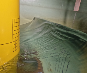
As mentioned previously, intrinsic lateral perturbations of wave breaking are a source of wave impact variability. In nature, residual vortices from the previous wave breaking, wind effect, current and surfactant films that contaminated a water surface (Liu & Duncan Reference Liu and Duncan2003), among other factors, amplify the perturbations on the water surface (figure 1). In most of the research on wave impact variability, water surface disturbances are avoided deliberately to decrease the variability of the results.
The perturbations on the breaking wave curl and breaking wave front (Fox Reference Fox2010).

However, from the engineering point of view it is important to understand and quantify the effect of the perturbations on the pressure and load variabilities.
Here, we investigate the impact pressure, force and impulse variabilities for five variants of focused wave group impacts, and discuss these variabilities as functions of the incident wave shape. The sources of variability are also discussed.
Next, we investigate the impact pressure, force and force impulse variability with the addition of a bottom-mounted perturber that adds transverse ripples on the impacting wave front. After correcting for the change in wave front shape from reflection, we are able to quantify the effect of the lateral disturbances on the pressure variability. Special attention is given to observing air entrainment with associated oscillatory pressure time histories.
The details of our experimental set-up and the mechanism of inducing the perturbations on the breaking wave are described in § 2. The effect of the breaking wave shape topology and perturbation effect is considered in § 3. Slamming force and pressure variabilities for the unperturbed waves are studied in § 4. A frequency analysis for slamming force and pressure is then performed to detect the aeration effect. In § 5, the slamming force and pressure variabilities for the perturbed waves are studied, and the results are compared with those of the unperturbed tests. Results of tests with distinctive frequency content from both the unperturbed and perturbed tests are analysed in § 6 with our observations of the entrainment process. Finally, concluding remarks and suggestions for future work are presented in § 7.
2. Experimental set-up
The experimental tests were carried out following a Froude scaling 1 : 36, in the towing tank of the Center of Marine Technology at NTNU. In figure 2, we present the top and side views of the tank, including the dimensions in the model scale.
Schematic of the present experiments from top and side view, including dimensions of the monopile and the location of experimental set-up components. The figure also shows ten wave gauges (WG) downstream of the cylinder, and two force transducers positioned at the top and bottom of the monopile. The measurements from all sensors are utilized for the analysis in the present paper.

The tank length is 25 m from the zero position of the wavemaker, and the tank width is 2.5 m. The water depth was set to 0.555 m. The wave generation was conducted by a single-piston wavemaker with maximum stroke amplitude 0.2 m. A potentiometer was connected to the wavemaker to record the location of the wavemaker paddle at each test. The desired extreme wave events were designed based on NewWave theory, as detailed in Tromans, Anaturk & Hagemeijer (Reference Tromans, Anaturk and Hagemeijer1991). These events were characterized by a JONSWAP spectrum with significant wave height  $H_{s}=0.21\ {\rm m}$, peak period $T_{p}=2\,{\rm s}$ and peak enhancement factor $\gamma_{JS}=1$ for all conducted tests. The designed wave signal for all tests had duration 100 s, with the focal time set at 50 s. The frequency bandwidth for the JONSWAP spectrum was $[0, 0.25]$ Hz. By changing the focused waves focal points, five different wave breaking shapes were achieved. The first focal point at a distance 0.35 m from the monopile centre was designed such that the wave breaks after the monopile, similar to the slosh impact in Hofland et al. (Reference Hofland, Kaminski and Wolters2011). The other focal points were shifted by 0.1 m relative to the previous focal point towards the wavemaker. The waves were fully broken at the time of impact for the last focal point. Fifty test repetitions of tests were conducted for each focal point, with 120 s resting time between to allow the water surface oscillations to decay. Information about the tests is provided in table 1. A parabolic beach at the end of the tank was fixed to damp the incident waves. The water surface elevation was measured by ten wave gauges (WG) distributed in groups of three, where the middle wave gauge in the first row was 1 m from the monopile centre, and the distance between the first and second, and second and third, rows was constant and equal to 1.0 m. The distance between the wave gauges on each row was constant and equal to 0.8 m. A single wave gauge was placed at distance 3 m from the wavemaker to measure the wave elevation close to the wavemaker. The sampling frequency of the potentiometer and wave gauges was 200 Hz. Water leakage from the tank to the area behind the wavemaker was observed during the experiments. To solve this problem, a pump system was used to transfer the water back to the tank, which caused a periodic change in the water level by a few millimetres.
Test conditions for the unperturbed and perturbed tests, for five focal points,  $n=1,\ldots,5$. The parameters are given in the 1 : 36 scale.

A monopile with diameter 0.3 m, and length 1.2 m was located at distance 15.275 m from the wavemaker. The monopile was made of aluminium, and had a hollow structure and shell thickness 0.01 m (see figure 2).
The two ends of the monopile were sealed to avoid water leaking inside it. Based on knowledge from earlier tests (Bredmose et al. Reference Bredmose2016), two force transducers were used to measure the force on the monopile, mounted at its top and bottom (figure 3) to increase the natural frequency of the system. Sixteen pressure sensors and five accelerometers were used to measure pressure and acceleration on the monopile. The pressure sensors were mounted at three different heights, with the lowest 0.157 m above the still-water level. These sensors were screwed into pre-drilled holes in the cylinder shell and mounted flush with the surface. More detail about the pressure sensors is provided in figure 3. The sampling frequency of these sensors was  $f_s=9600 \, \mbox {Hz}$. A long transverse beam was clamped to rails at the two sides of the tank to fix the top transducer. We will show later that due to the vibrations of the connections at the top platform, some oscillations with a frequency smaller than 100 Hz affect the force transducer outputs.
The location of the sixteen pressure sensors, five accelerometers and two force transducers mounted on the monopile.

The pair of vortices formed during wave breaking is identified as a source of lateral perturbation on the wave crest surface. In the laboratory, these perturbations have a small scale for a single extreme wave; however, in nature, the ambient disturbance also perturbs the water surface, making the lateral perturbation on the wave front more pronounced.
To induce a controlled perturbation of the wave front in the laboratory, and exaggerate the scale of the perturbation on the wave surface in the laboratory, we designed and mounted a mechanical perturber made of thin horizontal wires in front of the monopile along the wave propagation direction (figure 4a). In the presence of the perturber, the water particles flow around the wires, generating vortices parallel to the wave propagation direction to evolve on the water surface. Through the orbits in the wave kinematic motion, these vortices end up in the impact zone (figure 4b). Narayanaswamy & Dalrymple (Reference Narayanaswamy and Dalrymple2002) observed that independently of the wave height and period, the typical width of the perturbation in their experiments was about 0.02–0.03 m, at full scale. Based on that, we used five parallel aluminum wires with diameter 0.0025 m and a constant distance 0.03 m to generate the perturbations. The length and height of the perturber were 0.42 m, and 0.49 m, respectively, and were chosen to ensure that the perturbations were introduced on the wave front at the instant of impact. The wire diameter was chosen as thin as possible to avoid blockage, yet stiff enough to avoid vibration. Some vibration, though, did occur in our tests. A perturber variant made of five thin vertical plates was also tried. This version, however, created a more pronounced vibration and water blockage effect. Selected snapshots of a wave passing through the perturber are shown in figure 5. The ripples on the water surface are the perturbations that form on the wave front surface, and they move toward the wave crest as the wave progresses towards the monopile.
(a) The mechanical perturber with five rods, top view. The support weights are removed. (b) Schematic of the perturber interacting with the incoming wave.

The induction of perturbation by the mechanical perturber and the wave surface: (a)  $t_0$, (b) $t_0+3\,\Delta t$, (c) $t_0+8\,\Delta t$.

A mass of approximately 10 kg was attached to the wooden stand to keep the perturber submerged and fixed at its location. The perturber was located at distance 0.2 m from the monopile centre, and its highest point was 0.03 m below the still-water level. Although the blockage from the perturber rods was small, blockage at the bed occurred due to the perturber's wooden support structure. The structure is shown in figure 4(a), and had height 0.035 m. This change in the bed topology affects the incident waves for the perturbed tests. Using potential flow theory, we estimate that the perturbed tests have a  $5\,\%$ lower wave height than unperturbed tests. For this reason, the comparative analysis of unperturbed and perturbed impacts is conducted based on a regrouping conditional to the wave height and slope at the last wave gauge. More details about the reflection caused by the perturber support are provided in Appendix A.
3. Breaking wave topology
The wave impact on an object is often characterized by the shape of the breaking wave before the impact. Adopted from Hattori et al. (Reference Hattori, Arami and Yui1994) and Hofland et al. (Reference Hofland, Kaminski and Wolters2011) for the impact on a vertical wall, five different slamming wave shapes are sketched in figure 6. These wave shapes are representative of the slamming events generated by the five different focal points chosen in this work. The criterion for the five impacts is the relative positioning between the run-up jet and the overturning wave front.
Schematic of wave front shapes for focal points  $f_1$ to $f_5$ for the impact on the wall.

Figure 6(a) presents the wave shape of the slosh impact, where the run-up jet emerges before the arrival of the wave front, such that no direct wave front impact occurs. The wave shape in figure 6(b) is attributed to the flip-through impact. For this type of impact, the run-up jet and wave front collapse towards a common impact point. Just at impact, the run-up jet flips through the gap between the front and the wall such that no direct impact from the wall occurs (Cooker & Peregrine Reference Cooker and Peregrine1991; Peregrine Reference Peregrine2003). Hattori et al. (Reference Hattori, Arami and Yui1994) discussed that for some flip-through impacts, a single small air pocket may be entrapped, which causes a large impulsive local pressure on the wall. We adopt a convention of no air pocket, and define the regime of a small air gap between the crest and trough at impact as an  $\varOmega$ impact (see figure 6c). This name is chosen because of the similarity of the shape of the wave front to the shape of the Greek letter $\varOmega$. Hofland et al. (Reference Hofland, Kaminski and Wolters2011) indicated small aeration and large slamming pressure scatter for a wave shape similar to the $\varOmega$ impact. This type of impact is generally known to create the largest slamming pressures for wall impacts; see e.g. Bredmose, Peregrine & Bullock (Reference Bredmose, Peregrine and Bullock2009), who conducted a numerical study with a similar set of wave front shapes.
Figure 6(d) shows the wave shape of the overturning impact. Bullock et al. (Reference Bullock, Obhrai, Peregrine and Bredmose2007) characterized this impact by large air pockets and oscillatory pressure due to the air compression and expansion within the trapped air. Figure 6(e) presents the wave shape of a broken-wave impact, where the wave is broken and aerated when it hits the wall, i.e. the plunging jet has hit the free surface before impact at the wall (Hofland et al. Reference Hofland, Kaminski and Wolters2011). We denote the impacts associated with the five focal points by  $f_1$, $f_2$, $f_3$, $f_4$ and $f_5$ in the following.
For the impact on the monopile, five different wave breaking shapes analogous to the ones presented for the vertical wall, and shown in figure 6, were achieved by tuning the focused wave group focal points. The typical breaking wave shape corresponding to each focal point in the experiments is shown in figure 7 for the unperturbed tests, and in figure 8 for the perturbed ones. The snapshots are captured when the wave run-up jet line is approximately 0.02 m below the bottom row of pressure sensors.
The breaking wave front shapes for  $f_1$ to $f_5$ for the unperturbed waves, where the time difference between each snapshot is $6\,\Delta t$, with $\Delta t = 0.024\ {\rm s}$: (a,f,k) $f_1$, (b,g,l) $f_2$, (c,h,m) $f_3$, (d,i,n) $f_4$, (e,j,o) $f_5$.

The breaking wave front shapes for  $f_1$ to $f_5$ for the perturbed waves, where the time difference between each snapshot is $6\,\Delta t$, with $\Delta t = 0.024\ {\rm s}$: (a,f,k) $f_1$, (b,g,l) $f_2$, (c,h,m) $f_3$, (d,i,n) $f_4$, (e,j,o) $f_5$.

For  $f_1$, the focal point location is closest to the monopile. The breaking wave crest horizontal velocity is lower than the wave run-up jet vertical velocity, which results in the wave run-up jet covering the monopile surface before the wave crest reaches it, similar to the slosh impact on the wall. By shifting the focal point by 0.1 m farther from the monopile, a flip-through impact on the monopile front is achieved. Thus in $f_2$, the wave crest gains higher velocity, therefore it encounters the monopile surface almost simultaneously with the run-up jet. We observed that the difference between the wave shape of some tests in $f_2$ and $f_1$ was marginal.
For  $f_3$, the wave front hits the monopile in the vicinity of the top row of pressure sensors first, then the wave run-up jet encloses the wave roller. In this case, the formation of a few air bubbles is possible. The wave impact in $f_3$ is characterized as an $\varOmega$ impact.
The wave overturns and plunges onto the monopile for  $f_4$. The impact zone is usually close to the middle row of the pressure sensors, and in the vicinity of it, we observed noticeable air entrainment for some of the tests. For a similar wave impact on a wall, Hattori et al. (Reference Hattori, Arami and Yui1994) also described a wide cloud of air bubbles inside the water close to the impact zone. They showed that the large air bubbles inside the water had a cushioning effect, reducing the slamming pressures on the wall. Further, they referred to pressure oscillations produced by the entrapped air bubbles.
Finally, for  $f_5$, the wave is fully broken when it hits the monopile. In this case, the pressure sensors may be exposed to the water jets created after the wave breaks from the surface. Therefore, the pressure is expected to be more scattered in time and space compared to other focal points. For a fully broken wave impacting a wall, Mai et al. (Reference Mai, Mai, Raby and Greaves2019) showed that the aeration effect could be smaller than for the overturning impact; however, if the distance where the wave breaks from the wall is small, some air bubbles may be present and cause pressure oscillations.
4. Wave impact variability for the unperturbed tests
We first analyse the impulse, force and pressure variabilities for the unperturbed wave impacts. Even for the 50 repetitions of nominally identical impacts, a notable variability was observed. We therefore start with a categorization of the sources that can affect the incident wave profile. The sources found to possibly affect the global shapes of waves in our experiments are:
(i) variability in the wavemaker displacement history,
(ii) water depth variation between tests,
(iii) wave breaking close to the wavemaker,
(iv) residual water motion from the previous test.
By assessing the time series of wavemaker displacement and velocity, a negligible 0.2 % variation in the maximum displacement and velocity of the wavemaker was identified. This variation is considered to have a minor impact on the overall variability of the results. The pump system's water transfer resulted in a gradual 6 mm variation in water depth every half-hour. Additionally, early wave breaking near the wavemaker and the presence of residual waves significantly influenced the repeatability of wave shape. We believe that these three factors contributed collectively to the variability in results. This section begins by evaluating the cumulative effects of these factors on both wave height and slope. This analysis is crucial for comprehending the sensitivity of the impact to variations in the overall shapes of breaking waves.
4.1. Assessment of incident wave variability
During our experiments, shortly downstream of the wavemaker, we noticed a slight spilling wave breaking, due to the high steepness of the generated waves close to the wavemaker.
The wave gauge (WG) data are analysed to evaluate the variation introduced by all the described sources of variability. Two parameters are chosen for this purpose: the focused wave height  $H$, and the rate of change of the water surface elevation $\eta _t$. We define the wave height as the distance between the focused wave crest height and the focused wave trough. These parameters are illustrated in figure 9. The non-dimensional maximum wave height $\tilde {H}=H/H_s$, and the non-dimensional wave slope $\tilde {\epsilon }=\eta _{t_{max}}(T_p/H_s)$, for WG9, WG6, WG3 and WG1 for all the focal points are presented in figure 10. By qualitative comparison of the plots, we can recognize that the variation at WG1 and WG9 is more pronounced than at the other gauges. For WG1, the variability is mainly due to the wave breaking early close to the wavemaker. However, farther away from the wavemaker, the wave height and slope variability are noticeably reduced; see e.g. WG3.
Definitions of the wave height and the wave slope. The horizontal and vertical axes are, respectively, non-dimensionalized by  $T_p$ and $H_s$.

The distribution of the maximum wave height and wave slope for all the unperturbed waves in  $f_1$ to $f_5$.

In order to assess the variability of the focused wave crest shape, we calculate and present the mean wave height and mean wave slope, and their coefficient of variation (CV), in table 2. The CV is a measure that helps us to understand the relative variability in a dataset, and it is determined by dividing the standard deviation of a quantity by its mean.
Statistical information concerning the wave height and wave slope for each focal point, where  $\tilde {\epsilon }=\eta _{t_{max}} T_p/H_s$ and $\tilde {H}=H/H_s$.

For WG3, we observe that wave slope and wave height variability are lower compared to measurements at WG1. Specifically, the CV for wave height is less than 0.9 % at every focal point. The CV of wave slope is approximately 3 %, indicating that wave slope is more sensitive to disruptions caused by early wave breaking or residual waves. As the focused wave approaches the monopile, the results at WG9 show that there is an increase in variability in both wave height and slope. This higher variability can be attributed to the wave crest's sensitivity to upstream conditions, particularly when it nears the point of breaking. In WG9, the CV for wave height spans from 1.4 % to 2.1 % across all focal points. Some studies, such as that by Marzeddu et al. (Reference Marzeddu, Oliveira, Gironella and Sánchez-Arcilla2017), may consider this variation in wave crest height to be negligible. However, the variability in wave impact force is not only determined by breaking wave height; it is also influenced by the shape of the breaking wave. Therefore, we consider it essential to take into account variations in wave slope as an important parameter for understanding the wave impact variability.
Based on measurements taken by WG9, the CV for wave slope ranges from 10.5 % to 16.8 % at all focal points, significantly higher than the variability in wave height. While wave slope is not the only parameter defining the shape of breaking waves, in this context, it sheds light on the factors contributing to the variation, resulting largely from changes in the timing and location of wave breaking during each test.
4.2. Force variability
The variability of the slamming force on the monopile is now assessed for the nominally identical waves for each of the five focal points. In figure 11(a), the 50 force time series for each focal point are presented. The time axis representing the slamming duration is normalized with  $V_p/D$, where $V_p=\omega _p/k_p$. Here, $\omega _p$ and $k_p$ denote the peak angular frequency and wavenumber, respectively, derived from the linear dispersion relation. In general, the force variability is largest in the slamming part of the force time series; this area is highlighted with a darker colour. The non-slamming part of the force time series is shown with a lighter colour, and it can be seen that regardless of the focal point, it shows high repeatability in general. To study the slamming force variability in detail, the slamming force time series are presented separately in figure 11(b), for 0.05 s before and after the slamming force peak. The mean of the peaks of the slamming forces (referred to as mean slamming force in the following) is shown by an arrow for each focal point.
(a) The force time series of 50 test repetitions for five focal points. The slamming part of the force time series that has the highest variability is shown in black, while the rest is shown in grey. (b) The slamming force time series for each focal point. The arrow indicates the mean of the peaks of the slamming forces for each focal point. The time axis is normalized using two parameters:  $V_p$, defined as the ratio of the peak angular frequency to the peak wavenumber, and $D$, which represents the cylinder diameter.

The mean slamming force from  $f_1$ to $f_3$ does not follow a specific trend; however, from $f_3$ to $f_5$, it decreases. The mean slamming force for $f_1$ is higher than for $f_2$, and marginally lower than for $f_3$. The trend for $f_1$ to $f_3$ contradicts what Wienke, Sparboom & Oumeraci (Reference Wienke, Sparboom and Oumeraci2001) and Bredmose et al. (Reference Bredmose, Peregrine and Bullock2009) found for the slamming force on the monopile and wall, respectively. They demonstrated that the largest slamming force on the monopile is associated with the waves with a developed breaking shape, i.e. similar to $\varOmega$, and that the slosh and overturning impacts cause a smaller slamming force. The evaluation of slamming force peak variability shows a CV for $f_1$ and $f_2$ of 10 % and 12.1 %, respectively. For context, the CV for all other focal points is below 6.2 %. The higher variability of the peaks of the slamming forces for $f_1$ and $f_2$ is considered as the reason for the not-in-agreement mean slamming force development compared to what Wienke et al. (Reference Wienke, Sparboom and Oumeraci2001) and Bredmose et al. (Reference Bredmose, Peregrine and Bullock2009) found.
For  $f_3$, the mean slamming force is the largest among all focal points. Additional to the topology of the $\varOmega$ impact, the large slamming forces can be enhanced by the small air bubbles entrained during the impact. These bubbles distribute the high pressure associated with the impact shock wave over the entire impact zone (Bredmose et al. Reference Bredmose, Peregrine and Bullock2009), yielding a larger integral of pressure and force. The slamming force decreases for $f_4$ and $f_5$, respectively. For these two focal points, the wave plunges. This type of wave breaking does not impose a single large instantaneous force on the monopile. Rather, because of the more complex shape of the breaking wave, multiple slamming peaks, primarily from the breaking tongue and the water jets impact, can be observed.
The variation of the slamming force peak generally decreases from  $f_1$ to $f_5$; however, it is not necessarily the case from one focal point to another. As described, the largest slamming force variation is seen for $f_1$ and $f_2$. By studying specific tests from $f_1$ and $f_2$, it can be seen that the slamming force increases noticeably with the transition in wave shape from slosh to flip-through or $\varOmega$ impact. Given that the difference between the wave shapes of the slosh and flip-through impacts is often marginal, the slamming force becomes remarkably sensitive to any variation in the wave height and slope. The slamming force peak variability decreases after the wave breaks. However, despite the smaller variability, we should acknowledge that for the overturning and broken wave impact in $f_4$ and $f_5$, the instants of the slamming force peaks and the numbers of slamming force peaks are all highly stochastic.
As the presented analysis reveals, wave height and slope variation strongly affect the slamming force. The slamming force variability can be reduced by grouping the forces according to  $\tilde {H}$ and $\tilde {\epsilon }$. To apply grouping, the maximum wave height versus the maximum wave slope of all tests at WG9 are plotted in figure 12. The slamming force peak of each test is also shown, and the greyscale bar indicates the force magnitude. All the parameters are normalized by min–max normalization. To isolate similar waves, we defined some circles within the scattered data in which the CV of the wave height and the wave slope cannot exceed 2.5 % after normalization (red circles in figure 12). The centres of the circles are chosen such that we can fulfil the ${\rm CV}=2.5\,\%$ criterion in each group. In total, five groups are defined, namely $g_1$ to $g_5$, with ten test repetitions inside each group. The breaking wave shape, and correspondingly the wave impact, still vary from test to test inside each group. The typical wave impact for $g_1$ and $g_2$ is of type slosh impact; for the tests in $g_3$ and some tests in $g_4$, the impact type is flip-through; and for some tests in $g_4$ and all the tests in $g_5$, the impact is of type $\varOmega$. For normalized $\hat {H}_{max}>0.5$ and $\hat {\epsilon }>0.175$, the data are overly scattered, and the various criteria for clustering them could not be satisfied. These scattered data correspond mostly to the overturning and fully broken waves.
The data illustrate the maximum slamming force recorded in all test cases across different focal points. Five groups of tests are shown, with red circles where efforts were made to minimize wave height and slope. The axes and greyscale have been normalized for consistency.

The slamming force time series of the regrouped tests are shown in figure 13. The mean slamming force increases from  $g_1$ to $g_5$. Wienke & Oumeraci (Reference Wienke and Oumeraci2005) found the same trend for the slamming force of waves with the same shape as those for $g_1$ to $g_5$; the same trend was also found by Bredmose et al. (Reference Bredmose, Peregrine and Bullock2009) for impacts on a wall. The slamming force peak variability is significantly reduced inside each group, and the CV of the slamming force peak is between 2.1 % and 4.5 % for all of the groups (table 3). The slamming force peak variability has an increasing trend from $g_1$ to $g_5$, indicating the higher sensitivity of the flip-through and $\varOmega$ impacts on the wave shape variation. This remarkable reduction in force variability compared to the results for $f_1$ and $f_2$ demonstrates the high correlation of the slamming force variability with wave height and slope variability.
Time series of the slamming force of the regrouped tests.

Comparison of the slamming force, pressure, impulse mean and variability. Here, UP and P refer to unperturbed and perturbed tests,  $\tilde {I}$ is the non-dimensional impulse, $\tilde {F}_{max}$ is the non-dimensional maximum force, $\tilde {P}_{max_{L}}$ is the non-dimensional maximum pressure from the left sensor in the top row (S2), and $\tilde {P}_{max_{R}}$ is the non-dimensional maximum pressure from the right sensor in the top row (S3).

The impulse variation for each group is shown in figure 14. The impulse is calculated by integrating the slamming force time series in the time span presented in figure 13. The mean impulse values are generally very similar in all groups. Thus the impulse is less sensitive to wave height and shape variability. The constant behaviour trend for the mean impulse is due to the time integration that flattens out the high force values within a short time span of slamming. The CV values of impulses are very similar in all groups. As shown in table 3, the CV of impulse for  $g_1$ is about 0.7 %; for $g_5$, it is about 1 %, which is smaller than the CV of the slamming force in $g_1$ and $g_5$, respectively.
The slamming force impulse variation for each group for the unperturbed tests.

Some oscillations are observed in all the time series, and their amplitude increases from  $g_1$ to $g_5$. To identify the source of these oscillations, the power spectral density (PSD) of the slamming force was calculated for each test, and the group averages are presented in figure 15. The natural frequencies of the monopile as determined from acceleration data are shown with dashed lines.
The averaged PSD of slamming force for all groups:  $g_1$ in pine green, $g_2$ in blue, $g_3$ in yellow, $g_4$ in red, and $g_5$ in lime green. The natural frequencies of the set-up are shown with dashed lines. The electrical current frequency and its harmonics, from 1st H to 4th H, are indicated.

All the peaks below 200 Hz are related to the harmonics of the electrical current or the natural frequencies of the set-up. The electrical current supply is 50 Hz, and the harmonics of this frequency are indicated in figure 15 up to the fourth harmonic, i.e. 200 Hz. The relatively large amplitude oscillations seen in the slamming force time series in figure 13 after the slamming peak are due to the excitation of the structural mode at frequency 110 Hz. Other peaks are visible in figure 15 due to the excitation of higher natural frequencies. A frequency range is highlighted in grey, where the PSD of  $g_4$ and $g_5$ shows high energy between two natural frequencies. Due to the artificial effects brought on by the windowing process used to compute the power spectra, and the similarity of these frequencies to the natural frequencies of the set-up, it is difficult to define the main driver of the oscillations related to these frequencies. However, given that these frequencies are mainly recognizable in the PSD of $g_4$ and $g_5$, and their impact type is mainly flip-trough or $\varOmega$, we consider the air bubble oscillations as a possible cause of the excitation of these frequencies. We will return to the observation of air bubbles in § 6.
4.3. Pressure variability
Bullock et al. (Reference Bullock, Obhrai, Peregrine and Bredmose2007) showed that the slamming pressure variability is more significant than the slamming force variability for wave impacts on a wall. The breaking wave front disturbances can cause non-uniform impacts with respect to the  $xz$-plane, resulting in variation in the location of the maximum pressure. The interaction of the breaking wave crest and wave trough jet on the monopile creates water jets that may hit the monopile at the location of the pressure sensors, causing a large value in the pressure signals. Further, aeration also affects the wave impact pressure distribution on the monopile, which can cause variation in the pressure detected by the sensors. In figure 16, the pressure variability is evaluated by data from a pair of pressure sensors closest to the middle of the monopile at three different heights. The bars show the mean plus/minus one standard deviation of the peaks of the slamming pressures, and the markers indicate the pressure peak value for each test. It can be observed that the mean slamming pressure increases from the bottom to the top row of the pressure sensors. With the current arrangement of the pressure sensors, the highest pressures are detected at the point where the wave crest tip impacts the monopile. The left and right pressure sensors show a similar mean slamming pressure, which implies that the transfer of wave momentum to the area in the centre of the monopile surface is even. The variation in slamming pressure increases from bottom to top. From the video recordings, we have observed that small variations in the wave crest shape or local disturbances along the wave crest tip may be the reason for the higher slamming pressure variability on the top row.
Distribution and variation of the slamming pressure at the area in the middle of the monopile. Sensors to the left of the middle axis are shown in black; sensors to the right of the middle axis are shown in orange.

The mean slamming pressure peak and slamming pressure variability also increase from  $g_1$ to $g_5$. For $g_1$ (sloshing impact), since the wave crest does not hit the monopile directly, the variations in the wave shape are of lower relevance. Therefore, the repeatability of the slamming pressure peak is higher than for the other groups, and the CV is approximately 14 %. The slamming pressure peaks for $g_4$ and $g_5$ (flip-through and $\varOmega$ impact) show substantial variability due to the interaction between the wave crest tip and wave trough, air entrainment, and variations in the shape of the wave crest tip. For $g_5$ (top row), the CV of the peaks of the slamming pressures is 29 % for the left sensor, and 32 % for the right sensor. Due to the limited number of pressure sensors, the pressures detected by the top row of the pressure sensors are not necessarily the largest pressures that the monopile experiences during the impact, and the mean and variability can be larger in the higher locations at the impact zone.
The temporal development of the mean slamming pressure for each sensor in each group is investigated in figure 17. For the sake of conciseness, the pressure time series for  $g_1$ are not shown, since their trends are similar to the pressure time series trends for $g_2$, although smaller magnitude-wise. It can be seen that the pressure peak build-up is more gradual for $g_2$ and $g_3$, while for $g_4$ and $g_5$ (flip-through and $\varOmega$ impact, respectively), it is more abrupt. The left and right sensors, except for $g_5$ (top row), generally show very similar time series pre- and post-slamming pressure peaks, which indicates that the wave trough jet, or wave front jets, do not cause uneven pressure distribution at the middle of the monopile surface for the averaged time series. For $g_5$, before the pressure peak, oscillations can be seen in the pressure time series of sensor S2. The same oscillations, with a relatively smaller amplitude, exist in the pressure time series of S3. Specific pressure time series recorded multiple pressure peaks, presumably because the water jet hits the monopile before the main front of the breaking wave impacts it. Since this figure shows the mean pressure time series, the peaks are averaged.
Mean pressure time series for  $g_2$ to $g_5$. The time series for each pressure sensor is zero-levelled by the time of the slamming force peak. The left sensor is given by a solid black line; the right sensor is given by a dashed orange line.

In the pressure time series of all sensors in  $g_4$ and $g_5$, oscillations of various frequencies can be found, most notably for $0< t V_p/D<0.05$. The amplitude of the oscillations increases from the bottom to the top row of sensors. To understand the source of the oscillations, the power spectra of the pressure time series are calculated, and their average is presented in figure 18. The natural frequencies of the set-up are also shown with dashed lines. For $g_2$ and $g_3$, the mean PSD is almost flat all over the spectrum. Frequency contents in the range $480\ {\rm Hz}< f<1440\ {\rm Hz}$ can be observed for the sensors in the middle and top rows. These frequencies, however, are low in energy and are caused mainly by noise. For $g_4$ and $g_5$, the peaks in the PSD are more noticeable. Most of the peaks are located at the natural frequencies, indicating that the oscillations in the pressure time series are due mainly to the monopile vibrations, which change the pressure. At approximately 960 Hz, a flat region with high energy content is observed in the PSD of the sensors in the top row for $g_5$. This frequency is close to the peak in the force PSD at approximately 1000 Hz in figure 15. A few uncertainties come along with determining the source of the high energy content at 960 Hz, given that it is close to the natural frequency of the system. However, the fact that this frequency strongly appeared in the PSD of only the pressure sensors in the top row suggests that it may be related to oscillations caused by air bubbles.
The mean PSD of slamming pressure for  $g_2$ to $g_5$. The left sensor is given by a solid black line; the right sensor is given by a dashed orange line.

5. Assessment of perturbed wave elevation and impact variability
We now proceed with the results for the perturbed wave impacts, obtained by repeating the 250 perturbed tests with the perturber present in the basin.
5.1. Assessment of incident wave variability
As we described before, several factors could cause variations in the breaking wave shape for the nominally identical waves in laboratory conditions. Further, the presence of a mechanical perturber changes the wave front topology. First, the perturber alters the wave front shape by inducing both ordered vortical structures and turbulent eddies created when waves pass through the perturber's wires. Second, the perturber's support structure causes a depth discontinuity that includes wave diffraction. The combination of both effects changes the breaking wave front global and local shapes.
The variation of the slamming force peak is illustrated by the mean plus/minus one standard deviation of the peaks of the slamming forces in figure 19. The unperturbed results are also provided for comparison. The mean slamming force of the perturbed tests for  $f_1$– $f_3$ is noticeably smaller than for the unperturbed tests. As shown in figure 20, the wave crest height for the perturbed tests is smaller than for unperturbed, which is considered to be the main reason for the smaller slamming force observed in the unperturbed tests. For $f_4$ and $f_5$, the mean slamming forces are more similar. For both focal points, the waves in the perturbed and unperturbed tests plunge onto the monopile or fully break immediately before it. Therefore, the diffraction effect does not stand out.
The mean plus/minus one standard deviation of maximum slamming force for all the perturbed and unperturbed tests. The circular markers represent the maximum slamming force value for each test. Perturbed is shown in red, unperturbed in black.

(a) Probability density estimation of the unperturbed and perturbed tests: unperturbed with a black dashed line, perturbed with a solid red line. (b) Scatter plot of the normalized wave height and wave slope for the unperturbed and perturbed tests. The circles show the location of each group; unperturbed shown with grey dots, perturbed with red triangles.

For  $f_1$ and $f_2$, the slamming force peak variability of the perturbed tests is lower than for unperturbed. Given that perturbation increases the stochasticity of the wave front shape, and consequently the slamming force, we expect to see higher variability for the perturbed tests. This suggested that the presence of the perturber led to changes not only laterally along the wave front but also to the shape of the impacting wave. Figure 19 confirms that this is the case. To understand the overall effect of the mechanical perturber on the waves, we compared the probability density of the wave height and the wave slope in figure 20(a). The figure shows that for the majority of the perturbed tests, the wave height is $\hat {H}<0.6$ and the wave slope is $\hat {\epsilon }<0.4$, whereas for the unperturbed tests, the distribution is extended to higher and steeper waves, for which $\hat {H}<0.9$ and $\hat {\epsilon }<0.6$, respectively. This difference between the unperturbed and perturbed waves shows that the diffraction caused by the perturber reduces the wave height and the wave slope. More information on the diffraction effect is provided in Appendix A. Hence, since the waves and impacts cannot be compared directly between the perturbed and unperturbed waves, we decided to regroup them following the same method as for the unperturbed test, and compare the variability throughout the regroup sequence. As shown in figure 20(b), in total, four circles (groups) were defined, in which ten tests from each perturbed and unperturbed set were collected. Extending the number of the groups to five was not possible since fewer than ten perturbed tests would be inside $g_{5}$. By visually inspecting the breaking wave shapes in all tests within each group, we identified slosh impact in the majority of tests in $g_{1}$. A combination of slosh and occasional flip-through is shown in $g_{2}$, while $g_{3}$ is characterized mainly by flip-through. In $g_{4}$, the prevailing impact type is flip-through, with occasional occurrences of $\varOmega$ impact.
The slamming force time series and statistics about the slamming force variability for the regrouped tests for both perturbed and unperturbed wave tests are provided in figure 21. After regrouping, the mean slamming force of the perturbed and unperturbed tests generally becomes more similar. For  $g_1$ to $g_4$, the mean force of the unperturbed test is approximately 4 %–7 % higher than the perturbed one. This difference is attributed mainly to the effects of the perturbations. Compared to an unperturbed impact, where the wave front surface is smooth, the irregularities and asymmetries imposed by the perturbations may prevent the sudden transfer of the slamming force onto the cylinder, lowering the magnitude of the slamming peak and elongating the rise-up time. The slamming force variability of the perturbed tests is higher than the unperturbed ones in all groups. For $g_1$– $g_3$, the CV of the slamming force of the perturbed tests is approximately 1.0 % higher than for the unperturbed ones. However, for $g_4$, this difference is more noticeable, with the CV increasing from 2.1 % to 5.7 %. As discussed in Appendix A, the diffraction has a minor effect on the wave crest height and slope variation; therefore, higher variations of the slamming force for the perturbed tests are related mainly to the perturbations induced by the wires of the perturber.
Time series of the slamming force for the regrouped tests. Perturbed is shown in red, unperturbed in black.

The impulse variability for each group is shown in figure 22. The results for the unperturbed tests are also presented in the figure for comparison. Like the unperturbed tests, the mean impulses of the perturbed tests in all groups are very similar. The CV of impulse for the perturbed tests for  $g_1$ and $g_2$ shows less variability than for the unperturbed tests, while for $g_3$ and $g_4$, the variability of the perturbed tests is higher. However, generally, the CV is approximately 1 % for all groups. These results suggest that the perturbations have a small effect on the impulse variability.
The slamming force impulse variation for each group of tests. Perturbed is shown in red, unperturbed in black.

The PSD plots of the slamming force time series for the perturbed test groups are shown in figure 23. Most PSD peaks below 400 Hz are related to the harmonics of the electrical current or the system natural frequencies. For  $g_3$ and $g_4$, two peaks are highlighted in the figure. The first peak, at 525 Hz, is very close to the system natural frequency, so we consider its source to be on the monopile vibrations. The second peak, at 580 Hz, does not correspond to a natural frequency. Although we cannot indicate its exact origin without considering the pressure time series at different locations on the monopile surface, we consider it related to air bubble oscillations. For the rest of the spectra, the PSD plots of all groups are similar, and in general, fewer natural frequencies are excited compared to the unperturbed cases.
The averaged PSD of slamming force for the perturbed tests for all groups:  $g_1$ in pine green, $g_2$ in blue, $g_3$ in yellow, $g_4$ in red.

5.2. Pressure variability
The effect of the perturbations on the mean slamming pressure and the slamming pressure variability is presented in figure 24 together with the results from the unperturbed tests. The general trend for the mean slamming pressure of the perturbed tests is similar to that of the unperturbed ones. However, the variation of the slamming pressure for the perturbed tests is larger than for the unperturbed tests, especially for the sensors on the top row. The variability of the slamming pressure increases from  $g_1$ to $g_4$. For $g_1$ and $g_2$, the impact is mainly of type slosh. The wave trough jet covers the monopile surface for the slosh impact, and the perturbed wave crest does not impact the monopile directly. Therefore, the pressure sensors cannot detect the effect of the perturbation directly. This process is illustrated in figure 25, where three snapshots of a perturbed wave of $g_2$ impacting the monopile are shown. As the wave progresses towards the monopile, a jet is formed along the cylinder front wall (see figure 25c). This jet covers the pressure sensors and prevents the direct contact of the wave crest with the monopile surface. However, the variation introduced to the wave kinematics by the perturbations still affects the slamming pressure. In $g_1$, the variation of the perturbed tests is approximately 10 % higher than that of the unperturbed ones. For $g_4$, the difference between the slamming pressure variability of the perturbed and unperturbed waves is considerable. In this case, the pressure sensors are exposed to the laterally perturbed wave crest. As a result, the perturbation effect on the slamming pressure variability is more significant relative to the unperturbed case. Further, the mean and variation of the slamming pressure peaks for the middle sensors S2 and S3 are different, which means that the perturbations cause a lateral variability of non-uniform impact. The non-uniform impact enhances the uncertainty regarding the maximum slamming pressure value and its location. The CV values of the S2 and S3 sensors are 47 % and 57 %, respectively. These CV values are noticeably higher than those seen for the unperturbed tests.
Comparison of pressure variability of the perturbed (P) and unperturbed (UP) tests for all groups using data from the sensors at the middle of the monopile.

Snapshots of the slosh impact for a perturbed test: (a)  $t_{0}$, (b) $t_{0} + 1\,\Delta t$, (c) $t_{0} + 2\,\Delta t$.

In figure 26, we consider the slamming pressure time series of the perturbed tests to investigate any perturbation-related effect. For  $g_1$ to $g_3$, the mean pressure time series of sensors in the same row are similar in terms of trend, peak time instant and peak value. For the pressure sensors in the top row in $g_4$, discrepancies exist between the pressure time series and peak values on the left and right sensors (S2-S3). Additionally, some oscillations are noticeable after the slamming pressure peak. To comprehend the cause of these oscillations, the slamming pressure PSD for $g_4$ was analysed. It was discovered that the natural frequency of the system at 535 Hz is excited. Furthermore, a peak at 780 Hz was identified in the pressure PSD for S2-S3. Since this heightened energy content at 780 Hz was detected exclusively by the pressure sensors on the top row, it is believed that air bubble oscillations could be the source of the excitation at this frequency.
Mean slamming pressure time series of the perturbed tests for  $g_1$ to $g_4$. The time series for each pressure sensor is zero-levelled by the time of the slamming force peak. The left sensor is given by a solid red line; the right sensor is given by a blue dashed line.

5.3. Statistics figures on the variability
We summarize the analysis of the perturbation effects by statistical analysis. For the grouped waves  $g_1$ to $g_5$, the mean and CV of the impulse, slamming pressure and slamming force are provided in table 3 for all the unperturbed and perturbed tests. The mean impulses in all the groups for the perturbed and unperturbed tests are almost identical. Further, the CV of the impulses for most tests is below 1 %. These results support that the impulse has a small sensitivity to the wave variation. The variation of the mean slamming force is higher than for the impulse. The slamming force varies with the wave shape, and by introducing perturbations, the variation increases. The mean slamming force is smaller for the perturbed impacts, but the variability is larger than for the unperturbed impacts. For $g_4$, the slamming force variability of the perturbed impact is more than twice as large as the unperturbed one. The slamming pressure shows high sensitivity to the wave shape and the lateral perturbations, and the pressure variability is more prominent than the slamming force. The mean slamming pressure for the perturbed tests is generally smaller than for the unperturbed ones, except for $g_1$. The slamming pressure variability is, however, larger for the perturbed tests than for the unperturbed ones. We defined the spatial variation of the slamming pressure for a wave impact as the difference between $P_{max_{R}}$ and $P_{max_{L}}$. This spatial variation is higher for the perturbed tests than for the unperturbed ones, which shows that the perturbations increase the stochasticity regarding the location and the value of the maximum slamming pressure. For $g_4$, where the impact is mainly of type flip-through and $\varOmega$, the slamming pressure sensitivity to the perturbation is the highest, and the variation of the perturbed tests is about five times larger than that of the unperturbed ones. While these results show a clear dependency through the groups, it is worth noting that the variability can change significantly if the criteria defined for the variation of the wave height and slope change, or if a different method to generate extreme waves is used.
6. Selected events
Several tests in our experiments showed distinct slamming pressure time series and power spectra. For these tests, we often observed a large slamming pressure magnitude and oscillations in the time series. Some of these oscillations were related to vibration in the set-up, while from PSD analysis, some are also expected to be associated with air bubble oscillations. Most of these tests do not belong to any regrouped tests ( $g_1$ to $g_5$). To identify these tests, we analyse the slamming pressure time series of the unperturbed and perturbed tests spectrally, and we selected the tests that show a higher energy content for some specific frequencies in the PSD. The selected unperturbed and perturbed tests are indicated in figure 27 by $A,B,C,D,E$. In Appendix B, the details about the process of selecting these tests are provided.
Selected events that are considered for analysis; marked in red,  $A,B,C$ correspond to the unperturbed groups, and $D,E$ correspond to the perturbed one.

6.1. Event  $A$
$A$

In figure 28, the slamming pressure time series of event  $A$ from focal point $f_1$ is shown. All the time series are zero-levelled by the time of the slamming force peak. The slamming pressure magnitude detected by the sensors in the top row (S1–S4) is the highest, and it decreases to lower values in the middle and bottom rows. High-frequency oscillations are visible in all of the pressure time series. The magnitude of these oscillations for the sensors in the top row is higher than for the others. The oscillatory behaviour of the pressure time series may resemble the pressure recorded in the case of air bubbles. However, given that all the pressure oscillations are in phase for the sensors in the same column, we believe that the most likely source of the oscillations is dynamic pressure induced by the set-up vibration at a natural frequency.
Unperturbed tests event  $A$: pressure oscillations due to the natural frequency excitation and low aeration.

In figure 29, PSD plots of the pressure time series for all sensors are presented. For the sensors placed farther from the middle of the cylinder (i.e. S5, S11, S1, and S6, and their mirror on the right-hand side), the PSD peak frequencies are mostly at the natural frequencies of the system. For S2 and S3, some peaks with frequencies  $f\approx 370$ Hz, $f\approx 960$ Hz and $f\approx 1061$ Hz can be seen that are not at the natural frequencies, but are close to them. To understand the exact source of these frequencies, more advanced measurement tools and synchronized underwater video recordings with measurements are needed. Nevertheless, we conducted unsynchronized underwater video recordings for random tests for each focal point, and in some of our videos, air bubbles are detected. In figure 30, some snapshots of a wave impact are shown. The snapshots do not belong to the results presented in figure 28; they are just an example case of the bubble formation process for a breaking wave with a similar shape to the test presented here. In figure 30(a), the breaking roller is shown. The middle and bottom rows of the pressure sensors are under water due to the water run-up, and no air bubbles can be seen in their vicinity. Figure 30(b) shows how the wave roller is closed and groups of bubbles formed. In figure 30(c), a bubble close to the top row of pressure sensors is observed, and its size is magnified to ease viewing. Most bubbles go around the monopile driven by the water flow; however, the bubbles in the middle remain for a longer time until they are moved away by advection and buoyancy. The size of the bubbles that affect the pressure data can be estimated by the following equation derived by Minnaert (Reference Minnaert1933):
 \begin{equation} r_b = \frac{1}{\omega_b}\sqrt{\frac{3\gamma P_0}{\rho_0}} . \end{equation}
In this equation,  $\gamma =1.4$ is the adiabatic exponent of compression, $\rho _0$ is the air density, $P_0$ is the atmospheric pressure, and $r_b$ and $\omega _b$ are the radius and natural frequency of the air bubble, respectively. Using (6.1), the frequencies $f\approx 370$ Hz and $f\approx 960$ Hz correspond to bubbles with radius $r_b=0.0113D$ and $r_b=0.0283D$, respectively, where $D$ is the cylinder diameter. The distance between the pressure sensors is approximately $0.0667D$, and based on experimental snapshots, these air bubble sizes are consistent with the estimation based on the equation. Thus we attribute these oscillations to air bubble oscillations.
Unperturbed tests event  $A$: pressure oscillations due to the natural frequency excitation.

Event  $A$: snapshots of small-bubble formation for a low-aeration wave impact. Note that the bubble is magnified. (a) Breaking wave roller. (b) Closed roller, and bubble formation. (c) Bubbles transitioning towards the water surface.

6.2. Event $B$: medium-aeration impact

The effect of the air bubble oscillations is more obvious in some tests from  $f_3$ to $f_5$. The breaking shape associated with these focal points implies air entrainment between the monopile and the wave front or inside the wave roller. Therefore, medium or high aeration can happen, depending on the breaking shape and the wave front interaction with water run-up. The pressure time series for a medium aeration wave impact is shown in figure 31. This test is chosen from the $f_4$ test case. Multiple pressure peaks at different time instants can be seen. The maximum pressure is detected by the sensors in the middle row; however, high pressure is also measured by the bottom row (S11). Oscillations with different frequencies and decay times are seen for all sensors. We attribute most of the high-frequency oscillations to the oscillation of air bubbles of varying sizes in the immediate vicinity or directly on the sensors. Figure 32 presents selected snapshots from a video featuring medium-sized bubbles. Figure 32(a) showcases the breaking wave roller, revealing the intersection of both the wave trough jet and the overturning wave front with the monopile structure. Entrained air inside the wave roller, along with some air bubbles before the roller fully closes, is evident. In figure 32(b), the closed breaking wave roller reveals air bubbles of different sizes covering nearly all the pressure sensors. In figure 32(c), some air bubbles that still cover the pressure sensors in the bottom row can be seen. The time difference between the second and third snapshots is approximately 20 ms or $t V_p/D = 0.1411$, which implies that the air bubbles can affect sensor measurements since the bubbles may persist throughout the full duration of the time series shown. In the videos, we noticed that once the wave impacts the monopile, the bubbles move in a circular pattern. The effect of this motion on the pressure oscillation cannot be comprehended well since underwater video recording was not conducted for every test. However, the low-frequency oscillations (e.g. within a time range $-0.08 \lessapprox tV_p/D \lessapprox 0.03$ for S1 and S2) may be caused by either the transport of bubbles or the oscillation of large air bubbles.
Unperturbed tests event  $B$: pressure oscillations due to the natural frequency excitation and medium aeration.

Event  $B$: snapshots of bubble formation for a medium aeration wave impact. (a) Water and gas mixture by jets shoots up inside the breaking wave roller. (b) Closed roller, and bubble formation. (c) Tube shape bubbles on the pressure sensors area.

The PSD of the pressure time series does not provide comprehensible information due to the short duration of the slamming pressure that causes high energy over the broad range of frequencies. Thus the PSD figure is not provided. From figure 31, the frequency of the pressure time series oscillations for S7 is  $f \approx 1290$ Hz. This frequency is attributed to an air bubble with radius $r_b=0.0083D$.
6.3. Event $C$: high-aeration impact

The last case from the unperturbed tests is chosen due to the transient non-synchronized oscillations and pressure peaks at different time instants, which we consider may be caused by high aeration. Figure 33 shows the slamming pressure time series for a test from  $f_5$. As in the previous case, multiple pressure peaks and frequencies can be observed. However, the slamming pressure peaks are more distributed in time. Since the wave is fully broken when it reaches the monopile, the jet reflects from the water surface after the wave breaking, and the wave front and jet can hit the sensors separately, which can cause several pressure peaks at different times. The analysis of the pressure time series for the sensors in the bottom row shows that the frequency of the oscillations in the range $-0.03 \lessapprox tV_p/D \lessapprox 0.07$ is $f \approx 684.37$ Hz. This frequency can be related to an air bubble with radius $r_b=0.0167D$. A lower frequency oscillation, $f \approx 187.2$ Hz, can be seen for the top and middle row sensors. It is possible that the source of this oscillation is an air bubble oscillation. However, as in the previous case, it is not possible to determine the source of this oscillation with high certainty without knowing more about water kinematics or having an underwater camera recording for each test. An example of a high-aeration wave impact is shown in figure 34. In figure 34(a), it is depicted that when the breaking wave roller closes, due to the interaction of wave trough jets and breaking wave crest, the water jets and air are injected into the water, making a tube shape cloud of air bubbles. This cloud of air bubbles swirls in front of all rows of pressure sensors, and it moves towards the sides, as shown in figure 34(c). We consider the low-frequency oscillations in figure 33, e.g. S9 from the maximum pressure time to approximately $t V_p/D = 0.06$, to be related to the motions of the air bubble cloud.
Unperturbed tests event  $C$: pressure oscillations due to the natural frequency excitation and high aeration.

Snapshots of bubble formation for a high aeration wave impact. (a) Breaking wave roller. (b) Closed roller, and bubble formation. (c) Tube shape bubble structures moving towards the sides.

6.4. Event $D$: perturbed impact with sub-atmospheric pressure

A perturbed impact from  $f_3$ is chosen, and its pressure time series is presented in figure 35. The pressure time series for this case are all in phase, and their peaks descend from the top row to the bottom row. The high-frequency oscillations for S1, S2 and S3 attain sub-atmospheric values, whereas for S4, this oscillation cannot be seen, and instead, a lower-frequency oscillation from $-0.0564< tV_p/D < 0$ is observed. From the pressure time series, we detect that most of the oscillations are due to the excitation of two natural frequencies of the set-up, at $f \approx 528$ Hz and $f \approx 624$ Hz. In figure 36, some snapshots of a video recorded for a perturbed wave impacting the monopile are presented. The perturbation caused by the perturber can be seen in figure 36(a). Figure 36(b) shows the bottom row of the pressure sensors, covered by the wave trough jet. Figure 36(c) shows the closed wave rollers and bubble formation. In this picture, S3 is covered by an air bubble, and the bubbles pass over the rest of the pressure sensors in the top row. Apart from the visibility of the perturbation vortex tubes in the first snapshot, no direct effect of the perturbation on the process of bubble formation can be reported here, except for the probability that the perturbation may prevent the formation of larger bubbles.
Perturbed tests event D: pressure oscillations due to the natural frequency excitation and high aeration.

Snapshots of bubble formation for a low-aeration wave impact. (a) Breaking wave roller. (b) Closed roller, and bubble formation. (c) Bubble structures on the pressure sensors.

6.5. Event $E$: perturbed impact

The last event that we present here, in figure 37, is also from a perturbed impact. This case is selected because of the very large pressure detected by the pressure sensors in the top row. The detected pressure is the highest for S2, and it is 23 % larger than the pressure peak recorded by S3. Large oscillations after the impact are observed and are synchronized in all the time series. Also, a sub-atmospheric pressure is recorded by S1 and S5. The frequency of the oscillations after the pressure peak for all sensors is close to 535 Hz, which is a natural frequency of the set-up.
Perturbed tests event  $E$: pressure oscillations due to the natural frequency excitation and high aeration.

7. Summary and conclusion
We have evaluated the slamming force and pressure variability for monopile wave impacts as a function of the breaking wave shape, and assessed the effect of lateral perturbations on the breaking wave front. Focused wave groups with different focal points were generated to achieve five wave breaking shapes, which were characterized as sloshing, flip-through,  $\varOmega$, overturning and fully broken, inspired from two-dimensional wall impacts. Fifty repetitions for each of the five incident wave groups were made.
Despite the waves being nominally identical for each of the groups, we observed a strong variability for the maximum impact force within the groups. The largest forces were observed for the first two focal points, where also the largest coefficient of variation (CV) for the peak forces of order 10 % was found. Further analysis of the wave gauge signal, however, revealed that even within the groups, the incident wave height and wave slope showed substantial variation. This variation was explained in terms of pre-breaking and residual motion in the basin. The value of the peak impact force was found to vary substantially not only with the incident wave height but also with the maximum rate of change (slope) for the free-surface elevation.
To reduce the variability, tests with similar wave height and slope were selected and gathered into five groups, each with ten repetitions. After regrouping, the variation of the slamming force decreases significantly, and the CV for the force peaks becomes in general less than 5 %. We observed that the mean slamming force peak increases from slosh to  $\varOmega$ impact, qualitatively similar to the findings of Wienke & Oumeraci (Reference Wienke and Oumeraci2005). The mean slamming pressure, which was found to be the largest for the $\varOmega$ impact, behaves similarly to the mean slamming force. The slamming pressure variability is higher than the slamming force variability. The variation was found to be highest for the $\varOmega$ impact, with CV approximately 32 %. For all impact types covered in the groups, the sensors located in the middle of the monopile and farthest from the still-water level (top row of pressure sensors) always detected the highest slamming pressure. The force impulse mean value for all of the groups is similar, and the force impulse variability is approximately 1 %, which conveys that the impulse is significantly less sensitive to wave shape variations.
The effect of lateral perturbations on the wave front was investigated by placing a mechanical perturber in front of the monopile. Although the perturber was intended to induce a lateral variation along the wave front, it was also found to change the incident wave shape. For this reason, the grouping analysis was repeated for the perturbed events, such that the variation through groups with the same incident wave height and slope could be compared. After regrouping, the slamming force variability of the perturbed tests was found to be higher than for the unperturbed ones. This difference is regarded to be associated with the perturbation effect. The slamming pressure variability of the perturbed tests is also notably higher than for the unperturbed ones. For the slosh impact where the wave crest does not impact the monopile surface directly, the CV for the perturbed waves is approximately 20 %, whereas the CV for the unperturbed tests is of the order of 12 %. For the  $\varOmega$ impact, the difference between the CV for the perturbed and unperturbed tests is larger: for the unperturbed waves, the CV is 10 %, and for the perturbed tests, it is 52 %. The impulse mean values for all the impact types were found to be very similar, and the perturbation barely affected the impulse variability. The variation of the impulse is of the order of 1 %.
Some events with special pressure time series and spectra were presented with detailed analysis. Air bubble formation was documented by video footage, which revealed how bubbles are trapped at the lower and upper edges of the collapsing roller against the monopile or by air entrainment during the wave impact process. We show that large slamming pressure with oscillations with positive and negative values after the slamming pressure peak does not necessarily relate to bubbles oscillations. If the structural modes are excited, then the oscillations of the monopile can cause a significant pressure change in water, resulting in oscillatory pressure with positive and negative values even without air bubbles. By analysis of accelerometer measurements, we detected the natural frequencies of the set-up, and identified the vibration-related oscillations. For some tests, air bubble oscillations outside the natural frequencies were detected mainly in focal points 3, 4 and 5. Usually, only one or two sensors picked up the bubble oscillations, and they decayed rapidly. The frequencies of the bubbles that we detected were between 250 Hz and 1100 Hz. Besides the quantification of the impact impulse, force and pressure as a function of wave shape and perturbation, the present investigation thus provides evidence of air bubble formation for monopile impacts.
Acknowledgements
The invaluable assistance of technicians at the Lilletanken laboratory at NTNU is appreciated.
Funding
This research was supported by a PhD grant (A.M.) in relation to the Nordic Offshore Wind Research and Innovation Centre (NOWRIC) at DTU, NTNU and SINTEF.
Declaration of interests
The authors report no conflict of interest.
Appendix A. Analysis of wave reflection
Here, we investigate the mean and variability of the wave height and slope of the perturbed tests. The wave gauge data are analysed to assess the effect of the wave reflection due to the local water depth discontinuity caused by the mechanical perturber support structure.
The maximum wave height and slope measured by wave gauges WG1, WG3, WG6 and WG9 for all focal points for the unperturbed and perturbed tests are presented in figure 38. The mean and standard deviation are provided in table 4. As for the unperturbed tests, in the perturbed tests, the waves close to the wavemaker were slightly breaking (spilling). Due to the pre-breaking, the wave data measured by WG1 is highly scattered. After pre-breaking, as shown in figures 38(f–j), the wave height and slope variability become smaller. However, as the wave progresses towards the monopile and becomes steeper, the wave height and slope variability increase again (figure 38, WG6 and WG9). At the location of WG9, the wave height of the perturbed tests is lower than the unperturbed ones for all the focal points. The lower wave height is most likely associated with the reflection of the wave due to the local water depth discontinuity. The reflection reduces the wave height of the perturbed tests by 1 %–5 %. The CV values of the wave height and slope of the unperturbed and perturbed tests, however, are similar (see table 4), which means that the wave reflection did not noticeably affect the wave height and slope variability. From  $f_1$ to $f_5$, the difference between the CV of wave height for the unperturbed and perturbed waves at WG9 is less than 1 %. For the wave slope, the difference is larger; however, it is normally below approximately 6 %.
The distribution of maximum wave height and wave slope for the unperturbed and perturbed tests at each focal point: unperturbed shown in black, perturbed in red.

The statistical information about the wave height and wave slope of the unperturbed and perturbed waves for each focal point. The mean difference is the variation between the mean wave height (or slope) of the unperturbed and perturbed tests divided by the value of the mean unperturbed tests. Here,  $\Delta \tilde {\epsilon }=(\tilde {\epsilon }_{up}-\tilde {\epsilon }_{p})/ \tilde {\epsilon }_{up}$ and $\Delta \tilde {H}=(\tilde {H}_{up}-\tilde {H}_{p})/\tilde {H}_{up}$.

To ensure that the difference seen here is related to the depth discontinuity, a numerical simulation using the OceanWave3D potential solver (Engsig-Karup, Bingham & Lindberg Reference Engsig-Karup, Bingham and Lindberg2009) was conducted. The wave elevation for two conditions with and without a two-dimensional representation of the perturber wooden support is presented in figure 39. For a wave from focal point 3, the reflection caused 7.5 % reduction in the wave elevation at a distance 0.975 m from the monopile centre.
The effect of the wave reflection on the wave height at four different distances from the monopile centre: (a) 3.975 m, (b) 2.975 m, (c) 1.975 m, (d) 0.975 m. No bump indicated with a black dashed line, bump indicated with a red solid line.

Appendix B. Process to select the special events
Figures 40 and 41 present the slamming pressure PSD plots of 250 unperturbed and perturbed tests for the pressure sensors S2, S3, S7, S8, S13 and S14, indicated in red. Each of the 50 tests is related to a focal point, from  $f_1$ to $f_5$, in each plot. The acceleration PSD values for all the accelerometers are also presented in the figures to show the natural frequencies of the set-up that are excited, indicated in grey.
Pressure power spectrum versus accelerometers 2 and 3 power spectra for the unperturbed tests for all focal points.

Pressure power spectrum versus accelerometers 2 and 3 power spectra for the perturbed tests for all focal points.

In each figure, some tests are distinct from others. For these tests, the pressure PSD plots show high energy at specific frequencies. Not all pressure sensors detect these frequencies, and only a few show them in the PSD plots. The excitation of these frequencies is likely to be caused by the oscillations of air bubbles. However, because the set-up natural frequencies are also excited, and the pressure can be strongly impulsive and excite vibrations, it is insightful to analyse the pressure time series of these particular tests for each sensor. We labelled four cases in figure 40 for the detailed study in § 6.


 Open access