


1 Introduction
Snow avalanches, debris flows, pyroclastic flows and submarine landslides often occur on inclines covered by a static layer of erodible granular material. A small disturbance to this layer, due either to human activity or natural processes such as additional snowfall, rainfall infiltration or earthquakes, may destabilise a small region and cause it to flow downslope. The presence of erodible material downslope of the disturbance allows the flow to grow rapidly in size as it erodes additional material (Mangeney et al. Reference Mangeney, Roche, Hungr, Mangold, Faccanoni and Lucas2010; Iverson & Ouyang Reference Iverson and Ouyang2015; Köhler et al. Reference Köhler, McElwaine, Sovilla, Ash and Brennan2016). Sometimes static material is also eroded upslope of the disturbance through an upward-propagating wave of material failure. This ‘retrogressive failure’ (Varnes Reference Varnes, Schuster and Krizek1978) further increases the volume of the flow and is commonly observed in landslides as well as sand avalanches on the slip face of dunes. Submarine retrogressive failures are important in dredging processes, occurring when sediment is removed from the bottom or middle of a slope (Van den Berg, Van Gelder & Mastbergen Reference Van den Berg, Van Gelder and Mastbergen2002; Eke, Viparelli & Parker Reference Eke, Viparelli and Parker2011; Mastbergen et al. Reference Mastbergen, van den Ham, Cartigny, Koelewijn, de Kleine, Clare, Hizzett, Azpiroz and Vellinga2016), but also occur naturally at continental margins and can generate substantial tsunamis (Lovholt et al. Reference Lovholt, Pedersen, Harbitz, Glimsdal and Kim2015; Glimsdal et al. Reference Glimsdal, L’Heureux, Harbitz and Lovholt2016).
A composite of a sketch and a photograph of a planar retrogressive failure (approximately uniform in the cross-slope direction) in a small-scale laboratory experiment on a plane inclined at
 $\unicode[STIX]{x1D701}$
to the horizontal. Static glass beads in a layer of thickness
$\unicode[STIX]{x1D701}$
to the horizontal. Static glass beads in a layer of thickness
 $h_{0}\in [h_{stop}(\unicode[STIX]{x1D701}),h_{start}(\unicode[STIX]{x1D701})]$
(upper half of the photograph) are separated from a thinner flow of grains (lower half, blurred by the exposure time of
$h_{0}\in [h_{stop}(\unicode[STIX]{x1D701}),h_{start}(\unicode[STIX]{x1D701})]$
(upper half of the photograph) are separated from a thinner flow of grains (lower half, blurred by the exposure time of
 $1/20$
s), of thickness
$1/20$
s), of thickness
 $h_{\infty }$
and depth-averaged downslope velocity
$h_{\infty }$
and depth-averaged downslope velocity
 $\bar{u}_{\infty }$
, by the front which propagates upslope with constant speed
$\bar{u}_{\infty }$
, by the front which propagates upslope with constant speed
 $u_{w}<0$
and progressively erodes the static layer. The transparent glass beads (125–
$u_{w}<0$
and progressively erodes the static layer. The transparent glass beads (125–
 $160~\unicode[STIX]{x03BC}\text{m}$
diameter, appearing white) are seeded with red tracer particles (300–
$160~\unicode[STIX]{x03BC}\text{m}$
diameter, appearing white) are seeded with red tracer particles (300–
 $400~\unicode[STIX]{x03BC}\text{m}$
diameter) to aid visualisation. The time-dependent evolution of the wave can be seen in supplementary movies 1 and 2, which are available in the online supplementary material (https://doi.org/10.1017/jfm.2019.215).
$400~\unicode[STIX]{x03BC}\text{m}$
diameter) to aid visualisation. The time-dependent evolution of the wave can be seen in supplementary movies 1 and 2, which are available in the online supplementary material (https://doi.org/10.1017/jfm.2019.215).
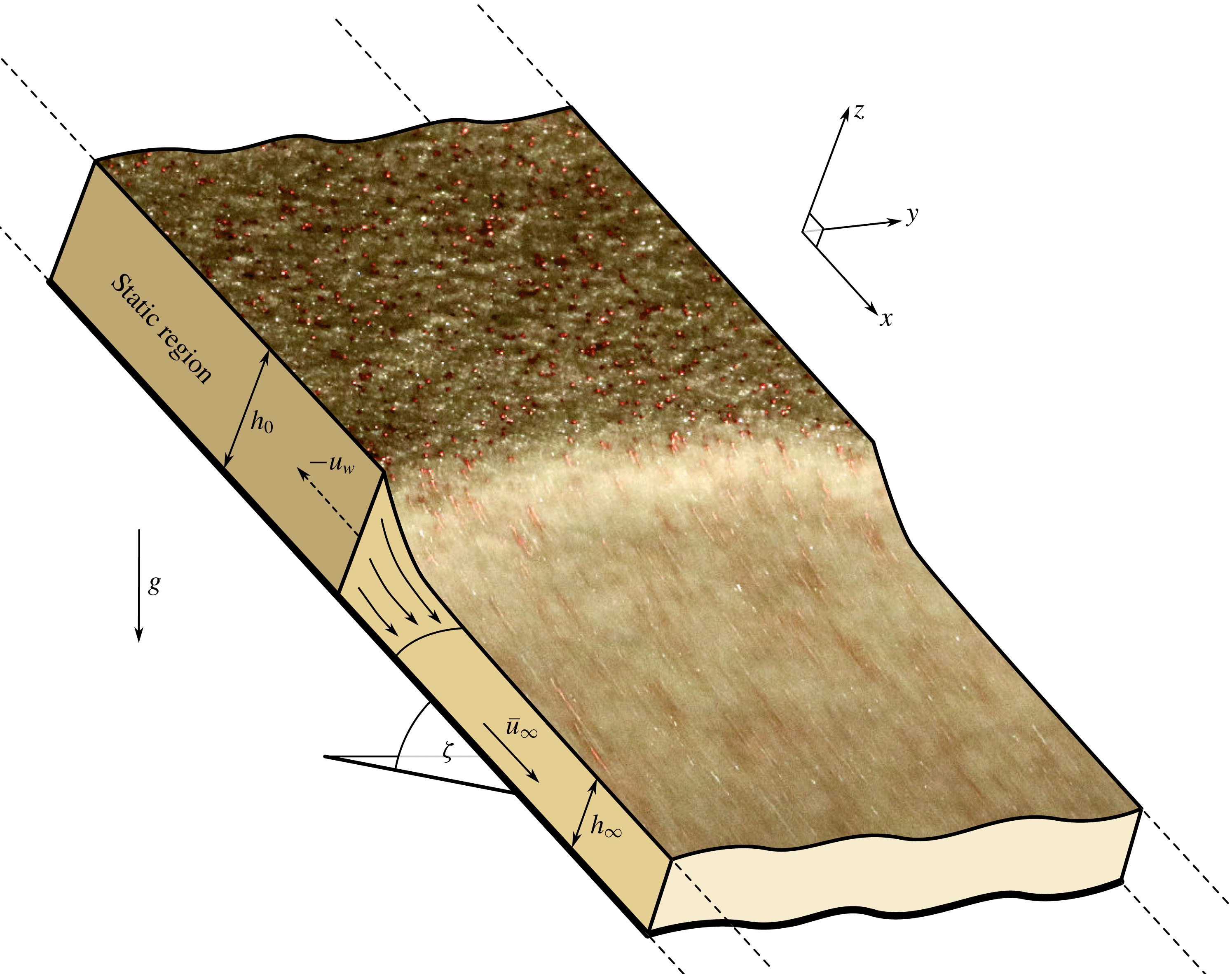
Retrogressive failures are also observed in small-scale dry granular flow experiments (e.g. Daerr & Douady Reference Daerr and Douady1999; Daerr Reference Daerr2001, and those performed in this paper). Figure 1 shows an example of an approximately planar retrogressive wavefront, generated by a straight perturbation across the full width of the inclined plane (figure 2). The retrogressive wave separates a thicker upslope layer of static grains from a thinner downstream layer of flowing grains. In the experiments of Daerr & Douady (Reference Daerr and Douady1999) and Daerr (Reference Daerr2001) the failure was initiated at a single point and so generated a non-planar retrogressive failure, instead. In their experiments a static layer of thickness
 $h_{stop}(\unicode[STIX]{x1D701})$
was created by pouring 180–
$h_{stop}(\unicode[STIX]{x1D701})$
was created by pouring 180–
 $300~\unicode[STIX]{x03BC}\text{m}$
diameter glass beads down a plane covered with velvet cloth and inclined at an angle
$300~\unicode[STIX]{x03BC}\text{m}$
diameter glass beads down a plane covered with velvet cloth and inclined at an angle
 $\unicode[STIX]{x1D701}$
to the horizontal. Due to frictional hysteresis, the layer remained static until the inclination angle was increased, up to an angle
$\unicode[STIX]{x1D701}$
to the horizontal. Due to frictional hysteresis, the layer remained static until the inclination angle was increased, up to an angle
 $\unicode[STIX]{x1D701}_{start}(h)>\unicode[STIX]{x1D701}$
, at which the layer spontaneously started flowing. Inclining the static layer to an angle only slightly larger than
$\unicode[STIX]{x1D701}_{start}(h)>\unicode[STIX]{x1D701}$
, at which the layer spontaneously started flowing. Inclining the static layer to an angle only slightly larger than
 $\unicode[STIX]{x1D701}$
and then perturbing it, resulted in an avalanche that propagated only downhill from the point of disturbance, whereas perturbing a layer that had been inclined further caused an additional upward retrogressive failure, propagating at a constant speed. Daerr (Reference Daerr2001) showed that, at a certain inclination angle, the behaviour immediately switched from a downslope avalanche to a retrogressive failure in which the wave propagated upslope at a non-zero speed, i.e. there is a finite wave speed at the onset of retrogressive failure. The same qualitative behaviour also occurs in the retrogressive failures studied in this paper, but the fact that they are planar makes them more amenable to analysis.
$\unicode[STIX]{x1D701}$
and then perturbing it, resulted in an avalanche that propagated only downhill from the point of disturbance, whereas perturbing a layer that had been inclined further caused an additional upward retrogressive failure, propagating at a constant speed. Daerr (Reference Daerr2001) showed that, at a certain inclination angle, the behaviour immediately switched from a downslope avalanche to a retrogressive failure in which the wave propagated upslope at a non-zero speed, i.e. there is a finite wave speed at the onset of retrogressive failure. The same qualitative behaviour also occurs in the retrogressive failures studied in this paper, but the fact that they are planar makes them more amenable to analysis.
The experimental set-up consisting of a rough plane, inclined at an angle
 $\unicode[STIX]{x1D701}$
to the horizontal, which has a monolayer of spherical glass beads of diameter 750–
$\unicode[STIX]{x1D701}$
to the horizontal, which has a monolayer of spherical glass beads of diameter 750–
 $1000~\unicode[STIX]{x03BC}\text{m}$
stuck to the surface, to create no slip at the base. A hopper and a gate at the top of the chute are used to create a deposit of thickness
$1000~\unicode[STIX]{x03BC}\text{m}$
stuck to the surface, to create no slip at the base. A hopper and a gate at the top of the chute are used to create a deposit of thickness
 $h_{stop}$
by generating a steady uniform flow and then closing the mass supply. The laser profilometer (Micro-Epsilon scanCONTROL 2700-100) is mounted normal to the inclined plane in order to measure the flow thickness. A set of coordinates
$h_{stop}$
by generating a steady uniform flow and then closing the mass supply. The laser profilometer (Micro-Epsilon scanCONTROL 2700-100) is mounted normal to the inclined plane in order to measure the flow thickness. A set of coordinates
 $Oxyz$
is defined with the
$Oxyz$
is defined with the
 $x$
-axis pointing downslope, the
$x$
-axis pointing downslope, the
 $y$
-axis across the slope and the
$y$
-axis across the slope and the
 $z$
-axis along the upward pointing normal. A typical retrogressive wave experiment is shown in movie 3 in the online supplementary material.
$z$
-axis along the upward pointing normal. A typical retrogressive wave experiment is shown in movie 3 in the online supplementary material.
Daerr & Douady (Reference Daerr and Douady1999) and Daerr (Reference Daerr2001) termed the retrogressive failures ‘uphill-propagating avalanches’. These were investigated theoretically by Bouchaud & Cates (Reference Bouchaud and Cates1998) using the Bouchaud, Cates, Ravi Prakash and Edwards (BCRE) model (Bouchaud et al. Reference Bouchaud, Cates, Prakesh and Edwards1994) in which a granular material is separated into two phases; rolling and static. Although this was a purely kinematic model, it was able to capture the transition between non-retrogressive and retrogressive failure. However, with the BCRE model this transition occurred smoothly, i.e. there was a smooth variation of the retrogressive wave speed starting from zero when the wave does not move upslope, which contradicts the experimental results of Daerr (Reference Daerr2001). Aranson & Tsimring (Reference Aranson and Tsimring2001, Reference Aranson and Tsimring2002) captured the retrogressive failures using a partially fluidised granular flow model with an order parameter equation to represent the transition between static and flowing grains. Using this model they found that the uphill-propagating front was a travelling wave solution with the onset occurring through a discontinuity in the speed of the retrogressive waves, i.e. the wave speed immediately jumped up from zero (for no upslope propagation) to a finite non-zero value. Their theoretical prediction for the existence of uphill waves agreed with the experimental data of Daerr & Douady (Reference Daerr and Douady1999) and Daerr (Reference Daerr2001), using one fitting parameter. These models of retrogressive failure (Aranson & Tsimring Reference Aranson and Tsimring2001, Reference Aranson and Tsimring2002) are, however, phenomenological in nature (Aradian, Raphaël & De Gennes Reference Aradian, Raphaël and De Gennes2002), since the grain inertia is neglected and there is some uncertainty in the physics underlying the order parameter and its governing equation.
In this paper, it is shown that the retrogressive wave speed, as well as the jump in the wave speed at the non-retrogressive/retrogressive failure transition, can be quantitatively predicted by using a depth-averaged avalanche model with a non-monotonic effective basal friction law (Pouliquen & Forterre Reference Pouliquen and Forterre2002; Edwards et al.
Reference Edwards, Viroulet, Kokelaar and Gray2017, Reference Edwards, Russell, Johnson and Gray2019). The non-monotonic friction law encodes the hysteresis that leads to
 $h_{stop}(\unicode[STIX]{x1D701})$
and
$h_{stop}(\unicode[STIX]{x1D701})$
and
 $h_{start}(\unicode[STIX]{x1D701})$
(the inverse function of
$h_{start}(\unicode[STIX]{x1D701})$
(the inverse function of
 $\unicode[STIX]{x1D701}_{start}(h)$
) and consists of (i) a dynamic regime, which is a monotonically increasing function of the speed at moderate to high Froude numbers (Pouliquen Reference Pouliquen1999a
), (ii) a multi-valued static friction when the Froude number is zero and (iii) a monotonically decreasing regime that interpolates between the maximum static friction and the minimum dynamic friction at low Froude numbers (Pouliquen & Forterre Reference Pouliquen and Forterre2002). In addition, Edwards et al. (Reference Edwards, Viroulet, Kokelaar and Gray2017, Reference Edwards, Russell, Johnson and Gray2019) showed that there was another important thickness
$\unicode[STIX]{x1D701}_{start}(h)$
) and consists of (i) a dynamic regime, which is a monotonically increasing function of the speed at moderate to high Froude numbers (Pouliquen Reference Pouliquen1999a
), (ii) a multi-valued static friction when the Froude number is zero and (iii) a monotonically decreasing regime that interpolates between the maximum static friction and the minimum dynamic friction at low Froude numbers (Pouliquen & Forterre Reference Pouliquen and Forterre2002). In addition, Edwards et al. (Reference Edwards, Viroulet, Kokelaar and Gray2017, Reference Edwards, Russell, Johnson and Gray2019) showed that there was another important thickness
 $h_{\ast }\in (h_{stop},h_{start})$
, which defines the transition between intermediate and dynamic regimes and is the minimum observable steady uniform flow thickness.
$h_{\ast }\in (h_{stop},h_{start})$
, which defines the transition between intermediate and dynamic regimes and is the minimum observable steady uniform flow thickness.
Depth-integrated avalanche theories of this sort are widely used for modelling shallow granular free-surface flows and are closely related to the shallow water, or St Venant equations, of fluid mechanics. The first derivation for granular flows was by Savage & Hutter (Reference Savage and Hutter1989, Reference Savage and Hutter1991) assuming an incompressible flow with a Mohr–Coulomb rheology and a constant Coulomb basal friction coefficient. This yielded a shallow-water-like system of conservation laws with additional source terms due to gravity, basal friction and topography gradients, as well as an ‘earth pressure’ coefficient multiplying the depth-integrated pressure, which took active and passive values dependent on whether the flows were dilatational or compressional. In this paper, as in many recent works, the earth pressure coefficient is assumed to be unity (Gray, Wieland & Hutter Reference Gray, Wieland and Hutter1999; Pouliquen Reference Pouliquen1999b ; Gray, Tai & Noelle Reference Gray, Tai and Noelle2003). The model has been generalised to two-dimensional flows over complex topography (Gray et al. Reference Gray, Wieland and Hutter1999; Wieland, Gray & Hutter Reference Wieland, Gray and Hutter1999; Mangeney-Castelnau et al. Reference Mangeney-Castelnau, Vilotte, Bristeau, Perthame, Bouchut, Simeoni and Yerneni2003; Pudasaini & Hutter Reference Pudasaini and Hutter2003; Bouchut & Westdickenberg Reference Bouchut and Westdickenberg2004; Luca et al. Reference Luca, Hutter, Tai and Kuo2009) and has been widely used in the snow avalanche community for hazard zone mapping (Grigorian, Eglit & Iakimov Reference Grigorian, Eglit and Iakimov1967; Naaim et al. Reference Naaim, Naaim-Bouvet, Faug and Bouchet2004; Sampl & Zwinger Reference Sampl and Zwinger2004; Christen, Kowalski & Bartelt Reference Christen, Kowalski and Bartelt2010; Fischer, Kowalski & Pudasaini Reference Fischer, Kowalski and Pudasaini2012). Analogous theories have been developed for debris flows (Iverson Reference Iverson1997; Iverson & Denlinger Reference Iverson and Denlinger2001; Denlinger & Iverson Reference Denlinger and Iverson2001; Johnson et al. Reference Johnson, Kokelaar, Iverson, Logan, LaHusen and Gray2012), pyroclastic flows (Pitman et al. Reference Pitman, Nichita, Patra, Bauer, Sheridan and Bursik2003; Mangeney et al. Reference Mangeney, Bouchut, Thomas, Vilotte and Bristeau2007; Doyle, Hogg & Mader Reference Doyle, Hogg and Mader2011) and landslides (Kuo et al. Reference Kuo, Tai, Bouchut, Mangeney, Pelanti, Chen and Chang2009; Mangeney et al. Reference Mangeney, Roche, Hungr, Mangold, Faccanoni and Lucas2010).
The constant Coulomb basal friction of Savage & Hutter (Reference Savage and Hutter1989) provides a good description of dry granular flows over smooth surfaces. However, the basal friction felt by flows over a rough surface, i.e. where the bed roughness approaches or exceeds the mean particle diameter, is strongly dependent on both the flow thickness and the speed (Pouliquen & Forterre Reference Pouliquen and Forterre2002). Gray & Edwards (Reference Gray and Edwards2014) showed that by formally depth averaging the
 $\unicode[STIX]{x1D707}(I)$
-rheology for granular flows (GDR-MiDi 2004; Jop, Forterre & Pouliquen Reference Jop, Forterre and Pouliquen2006) and exploiting the shallowness of the system, the shallow-water-like avalanche equations emerge naturally, at leading order in the aspect ratio, with an effective basal friction corresponding to Pouliquen & Forterre’s (Reference Pouliquen and Forterre2002) dynamic regime described above. However, since frictional hysteresis is key to the formation of retrogressive failures, it is necessary to augment the model with the intermediate and static regimes, at low and zero Froude numbers respectively (Pouliquen & Forterre Reference Pouliquen and Forterre2002; Edwards et al.
Reference Edwards, Viroulet, Kokelaar and Gray2017, Reference Edwards, Russell, Johnson and Gray2019).
$\unicode[STIX]{x1D707}(I)$
-rheology for granular flows (GDR-MiDi 2004; Jop, Forterre & Pouliquen Reference Jop, Forterre and Pouliquen2006) and exploiting the shallowness of the system, the shallow-water-like avalanche equations emerge naturally, at leading order in the aspect ratio, with an effective basal friction corresponding to Pouliquen & Forterre’s (Reference Pouliquen and Forterre2002) dynamic regime described above. However, since frictional hysteresis is key to the formation of retrogressive failures, it is necessary to augment the model with the intermediate and static regimes, at low and zero Froude numbers respectively (Pouliquen & Forterre Reference Pouliquen and Forterre2002; Edwards et al.
Reference Edwards, Viroulet, Kokelaar and Gray2017, Reference Edwards, Russell, Johnson and Gray2019).
The retrogressive failures are particularly sensitive to the intermediate (velocity-decreasing) part of the friction law, which, in the absence of direct experimental observations, has previously been described by a power-law interpolation between the maximum static and minimum dynamic friction (Pouliquen & Forterre Reference Pouliquen and Forterre2002). Retrogressive failures are therefore not just of fundamental scientific interest, but also provide an important test case for the friction law proposed by Edwards et al. (Reference Edwards, Viroulet, Kokelaar and Gray2017, Reference Edwards, Russell, Johnson and Gray2019).
2 Experimental observations
The experimental set-up consists of a plane (1.65 m long by 0.58 m wide) that is inclined at an angle
 $\unicode[STIX]{x1D701}$
to the horizontal as shown in figure 2. The plane is roughened with a monolayer of spherical glass beads of diameter 750–
$\unicode[STIX]{x1D701}$
to the horizontal as shown in figure 2. The plane is roughened with a monolayer of spherical glass beads of diameter 750–
 $1000~\unicode[STIX]{x03BC}\text{m}$
(to ensure no basal slip, Silbert et al.
Reference Silbert, Ertas, Grest, Halsey, Levine and Plimpton2001; Goujon, Thomas & Dalloz-Dubrujeaud Reference Goujon, Thomas and Dalloz-Dubrujeaud2003; Jing et al.
Reference Jing, Kwok, Leung and Sobral2016), which are attached using double-sided sticky tape. To start an experiment, the plane is inclined to an angle
$1000~\unicode[STIX]{x03BC}\text{m}$
(to ensure no basal slip, Silbert et al.
Reference Silbert, Ertas, Grest, Halsey, Levine and Plimpton2001; Goujon, Thomas & Dalloz-Dubrujeaud Reference Goujon, Thomas and Dalloz-Dubrujeaud2003; Jing et al.
Reference Jing, Kwok, Leung and Sobral2016), which are attached using double-sided sticky tape. To start an experiment, the plane is inclined to an angle
 $\unicode[STIX]{x1D701}_{0}$
and glass beads, of diameter 125–
$\unicode[STIX]{x1D701}_{0}$
and glass beads, of diameter 125–
 $160~\unicode[STIX]{x03BC}\text{m}$
, are released from a hopper at the top of the chute to form a steady uniform flow. As this flow ceases, it forms a static layer of uniform thickness
$160~\unicode[STIX]{x03BC}\text{m}$
, are released from a hopper at the top of the chute to form a steady uniform flow. As this flow ceases, it forms a static layer of uniform thickness
 $h_{0}=h_{stop}(\unicode[STIX]{x1D701}_{0})$
at its trailing edge (Edwards et al.
Reference Edwards, Russell, Johnson and Gray2019). The inclination of the chute is then carefully increased to an angle
$h_{0}=h_{stop}(\unicode[STIX]{x1D701}_{0})$
at its trailing edge (Edwards et al.
Reference Edwards, Russell, Johnson and Gray2019). The inclination of the chute is then carefully increased to an angle
 $\unicode[STIX]{x1D701}>\unicode[STIX]{x1D701}_{0}$
. Provided that the new inclination angle is not too large, i.e.
$\unicode[STIX]{x1D701}>\unicode[STIX]{x1D701}_{0}$
. Provided that the new inclination angle is not too large, i.e.
 $\unicode[STIX]{x1D701}<\unicode[STIX]{x1D701}_{start}(h_{0})$
, frictional hysteresis keeps the grains static. The resulting layer is described as being metastable (Daerr Reference Daerr2001) because it can exist in either a flowing or static state, where the static state is stable to infinitesimal perturbations, but unstable to sufficiently large finite perturbations.
$\unicode[STIX]{x1D701}<\unicode[STIX]{x1D701}_{start}(h_{0})$
, frictional hysteresis keeps the grains static. The resulting layer is described as being metastable (Daerr Reference Daerr2001) because it can exist in either a flowing or static state, where the static state is stable to infinitesimal perturbations, but unstable to sufficiently large finite perturbations.
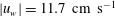
Overhead photographs showing a time sequence of the retrogressive failure front. It spans the width of each image and separates the initially stationary layer of 125–
 $160~\unicode[STIX]{x03BC}\text{m}$
glass beads (in focus at the top of each picture) from the flowing material below (blurred by the exposure time of
$160~\unicode[STIX]{x03BC}\text{m}$
glass beads (in focus at the top of each picture) from the flowing material below (blurred by the exposure time of
 $1/50$
s). The retrogressive front propagates upslope with speed
$1/50$
s). The retrogressive front propagates upslope with speed
 $|u_{w}|=11.7~\text{cm}~\text{s}^{-1}$
, and continues to do so until it reaches the top of the static layer. The time-dependent evolution of the wave can be seen in movie 4 in the online supplementary material.
$|u_{w}|=11.7~\text{cm}~\text{s}^{-1}$
, and continues to do so until it reaches the top of the static layer. The time-dependent evolution of the wave can be seen in movie 4 in the online supplementary material.
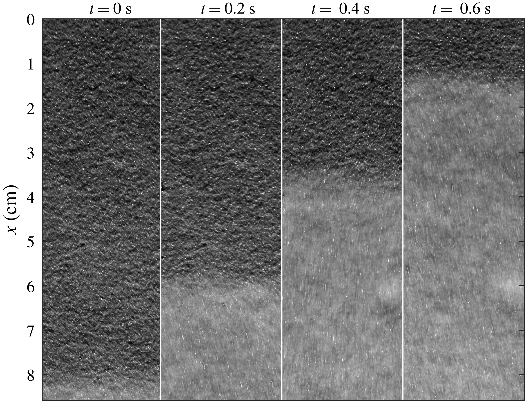
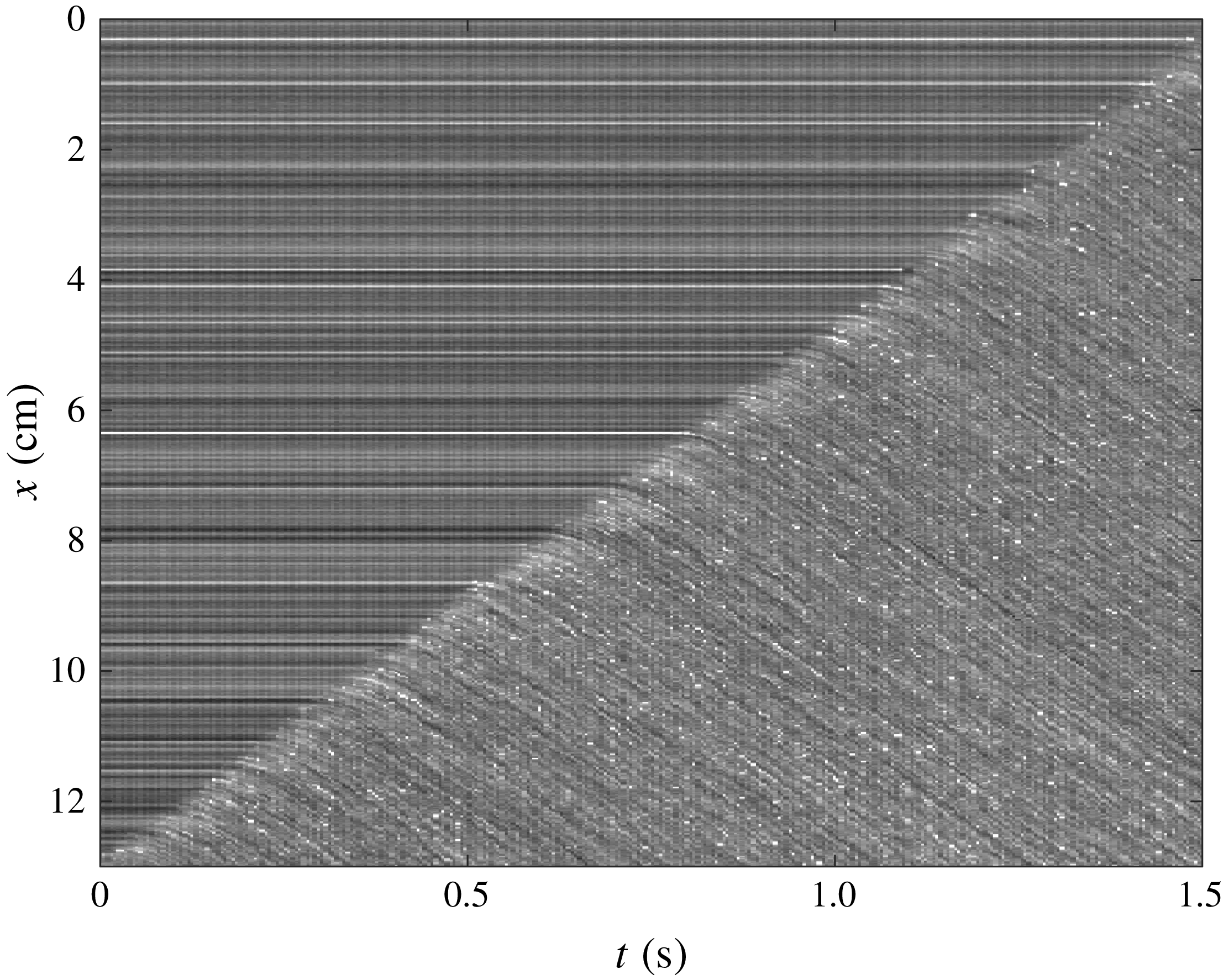
The layer is destabilised by tapping it near the bottom with a ruler held horizontally across the chute. After a rapid initial transient, the retrogressive failure propagates upwards at a constant speed, and remains approximately straight and perpendicular to the downslope direction as shown in figure 3 and supplementary movies 1–4. The grains that have been eroded by this retrogressive failure form a steady uniform flow of thickness
 $h_{\infty }<h_{0}$
downstream of the wavefront. The propagation speed of the retrogressive front is determined by a high-speed camera (Teledyne DALSA Genie HM1400), which takes overhead photographs at 200 frames per second. Figure 4 shows a typical space–time plot that is constructed by extracting the middle row of pixels down the centre of the chute from each image and combining them into a single plot with time
$h_{\infty }<h_{0}$
downstream of the wavefront. The propagation speed of the retrogressive front is determined by a high-speed camera (Teledyne DALSA Genie HM1400), which takes overhead photographs at 200 frames per second. Figure 4 shows a typical space–time plot that is constructed by extracting the middle row of pixels down the centre of the chute from each image and combining them into a single plot with time
 $t$
on the abscissa and downstream distance
$t$
on the abscissa and downstream distance
 $x$
on the ordinate. Oblique illumination from the bottom of the chute makes the retrogressive front clearly visible as a diagonal line. The gradient of this line is measured to obtain the front propagation speed
$x$
on the ordinate. Oblique illumination from the bottom of the chute makes the retrogressive front clearly visible as a diagonal line. The gradient of this line is measured to obtain the front propagation speed
 $|u_{w}|$
.
$|u_{w}|$
.
A space–time plot for
 $\unicode[STIX]{x1D701}_{0}=24^{\circ }$
,
$\unicode[STIX]{x1D701}_{0}=24^{\circ }$
,
 $\unicode[STIX]{x1D701}=27.5^{\circ }$
and
$\unicode[STIX]{x1D701}=27.5^{\circ }$
and
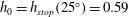
 $h_{0}=h_{stop}(24^{\circ })=0.95$
mm. The horizontal straight lines indicate material that is static and the more speckled region indicates flowing material. The interface between these two regions is the retrogressive failure front, which propagates upslope at speed
$h_{0}=h_{stop}(24^{\circ })=0.95$
mm. The horizontal straight lines indicate material that is static and the more speckled region indicates flowing material. The interface between these two regions is the retrogressive failure front, which propagates upslope at speed
 $|u_{w}|=8.5~\text{cm}~\text{s}^{-1}$
. The steady uniform flow downslope of the front causes faint diagonal lines whose gradient implies that the surface velocity rapidly accelerates to
$|u_{w}|=8.5~\text{cm}~\text{s}^{-1}$
. The steady uniform flow downslope of the front causes faint diagonal lines whose gradient implies that the surface velocity rapidly accelerates to
 $u_{s}=8.1~\text{cm}~\text{s}^{-1}$
.
$u_{s}=8.1~\text{cm}~\text{s}^{-1}$
.
Measurements of the flow thickness
 $h$
during the retrogressive failure with an initial layer thickness
$h$
during the retrogressive failure with an initial layer thickness
 $h_{0}=h_{stop}(25^{\circ })=0.59$
mm and current inclination angle
$h_{0}=h_{stop}(25^{\circ })=0.59$
mm and current inclination angle
 $\unicode[STIX]{x1D701}=27.5^{\circ }$
. (a) An instantaneous snapshot of the thickness profile as a function of downslope distance
$\unicode[STIX]{x1D701}=27.5^{\circ }$
. (a) An instantaneous snapshot of the thickness profile as a function of downslope distance
 $x-x_{0}$
, where the constant
$x-x_{0}$
, where the constant
 $x_{0}$
is the position of the failure. The measured noise is of the order of one grain diameter. (b) Average of 1160 such profiles acquired at 1 ms intervals and plotted with respect to a coordinate
$x_{0}$
is the position of the failure. The measured noise is of the order of one grain diameter. (b) Average of 1160 such profiles acquired at 1 ms intervals and plotted with respect to a coordinate
 $\unicode[STIX]{x1D709}=x-u_{w}t$
, which moves upstream at constant speed
$\unicode[STIX]{x1D709}=x-u_{w}t$
, which moves upstream at constant speed
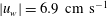 $|u_{w}|=6.9~\text{cm}~\text{s}^{-1}$
.
$|u_{w}|=6.9~\text{cm}~\text{s}^{-1}$
.
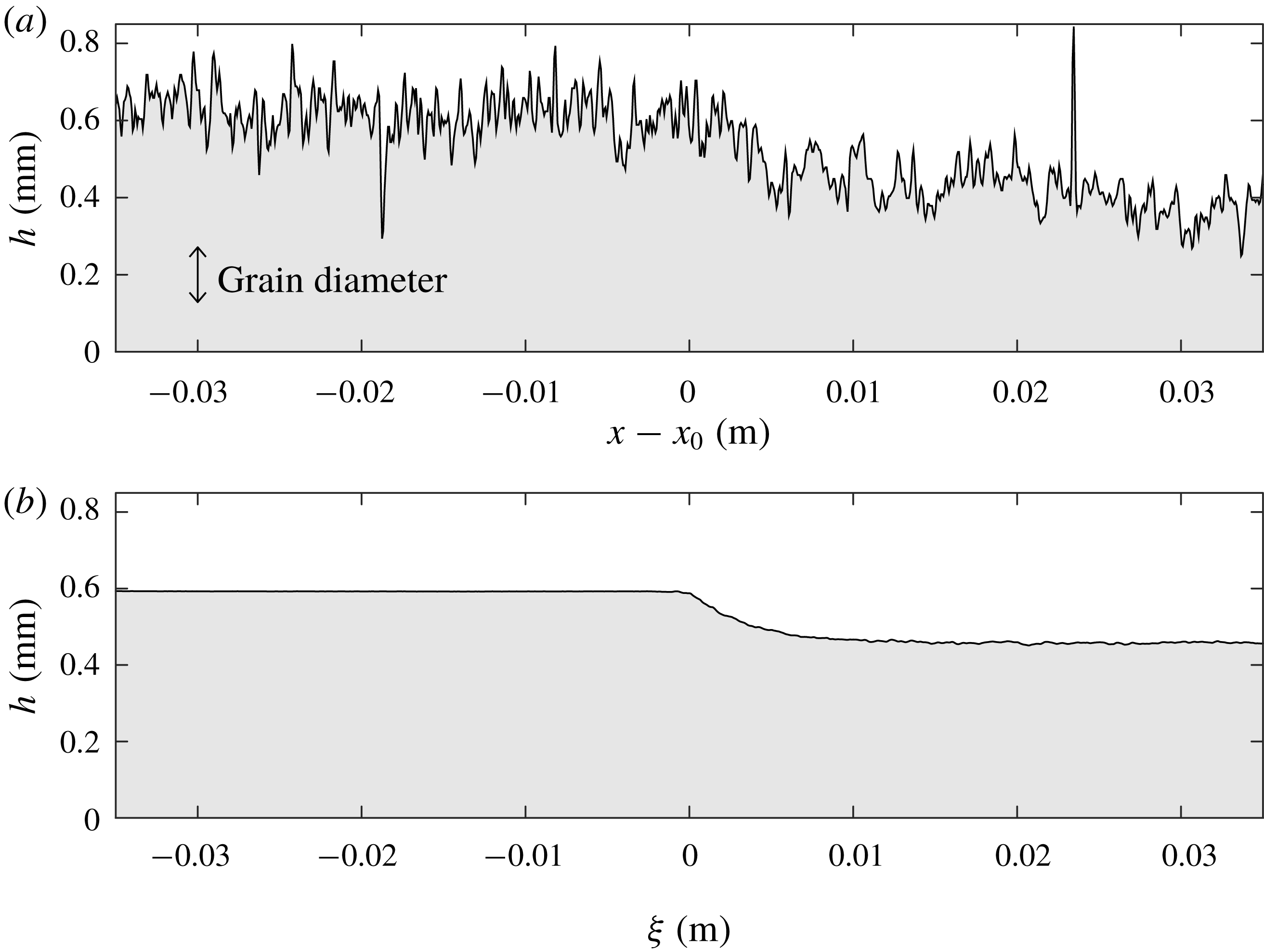
Measurements of the flow thickness using a laser profilometer (Micro-Epsilon scanCONTROL 2700-100) are used to quantify the decrease in flow thickness
 $h$
that occurs across the retrogressive failure. For a typical experimental flow, illustrated in figure 5(a), this decrease is
$h$
that occurs across the retrogressive failure. For a typical experimental flow, illustrated in figure 5(a), this decrease is
 ${\sim}0.13$
mm, which is approximately one grain diameter and is similar to the measured roughness of the free-surface profile. An average of many such thickness profiles in a frame moving upslope with the wave, at speed
${\sim}0.13$
mm, which is approximately one grain diameter and is similar to the measured roughness of the free-surface profile. An average of many such thickness profiles in a frame moving upslope with the wave, at speed
 $|u_{w}|$
, and plotted with respect to the frame coordinate
$|u_{w}|$
, and plotted with respect to the frame coordinate
 $\unicode[STIX]{x1D709}=x-u_{w}t$
(figure 5
b) provides a clearer picture of the shape of the retrogressive wave. Upslope of the wave (
$\unicode[STIX]{x1D709}=x-u_{w}t$
(figure 5
b) provides a clearer picture of the shape of the retrogressive wave. Upslope of the wave (
 $\unicode[STIX]{x1D709}<0$
) the grains form a uniform thickness static layer. At the point of failure
$\unicode[STIX]{x1D709}<0$
) the grains form a uniform thickness static layer. At the point of failure
 $\unicode[STIX]{x1D709}=0$
the surface gradient
$\unicode[STIX]{x1D709}=0$
the surface gradient
 $\unicode[STIX]{x2202}h/\unicode[STIX]{x2202}\unicode[STIX]{x1D709}$
rapidly steepens and the flow transitions smoothly to a thinner, uniform flowing layer downslope of the failure. The averaged experimental data in figure 5(b) indicate that this transition occurs over a length scale of 6–7 mm, although instantaneous measurements (figure 5
a) suggest that the wave may be slightly narrower (
$\unicode[STIX]{x2202}h/\unicode[STIX]{x2202}\unicode[STIX]{x1D709}$
rapidly steepens and the flow transitions smoothly to a thinner, uniform flowing layer downslope of the failure. The averaged experimental data in figure 5(b) indicate that this transition occurs over a length scale of 6–7 mm, although instantaneous measurements (figure 5
a) suggest that the wave may be slightly narrower (
 ${<}5$
mm). The exact retrogressive failure solutions that will be constructed in § 5 have a thickness profile that is almost identical to the dataset shown in figure 5(b).
${<}5$
mm). The exact retrogressive failure solutions that will be constructed in § 5 have a thickness profile that is almost identical to the dataset shown in figure 5(b).
3 Governing equations
3.1 Depth-averaged avalanche model
The retrogressive wave has a shallow aspect ratio (figure 5
b) and is nearly uniform in the cross-slope direction (figure 3), which motivates the use of a one-dimensional depth-integrated avalanche model to describe the flow. The flow thickness
 $h(x,t)$
and depth-averaged downslope velocity
$h(x,t)$
and depth-averaged downslope velocity
 $\bar{u}(x,t)$
therefore satisfy the depth-integrated mass and momentum equations
$\bar{u}(x,t)$
therefore satisfy the depth-integrated mass and momentum equations
 $$\begin{eqnarray}\displaystyle & \displaystyle \frac{\unicode[STIX]{x2202}h}{\unicode[STIX]{x2202}t}+\frac{\unicode[STIX]{x2202}}{\unicode[STIX]{x2202}x}(h\bar{u})=0, & \displaystyle\end{eqnarray}$$
 $$\begin{eqnarray}\displaystyle & \displaystyle \frac{\unicode[STIX]{x2202}}{\unicode[STIX]{x2202}t}(h\bar{u})+\frac{\unicode[STIX]{x2202}}{\unicode[STIX]{x2202}x}(\unicode[STIX]{x1D712}h\bar{u}^{2})+\frac{\unicode[STIX]{x2202}}{\unicode[STIX]{x2202}x}\left(\frac{1}{2}gh^{2}\cos \unicode[STIX]{x1D701}\right)=ghS\cos \unicode[STIX]{x1D701}, & \displaystyle\end{eqnarray}$$
where
 $x$
is the downslope coordinate,
$x$
is the downslope coordinate,
 $t$
is time,
$t$
is time,
 $\unicode[STIX]{x1D712}=\overline{u^{2}}/\bar{u}^{2}$
is the shape factor,
$\unicode[STIX]{x1D712}=\overline{u^{2}}/\bar{u}^{2}$
is the shape factor,
 $\unicode[STIX]{x1D701}$
is the chute inclination angle,
$\unicode[STIX]{x1D701}$
is the chute inclination angle,
 $S$
is the non-dimensional net acceleration and
$S$
is the non-dimensional net acceleration and
 $g$
is the constant of gravitational acceleration. For deep flows on rough beds, a steady uniform flow will develop into a Bagnold velocity profile (GDR-MiDi 2004; Gray & Edwards Reference Gray and Edwards2014) and the shape factor
$g$
is the constant of gravitational acceleration. For deep flows on rough beds, a steady uniform flow will develop into a Bagnold velocity profile (GDR-MiDi 2004; Gray & Edwards Reference Gray and Edwards2014) and the shape factor
 $\unicode[STIX]{x1D712}=5/4$
, while for thinner flows close to
$\unicode[STIX]{x1D712}=5/4$
, while for thinner flows close to
 $h_{stop}$
weakly exponential profiles develop (Kamrin & Henann Reference Kamrin and Henann2015), which have a shape factor of approximately 1.53 for the typical profiles observed in our experiments. Solutions to this system are, however, quite insensitive to the value of the shape factor due to the low value of Froude number (Saingier, Deboeuf & Lagrée Reference Saingier, Deboeuf and Lagrée2016; Viroulet et al.
Reference Viroulet, Baker, Edwards, Johnson, Gjaltema, Clavel and Gray2017). Therefore it is assumed here that
$h_{stop}$
weakly exponential profiles develop (Kamrin & Henann Reference Kamrin and Henann2015), which have a shape factor of approximately 1.53 for the typical profiles observed in our experiments. Solutions to this system are, however, quite insensitive to the value of the shape factor due to the low value of Froude number (Saingier, Deboeuf & Lagrée Reference Saingier, Deboeuf and Lagrée2016; Viroulet et al.
Reference Viroulet, Baker, Edwards, Johnson, Gjaltema, Clavel and Gray2017). Therefore it is assumed here that
 $\unicode[STIX]{x1D712}=1$
, because it significantly simplifies the characteristic structure of the equations (see e.g. Savage & Hutter Reference Savage and Hutter1989; Gray et al.
Reference Gray, Wieland and Hutter1999; Pouliquen Reference Pouliquen1999b
; Gray et al.
Reference Gray, Tai and Noelle2003; Pouliquen & Forterre Reference Pouliquen and Forterre2002; Gray & Edwards Reference Gray and Edwards2014). The characteristic speeds of the hyperbolic system (3.1)–(3.2) are then
$\unicode[STIX]{x1D712}=1$
, because it significantly simplifies the characteristic structure of the equations (see e.g. Savage & Hutter Reference Savage and Hutter1989; Gray et al.
Reference Gray, Wieland and Hutter1999; Pouliquen Reference Pouliquen1999b
; Gray et al.
Reference Gray, Tai and Noelle2003; Pouliquen & Forterre Reference Pouliquen and Forterre2002; Gray & Edwards Reference Gray and Edwards2014). The characteristic speeds of the hyperbolic system (3.1)–(3.2) are then
 $$\begin{eqnarray}\displaystyle c_{\pm }=\bar{u}\pm \sqrt{gh\cos \unicode[STIX]{x1D701}}, & & \displaystyle\end{eqnarray}$$
and the ratio of flow speed to the gravity wave speed defines the Froude number
 $$\begin{eqnarray}\displaystyle Fr=\frac{|\bar{u}|}{\sqrt{gh\cos \unicode[STIX]{x1D701}}}. & & \displaystyle\end{eqnarray}$$
The non-dimensional net acceleration
 $S$
in the source term on the right-hand side of (3.2) is defined as the difference between the downslope component of gravity and the effective basal friction
$S$
in the source term on the right-hand side of (3.2) is defined as the difference between the downslope component of gravity and the effective basal friction
 $\unicode[STIX]{x1D707}(h,Fr)$
 $$\begin{eqnarray}\displaystyle S=\tan \unicode[STIX]{x1D701}-\unicode[STIX]{x1D707}(h,Fr)(\bar{u}/|\bar{u}|), & & \displaystyle\end{eqnarray}$$
where the factor
 $\bar{u}/|\bar{u}|$
ensures that the basal friction always opposes the direction of motion. In this paper the friction always acts upslope irrespective of whether the material is moving or static and hence
$\bar{u}/|\bar{u}|$
ensures that the basal friction always opposes the direction of motion. In this paper the friction always acts upslope irrespective of whether the material is moving or static and hence
 $\bar{u}/|\bar{u}|=1$
. The non-dimensional net acceleration
$\bar{u}/|\bar{u}|=1$
. The non-dimensional net acceleration
 $S$
determines whether a constant thickness layer will accelerate (
$S$
determines whether a constant thickness layer will accelerate (
 $S>0$
), decelerate (
$S>0$
), decelerate (
 $S<0$
) or move with constant speed (
$S<0$
) or move with constant speed (
 $S=0$
).
$S=0$
).
It is important to note that the depth-averaged viscous terms (Gray & Edwards Reference Gray and Edwards2014; Baker, Barker & Gray Reference Baker, Barker and Gray2016a ), which are crucial for the formation of leveed channels on non-erodible slopes (Rocha, Johnson & Gray Reference Rocha, Johnson and Gray2019), can be neglected here because the retrogressive failures are planar. It is, however, anticipated that viscous terms could well be important for non-planar retrogressive waves, where cross-slope gradients in the velocity will develop naturally, or, for the correct cutoff frequency and coarsening dynamics of roll waves and erosion–deposition waves that may form downstream of the failure front (Gray & Edwards Reference Gray and Edwards2014; Edwards & Gray Reference Edwards and Gray2015; Viroulet et al. Reference Viroulet, Baker, Rocha, Johnson, Kokelaar and Gray2018).
3.2 The non-monotonic effective basal friction law
Gray & Edwards (Reference Gray and Edwards2014) showed that, to leading order in the aspect ratio, both the inviscid avalanche equations (3.1)–(3.2) and the dynamic friction law of Pouliquen & Forterre (Reference Pouliquen and Forterre2002) emerge naturally from depth averaging the
 $\unicode[STIX]{x1D707}(I)$
-rheology for granular flows (GDR-MiDi 2004; Jop et al.
Reference Jop, Forterre and Pouliquen2006). In order to model coexisting regions of static and flowing material it is necessary to augment the dynamic regime (
$\unicode[STIX]{x1D707}(I)$
-rheology for granular flows (GDR-MiDi 2004; Jop et al.
Reference Jop, Forterre and Pouliquen2006). In order to model coexisting regions of static and flowing material it is necessary to augment the dynamic regime (
 $Fr\geqslant \unicode[STIX]{x1D6FD}_{\ast }$
) with the multi-valued static (
$Fr\geqslant \unicode[STIX]{x1D6FD}_{\ast }$
) with the multi-valued static (
 $Fr=0$
) and intermediate (
$Fr=0$
) and intermediate (
 $0<Fr<\unicode[STIX]{x1D6FD}_{\ast }$
) regimes (Pouliquen & Forterre Reference Pouliquen and Forterre2002; Edwards et al.
Reference Edwards, Viroulet, Kokelaar and Gray2017, Reference Edwards, Russell, Johnson and Gray2019). For glass ballotini (which does not have an offset
$0<Fr<\unicode[STIX]{x1D6FD}_{\ast }$
) regimes (Pouliquen & Forterre Reference Pouliquen and Forterre2002; Edwards et al.
Reference Edwards, Viroulet, Kokelaar and Gray2017, Reference Edwards, Russell, Johnson and Gray2019). For glass ballotini (which does not have an offset
 $\unicode[STIX]{x1D6E4}$
in the empirical flow rule) the non-monotonic friction law of Edwards et al. (Reference Edwards, Russell, Johnson and Gray2019) reduces to
$\unicode[STIX]{x1D6E4}$
in the empirical flow rule) the non-monotonic friction law of Edwards et al. (Reference Edwards, Russell, Johnson and Gray2019) reduces to
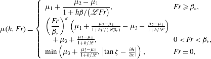 $$\begin{eqnarray}\displaystyle \unicode[STIX]{x1D707}(h,Fr)=\left\{\begin{array}{@{}ll@{}}\displaystyle \unicode[STIX]{x1D707}_{1}+\frac{\unicode[STIX]{x1D707}_{2}-\unicode[STIX]{x1D707}_{1}}{1+h\unicode[STIX]{x1D6FD}/(\mathscr{L}Fr)}, & \displaystyle \!\!Fr\geqslant \unicode[STIX]{x1D6FD}_{\ast },\\ \left({\displaystyle \frac{Fr}{\unicode[STIX]{x1D6FD}_{\ast }}}\right)^{\unicode[STIX]{x1D705}}\left(\unicode[STIX]{x1D707}_{1}+\frac{\unicode[STIX]{x1D707}_{2}-\unicode[STIX]{x1D707}_{1}}{1+h\unicode[STIX]{x1D6FD}/(\mathscr{L}\unicode[STIX]{x1D6FD}_{\ast })}-\unicode[STIX]{x1D707}_{3}-\frac{\unicode[STIX]{x1D707}_{2}-\unicode[STIX]{x1D707}_{1}}{1+h/\mathscr{L}}\right)\\ \quad +\,\unicode[STIX]{x1D707}_{3}+\frac{\unicode[STIX]{x1D707}_{2}-\unicode[STIX]{x1D707}_{1}}{1+h/\mathscr{L}}, & \!\!0<Fr<\unicode[STIX]{x1D6FD}_{\ast },\\ \text{min}\left(\unicode[STIX]{x1D707}_{3}+\frac{\unicode[STIX]{x1D707}_{2}-\unicode[STIX]{x1D707}_{1}}{1+h/\mathscr{L}},\left|\tan \unicode[STIX]{x1D701}-\frac{\unicode[STIX]{x2202}h}{\unicode[STIX]{x2202}x}\right|\right), & \!\!Fr=0,\end{array}\right. & & \displaystyle\end{eqnarray}$$
where
 $\unicode[STIX]{x1D707}_{i}=\tan \unicode[STIX]{x1D701}_{i}$
for
$\unicode[STIX]{x1D707}_{i}=\tan \unicode[STIX]{x1D701}_{i}$
for
 $i=1,2,3$
and the parameters are given in table 1. Importantly, this friction law is identical to that of Pouliquen & Forterre (Reference Pouliquen and Forterre2002) when
$i=1,2,3$
and the parameters are given in table 1. Importantly, this friction law is identical to that of Pouliquen & Forterre (Reference Pouliquen and Forterre2002) when
 $Fr>\unicode[STIX]{x1D6FD}_{\ast }$
, and so is consistent with previous experimental measurements of steady uniform flows (Pouliquen Reference Pouliquen1999a
; Pouliquen & Forterre Reference Pouliquen and Forterre2002).
$Fr>\unicode[STIX]{x1D6FD}_{\ast }$
, and so is consistent with previous experimental measurements of steady uniform flows (Pouliquen Reference Pouliquen1999a
; Pouliquen & Forterre Reference Pouliquen and Forterre2002).
Parameters for the effective basal friction law (3.6)–(3.8) for 125–
 $160~\unicode[STIX]{x03BC}\text{m}$
diameter glass ballotini on a rough bed made of a monolayer of 750–
$160~\unicode[STIX]{x03BC}\text{m}$
diameter glass ballotini on a rough bed made of a monolayer of 750–
 $1000~\unicode[STIX]{x03BC}\text{m}$
diameter glass ballotini. The angles
$1000~\unicode[STIX]{x03BC}\text{m}$
diameter glass ballotini. The angles
 $\unicode[STIX]{x1D701}_{1-3}$
and
$\unicode[STIX]{x1D701}_{1-3}$
and
 $\mathscr{L}$
are fitted from the experimentally measured
$\mathscr{L}$
are fitted from the experimentally measured
 $h_{stop}(\unicode[STIX]{x1D701})$
and
$h_{stop}(\unicode[STIX]{x1D701})$
and
 $h_{start}(\unicode[STIX]{x1D701})$
curves in figure 6,
$h_{start}(\unicode[STIX]{x1D701})$
curves in figure 6,
 $\unicode[STIX]{x1D6FD}$
is taken from Pouliquen (Reference Pouliquen1999a
) with a
$\unicode[STIX]{x1D6FD}$
is taken from Pouliquen (Reference Pouliquen1999a
) with a
 $1/\sqrt{\cos \unicode[STIX]{x1D701}}$
correction, while
$1/\sqrt{\cos \unicode[STIX]{x1D701}}$
correction, while
 $\unicode[STIX]{x1D6FD}_{\ast }$
and
$\unicode[STIX]{x1D6FD}_{\ast }$
and
 $\unicode[STIX]{x1D705}$
are measured using the retrogressive failure experiments in this paper.
$\unicode[STIX]{x1D705}$
are measured using the retrogressive failure experiments in this paper.
The friction law (3.6)–(3.8) encodes information about the empirical flow rule (Pouliquen Reference Pouliquen1999a ; Pouliquen & Forterre Reference Pouliquen and Forterre2002)
 $$\begin{eqnarray}\displaystyle Fr=\unicode[STIX]{x1D6FD}\frac{h}{h_{stop}(\unicode[STIX]{x1D701})}, & & \displaystyle\end{eqnarray}$$
and the
 $h_{stop}$
and
$h_{stop}$
and
 $h_{start}$
curves
$h_{start}$
curves
 $$\begin{eqnarray}\displaystyle & \displaystyle h_{stop}(\unicode[STIX]{x1D701})=\mathscr{L}\left(\frac{\tan \unicode[STIX]{x1D701}_{2}-\tan \unicode[STIX]{x1D701}_{1}}{\tan \unicode[STIX]{x1D701}-\tan \unicode[STIX]{x1D701}_{1}}-1\right),\quad \unicode[STIX]{x1D701}\in [\unicode[STIX]{x1D701}_{1},\unicode[STIX]{x1D701}_{2}], & \displaystyle\end{eqnarray}$$
 $$\begin{eqnarray}\displaystyle & \displaystyle h_{start}(\unicode[STIX]{x1D701})=\mathscr{L}\left(\frac{\tan \unicode[STIX]{x1D701}_{2}-\tan \unicode[STIX]{x1D701}_{1}}{\tan \unicode[STIX]{x1D701}-\tan \unicode[STIX]{x1D701}_{3}}-1\right),\quad \unicode[STIX]{x1D701}\in [\unicode[STIX]{x1D701}_{3},\unicode[STIX]{x1D701}_{4}], & \displaystyle\end{eqnarray}$$
where
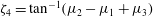 $\unicode[STIX]{x1D701}_{4}=\tan ^{-1}(\unicode[STIX]{x1D707}_{2}-\unicode[STIX]{x1D707}_{1}+\unicode[STIX]{x1D707}_{3})$
. Edwards et al. (Reference Edwards, Russell, Johnson and Gray2019) also introduced the minimum observable steady uniform flow thickness
$\unicode[STIX]{x1D701}_{4}=\tan ^{-1}(\unicode[STIX]{x1D707}_{2}-\unicode[STIX]{x1D707}_{1}+\unicode[STIX]{x1D707}_{3})$
. Edwards et al. (Reference Edwards, Russell, Johnson and Gray2019) also introduced the minimum observable steady uniform flow thickness
 $h_{\ast }$
, which occurs at the transition between the intermediate and dynamic regimes at
$h_{\ast }$
, which occurs at the transition between the intermediate and dynamic regimes at
 $Fr=\unicode[STIX]{x1D6FD}_{\ast }$
. In particular, if
$Fr=\unicode[STIX]{x1D6FD}_{\ast }$
. In particular, if
 $\unicode[STIX]{x1D6FD}_{\ast }$
is constant then the empirical flow rule (3.9) implies that
$\unicode[STIX]{x1D6FD}_{\ast }$
is constant then the empirical flow rule (3.9) implies that
 $h_{\ast }$
is proportional to
$h_{\ast }$
is proportional to
 $h_{stop}$
(Edwards et al.
Reference Edwards, Russell, Johnson and Gray2019)
$h_{stop}$
(Edwards et al.
Reference Edwards, Russell, Johnson and Gray2019)
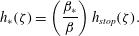 $$\begin{eqnarray}\displaystyle h_{\ast }(\unicode[STIX]{x1D701})=\left(\frac{\unicode[STIX]{x1D6FD}_{\ast }}{\unicode[STIX]{x1D6FD}}\right)h_{stop}(\unicode[STIX]{x1D701}). & & \displaystyle\end{eqnarray}$$
In order to experimentally fit the
 $h_{stop}(\unicode[STIX]{x1D701})$
and
$h_{stop}(\unicode[STIX]{x1D701})$
and
 $h_{start}(\unicode[STIX]{x1D701})$
functions (3.10) and (3.11) a steady uniform flow at an angle
$h_{start}(\unicode[STIX]{x1D701})$
functions (3.10) and (3.11) a steady uniform flow at an angle
 $\unicode[STIX]{x1D701}_{0}$
is created, which leaves behind a deposit of
$\unicode[STIX]{x1D701}_{0}$
is created, which leaves behind a deposit of
 $h_{stop}(\unicode[STIX]{x1D701}_{0})$
. This static layer is then inclined gently to an angle
$h_{stop}(\unicode[STIX]{x1D701}_{0})$
. This static layer is then inclined gently to an angle
 $\unicode[STIX]{x1D701}_{start}=h_{start}^{-1}(h_{stop}(\unicode[STIX]{x1D701}_{0}))>\unicode[STIX]{x1D701}_{0}$
, where it spontaneously starts flowing. There is a large spread in the data for
$\unicode[STIX]{x1D701}_{start}=h_{start}^{-1}(h_{stop}(\unicode[STIX]{x1D701}_{0}))>\unicode[STIX]{x1D701}_{0}$
, where it spontaneously starts flowing. There is a large spread in the data for
 $\unicode[STIX]{x1D701}_{start}$
due to the layer of grains becoming increasingly sensitive to infinitesimal perturbations as it is inclined towards the angle at which it will spontaneously fail. The
$\unicode[STIX]{x1D701}_{start}$
due to the layer of grains becoming increasingly sensitive to infinitesimal perturbations as it is inclined towards the angle at which it will spontaneously fail. The
 $\unicode[STIX]{x1D701}_{start}$
curve is also sensitive to the packing of the grains, which induces some intrinsic variation in the data (Balmforth & McElwaine Reference Balmforth and McElwaine2018). This process is repeated for a range of angles
$\unicode[STIX]{x1D701}_{start}$
curve is also sensitive to the packing of the grains, which induces some intrinsic variation in the data (Balmforth & McElwaine Reference Balmforth and McElwaine2018). This process is repeated for a range of angles
 $\unicode[STIX]{x1D701}_{0}$
to generate the data in figure 6 and hence determine the parameters
$\unicode[STIX]{x1D701}_{0}$
to generate the data in figure 6 and hence determine the parameters
 $\unicode[STIX]{x1D701}_{1}$
,
$\unicode[STIX]{x1D701}_{1}$
,
 $\unicode[STIX]{x1D701}_{2}$
,
$\unicode[STIX]{x1D701}_{2}$
,
 $\unicode[STIX]{x1D701}_{3}$
and
$\unicode[STIX]{x1D701}_{3}$
and
 $\mathscr{L}$
in table 1. In this paper, the value of
$\mathscr{L}$
in table 1. In this paper, the value of
 $\unicode[STIX]{x1D6FD}$
is essentially taken to be the same as the value of 0.136 measured in experiments of Pouliquen (Reference Pouliquen1999a
) for glass ballotini. However, due to Pouliquen’s (Reference Pouliquen1999a
) alternative definition of the Froude number
$\unicode[STIX]{x1D6FD}$
is essentially taken to be the same as the value of 0.136 measured in experiments of Pouliquen (Reference Pouliquen1999a
) for glass ballotini. However, due to Pouliquen’s (Reference Pouliquen1999a
) alternative definition of the Froude number
 $Fr=|\bar{u}|/\sqrt{gh}$
, compared to (3.4), a correction of
$Fr=|\bar{u}|/\sqrt{gh}$
, compared to (3.4), a correction of
 $1/\sqrt{\cos \unicode[STIX]{x1D701}}$
is made, with a typical value of
$1/\sqrt{\cos \unicode[STIX]{x1D701}}$
is made, with a typical value of
 $\unicode[STIX]{x1D701}$
in the range
$\unicode[STIX]{x1D701}$
in the range
 $[22^{\circ },28^{\circ }]$
studied by Pouliquen (Reference Pouliquen1999a
), to give
$[22^{\circ },28^{\circ }]$
studied by Pouliquen (Reference Pouliquen1999a
), to give
 $\unicode[STIX]{x1D6FD}=0.143$
.
$\unicode[STIX]{x1D6FD}=0.143$
.
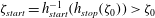
Experimental data for the
 $h_{stop}(\unicode[STIX]{x1D701})$
and
$h_{stop}(\unicode[STIX]{x1D701})$
and
 $h_{start}(\unicode[STIX]{x1D701})$
curves (black and white circles, respectively) and empirical fits (red and green lines, respectively) using equations (3.10) and (3.11) and the parameters in table 1. The experiments are performed with 125–
$h_{start}(\unicode[STIX]{x1D701})$
curves (black and white circles, respectively) and empirical fits (red and green lines, respectively) using equations (3.10) and (3.11) and the parameters in table 1. The experiments are performed with 125–
 $160~\unicode[STIX]{x03BC}\text{m}$
spherical glass ballotini on a monolayer of 750–
$160~\unicode[STIX]{x03BC}\text{m}$
spherical glass ballotini on a monolayer of 750–
 $1000~\unicode[STIX]{x03BC}\text{m}$
spherical glass beads stuck to a wooden surface. The orange line shows the functional form of
$1000~\unicode[STIX]{x03BC}\text{m}$
spherical glass beads stuck to a wooden surface. The orange line shows the functional form of
 $h_{\ast }(\unicode[STIX]{x1D701})$
given by (3.12).
$h_{\ast }(\unicode[STIX]{x1D701})$
given by (3.12).
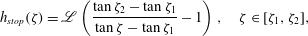
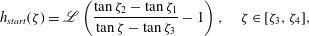
The formula for the intermediate regime (3.7) is a monotonically decreasing function of the Froude number, which interpolates between the maximum static friction
 $\unicode[STIX]{x1D707}_{start}$
and the minimum dynamic friction at
$\unicode[STIX]{x1D707}_{start}$
and the minimum dynamic friction at
 $Fr=\unicode[STIX]{x1D6FD}_{\ast }$
(Pouliquen & Forterre Reference Pouliquen and Forterre2002; Edwards et al.
Reference Edwards, Viroulet, Kokelaar and Gray2017, Reference Edwards, Russell, Johnson and Gray2019). Edwards et al. (Reference Edwards, Viroulet, Kokelaar and Gray2017, Reference Edwards, Russell, Johnson and Gray2019) suggested an interpolation power
$Fr=\unicode[STIX]{x1D6FD}_{\ast }$
(Pouliquen & Forterre Reference Pouliquen and Forterre2002; Edwards et al.
Reference Edwards, Viroulet, Kokelaar and Gray2017, Reference Edwards, Russell, Johnson and Gray2019). Edwards et al. (Reference Edwards, Viroulet, Kokelaar and Gray2017, Reference Edwards, Russell, Johnson and Gray2019) suggested an interpolation power
 $\unicode[STIX]{x1D705}=1$
in (3.7) to give static material in the metastable range of thicknesses greater stability to small perturbations than in Pouliquen & Forterre’s (Reference Pouliquen and Forterre2002) original formulation. Pouliquen & Forterre (Reference Pouliquen and Forterre2002) used a value of
$\unicode[STIX]{x1D705}=1$
in (3.7) to give static material in the metastable range of thicknesses greater stability to small perturbations than in Pouliquen & Forterre’s (Reference Pouliquen and Forterre2002) original formulation. Pouliquen & Forterre (Reference Pouliquen and Forterre2002) used a value of
 $\unicode[STIX]{x1D705}=10^{-3}$
instead, which implies that the hysteretic friction is only partially represented in typical machine precision calculations (Edwards et al.
Reference Edwards, Russell, Johnson and Gray2019) and as a result, the metastable range of thicknesses
$\unicode[STIX]{x1D705}=10^{-3}$
instead, which implies that the hysteretic friction is only partially represented in typical machine precision calculations (Edwards et al.
Reference Edwards, Russell, Johnson and Gray2019) and as a result, the metastable range of thicknesses
 $[h_{\ast },h_{start}]$
is much more sensitive to disturbances than is physically realistic.
$[h_{\ast },h_{start}]$
is much more sensitive to disturbances than is physically realistic.
For the glass beads in our experiments, the slowest steady uniform flows attainable are at
 $h_{\ast }/h_{stop}=1.33$
, which by (3.12) implies
$h_{\ast }/h_{stop}=1.33$
, which by (3.12) implies
 $\unicode[STIX]{x1D6FD}_{\ast }=0.19$
and hence that
$\unicode[STIX]{x1D6FD}_{\ast }=0.19$
and hence that
 $h_{\ast }\in (h_{stop},h_{start})$
for all angles in
$h_{\ast }\in (h_{stop},h_{start})$
for all angles in
 $[\unicode[STIX]{x1D701}_{1},\unicode[STIX]{x1D701}_{2}]$
. The friction transition at
$[\unicode[STIX]{x1D701}_{1},\unicode[STIX]{x1D701}_{2}]$
. The friction transition at
 $Fr=\unicode[STIX]{x1D6FD}_{\ast }$
implies the minimum steady uniform flow thickness
$Fr=\unicode[STIX]{x1D6FD}_{\ast }$
implies the minimum steady uniform flow thickness
 $h_{\ast }>h_{stop}$
, contrary to Pouliquen & Forterre’s (Reference Pouliquen and Forterre2002) original hypothesis that the minimum steady uniform flow thickness
$h_{\ast }>h_{stop}$
, contrary to Pouliquen & Forterre’s (Reference Pouliquen and Forterre2002) original hypothesis that the minimum steady uniform flow thickness
 $h_{stop}$
occurred at
$h_{stop}$
occurred at
 $Fr=\unicode[STIX]{x1D6FD}$
. Edwards et al. (Reference Edwards, Viroulet, Kokelaar and Gray2017, Reference Edwards, Russell, Johnson and Gray2019) showed, however, that modifying the transition in this way implied that a steady uniform flow close to
$Fr=\unicode[STIX]{x1D6FD}$
. Edwards et al. (Reference Edwards, Viroulet, Kokelaar and Gray2017, Reference Edwards, Russell, Johnson and Gray2019) showed, however, that modifying the transition in this way implied that a steady uniform flow close to
 $h_{\ast }$
produced a deposit depth close to
$h_{\ast }$
produced a deposit depth close to
 $h_{stop}$
as observed in experiment, whilst Pouliquen & Forterre’s (Reference Pouliquen and Forterre2002) transition produced deposits that were thinner than
$h_{stop}$
as observed in experiment, whilst Pouliquen & Forterre’s (Reference Pouliquen and Forterre2002) transition produced deposits that were thinner than
 $h_{stop}$
(see e.g. Edwards & Gray Reference Edwards and Gray2015).
$h_{stop}$
(see e.g. Edwards & Gray Reference Edwards and Gray2015).
4 Numerical simulations of retrogressive failure
Retrogressive failure fronts are simulated by solving the conservation laws (3.1)–(3.2) together with the friction law (3.6)–(3.8) numerically. The central scheme of Kurganov & Tadmor (Reference Kurganov and Tadmor2000) and a second-order Runge–Kutta method are used to discretise the equations, with the time step determined by a Courant–Friedrichs–Lewy (CFL) number of
 $1/4$
. In static regions, the equilibrium force balance is assessed prior to each time step and the friction coefficient set appropriately using (3.8), resulting in a well-balanced discretisation of the source terms that preserves these static states exactly. The material parameter values used in these numerical simulations are given in table 1.
$1/4$
. In static regions, the equilibrium force balance is assessed prior to each time step and the friction coefficient set appropriately using (3.8), resulting in a well-balanced discretisation of the source terms that preserves these static states exactly. The material parameter values used in these numerical simulations are given in table 1.
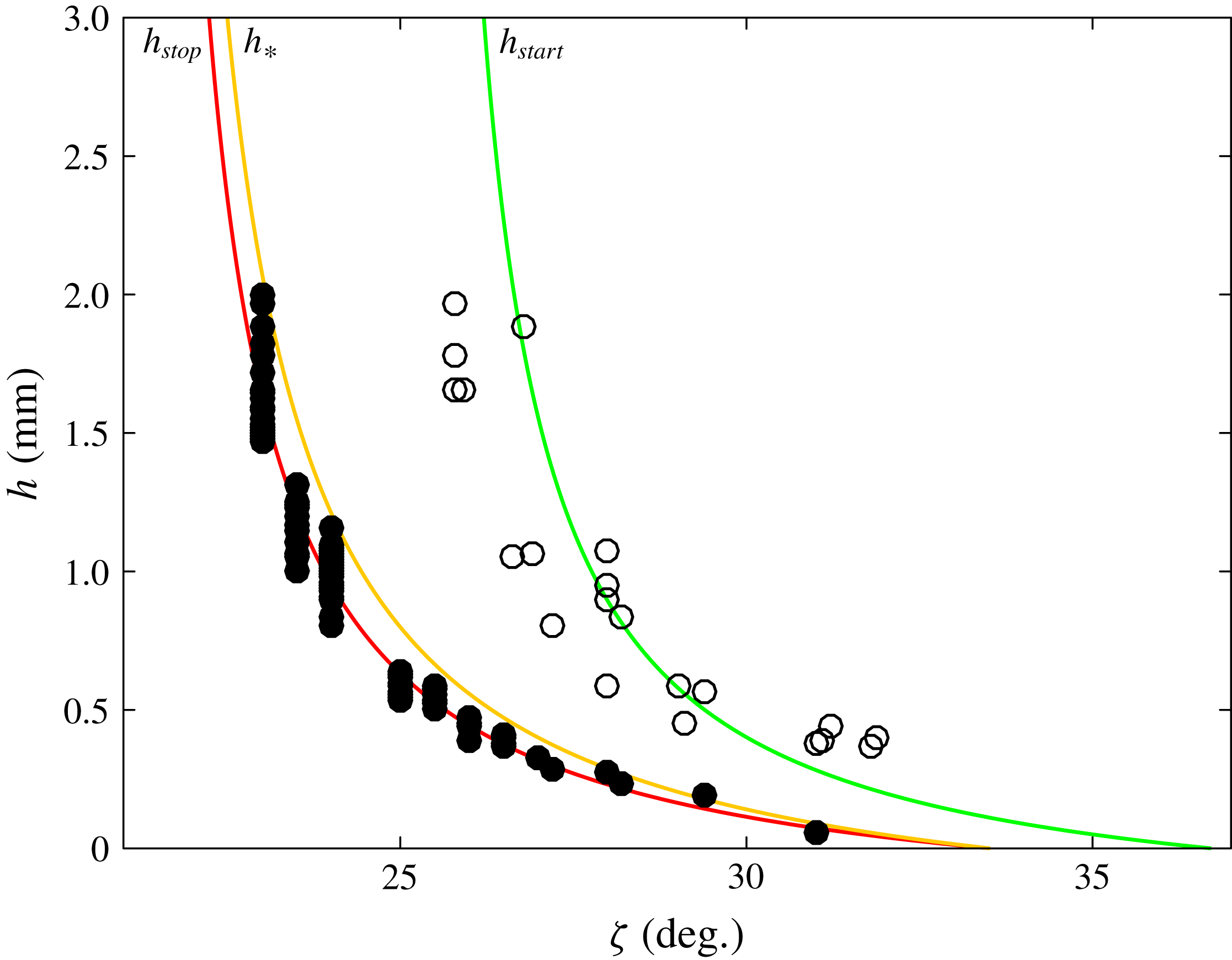
The retrogressive wave thickness
 $h(x,t)$
and downslope velocity
$h(x,t)$
and downslope velocity
 $u(x,z,t)$
at a sequence of time steps (a) 0 s (b) 0.15 s (c) 0.3 s (d) 0.45 s and (e) 0.6 s for a slope inclined at
$u(x,z,t)$
at a sequence of time steps (a) 0 s (b) 0.15 s (c) 0.3 s (d) 0.45 s and (e) 0.6 s for a slope inclined at
 $\unicode[STIX]{x1D701}=27.5^{\circ }$
. The initial stationary layer is of thickness
$\unicode[STIX]{x1D701}=27.5^{\circ }$
. The initial stationary layer is of thickness
 $h(x,0)=1.0$
mm. The filled region shows the thickness and the contour scale within it denotes the velocity, which is reconstructed from the depth-averaged downslope velocity
$h(x,0)=1.0$
mm. The filled region shows the thickness and the contour scale within it denotes the velocity, which is reconstructed from the depth-averaged downslope velocity
 $\bar{u}(x,t)$
assuming an exponential profile (4.1) with
$\bar{u}(x,t)$
assuming an exponential profile (4.1) with
 $\unicode[STIX]{x1D706}=2.45$
. There is no inflow at
$\unicode[STIX]{x1D706}=2.45$
. There is no inflow at
 $x=0$
and there is free outflow at the downstream boundary. The diagonal dashed line shows that the retrogressive failure front rapidly develops and travels upslope at a constant speed. The wave erodes the static surface particles, which are shown with light blue markers and they travel downslope on the surface of the steady uniform flow. The material properties are given in table 1 and an animation is shown in movie 5 of the online supplementary material.
$x=0$
and there is free outflow at the downstream boundary. The diagonal dashed line shows that the retrogressive failure front rapidly develops and travels upslope at a constant speed. The wave erodes the static surface particles, which are shown with light blue markers and they travel downslope on the surface of the steady uniform flow. The material properties are given in table 1 and an animation is shown in movie 5 of the online supplementary material.
A solution exhibiting retrogressive failure on a slope inclined at
 $\unicode[STIX]{x1D701}=27.5^{\circ }$
is shown in figure 7 and supplementary movie 5. Initially for
$\unicode[STIX]{x1D701}=27.5^{\circ }$
is shown in figure 7 and supplementary movie 5. Initially for
 $x<0.06$
m there is a stationary layer of thickness
$x<0.06$
m there is a stationary layer of thickness
 $h(x,0)=1.0$
mm and for
$h(x,0)=1.0$
mm and for
 $x>0.06$
m the chute is empty. There is no inflow at
$x>0.06$
m the chute is empty. There is no inflow at
 $x=0$
and free outflow at the downstream boundary. A retrogressive failure wave rapidly develops (figure 7
b) and travels upslope at a constant speed (figure 7
b–e, indicated by the dashed line). This wave connects a thicker static deposit upslope and thinner flowing region downslope.
$x=0$
and free outflow at the downstream boundary. A retrogressive failure wave rapidly develops (figure 7
b) and travels upslope at a constant speed (figure 7
b–e, indicated by the dashed line). This wave connects a thicker static deposit upslope and thinner flowing region downslope.
The two-dimensional downslope velocity field
 $u(x,z,t)$
is reconstructed from the depth-averaged downslope velocity
$u(x,z,t)$
is reconstructed from the depth-averaged downslope velocity
 $\bar{u}(x,t)$
assuming an exponential velocity profile through the depth of the avalanche as in Wiederseiner et al. (Reference Wiederseiner, Andreini, Epely-Chauvin, Moser, Monnereau, Gray and Ancey2011),
$\bar{u}(x,t)$
assuming an exponential velocity profile through the depth of the avalanche as in Wiederseiner et al. (Reference Wiederseiner, Andreini, Epely-Chauvin, Moser, Monnereau, Gray and Ancey2011),
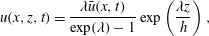 $$\begin{eqnarray}\displaystyle u(x,z,t)=\frac{\unicode[STIX]{x1D706}\bar{u}(x,t)}{\exp (\unicode[STIX]{x1D706})-1}\exp \left(\frac{\unicode[STIX]{x1D706}z}{h}\right), & & \displaystyle\end{eqnarray}$$
where the non-dimensional parameter
 $\unicode[STIX]{x1D706}$
determines the ratio of surface to depth-averaged velocity,
$\unicode[STIX]{x1D706}$
determines the ratio of surface to depth-averaged velocity,
 $$\begin{eqnarray}\displaystyle \frac{u_{s}}{\bar{u}}=\frac{\unicode[STIX]{x1D706}\exp (\unicode[STIX]{x1D706})}{\exp (\unicode[STIX]{x1D706})-1}. & & \displaystyle\end{eqnarray}$$
Concave velocity profiles of this sort are predicted for shallow flows by the non-local rheology of Kamrin & Henann (Reference Kamrin and Henann2015) and by discrete element simulations (their figure 2).
The parameter
 $\unicode[STIX]{x1D706}$
is calibrated experimentally by creating a static layer at an angle
$\unicode[STIX]{x1D706}$
is calibrated experimentally by creating a static layer at an angle
 $\unicode[STIX]{x1D701}_{0}$
, placing a ruler across the deposit and sweeping the grains off the chute downslope of the ruler. The chute was then inclined to an angle
$\unicode[STIX]{x1D701}_{0}$
, placing a ruler across the deposit and sweeping the grains off the chute downslope of the ruler. The chute was then inclined to an angle
 $\unicode[STIX]{x1D701}>\unicode[STIX]{x1D701}_{0}$
and the ruler was then removed, allowing a retrogressive failure to propagate upslope through the static layer of grains. Downstream of the release a steady uniform flow rapidly developed with a granular front (Pouliquen Reference Pouliquen1999b
) that propagated downslope with the depth-averaged speed of the flow. Both the surface velocity
$\unicode[STIX]{x1D701}>\unicode[STIX]{x1D701}_{0}$
and the ruler was then removed, allowing a retrogressive failure to propagate upslope through the static layer of grains. Downstream of the release a steady uniform flow rapidly developed with a granular front (Pouliquen Reference Pouliquen1999b
) that propagated downslope with the depth-averaged speed of the flow. Both the surface velocity
 $u_{s}$
of the uniform flow and the speed of the granular front
$u_{s}$
of the uniform flow and the speed of the granular front
 $\bar{u}$
were measured, and (4.2) was used to determine
$\bar{u}$
were measured, and (4.2) was used to determine
 $\unicode[STIX]{x1D706}$
. For experimental conditions close to those in figure 4 the surface velocity
$\unicode[STIX]{x1D706}$
. For experimental conditions close to those in figure 4 the surface velocity
 $u_{s}=8.5~\text{cm}~\text{s}^{-1}$
and
$u_{s}=8.5~\text{cm}~\text{s}^{-1}$
and
 $\bar{u}=3.2~\text{cm}~\text{s}^{-1}$
, giving
$\bar{u}=3.2~\text{cm}~\text{s}^{-1}$
, giving
 $u_{s}/\bar{u}=2.7$
and hence
$u_{s}/\bar{u}=2.7$
and hence
 $\unicode[STIX]{x1D706}=2.45$
. This reconstruction allows integration of surface particle trajectories (light blue markers in figure 7). As the particles accelerate and the flow thins, the spacing between the particles increases. An animation showing how the particles move at different depths in the flow (movie 6) is available in the online supplementary material.
$\unicode[STIX]{x1D706}=2.45$
. This reconstruction allows integration of surface particle trajectories (light blue markers in figure 7). As the particles accelerate and the flow thins, the spacing between the particles increases. An animation showing how the particles move at different depths in the flow (movie 6) is available in the online supplementary material.
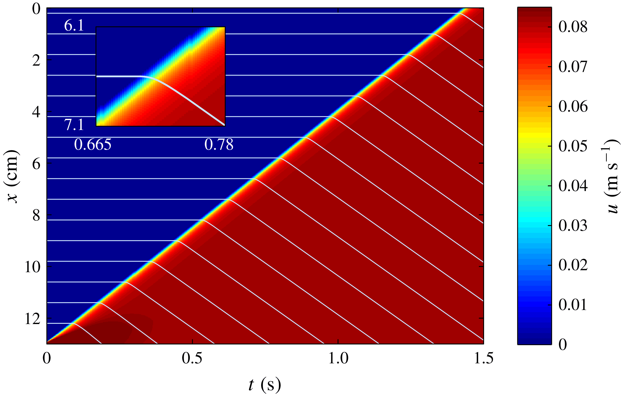
The downslope surface velocity can also be visualised in a space–time plot (figure 8). The contours of
 $u_{s}$
form parallel diagonal lines, indicating the rapid development of a travelling retrogressive failure that moves upslope at a constant speed. A series of particle trajectories are plotted on top of the contours (light blue lines), with stationary particles upslope of the failure (horizontal lines) and moving particles downslope (diagonal lines). This is the same behaviour shown in the experimental space–time plot in figure 4. The simulated retrogressive wave speed of
$u_{s}$
form parallel diagonal lines, indicating the rapid development of a travelling retrogressive failure that moves upslope at a constant speed. A series of particle trajectories are plotted on top of the contours (light blue lines), with stationary particles upslope of the failure (horizontal lines) and moving particles downslope (diagonal lines). This is the same behaviour shown in the experimental space–time plot in figure 4. The simulated retrogressive wave speed of
 $9.1~\text{cm}~\text{s}^{-1}$
is similar to the experimentally measured wave speed
$9.1~\text{cm}~\text{s}^{-1}$
is similar to the experimentally measured wave speed
 $|u_{w}|=8.5~\text{cm}~\text{s}^{-1}$
, while the simulated surface velocity of the steady uniform flow downstream of the failure
$|u_{w}|=8.5~\text{cm}~\text{s}^{-1}$
, while the simulated surface velocity of the steady uniform flow downstream of the failure
 $u_{s}=8.1~\text{cm}~\text{s}^{-1}$
is within
$u_{s}=8.1~\text{cm}~\text{s}^{-1}$
is within
 $0.1~\text{cm}~\text{s}^{-1}$
of that measured in the experiment.
$0.1~\text{cm}~\text{s}^{-1}$
of that measured in the experiment.
Space–time
 $(t,x)$
plot showing the surface velocity
$(t,x)$
plot showing the surface velocity
 $u(x,h,t)$
of a retrogressive failure front on a slope inclined at
$u(x,h,t)$
of a retrogressive failure front on a slope inclined at
 $\unicode[STIX]{x1D701}=27.5^{\circ }$
with an initial stationary layer of thickness
$\unicode[STIX]{x1D701}=27.5^{\circ }$
with an initial stationary layer of thickness
 $h(x,0)=1.0$
mm. Individual surface particles are tracked (light blue lines) to visualise the particle trajectories through the retrogressive failure front. The horizontal lines indicate stationary particles and the diagonal lines represent moving surface particles whose velocity is reconstructed assuming an exponential profile (4.1) with
$h(x,0)=1.0$
mm. Individual surface particles are tracked (light blue lines) to visualise the particle trajectories through the retrogressive failure front. The horizontal lines indicate stationary particles and the diagonal lines represent moving surface particles whose velocity is reconstructed assuming an exponential profile (4.1) with
 $\unicode[STIX]{x1D706}=2.45$
. The inset shows a close up of one of the particle paths as it goes through the retrogressive failure front. The material properties are given in table 1.
$\unicode[STIX]{x1D706}=2.45$
. The inset shows a close up of one of the particle paths as it goes through the retrogressive failure front. The material properties are given in table 1.
5 Travelling wave solutions for retrogressive failure
The experiments in § 2 and the numerical simulations in § 4 suggest that retrogressive failures rapidly develop into travelling waves. This is now investigated, within the framework of the avalanche model described in § 3, by using a travelling wave ansatz.
5.1 Equations in a steadily moving frame
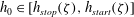
A schematic diagram of the anticipated solution structure is shown in figure 1. It consists of a static region of constant thickness
 $h_{0}$
, that lies upstream of a flowing region, which decreases in thickness as it accelerates towards a steady uniform flow of thickness
$h_{0}$
, that lies upstream of a flowing region, which decreases in thickness as it accelerates towards a steady uniform flow of thickness
 $h_{\infty }<h_{0}$
and depth-averaged velocity
$h_{\infty }<h_{0}$
and depth-averaged velocity
 $\bar{u}_{\infty }$
. The retrogressive failure is assumed to travel upslope with velocity
$\bar{u}_{\infty }$
. The retrogressive failure is assumed to travel upslope with velocity
 $u_{w}<0$
. Looking for steady solutions in the frame of the retrogressive wave
$u_{w}<0$
. Looking for steady solutions in the frame of the retrogressive wave
 $\unicode[STIX]{x1D709}=x-u_{w}t$
, the governing equations (3.1)–(3.2) reduce to
$\unicode[STIX]{x1D709}=x-u_{w}t$
, the governing equations (3.1)–(3.2) reduce to
 $$\begin{eqnarray}\displaystyle & \displaystyle \frac{\text{d}}{\text{d}\unicode[STIX]{x1D709}}(h(\bar{u}-u_{w}))=0, & \displaystyle\end{eqnarray}$$
 $$\begin{eqnarray}\displaystyle & \displaystyle (\bar{u}-u_{w})\frac{\text{d}\bar{u}}{\text{d}\unicode[STIX]{x1D709}}+g\cos \unicode[STIX]{x1D701}\frac{\text{d}h}{\text{d}\unicode[STIX]{x1D709}}=gS\cos \unicode[STIX]{x1D701}, & \displaystyle\end{eqnarray}$$
where the acceleration terms in (5.2) have been simplified using (5.1). Integrating the mass balance (5.1) with respect to
 $\unicode[STIX]{x1D709}$
, subject to the condition that the thickness is constant
$\unicode[STIX]{x1D709}$
, subject to the condition that the thickness is constant
 $h=h_{0}$
and
$h=h_{0}$
and
 $\bar{u}=0$
in the static region, implies that the flux in the moving frame is constant
$\bar{u}=0$
in the static region, implies that the flux in the moving frame is constant
 $$\begin{eqnarray}\displaystyle h(\bar{u}-u_{w})=-u_{w}h_{0}. & & \displaystyle\end{eqnarray}$$
This can be rearranged to show that the depth-averaged velocity, anywhere in the flow, is a function of the wave velocity and thickness
 $$\begin{eqnarray}\displaystyle \bar{u}=u_{w}\left(1-\frac{h_{0}}{h}\right). & & \displaystyle\end{eqnarray}$$
Substituting for the depth-averaged velocity in (5.2) and using (5.3) to simplify the result, implies that the thickness profile satisfies the autonomous ordinary differential equation (ODE)
 $$\begin{eqnarray}\displaystyle \frac{\text{d}h}{\text{d}\unicode[STIX]{x1D709}}=\frac{S(h)}{1-\displaystyle \frac{u_{w}^{2}h_{0}^{2}}{gh^{3}\cos \unicode[STIX]{x1D701}}}, & & \displaystyle\end{eqnarray}$$
where
 $S(h)=\tan \unicode[STIX]{x1D701}-\unicode[STIX]{x1D707}(h,Fr(h))$
is defined in (3.5) and the Froude number can be written using (3.4) and (5.4) in terms of the thickness, initial thickness and wave speed, as
$S(h)=\tan \unicode[STIX]{x1D701}-\unicode[STIX]{x1D707}(h,Fr(h))$
is defined in (3.5) and the Froude number can be written using (3.4) and (5.4) in terms of the thickness, initial thickness and wave speed, as
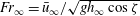
 $$\begin{eqnarray}\displaystyle Fr=\frac{-u_{w}}{\sqrt{gh\cos \unicode[STIX]{x1D701}}}\left(\frac{h_{0}}{h}-1\right). & & \displaystyle\end{eqnarray}$$
The initial layer depth
 $h_{0}$
and the inclination
$h_{0}$
and the inclination
 $\unicode[STIX]{x1D701}$
are prescribed in experiments, so equation (5.5) is a first-order ODE for
$\unicode[STIX]{x1D701}$
are prescribed in experiments, so equation (5.5) is a first-order ODE for
 $h$
with the wave velocity
$h$
with the wave velocity
 $u_{w}$
a free parameter. As the flow thins from the initial thickness
$u_{w}$
a free parameter. As the flow thins from the initial thickness
 $h_{0}$
to the steady uniform thickness
$h_{0}$
to the steady uniform thickness
 $h_{\infty }$
the Froude number increases from zero to the steady uniform flow Froude number
$h_{\infty }$
the Froude number increases from zero to the steady uniform flow Froude number
 $Fr_{\infty }=\bar{u}_{\infty }/\sqrt{gh_{\infty }\cos \unicode[STIX]{x1D701}}$
. This must lie in the dynamic frictional regime, since steady uniform flows in the intermediate regime are unstable. However, in order to connect the static and dynamic equilibria the solution passes through a point where
$Fr_{\infty }=\bar{u}_{\infty }/\sqrt{gh_{\infty }\cos \unicode[STIX]{x1D701}}$
. This must lie in the dynamic frictional regime, since steady uniform flows in the intermediate regime are unstable. However, in order to connect the static and dynamic equilibria the solution passes through a point where
 $S=0$
in the intermediate regime (illustrated in figure 9); this must necessarily occur since the Froude number (5.6) is a strictly decreasing function of
$S=0$
in the intermediate regime (illustrated in figure 9); this must necessarily occur since the Froude number (5.6) is a strictly decreasing function of
 $h$
. If the denominator on the right-hand side of (5.5) is non-zero, solutions to the ODE (5.5) have zero gradient where
$h$
. If the denominator on the right-hand side of (5.5) is non-zero, solutions to the ODE (5.5) have zero gradient where
 $S=0$
, preventing a solution that connects the static and dynamic equilibrium solutions. Consequently, the denominator must be zero when
$S=0$
, preventing a solution that connects the static and dynamic equilibrium solutions. Consequently, the denominator must be zero when
 $S=0$
in the intermediate regime, forming a critical point of the ODE at
$S=0$
in the intermediate regime, forming a critical point of the ODE at
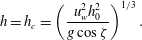 $$\begin{eqnarray}\displaystyle h=h_{c}=\left(\frac{u_{w}^{2}h_{0}^{2}}{g\cos \unicode[STIX]{x1D701}}\right)^{1/3}. & & \displaystyle\end{eqnarray}$$
Writing the ODE (5.5) as
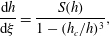 $$\begin{eqnarray}\displaystyle \frac{\text{d}h}{\text{d}\unicode[STIX]{x1D709}}=\frac{S(h)}{1-(h_{c}/h)^{3}}, & & \displaystyle\end{eqnarray}$$
and using L’Hôpital’s rule gives a finite value for the gradient at the critical point,
 $$\begin{eqnarray}\displaystyle \left.\frac{\text{d}h}{\text{d}\unicode[STIX]{x1D709}}\right|_{h=h_{c}}=\frac{h_{c}}{3}\left.\frac{\text{d}S}{\text{d}h}\right|_{h=h_{c}}. & & \displaystyle\end{eqnarray}$$
Contour
 $S=0$
(thick black line) as a function of the Froude number
$S=0$
(thick black line) as a function of the Froude number
 $Fr$
and the thickness
$Fr$
and the thickness
 $h$
for a slope angle
$h$
for a slope angle
 $\unicode[STIX]{x1D701}=26.5^{\circ }$
. In the blue shaded region a constant depth flow is accelerative (
$\unicode[STIX]{x1D701}=26.5^{\circ }$
. In the blue shaded region a constant depth flow is accelerative (
 $S>0$
), in the white region it is decelerative (
$S>0$
), in the white region it is decelerative (
 $S<0$
) and on the zero contour (
$S<0$
) and on the zero contour (
 $S=0$
) it moves at constant speed. The green line is
$S=0$
) it moves at constant speed. The green line is
 $h_{start}$
, the orange line is
$h_{start}$
, the orange line is
 $h_{\ast }$
and the red line is
$h_{\ast }$
and the red line is
 $h_{stop}$
. The vertical dashed line lies at
$h_{stop}$
. The vertical dashed line lies at
 $Fr=\unicode[STIX]{x1D6FD}_{\ast }$
, which is where the friction switches from the intermediate to the dynamic regime. The blue lines show solutions to the ODE (5.5) for different initial layer thicknesses
$Fr=\unicode[STIX]{x1D6FD}_{\ast }$
, which is where the friction switches from the intermediate to the dynamic regime. The blue lines show solutions to the ODE (5.5) for different initial layer thicknesses
 $h_{0}$
and which are parameterised by the curve (5.6) with different values of
$h_{0}$
and which are parameterised by the curve (5.6) with different values of
 $u_{w}$
. The white circles are the critical points, the grey circles are the transitions to static friction, the black circles are the transitions to dynamic friction and the white circles containing the crosses are the steady uniform flow velocities downstream (
$u_{w}$
. The white circles are the critical points, the grey circles are the transitions to static friction, the black circles are the transitions to dynamic friction and the white circles containing the crosses are the steady uniform flow velocities downstream (
 $h_{\infty }$
,
$h_{\infty }$
,
 $\bar{u}_{\infty }$
).
$\bar{u}_{\infty }$
).
Although
 $h_{0}$
is given, it is easiest to solve the problem by assuming a value of the critical thickness
$h_{0}$
is given, it is easiest to solve the problem by assuming a value of the critical thickness
 $h_{c}$
and then solving for
$h_{c}$
and then solving for
 $h_{c}=h_{c}(h_{0})$
later. Assuming that
$h_{c}=h_{c}(h_{0})$
later. Assuming that
 $h_{c}$
is given, the critical Froude number at
$h_{c}$
is given, the critical Froude number at
 $h=h_{c}$
, can be found by solving
$h=h_{c}$
, can be found by solving
 $S=0$
using (3.5) and the intermediate friction law (3.7) to give
$S=0$
using (3.5) and the intermediate friction law (3.7) to give
 $$\begin{eqnarray}\displaystyle Fr_{c}=\unicode[STIX]{x1D6FD}_{\ast }\left[\displaystyle \frac{\tan \unicode[STIX]{x1D701}-\unicode[STIX]{x1D707}_{3}-\displaystyle \frac{\unicode[STIX]{x1D707}_{2}-\unicode[STIX]{x1D707}_{1}}{1+h_{c}/\mathscr{L}}}{\unicode[STIX]{x1D707}_{1}+\displaystyle \frac{\unicode[STIX]{x1D707}_{2}-\unicode[STIX]{x1D707}_{1}}{1+h_{c}\unicode[STIX]{x1D6FD}/\mathscr{L}\unicode[STIX]{x1D6FD}_{\ast }}-\unicode[STIX]{x1D707}_{3}-\displaystyle \frac{\unicode[STIX]{x1D707}_{2}-\unicode[STIX]{x1D707}_{1}}{1+h_{c}/\mathscr{L}}}\right]^{1/\unicode[STIX]{x1D705}}. & & \displaystyle\end{eqnarray}$$
From the definition of the Froude number (3.4) it follows that the critical velocity
 $$\begin{eqnarray}\displaystyle \bar{u}_{c}=Fr_{c}\sqrt{gh_{c}\cos \unicode[STIX]{x1D701}}. & & \displaystyle\end{eqnarray}$$
Substituting
 $h_{c}$
and
$h_{c}$
and
 $\bar{u}_{c}$
into the integrated mass balance (5.3) implies that
$\bar{u}_{c}$
into the integrated mass balance (5.3) implies that
 $$\begin{eqnarray}\displaystyle h_{0}u_{w}=h_{c}(u_{w}-\bar{u}_{c}). & & \displaystyle\end{eqnarray}$$
Solving (5.7) gives another expression for
 $h_{0}u_{w}$
,
$h_{0}u_{w}$
,
 $$\begin{eqnarray}\displaystyle h_{0}u_{w}=-h_{c}\sqrt{gh_{c}\cos \unicode[STIX]{x1D701}}, & & \displaystyle\end{eqnarray}$$
where the negative root in the quadratic is assumed, so that
 $u_{w}$
is negative. Equating (5.12) and (5.13) then determines the velocity of the retrogressive wave
$u_{w}$
is negative. Equating (5.12) and (5.13) then determines the velocity of the retrogressive wave
 $$\begin{eqnarray}\displaystyle u_{w}=\bar{u}_{c}-\sqrt{gh_{c}\cos \unicode[STIX]{x1D701}}, & & \displaystyle\end{eqnarray}$$
which is equal to the upward characteristic velocity (3.3) evaluated at the critical point. Substituting the wave velocity (5.14) back into (5.13) and dividing by
 $\sqrt{gh_{c}\cos \unicode[STIX]{x1D701}}$
then determines the corresponding initial deposit thickness
$\sqrt{gh_{c}\cos \unicode[STIX]{x1D701}}$
then determines the corresponding initial deposit thickness
 $$\begin{eqnarray}\displaystyle h_{0}=\frac{h_{c}}{1-Fr_{c}}. & & \displaystyle\end{eqnarray}$$
If, as in the experiment, the initial deposit thickness
 $h_{0}$
is known but
$h_{0}$
is known but
 $h_{c}$
is not,
$h_{c}$
is not,
 $h_{c}$
can be found by inverting (5.15) numerically with
$h_{c}$
can be found by inverting (5.15) numerically with
 $Fr_{c}(h_{c})$
evaluated using (5.10). For a given value of the thickness
$Fr_{c}(h_{c})$
evaluated using (5.10). For a given value of the thickness
 $h_{c}$
, it follows that the Froude number
$h_{c}$
, it follows that the Froude number
 $Fr_{c}$
, the velocity at the critical point
$Fr_{c}$
, the velocity at the critical point
 $\bar{u}_{c}$
, the wave velocity
$\bar{u}_{c}$
, the wave velocity
 $u_{w}$
and the initial deposit thickness
$u_{w}$
and the initial deposit thickness
 $h_{0}$
are determined by (5.10), (5.11), (5.14) and (5.15), respectively. The thickness profile
$h_{0}$
are determined by (5.10), (5.11), (5.14) and (5.15), respectively. The thickness profile
 $h(\unicode[STIX]{x1D709})$
can then be calculated by numerically integrating (5.8) upslope from
$h(\unicode[STIX]{x1D709})$
can then be calculated by numerically integrating (5.8) upslope from
 $h_{c}$
to
$h_{c}$
to
 $h_{0}$
and downslope from
$h_{0}$
and downslope from
 $h_{c}$
to
$h_{c}$
to
 $h_{\infty }$
, using L’Hôpital’s rule (5.9) to start the integration.
$h_{\infty }$
, using L’Hôpital’s rule (5.9) to start the integration.
A series of retrogressive travelling wave solutions for (a) the thickness
 $h$
and (b) the depth-averaged downslope velocity
$h$
and (b) the depth-averaged downslope velocity
 $\bar{u}$
as a function of the travelling wave coordinate
$\bar{u}$
as a function of the travelling wave coordinate
 $\unicode[STIX]{x1D709}$
and for an inclination
$\unicode[STIX]{x1D709}$
and for an inclination
 $\unicode[STIX]{x1D701}=26.5^{\circ }$
. The solutions correspond to an initial layer thicknesses
$\unicode[STIX]{x1D701}=26.5^{\circ }$
. The solutions correspond to an initial layer thicknesses
 $h_{0}=h_{stop}(22.55^{\circ }),h_{stop}(23^{\circ }),h_{stop}(23.5^{\circ }),h_{stop}(24^{\circ }),h_{stop}(25.068^{\circ })$
, with the thicker layers corresponding to
$h_{0}=h_{stop}(22.55^{\circ }),h_{stop}(23^{\circ }),h_{stop}(23.5^{\circ }),h_{stop}(24^{\circ }),h_{stop}(25.068^{\circ })$
, with the thicker layers corresponding to
 $h_{stop}$
at lower angles. The point at which static material is mobilised by the wave at
$h_{stop}$
at lower angles. The point at which static material is mobilised by the wave at
 $\unicode[STIX]{x1D709}=0$
is indicated by a grey filled circle, the critical point
$\unicode[STIX]{x1D709}=0$
is indicated by a grey filled circle, the critical point
 $h=h_{c}$
by a white filled circle, the transition to dynamic friction at
$h=h_{c}$
by a white filled circle, the transition to dynamic friction at
 $Fr=\unicode[STIX]{x1D6FD}_{\ast }$
by a black circle and the steady uniform flow downstream (
$Fr=\unicode[STIX]{x1D6FD}_{\ast }$
by a black circle and the steady uniform flow downstream (
 $h=h_{\infty }$
,
$h=h_{\infty }$
,
 $\bar{u}=\bar{u}_{\infty }$
) by a crossed circle. The deeper steady uniform flows in (a) correspond to faster depth-averaged velocities in (b) and there is no motion for
$\bar{u}=\bar{u}_{\infty }$
) by a crossed circle. The deeper steady uniform flows in (a) correspond to faster depth-averaged velocities in (b) and there is no motion for
 $\unicode[STIX]{x1D709}<0$
.
$\unicode[STIX]{x1D709}<0$
.
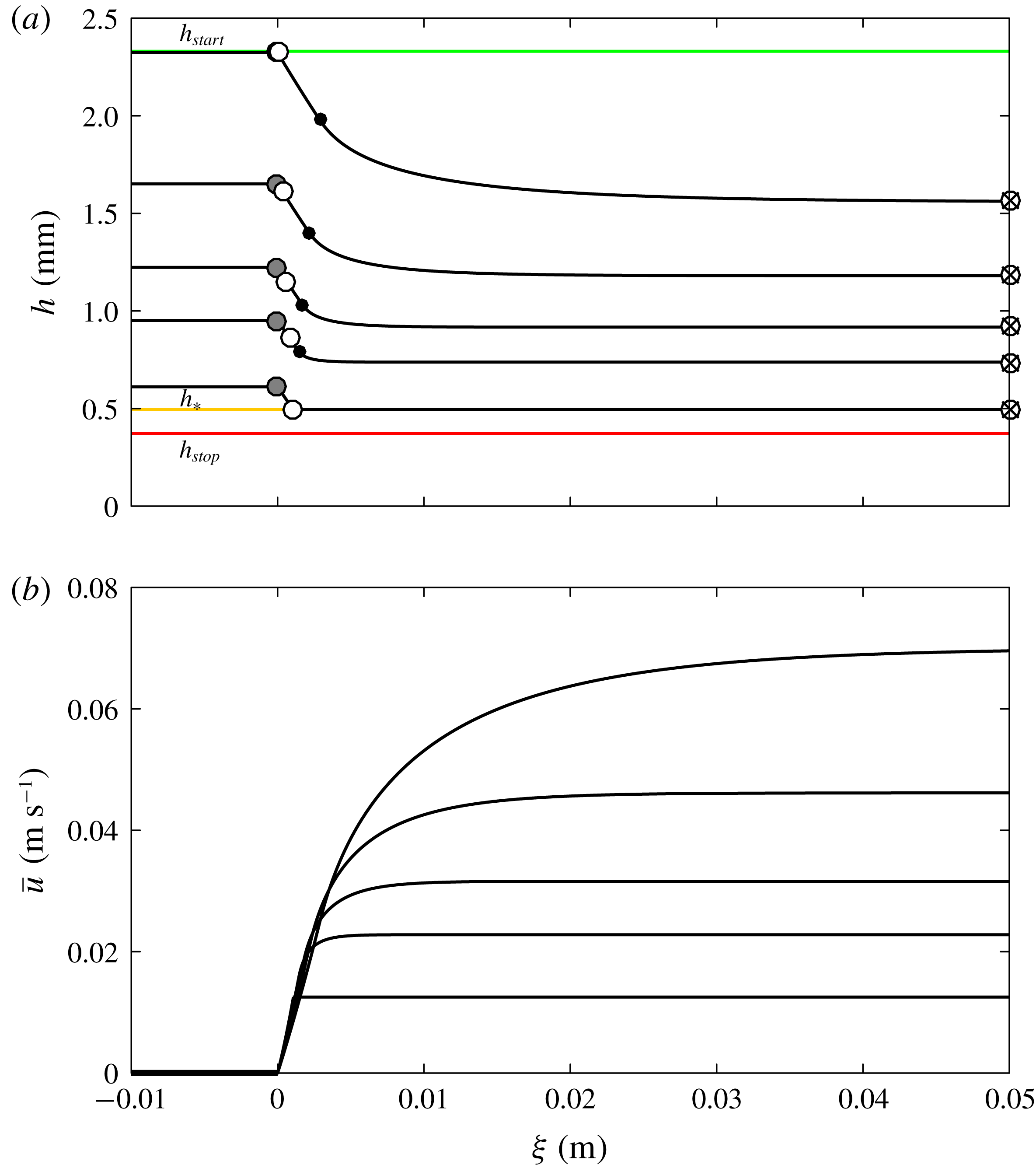
A series of thickness profiles for different static deposit thicknesses
 $h_{0}$
and for
$h_{0}$
and for
 $\unicode[STIX]{x1D701}=26.5^{\circ }$
are shown in figure 10(a), aligned as in figure 5(b) so that the point of failure lies at
$\unicode[STIX]{x1D701}=26.5^{\circ }$
are shown in figure 10(a), aligned as in figure 5(b) so that the point of failure lies at
 $\unicode[STIX]{x1D709}=0$
. Upslope of the failure point, the material is stationary and of constant thickness
$\unicode[STIX]{x1D709}=0$
. Upslope of the failure point, the material is stationary and of constant thickness
 $h_{0}$
, whilst downslope of it the thickness decreases and tends towards the steady uniform flow thickness
$h_{0}$
, whilst downslope of it the thickness decreases and tends towards the steady uniform flow thickness
 $h_{\infty }$
as
$h_{\infty }$
as
 $\unicode[STIX]{x1D709}\rightarrow \infty$
. At
$\unicode[STIX]{x1D709}\rightarrow \infty$
. At
 $\unicode[STIX]{x1D709}=0$
there is a discontinuity in
$\unicode[STIX]{x1D709}=0$
there is a discontinuity in
 $\text{d}h/\text{d}\unicode[STIX]{x1D709}$
, which is consistent with the experimental observations in figure 5(b). This is due to the discontinuity in friction between the static friction
$\text{d}h/\text{d}\unicode[STIX]{x1D709}$
, which is consistent with the experimental observations in figure 5(b). This is due to the discontinuity in friction between the static friction
 $\unicode[STIX]{x1D707}=\tan \unicode[STIX]{x1D701}$
(3.8) and intermediate friction (3.7) at the point of failure. In the flowing region, the depth-averaged velocity is given by (5.4) and rises smoothly from zero at
$\unicode[STIX]{x1D707}=\tan \unicode[STIX]{x1D701}$
(3.8) and intermediate friction (3.7) at the point of failure. In the flowing region, the depth-averaged velocity is given by (5.4) and rises smoothly from zero at
 $\unicode[STIX]{x1D709}=0$
towards the steady uniform flow velocity
$\unicode[STIX]{x1D709}=0$
towards the steady uniform flow velocity
 $\bar{u}_{\infty }$
as
$\bar{u}_{\infty }$
as
 $\unicode[STIX]{x1D709}\rightarrow \infty$
(figure 10
b). For deeper initial layers the steady uniform flow thickness
$\unicode[STIX]{x1D709}\rightarrow \infty$
(figure 10
b). For deeper initial layers the steady uniform flow thickness
 $h_{\infty }$
and the velocity
$h_{\infty }$
and the velocity
 $\bar{u}_{\infty }$
are greater than for thinner layers. The length scale for the transition from the static to the flowing state is an increasing function of both the initial layer thickness
$\bar{u}_{\infty }$
are greater than for thinner layers. The length scale for the transition from the static to the flowing state is an increasing function of both the initial layer thickness
 $h_{0}$
and inclination angle
$h_{0}$
and inclination angle
 $\unicode[STIX]{x1D701}$
.
$\unicode[STIX]{x1D701}$
.
The flow far downstream can be found without numerical integration of the governing ODE. The dynamic friction law (3.6) implies that the Froude number far downstream is
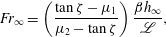 $$\begin{eqnarray}\displaystyle Fr_{\infty }=\left(\frac{\tan \unicode[STIX]{x1D701}-\unicode[STIX]{x1D707}_{1}}{\unicode[STIX]{x1D707}_{2}-\tan \unicode[STIX]{x1D701}}\right)\frac{\unicode[STIX]{x1D6FD}h_{\infty }}{\mathscr{L}}, & & \displaystyle\end{eqnarray}$$
which, by using its definition (3.4), allows the velocity
 $\bar{u}_{\infty }$
to be calculated as a function of
$\bar{u}_{\infty }$
to be calculated as a function of
 $h_{\infty }$
. Integrating the transformed mass balance (5.1), but evaluating the constant of integration at the critical point rather than in the static layer, implies that
$h_{\infty }$
. Integrating the transformed mass balance (5.1), but evaluating the constant of integration at the critical point rather than in the static layer, implies that
 $$\begin{eqnarray}\displaystyle h_{\infty }(\bar{u}_{\infty }-u_{w})=h_{c}(\bar{u}_{c}-u_{w}). & & \displaystyle\end{eqnarray}$$
Solving (5.16) and (5.17) determines the thickness far downstream for a given critical thickness
 $h_{c}$
, since
$h_{c}$
, since
 $u_{w}$
and
$u_{w}$
and
 $\bar{u}_{c}$
are known from (5.14) and (5.11), respectively.
$\bar{u}_{c}$
are known from (5.14) and (5.11), respectively.
The solutions can also be visualised in
 $(Fr,h)$
-space as shown in figure 9. The solutions connect the static layer to the steady uniform flow solution far downslope with a trajectory that smoothly passes through the critical point
$(Fr,h)$
-space as shown in figure 9. The solutions connect the static layer to the steady uniform flow solution far downslope with a trajectory that smoothly passes through the critical point
 $(Fr_{c},h_{c})$
on the
$(Fr_{c},h_{c})$
on the
 $S=0$
contour in the intermediate friction regime.
$S=0$
contour in the intermediate friction regime.
5.2 Existence of retrogressive travelling wave solutions
The retrogressive wave solutions outlined in § 5.1 exist over a range of slope angles
 $\unicode[STIX]{x1D701}$
and initial layer thicknesses
$\unicode[STIX]{x1D701}$
and initial layer thicknesses
 $h_{0}$
. An upper bound for the initial layer thickness is provided by the requirement that the static layer does not fail spontaneously, which implies that
$h_{0}$
. An upper bound for the initial layer thickness is provided by the requirement that the static layer does not fail spontaneously, which implies that
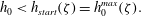 $$\begin{eqnarray}\displaystyle h_{0}<h_{start}(\unicode[STIX]{x1D701})=h_{0}^{max}(\unicode[STIX]{x1D701}). & & \displaystyle\end{eqnarray}$$
The function
 $h_{start}(\unicode[STIX]{x1D701})$
takes a finite value when
$h_{start}(\unicode[STIX]{x1D701})$
takes a finite value when
 $\unicode[STIX]{x1D701}>\unicode[STIX]{x1D701}_{3}$
as in figure 9, but is infinite for shallower inclinations
$\unicode[STIX]{x1D701}>\unicode[STIX]{x1D701}_{3}$
as in figure 9, but is infinite for shallower inclinations
 $\unicode[STIX]{x1D701}\leqslant \unicode[STIX]{x1D701}_{3}$
, in which case the initial static layer may be arbitrarily thick. A lower bound for the initial thickness
$\unicode[STIX]{x1D701}\leqslant \unicode[STIX]{x1D701}_{3}$
, in which case the initial static layer may be arbitrarily thick. A lower bound for the initial thickness
 $h_{0}$
stems from the requirement that a steady uniform flow exists far downstream, which implies that
$h_{0}$
stems from the requirement that a steady uniform flow exists far downstream, which implies that
 $h_{\infty }\geqslant h_{\ast }$
as shown in figures 9 and 10. It follows that the minimum initial thickness
$h_{\infty }\geqslant h_{\ast }$
as shown in figures 9 and 10. It follows that the minimum initial thickness
 $h_{0}$
for which a solution exists occurs when
$h_{0}$
for which a solution exists occurs when
 $h_{c}=h_{\ast }=h_{\infty }$
and
$h_{c}=h_{\ast }=h_{\infty }$
and
 $Fr=\unicode[STIX]{x1D6FD}_{\ast }$
, which, using (5.15) and (3.12), implies that
$Fr=\unicode[STIX]{x1D6FD}_{\ast }$
, which, using (5.15) and (3.12), implies that
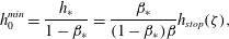 $$\begin{eqnarray}\displaystyle h_{0}^{min}=\frac{h_{\ast }}{1-\unicode[STIX]{x1D6FD}_{\ast }}=\frac{\unicode[STIX]{x1D6FD}_{\ast }}{(1-\unicode[STIX]{x1D6FD}_{\ast })\unicode[STIX]{x1D6FD}}h_{stop}(\unicode[STIX]{x1D701}), & & \displaystyle\end{eqnarray}$$
which is a constant multiple of
 $h_{stop}(\unicode[STIX]{x1D701})$
. The upper and lower bounds (5.18) and (5.19) define a region in phase space, shown in figure 11, where retrogressive waves exist. Experiments recording the existence or not of a retrogressive wave over a range of
$h_{stop}(\unicode[STIX]{x1D701})$
. The upper and lower bounds (5.18) and (5.19) define a region in phase space, shown in figure 11, where retrogressive waves exist. Experiments recording the existence or not of a retrogressive wave over a range of
 $\unicode[STIX]{x1D701}$
and
$\unicode[STIX]{x1D701}$
and
 $h_{0}$
are in good agreement with the theoretical predictions (figure 11). Below
$h_{0}$
are in good agreement with the theoretical predictions (figure 11). Below
 $h_{0}^{min}(\unicode[STIX]{x1D701})$
retrogressive failures are not observed, but avalanches can propagate downslope and in some cases, for initial layer thicknesses slightly greater than
$h_{0}^{min}(\unicode[STIX]{x1D701})$
retrogressive failures are not observed, but avalanches can propagate downslope and in some cases, for initial layer thicknesses slightly greater than
 $h_{0}^{min}(\unicode[STIX]{x1D701})$
, erosion–deposition waves (Edwards & Gray Reference Edwards and Gray2015) can form downstream of the retrogressive failure. This experimental determination of
$h_{0}^{min}(\unicode[STIX]{x1D701})$
, erosion–deposition waves (Edwards & Gray Reference Edwards and Gray2015) can form downstream of the retrogressive failure. This experimental determination of
 $h_{0}^{min}(\unicode[STIX]{x1D701})$
supports a constant value of
$h_{0}^{min}(\unicode[STIX]{x1D701})$
supports a constant value of
 $\unicode[STIX]{x1D6FD}_{\ast }$
for all inclinations (as suggested by Edwards et al.
Reference Edwards, Russell, Johnson and Gray2019) with
$\unicode[STIX]{x1D6FD}_{\ast }$
for all inclinations (as suggested by Edwards et al.
Reference Edwards, Russell, Johnson and Gray2019) with
 $\unicode[STIX]{x1D6FD}_{\ast }=0.19\approx 1.33\unicode[STIX]{x1D6FD}$
, corresponding to a minimum thickness of steady uniform flow
$\unicode[STIX]{x1D6FD}_{\ast }=0.19\approx 1.33\unicode[STIX]{x1D6FD}$
, corresponding to a minimum thickness of steady uniform flow
 $h_{\ast }\approx 1.33h_{stop}$
. The prediction for
$h_{\ast }\approx 1.33h_{stop}$
. The prediction for
 $h_{0}^{min}$
with
$h_{0}^{min}$
with
 $\unicode[STIX]{x1D6FD}_{\ast }=\unicode[STIX]{x1D6FD}$
(dotted line in figure 11, as suggested by Pouliquen & Forterre Reference Pouliquen and Forterre2002) is not in such good agreement with our experiments. The experimental phase boundary
$\unicode[STIX]{x1D6FD}_{\ast }=\unicode[STIX]{x1D6FD}$
(dotted line in figure 11, as suggested by Pouliquen & Forterre Reference Pouliquen and Forterre2002) is not in such good agreement with our experiments. The experimental phase boundary
 $h_{0}^{min}(\unicode[STIX]{x1D701})$
therefore provides an important constraint on the theory that also helps to determine
$h_{0}^{min}(\unicode[STIX]{x1D701})$
therefore provides an important constraint on the theory that also helps to determine
 $\unicode[STIX]{x1D6FD}_{\ast }$
.
$\unicode[STIX]{x1D6FD}_{\ast }$
.
Experimental phase diagram showing the values of slope angle
 $\unicode[STIX]{x1D701}$
and static layer thickness
$\unicode[STIX]{x1D701}$
and static layer thickness
 $h_{0}$
for which retrogressive failures are observed (black circles) and are not observed (crosses). This agrees well with the predicted domain of existence for
$h_{0}$
for which retrogressive failures are observed (black circles) and are not observed (crosses). This agrees well with the predicted domain of existence for
 $h_{0}\in [h_{0}^{\text{min}}(\unicode[STIX]{x1D701}),h_{start}(\unicode[STIX]{x1D701}))$
, which is shaded blue. In particular, the lower boundary
$h_{0}\in [h_{0}^{\text{min}}(\unicode[STIX]{x1D701}),h_{start}(\unicode[STIX]{x1D701}))$
, which is shaded blue. In particular, the lower boundary
 $h_{0}^{min}(\unicode[STIX]{x1D701})$
(solid black curve) is in much better agreement than when
$h_{0}^{min}(\unicode[STIX]{x1D701})$
(solid black curve) is in much better agreement than when
 $\unicode[STIX]{x1D6FD}_{\ast }=\unicode[STIX]{x1D6FD}$
(dotted curve), which corresponds to Pouliquen & Forterre’s (Reference Pouliquen and Forterre2002) original friction law. The red line represents
$\unicode[STIX]{x1D6FD}_{\ast }=\unicode[STIX]{x1D6FD}$
(dotted curve), which corresponds to Pouliquen & Forterre’s (Reference Pouliquen and Forterre2002) original friction law. The red line represents
 $h_{stop}(\unicode[STIX]{x1D701})$
, the green line to
$h_{stop}(\unicode[STIX]{x1D701})$
, the green line to
 $h_{start}(\unicode[STIX]{x1D701})$
and the vertical dashed lines correspond to the angles
$h_{start}(\unicode[STIX]{x1D701})$
and the vertical dashed lines correspond to the angles
 $\unicode[STIX]{x1D701}_{1}$
,
$\unicode[STIX]{x1D701}_{1}$
,
 $\unicode[STIX]{x1D701}_{2}$
and
$\unicode[STIX]{x1D701}_{2}$
and
 $\unicode[STIX]{x1D701}_{3}$
.
$\unicode[STIX]{x1D701}_{3}$
.
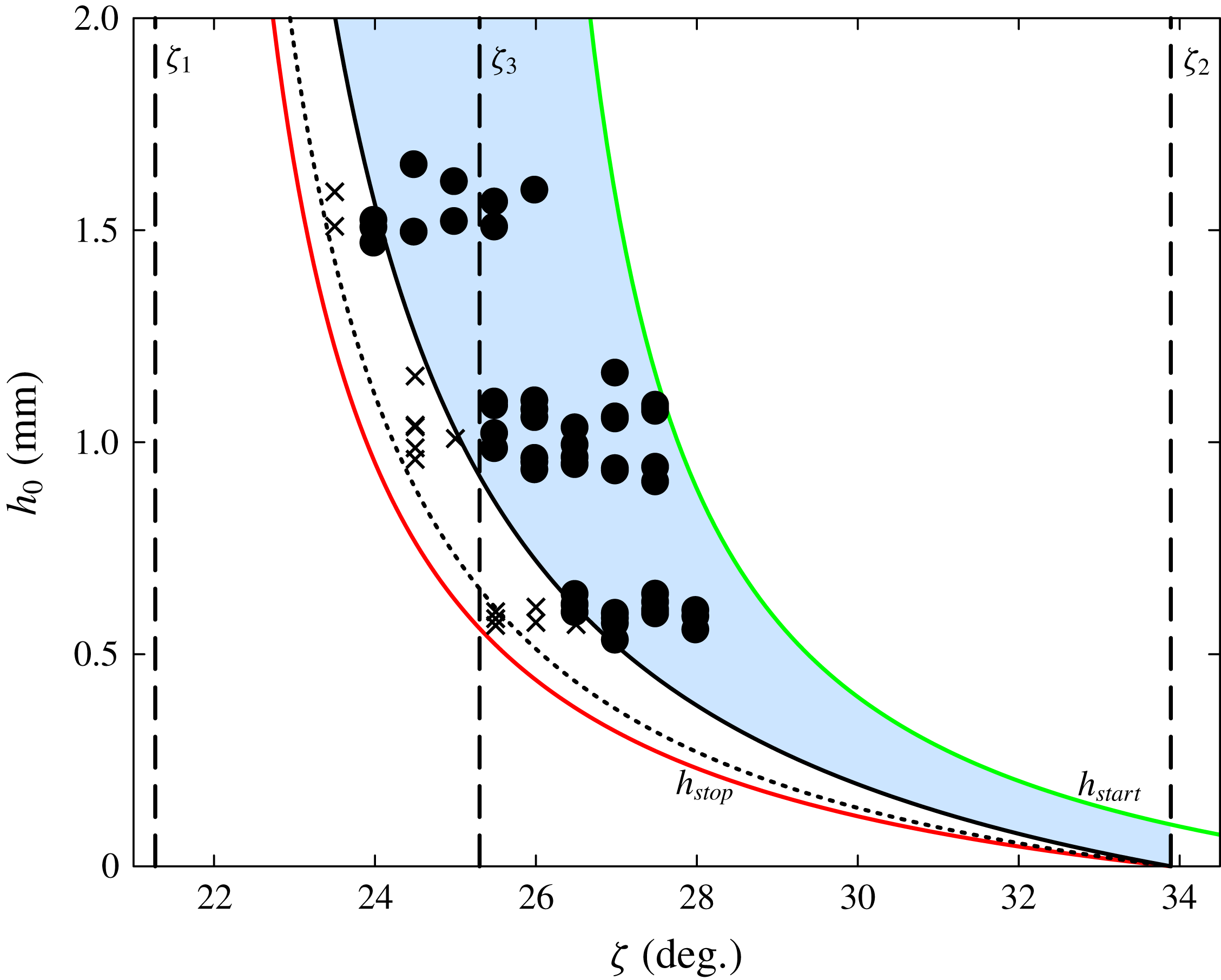
Retrogressive waves are predicted for angles up to
 $\unicode[STIX]{x1D701}_{4}=\tan ^{-1}(\unicode[STIX]{x1D707}_{3}+\unicode[STIX]{x1D707}_{2}-\unicode[STIX]{x1D707}_{1})$
, the angle at which
$\unicode[STIX]{x1D701}_{4}=\tan ^{-1}(\unicode[STIX]{x1D707}_{3}+\unicode[STIX]{x1D707}_{2}-\unicode[STIX]{x1D707}_{1})$
, the angle at which
 $h_{start}$
reaches zero. For
$h_{start}$
reaches zero. For
 $\unicode[STIX]{x1D701}>\unicode[STIX]{x1D701}_{2}$
, the method to determine the critical point and the retrogressive wave speed remains unchanged, but the flow accelerates and thins indefinitely downslope once it has failed. This regime is not observed in our experiments, because the predicted static layer depths are too small (
$\unicode[STIX]{x1D701}>\unicode[STIX]{x1D701}_{2}$
, the method to determine the critical point and the retrogressive wave speed remains unchanged, but the flow accelerates and thins indefinitely downslope once it has failed. This regime is not observed in our experiments, because the predicted static layer depths are too small (
 ${\sim}1$
grain diameter), but such solutions may be observable in grains with a larger static friction coefficient that can form thicker static layers at steep inclinations
${\sim}1$
grain diameter), but such solutions may be observable in grains with a larger static friction coefficient that can form thicker static layers at steep inclinations
 $\unicode[STIX]{x1D701}>\unicode[STIX]{x1D701}_{2}$
.
$\unicode[STIX]{x1D701}>\unicode[STIX]{x1D701}_{2}$
.
5.3 Retrogressive wave speed
The theoretical wave speed
 $|u_{w}|$
is compared with the experimentally measured values in figure 12 for a range of slope angles
$|u_{w}|$
is compared with the experimentally measured values in figure 12 for a range of slope angles
 $\unicode[STIX]{x1D701}$
and for initial layers of thickness (a)
$\unicode[STIX]{x1D701}$
and for initial layers of thickness (a)
 $h_{0}=h_{stop}(24^{\circ })=0.95$
mm and (b)
$h_{0}=h_{stop}(24^{\circ })=0.95$
mm and (b)
 $h_{0}=h_{stop}(25^{\circ })=0.63$
mm. Since both
$h_{0}=h_{stop}(25^{\circ })=0.63$
mm. Since both
 $h_{start}(\unicode[STIX]{x1D701})$
and
$h_{start}(\unicode[STIX]{x1D701})$
and
 $h_{stop}(\unicode[STIX]{x1D701})$
are monotonically decreasing functions, the upper and lower bounds (5.18) and (5.19) can be rearranged to give the maximum and minimum slope angles at which an initial layer of thickness
$h_{stop}(\unicode[STIX]{x1D701})$
are monotonically decreasing functions, the upper and lower bounds (5.18) and (5.19) can be rearranged to give the maximum and minimum slope angles at which an initial layer of thickness
 $h_{0}$
will form a retrogressive wave
$h_{0}$
will form a retrogressive wave
 $$\begin{eqnarray}\displaystyle & \displaystyle \unicode[STIX]{x1D701}^{max}=\unicode[STIX]{x1D701}_{start}(h_{0}), & \displaystyle\end{eqnarray}$$
 $$\begin{eqnarray}\displaystyle & \displaystyle \unicode[STIX]{x1D701}^{min}=\unicode[STIX]{x1D701}_{stop}\left(\frac{(1-\unicode[STIX]{x1D6FD}_{\ast })\unicode[STIX]{x1D6FD}}{\unicode[STIX]{x1D6FD}_{\ast }}h_{0}\right), & \displaystyle\end{eqnarray}$$
where
 $\unicode[STIX]{x1D701}_{stop}(h)$
and
$\unicode[STIX]{x1D701}_{stop}(h)$
and
 $\unicode[STIX]{x1D701}_{start}(h)$
are the inverse functions of
$\unicode[STIX]{x1D701}_{start}(h)$
are the inverse functions of
 $h_{stop}(\unicode[STIX]{x1D701})$
and
$h_{stop}(\unicode[STIX]{x1D701})$
and
 $h_{start}(\unicode[STIX]{x1D701})$
, respectively. For angles
$h_{start}(\unicode[STIX]{x1D701})$
, respectively. For angles
 $\unicode[STIX]{x1D701}>\unicode[STIX]{x1D701}^{max}$
the initial layer is thicker than
$\unicode[STIX]{x1D701}>\unicode[STIX]{x1D701}^{max}$
the initial layer is thicker than
 $h_{start}$
and therefore spontaneously flows off the inclined plane, while for
$h_{start}$
and therefore spontaneously flows off the inclined plane, while for
 $\unicode[STIX]{x1D701}<\unicode[STIX]{x1D701}^{min}$
a retrogressive wave does not propagate upslope, although an avalanche forms downstream of the perturbation. In both of these situations the retrogressive wave speed is defined to be zero.
$\unicode[STIX]{x1D701}<\unicode[STIX]{x1D701}^{min}$
a retrogressive wave does not propagate upslope, although an avalanche forms downstream of the perturbation. In both of these situations the retrogressive wave speed is defined to be zero.
The retrogressive wave speed
 $|u_{w}|$
for (a)
$|u_{w}|$
for (a)
 $h_{0}=h_{stop}(24^{\circ })=0.95$
mm and (b)
$h_{0}=h_{stop}(24^{\circ })=0.95$
mm and (b)
 $h_{0}=h_{stop}(25^{\circ })=0.63$
mm as a function of inclination angle
$h_{0}=h_{stop}(25^{\circ })=0.63$
mm as a function of inclination angle
 $\unicode[STIX]{x1D701}$
. The circles represent experimental data for the retrogressive front and the crosses show the cases when either (i) there is no retrogressive failure, although there is an avalanche that propagates downslope, or (ii) a static layer of thickness
$\unicode[STIX]{x1D701}$
. The circles represent experimental data for the retrogressive front and the crosses show the cases when either (i) there is no retrogressive failure, although there is an avalanche that propagates downslope, or (ii) a static layer of thickness
 $h_{0}$
can no longer be supported. The red line represents the theoretical prediction of the wave speed
$h_{0}$
can no longer be supported. The red line represents the theoretical prediction of the wave speed
 $|u_{w}|$
. The black dotted line corresponds to the prediction from Pouliquen & Forterre’s (Reference Pouliquen and Forterre2002) original friction law (5.23). Note that since
$|u_{w}|$
. The black dotted line corresponds to the prediction from Pouliquen & Forterre’s (Reference Pouliquen and Forterre2002) original friction law (5.23). Note that since
 $\unicode[STIX]{x1D6FD}_{\ast }=\unicode[STIX]{x1D6FD}$
these lines extend considerably into the region where retrogressive failures are not observed.
$\unicode[STIX]{x1D6FD}_{\ast }=\unicode[STIX]{x1D6FD}$
these lines extend considerably into the region where retrogressive failures are not observed.
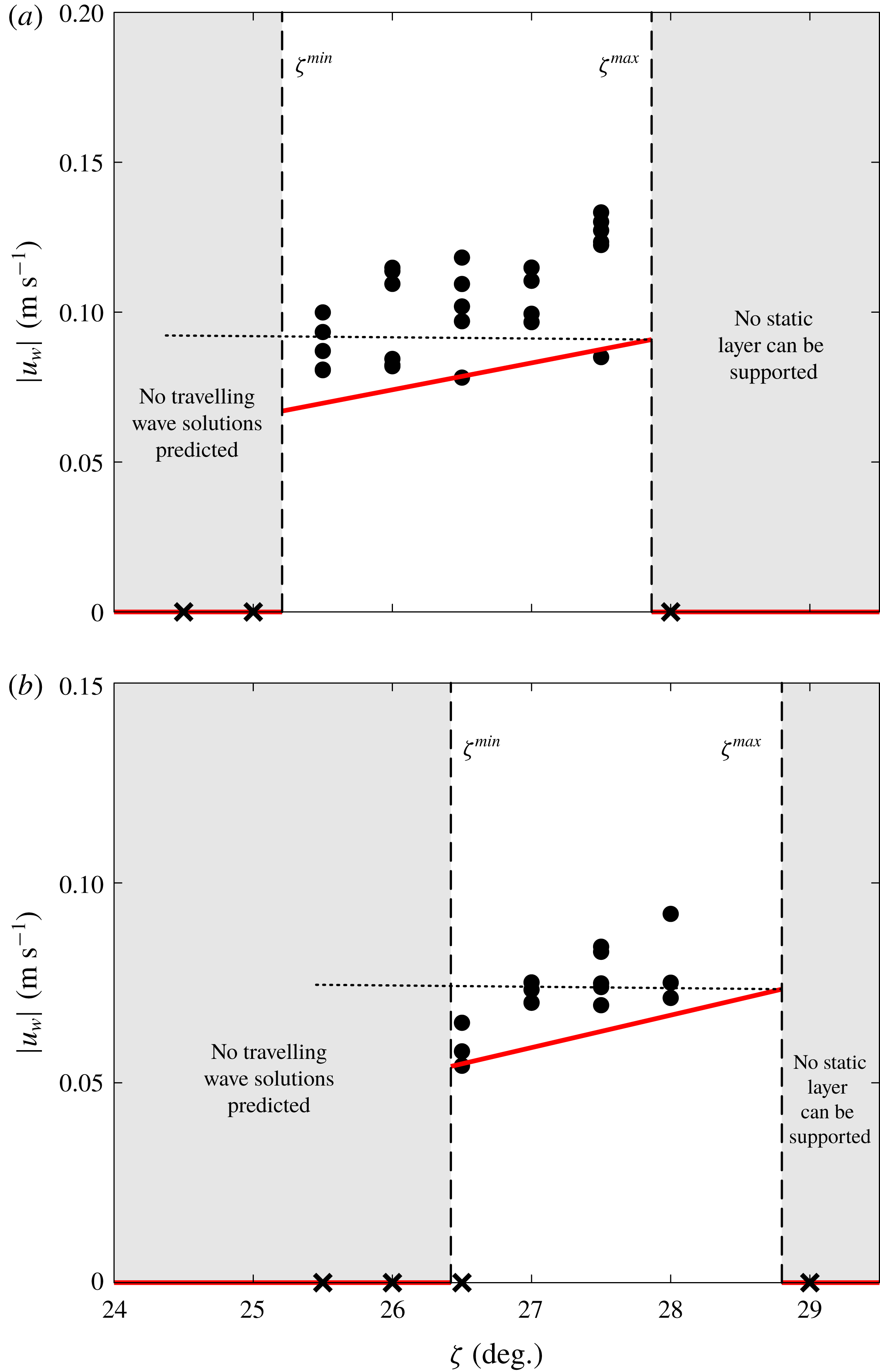
For the two sets of experiments in figure 12 the range of angles over which retrogressive failures are, and are not, observed agree well with the theoretically predicted limits
 $\unicode[STIX]{x1D701}^{min}$
and
$\unicode[STIX]{x1D701}^{min}$
and
 $\unicode[STIX]{x1D701}^{max}$
. In the range of angles where retrogressive waves are observed both sets of data show that the wave speed increases with increasing inclination angle. This trend is well predicted by the theory, but the magnitude of the wave speed is slightly under-predicted. The theory does, however, predict the immediate jump from zero up to a finite non-zero wave speed at the onset of retrogressive failures at
$\unicode[STIX]{x1D701}^{max}$
. In the range of angles where retrogressive waves are observed both sets of data show that the wave speed increases with increasing inclination angle. This trend is well predicted by the theory, but the magnitude of the wave speed is slightly under-predicted. The theory does, however, predict the immediate jump from zero up to a finite non-zero wave speed at the onset of retrogressive failures at
 $\unicode[STIX]{x1D701}=\unicode[STIX]{x1D701}^{min}$
. The scatter in the experimental data points is primarily due to the difficulty of precisely controlling the initial static layer thickness
$\unicode[STIX]{x1D701}=\unicode[STIX]{x1D701}^{min}$
. The scatter in the experimental data points is primarily due to the difficulty of precisely controlling the initial static layer thickness
 $h_{0}$
.
$h_{0}$
.
The theoretical wave velocity (5.14) is dependent on the thickness
 $h_{c}$
and the depth-averaged velocity
$h_{c}$
and the depth-averaged velocity
 $\bar{u}_{c}$
at the critical point. Substituting for
$\bar{u}_{c}$
at the critical point. Substituting for
 $\bar{u}_{c}$
from (5.11) it follows that the wave speed
$\bar{u}_{c}$
from (5.11) it follows that the wave speed
 $|u_{w}|$
can be written as
$|u_{w}|$
can be written as
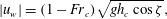 $$\begin{eqnarray}\displaystyle |u_{w}|=(1-Fr_{c})\sqrt{gh_{c}\cos \unicode[STIX]{x1D701}}, & & \displaystyle\end{eqnarray}$$
where
 $Fr_{c}(h_{c})$
is defined in (5.10). Experimental measurements of the wave speed therefore provide indirect experimental evidence for the form of the friction law in the intermediate regime
$Fr_{c}(h_{c})$
is defined in (5.10). Experimental measurements of the wave speed therefore provide indirect experimental evidence for the form of the friction law in the intermediate regime
 $0<Fr<\unicode[STIX]{x1D6FD}_{\ast }$
. This evidence is valuable because steady uniform flows, which are widely used to determine the flow rule for
$0<Fr<\unicode[STIX]{x1D6FD}_{\ast }$
. This evidence is valuable because steady uniform flows, which are widely used to determine the flow rule for
 $Fr>\unicode[STIX]{x1D6FD}_{\ast }$
(Pouliquen Reference Pouliquen1999a
), are unstable in intermediate regime
$Fr>\unicode[STIX]{x1D6FD}_{\ast }$
(Pouliquen Reference Pouliquen1999a
), are unstable in intermediate regime
 $0<Fr<\unicode[STIX]{x1D6FD}_{\ast }$
and so cannot be observed experimentally. The friction in the intermediate regime (3.7) is a power-law interpolation between the maximum static friction at
$0<Fr<\unicode[STIX]{x1D6FD}_{\ast }$
and so cannot be observed experimentally. The friction in the intermediate regime (3.7) is a power-law interpolation between the maximum static friction at
 $Fr=0$
and the minimum dynamic friction at
$Fr=0$
and the minimum dynamic friction at
 $Fr=\unicode[STIX]{x1D6FD}_{\ast }$
, with exponent
$Fr=\unicode[STIX]{x1D6FD}_{\ast }$
, with exponent
 $\unicode[STIX]{x1D705}$
that is taken to be unity (figure 13
a, inset). This form of the friction coefficient results in the retrogressive wave speed being an increasing function of the slope angle for a given layer thickness
$\unicode[STIX]{x1D705}$
that is taken to be unity (figure 13
a, inset). This form of the friction coefficient results in the retrogressive wave speed being an increasing function of the slope angle for a given layer thickness
 $h_{0}$
(figure 13
a), which is in agreement with experimental cases shown in figure 12(a,b).
$h_{0}$
(figure 13
a), which is in agreement with experimental cases shown in figure 12(a,b).
Contours of the retrogressive wave speed
 $|u_{w}|$
computed from (5.14) (black and grey solid lines), plotted with respect to the slope angle
$|u_{w}|$
computed from (5.14) (black and grey solid lines), plotted with respect to the slope angle
 $\unicode[STIX]{x1D701}$
and the initial layer thickness
$\unicode[STIX]{x1D701}$
and the initial layer thickness
 $h_{0}$
. Solutions exist for
$h_{0}$
. Solutions exist for
 $h_{0}$
between
$h_{0}$
between
 $h_{0}=h_{0}^{min}(\unicode[STIX]{x1D701})$
(black dotted line) and
$h_{0}=h_{0}^{min}(\unicode[STIX]{x1D701})$
(black dotted line) and
 $h_{0}=h_{0}^{max}(\unicode[STIX]{x1D701})$
(green line). The inset shows the friction coefficient
$h_{0}=h_{0}^{max}(\unicode[STIX]{x1D701})$
(green line). The inset shows the friction coefficient
 $\unicode[STIX]{x1D707}$
as a function of Froude number for
$\unicode[STIX]{x1D707}$
as a function of Froude number for
 $h=1$
mm. In (a) linear interpolation of the friction is used in the intermediate regime (
$h=1$
mm. In (a) linear interpolation of the friction is used in the intermediate regime (
 $\unicode[STIX]{x1D705}=1$
), leading to the experimentally observed increase in
$\unicode[STIX]{x1D705}=1$
), leading to the experimentally observed increase in
 $|u_{w}|$
with increasing
$|u_{w}|$
with increasing
 $\unicode[STIX]{x1D701}$
. In (b) a nonlinear interpolation is used (
$\unicode[STIX]{x1D701}$
. In (b) a nonlinear interpolation is used (
 $\unicode[STIX]{x1D705}=10^{-3}$
, as suggested by Pouliquen & Forterre Reference Pouliquen and Forterre2002), leading to the opposite relationship between
$\unicode[STIX]{x1D705}=10^{-3}$
, as suggested by Pouliquen & Forterre Reference Pouliquen and Forterre2002), leading to the opposite relationship between
 $|u_{w}|$
and
$|u_{w}|$
and
 $\unicode[STIX]{x1D701}$
. Note that in both of these plots the value of
$\unicode[STIX]{x1D701}$
. Note that in both of these plots the value of
 $\unicode[STIX]{x1D6FD}_{\ast }$
in table 1 is used.
$\unicode[STIX]{x1D6FD}_{\ast }$
in table 1 is used.
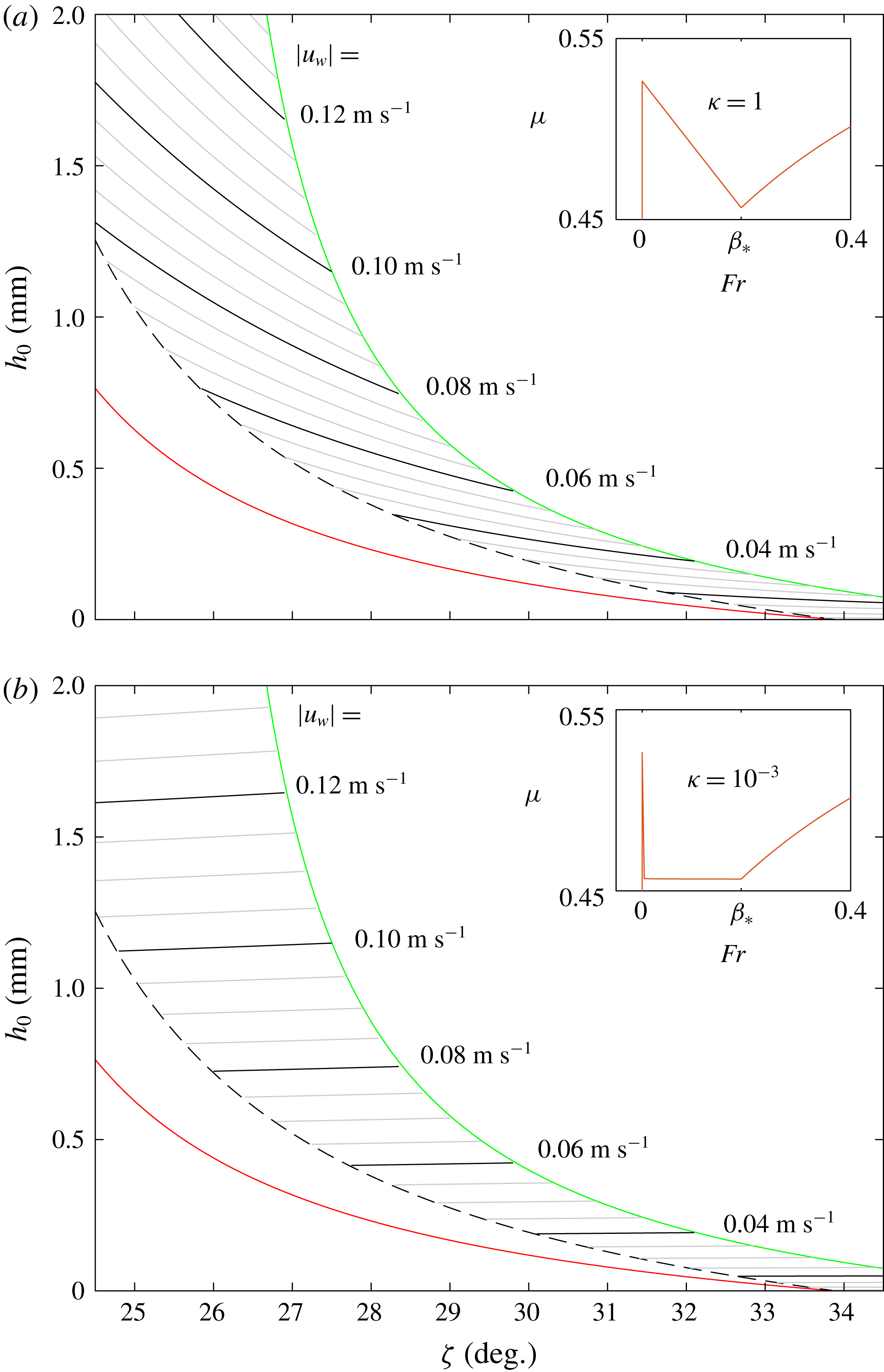
In Pouliquen & Forterre’s (Reference Pouliquen and Forterre2002) original friction law the interpolation parameter was chosen to be very small (e.g.
 $\unicode[STIX]{x1D705}=10^{-3}$
), which corresponds to a rapid decrease from the maximum static friction at low Froude numbers, as shown in the inset in figure 13(b). This choice of interpolation leads to an extremely small critical Froude number
$\unicode[STIX]{x1D705}=10^{-3}$
), which corresponds to a rapid decrease from the maximum static friction at low Froude numbers, as shown in the inset in figure 13(b). This choice of interpolation leads to an extremely small critical Froude number
 $Fr_{c}$
, and consequently
$Fr_{c}$
, and consequently
 $h_{c}\approx h_{0}$
. It follows from (5.22) that the wave speed
$h_{c}\approx h_{0}$
. It follows from (5.22) that the wave speed
 $$\begin{eqnarray}\displaystyle |u_{w}|\approx \sqrt{gh_{0}\cos \unicode[STIX]{x1D701}}. & & \displaystyle\end{eqnarray}$$
This is a slightly decreasing function of the inclination angle
 $\unicode[STIX]{x1D701}$
(see the dotted lines in figure 12 as well as figure 13
b), which is the opposite trend to that observed in the experiments in figure 12. While the scatter in experimental data make it difficult to infer the precise functional form of the friction coefficient in the intermediate regime, the clear increase in
$\unicode[STIX]{x1D701}$
(see the dotted lines in figure 12 as well as figure 13
b), which is the opposite trend to that observed in the experiments in figure 12. While the scatter in experimental data make it difficult to infer the precise functional form of the friction coefficient in the intermediate regime, the clear increase in
 $|u_{w}|$
observed with increasing
$|u_{w}|$
observed with increasing
 $\unicode[STIX]{x1D701}$
is strong evidence that the transition to the static failure criterion at
$\unicode[STIX]{x1D701}$
is strong evidence that the transition to the static failure criterion at
 $Fr=0$
is less rapid than that suggested by Pouliquen & Forterre (Reference Pouliquen and Forterre2002). Note that the solution for the original friction law of Pouliquen & Forterre (Reference Pouliquen and Forterre2002) in figure 12, with
$Fr=0$
is less rapid than that suggested by Pouliquen & Forterre (Reference Pouliquen and Forterre2002). Note that the solution for the original friction law of Pouliquen & Forterre (Reference Pouliquen and Forterre2002) in figure 12, with
 $\unicode[STIX]{x1D6FD}_{\ast }=\unicode[STIX]{x1D6FD}$
, has a much wider region in which retrogressive failures form than observed in experiments.
$\unicode[STIX]{x1D6FD}_{\ast }=\unicode[STIX]{x1D6FD}$
, has a much wider region in which retrogressive failures form than observed in experiments.
When
 $\unicode[STIX]{x1D705}=1$
the retrogressive wave speed (5.22) is an increasing function of the initial layer thickness
$\unicode[STIX]{x1D705}=1$
the retrogressive wave speed (5.22) is an increasing function of the initial layer thickness
 $h_{0}$
. For a given slope angle
$h_{0}$
. For a given slope angle
 $\unicode[STIX]{x1D701}$
, the fastest and slowest retrogressive waves therefore occur at the boundaries
$\unicode[STIX]{x1D701}$
, the fastest and slowest retrogressive waves therefore occur at the boundaries
 $h_{0}=h_{0}^{max}$
and
$h_{0}=h_{0}^{max}$
and
 $h_{0}=h_{0}^{min}$
defined in (5.18) and (5.19), respectively. For the thickest initial static layer
$h_{0}=h_{0}^{min}$
defined in (5.18) and (5.19), respectively. For the thickest initial static layer
 $h_{0}=h_{0}^{max}$
the critical point
$h_{0}=h_{0}^{max}$
the critical point
 $h_{c}$
takes its maximum value of
$h_{c}$
takes its maximum value of
 $h_{start}$
and the velocity
$h_{start}$
and the velocity
 $\bar{u}_{c}$
is zero, as shown in figure 9. It follows, from (5.14) that the maximum upslope-propagating wave speed is
$\bar{u}_{c}$
is zero, as shown in figure 9. It follows, from (5.14) that the maximum upslope-propagating wave speed is
 $$\begin{eqnarray}\displaystyle |u_{w}|=|u_{w}|^{max}=\sqrt{gh_{start}\cos \unicode[STIX]{x1D701}}. & & \displaystyle\end{eqnarray}$$
Conversely, when
 $h_{0}=h_{0}^{min}$
, the critical thickness
$h_{0}=h_{0}^{min}$
, the critical thickness
 $h_{c}$
takes its minimum value of
$h_{c}$
takes its minimum value of
 $h_{\ast }$
and the Froude number
$h_{\ast }$
and the Froude number
 $Fr_{c}$
takes its maximum value of
$Fr_{c}$
takes its maximum value of
 $\unicode[STIX]{x1D6FD}_{\ast }$
as shown in figure 9. This produces the slowest retrogressive wave speed for a given thickness
$\unicode[STIX]{x1D6FD}_{\ast }$
as shown in figure 9. This produces the slowest retrogressive wave speed for a given thickness
 $h_{0}$
, which using (3.12) and (5.22), is
$h_{0}$
, which using (3.12) and (5.22), is
 $$\begin{eqnarray}\displaystyle |u_{w}|=|u_{w}|^{min}=(1-\unicode[STIX]{x1D6FD}_{\ast })\sqrt{gh_{\ast }\cos \unicode[STIX]{x1D701}}=(1-\unicode[STIX]{x1D6FD}_{\ast })\sqrt{(\unicode[STIX]{x1D6FD}_{\ast }/\unicode[STIX]{x1D6FD})gh_{stop}\cos \unicode[STIX]{x1D701}}. & & \displaystyle\end{eqnarray}$$
This is also the wave speed at the onset of retrogressive failure at
 $\unicode[STIX]{x1D701}=\unicode[STIX]{x1D701}^{min}$
.
$\unicode[STIX]{x1D701}=\unicode[STIX]{x1D701}^{min}$
.
6 Conclusions and discussion
Frictional hysteresis (Daerr & Douady Reference Daerr and Douady1999; Daerr Reference Daerr2001; Aranson & Tsimring Reference Aranson and Tsimring2002; Pouliquen & Forterre Reference Pouliquen and Forterre2002; Edwards et al. Reference Edwards, Viroulet, Kokelaar and Gray2017, Reference Edwards, Russell, Johnson and Gray2019) results in a range of thicknesses over which both static and moving layers of material can coexist in a granular flow. This property is fundamental to the retrogressive failures studied here, which combine a thicker static and thinner flowing layer. In more complex three-dimensional flows, hysteresis gives rise to a wide range of subtle morphological features on erodible beds, such as incised troughs (Daerr & Douady Reference Daerr and Douady1999; Edwards et al. Reference Edwards, Viroulet, Kokelaar and Gray2017), super-elevated channels and static levees (Edwards et al. Reference Edwards, Viroulet, Kokelaar and Gray2017). It also plays a crucial role in the selection of the height and width of self-channelised flows on non-erodible beds (Rocha et al. Reference Rocha, Johnson and Gray2019), which can significantly extend the run-out distance of hazardous geophysical mass flows (Félix & Thomas Reference Félix and Thomas2004; Mangeney et al. Reference Mangeney, Bouchut, Thomas, Vilotte and Bristeau2007; Johnson et al. Reference Johnson, Kokelaar, Iverson, Logan, LaHusen and Gray2012; Kokelaar et al. Reference Kokelaar, Graham, Gray and Vallance2014).
In this paper, it is shown experimentally that a static layer of thickness
 $h_{0}=h_{stop}(\unicode[STIX]{x1D701}_{0})$
on a chute inclined at angle
$h_{0}=h_{stop}(\unicode[STIX]{x1D701}_{0})$
on a chute inclined at angle
 $\unicode[STIX]{x1D701}\in (\unicode[STIX]{x1D701}_{0},\unicode[STIX]{x1D701}_{start})$
can be eroded by a planar retrogressive failure, which separates static and flowing material and propagates upslope at constant speed (figures 1–5). These planar retrogressive failures occur when the deposit is perturbed along a straight line across the slope rather than just at a single point, as in the experiments of Daerr & Douady (Reference Daerr and Douady1999). The spatial uniformity in the cross-slope
$\unicode[STIX]{x1D701}\in (\unicode[STIX]{x1D701}_{0},\unicode[STIX]{x1D701}_{start})$
can be eroded by a planar retrogressive failure, which separates static and flowing material and propagates upslope at constant speed (figures 1–5). These planar retrogressive failures occur when the deposit is perturbed along a straight line across the slope rather than just at a single point, as in the experiments of Daerr & Douady (Reference Daerr and Douady1999). The spatial uniformity in the cross-slope
 $y$
direction allows the whole process to be modelled with a relatively simple one-dimensional depth-averaged avalanche model that uses the non-monotonic effective basal friction law of Edwards et al. (Reference Edwards, Viroulet, Kokelaar and Gray2017, Reference Edwards, Russell, Johnson and Gray2019).
$y$
direction allows the whole process to be modelled with a relatively simple one-dimensional depth-averaged avalanche model that uses the non-monotonic effective basal friction law of Edwards et al. (Reference Edwards, Viroulet, Kokelaar and Gray2017, Reference Edwards, Russell, Johnson and Gray2019).
Both direct numerical simulations (figures 7–8) and the experimental space–time plot (figure 4) suggest that the retrogressive failure rapidly develops into a travelling wave. In § 5 the travelling wave ansatz is used to derive exact solutions for the speed of the wave
 $u_{w}$
and the associated initial deposit height
$u_{w}$
and the associated initial deposit height
 $h_{0}$
, which are dependent on a critical point where the flow has thickness
$h_{0}$
, which are dependent on a critical point where the flow has thickness
 $h_{c}$
. This critical thickness is determined by the requirements that (i) it is a steady uniform flow solution (5.10) to the depth-averaged momentum balance (3.2) with the intermediate friction law (3.7) and (ii) the wave speed is equal to that of the upward hyperbolic characteristic. As a result, at the critical point, both the numerator and the denominator of the ODE (5.5) are zero and hence solutions exist that smoothly pass through
$h_{c}$
. This critical thickness is determined by the requirements that (i) it is a steady uniform flow solution (5.10) to the depth-averaged momentum balance (3.2) with the intermediate friction law (3.7) and (ii) the wave speed is equal to that of the upward hyperbolic characteristic. As a result, at the critical point, both the numerator and the denominator of the ODE (5.5) are zero and hence solutions exist that smoothly pass through
 $h=h_{c}$
with a finite gradient, connecting the static and flowing layers upstream and downstream of the wave.
$h=h_{c}$
with a finite gradient, connecting the static and flowing layers upstream and downstream of the wave.
The exact travelling wave solution accurately predicts the range of slope angles
 $\unicode[STIX]{x1D701}$
and initial layer thicknesses
$\unicode[STIX]{x1D701}$
and initial layer thicknesses
 $h_{0}$
for which retrogressive waves exist. The lower phase boundary, separating upslope propagating retrogressive failures from failures that only propagate downslope, is a sensitive test of the thinnest possible steady uniform flow. Figure 11 shows that this boundary is in excellent agreement with the experimentally determined phase boundary and is therefore supportive of Edwards et al.’s (Reference Edwards, Russell, Johnson and Gray2019) idea that the transition between intermediate and dynamic regimes occurs at constant Froude number
$h_{0}$
for which retrogressive waves exist. The lower phase boundary, separating upslope propagating retrogressive failures from failures that only propagate downslope, is a sensitive test of the thinnest possible steady uniform flow. Figure 11 shows that this boundary is in excellent agreement with the experimentally determined phase boundary and is therefore supportive of Edwards et al.’s (Reference Edwards, Russell, Johnson and Gray2019) idea that the transition between intermediate and dynamic regimes occurs at constant Froude number
 $Fr=\unicode[STIX]{x1D6FD}_{\ast }>\unicode[STIX]{x1D6FD}$
, rather than at
$Fr=\unicode[STIX]{x1D6FD}_{\ast }>\unicode[STIX]{x1D6FD}$
, rather than at
 $Fr=\unicode[STIX]{x1D6FD}$
(Pouliquen & Forterre Reference Pouliquen and Forterre2002). At this onset of retrogressive failure, a jump to a finite non-zero wave speed is correctly predicted by the model (figure 12), which is a prediction that has previously been obtained only through the introduction of an additional order parameter and associated governing equation (Aranson & Tsimring Reference Aranson and Tsimring2001, Reference Aranson and Tsimring2002).
$Fr=\unicode[STIX]{x1D6FD}$
(Pouliquen & Forterre Reference Pouliquen and Forterre2002). At this onset of retrogressive failure, a jump to a finite non-zero wave speed is correctly predicted by the model (figure 12), which is a prediction that has previously been obtained only through the introduction of an additional order parameter and associated governing equation (Aranson & Tsimring Reference Aranson and Tsimring2001, Reference Aranson and Tsimring2002).
The wave speed (5.14) is dependent on the velocity and thickness at the critical point, which lies in the intermediate friction regime as shown in figure 9. Since steady uniform flows in this regime are inherently unstable and so are not observable experimentally, the retrogressive wave therefore provides a very important means of probing the functional form of the friction law in this region. The model captures the experimental trend that, for a fixed value of the initial layer
 $h_{0}$
, waves move upslope faster at higher inclinations (figure 12). In contrast, the highly nonlinear interpolation suggested by Pouliquen & Forterre (Reference Pouliquen and Forterre2002) predicts a slight decrease in the wave speed with increasing inclination angle, which is the opposite trend to that observed in the experiments. Our results therefore provide new evidence that the friction coefficient varies appreciably through the whole range
$h_{0}$
, waves move upslope faster at higher inclinations (figure 12). In contrast, the highly nonlinear interpolation suggested by Pouliquen & Forterre (Reference Pouliquen and Forterre2002) predicts a slight decrease in the wave speed with increasing inclination angle, which is the opposite trend to that observed in the experiments. Our results therefore provide new evidence that the friction coefficient varies appreciably through the whole range
 $0<Fr<\unicode[STIX]{x1D6FD}_{\ast }$
and that a linear interpolation with
$0<Fr<\unicode[STIX]{x1D6FD}_{\ast }$
and that a linear interpolation with
 $\unicode[STIX]{x1D705}=1$
is a more accurate parametrisation than using the value of
$\unicode[STIX]{x1D705}=1$
is a more accurate parametrisation than using the value of
 $\unicode[STIX]{x1D705}=10^{-3}$
of Pouliquen & Forterre (Reference Pouliquen and Forterre2002).
$\unicode[STIX]{x1D705}=10^{-3}$
of Pouliquen & Forterre (Reference Pouliquen and Forterre2002).
The experiments and modelling of this paper indicate that for thin flows the apparent basal friction rises appreciably when the Froude number decreases below
 $\unicode[STIX]{x1D6FD}_{\ast }=0.19$
. This suggests that the higher friction associated with static grains may play a role in more rapid flows (up to
$\unicode[STIX]{x1D6FD}_{\ast }=0.19$
. This suggests that the higher friction associated with static grains may play a role in more rapid flows (up to
 $Fr\approx 0.19$
) than has been suggested previously (Pouliquen & Forterre Reference Pouliquen and Forterre2002). A possible mechanism for this is that the failure of grains occurs through (rapid) progressive erosion, in which grains at the surface are the first to start flowing, followed by those near the bed. The increase in basal friction inferred for
$Fr\approx 0.19$
) than has been suggested previously (Pouliquen & Forterre Reference Pouliquen and Forterre2002). A possible mechanism for this is that the failure of grains occurs through (rapid) progressive erosion, in which grains at the surface are the first to start flowing, followed by those near the bed. The increase in basal friction inferred for
 $Fr<\unicode[STIX]{x1D6FD}_{\ast }$
would then be a consequence of depth integrating over a flow in which only the uppermost part is flowing. The steady-state velocity profiles predicted by discrete particle simulations and non-local rheological models of shallow flows (Silbert, Landry & Grest Reference Silbert, Landry and Grest2003; Kamrin & Henann Reference Kamrin and Henann2015) are broadly supportive of this hypothesis, with the lower part of the velocity profile of slow, shallow flows exhibiting very little shear.
$Fr<\unicode[STIX]{x1D6FD}_{\ast }$
would then be a consequence of depth integrating over a flow in which only the uppermost part is flowing. The steady-state velocity profiles predicted by discrete particle simulations and non-local rheological models of shallow flows (Silbert, Landry & Grest Reference Silbert, Landry and Grest2003; Kamrin & Henann Reference Kamrin and Henann2015) are broadly supportive of this hypothesis, with the lower part of the velocity profile of slow, shallow flows exhibiting very little shear.
The retrogressive failure wave exemplifies several physical mechanisms that have yet to be fully incorporated into non-depth-integrated models of granular rheology. The flow depends crucially on non-local rheological behaviour, not only in flowing regions where the non-locality leads to the minimum flow thickness
 $h_{\ast }$
, but also in static layers where the non-locality results in a maximum stable layer thickness
$h_{\ast }$
, but also in static layers where the non-locality results in a maximum stable layer thickness
 $h_{start}$
. Frictional hysteresis plays an equally important role, allowing these static and flowing layers to co-exist at the same slope angle. While many models of granular rheology are based on steady-state behaviour, the retrogressive wave is highly transient: the transition from static to flowing equilibrium states in the wave takes less than 100 ms. Furthermore, the critical point analysis suggests that the speed of the retrogressive wave is sensitive to this transient flow within the wave itself, not simply on the steady states either side of it. The retrogressive wave may therefore provide a stringent test case for future rheological models that aim to capture non-local, hysteretic and transient phenomena in granular flows.
$h_{start}$
. Frictional hysteresis plays an equally important role, allowing these static and flowing layers to co-exist at the same slope angle. While many models of granular rheology are based on steady-state behaviour, the retrogressive wave is highly transient: the transition from static to flowing equilibrium states in the wave takes less than 100 ms. Furthermore, the critical point analysis suggests that the speed of the retrogressive wave is sensitive to this transient flow within the wave itself, not simply on the steady states either side of it. The retrogressive wave may therefore provide a stringent test case for future rheological models that aim to capture non-local, hysteretic and transient phenomena in granular flows.
Acknowledgements
This research was supported by NERC grants NE/E003206/1 and NE/K003011/1 as well as EPSRC grants EP/I019189/1, EP/K00428X/1 and EP/M022447/1. J.M.N.T.G. is a Royal Society Wolfson Research Merit Award holder (WM150058) and an EPSRC Established Career Fellow (EP/M022447/1). F.M.R. acknowledges financial support from CNPq, Conselho Nacional de Desenvolvimento Científico e Tecnológico – Brazil. A.S.R. would like to thank C. Tregaskis and D. Tsuji for their help with performing the experiments. All research data supporting this publication are directly available within this publication.
Supplementary movies
Supplementary movies are available at https://doi.org/10.1017/jfm.2019.215.


 Open access