


1. Introduction
A number of canonical flows have laminar solutions that remain stable to small disturbances at all values of the Reynolds number (Wedin, Bottaro & Nagata Reference Wedin, Bottaro and Nagata2009). Couette flow, Hagen–Poiseuille flow or flow in narrow rectangular-duct of width-to-height aspect ratio below approximately 3.2 (Tatsumi & Yoshimura Reference Tatsumi and Yoshimura1990; Pushenko & Gepner Reference Pushenko and Gepner2021) and specifically the square-duct flow are such examples. Consequently, the laminar solution remains an attractor in its finite neighbourhood irrespective of the Reynolds number, and any non-laminar states that could emerge remain disconnected from this laminar solution. In this sense, the departure of the flow from the laminar form cannot be seen as resulting from a sequence of bifurcations taking it away from the laminar solution to wander the state space. On the contrary, the onset of non-laminar dynamics is instead related to the emergence of unstable, simple invariant solutions in the form of travelling waves or periodic or relative periodic orbits. Those simple, invariant solutions remain separated, in the linear sense, from the laminar solution and require finite-amplitude perturbations to be reached. At the same time, the unstable invariant solutions are thought to appear in the state space through saddle-node bifurcations and are often described as low-dimensional invariant sets. Such low-dimensional sets act by attracting the flow state along their stable manifold to later eject it along their unstable directions towards other such states. In this sense, those low-dimensional sets constitute the skeleton of the turbulent attractor (Hof et al. Reference Hof, van Doorne, Westerweel, Nieuwstadt, Faisst, Eckhardt, Wedin, Kerswell and Waleffe2004; Wedin et al. Reference Wedin, Bottaro and Nagata2009).
The fact that invariant states are unstable explains why the flow does not settle onto them but rather wanders the phase space, shadowing their manifolds and only approaching such states to spend substantial amounts of time in their proximity (Jimenez Reference Jimenez1987; Kawahara, Uhlmann & van Veen Reference Kawahara, Uhlmann and van Veen2012). Since invariant solutions seem to hold the apparent organising role over the turbulent dynamics, at least in the moderate Reynolds number range, identification of such solutions is a worthwhile endeavour and, in reality, has been undertaken for a range of canonical flows, such as Couette (Kawahara & Kida Reference Kawahara and Kida2001; Gibson, Halcrow & Cvitanović Reference Gibson, Halcrow and Cvitanović2009; Brand & Gibson Reference Brand and Gibson2014), Poiseuille (Ehrenstein & Koch Reference Ehrenstein and Koch1991; Zammert & Eckhardt Reference Zammert and Eckhardt2014) or circular-pipe flow (Pringle & Kerswell Reference Pringle and Kerswell2007; Avila et al. Reference Avila, Mellibovsky, Roland and Hof2013; Chantry, Willis & Kerswell Reference Chantry, Willis and Kerswell2014). For the square-duct problem, several invariant states in the form of non-localised, streamwise periodic travelling waves, thought to reproduce statistical characteristics of the turbulent duct flow (Kawahara et al. Reference Kawahara, Uhlmann and van Veen2012), have been established using homotopy (Wedin et al. Reference Wedin, Bottaro and Nagata2009; Okino et al. Reference Okino, Nagata, Wedin and Bottaro2010; Uhlmann, Kawahara & Pinelli Reference Uhlmann, Kawahara and Pinelli2010). However, Biau, Soueid & Bottaro (Reference Biau, Soueid and Bottaro2008) applied a linear transient growth (Schmid & Henningson Reference Schmid and Henningson2001) technique to establish a set of optimal (streamwise independent rolls) and sub-optimal (streamwise varying solutions) initial conditions used afterwards in the nonlinear analysis as initial perturbations. This work was extended to quasi-nonlinear optimisation by Biau & Bottaro (Reference Biau and Bottaro2009). For the case of linearly stable flows, the laminar solution remains disconnected from expected invariant solutions and the linear approximation disregards nonlinear interactions, and some interesting results have been obtained. It was illustrated that while the sub-optimal conditions are inferior for producing large amplifications under the linear assumption, at the same time, those solutions can lead to a long-lasting complicated response when evolved by the nonlinear operator. This is in contrast to the optimal initial conditions (streamwise independent rolls) that resulted in rapid laminarisation. It is also indicated that the sub-optimal initial results of Biau et al. (Reference Biau, Soueid and Bottaro2008) resemble qualitatively the solutions obtained for marginally turbulent states characterised by Uhlmann et al. (Reference Uhlmann, Pinelli, Kawahara and Sekimoto2007) and also reported by Gavrilakis (Reference Gavrilakis1992).
An interesting problem is the identification of the typical perturbation shape and amplitude that takes the flow to the edge that separates the laminar attraction basin from the turbulent one. In other words, the identification of such invariant solutions to the Navier–Stokes system that have co-dimension one stable manifold (or unstable manifold of dimension one). The stable manifold of this invariant state forms an edge separating the laminar and turbulent attraction basins in state space, while the invariant state itself behaves as a relative attractor on this boundary (Zammert & Eckhardt Reference Zammert and Eckhardt2014) and, at least locally, governs the transition process. Such invariant states are referred to as edge states and have been identified for some canonical cases, e.g. Poiseuille flow (Zammert & Eckhardt Reference Zammert and Eckhardt2014), Couette flow (Schneider, Marinc & Eckhardt Reference Schneider, Marinc and Eckhardt2010) and circular-pipe flow under conditions of symmetry (Pringle & Kerswell Reference Pringle and Kerswell2007; Duguet, Willis & Kerswell Reference Duguet, Willis and Kerswell2008; Avila et al. Reference Avila, Mellibovsky, Roland and Hof2013). Some of those exhibit spatial localisation in a large periodic domain. It seems, however, that the problem of the flow in a narrow rectangular-duct, and especially the square-duct flow remains open. While equilibrium solutions in the form of streamwise periodic travelling waves (Wedin et al. Reference Wedin, Bottaro and Nagata2009; Okino et al. Reference Okino, Nagata, Wedin and Bottaro2010; Uhlmann et al. Reference Uhlmann, Kawahara and Pinelli2010; Okino & Nagata Reference Okino and Nagata2012), some of which are also edge states in symmetric sub-space (Scherer, Uhlmann & Kawahara Reference Scherer, Uhlmann and Kawahara2024), have been found, the identification of localised invariant states in the full or even the symmetric sub-space remains a challenge, which we address in this work.
Consequently, this work aims to identify and characterise a particular invariant solution to square-duct flow that can also appear to be an edge state when a certain symmetry (i.e. $\pi$
-rotational symmetry with respect to a duct centreline) is invoked. The identified solution features significant streamwise localisation, making it the first ever reported localised solution to the square-duct flow, and has a form of a steady travelling wave that is very close to the laminar solution in the sense of the energy of the velocity perturbation and the hydraulic resistance. We start with edge tracking using a classical bisection approach (Itano & Toh Reference Itano and Toh2001; Skufca, Yorke & Eckhardt Reference Skufca, Yorke and Eckhardt2006) in the
$\pi$
-rotational symmetry with respect to a duct centreline) is invoked. The identified solution features significant streamwise localisation, making it the first ever reported localised solution to the square-duct flow, and has a form of a steady travelling wave that is very close to the laminar solution in the sense of the energy of the velocity perturbation and the hydraulic resistance. We start with edge tracking using a classical bisection approach (Itano & Toh Reference Itano and Toh2001; Skufca, Yorke & Eckhardt Reference Skufca, Yorke and Eckhardt2006) in the $\pi$
-rotationally symmetric sub-space. As a consequence of edge tracking, the mirror symmetries with respect to the wall bisectors appear autonomously in the edge state. In the later stage of edge tracking, therefore, we confine our considerations to the double mirror-symmetric sub-space, which improves overall convergence while also decreasing the computational size of the problem. The convergence process is concluded with the Newton–Krylov procedure followed by stability analysis of the obtained equilibrium state using ARPACK (Lehoucq, Sorensen & Yang Reference Lehoucq, Sorensen and Yang1998) procedures, based on the Arnoldi process in the form outlined by Viswanath (Reference Viswanath2007, Reference Viswanath2009). A performed stability analysis indicates that the identified state remains an edge state in the symmetric sub-space for a range of the Reynolds number
$\pi$
-rotationally symmetric sub-space. As a consequence of edge tracking, the mirror symmetries with respect to the wall bisectors appear autonomously in the edge state. In the later stage of edge tracking, therefore, we confine our considerations to the double mirror-symmetric sub-space, which improves overall convergence while also decreasing the computational size of the problem. The convergence process is concluded with the Newton–Krylov procedure followed by stability analysis of the obtained equilibrium state using ARPACK (Lehoucq, Sorensen & Yang Reference Lehoucq, Sorensen and Yang1998) procedures, based on the Arnoldi process in the form outlined by Viswanath (Reference Viswanath2007, Reference Viswanath2009). A performed stability analysis indicates that the identified state remains an edge state in the symmetric sub-space for a range of the Reynolds number ${Re}$
. At the same time, the full-space configuration has an additional unstable direction. We then apply a continuation method (Dijkstra et al. Reference Dijkstra2014) and track the computed invariant state in
${Re}$
. At the same time, the full-space configuration has an additional unstable direction. We then apply a continuation method (Dijkstra et al. Reference Dijkstra2014) and track the computed invariant state in ${Re}$
and approach the saddle-node bifurcation that gives rise to the determined state and also identify the upper branch (UB) that is also localised. We follow with our analysis and examine the developed turbulent duct flow and focus on some of the most prominent characteristics of the flow. Mainly, we look into the onset of either eight- or four-vortex states (Gavrilakis Reference Gavrilakis1992; Uhlmann et al. Reference Uhlmann, Pinelli, Kawahara and Sekimoto2007; Pirozzoli et al. Reference Pirozzoli, Modesti, Orlandi and Grasso2018) that result from averaging of the flow field, but can also be observed, to a degree, to transpire in instantaneous snapshots of the velocity field. Finally, we examine the ability of the flow to temporarily form velocity fields with increased symmetry. Our results indicate that this transient symmetrisation of the flow field correlates with the onset of a much more pronounced four-vortex state accompanied by streamwise localisation of the turbulence structures. This flow behaviour suggests a connection of such transient flow states to the identified invariant solution. This apparent connection makes the identified, streamwise localised solution physically relevant, suggesting that the symmetric sub-space laminar–turbulent edge passes through the full-space turbulent attractor. Consequently, the symmetric sub-space edge solution identified in this work seems to be embedded into the turbulent attractor itself.
${Re}$
and approach the saddle-node bifurcation that gives rise to the determined state and also identify the upper branch (UB) that is also localised. We follow with our analysis and examine the developed turbulent duct flow and focus on some of the most prominent characteristics of the flow. Mainly, we look into the onset of either eight- or four-vortex states (Gavrilakis Reference Gavrilakis1992; Uhlmann et al. Reference Uhlmann, Pinelli, Kawahara and Sekimoto2007; Pirozzoli et al. Reference Pirozzoli, Modesti, Orlandi and Grasso2018) that result from averaging of the flow field, but can also be observed, to a degree, to transpire in instantaneous snapshots of the velocity field. Finally, we examine the ability of the flow to temporarily form velocity fields with increased symmetry. Our results indicate that this transient symmetrisation of the flow field correlates with the onset of a much more pronounced four-vortex state accompanied by streamwise localisation of the turbulence structures. This flow behaviour suggests a connection of such transient flow states to the identified invariant solution. This apparent connection makes the identified, streamwise localised solution physically relevant, suggesting that the symmetric sub-space laminar–turbulent edge passes through the full-space turbulent attractor. Consequently, the symmetric sub-space edge solution identified in this work seems to be embedded into the turbulent attractor itself.
The techniques used in this work differ from those more commonly applied for this type of research. The main difference is in the fact that we employ a Spectral Element hp Method (SEM), as implemented in Nektar (Cantwell et al. Reference Cantwell2015), leveraging domain decomposition into elements (h) together with polynomial interpolation (p) within each element to obtain the desired discretisation resolution. This is in contrast to the global spectral Fourier–Chebyshev (Boyd Reference Boyd2001) discretisations that seem to be more commonly applied for this type of work (e.g. Biau et al. Reference Biau, Soueid and Bottaro2008; Biau & Bottaro Reference Biau and Bottaro2009; Gibson et al. Reference Gibson, Halcrow and Cvitanović2009; Uhlmann et al. Reference Uhlmann, Kawahara and Pinelli2010; Zammert & Eckhardt Reference Zammert and Eckhardt2014 and many others). In fact, to the best of the authors’ knowledge, this work marks the first time SEM is applied to the identification of invariant solutions to the Navier–Stokes system. The importance of this lies in the fact that SEM allows for applications in more complex geometrical configurations, as opposed to methods relying on global spatial discretisation. Consequently, the approach to invoking symmetries applied here is not based on the manipulation of the applied polynomial base to select modes of appropriate parity, but resorts to the imposition of appropriate boundary conditions. We enforce a mix of either rotationally ‘periodic’ or Dirichlet/Neumann boundary conditions onto velocity components at chosen symmetry planes, which would result from the symmetry we wish to impose rather than enforcing it via applied discretisation. It should be stressed that this approach does not necessarily guarantee to result in symmetry, but we have not experienced this as a problem for convergence in our approach. Consequently, the method applied here is computationally very effective in handling individual nonlinear simulations and allows to decrease the problem size whenever symmetries are used.
This paper is organised in the following way: § 2 outlines the problem and gives a brief outline of the applied numerical approach. Edge-tracking process and description of the identified travelling-wave solution are provided in § 3. Section 4 discusses properties of the turbulent state and characterises the onset of the four- and eight-vortex state, as well as the ability of the flow to temporarily form states that show increased flow symmetrisation and streamwise localisation, which seems to correspond to the identified invariant state. We conclude with a summary and main conclusions of this work in § 5.
2. Problem statement
Consider flow of an incompressible Newtonian fluid through a square-duct shown schematically in figure 1 with walls located at $x=\pm h$
and
$x=\pm h$
and $y=\pm h$
. The flow is driven by a constant-in-time pressure gradient and is assumed periodic in the streamwise
$y=\pm h$
. The flow is driven by a constant-in-time pressure gradient and is assumed periodic in the streamwise $z$
-direction with the periodicity
$z$
-direction with the periodicity $L_z=8\pi h$
, which seems to be close to the minimal streamwise length that allows for the existence of the streamwise localised solution discussed here (Okino Reference Okino2014). All geometric quantities are normalised with half of the duct width
$L_z=8\pi h$
, which seems to be close to the minimal streamwise length that allows for the existence of the streamwise localised solution discussed here (Okino Reference Okino2014). All geometric quantities are normalised with half of the duct width $h$
, and density
$h$
, and density $\rho$
is taken as a unit. Centreline velocity
$\rho$
is taken as a unit. Centreline velocity $W$
of the steady, laminar, quasi-parabolic velocity profile scales velocity and consequently,
$W$
of the steady, laminar, quasi-parabolic velocity profile scales velocity and consequently, ${Re}=W h/\nu$
gives the Reynolds number with
${Re}=W h/\nu$
gives the Reynolds number with $\nu$
being the kinematic viscosity. The flow is governed by continuity and momentum equations of the dimensionless form:
$\nu$
being the kinematic viscosity. The flow is governed by continuity and momentum equations of the dimensionless form: $ \begin{equation} \begin{cases} \boldsymbol{\nabla \cdot u} = 0, \\ \dfrac {\partial \boldsymbol {u}}{\partial t}+(\boldsymbol {u}\boldsymbol{\cdot} \boldsymbol{\nabla} )\boldsymbol {u}=-\boldsymbol{\nabla} p+\dfrac {1}{{Re}}\Delta \boldsymbol {u} + \xi \boldsymbol{\hat {z}}, \end{cases} \end{equation}$
with $\boldsymbol{u} = [u, v, w]^{\rm T}$
,
$\boldsymbol{u} = [u, v, w]^{\rm T}$
, $p$
and
$p$
and $\boldsymbol{\hat{z}}$
being the velocity vector, the pressure and a unit vector in the streamwise direction, respectively. Hereafter, only dimensionless values are used unless stated otherwise. No-slip, impermeable conditions are imposed on the duct walls and periodic condition is imposed in the streamwise direction. The laminar, steady flow reduces (2.1) to the Poisson problem for the streamwise velocity
$\boldsymbol{\hat{z}}$
being the velocity vector, the pressure and a unit vector in the streamwise direction, respectively. Hereafter, only dimensionless values are used unless stated otherwise. No-slip, impermeable conditions are imposed on the duct walls and periodic condition is imposed in the streamwise direction. The laminar, steady flow reduces (2.1) to the Poisson problem for the streamwise velocity $\Delta w = {-{Re}{\xi }}$
, where
$\Delta w = {-{Re}{\xi }}$
, where $\xi$
is constant and represents the invariant in the time and space pressure gradient component. The problem results in the quasi-parabolic velocity profile with a maximum at the duct centre. Flow conditions are adjusted such that the Reynolds number based on the laminar, centreline velocity is
$\xi$
is constant and represents the invariant in the time and space pressure gradient component. The problem results in the quasi-parabolic velocity profile with a maximum at the duct centre. Flow conditions are adjusted such that the Reynolds number based on the laminar, centreline velocity is ${Re}=4000$
, which corresponds to the bulk Reynolds number
${Re}=4000$
, which corresponds to the bulk Reynolds number ${Re}_b\approx 1908$
or friction Reynolds number
${Re}_b\approx 1908$
or friction Reynolds number ${Re}_{\tau }\approx 82$
and is sufficient to support sustained turbulent flow.
${Re}_{\tau }\approx 82$
and is sufficient to support sustained turbulent flow.
Geometry of the square-duct and the adopted coordinate system.

All arising flow problems are solved using the spectral element/hp solver available within the Nektar software package (Cantwell et al. Reference Cantwell2015). Spatial discretisation is based on spectral element discretisation in the $(x,y)$
-plane and consists of four quadrilateral elements, which split the duct into quadrants, allowing for efficient implementation of symmetry-like conditions. Each of the quadrilateral elements features local polynomial expansion, which employs
$(x,y)$
-plane and consists of four quadrilateral elements, which split the duct into quadrants, allowing for efficient implementation of symmetry-like conditions. Each of the quadrilateral elements features local polynomial expansion, which employs $p$
Lagrange polynomials of order
$p$
Lagrange polynomials of order $p-1$
for velocity and
$p-1$
for velocity and $p-2$
polynomials of order
$p-2$
polynomials of order $p-3$
for the pressure to satisfy the inf-sup condition (Babuška Reference Babuška1973; Brezzi Reference Brezzi1974) supplemented with
$p-3$
for the pressure to satisfy the inf-sup condition (Babuška Reference Babuška1973; Brezzi Reference Brezzi1974) supplemented with $q$
Gauss–Lobatto–Legendre (GLL) quadrature points. Exact integration of the nonlinear terms is achieved via the application of
$q$
Gauss–Lobatto–Legendre (GLL) quadrature points. Exact integration of the nonlinear terms is achieved via the application of $q=3/2p$
quadrature points (Karniadakis et al. Reference Karniadakis and Sherwin2005), i.e. via global, polynomial de-aliasing. Discretisation in the streamwise,
$q=3/2p$
quadrature points (Karniadakis et al. Reference Karniadakis and Sherwin2005), i.e. via global, polynomial de-aliasing. Discretisation in the streamwise, $z$
-direction consists of Fourier decomposition truncated to
$z$
-direction consists of Fourier decomposition truncated to $M$
leading modes and is of the form:
$M$
leading modes and is of the form: $ \begin{equation} g(x,y,z,t) = \sum _{k=-M}^{k=M} g_k \textrm {e}^{2\pi \textrm {i}k z / L_z} \end{equation}$
with conjugacy condition ${g}_{k}={g}^*_{-k}$
, where
${g}_{k}={g}^*_{-k}$
, where $g$
represents either velocity vector
$g$
represents either velocity vector $\bf u$
or pressure
$\bf u$
or pressure $p$
. De-aliasing in the streamwise
$p$
. De-aliasing in the streamwise $z$
-direction is performed according to the
$z$
-direction is performed according to the $2/3$
padding rule (Patterson Jr & Orszag Reference Patterson and Orszag1971). Temporal discretisation is achieved with the third-order stiffly stable splitting scheme (Karniadakis, Israeli & Orszag Reference Karniadakis, Israeli and Orszag1991). We have found that limiting the number of in-plane, spectral elements and increasing elemental polynomial expansion order results in reduced computational time required for a single time step to be computed. Consequently, effective parallelisation of the resulting problem must be based on the parallel decomposition of the Fourier modes – the so-called modal parallelisation (Bolis et al. Reference Bolis, Cantwell, Moxey, Serson and Sherwin2016; Moxey et al. Reference Moxey2020). For this work,
$2/3$
padding rule (Patterson Jr & Orszag Reference Patterson and Orszag1971). Temporal discretisation is achieved with the third-order stiffly stable splitting scheme (Karniadakis, Israeli & Orszag Reference Karniadakis, Israeli and Orszag1991). We have found that limiting the number of in-plane, spectral elements and increasing elemental polynomial expansion order results in reduced computational time required for a single time step to be computed. Consequently, effective parallelisation of the resulting problem must be based on the parallel decomposition of the Fourier modes – the so-called modal parallelisation (Bolis et al. Reference Bolis, Cantwell, Moxey, Serson and Sherwin2016; Moxey et al. Reference Moxey2020). For this work, $p=24$
Lagrange polynomials along with
$p=24$
Lagrange polynomials along with $q=36$
GLL quadrature points per element and
$q=36$
GLL quadrature points per element and $M=128$
(before de-aliasing) complex Fourier modes have been found sufficient. This results in the maximum (minimum) grid spacing
$M=128$
(before de-aliasing) complex Fourier modes have been found sufficient. This results in the maximum (minimum) grid spacing $\textrm {max}(\Delta x^+) = \textrm {max}(\Delta y^+) \approx 5.63$
(
$\textrm {max}(\Delta x^+) = \textrm {max}(\Delta y^+) \approx 5.63$
( $\textrm {min}(\Delta x^+) = \textrm {min}(\Delta y^+) \approx 0.38$
) and streamwise direction spacing
$\textrm {min}(\Delta x^+) = \textrm {min}(\Delta y^+) \approx 0.38$
) and streamwise direction spacing $\Delta z^+\approx 8.1$
, expressed in friction units or
$\Delta z^+\approx 8.1$
, expressed in friction units or $\textrm {max}(\Delta x) = \textrm {max}(\Delta y) \approx 6.82 \times 10^{-2}$
(
$\textrm {max}(\Delta x) = \textrm {max}(\Delta y) \approx 6.82 \times 10^{-2}$
( $\textrm {min}(\Delta x) = \textrm {min}(\Delta y) \approx 4.66 \times 10^{-3}$
) and streamwise spacing
$\textrm {min}(\Delta x) = \textrm {min}(\Delta y) \approx 4.66 \times 10^{-3}$
) and streamwise spacing $\Delta z\approx 9.82 \times 10^{-2}$
in non-dimensional quantities.
$\Delta z\approx 9.82 \times 10^{-2}$
in non-dimensional quantities.
Identification of an invariant solution close to the turbulent–laminar basin boundary is started with a snapshot of a turbulent state obtained from a long-time simulation of the flow, which, together with the laminar solution, determines the initial search direction. We then employ a bisection algorithm tracking variation of the friction factor $f=8 ({Re}_{\tau } / {Re})^2/w_b^2$
, energy of the streamwise, zero mode
$f=8 ({Re}_{\tau } / {Re})^2/w_b^2$
, energy of the streamwise, zero mode $E_0=({1}/{2\Omega}) \iiint _\Omega \boldsymbol{u}_{0}\boldsymbol{\cdot} \boldsymbol{u}_0\, \textrm {d}\Omega$
(with
$E_0=({1}/{2\Omega}) \iiint _\Omega \boldsymbol{u}_{0}\boldsymbol{\cdot} \boldsymbol{u}_0\, \textrm {d}\Omega$
(with $\Omega$
the computational domain volume) and velocity perturbation energy
$\Omega$
the computational domain volume) and velocity perturbation energy $E_{3D}=({1}/{2\Omega })\sum _{k=1}^{k=M} \iiint _\Omega \boldsymbol{u}_{-k}\boldsymbol{\cdot} \boldsymbol{u}_k \,\textrm {d}\Omega$
, where
$E_{3D}=({1}/{2\Omega })\sum _{k=1}^{k=M} \iiint _\Omega \boldsymbol{u}_{-k}\boldsymbol{\cdot} \boldsymbol{u}_k \,\textrm {d}\Omega$
, where $w_b=({1}/{\Omega })\iiint _\Omega w \,\textrm {d}\Omega$
stands for the bulk velocity of the relevant state of the flow (different for the laminar, turbulent or the identified equilibrium solution) and
$w_b=({1}/{\Omega })\iiint _\Omega w \,\textrm {d}\Omega$
stands for the bulk velocity of the relevant state of the flow (different for the laminar, turbulent or the identified equilibrium solution) and $\boldsymbol{u}_k(x,y,t)$
represents the
$\boldsymbol{u}_k(x,y,t)$
represents the $k$
th amplitude of the Fourier expansion (2.2). In the steady, laminar state
$k$
th amplitude of the Fourier expansion (2.2). In the steady, laminar state $w_{b}\approx 0.477$
,
$w_{b}\approx 0.477$
, $f\approx 0.0149$
,
$f\approx 0.0149$
, $E_{3D}=0$
and
$E_{3D}=0$
and $E_0\approx 1.6\times 10^{-1}$
, while in the turbulent flow, the values oscillate in time, and their time-averaged values are
$E_0\approx 1.6\times 10^{-1}$
, while in the turbulent flow, the values oscillate in time, and their time-averaged values are $\langle f \rangle \approx 0.042$
,
$\langle f \rangle \approx 0.042$
, $\langle w_{b} \rangle \approx 0.284$
,
$\langle w_{b} \rangle \approx 0.284$
, $\langle E_0\rangle \approx 4.7 \times 10^{-2}$
and
$\langle E_0\rangle \approx 4.7 \times 10^{-2}$
and $\langle E_{3D}\rangle \approx 5.8\times 10^{-4}$
, where
$\langle E_{3D}\rangle \approx 5.8\times 10^{-4}$
, where $\langle \boldsymbol{\cdot} \rangle$
indicates a time-averaged value. Time-averaged, characteristic flow quantities are outlined in table 1. Throughout the bisection procedure, we observe the state of the flow to remain in-between the two limits for increasing amounts of time, but eventually turning either towards the turbulent or laminar state, which is manifested by either amplification or exponential attenuation of
$\langle \boldsymbol{\cdot} \rangle$
indicates a time-averaged value. Time-averaged, characteristic flow quantities are outlined in table 1. Throughout the bisection procedure, we observe the state of the flow to remain in-between the two limits for increasing amounts of time, but eventually turning either towards the turbulent or laminar state, which is manifested by either amplification or exponential attenuation of $E_{3D}$
.
$E_{3D}$
.
Time-averaged flow quantities for different types of solutions at ${Re}=4000$
.
${Re}=4000$
.

By testing different values of the Reynolds number, we observe that below a certain value of the Reynolds number, only a transient non-laminar solution can be obtained, i.e. turbulence is a transient phenomenon and the perturbed laminar flow returns to the laminar attractor within a finite time. In this work, we have not performed a detailed statistical study similar to Avila et al. (Reference Avila, Moxey, de Lozar, Avila, Barkley and Hof2011), as it is beyond our current interest. Our results suggest, however, that return to the laminar attractor is possible within ten-thousand-time units at ${Re}$
below approximately
${Re}$
below approximately $3600$
. This is similar to the behaviour of the turbulent square-duct flow reported by Biau et al. (Reference Biau, Soueid and Bottaro2008), where at
$3600$
. This is similar to the behaviour of the turbulent square-duct flow reported by Biau et al. (Reference Biau, Soueid and Bottaro2008), where at ${Re}$
approximately
${Re}$
approximately $3300$
, the non-laminar solution resulting from a certain sub-optimal initial condition was a chaotic transient. We have not observed this transient behaviour at
$3300$
, the non-laminar solution resulting from a certain sub-optimal initial condition was a chaotic transient. We have not observed this transient behaviour at ${Re}=4000$
, i.e. there was no return to the laminar solution within the long-time simulation (
${Re}=4000$
, i.e. there was no return to the laminar solution within the long-time simulation ( ${\sim}10^5$
time units). Consequently, in the forthcoming edge tracking, we set the Reynolds number at
${\sim}10^5$
time units). Consequently, in the forthcoming edge tracking, we set the Reynolds number at $4000$
.
$4000$
.
3. The invariant solution
3.1. Tracking the edge
Using the edge-tracking procedure, we attempt to identify an invariant solution (Kawahara et al. Reference Kawahara, Uhlmann and van Veen2012) to square-duct flow and the associated coherent structure. The edge tracking is started with the bisection (Itano & Toh Reference Itano and Toh2001; Skufca et al. Reference Skufca, Yorke and Eckhardt2006) followed by the custom Newton–Krylov solver (Viswanath Reference Viswanath2007, Reference Viswanath2009) developed within the Nektar (Moxey et al. Reference Moxey2020) framework. The initial condition for the bisection is formed as a superposition of a snapshot of the turbulent flow at ${Re}=4000$
and the laminar solution. We initially attempted bisection using the full-space configuration (i.e. no assumption on the solution symmetry has been made), but the process failed to arrive at a regular solution despite repeated attempts and using different initial conditions. Instead, each attempt resulted in shadowing of an irregular trajectory, with both the perturbation energy and friction factor decreased from respective turbulent values but changing in a recurrent manner. Similar behaviour of the full-space bisection process has been reported for the case of pipe flow (Duguet et al. Reference Duguet, Willis and Kerswell2008, Reference Duguet, Willis and Kerswell2010; Avila et al. Reference Avila, Mellibovsky, Roland and Hof2013). We attribute the problem with the bisection in the full space to the fact that the edge state itself might be chaotic.
${Re}=4000$
and the laminar solution. We initially attempted bisection using the full-space configuration (i.e. no assumption on the solution symmetry has been made), but the process failed to arrive at a regular solution despite repeated attempts and using different initial conditions. Instead, each attempt resulted in shadowing of an irregular trajectory, with both the perturbation energy and friction factor decreased from respective turbulent values but changing in a recurrent manner. Similar behaviour of the full-space bisection process has been reported for the case of pipe flow (Duguet et al. Reference Duguet, Willis and Kerswell2008, Reference Duguet, Willis and Kerswell2010; Avila et al. Reference Avila, Mellibovsky, Roland and Hof2013). We attribute the problem with the bisection in the full space to the fact that the edge state itself might be chaotic.
We expect that similarly to the pipe flow (Duguet et al. Reference Duguet, Willis and Kerswell2008, Reference Duguet, Willis and Kerswell2010; Avila et al. Reference Avila, Mellibovsky, Roland and Hof2013), restricting the turbulent dynamics to one of the symmetric sub-spaces would allow us to identify a simple invariant state laying on the edge. Consequently, in the next attempt, we limit the bisection to consider only the $\pi$
-rotationally symmetric sub-space of the full state space. This is achieved by slicing the computational domain across the wall bisector
$\pi$
-rotationally symmetric sub-space of the full state space. This is achieved by slicing the computational domain across the wall bisector $x=0$
and imposing ‘periodic’ boundary conditions on the cut
$x=0$
and imposing ‘periodic’ boundary conditions on the cut $x=0$
, of the form:
$x=0$
, of the form: $ \begin{equation} \begin{cases} u(0,-y,z)=-u(0,y,z), \\ v(0,-y,z)=-v(0,y,z), \\ w(0,-y,z)=+w(0,y,z), \end{cases} \end{equation}$
which correspond to the $\pi$
-rotational symmetry with respect to the duct centre
$\pi$
-rotational symmetry with respect to the duct centre $(x,y)=(0,0)$
. In this symmetric sub-space, at
$(x,y)=(0,0)$
. In this symmetric sub-space, at ${Re}=4000$
, we observe no relaminarisation within observation time, similar to the full-space configuration. Initial conditions for the bisection are the same as in the full-space attempt and, this time, consecutive bisections quickly settle to shadow what seems to be a regular trajectory. The convergence of the bisection is illustrated in figure 2 via variations of
${Re}=4000$
, we observe no relaminarisation within observation time, similar to the full-space configuration. Initial conditions for the bisection are the same as in the full-space attempt and, this time, consecutive bisections quickly settle to shadow what seems to be a regular trajectory. The convergence of the bisection is illustrated in figure 2 via variations of $E_{3D}$
during consecutive bisection iterations. At the initial stage, when the
$E_{3D}$
during consecutive bisection iterations. At the initial stage, when the $\pi$
-rotationally symmetric sub-space is considered (depicted by dash-dotted lines), bisection settles to shadow a state that features a significant decrease in perturbation energy and friction factor (not shown) compared with the turbulent flow. With the progress of the bisection, the solution autonomously exhibits mirror symmetry of the flow velocity across the wall bisector
$\pi$
-rotationally symmetric sub-space is considered (depicted by dash-dotted lines), bisection settles to shadow a state that features a significant decrease in perturbation energy and friction factor (not shown) compared with the turbulent flow. With the progress of the bisection, the solution autonomously exhibits mirror symmetry of the flow velocity across the wall bisector $y=0$
, leading to the mirror symmetry with respect to the other wall bisector
$y=0$
, leading to the mirror symmetry with respect to the other wall bisector $x=0$
. At this stage, we reinforce the symmetry requirement by imposing double mirror symmetries across both wall bisectors. This is done by casting the current solution onto a quarter of the domain and imposing a mix of Dirichlet–Neumann boundary conditions onto the velocity vector field, of the form:
$x=0$
. At this stage, we reinforce the symmetry requirement by imposing double mirror symmetries across both wall bisectors. This is done by casting the current solution onto a quarter of the domain and imposing a mix of Dirichlet–Neumann boundary conditions onto the velocity vector field, of the form: $ \begin{equation} \begin{cases} u(0,y,z)=0, \\ \dfrac {\partial v}{\partial x}(0,y,z)=\dfrac {\partial w}{\partial x}(0,y,z)=0 \end{cases}\quad \text{ and }\quad \begin{cases} v(x,0,z)=0, \\ \dfrac {\partial u}{\partial y}(x,0,z)=\dfrac {\partial w}{\partial y}(x,0,z)=0. \end{cases} \end{equation}$
Variations of $E_{3D}$
from this stage are depicted using solid grey and later black (the change corresponds to the restart of the bisection done to speed up the process) lines in figure 2. The reader might note that in figure 2 for some time, dash-dotted (initial,
$E_{3D}$
from this stage are depicted using solid grey and later black (the change corresponds to the restart of the bisection done to speed up the process) lines in figure 2. The reader might note that in figure 2 for some time, dash-dotted (initial, $\pi$
-rotational symmetry (3.1)) and solid grey (double mirror symmetry (3.2)) shadow the same trajectory, indicating that both types of symmetry restrictions cause the bisection to converge onto the same solution. Edge tracking is finalised with the custom Newton–Krylov iteration procedure (Viswanath Reference Viswanath2007, Reference Viswanath2009), using the initial condition corresponding to the bisection solution around
$\pi$
-rotational symmetry (3.1)) and solid grey (double mirror symmetry (3.2)) shadow the same trajectory, indicating that both types of symmetry restrictions cause the bisection to converge onto the same solution. Edge tracking is finalised with the custom Newton–Krylov iteration procedure (Viswanath Reference Viswanath2007, Reference Viswanath2009), using the initial condition corresponding to the bisection solution around $t=4000$
, which converges rapidly onto the solution marked by a thick dashed, green line in figure 2.
$t=4000$
, which converges rapidly onto the solution marked by a thick dashed, green line in figure 2.
Variation of the perturbation energy $E_{3D}$
during bisection (curves) and the converged steady travelling wave (dashed, green horizontal line) through Newton–Krylov iterations with the initial guess obtained from the final edge tracking in the double mirror-symmetric sub-space. The edge-tracking process is started using the laminar solution and the turbulent snapshot cast onto the
$E_{3D}$
during bisection (curves) and the converged steady travelling wave (dashed, green horizontal line) through Newton–Krylov iterations with the initial guess obtained from the final edge tracking in the double mirror-symmetric sub-space. The edge-tracking process is started using the laminar solution and the turbulent snapshot cast onto the $\pi$
-rotationally symmetric configuration. Dash-dotted lines depict the initial bisection stage with only the
$\pi$
-rotationally symmetric configuration. Dash-dotted lines depict the initial bisection stage with only the $\pi$
-rotational symmetry enforced with respect to the duct centreline; solid grey lines correspond to the imposition of mirror symmetries across both wall bisectors, which are observed to appear autonomously in the initial bisection stage; and solid black lines correspond to consecutive restarts of the process. The Newton–Krylov iteration is performed in the double mirror-symmetric sub-space using the initial guess taken from the final edge tracking at
$\pi$
-rotational symmetry enforced with respect to the duct centreline; solid grey lines correspond to the imposition of mirror symmetries across both wall bisectors, which are observed to appear autonomously in the initial bisection stage; and solid black lines correspond to consecutive restarts of the process. The Newton–Krylov iteration is performed in the double mirror-symmetric sub-space using the initial guess taken from the final edge tracking at $t\approx 4000$
time units. The dashed, green horizontal line represents the converged steady travelling wave. Variation of
$t\approx 4000$
time units. The dashed, green horizontal line represents the converged steady travelling wave. Variation of $E_{3D}$
from the turbulent simulation is provided for reference using a thin curve.
$E_{3D}$
from the turbulent simulation is provided for reference using a thin curve.

We verify the accuracy of our edge tracking by comparing it with an invariant state computed by one of the authors (Okino Reference Okino2014) using a global spectral, Chebyshev–Fourier Galerkin method resulting in the same state, and by varying both the polynomial order and the number of Fourier modes used for the approximation in our current attempt while repeating the Newton–Krylov iteration step. The polynomial order $p$
is varied from the selected
$p$
is varied from the selected $p=24$
down to
$p=24$
down to $20$
and up to
$20$
and up to $28$
, while either
$28$
, while either $M=128$
or
$M=128$
or $144$
complex Fourier modes are applied in the streamwise direction. Each time, the Newton–Krylov process converges onto the same solution. However, as the number of degrees of freedom is increased, the limitation of the Newton iteration correction step needs to be taken as it seems that the radii of convergence decreases.
$144$
complex Fourier modes are applied in the streamwise direction. Each time, the Newton–Krylov process converges onto the same solution. However, as the number of degrees of freedom is increased, the limitation of the Newton iteration correction step needs to be taken as it seems that the radii of convergence decreases.
3.2. Characterisation of the identified state
The identified invariant state features a slight increase in the hydraulic resistance, compared with the laminar solution. In this state, the bulk velocity $w_b$
is decreased to
$w_b$
is decreased to $w_{b}\approx 0.474$
from
$w_{b}\approx 0.474$
from $w_b\approx 0.477$
of the laminar solution. The state is mirror-symmetric across both wall bisectors and has a form of a wave with a distinct, streamwise localised four-vortex structure travelling downstream at the constant speed of
$w_b\approx 0.477$
of the laminar solution. The state is mirror-symmetric across both wall bisectors and has a form of a wave with a distinct, streamwise localised four-vortex structure travelling downstream at the constant speed of $0.675$
units (
$0.675$
units ( ${\approx}1.424w_{b}$
, where
${\approx}1.424w_{b}$
, where $w_b$
corresponds to the identified invariant state). Figure 3 illustrates the contours of the second invariant of the velocity gradient tensor
$w_b$
corresponds to the identified invariant state). Figure 3 illustrates the contours of the second invariant of the velocity gradient tensor $Q=(1/2) ( \|\Omega \|^2 - \|S\|^2 )$
(Hunt, Wray & Moin Reference Hunt, Wray and Moin1988), where
$Q=(1/2) ( \|\Omega \|^2 - \|S\|^2 )$
(Hunt, Wray & Moin Reference Hunt, Wray and Moin1988), where $S = ({1}/{2}) ( \boldsymbol{\nabla} \boldsymbol{u} + \boldsymbol{\nabla} \boldsymbol{u}^T )$
is the symmetric part of the velocity gradient tensor and
$S = ({1}/{2}) ( \boldsymbol{\nabla} \boldsymbol{u} + \boldsymbol{\nabla} \boldsymbol{u}^T )$
is the symmetric part of the velocity gradient tensor and $\Omega = ({1}/{2}) ( \boldsymbol{\nabla} \boldsymbol{u} - \boldsymbol{\nabla} \boldsymbol{u}^T )$
the antisymmetric part of the velocity gradient tensor. The contours are taken at
$\Omega = ({1}/{2}) ( \boldsymbol{\nabla} \boldsymbol{u} - \boldsymbol{\nabla} \boldsymbol{u}^T )$
the antisymmetric part of the velocity gradient tensor. The contours are taken at $Q/w^2_{b}=1.5\times 10^{-1}$
and show two pairs of streamwise vortices around the wall bisector
$Q/w^2_{b}=1.5\times 10^{-1}$
and show two pairs of streamwise vortices around the wall bisector $y=0$
, next to the opposite wall pair
$y=0$
, next to the opposite wall pair $x=\pm 1$
and captured around the middle of the duct (
$x=\pm 1$
and captured around the middle of the duct ( $z\approx 4\pi$
). The corresponding streamwise velocity perturbation with relation to the laminar velocity distribution
$z\approx 4\pi$
). The corresponding streamwise velocity perturbation with relation to the laminar velocity distribution $w_L$
is illustrated in figure 4 and shows streamwise slices at different positions away from the duct centreline and at selected duct cross-sections. We conclude that while the identified invariant state remains streamwise localised, the resulting change of the streamwise velocity from the laminar flow distribution is global.
$w_L$
is illustrated in figure 4 and shows streamwise slices at different positions away from the duct centreline and at selected duct cross-sections. We conclude that while the identified invariant state remains streamwise localised, the resulting change of the streamwise velocity from the laminar flow distribution is global.
Identified invariant state visualised by contours of the second invariant of the velocity gradient tensor normalised by $w_{b}$
, taken at
$w_{b}$
, taken at $Q/w_{b}^2=1.5\times 10^{-1}$
.
$Q/w_{b}^2=1.5\times 10^{-1}$
.

Contours of the difference of the streamwise velocity component $w$
of the identified invariant state with respect to the laminar solution
$w$
of the identified invariant state with respect to the laminar solution $w_L$
. Slices are taken (a) along the streamwise direction
$w_L$
. Slices are taken (a) along the streamwise direction $z$
at
$z$
at $x=0.5$
,
$x=0.5$
, $x=0.8$
,
$x=0.8$
, $y=0.5$
and
$y=0.5$
and $y=0.8$
and (b) on duct cross-sections
$y=0.8$
and (b) on duct cross-sections $(x,y)$
placed at
$(x,y)$
placed at $z=0, 2\pi , 4\pi , 6\pi$
. Figure 15(a) shows the mean streamwise velocity distribution of the identified state.
$z=0, 2\pi , 4\pi , 6\pi$
. Figure 15(a) shows the mean streamwise velocity distribution of the identified state.

Streamwise localisation property of the identified invariant state can be extracted from the density of the cross-flow and the streamwise velocity perturbation energies $ \begin{equation} E_{\perp }(z) = \frac {1}{4}\int ^{1}_{-1}\!\int ^{1}_{-1} \frac {1}{2}\big(u^2+v^2\big)\,\textrm {d}x\,\textrm {d}y \quad\text{ and }\quad E_{||}(z) = \frac {1}{4}\int ^{1}_{-1}\!\int ^{1}_{-1} \frac {1}{2}(w-w_L)^2\,\textrm {d}x\,\textrm {d}y. \end{equation}$ $E_{\perp }(z)$
provides a norm-like quantification of the in-plane motions and
$E_{\perp }(z)$
provides a norm-like quantification of the in-plane motions and $E_{||}(z)$
quantifies changes to the streamwise velocity. Variations of those quantities with the streamwise coordinate
$E_{||}(z)$
quantifies changes to the streamwise velocity. Variations of those quantities with the streamwise coordinate $z$
normalised by the streamwise length
$z$
normalised by the streamwise length $L_z$
of the domain are depicted in figure 5 and show significant localisation around
$L_z$
of the domain are depicted in figure 5 and show significant localisation around $z\approx 4\pi$
(
$z\approx 4\pi$
( $z/L_z \approx 0.5$
). The plots in figure 5 show that localisation is maintained as the Reynolds number is decreased. Continuing the solution with
$z/L_z \approx 0.5$
). The plots in figure 5 show that localisation is maintained as the Reynolds number is decreased. Continuing the solution with $L_z$
indicates that with the increase of the domain length, the solution’s streamwise length remains nearly constant so that it occupies relatively smaller portions of the domain. We note that our results suggest that
$L_z$
indicates that with the increase of the domain length, the solution’s streamwise length remains nearly constant so that it occupies relatively smaller portions of the domain. We note that our results suggest that $L_z=8\pi$
is close to the saddle-node bifurcation length, below which the identified solution does not exist. Also, we have not observed a connection to any of the streamwise extended, periodic solutions neither by continuing with
$L_z=8\pi$
is close to the saddle-node bifurcation length, below which the identified solution does not exist. Also, we have not observed a connection to any of the streamwise extended, periodic solutions neither by continuing with ${Re}$
nor with
${Re}$
nor with $L_z$
.
$L_z$
.
Streamwise profile of the cross-flow energy $E_{\perp }$
and of the streamwise velocity perturbation energy
$E_{\perp }$
and of the streamwise velocity perturbation energy $E_{||}$
of the identified invariant state illustrating streamwise localisation of the invariant solution. The plots in panel (a) correspond to cases which differ in the streamwise length and Reynolds number. Solid lines depict variation for
$E_{||}$
of the identified invariant state illustrating streamwise localisation of the invariant solution. The plots in panel (a) correspond to cases which differ in the streamwise length and Reynolds number. Solid lines depict variation for $L_z=8\pi$
for a range of Reynolds numbers, while dashed lines illustrate the influence of varying the computational domain length at a fixed
$L_z=8\pi$
for a range of Reynolds numbers, while dashed lines illustrate the influence of varying the computational domain length at a fixed ${Re}=3050$
. Plots in panel (b) show
${Re}=3050$
. Plots in panel (b) show $E_{\perp }$
and
$E_{\perp }$
and $E_{||}$
for different streamwise lengths and show that the streamwise length of the velocity perturbation does not vary much with the streamwise period
$E_{||}$
for different streamwise lengths and show that the streamwise length of the velocity perturbation does not vary much with the streamwise period $L_z$
.
$L_z$
.

At this stage, we would like to point out that the identified invariant solution has been found under the restriction of reflectional symmetry across wall bisectors and that solutions identified within the symmetric sub-space are necessarily solutions in the full space (Avila et al. Reference Avila, Mellibovsky, Roland and Hof2013) corresponding to physical (symmetric) states of the flow. We examine the consequences of the imposition of symmetry in the following sections.
3.3. Symmetric sub-space edge
Following the identification of an invariant solution, we examine the stability of this travelling wave by means of the Arnoldi iterations (Viswanath Reference Viswanath2009). We test the stability of the state, both in the full as well as in the symmetric sub-space. Examined symmetries include the $\pi$
-rotational symmetry (3.1) with respect to the duct centre and the double mirror symmetry (3.2) across both wall bisectors. This analysis shows that at
$\pi$
-rotational symmetry (3.1) with respect to the duct centre and the double mirror symmetry (3.2) across both wall bisectors. This analysis shows that at ${Re}=4000$
, when confined to
${Re}=4000$
, when confined to $\pi$
-rotationally symmetric sub-space, the state has one purely real unstable eigenvalue, while in the full space (no restriction on symmetry), the state already has multiple real, unstable eigenvalues. In addition, at
$\pi$
-rotationally symmetric sub-space, the state has one purely real unstable eigenvalue, while in the full space (no restriction on symmetry), the state already has multiple real, unstable eigenvalues. In addition, at ${Re}=4000$
under the
${Re}=4000$
under the $\pi$
-rotational symmetry (3.1), the initial condition formed by the identified LB solution perturbed in the unstable direction leads either to an uneventful laminarisation or towards a persistent non-laminar state (we do not observe relaminarisation even after a long time), depending on the sense of the perturbation. In the non-laminar state, the perturbation energy
$\pi$
-rotational symmetry (3.1), the initial condition formed by the identified LB solution perturbed in the unstable direction leads either to an uneventful laminarisation or towards a persistent non-laminar state (we do not observe relaminarisation even after a long time), depending on the sense of the perturbation. In the non-laminar state, the perturbation energy $E_{3D}$
, zero mode energy
$E_{3D}$
, zero mode energy $E_0$
and the friction factor
$E_0$
and the friction factor $f$
that we monitor have values in the range that we have observed in a long-time turbulent flow simulation, suggesting the state of the flow lands on the turbulent attractor. We observe this type of behaviour down to approximately
$f$
that we monitor have values in the range that we have observed in a long-time turbulent flow simulation, suggesting the state of the flow lands on the turbulent attractor. We observe this type of behaviour down to approximately ${Re}=3600$
, where we observe possible relaminarisation to happen within ten-thousand time units, indicating that as the Reynolds number is decreased, turbulence becomes a transient phenomenon within the observation time. Consequently, in the symmetric sub-space (both (3.1) or (3.2)), the identified state is an edge state, and its stable manifold of co-dimension one splits (at least locally) the state space into two parts and forms an edge. This edge separates the laminar attraction basin from the turbulent attractor under the
${Re}=3600$
, where we observe possible relaminarisation to happen within ten-thousand time units, indicating that as the Reynolds number is decreased, turbulence becomes a transient phenomenon within the observation time. Consequently, in the symmetric sub-space (both (3.1) or (3.2)), the identified state is an edge state, and its stable manifold of co-dimension one splits (at least locally) the state space into two parts and forms an edge. This edge separates the laminar attraction basin from the turbulent attractor under the $\pi$
-rotational symmetry (3.1) and at sufficiently high Reynolds numbers. As the Reynolds number is reduced, it seems that only the laminar attractor remains, while the turbulent one is replaced by a chaotic transient with the edge that separates them only locally.
$\pi$
-rotational symmetry (3.1) and at sufficiently high Reynolds numbers. As the Reynolds number is reduced, it seems that only the laminar attractor remains, while the turbulent one is replaced by a chaotic transient with the edge that separates them only locally.
Limiting considerations to the investigation of the edge in the symmetric sub-space, it is easy to track this state in ${Re}$
with an arc-length continuation method (Keller Reference Keller1977; Dijkstra et al. Reference Dijkstra2014). The determined state exists down to slightly below
${Re}$
with an arc-length continuation method (Keller Reference Keller1977; Dijkstra et al. Reference Dijkstra2014). The determined state exists down to slightly below ${Re}\approx 3030$
, where it is created. It turns out that it is also possible to identify the upper branch (UB) of this travelling-wave solution. The bifurcation diagram is shown in figure 6 and also outlines the change of stability properties with
${Re}\approx 3030$
, where it is created. It turns out that it is also possible to identify the upper branch (UB) of this travelling-wave solution. The bifurcation diagram is shown in figure 6 and also outlines the change of stability properties with ${Re}$
. We have tested the stability of the identified state while traversing both of the solution branches. For most cases, we applied double mirror-symmetric sub-space (3.2), only occasionally extending the solution space to include
${Re}$
. We have tested the stability of the identified state while traversing both of the solution branches. For most cases, we applied double mirror-symmetric sub-space (3.2), only occasionally extending the solution space to include $\pi$
-rotationally symmetric state (3.1). On the UB, the invariant solution is also streamwise localised, but has multiple unstable eigenvalues. While on the lower branch (LB), the travelling wave remains to be an edge state in the symmetric sub-space, with a single, purely real unstable eigenvalue. Exactly at the turning point at approximately
$\pi$
-rotationally symmetric state (3.1). On the UB, the invariant solution is also streamwise localised, but has multiple unstable eigenvalues. While on the lower branch (LB), the travelling wave remains to be an edge state in the symmetric sub-space, with a single, purely real unstable eigenvalue. Exactly at the turning point at approximately ${Re}=3030$
and upon turning onto the UB, there appears a second unstable, also real eigenvalue. This behaviour suggests that the bifurcation does not result in one of the solution branches becoming stable, as, for example, reported by Avila et al. (Reference Avila, Mellibovsky, Roland and Hof2013) for the case of circular-pipe flow. Rather, both the LB and UB solution branches are created unstable. Somewhere between
${Re}=3030$
and upon turning onto the UB, there appears a second unstable, also real eigenvalue. This behaviour suggests that the bifurcation does not result in one of the solution branches becoming stable, as, for example, reported by Avila et al. (Reference Avila, Mellibovsky, Roland and Hof2013) for the case of circular-pipe flow. Rather, both the LB and UB solution branches are created unstable. Somewhere between ${Re}=3040$
and
${Re}=3040$
and ${Re}=3046$
, on the UB, an additional pair of unstable complex-conjugated eigenvalues appear. Eventually, around
${Re}=3046$
, on the UB, an additional pair of unstable complex-conjugated eigenvalues appear. Eventually, around ${Re}=3058$
, the two purely real, unstable eigenvalues disappear and are replaced by an additional complex-conjugated pair. We have tested that this character of stability holds at least up to
${Re}=3058$
, the two purely real, unstable eigenvalues disappear and are replaced by an additional complex-conjugated pair. We have tested that this character of stability holds at least up to ${Re}\approx 4000$
. Flow topology of the UB solution at
${Re}\approx 4000$
. Flow topology of the UB solution at ${Re}=4000$
is shown in figures 7 and 8. Comparison of the characteristic flow quantities at
${Re}=4000$
is shown in figures 7 and 8. Comparison of the characteristic flow quantities at ${Re}=4000$
for the laminar, turbulent and both the UB and LB invariant solutions is given in table 1.
${Re}=4000$
for the laminar, turbulent and both the UB and LB invariant solutions is given in table 1.
Bifurcation diagram for the identified travelling wave with Reynolds number ${Re}$
showing (a) the
${Re}$
showing (a) the $E_{3D}$
and (b) friction factor. The thick dashed line in panel (b) represents the laminar flow friction factor. Stability in the symmetric sub-space is indicated with different line styles: the solid line identifies the lower branch (LB) with one purely real unstable eigenvalue up to the bifurcation point, the dashed fragment corresponds to two purely real unstable eigenvalues on the upper branch (UB) starting exactly at the bifurcation point, the thick fragment to two purely real unstable and an additional complex-conjugate unstable pair on the upper branch, and the solid, thin line to two complex-conjugate unstable pairs on the upper branch. Most of the presented stability results have been obtained within the double mirror-symmetric sub-space (3.2). Selected cases have also been examined in the
$E_{3D}$
and (b) friction factor. The thick dashed line in panel (b) represents the laminar flow friction factor. Stability in the symmetric sub-space is indicated with different line styles: the solid line identifies the lower branch (LB) with one purely real unstable eigenvalue up to the bifurcation point, the dashed fragment corresponds to two purely real unstable eigenvalues on the upper branch (UB) starting exactly at the bifurcation point, the thick fragment to two purely real unstable and an additional complex-conjugate unstable pair on the upper branch, and the solid, thin line to two complex-conjugate unstable pairs on the upper branch. Most of the presented stability results have been obtained within the double mirror-symmetric sub-space (3.2). Selected cases have also been examined in the $\pi$
-rotational symmetric sub-space (3.1).
$\pi$
-rotational symmetric sub-space (3.1).

Invariant state on UB visualised by contours of the second invariant of the velocity gradient tensor normalised by $w_b$
at
$w_b$
at ${Re}=4000$
, taken at
${Re}=4000$
, taken at $Q/w^2_{b}=1.5\times 10^{-1}$
.
$Q/w^2_{b}=1.5\times 10^{-1}$
.

Contours of the difference of the streamwise velocity component $w$
of the invariant state on the UB at
$w$
of the invariant state on the UB at ${Re}=4000$
with respect to the laminar solution
${Re}=4000$
with respect to the laminar solution $w_L$
. The position of slices is the same as in figure 4. The mean streamwise velocity distribution of the identified state is shown in figure 15(c).
$w_L$
. The position of slices is the same as in figure 4. The mean streamwise velocity distribution of the identified state is shown in figure 15(c).

The change of the solution stability from one unstable direction for the LB solution to two unstable directions of the UB solution precisely at the bifurcation needs to be commented on. The reader will find a more detailed discussion of our approach to this issue in Appendix A, with just a brief characterisation provided here. We test the evolution of the flow state in the symmetric sub-space at ${Re}=3040$
(close to the bifurcation point) from the LB and UB solution perturbed in the direction determined by eigenvectors associated with the unstable eigenvalues of those solutions. The unstable direction is a line for the LB and a plane for the UB. We recall that at this value of the Reynolds number, we found no persistent non-laminar solution and only a chaotic transient seems to be available, irrespective of the applied symmetry constraint.
${Re}=3040$
(close to the bifurcation point) from the LB and UB solution perturbed in the direction determined by eigenvectors associated with the unstable eigenvalues of those solutions. The unstable direction is a line for the LB and a plane for the UB. We recall that at this value of the Reynolds number, we found no persistent non-laminar solution and only a chaotic transient seems to be available, irrespective of the applied symmetry constraint.
Our results show that in the case of both the perturbed LB and UB solutions, provided the perturbation amplitude is sufficiently small, the flow stays on the respective equilibrium solution for some time and either follows with an uneventful laminarisation or goes onto a short-lived, non-laminar transient that seems to follow the remains of the turbulent attractor and possibly reaches towards other invariant solutions. It seems reasonable to assume that this behaviour, i.e. uneventful laminarisation or a chaotic transient detour available from both solution branches, is because the bifurcation that gives rise to both solution branches happens on the edge sub-space (co-dimension one sub-space) and that both the LB and specifically the UB solutions remain in the edge sub-space, the stable manifold of the LB solution. We think this situation persists for a range of ${Re}$
close to the bifurcation point. That is, in a sub-space confined to the stable manifold of the LB solution (where the LB solution is a relative attractor), the LB solution is a node and the UB, which also exists in this sub-space, is a saddle.
${Re}$
close to the bifurcation point. That is, in a sub-space confined to the stable manifold of the LB solution (where the LB solution is a relative attractor), the LB solution is a node and the UB, which also exists in this sub-space, is a saddle.
Following this reasoning, we make a conjecture that the bifurcation in which both branches are formed also takes place on the edge, where it is a saddle-node bifurcation (the LB solution is a node, the UB a saddle in the sub-space confined to the edge). This character of the stability further implies that other invariant solutions should exist and possibly form at still lower values of the Reynolds number than the current solutions. Eventually, there should exist a solution pair that forms in a saddle-node bifurcation similar to that reported by Avila et al. (Reference Avila, Mellibovsky, Roland and Hof2013) for the pipe flow. This solution remains to be found, which might be made difficult by the transient nature of the non-laminar solution. Finally, with the possible existence of other invariant solutions at lower values of the Reynolds number, we conjecture that similarly to Duguet et al. (Reference Duguet, Willis and Kerswell2008), there can be many separate solutions confined to the edge (multiple local edge states) bifurcating in respective saddle-node (limited to co-dimension one manifold) bifurcations. Each such state should then be a local edge state in the sense that its stable manifold would split the phase space only locally and the state itself would remain a relative attractor only on a portion of the edge.
4. Long-time turbulence behaviour
We shall now characterise the turbulent flow at ${Re}=4000$
over an extended time period and attempt to relate it to the invariant solution identified in § 3. To do that, we attempt the identification of statistically relevant (in the temporal sense) states of the turbulent flow, understood here as states that remain close to the time-averaged state measured by the selected perturbation norm. At the same time, we identify possible fringe episodes, during which the flow diverges from the mean and forms periods of relatively quiescent flow with moderately well-defined localisation and orientation of structures, which we find reminiscent of the identified invariant state.
${Re}=4000$
over an extended time period and attempt to relate it to the invariant solution identified in § 3. To do that, we attempt the identification of statistically relevant (in the temporal sense) states of the turbulent flow, understood here as states that remain close to the time-averaged state measured by the selected perturbation norm. At the same time, we identify possible fringe episodes, during which the flow diverges from the mean and forms periods of relatively quiescent flow with moderately well-defined localisation and orientation of structures, which we find reminiscent of the identified invariant state.
The simulation starts with the stationary, quasi-parabolic, laminar profile as the initial condition and a short (less than $50$
time units) burst of low-variance Gaussian noise (
$50$
time units) burst of low-variance Gaussian noise ( $10^{-5}$
in the energy norm) forcing is used to force transition. This results in a brief transient behaviour followed by a rapid onset of turbulent dynamics. Time variations of the perturbation
$10^{-5}$
in the energy norm) forcing is used to force transition. This results in a brief transient behaviour followed by a rapid onset of turbulent dynamics. Time variations of the perturbation $E_{3D}$
and mean flow
$E_{3D}$
and mean flow $E_{0}$
energies of the resulting flow are shown in figure 9(a), while variation of the friction factor
$E_{0}$
energies of the resulting flow are shown in figure 9(a), while variation of the friction factor $f$
is shown in figure 9(b). In both figures, thick dashed lines illustrate reference values characterising the laminar flow and solid thin lines show respective time averages, calculated for times greater than
$f$
is shown in figure 9(b). In both figures, thick dashed lines illustrate reference values characterising the laminar flow and solid thin lines show respective time averages, calculated for times greater than $2\times 10^3$
time units to exclude pollution by the initial transient. The initial, transient evolution of the system manifests as a spike of the
$2\times 10^3$
time units to exclude pollution by the initial transient. The initial, transient evolution of the system manifests as a spike of the $E_{3D}$
, which is quickly attenuated below
$E_{3D}$
, which is quickly attenuated below $10^{-3}$
, where perturbation energy remains for the remaining of the simulation time.
$10^{-3}$
, where perturbation energy remains for the remaining of the simulation time.
Temporal variation of (a) the mean $E_0$
and perturbation
$E_0$
and perturbation $E_{3D}$
energy and of (b) the friction factor
$E_{3D}$
energy and of (b) the friction factor $f$
. Dashed lines represent laminar flow quantities (
$f$
. Dashed lines represent laminar flow quantities ( $E_0\approx 0.16$
and
$E_0\approx 0.16$
and $f\approx 0.0149$
) and thin solid lines depict time averages taken for
$f\approx 0.0149$
) and thin solid lines depict time averages taken for $t\gt 2000$
. A, B and C distinguish time periods selected for further analysis.
$t\gt 2000$
. A, B and C distinguish time periods selected for further analysis.

At this stage, we note that for the majority of the simulation time, perturbation energy $E_{3D}$
remains close to the average value of approximately
$E_{3D}$
remains close to the average value of approximately $5.8\times 10^{-4}$
, but on occasion, it decreases substantially and short interludes of decreased perturbation energy may form. This decrease in the perturbation energy is accompanied by a slight increase in the mean flow energy and a drop in the value of the friction factor, which is delayed in the sense of local minimum position with respect to the perturbation energy variation by approximately
$5.8\times 10^{-4}$
, but on occasion, it decreases substantially and short interludes of decreased perturbation energy may form. This decrease in the perturbation energy is accompanied by a slight increase in the mean flow energy and a drop in the value of the friction factor, which is delayed in the sense of local minimum position with respect to the perturbation energy variation by approximately $250$
time units. Interludes of decreased hydraulic resistance and perturbation energy suggest that the flow experiences periods when it becomes relatively quiescent and with increased regularity of the flow field. While this calming down could be interpreted as a transition towards the laminar attractor, the flow did not relaminarise throughout the simulation, but rather maintained the turbulent dynamics. Consequently, we associate the onset of quiescent events with the flow approaching a regular invariant solution. First, shadowing its stable manifold, displaying relative regularisation of the immediate state of the flow, with a subsequent return to the more common and less regular turbulent dynamics as it is being ejected away from the invariant state along the unstable direction. The reader might note that in figure 9, we marked instances A, B and C, which we will discuss in more detail shortly.
$250$
time units. Interludes of decreased hydraulic resistance and perturbation energy suggest that the flow experiences periods when it becomes relatively quiescent and with increased regularity of the flow field. While this calming down could be interpreted as a transition towards the laminar attractor, the flow did not relaminarise throughout the simulation, but rather maintained the turbulent dynamics. Consequently, we associate the onset of quiescent events with the flow approaching a regular invariant solution. First, shadowing its stable manifold, displaying relative regularisation of the immediate state of the flow, with a subsequent return to the more common and less regular turbulent dynamics as it is being ejected away from the invariant state along the unstable direction. The reader might note that in figure 9, we marked instances A, B and C, which we will discuss in more detail shortly.
4.1. Flow symmetrisation
The laminar solution and the time-averaged velocity fields possess a number of symmetries related to the duct geometry, and so does the invariant state identified in § 3. We consider a heuristic indicator to examine changes to the flow over time and quantify the deviation of the flow state from the $\pi$
-rotational symmetry. The measure, normalised with the energy of the mean mode
$\pi$
-rotational symmetry. The measure, normalised with the energy of the mean mode $E_0$
is of the following form:
$E_0$
is of the following form: $ \begin{align} f_\pi &=\frac {1}{\Omega E_0}\iiint _{\Omega } \big[(u(x,y, z)+u(-x,-y, z))^2+(v(x,y, z)+v(-x,-y, z))^2\notag\\&\quad + (w(x,y, z) - w(-x,-y, z))^2\big]^{1/2}\textrm {d}\Omega \end{align}$
and quantifies the overall volume-averaged deviation of the flow state from the $\pi$
-rotational symmetry. This means that this measure decreases as the flow field becomes more symmetric. Similar symmetry measures quantifying deviation of the flow velocity from either of the mirror symmetries across wall bisectors (
$\pi$
-rotational symmetry. This means that this measure decreases as the flow field becomes more symmetric. Similar symmetry measures quantifying deviation of the flow velocity from either of the mirror symmetries across wall bisectors ( $x=0$
and
$x=0$
and $y=0$
) are also considered and noted as
$y=0$
) are also considered and noted as $f_x$
and
$f_x$
and $f_y$
. Time variations of all three measures are shown in figure 10(a). The thick dashed line corresponds to the time average
$f_y$
. Time variations of all three measures are shown in figure 10(a). The thick dashed line corresponds to the time average $\langle f_{\pi } \rangle$
and thinner lines represent consecutive displacements (
$\langle f_{\pi } \rangle$
and thinner lines represent consecutive displacements ( $k=1,2,3$
) by the value of the standard deviation
$k=1,2,3$
) by the value of the standard deviation $\sigma$
of
$\sigma$
of $f_{\pi }$
from
$f_{\pi }$
from $\langle f_{\pi } \rangle$
. Data show that usually, flow symmetry measure remains within the
$\langle f_{\pi } \rangle$
. Data show that usually, flow symmetry measure remains within the $\langle f_{\pi } \rangle \pm \sigma$
range, but on occasion,
$\langle f_{\pi } \rangle \pm \sigma$
range, but on occasion, $f_\pi$
may be substantially decreased, indicating that the flow enters periods of increased symmetry. Interludes of decreased
$f_\pi$
may be substantially decreased, indicating that the flow enters periods of increased symmetry. Interludes of decreased $f_{\pi }$
measure, when it drops below the
$f_{\pi }$
measure, when it drops below the $\langle f_{\pi } \rangle -2\sigma$
level, correlate well with the decrease of the friction factor and perturbation energy shown in figure 9(a,b) and marked with B and C. Surprisingly, time variations of all three measures overlap almost completely, meaning that mirror symmetries appear autonomously at the same time as the flow state approaches the
$\langle f_{\pi } \rangle -2\sigma$
level, correlate well with the decrease of the friction factor and perturbation energy shown in figure 9(a,b) and marked with B and C. Surprisingly, time variations of all three measures overlap almost completely, meaning that mirror symmetries appear autonomously at the same time as the flow state approaches the $\pi$
-rotationally symmetric form. The fact that both mirror-symmetries seem to follow closely suggests that the flow develops states that are mirror-symmetric against
$\pi$
-rotationally symmetric form. The fact that both mirror-symmetries seem to follow closely suggests that the flow develops states that are mirror-symmetric against $x=0$
and
$x=0$
and $y=0$
bisectors, but does not seem to support states that are symmetric only against one of the wall bisectors (either
$y=0$
bisectors, but does not seem to support states that are symmetric only against one of the wall bisectors (either $x=0$
or
$x=0$
or $y=0$
). This further implies and is consistent with our observations that states with only two vortices (similar to the edge trajectory described by Biau & Bottaro (Reference Biau and Bottaro2009)) next to one of the duct walls (the two-vortex states) are unlikely at the Reynolds number
$y=0$
). This further implies and is consistent with our observations that states with only two vortices (similar to the edge trajectory described by Biau & Bottaro (Reference Biau and Bottaro2009)) next to one of the duct walls (the two-vortex states) are unlikely at the Reynolds number $4000$
.
$4000$
.
Temporal variation of (a) the symmetry indicator $f_{\pi }$
(solid line) (4.1) and the corresponding
$f_{\pi }$
(solid line) (4.1) and the corresponding $f_x$
and
$f_x$
and $f_y$
(dashed lines) and of (b) the vortex placement indicator
$f_y$
(dashed lines) and of (b) the vortex placement indicator $I$
(4.4). In panel (a), the thick, horizontal and dashed line indicates the mean value
$I$
(4.4). In panel (a), the thick, horizontal and dashed line indicates the mean value $\langle f_{\pi } \rangle$
(the temporal average of
$\langle f_{\pi } \rangle$
(the temporal average of $f_\pi$
), while thinner dashed lines represent corresponding
$f_\pi$
), while thinner dashed lines represent corresponding $\langle f_{\pi } \rangle +k\sigma$
(
$\langle f_{\pi } \rangle +k\sigma$
( $k=1,2,3$
) levels with
$k=1,2,3$
) levels with $\sigma$
the standard deviation of
$\sigma$
the standard deviation of $f_\pi$
.
$f_\pi$
.

4.2. Eight- and four-vortex state
In addition to symmetries that might transpire in the flow state, one of the distinct characteristics of the turbulent duct flow is the onset of turbulence-driven, Prandtl’s (Prandtl Reference Prandtl1926; Pirozzoli et al. Reference Pirozzoli, Modesti, Orlandi and Grasso2018) secondary motions of the second kind that manifest by the onset of pairs of vortices placed symmetrically around corner or wall bisectors. In the time-averaged velocity field, those motions manifest as either eight- or four-vortex configurations (Uhlmann et al. Reference Uhlmann, Pinelli, Kawahara and Sekimoto2007, Reference Uhlmann, Kawahara and Pinelli2010; Gavrilakis Reference Gavrilakis1992), depending on the selected averaging time window (Uhlmann et al. Reference Uhlmann, Pinelli, Kawahara and Sekimoto2007). Following Uhlmann et al. (Reference Uhlmann, Pinelli, Kawahara and Sekimoto2007), we examine the flow by computing the square of the mean streamwise component of vorticity: $ \begin{equation} S_i(t) = \iint _{\Omega _{\perp i}} \left [\frac {1}{L_z}\int _0^{L_z}\omega _z\textrm {d}z\right ]^2 \textrm {d}\Omega _{\perp i} \end{equation}$
over four triangular regions $\Omega _{\perp i}$
(see figure 11), defined by diagonals:
$\Omega _{\perp i}$
(see figure 11), defined by diagonals: $ \begin{equation} \begin{cases} \Omega _{{\perp 1}} : \{(x,y)|y\gt x \bigcap y\lt -x\}, \Omega _{{\perp 3}} : \{(x,y)|y\lt x\bigcap y\gt -x\}, \\ \Omega _{{\perp 2}} : \{(x,y)|y\lt x \bigcap y\lt -x\}, \Omega _{{\perp 4}} : \{(x,y)|y\gt x\bigcap y\gt -x\} \end{cases} \end{equation}$
and further normalised to produce the vortex placement indicator $ \begin{equation} I(t) = \frac {S_1+S_3-S_2-S_4}{S_1+S_2+S_3+S_4}. \end{equation}$
Values of $I$
that remain close to zero indicate states where, on average, streamwise vorticity is equally distributed between the
$I$
that remain close to zero indicate states where, on average, streamwise vorticity is equally distributed between the $x=\pm 1$
and the
$x=\pm 1$
and the $y=\pm 1$
wall pairs, suggesting an overall eight-vortex state. However, relatively large positive or negative values of
$y=\pm 1$
wall pairs, suggesting an overall eight-vortex state. However, relatively large positive or negative values of $I$
suggest the concentration of vorticity along one of the two wall bisectors and in the proximity of either the
$I$
suggest the concentration of vorticity along one of the two wall bisectors and in the proximity of either the $x=\pm 1$
(
$x=\pm 1$
( $I\gt 0$
) or the
$I\gt 0$
) or the $y=\pm 1$
(
$y=\pm 1$
( $I\lt 0$
) wall pair and is an indication towards an overall four-vortex state of the flow. Temporal variation of
$I\lt 0$
) wall pair and is an indication towards an overall four-vortex state of the flow. Temporal variation of $I$
is shown in figure 10(b). In general, the value of
$I$
is shown in figure 10(b). In general, the value of $I$
remains strictly positive (or negative) over extended times, suggesting that, on average, there is a dominating tendency of the flow to favour one of the two four-vortex configurations (either the
$I$
remains strictly positive (or negative) over extended times, suggesting that, on average, there is a dominating tendency of the flow to favour one of the two four-vortex configurations (either the $y=\pm 1$
or the
$y=\pm 1$
or the $x=\pm 1$
wall pair). Change of the configuration is possible but does not happen often. The absolute value of
$x=\pm 1$
wall pair). Change of the configuration is possible but does not happen often. The absolute value of $I$
usually remains below
$I$
usually remains below $0.5$
. This suggests that in the usual state of the flow, vortices remain more pronounced in the proximity of one of the wall pairs, but at the same time, vorticity magnitude over the other wall pair remains significant. The reader might note that occasionally,
$0.5$
. This suggests that in the usual state of the flow, vortices remain more pronounced in the proximity of one of the wall pairs, but at the same time, vorticity magnitude over the other wall pair remains significant. The reader might note that occasionally, $I$
reaches larger absolute values, indicating the transitional concentration of vorticity around one of the wall bisectors and suggesting the onset of a relatively well-defined four-vortex state with vortices either in the
$I$
reaches larger absolute values, indicating the transitional concentration of vorticity around one of the wall bisectors and suggesting the onset of a relatively well-defined four-vortex state with vortices either in the $y=\pm 1$
or
$y=\pm 1$
or $x=\pm 1$
orientation with the relatively quiescent flow next to the remaining walls. Comparing temporal variations of
$x=\pm 1$
orientation with the relatively quiescent flow next to the remaining walls. Comparing temporal variations of $f_\pi$
(as well as
$f_\pi$
(as well as $f_x$
and
$f_x$
and $f_y$
) and
$f_y$
) and $I$
, we observe that during periods over which
$I$
, we observe that during periods over which $f_\pi$
(as well as
$f_\pi$
(as well as $f_x$
and
$f_x$
and $f_y$
) decreases below
$f_y$
) decreases below $\langle f_{\pi } \rangle -2\sigma$
and the flow field becomes increasingly symmetric, the absolute value of
$\langle f_{\pi } \rangle -2\sigma$
and the flow field becomes increasingly symmetric, the absolute value of $I$
increases above
$I$
increases above $0.75$
. This indicates that during symmetrisation, vorticity concentrates around one of the two wall bisectors suggesting that the four-vortex state should be expected. Also, this state coincides with a decrease in perturbation energy and hydraulic losses.
$0.75$
. This indicates that during symmetrisation, vorticity concentrates around one of the two wall bisectors suggesting that the four-vortex state should be expected. Also, this state coincides with a decrease in perturbation energy and hydraulic losses.
Regions $\Omega _{\perp i}$
splitting the duct cross-section
$\Omega _{\perp i}$
splitting the duct cross-section $\Omega _\perp$
used to compute
$\Omega _\perp$
used to compute $S_i$
(
$S_i$
( $i=1$
,
$i=1$
, $2$
,
$2$
, $3$
,
$3$
, $4$
).
$4$
).

Using symmetry quantification, perturbation energy variation and the vortex placement indicator $I$
, we select three time periods for further discussion and flow averaging. The first period marked A, spans the
$I$
, we select three time periods for further discussion and flow averaging. The first period marked A, spans the $2000$
time units from
$2000$
time units from $t=10^4$
up to
$t=10^4$
up to $t=1.2\times 10^4$
, and corresponds to the period over which the value of
$t=1.2\times 10^4$
, and corresponds to the period over which the value of $I$
switches from positive to negative and leads to the usual eight-vortex state when averaged. At the same time, during this period, the flow, at least as quantified by symmetry, friction factor and perturbation energy, remains close to respective averaged values. The second period marked B and the third C span a much shorter duration of
$I$
switches from positive to negative and leads to the usual eight-vortex state when averaged. At the same time, during this period, the flow, at least as quantified by symmetry, friction factor and perturbation energy, remains close to respective averaged values. The second period marked B and the third C span a much shorter duration of $200$
time units and focus on periods when the absolute value of the vortex placement indicator
$200$
time units and focus on periods when the absolute value of the vortex placement indicator $I$
becomes large, while perturbation energy, the symmetry measure and hydraulic resistance decrease substantially. This suggests the onset of a relatively quiescent, regular state of the flow with the value of
$I$
becomes large, while perturbation energy, the symmetry measure and hydraulic resistance decrease substantially. This suggests the onset of a relatively quiescent, regular state of the flow with the value of $I$
implying a four-vortex state. Period B ranges from
$I$
implying a four-vortex state. Period B ranges from $t=6.4\times 10^3$
to
$t=6.4\times 10^3$
to $t=6.6\times 10^3$
, and the positive value of
$t=6.6\times 10^3$
, and the positive value of $I$
corresponds to vortices oriented along the wall bisector
$I$
corresponds to vortices oriented along the wall bisector $y=0$
and positioned next to the walls
$y=0$
and positioned next to the walls $x=\pm 1$
. Period C spans the time from
$x=\pm 1$
. Period C spans the time from $t=1.26\times 10^4$
to
$t=1.26\times 10^4$
to $t=1.28\times 10^4$
with vortices oriented around the bisector
$t=1.28\times 10^4$
with vortices oriented around the bisector $x=0$
and positioned next to the
$x=0$
and positioned next to the $y=\pm 1$
wall pair.
$y=\pm 1$
wall pair.
The character of the flow state during selected time periods A, B and C is shown in figures 12 and 13, depicting instantaneous snapshots of the flow, representative of selected time periods and showing the iso-contours of the second invariant of the velocity gradient tensor (representing vortex structures) $Q$
, normalised by
$Q$
, normalised by $\langle w_{b} \rangle$
for the turbulent flow in figure 12 and variation of the streamwise velocity
$\langle w_{b} \rangle$
for the turbulent flow in figure 12 and variation of the streamwise velocity $w$
in figure 13. Snapshots have been taken at
$w$
in figure 13. Snapshots have been taken at $t=10^4$
(panel a),
$t=10^4$
(panel a), $t=6.4\times 10^3$
(panel b) and at
$t=6.4\times 10^3$
(panel b) and at $t=1.26\times 10^4$
(panel c). Comparing the three states depicted in figure 12, we note that during the relatively quiescent interludes B and C, the region indicated by the
$t=1.26\times 10^4$
(panel c). Comparing the three states depicted in figure 12, we note that during the relatively quiescent interludes B and C, the region indicated by the $Q$
iso-surface, occupies a much smaller portion of the domain in comparison to the more common flow character, represented by A. The distribution of the
$Q$
iso-surface, occupies a much smaller portion of the domain in comparison to the more common flow character, represented by A. The distribution of the $Q$
iso-surfaces suggests streamwise localisation of the turbulent fluctuations in the cases B and C while, in the case of A, those seem to be rather uniformly distributed in the streamwise direction. We observe that, in the case of the snapshot shown in A, vortex structures occupy the domain uniformly, while in cases B and C, those structures seem to be organised along one of the wall bisectors of two opposing wall pairs and absent from the remaining pair. We suspect that this vorticity configuration stems from vortex pairs formed next to the respective wall pairs and influences the streamwise velocity distribution next to the duct walls, which we shall now discuss.
$Q$
iso-surfaces suggests streamwise localisation of the turbulent fluctuations in the cases B and C while, in the case of A, those seem to be rather uniformly distributed in the streamwise direction. We observe that, in the case of the snapshot shown in A, vortex structures occupy the domain uniformly, while in cases B and C, those structures seem to be organised along one of the wall bisectors of two opposing wall pairs and absent from the remaining pair. We suspect that this vorticity configuration stems from vortex pairs formed next to the respective wall pairs and influences the streamwise velocity distribution next to the duct walls, which we shall now discuss.
Turbulent states visualised by contours of the second invariant of the velocity gradient tensor normalised by $\langle w_{b} \rangle$
of the turbulent flow, taken at
$\langle w_{b} \rangle$
of the turbulent flow, taken at $Q/\langle w_{b} \rangle ^2=4\times 10^{-1}$
. A, B and C correspond to the time periods distinguished in figures 9 and 10. (a) Snapshot taken at
$Q/\langle w_{b} \rangle ^2=4\times 10^{-1}$
. A, B and C correspond to the time periods distinguished in figures 9 and 10. (a) Snapshot taken at $t=10^4$
and a quasi-uniform distribution of vortex structures along the streamwise and in-plane directions; (b,c) flow state at
$t=10^4$
and a quasi-uniform distribution of vortex structures along the streamwise and in-plane directions; (b,c) flow state at $t=6.4\times 10^3$
and
$t=6.4\times 10^3$
and $t=1.26\times 10^4$
, respectively, and the relatively quiescent structures with pronounced streamwise localisation and an apparent spanwise organisation of the structures, exemplified by ellipses in the cross-axial plane view on the right.
$t=1.26\times 10^4$
, respectively, and the relatively quiescent structures with pronounced streamwise localisation and an apparent spanwise organisation of the structures, exemplified by ellipses in the cross-axial plane view on the right.

Snapshots of the streamwise velocity component $w$
taken along the streamwise direction
$w$
taken along the streamwise direction $z$
at
$z$
at $x=\pm 0.8$
,
$x=\pm 0.8$
, $y=\pm 0.8$
and at duct cross-sections placed at
$y=\pm 0.8$
and at duct cross-sections placed at $z=0, 2\pi , 4\pi , 6\pi$
. A, B and C correspond to the time periods distinguished in figures 9 and 10. (a) Snapshot at
$z=0, 2\pi , 4\pi , 6\pi$
. A, B and C correspond to the time periods distinguished in figures 9 and 10. (a) Snapshot at $t=10^4$
and noticeable low-velocity streaks in the proximity of the duct wall bisectors, more pronounced at
$t=10^4$
and noticeable low-velocity streaks in the proximity of the duct wall bisectors, more pronounced at $x=\pm 1$
and present but less distinct at
$x=\pm 1$
and present but less distinct at $y=\pm 1$
. (b,c) Snapshot at
$y=\pm 1$
. (b,c) Snapshot at $t=6.4\times 10^3$
and
$t=6.4\times 10^3$
and $t=1.26\times 10^4$
, respectively, which shows low-velocity streaks forming close to bisectors of opposing,
$t=1.26\times 10^4$
, respectively, which shows low-velocity streaks forming close to bisectors of opposing, $x=\pm 1$
(or
$x=\pm 1$
(or $y=\pm 1$
) walls of the duct i.e. at
$y=\pm 1$
) walls of the duct i.e. at $x=\pm 0.8$
(or
$x=\pm 0.8$
(or $y=\pm 0.8$
), with the flow near the other two walls remaining relatively quiescent. For consistency, colour scale used for
$y=\pm 0.8$
), with the flow near the other two walls remaining relatively quiescent. For consistency, colour scale used for $w$
is the same as in figures 14 and 15.
$w$
is the same as in figures 14 and 15.

Figure 13 shows snapshots of the streamwise velocity component $w$
at slices located at
$w$
at slices located at $x,y=\pm 0.8$
in the proximity of duct walls
$x,y=\pm 0.8$
in the proximity of duct walls $x,y=\pm 1$
(panel a) and at evenly spaced cross-sectional planes at
$x,y=\pm 1$
(panel a) and at evenly spaced cross-sectional planes at $z=0, 2\pi , 4\pi$
and
$z=0, 2\pi , 4\pi$
and $6\pi$
(panel b). The distinctive feature that can be immediately noticed on the streamwise oriented slices are regions of decreased streamwise velocity corresponding to low-velocity streaks that form close to wall bisectors and, generally, run through the entire length of the duct. The corresponding cross-sectional slices show the low-momentum flow being displaced from the wall proximity and towards the duct centre, which is a manifestation of the rotational flow component due to the vortex pair forming near wall bisectors. We note that in the snapshots corresponding to B and C, the low-velocity streaks are well defined only on the two opposing walls. The streaks appear on the slices
$6\pi$
(panel b). The distinctive feature that can be immediately noticed on the streamwise oriented slices are regions of decreased streamwise velocity corresponding to low-velocity streaks that form close to wall bisectors and, generally, run through the entire length of the duct. The corresponding cross-sectional slices show the low-momentum flow being displaced from the wall proximity and towards the duct centre, which is a manifestation of the rotational flow component due to the vortex pair forming near wall bisectors. We note that in the snapshots corresponding to B and C, the low-velocity streaks are well defined only on the two opposing walls. The streaks appear on the slices $x=\pm 0.8$
in the proximity of the walls
$x=\pm 0.8$
in the proximity of the walls $x=\pm 1$
for B and on the slices
$x=\pm 1$
for B and on the slices $y=\pm 0.8$
in the proximity of the walls
$y=\pm 0.8$
in the proximity of the walls $y=\pm 1$
for C, while in the proximity of the walls
$y=\pm 1$
for C, while in the proximity of the walls $y=\pm 1$
for B and of the walls
$y=\pm 1$
for B and of the walls $x=\pm 1$
for C, the flow remains relatively quiescent. However, the flow depicted in A shows a more disturbed and not so well-defined structure. The low-velocity streaks remain present and well defined next to the wall pair
$x=\pm 1$
for C, the flow remains relatively quiescent. However, the flow depicted in A shows a more disturbed and not so well-defined structure. The low-velocity streaks remain present and well defined next to the wall pair $x=\pm 1$
and to a lesser degree in the proximity of the other wall pair
$x=\pm 1$
and to a lesser degree in the proximity of the other wall pair $y=\pm 1$
.
$y=\pm 1$
.
Averaging over a selected time period and streamwise direction leads to an ensemble average of the form: $ \begin{equation} \langle \!\langle \boldsymbol{u}\rangle \!\rangle (x,y) = \frac {1}{L_z}\int ^{L_{z}}_0 \langle \boldsymbol{u}(x,y,z,t) \rangle \,\textrm {d}z, \end{equation}$
where $\langle \!\langle \boldsymbol{\cdot} \rangle \!\rangle$
indicates average over time and the
$\langle \!\langle \boldsymbol{\cdot} \rangle \!\rangle$
indicates average over time and the $z$
coordinate. Choosing the averaging time to correspond to periods A, B or C, the resulting ensemble average
$z$
coordinate. Choosing the averaging time to correspond to periods A, B or C, the resulting ensemble average $\langle \!\langle \boldsymbol{u}\rangle \!\rangle$
depicts the dominant configuration that the flow adopts over those periods. Figure 14 shows contours of the average streamwise vorticity
$\langle \!\langle \boldsymbol{u}\rangle \!\rangle$
depicts the dominant configuration that the flow adopts over those periods. Figure 14 shows contours of the average streamwise vorticity $\langle \!\langle \omega _z\rangle \!\rangle$
in the upper row and components of the mean velocity in the lower row. The streamwise mean flow
$\langle \!\langle \omega _z\rangle \!\rangle$
in the upper row and components of the mean velocity in the lower row. The streamwise mean flow $\langle \!\langle w\rangle \!\rangle$
is shown using contour lines, while arrows depict in-plane mean velocity components
$\langle \!\langle w\rangle \!\rangle$
is shown using contour lines, while arrows depict in-plane mean velocity components $\langle \!\langle u\rangle \!\rangle$
and
$\langle \!\langle u\rangle \!\rangle$
and $\langle \!\langle v\rangle \!\rangle$
. Averaging over period A yields a well-defined eight-vortex topology, while averages over periods B and C lead to four-vortex configurations that form along respective wall bisectors.
$\langle \!\langle v\rangle \!\rangle$
. Averaging over period A yields a well-defined eight-vortex topology, while averages over periods B and C lead to four-vortex configurations that form along respective wall bisectors.
Ensemble average $\langle \!\langle \boldsymbol{u} \rangle \!\rangle$
defined by (4.5) applied over respective time periods A, B and C. (a) Long-time average taken over the period designated as (a) A, (b) B and (c) C. The upper row shows contours of the streamwise vorticity component
$\langle \!\langle \boldsymbol{u} \rangle \!\rangle$
defined by (4.5) applied over respective time periods A, B and C. (a) Long-time average taken over the period designated as (a) A, (b) B and (c) C. The upper row shows contours of the streamwise vorticity component $\langle \!\langle \omega _z\rangle \!\rangle$
, with negative values indicated with dashed lines, and contours of the streamwise velocity component
$\langle \!\langle \omega _z\rangle \!\rangle$
, with negative values indicated with dashed lines, and contours of the streamwise velocity component $\langle \!\langle w\rangle \!\rangle$
are shown in the lower row with arrows illustrating the in-plane velocity components
$\langle \!\langle w\rangle \!\rangle$
are shown in the lower row with arrows illustrating the in-plane velocity components $\langle \!\langle u\rangle \!\rangle$
and
$\langle \!\langle u\rangle \!\rangle$
and $\langle \!\langle v\rangle \!\rangle$
. For consistency, colour scale used for
$\langle \!\langle v\rangle \!\rangle$
. For consistency, colour scale used for $w$
is the same as in figures 13 and 15.
$w$
is the same as in figures 13 and 15.

We find the structure of the mean flow shown in figure 14(b) reminiscent of the LB invariant state that we characterised in § 3. Figure 15(a) shows the streamwise (contours) and in-plane (arrows) velocity components at the slice through the invariant state velocity vector field taken at the streamwise position corresponding to the streamwise maximum of the $E_{\perp }$
. The illustrated velocity field corresponds to the solution lying on the LB at
$E_{\perp }$
. The illustrated velocity field corresponds to the solution lying on the LB at ${Re}=4000$
. The figure provides an insight into the in-plane position of the two vortex pairs (centres marked by red-filled triangles) that have formed around the wall bisector
${Re}=4000$
. The figure provides an insight into the in-plane position of the two vortex pairs (centres marked by red-filled triangles) that have formed around the wall bisector $y=0$
. We note that the effect of those vortices is in the local modification of the distribution of the streamwise velocity component, i.e. vortex pairs rotate in such a way as to push the low-momentum fluid from the wall centre and into the core of the flow. Locally, this leads to the formation of low-velocity streaks positioned around the wall bisector
$y=0$
. We note that the effect of those vortices is in the local modification of the distribution of the streamwise velocity component, i.e. vortex pairs rotate in such a way as to push the low-momentum fluid from the wall centre and into the core of the flow. Locally, this leads to the formation of low-velocity streaks positioned around the wall bisector $y=0$
and next to the walls
$y=0$
and next to the walls $x=\pm 1$
. For comparison, figure 15(b) shows the in-plane (arrows) velocity component of the ensemble-averaged
$x=\pm 1$
. For comparison, figure 15(b) shows the in-plane (arrows) velocity component of the ensemble-averaged $\langle \!\langle \boldsymbol{u}\rangle \!\rangle (x,y)$
flow from the relatively quiescent period B of the turbulent flow (see figure 14
b) with vortices (centres marked by purple-filled squares) placed around the
$\langle \!\langle \boldsymbol{u}\rangle \!\rangle (x,y)$
flow from the relatively quiescent period B of the turbulent flow (see figure 14
b) with vortices (centres marked by purple-filled squares) placed around the $y=0$
bisector. For reference, positions of the centres of vortices from averaged flow from period C are also marked in the figure (cyan-filled squares) and compared with the orange-filled triangles that identify vortex centres of the identified LB invariant state, but in a configuration where vortices form around the
$y=0$
bisector. For reference, positions of the centres of vortices from averaged flow from period C are also marked in the figure (cyan-filled squares) and compared with the orange-filled triangles that identify vortex centres of the identified LB invariant state, but in a configuration where vortices form around the $x=0$
bisector (
$x=0$
bisector ( $\pi /2$
-rotation). It turns out that the four vortices in the identified LB invariant state appear at the cross-sectional positions close to those in the quiescent states with the four-vortex configuration of significant symmetrisation, observed in turbulent square-duct flow. Finally, for comparison, figure 15(c) shows the slice at the same position as in figure 15(a) through the UB solution at
$\pi /2$
-rotation). It turns out that the four vortices in the identified LB invariant state appear at the cross-sectional positions close to those in the quiescent states with the four-vortex configuration of significant symmetrisation, observed in turbulent square-duct flow. Finally, for comparison, figure 15(c) shows the slice at the same position as in figure 15(a) through the UB solution at ${Re}=4000$
(see also figure 8), implying that the positions of the vortices in the UB invariant state are not consistent with those in the quiescent states of the turbulent flow.
${Re}=4000$
(see also figure 8), implying that the positions of the vortices in the UB invariant state are not consistent with those in the quiescent states of the turbulent flow.
(a) Slice through the velocity field of the LB ( ${Re}=4000$
) invariant solution at the streamwise position of the maximum of cross-flow energy (
${Re}=4000$
) invariant solution at the streamwise position of the maximum of cross-flow energy ( $z=4\pi$
, see figure 5), (b) in-plane components of the ensemble-averaged velocity field from period B and (c) a slice at
$z=4\pi$
, see figure 5), (b) in-plane components of the ensemble-averaged velocity field from period B and (c) a slice at $z=4\pi$
through the UB (
$z=4\pi$
through the UB ( ${Re}=4000$
) solution shown in figures 7 and 8. Contours in panels (a) and (c) depict streamwise velocity. In-plane velocity components are illustrated using arrows in all the panels. Centres (elliptic stagnation points) of the four vortices of the LB invariant state and their
${Re}=4000$
) solution shown in figures 7 and 8. Contours in panels (a) and (c) depict streamwise velocity. In-plane velocity components are illustrated using arrows in all the panels. Centres (elliptic stagnation points) of the four vortices of the LB invariant state and their $\pi /2$
-rotated positions around the duct centre are marked by triangles, and compared with positions of vortex centres resulting from averaging the flows over the entire streamwise length and through periods B (purple squares) and C (cyan squares), as shown in figure 14. Colour scale used for
$\pi /2$
-rotated positions around the duct centre are marked by triangles, and compared with positions of vortex centres resulting from averaging the flows over the entire streamwise length and through periods B (purple squares) and C (cyan squares), as shown in figure 14. Colour scale used for $w$
is the same as in figures 13 and 14.
$w$
is the same as in figures 13 and 14.

4.3. Streamwise localisation
Focusing on the interludes throughout which the flow features increased symmetrisation, i.e. times when $f_\pi$
drops below
$f_\pi$
drops below $\langle f_{\pi } \rangle -2\sigma$
, we attempt to examine the possible streamwise localisation property of the flow. In what follows, we focus on one of the quiescent interludes, marked B in figures 9 and 10. We note, however, that results remain qualitatively similar at other times (e.g. around
$\langle f_{\pi } \rangle -2\sigma$
, we attempt to examine the possible streamwise localisation property of the flow. In what follows, we focus on one of the quiescent interludes, marked B in figures 9 and 10. We note, however, that results remain qualitatively similar at other times (e.g. around $t=2000$
or at the period marked C). We start by considering the following averaging operator:
$t=2000$
or at the period marked C). We start by considering the following averaging operator: $ \begin{equation} \boldsymbol{u}_s(x,y,z;s) = \frac {1}{(t_1-t_0)} \int ^{t_1}_{t_0} \boldsymbol{u}(x,y,z-st,t)\, \textrm {d}t \end{equation}$
over the fixed time $(t_1-t_0)$
with a constant, streamwise shift per unit time
$(t_1-t_0)$
with a constant, streamwise shift per unit time $s$
, where
$s$
, where $(t_0,t_1)=(6.4,6.6)\times 10^3$
correspond to the quiescent period B. The meaning of (4.6) corresponds to the time averaging of the flow while continuously moving the averaging domain in the streamwise direction at speed
$(t_0,t_1)=(6.4,6.6)\times 10^3$
correspond to the quiescent period B. The meaning of (4.6) corresponds to the time averaging of the flow while continuously moving the averaging domain in the streamwise direction at speed $s$
. In principle, the averaging operation (4.6) highlights flow details that persist under the streamwise shift at speed
$s$
. In principle, the averaging operation (4.6) highlights flow details that persist under the streamwise shift at speed $s$
, and blurs and attenuates remaining features. This should, in principle, highlight the persisting, coherent structures present in the flow and attenuate remaining fluctuations.
$s$
, and blurs and attenuates remaining features. This should, in principle, highlight the persisting, coherent structures present in the flow and attenuate remaining fluctuations.
Applying (4.6) over the selected period while varying the speed of the streamwise shift $s$
, we look for the value of
$s$
, we look for the value of $s$
that maximises the extreme of
$s$
that maximises the extreme of $E_{\perp }$
taken over the streamwise direction
$E_{\perp }$
taken over the streamwise direction $z$
. Plots in figure 16 show variations of the cross-flow energy
$z$
. Plots in figure 16 show variations of the cross-flow energy $E_{\perp }$
for
$E_{\perp }$
for $\boldsymbol{u}_s$
with the streamwise direction for three values of streamwise shift per unit time
$\boldsymbol{u}_s$
with the streamwise direction for three values of streamwise shift per unit time $s$
. The reader might note that there seems to be a value of
$s$
. The reader might note that there seems to be a value of $s$
which maximises the extreme value of the cross-flow energy across the streamwise direction and at the same time, and around this particular value of
$s$
which maximises the extreme value of the cross-flow energy across the streamwise direction and at the same time, and around this particular value of $s$
, i.e.
$s$
, i.e. $s=0.397$
as will be shown later, the extreme value of
$s=0.397$
as will be shown later, the extreme value of $E_{\perp }$
becomes distinctly larger from neighbouring turbulent backgrounds in
$E_{\perp }$
becomes distinctly larger from neighbouring turbulent backgrounds in $E_{\perp }$
, suggesting a streamwise localisation of the coherent structures propagating downstream. Variation of the extreme value with the shift
$E_{\perp }$
, suggesting a streamwise localisation of the coherent structures propagating downstream. Variation of the extreme value with the shift $s$
is shown in figure 17 and illustrates a well-defined overall maximum, which we evaluate to be approximately
$s$
is shown in figure 17 and illustrates a well-defined overall maximum, which we evaluate to be approximately $s=0.397$
by bisection. Figure 18 illustrates iso-surfaces of the second invariant of the velocity gradient tensor
$s=0.397$
by bisection. Figure 18 illustrates iso-surfaces of the second invariant of the velocity gradient tensor $Q$
computed for the averaged velocity field
$Q$
computed for the averaged velocity field $\boldsymbol{u}_s$
obtained for
$\boldsymbol{u}_s$
obtained for $s=0.397$
and normalised with
$s=0.397$
and normalised with $\langle w_b \rangle$
of the turbulent state. For comparison purposes among figures 3, 7 and 18, we take the same contour threshold so we can confirm the similar streamwise localisation as well as the in-plane orientation of the vortex structures. In figure 12(b), we can also observe less significant but visible streamwise localisation of the intense vortices even in the flow snapshot taken from the corresponding quiescent period B. Overall, the state resulting from the application of the averaging operation (4.6) for the appropriate value of
$\langle w_b \rangle$
of the turbulent state. For comparison purposes among figures 3, 7 and 18, we take the same contour threshold so we can confirm the similar streamwise localisation as well as the in-plane orientation of the vortex structures. In figure 12(b), we can also observe less significant but visible streamwise localisation of the intense vortices even in the flow snapshot taken from the corresponding quiescent period B. Overall, the state resulting from the application of the averaging operation (4.6) for the appropriate value of $s$
suggests that the instantaneous flow structure in the quiescent state of turbulence could be related to the invariant state identified in § 3.
$s$
suggests that the instantaneous flow structure in the quiescent state of turbulence could be related to the invariant state identified in § 3.
Cross-flow energy density $E_{\perp }$
for
$E_{\perp }$
for $\boldsymbol{u}_s$
along the streamwise direction for three values of the streamwise shift,
$\boldsymbol{u}_s$
along the streamwise direction for three values of the streamwise shift, $s=0.37$
,
$s=0.37$
, $0.397$
and
$0.397$
and $0.43$
. The extreme of
$0.43$
. The extreme of $E_\perp$
for
$E_\perp$
for $s=0.397$
(thick curve) gives a maximum in figure 16.
$s=0.397$
(thick curve) gives a maximum in figure 16.

Variation of the streamwise maximum of the cross-flow energy $E_{\perp }$
for
$E_{\perp }$
for $\boldsymbol{u}_s$
with the streamwise shift
$\boldsymbol{u}_s$
with the streamwise shift $s$
.
$s$
.


Finally, we would like to stress that the evaluated shift speed $s$
with respect to
$s$
with respect to $\langle w_b \rangle \approx 0.284$
for the turbulent flow is
$\langle w_b \rangle \approx 0.284$
for the turbulent flow is $s\approx 1.397\langle w_{b}\rangle$
, which is strikingly similar to the relation of the propagation speed of the symmetric sub-space edge state on the LB to the corresponding
$s\approx 1.397\langle w_{b}\rangle$
, which is strikingly similar to the relation of the propagation speed of the symmetric sub-space edge state on the LB to the corresponding $w_b$
, i.e.
$w_b$
, i.e. $s\approx 1.424w_{b}$
.
$s\approx 1.424w_{b}$
.
5. Conclusions
We have identified a symmetric travelling-wave solution to square-duct flow that features significant streamwise localisation and, simultaneously, is a symmetric sub-space edge state. The identified state remains an invariant solution in the full space, but its stable manifold is already co-dimension three. The importance of finding this solution lies in the fact that it is the first localised solution to the square-duct flow and, at the same time, seems to transpire during quiescent periods of the turbulent flow history. We tracked this state in ${Re}$
down to the bifurcation point around
${Re}$
down to the bifurcation point around ${Re}=3030$
and determined the upper branch, which also features streamwise localisation but possesses several unstable directions. A consequence of significant streamwise localisation, the determined, invariant state remains close to the laminar solution in the sense of the velocity perturbation energy and hydraulic losses. Following this, we studied the turbulent square-duct flow with a focus on structures that transpire in the flow, both in the long and shorter time frames, and illustrated the onset of the eight- and the four-vortex flow configurations. Presented results indicate that the latter corresponds to the relatively quiescent periods in the flow time history, accompanied by flow field symmetrisation and the onset of streamwise localisation of turbulent structures and position of vortices reminiscent of the identified invariant state. The presented results show a striking similarity between the propagation speed of the identified travelling-wave invariant solution and the recovered turbulent structure with respect to respective bulk velocities that are responsible for conveying the flow structures downstream. This, together with topological similarity, points towards the conclusion that the identified travelling-wave solution occasionally transpires in turbulent flow, making it all the more relevant.
${Re}=3030$
and determined the upper branch, which also features streamwise localisation but possesses several unstable directions. A consequence of significant streamwise localisation, the determined, invariant state remains close to the laminar solution in the sense of the velocity perturbation energy and hydraulic losses. Following this, we studied the turbulent square-duct flow with a focus on structures that transpire in the flow, both in the long and shorter time frames, and illustrated the onset of the eight- and the four-vortex flow configurations. Presented results indicate that the latter corresponds to the relatively quiescent periods in the flow time history, accompanied by flow field symmetrisation and the onset of streamwise localisation of turbulent structures and position of vortices reminiscent of the identified invariant state. The presented results show a striking similarity between the propagation speed of the identified travelling-wave invariant solution and the recovered turbulent structure with respect to respective bulk velocities that are responsible for conveying the flow structures downstream. This, together with topological similarity, points towards the conclusion that the identified travelling-wave solution occasionally transpires in turbulent flow, making it all the more relevant.
The existence of streamwise-localised solutions has been reported for pipe flow (Avila et al. Reference Avila, Mellibovsky, Roland and Hof2013), and both streamwise- and spanwise-localised equilibrium solutions have been found in Poiseulle (Zammert & Eckhardt Reference Zammert and Eckhardt2014) and Couette (Brand & Gibson Reference Brand and Gibson2014) flows. While the existence of two-dimensionally localised structures could be inferred from Takeishi et al. (Reference Takeishi, Kawahara, Wakabayashi, Uhlmann and Pinelli2015), to the best of our knowledge, two-dimensionally localised equilibria have not been found in rectangular-duct flow at any aspect ratio until now. Consequently, the invariant solution characterised in this paper may be a good starting point for the study of streamwise- and spanwise-localisation of turbulence in transitional rectangular-duct flows. Finally, the apparent relation of the quiescent periods during the turbulent flow to the determined invariant state could be further analysed numerically and even experimentally extending theoretical understanding of turbulent square-duct flow.
Acknowledgements
Numerical computations were performed at the computing facilities of the Aerodynamics Division at the Faculty of Power and Aeronautical Engineering of Warsaw University of Technology.
Funding
The authors would like to acknowledge the financial support of the Japan Society for the Promotion of Science (JSPS) in the form of the FY2020 JSPS Postdoctoral Fellowship for Research in Japan (Short-term) no. PE20715 and the National Science Centre, Poland, in the form of a Sonata-15 (2019/35/D/ST8/00090) grant.
Declaration of interests
The authors report no conflict of interest.
Data availability
The data supporting this study’s findings are available from the corresponding author upon reasonable request.
Appendix A.
We have tested the evolution of the flow state constrained to the symmetric sub-space starting from the LB and UB solutions at ${Re}=3040$
, perturbed in the respective unstable directions. For both solutions, we have performed a number of simulations. Under the symmetric sub-space constraint, the LB solution has one unstable directions (a one-dimensional unstable manifold), while the UB solution has two (two-dimensional unstable manifold). At this value of the Reynolds number, we found no persistent non-laminar solution and only a chaotic transient seems to be available, irrespective of the applied symmetry constraint. We perturb the LB solution
${Re}=3040$
, perturbed in the respective unstable directions. For both solutions, we have performed a number of simulations. Under the symmetric sub-space constraint, the LB solution has one unstable directions (a one-dimensional unstable manifold), while the UB solution has two (two-dimensional unstable manifold). At this value of the Reynolds number, we found no persistent non-laminar solution and only a chaotic transient seems to be available, irrespective of the applied symmetry constraint. We perturb the LB solution $\boldsymbol{u}_{{LB}}$
and the UB solution
$\boldsymbol{u}_{{LB}}$
and the UB solution $\boldsymbol{u}_{\it{UB}}$
to form respective initial conditions
$\boldsymbol{u}_{\it{UB}}$
to form respective initial conditions $\boldsymbol{ u}_{{\it{ini, LB}}}$
and
$\boldsymbol{ u}_{{\it{ini, LB}}}$
and $\boldsymbol{u}_{{\it{ini, UB}}}$
as
$\boldsymbol{u}_{{\it{ini, UB}}}$
as $ \begin{equation} \boldsymbol{u}_{{\it{ini, LB}}} = \boldsymbol{u}_{{LB}}+\sigma _{{LB 1}}\boldsymbol{u}_{{\it{LB eig 1}}} \end{equation}$
and $ \begin{equation} \boldsymbol{u}_{{\it{ini, UB}}} = \boldsymbol{u}_{\it{UB}}+\sigma _{{\it{UB 1}}}\boldsymbol{u}_{{\it{UB eig 1}}}+\sigma _{{\it{UB 2}}}\boldsymbol{ u}_{{\it{UB eig 2}}}, \end{equation}$
where $\boldsymbol{u}_{{LB 1}}$
and
$\boldsymbol{u}_{{LB 1}}$
and $\boldsymbol{u}_{{\it{UB 1,2}}}$
represent the unstable directions dictated by normalised eigenvectors
$\boldsymbol{u}_{{\it{UB 1,2}}}$
represent the unstable directions dictated by normalised eigenvectors $|\boldsymbol{ u}_{\it{LB eig 1}}|=$
const. and
$|\boldsymbol{ u}_{\it{LB eig 1}}|=$
const. and $|\boldsymbol{u}_{{\it{UB eig 1,2}}}|=$
const. corresponding to the unstable eigenvalues of the solution, and
$|\boldsymbol{u}_{{\it{UB eig 1,2}}}|=$
const. corresponding to the unstable eigenvalues of the solution, and $\sigma _{{LB 1}}$
and
$\sigma _{{LB 1}}$
and $\sigma _{{\it{UB 1,2}}}$
are the scaling factors for the LB and the UB solution, respectively. To give some perspective on the magnitude of the applied perturbation, the mean kinetic energy of the LB and UB solutions is approximately
$\sigma _{{\it{UB 1,2}}}$
are the scaling factors for the LB and the UB solution, respectively. To give some perspective on the magnitude of the applied perturbation, the mean kinetic energy of the LB and UB solutions is approximately $0.147$
and
$0.147$
and $0.144$
, respectively. The unstable eigenvectors, used to construct respective perturbations, are normalised such that the mean kinetic energy of the respective perturbation vector fields is
$0.144$
, respectively. The unstable eigenvectors, used to construct respective perturbations, are normalised such that the mean kinetic energy of the respective perturbation vector fields is $7.0\times 10^{-4}$
. The applied scaling factors
$7.0\times 10^{-4}$
. The applied scaling factors $\sigma$
are in the range of
$\sigma$
are in the range of $\pm 10^{-5}$
and the difference between the values of
$\pm 10^{-5}$
and the difference between the values of $\sigma$
leading to the uneventful laminarisation or a transient detour is reduced to the order of
$\sigma$
leading to the uneventful laminarisation or a transient detour is reduced to the order of $10^{-21}$
in the bisection process.
$10^{-21}$
in the bisection process.
We test the evolution of the flow state starting from the perturbed LB and UB solutions. Figure 19 shows the variation of the perturbation energy $E_{3D}$
for both solution branches and selected initial conditions, resulting from the application of different
$E_{3D}$
for both solution branches and selected initial conditions, resulting from the application of different $\sigma$
values. The thick dashed lines represent the unperturbed LB or UB solutions. In the case of applying the perturbation in the unstable direction, for both solution branches, depending on the value of
$\sigma$
values. The thick dashed lines represent the unperturbed LB or UB solutions. In the case of applying the perturbation in the unstable direction, for both solution branches, depending on the value of $\sigma _{{LB 1}}$
or
$\sigma _{{LB 1}}$
or $\sigma _{{\it{UB 1,2}}}$
, the flow either follows with an uneventful laminarisation (dotted lines in figure 19) or detours towards a chaotic transient (solid lines), which is manifested by a temporal increase in the perturbation energy followed by laminarisation. We note that for those cases,
$\sigma _{{\it{UB 1,2}}}$
, the flow either follows with an uneventful laminarisation (dotted lines in figure 19) or detours towards a chaotic transient (solid lines), which is manifested by a temporal increase in the perturbation energy followed by laminarisation. We note that for those cases, $E_{3D}$
and the friction factor reach values of the turbulent state obtained for the full space at
$E_{3D}$
and the friction factor reach values of the turbulent state obtained for the full space at ${Re}=4000$
(see table 1). Curves shown in figure 19 correspond to
${Re}=4000$
(see table 1). Curves shown in figure 19 correspond to $\sigma _{{LB 1}}$
and
$\sigma _{{LB 1}}$
and $\sigma _{{\it{UB 1,2}}}$
that lie close to the limit where the evolution of the flow changes from an uneventful laminarisation to the chaotic transient. For the LB and UB, selecting
$\sigma _{{\it{UB 1,2}}}$
that lie close to the limit where the evolution of the flow changes from an uneventful laminarisation to the chaotic transient. For the LB and UB, selecting $\sigma _{{LB 1}}$
or
$\sigma _{{LB 1}}$
or $\sigma _{{\it{UB 1,2}}}$
close to this limit leads to the state of the flow stabilising on either of the solution branches for an extended time, with it increasing in an asymptotic manner. The results demonstrate that both the LB and UB solutions lie on the edge that separates the laminar attractor from the region of the chaotic transient. The two distinct transients, represented by the black and grey curves, ensuing from the perturbed UB solution suggest that within the plane spanned by the two unstable directions of the UB solution, a heteroclinic connection should exist to yet another simple solution, possibly also embedded within the edge. Although we have attempted to identify it, we have not been able to converge onto it.
$\sigma _{{\it{UB 1,2}}}$
close to this limit leads to the state of the flow stabilising on either of the solution branches for an extended time, with it increasing in an asymptotic manner. The results demonstrate that both the LB and UB solutions lie on the edge that separates the laminar attractor from the region of the chaotic transient. The two distinct transients, represented by the black and grey curves, ensuing from the perturbed UB solution suggest that within the plane spanned by the two unstable directions of the UB solution, a heteroclinic connection should exist to yet another simple solution, possibly also embedded within the edge. Although we have attempted to identify it, we have not been able to converge onto it.
Time variation of the perturbation energy $E_{3D}$
of the flow state evolution resulting from the perturbation of the LB and UB solutions at
$E_{3D}$
of the flow state evolution resulting from the perturbation of the LB and UB solutions at ${Re}=3040$
in the respective unstable direction. The unperturbed LB and UB solutions are marked with thick dashed lines, dotted lines correspond to uneventful laminarisation and a chaotic transient excursion is depicted with solid lines. Only cases close to the value of
${Re}=3040$
in the respective unstable direction. The unperturbed LB and UB solutions are marked with thick dashed lines, dotted lines correspond to uneventful laminarisation and a chaotic transient excursion is depicted with solid lines. Only cases close to the value of $\sigma$
leading to laminarisation / chaotic transient are illustrated.
$\sigma$
leading to laminarisation / chaotic transient are illustrated.


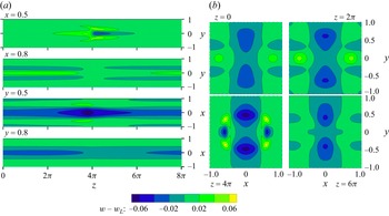


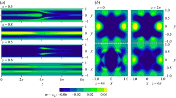


 Open access