


1. Introduction
There is, I think, a widely (though not unanimously) held view among philosophers that Hempel’s (Reference Hempel1945) paradox of the ravens is no more than a historical anecdote because the paradox has already been solved by the Bayesian approach.Footnote 1 We can find this view expressed in some encyclopedic entries on confirmation (Huber Reference Huber2024) and promoted in slides shown to undergraduate students in epistemology or philosophy of science classes. The view that a Bayesian approach can solve the paradox of the ravens, I hope to show, is far from the truth. The Bayesian approaches to the paradox don’t even begin to solve it.
Let’s present the paradox. Take the following seemingly plausible assumptions. First, special cases of a general hypothesis confirm the hypothesis. For example, a black raven is a special case of the hypothesis that all ravens are black, so if we see an object that is a black raven, this fact confirms the hypothesis that all ravens are black. This assumption is referred to as Nicod’s Condition (NC). Second, if evidence E confirms a hypothesis H, and H is logically equivalent to anotherFootnote 2 hypothesis H′, then E confirms H′ too, and to the same degree. This assumption is referred to as the Equivalence Condition (EC). From these seemingly plausible assumptions, we can derive the Paradoxical Conclusion (PC) that the fact we saw, for example, a white shoe confirms the hypothesis that all ravens are black.
The derivation of PC is quite simple. Take the hypothesis H′ stating that all nonblack things are nonravens. A white shoe is a special case of H′, so according to NC, seeing a white shoe confirms H′. But H′ is logically equivalent to H, the hypothesis that all ravens are black. Thus, according to EC, seeing a white shoe also confirms H.
This seems paradoxical because white shoes (and brown tables and green apples) seem completely irrelevant to the color of ravens and learning about the color of shoes doesn’t seem to provide any information about the color of ravens. As Goodman (Reference Goodman1983, 70) quipped, this can seem to give rise to a new field of indoor ornithology. We are left with the dilemma of whether to accept this seemingly paradoxical conclusion or reject one of the premises. If we choose to accept the conclusion, we had better also be able to explain why it seems paradoxical at first sight.
By “the Bayesians,” I shall refer for now to those who choose to accept that both black ravens and nonblack nonravens confirm the hypothesis that all ravens are black, and who therefore accept the seemingly paradoxical conclusion. However, they emphasize that confirmation is a matter of degree, and from the fact that both black ravens and nonblack nonravens confirm the hypothesis that all ravens are black, it doesn’t follow that a nonblack nonraven confirms the hypothesis that all ravens are black to the same degree as a black raven does. In fact, with further assumptions about our prior probabilities of sampling objects from our universe, we can derive the conclusion that the degree of confirmation provided by a nonblack nonraven is negligible compared to the degree of confirmation provided by a black raven. The conclusion seemed paradoxical to us because it did not include further information that the degree of confirmation provided by a nonblack nonraven is negligible. People take nonblack nonravens to be irrelevant to the hypothesis that all ravens are black because they confuse a minute degree of confirmation with zero confirmation. It doesn’t change a great deal in practice.
Thus, in what follows, to qualify as a “Bayesian” solution to the paradox, the two desiderata below need to follow from it:
D 1 : Both sampling a black raven and sampling a nonblack nonraven confirm the hypothesis that all ravens are black.
D 2 : The degree of confirmation provided to the hypothesis that all ravens are black by sampling a nonblack nonraven is negligible compared to the degree of confirmation provided by sampling a black raven.
Some might wonder whether this is too restrictive. It should suffice for a solution to be qualified as “Bayesian” if it uses statistical and probabilistic considerations to solve the paradox, whether they satisfy D 1 and D 2 in the preceding text or not. While indeed the most famous Bayesian solutions satisfy D 1 and D 2 , maybe other solutions that can be qualified as “Bayesian” don’t. I will say something about this issue in the conclusion.
I hope to show that any solution that satisfies D 1 and D 2 suffers from a fatal flaw. The central idea of this article is a rather simple one. A satisfying solution to the Paradox of the Ravens need not only show that the support provided to the hypothesis that all ravens are black by a single nonblack nonraven is negligible compared to the support provided by a single black raven. It also needs to show that the support provided by all the nonblack nonravens we see is negligible compared to the support provided by all the black ravens we see. Otherwise, even if the support provided by a single nonblack nonraven is negligible compared to the support provided by a single black raven, it might be that we see many more nonblack nonravens than black ravens and the cumulative support provided by all the nonblack nonravens we see can be nonnegligible compared to the cumulative support provided by all the black ravens we see. This way, the prospects of indoor ornithology are on the rise, and we are left again in a paradoxical position.
On most Bayesian solutions, what makes it the case that a nonblack nonraven contributes negligibly compared to a black raven is exactly the (obviously true) assumption that it is overwhelmingly more likely when we sample an object at random to sample a nonblack object than to sample a raven. As we shall see in the next section, this assumption implies that it is also overwhelmingly more likely to sample a nonblack nonraven than to sample a black raven. Thus, the attention to the cumulative support provided by all nonblack nonravens we see and all black ravens we see is a natural worry.
If the cumulative support provided by all nonblack nonravens we see is nonnegligible, then the paradox retains its full force. We can still do indoor ornithology and learn about the color of ravens without ever seeing any ravens. To get a feel for the kind of results that will follow, suppose that the cumulative support provided by all the nonblack nonravens I see is equal to the cumulative support provided by all the black ravens I see. Suppose further that my late grandmother, who had similar priors as I have, saw roughly similar things in her life as I did, except that she lived all her life never seeing any raven (or getting any testimony about their color, for that matter). It follows that my grandmother, who was more than twice my age when she passed away, had stronger evidence than I have for the hypothesis that all ravens are black, even though she had never seen any ravens. She probably saw more than double the amount of nonblack nonravens that I saw at the time of her death, and they more than compensate for all the ravens I have seen, and she hadn’t. If the cumulative contribution of all the nonblack nonravens I see is (say) half that of the black ravens, we only need to go back in time to a moment when my grandmother’s age tripled mine (I was old enough to know the color of ravens by then).Footnote 3
Thus, what seems to matter more is not whether a single nonblack nonraven provides a nonnegligible degree of confirmation, but rather whether the cumulative support that all the nonblack nonravens we saw give to the hypothesis that all ravens are black is still negligible compared to the support provided by all the black ravens we saw. The paradox stemmed from the paradoxical flavor of the conclusion that we can learn the color of ravens by looking only at nonblack nonravens. The Bayesians allegedly solved the paradox by showing that under some plausible assumptions, a single nonblack nonraven contributes only negligibly. But it is barely a consolation if, from these very assumptions, it follows that the tons of nonblack nonravens we see will together let us gain substantive confirmation for the claim that ravens are black, without us ever seeing any ravens.
In my view, the need to show that the cumulative support of all the nonblack nonravens is negligible in normal circumstances is part of the difficulty posed by the original paradox, surprisingly unnoticed as it is. Hence the title and my choice of words in the article. Some might contend that this is not part of the original puzzle but rather a separate revenge puzzle. I don’t want to pay too much attention to this matter because nothing crucial hangs on that. It’s open for the readers to defend the Bayesians’ honor and insist that the Bayesians did solve the Paradox of the Ravens, even if I’m right to say that they lack the means to solve an equally disturbing revenge puzzle that stems naturally from the first. The bottom line will remain the same.
To sum up, I take the Paradox of the Ravens to pose another desideratum that must follow from every plausible solution to it:
D 3 : The totality of nonblack nonravens we see contributes negligibly to the confirmation of the hypothesis that all ravens are black compared to the totality of black ravens we see.
To solve the paradox, one needs to derive both D 2 and D 3 from plausible assumptions. The Bayesians want to establish D 1 and D 2 , and they (like everyone else) usually ignore D 3 . I aim to show that, except under some extremely narrow (and usually implausible) assumptions, D 3 is incompatible with D 1 and D 2 . Therefore, to solve the Paradox of the Ravens, that is, to establish D 2 and D 3 , we need to reject D 1 , that is, we need it to be the case that a nonblack nonraven does not positively support the hypothesis that all ravens are black.
Showing that inevitably requires some undergraduate-level calculus. I tried to make it as accessible as possible for readers who are not fluent with these topics, and I have put some of the more technical details in the footnotes and the appendix. In a sense, there is nothing particularly important in the specific mathematical details. The philosophical value of the mathematical details comes from the conclusion they support.
The rest of the article is structured as follows. In the next section, I present the most famous version of a Bayesian solution, sometimes referred to in the literature as the standard, or the canonical, Bayesian solution. This version is adapted from Vranas (Reference Vranas2004) and is the one that, to my impression, is commonly shown to undergraduates in their introductory classes.Footnote 4 In section 3, I show why the assumptions in Vranas’s version imply that (except for extreme conditions) the cumulative contribution of all the nonblack nonravens is not negligible compared to that of the black ravens. In section 4, I explain why that problem is not specific to Vranas’s version. The desiderata D 1 -D 3 can hold together only under implausible conditions. Because the argument for that is more technical, the details are in the appendix. Section 5 is a conclusion.
2. The standard Bayesian solution
The standard Bayesian solution aims to establish D 1 and D 2 from our priors regarding the probabilities of sampling black ravens, nonblack ravens, black nonravens, and nonblack nonravens and from whether and how these probabilities change if the hypothesis that all ravens are black is true. It is common to model the situation as follows: We sample objects from the universe, like drawing balls from an urn. Because we are going to discuss multiple draws in the following text, we will assume we replace the ball we draw back into the urn.Footnote 5 According to the objects we sample (the balls we draw), we try to estimate what the rest of the objects in the universe are (what all the balls in the urn are like). Let’s denote the hypothesis that all ravens are black by H and denote the propositions that the object in question that we have sampled is a black raven, or nonblack raven, or black nonraven, or nonblack nonraven, by br, or nbr, or bnr, or nbnr, accordingly.
We can get all the relevant information regarding the prior probability distribution by specifying the probability of sampling an object from each category conditional on H and conditional on ∼H, and by specifying the prior probability of H. That is, we need to specify the values of all the probabilities in Table 1 and Table 2.
With probability P(H):
Prior probabilities conditional on H
| r | ∼r | |
|---|---|---|
| b | P(br|H) | P(bnr|H) |
| ∼b | P(nbr|H) | P(nbnr|H) |
With probability P(∼H):
Prior probabilities conditional on ∼H
| r | ∼r | |
|---|---|---|
| b | P(br|∼H) | P(bnr|∼H) |
| ∼b | P(bnr|∼H) | P(nbnr|∼H) |
That is, to fully specify our priors, we need the value of the following ten variables: P(br|H), P(nbr|H), P(bnr|H), P(nbnr|H), P(br|∼H), P(nbr|∼H), P(bnr|∼H), P(nbnr|∼H), P(H), and P(∼H).
Not all ten variables are independent. First, of course,
 $P\left( {\sim H} \right) = 1 - P\left( H \right)$
. Moreover,
$P\left( {\sim H} \right) = 1 - P\left( H \right)$
. Moreover,
 $P(br|H) + P(nbr|H) + P(bnr|H) + P(nbnr|H)$
should sum up to one as together the four variables cover the whole universe (conditional on H). Ditto for
$P(br|H) + P(nbr|H) + P(bnr|H) + P(nbnr|H)$
should sum up to one as together the four variables cover the whole universe (conditional on H). Ditto for
 $P(br|{\sim} H) + P(nbr|{\sim} H) + P(bnr|{\sim} H) + P(nbnr|{\sim} H)$
. That is, one in each of these sets of four variables is dependent on the other three. Because P(bnr|H) and P(bnr|∼H) will not play any role in the calculations that follow, we will treat them as the dependent variables. Furthermore, due to the specific meaning of H (i.e., all ravens are black), P(nbr|H) must be zero. Thus, we are left with six independent variables:
$P(br|{\sim} H) + P(nbr|{\sim} H) + P(bnr|{\sim} H) + P(nbnr|{\sim} H)$
. That is, one in each of these sets of four variables is dependent on the other three. Because P(bnr|H) and P(bnr|∼H) will not play any role in the calculations that follow, we will treat them as the dependent variables. Furthermore, due to the specific meaning of H (i.e., all ravens are black), P(nbr|H) must be zero. Thus, we are left with six independent variables:
 $P\left( {br|H} \right),{\rm{ }}P\left( {nbnr|H} \right),{\rm{ }}P\left( {br|{\sim} H} \right),{\rm{ }}P\left( {nbr|{\sim} H} \right),{\rm{ }}P\left( {nbnr|{\sim} H} \right),{\rm{and }}\ P\left( H \right).$
By “independent,” of course, I don’t mean that they can get any value. We are talking about probabilities, so each must range between 0 and 1, and as I said, the probability that an object we sampled is from the whole universe needs to be 1. To avoid triviality and divisions by zero, let’s adopt the common practice and assume that all these six variables are strictly between 0 and 1. The Bayesians aim to solve the paradox for all plausible cases anyway, so surely there is no harm in assuming that.
Note that the probability of sampling a black raven, say, regardless of whether H is true is (according to the law of total probability) simply P(br)=P(H)P(br|H)+P(∼H)P(br|∼H), and ditto for sampling a nonblack raven, black nonraven, or nonblack nonraven. Thus, whenever we see a probability of sampling one of the four categories unconditional on H or ∼H, we can treat it as an abbreviation of an expression that uses only the preceding six variables.
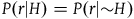
We are now ready to present the standard Bayesian solution. It is common to present it as follows. Our background knowledge, it is claimed, seems to agree with the following three assumptions (nb stands for the proposition that the object in question we have sampled is nonblack, and r stands for it being a raven):Footnote 6
 ${A_1})\;P\left( {nb} \right) \gg P\left( r \right)$
 ${A_2})\;P\left( {r{\rm{|}}H} \right) = P\left( r \right)$
 ${A_3})\;P\left( {nb{\rm{|}}H} \right) = P\left( {nb} \right)$
A
1 states that the probability of sampling a nonblack object at random is overwhelmingly higher than the probability of sampling a raven. A
2
states that the probability of sampling a raven is independent of whether the hypothesis that all ravens are black is true, that is, the probability of sampling a raven conditional on the hypothesis that all ravens are black is simply the probability of sampling a raven in general. A
3
states that the probability of sampling a nonblack object is also independent of the hypothesis that all ravens are black. Note that it’s a direct result of A
2
and A
3
that
 $P\left( {r{\rm{|}}H} \right) = P(r|{\sim} H)$
and
$P\left( {r{\rm{|}}H} \right) = P(r|{\sim} H)$
and
 $P\left( {nb{\rm{|}}H} \right) = P(nb|{\sim} H)$
.Footnote
7
$P\left( {nb{\rm{|}}H} \right) = P(nb|{\sim} H)$
.Footnote
7
These three assumptions suffice to satisfy D
1
and D
2
. There are various ways to show that. It will be useful for what follows to present the case in terms of the preceding six independent variables, so let’s see what each of A
1
-A
3
tells us about them. Let’s denote the ratio
 ${{P\left( {nb} \right)} \over {P\left( r \right)}}$
by m. A
1
tells us that m is a huge number. Note that because both nb and r are probabilistically independent of H (as we learn from A
2
and A
3
), m is independent of whether H is true or not, that is,
${{P\left( {nb} \right)} \over {P\left( r \right)}}$
by m. A
1
tells us that m is a huge number. Note that because both nb and r are probabilistically independent of H (as we learn from A
2
and A
3
), m is independent of whether H is true or not, that is,
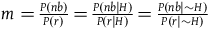 $m = {{P\left( {nb} \right)} \over {P\left( r \right)}} = {{P\left( {nb{\rm{|}}H} \right)} \over {P\left( {r{\rm{|}}H} \right)}} = {{P\left( {nb{\rm{|}}\sim H} \right)} \over {P\left( {r{\rm{|}}\sim H} \right)}}$
. It followsFootnote
8
that:
$m = {{P\left( {nb} \right)} \over {P\left( r \right)}} = {{P\left( {nb{\rm{|}}H} \right)} \over {P\left( {r{\rm{|}}H} \right)}} = {{P\left( {nb{\rm{|}}\sim H} \right)} \over {P\left( {r{\rm{|}}\sim H} \right)}}$
. It followsFootnote
8
that:
 $\;P\left( {nbnr{\rm{|}}H} \right) = mP\left( {br{\rm{|}}H} \right)$
And therefore:
 $\;P(nbnr|H) \gg P(br|H)$
Moreover, it followsFootnote 9 from A 2 and A 3 that:
 $\;P(nbnr|{\sim} H) = mP(br|{\sim} H) + \left( {m - 1} \right)P(nbr|{\sim} H)$
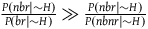
Therefore, P(nbnr|∼H) is at least m times greater than P(br|∼H) and at least (m-1) times greater than P(nbr|∼H). If P(br|∼H) and P(nbr|∼H) are not too small compared to one another, then P(nbnr|∼H) is even more than m times greater than both P(br|∼H) and P(nbr|∼H). That is, we can derive from A 1 both:
 $\;P\left( {nbnr{\rm{|}}{\sim}H} \right) \gg P\left( {br{\rm{|}}{\sim} H} \right)$
 $\;P(nbnr|{\sim} H) \gg P(r|{\sim} H)$
The
 $\gg$
sign is interpreted as at most slightly weaker than the
$\gg$
sign is interpreted as at most slightly weaker than the
 $\gg$
sign in A
1
and in many (perhaps most) cases as even stronger.
$\gg$
sign in A
1
and in many (perhaps most) cases as even stronger.
From A 2 we infer that P(r|H)=P(r|∼H) and therefore we can deriveFootnote 10 that:
 $\;P(br|H) = P(br|{\sim} H) + P(nbr|{\sim} H)$
From A 3 we know that P(nb|H)=P(nb|∼H) and therefore we can similarly deriveFootnote 11 that:
 $\;P(nbnr|H) = P(nbnr|{\sim} H) + P(nbr|{\sim} H)$
Now, there is no single agreed-upon way to measure the degree of confirmation a piece of evidence E confers on a hypothesis H. In the literature (Fitelson and Hawthorne Reference Fitelson, Hawthorne, Eells and James2010a), there are three major relevance measures:
The Difference:
 $\;d\left( {H,E} \right) = P(H|E) - P\left( H \right)$
The Log-Ratio:
 $r\left( {H,E} \right) = \log \left( {{{P\left( {H{\rm{|}}E} \right)} \over {P\left( H \right)}}} \right)$
The Log-Likelihood Ratio:
 $l\left( {H,E} \right) = \log \left( {{{P\left( {E{\rm{|}}H} \right)} \over {P\left( {E{\rm{|}}{\sim} H} \right)}}} \right)$
Among these three, the third one, l, is the most suitable for quantitative comparisons, and there are independent reasons to prefer it (Fitelson Reference Fitelson2001). For this reason, I’ll use this measure in this article.Footnote 12
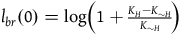
Measured by the log-likelihood ratio, the degrees of confirmation provided to the hypothesis that all ravens are black by a single black raven and by a single nonblack nonraven are:Footnote 13
 $\;{l_{br}} = \log \left( {1 + {{P\left( {nbr{\rm{|}}{\sim} H} \right)} \over {P\left( {br{\rm{|}}{\sim} H} \right)}}} \right)$
 $\;{l_{nbnr}} = \log \left( {1 + {{P\left( {nbr{\rm{|}}{\sim} H} \right)} \over {P\left( {nbnr{\rm{|}}{\sim} H} \right)}}} \right)$
Because all the preceding terms are positive, we see immediately that the confirmation provided by sampling a black raven and by sampling a nonblack nonraven are both positive and therefore both the sampling of a black raven and the sampling of a nonblack nonraven confirm the hypothesis that all ravens are black. Thus, D
1
is satisfied. Furthermore, because
 $P(nbnr|{\sim} H) \gg P(br|{\sim} H)\;$
we get that
$P(nbnr|{\sim} H) \gg P(br|{\sim} H)\;$
we get that
 ${{P\left( {nbr{\rm{|}}{\sim} H} \right)} \over {P\left( {br{\rm{|}}{\sim} H} \right)}} \gg {{P\left( {nbr{\rm{|}}{\sim} H} \right)} \over {P\left( {nbnr{\rm{|}}{\sim} H} \right)}}$
. Therefore, the contribution of a nonblack nonraven is negligible compared to that of a black raven, and D
2
is also satisfied. However, we shall now see that D
3
, in general, cannot be satisfied, except under extreme and implausible assumptions regarding our priors.
${{P\left( {nbr{\rm{|}}{\sim} H} \right)} \over {P\left( {br{\rm{|}}{\sim} H} \right)}} \gg {{P\left( {nbr{\rm{|}}{\sim} H} \right)} \over {P\left( {nbnr{\rm{|}}{\sim} H} \right)}}$
. Therefore, the contribution of a nonblack nonraven is negligible compared to that of a black raven, and D
2
is also satisfied. However, we shall now see that D
3
, in general, cannot be satisfied, except under extreme and implausible assumptions regarding our priors.
3. The nonblack nonravens strike back
To satisfy D 3 , we need to compare the support provided to H by all the black ravens we see and all the nonblack nonravens we see. Because we model each sampling of a black raven or a nonblack nonraven as independent and the log-likelihood ratio is additive, we can compare instead the support H receives from seeing a single black raven, and the support H receives from seeing the number of nonblack nonravens we see per black raven. What is this number?
The expected value of the number of nonblack nonravens we see for each black raven is given by
 ${{P\left( {nbnr} \right)} \over {P\left( {br} \right)}}$
, which under A
1-
A
3
can be rewritten as
${{P\left( {nbnr} \right)} \over {P\left( {br} \right)}}$
, which under A
1-
A
3
can be rewritten as
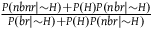 ${{P\left( {nbnr{\rm{|}}{\sim} H} \right) + P\left( H \right)P\left( {nbr{\rm{|}}{\sim} H} \right)} \over {P\left( {br{\rm{|}}{\sim} H} \right) + P\left( H \right)P\left( {nbr{\rm{|}}{\sim} H} \right)}}$
. One can argue that
${{P\left( {nbnr{\rm{|}}{\sim} H} \right) + P\left( H \right)P\left( {nbr{\rm{|}}{\sim} H} \right)} \over {P\left( {br{\rm{|}}{\sim} H} \right) + P\left( H \right)P\left( {nbr{\rm{|}}{\sim} H} \right)}}$
. One can argue that
 ${{P\left( {nbnr} \right)} \over {P\left( {br} \right)}}$
is not the right value to use. We can narrow the discussion to the confirmation provided by all the nonblack nonravens only when it is in fact the case that all ravens are black. In such a scenario, the expected value of the number of nonblack nonravens we see for each black raven is given by
${{P\left( {nbnr} \right)} \over {P\left( {br} \right)}}$
is not the right value to use. We can narrow the discussion to the confirmation provided by all the nonblack nonravens only when it is in fact the case that all ravens are black. In such a scenario, the expected value of the number of nonblack nonravens we see for each black raven is given by
 ${{P\left( {nbnr{\rm{|}}H} \right)} \over {P\left( {br{\rm{|}}H} \right)}}$
that under A
1-
A
3
can be rewritten as
${{P\left( {nbnr{\rm{|}}H} \right)} \over {P\left( {br{\rm{|}}H} \right)}}$
that under A
1-
A
3
can be rewritten as
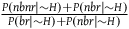 ${{P\left( {nbnr{\rm{|}}{\sim} H} \right) + P\left( {nbr{\rm{|}}{\sim} H} \right)} \over {P\left( {br{\rm{|}}{\sim} H} \right) + P\left( {nbr{\rm{|}}{\sim} H} \right)}}$
, which is smaller than
${{P\left( {nbnr{\rm{|}}{\sim} H} \right) + P\left( {nbr{\rm{|}}{\sim} H} \right)} \over {P\left( {br{\rm{|}}{\sim} H} \right) + P\left( {nbr{\rm{|}}{\sim} H} \right)}}$
, which is smaller than
 ${{P\left( {nbnr} \right)} \over {P\left( {br} \right)}}$
. Taking
${{P\left( {nbnr} \right)} \over {P\left( {br} \right)}}$
. Taking
 ${{P\left( {nbnr{\rm{|}}H} \right)} \over {P\left( {br{\rm{|}}H} \right)}}$
as the expected number simplifies the calculations, and the resulting expected cumulative support of all the nonblack nonravens we see per raven is smaller than if we had taken
${{P\left( {nbnr{\rm{|}}H} \right)} \over {P\left( {br{\rm{|}}H} \right)}}$
as the expected number simplifies the calculations, and the resulting expected cumulative support of all the nonblack nonravens we see per raven is smaller than if we had taken
 ${{P\left( {nbnr} \right)} \over {P\left( {br} \right)}}$
instead as the relevant magnitude. Because I want to be generous toward the Bayesian solution and simplify the calculation, I’ll indeed use
${{P\left( {nbnr} \right)} \over {P\left( {br} \right)}}$
instead as the relevant magnitude. Because I want to be generous toward the Bayesian solution and simplify the calculation, I’ll indeed use
 ${{P\left( {nbnr{\rm{|}}H} \right)} \over {P\left( {br{\rm{|}}H} \right)}}$
as the relevant magnitude (let’s call it choice 1). I’ll sometimes say (in the footnotes, without the full calculation) what is added by taking
${{P\left( {nbnr{\rm{|}}H} \right)} \over {P\left( {br{\rm{|}}H} \right)}}$
as the relevant magnitude (let’s call it choice 1). I’ll sometimes say (in the footnotes, without the full calculation) what is added by taking
 $\;{{P\left( {nbnr} \right)} \over {P\left( {br} \right)}}$
instead (let’s call it choice 2).
$\;{{P\left( {nbnr} \right)} \over {P\left( {br} \right)}}$
instead (let’s call it choice 2).
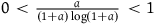
In section (i) of the appendix, I show that under the assumption that each sampling of a nonblack nonraven is independent,Footnote 14 the contribution of this number of nonblack nonravens can be approximated by:Footnote 15
 $\;{l_{nbnr's\;per\;br}} \approx {1 \over {{{P\left( {br{\rm{|}}{\sim} H} \right)} \over {P\left( {nbr{\rm{|}}{\sim} H} \right)}} + 1}}$
The ratio
 ${{P\left( {br{\rm{|}}{\sim} H} \right)} \over {P\left( {nbr{\rm{|}}{\sim} H} \right)}}$
appeared (in its inverse form) in l
br
as well (see 2.8). This ratio tells us what we take in advance the proportion between black ravens and nonblack ravens to be, in case not all ravens are black. For instance, if we think in advance that if not all ravens are black, then half of them are, then the value of this ratio is 1. If we think in advance that if not all ravens are black, then 10 percent of them are, then the value of this ratio is
${{P\left( {br{\rm{|}}{\sim} H} \right)} \over {P\left( {nbr{\rm{|}}{\sim} H} \right)}}$
appeared (in its inverse form) in l
br
as well (see 2.8). This ratio tells us what we take in advance the proportion between black ravens and nonblack ravens to be, in case not all ravens are black. For instance, if we think in advance that if not all ravens are black, then half of them are, then the value of this ratio is 1. If we think in advance that if not all ravens are black, then 10 percent of them are, then the value of this ratio is
 ${1 \over 9}$
. If we think in advance that if not all ravens are black, then either (with a probability of 50 percent) half of them are, or (with a probability of 50 percent) none of them are, then the value of this ratio is
${1 \over 9}$
. If we think in advance that if not all ravens are black, then either (with a probability of 50 percent) half of them are, or (with a probability of 50 percent) none of them are, then the value of this ratio is
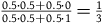 ${{0.5 \cdot 0.5 + 0.5 \cdot 0} \over {0.5 \cdot 0.5 + 0.5 \cdot 1}} = {1 \over 3}$
. In general, I think, we expect this ratio not to be extremely big or extremely small.Footnote
16
At the very least, it seems legitimate to take it in advance to be moderate.
${{0.5 \cdot 0.5 + 0.5 \cdot 0} \over {0.5 \cdot 0.5 + 0.5 \cdot 1}} = {1 \over 3}$
. In general, I think, we expect this ratio not to be extremely big or extremely small.Footnote
16
At the very least, it seems legitimate to take it in advance to be moderate.
For simplicity, let’s denote this ratio by x, that is,
 ${{P\left( {br{\rm{|}}{\sim} H} \right)} \over {P\left( {nbr{\rm{|}}{\sim} H} \right)}} = x$
. We can then rewrite l
br
and l
nbnr’s per br
as
${{P\left( {br{\rm{|}}{\sim} H} \right)} \over {P\left( {nbr{\rm{|}}{\sim} H} \right)}} = x$
. We can then rewrite l
br
and l
nbnr’s per br
as
 ${l_{br}} = \log \left( {1 + {1 \over x}} \right)$
and
${l_{br}} = \log \left( {1 + {1 \over x}} \right)$
and
 ${l_{nbnr's\;per\;br}} = {1 \over {1 + x}}$
.Footnote
17
To satisfy D
3
, we need
${l_{nbnr's\;per\;br}} = {1 \over {1 + x}}$
.Footnote
17
To satisfy D
3
, we need
 ${1 \over {1 + x}}$
to be negligible compared to
${1 \over {1 + x}}$
to be negligible compared to
 $\log \left( {1 + {1 \over x}} \right)$
. One way to formalize this requirement is with the following inequality:
$\log \left( {1 + {1 \over x}} \right)$
. One way to formalize this requirement is with the following inequality:
 $\;{\rm{log}}\left( {1 + {1 \over x}} \right) \gt K\left( {{1 \over {1 + x}}} \right)$
Here
 $K$
is a big negligibility constant. For instance, if to be negligible the value of
$K$
is a big negligibility constant. For instance, if to be negligible the value of
 ${l_{nbnr's\;per\;br}}\;$
needs to be (say) less than 1 percent of the value of
${l_{nbnr's\;per\;br}}\;$
needs to be (say) less than 1 percent of the value of
 ${l_{br}}$
, then
${l_{br}}$
, then
 $K = 99$
. I tend to think that K should be significantly greater than 99, but we don’t need to decide upon it now to proceed. (3.2) is equivalentFootnote
18
to:
$K = 99$
. I tend to think that K should be significantly greater than 99, but we don’t need to decide upon it now to proceed. (3.2) is equivalentFootnote
18
to:
 $\;{\rm{log}}\left( {{{\left( {1 + {1 \over x}} \right)}^{1 + x}}} \right) \gt K$
Exponentiating both sides of the inequality yields:Footnote 19
 $\;{\left( {1 + {1 \over x}} \right)^{1 + x}} \gt {e^K}$
The function
 $f\left( x \right) = {\left( {1 + {1 \over x}} \right)^{1 + x}}$
has been studied in great detail. For our purpose, though, we need only note two things. First, f(x) is descending for every x > 0. Second, (provided that we take K to be greater than 2, say),Footnote
20
the inequality holds for
$f\left( x \right) = {\left( {1 + {1 \over x}} \right)^{1 + x}}$
has been studied in great detail. For our purpose, though, we need only note two things. First, f(x) is descending for every x > 0. Second, (provided that we take K to be greater than 2, say),Footnote
20
the inequality holds for
 $x =1/e^k$
, but fails to hold for
$x =1/e^k$
, but fails to hold for
 $x = 2 /e^k$
. Therefore, for the inequality in (3.4) to hold, x must be smaller than a number that lies somewhere between
$x = 2 /e^k$
. Therefore, for the inequality in (3.4) to hold, x must be smaller than a number that lies somewhere between
 $1/e^k$
and
$1/e^k$
and
 $2/e^k$
. Therefore, to satisfy D
3
, the ratio
$2/e^k$
. Therefore, to satisfy D
3
, the ratio
 ${{P\left( {br{\rm{|}}{\sim} H} \right)}/{P\left( {nbr{\rm{|}}{\sim} H} \right)}}$
must be smaller than
${{P\left( {br{\rm{|}}{\sim} H} \right)}/{P\left( {nbr{\rm{|}}{\sim} H} \right)}}$
must be smaller than
 $2/e^k$
.
$2/e^k$
.
Because K is supposed to be a pretty big number,
 ${e^K}$
should be gigantic.Footnote
21
This means that for the standard Bayesian solution to satisfy D
3
, we must think in advance that if not all ravens are black, and we sample a raven, then the probability that the raven we sample is black should be extremely tiny. To get a feel of how tiny, look at Table 3. The table states how small x should be for some chosen values of K, that is, how likely it is that a given raven we sample is black, conditional on not all ravens being black. To help the reader get a grasp of the magnitudes, in each row, I gave an example of a roughly equiprobable event with which we are more familiar.
${e^K}$
should be gigantic.Footnote
21
This means that for the standard Bayesian solution to satisfy D
3
, we must think in advance that if not all ravens are black, and we sample a raven, then the probability that the raven we sample is black should be extremely tiny. To get a feel of how tiny, look at Table 3. The table states how small x should be for some chosen values of K, that is, how likely it is that a given raven we sample is black, conditional on not all ravens being black. To help the reader get a grasp of the magnitudes, in each row, I gave an example of a roughly equiprobable event with which we are more familiar.
How small x should be for some chosen values of K
| Chosen value of K | The nonblack nonravens contribute at most… | x should be at least smaller than… | Suppose that ∼H and that we have sampled a raven. This raven being black must be less likely than… |
|---|---|---|---|
| 19 | 5% |
 ${2 \over {{e^{19}}}} \approx {10^{ - 8}}$
|
Winning the lotteryFootnote 22 |
| 99 | 1% |
 ${2 \over {{e^{99}}}} \approx {10^{ - 44}}$
|
Winning the lottery six times in a row |
| 999 | 0.1% |
 ${2 \over {{e^{999}}}} \approx {10^{ - 434}}$
|
Randomly sampling the same specific elementary particle from the whole universe five times in a row |
Because ravens are discrete objects and there aren’t that many of them, we get that for the standard Bayesian solution to satisfy D 3 , it must be the case that we think in advance that if not all ravens are black, then it’s overwhelmingly likely that none of them are.Footnote 23 However, there is no reason to think that if not all ravens are black, then none of them are.
Furthermore, remember that the color of ravens is just an example. The paradox seemingly applies to many other properties F and G, and there is even less reason to assume in advance that for all these properties F and G, either all the F’s are G’s or, in probability close to certainty, none or only an unimaginably tiny minority of them are. For example, it seems unreasonable to think we are committed not only to thinking in advance that if not all ravens are black then none of them are but also to thinking in advance that if not all parrots are green then none of them are, if not all chairs have three legs then none of them do, if not all oranges are orange then none of them are, and so forth. I conclude that the standard Bayesian solution cannot plausibly satisfy all three desiderata, and if I’m right in saying that both D 2 and D 3 are crucial to answering the paradox, it follows that the standard Bayesian solution fails to address the paradox of the ravens.Footnote 24
4. The prospects of any alternative Bayesian solution
At this point, the reader might suspect that the challenge I presented applies only to a specific variant of the Bayesian solution, namely, the one presented by Vranas, and while indeed this is probably the most famous version of a Bayesian solution, it needn’t be the only one. What if instead of assumptions A 1 -A 3, we adopt different assumptions? Can’t we then save a Bayesian approach to the paradox of the ravens? My answer is that the prospects for that are not promising, at least when “Bayesian approach” is understood as the strategy of establishing both D 1 and D 2 (i.e., acknowledging that both seeing a black raven and seeing a nonblack nonraven confirm H but a black raven provides stronger support). Making this generalized argument is significantly more complicated than making the preceding argument (though still requires roughly the same level of mathematical proficiency), so I have put the mathematical details in section (iii) of the appendix. Here, I present the general outline of the argument, but I urge the suspicious reader to examine the appendix as well.
The idea of the argument is to examine what follows from adopting the three desiderata D 1 -D 3 , without making any assumptions regarding our background knowledge. That is, recall, we examine what follows from assuming that both seeing a black raven and seeing a nonblack nonraven support the hypothesis that all ravens are black (D 1 ), but the contribution of both a single nonblack nonraven compared to a single black raven (D 2 ), and the aggregate contribution of all the nonblack nonravens we are expected to see compared to the aggregate contribution of all the black ravens we are expected to see (D 3 ) are negligible. We derive that for these three desiderata to hold together, at least one of three conditions must hold, but it is implausible to impose any of these conditions on our priors.
The first condition that allows D
1
-D
3
to hold together states that the ratio
 ${{P\left( {br{\rm{|}}H} \right)} \over {P\left( {br{\rm{|}}{\sim} H} \right)}}$
is extremely big. That is, it is overwhelmingly more likely to sample a black raven if all ravens are black than to sample a black raven if not all of them are, or practically, that if not all ravens are black, then none of them are. Again, there is no reason that our priors regarding ravens must be tuned this way, all the more so our priors regarding any properties F and G for which the paradox applies. Note that this is a generalization of the result we got in the previous section. Earlier, we got from A
1
-A
3
that to satisfy D
1
-D
3
, the ratio
${{P\left( {br{\rm{|}}H} \right)} \over {P\left( {br{\rm{|}}{\sim} H} \right)}}$
is extremely big. That is, it is overwhelmingly more likely to sample a black raven if all ravens are black than to sample a black raven if not all of them are, or practically, that if not all ravens are black, then none of them are. Again, there is no reason that our priors regarding ravens must be tuned this way, all the more so our priors regarding any properties F and G for which the paradox applies. Note that this is a generalization of the result we got in the previous section. Earlier, we got from A
1
-A
3
that to satisfy D
1
-D
3
, the ratio
 ${{P\left( {br{\rm{|}}{\sim} H} \right)} \over {P\left( {nbr{\rm{|}}{\sim} H} \right)}}$
needs to be extremely small, or equivalently, that
${{P\left( {br{\rm{|}}{\sim} H} \right)} \over {P\left( {nbr{\rm{|}}{\sim} H} \right)}}$
needs to be extremely small, or equivalently, that
 ${{P\left( {nbr{\rm{|}}{\sim} H} \right)} \over {P\left( {br{\rm{|}}{\sim} H} \right)}}$
needs to be extremely big. It follows from A
1
-A
3
that
${{P\left( {nbr{\rm{|}}{\sim} H} \right)} \over {P\left( {br{\rm{|}}{\sim} H} \right)}}$
needs to be extremely big. It follows from A
1
-A
3
that
 ${{P\left( {br{\rm{|}}H} \right)} \over {P\left( {br{\rm{|}}{\sim} H} \right)}} \gt {{P\left( {nbr{\rm{|}}{\sim} H} \right)} \over {P\left( {br{\rm{|}}{\sim} H} \right)}}$
so if
${{P\left( {br{\rm{|}}H} \right)} \over {P\left( {br{\rm{|}}{\sim} H} \right)}} \gt {{P\left( {nbr{\rm{|}}{\sim} H} \right)} \over {P\left( {br{\rm{|}}{\sim} H} \right)}}$
so if
 ${{P\left( {nbr{\rm{|}}{\sim} H} \right)} \over {P\left( {br{\rm{|}}{\sim} H} \right)}}$
is extremely big, then so is
${{P\left( {nbr{\rm{|}}{\sim} H} \right)} \over {P\left( {br{\rm{|}}{\sim} H} \right)}}$
is extremely big, then so is
 ${{P\left( {br{\rm{|}}H} \right)} \over {P\left( {br{\rm{|}}{\sim} H} \right)}}$
.
${{P\left( {br{\rm{|}}H} \right)} \over {P\left( {br{\rm{|}}{\sim} H} \right)}}$
.
The second condition that allows D
1
-D
3
to hold together states that
 $P\left( {br{\rm{|}}H} \right) \ge P\left( {nbnr{\rm{|}}H} \right)$
, that is, that if all ravens are black, then sampling a raven is at least as likely as sampling a nonblack object. An implausible condition indeed. This condition comes from the fact that, in the argument presented in the appendix, I assume for convenience that
$P\left( {br{\rm{|}}H} \right) \ge P\left( {nbnr{\rm{|}}H} \right)$
, that is, that if all ravens are black, then sampling a raven is at least as likely as sampling a nonblack object. An implausible condition indeed. This condition comes from the fact that, in the argument presented in the appendix, I assume for convenience that
 ${{P\left( {nbnr{\rm{|}}H} \right)} \over {P\left( {br{\rm{|}}H} \right)}} \gt 1$
, so negating this assumption seemingly lets us evade the conclusion of the argument presented there. In fact, the argument can work with even smaller values than 1,Footnote
25
but it is not crucial. A solution that requires our priors to be such that
${{P\left( {nbnr{\rm{|}}H} \right)} \over {P\left( {br{\rm{|}}H} \right)}} \gt 1$
, so negating this assumption seemingly lets us evade the conclusion of the argument presented there. In fact, the argument can work with even smaller values than 1,Footnote
25
but it is not crucial. A solution that requires our priors to be such that
 $\;P\left( {br{\rm{|}}H} \right) \ge P\left( {nbnr{\rm{|}}H} \right)$
is a nonstarter.
$\;P\left( {br{\rm{|}}H} \right) \ge P\left( {nbnr{\rm{|}}H} \right)$
is a nonstarter.
The third condition that allows D
1
-D
3
to hold is somewhat more complicated, and results from the conclusion of the argument in the appendix (see proposition iii.16). It states, roughly, that for the ratios
 $l = {{P\left( {br{\rm{|}}H} \right)} \over {P\left( {br{\rm{|}}{\sim} H} \right)}},$
 $m = {{P\left( {nbnr{\rm{|}}H} \right)} \over {P\left( {br{\rm{|}}H} \right)}}$
and
$m = {{P\left( {nbnr{\rm{|}}H} \right)} \over {P\left( {br{\rm{|}}H} \right)}}$
and
 $n = {{P\left( {nbnr{\rm{|}}{\sim} H} \right)} \over {P\left( {br{\rm{|}}{\sim} H} \right)}}$
, the following bounds on n must hold:
$n = {{P\left( {nbnr{\rm{|}}{\sim} H} \right)} \over {P\left( {br{\rm{|}}{\sim} H} \right)}}$
, the following bounds on n must hold:
 $\;ml - {l \over K}\log \left( l \right) \lt n \lt ml$
When K is the negligibility constant.
While not easy to see at first glance, this condition is completely implausible. When you look more closely at the inequality in
iii.16, you see that the length of the interval of permissible values for n is dependent only on the values of l and K and independent of the value of m. Suppose, like in the appendix, that (say)
 $l = 10,\;K = 100$
. It follows that the length of the interval of permissible values for n is about 0.23. If
$l = 10,\;K = 100$
. It follows that the length of the interval of permissible values for n is about 0.23. If
 $m = 1000$
, that is, if conditional on all ravens being black, it is 1,000 times more likely to sample a nonblack object than to sample a raven, then n must be in the interval between 10,000 and 10,000 minus 0.23. If
$m = 1000$
, that is, if conditional on all ravens being black, it is 1,000 times more likely to sample a nonblack object than to sample a raven, then n must be in the interval between 10,000 and 10,000 minus 0.23. If
 $m = 1\;billion$
then n must lie in the interval between 10 billion and 10 billion minus 0.23. This is too exact to be taken seriously. The fact that what remains invariant for various values of l, m, and n is the absolute length of the interval rather than its proportional length makes it even more bizarre. D
1
-D
3
severely restrict the set of permissible priors, and in a way that is seemingly hopeless to motivate. At the very least, I can’t see any way to motivate it. Anyone who argues for a solution that maintains D
1
-D
3
needs to provide us with an argument for why our priors must be so fine-tuned.
$m = 1\;billion$
then n must lie in the interval between 10 billion and 10 billion minus 0.23. This is too exact to be taken seriously. The fact that what remains invariant for various values of l, m, and n is the absolute length of the interval rather than its proportional length makes it even more bizarre. D
1
-D
3
severely restrict the set of permissible priors, and in a way that is seemingly hopeless to motivate. At the very least, I can’t see any way to motivate it. Anyone who argues for a solution that maintains D
1
-D
3
needs to provide us with an argument for why our priors must be so fine-tuned.
I conclude that it is not the specific three assumptions A 1 -A 3 of the standard Bayesian solution that get the Bayesians into trouble. It is the very strategy of taking a nonblack nonraven to support the hypothesis that all ravens are black, but only negligibly, that does.
5. Conclusion
The standard Bayesian solution fails because according to it, the aggregate contribution of all the nonblack nonravens we see must be nonnegligible unless we severely and implausibly restrict the set of permissible priors. However, it is not only the standard Bayesian solution that fails. Any solution that wishes to maintain all of the desiderata D 1 -D 3 needs to severely restrict the set of permissible priors in an unmotivated way. Because D 2 -D 3 are desiderata for any solution to the paradox of the ravens, it follows that for a solution to work, D 1 needs to be false. A nonblack nonraven contributes zero or negatively to the confirmation of the hypothesis that all ravens are black. Because there is no reason to think that a nonblack nonraven should disconfirm this hypothesis, the conclusion is that the contribution of a nonblack nonraven to the hypothesis needs to be zero. For some reason, nonblack nonravens (as such) are irrelevant to the confirmation of the hypothesis that all ravens are black.
It is time to discuss the accusation that I have been too restrictive with my use of the term “the Bayesians.” Offering a Bayesian solution to the Paradox of the Ravens, one might protest, does not commit one to adopt D 1 . Rather, it just commits one to solving the paradox using considerations regarding our prior probabilities for sampling black ravens and nonblack nonravens in every scenario.
However, we just saw that any plausible solution to the paradox must take the support provided by a nonblack nonraven to be zero, and only a very specific set of possible prior probability distributions (namely, those in which
 $P\left( {nbnr{\rm{|}}H} \right) = P(nbnr|{\sim} H)$
) give that. There doesn’t seem to be any reason our priors must be like that, a fortiori why they should be like that for every F and G to which the paradox applies. There must be something else in play here beyond our prior statistical beliefs that makes it the case that nonblack nonravens are irrelevant (and that non-F’s non-G’s are irrelevant for F’s and G’s to which the paradox applies). The paradox will not be solved by statistical considerations alone.Footnote
26
If what I said here is correct, the conclusion seems to be that Bayesian considerations alone will not solve the paradox. We need a different strategy.
$P\left( {nbnr{\rm{|}}H} \right) = P(nbnr|{\sim} H)$
) give that. There doesn’t seem to be any reason our priors must be like that, a fortiori why they should be like that for every F and G to which the paradox applies. There must be something else in play here beyond our prior statistical beliefs that makes it the case that nonblack nonravens are irrelevant (and that non-F’s non-G’s are irrelevant for F’s and G’s to which the paradox applies). The paradox will not be solved by statistical considerations alone.Footnote
26
If what I said here is correct, the conclusion seems to be that Bayesian considerations alone will not solve the paradox. We need a different strategy.
Acknowledgments
This article was written under the supervision of Tim Williamson. I thank Tim for his invaluable comments on many versions of the manuscript and for connecting me with Branden Fitelson at a stage when the project was a little more than a vague intuition. I am grateful to Branden for all the effort he put into providing me with very useful background and references, and for his comments on an earlier version. I also thank him for prompting me to generalize the argument I originally had and write section 3 of the appendix. Bernhard Salow became my second supervisor at a later stage of the project, and I thank him for his comments and his help at the revision stage. I thank Ittay Nissan-Rosen for a helpful discussion in the very early stages of the project, and Yotam Dikstein for his endless patience and willingness to help whenever I have a question in mathematics, in this article and in general. I am grateful to Paolo Faglia and Dan Grimmer for their comments on earlier drafts and especially for their meticulous review of the mathematical appendices in search of errors. I thank two anonymous reviewers for this journal for their comments and for verifying the mathematical derivations. Of course, I’m solely responsible for any mathematical error in the text, should there be one. I wish to thank the Reuben Foundation and Reuben College at Oxford for their financial support during the time the article was written. My late grandmother, who features in one of the examples in this article, passed away just days after I wrote down this example. I also wish to use the acknowledgments to commemorate this special woman, who, while focusing on human feelings rather than ornithology, was able to make brilliant inferences from very indirect evidence.
Funding Statement
None to declare.
Declarations
None to declare.
Appendix
-
(i) Calculating the cumulative contribution of many nbnr’s
In this section of the appendix, we calculate the cumulative support of seeing
 ${{P\left( {nbnr{\rm{|}}H} \right)} \over {P\left( {br{\rm{|}}H} \right)}}$
nonblack nonravens.
${{P\left( {nbnr{\rm{|}}H} \right)} \over {P\left( {br{\rm{|}}H} \right)}}$
nonblack nonravens.
 ${{P\left( {nbnr{\rm{|}}H} \right)} \over {P\left( {br{\rm{|}}H} \right)}}$
is not necessarily an integer, but is assumed to be very big, so taking the nearest integer instead should provide practically the same result. We can calculate the degree of confirmation provided by
${{P\left( {nbnr{\rm{|}}H} \right)} \over {P\left( {br{\rm{|}}H} \right)}}$
is not necessarily an integer, but is assumed to be very big, so taking the nearest integer instead should provide practically the same result. We can calculate the degree of confirmation provided by
 ${{P\left( {nbnr{\rm{|}}H} \right)} \over {P\left( {br{\rm{|}}H} \right)}}$
nonblack nonravens as follows (see 2.6 and 2.7):
${{P\left( {nbnr{\rm{|}}H} \right)} \over {P\left( {br{\rm{|}}H} \right)}}$
nonblack nonravens as follows (see 2.6 and 2.7):
 $l{{_{nbnr's\ per\ br}}} = \log \left( \frac{P(nbnr|H)^{{P(nbnr|H)}\over{P(br|H)}}}\over{P(nbnr|\sim H)^{\frac{P(nbnr|H)}\over{P(br|H)}}} \right) = \log \left( \left({P(nbnr|H)}\over{P(nbnr|\sim H)} \right)^{{P(nbnr|H)}\over{P(br|H)}} \right) \\ \,\,\quad\quad\quad\quad= \log \left( \left( 1 + {P(nbr|\sim H)}\over{P(nbnr|\sim H)} \right)^{{P(nbnr|\sim H) + P(nbr|\sim H)}\over{P(br|\sim H) + P(nbr|\sim H)}} \right)$
This expression resembles another, very famous expression. It is well known that
 $\mathop {\lim }\limits_{x \to \infty } {\left( {1 + {1 \over x}} \right)^x} = e$
, and more generally that:
$\mathop {\lim }\limits_{x \to \infty } {\left( {1 + {1 \over x}} \right)^x} = e$
, and more generally that:
 $\;\mathop {\lim }\limits_{x \to \infty } {\left( {1 + a{1 \over x}} \right)^x} = {e^a}$
We know (from 2.3) that
 ${{P\left( {nbnr{\rm{|}}{\sim} H} \right)} \over {P\left( {br{\rm{|}}{\sim} H} \right) + P\left( {nbr{\rm{|}}{\sim} H} \right)}}$
is very large and thus
${{P\left( {nbnr{\rm{|}}{\sim} H} \right)} \over {P\left( {br{\rm{|}}{\sim} H} \right) + P\left( {nbr{\rm{|}}{\sim} H} \right)}}$
is very large and thus
 ${{P\left( {nbr{\rm{|}}{\sim} H} \right)} \over {P\left( {br{\rm{|}}{\sim} H} \right) + P\left( {nbr{\rm{|}}{\sim} H} \right)}}$
only adds a negligible contribution to the term. The expression in (
i.1) can be made very similar to the one in (
i.2) if in the expression
${{P\left( {nbr{\rm{|}}{\sim} H} \right)} \over {P\left( {br{\rm{|}}{\sim} H} \right) + P\left( {nbr{\rm{|}}{\sim} H} \right)}}$
only adds a negligible contribution to the term. The expression in (
i.1) can be made very similar to the one in (
i.2) if in the expression
 ${{P\left( {nbr{\rm{|}}{\sim} H} \right)} \over {P\left( {nbnr{\rm{|}}{\sim} H} \right)}}$
in (
i.1) we multiply both the numerator and the denominator by the factor
${{P\left( {nbr{\rm{|}}{\sim} H} \right)} \over {P\left( {nbnr{\rm{|}}{\sim} H} \right)}}$
in (
i.1) we multiply both the numerator and the denominator by the factor
 $P\left( {br{\rm{|}}{\sim} H} \right) + P\left( {nbr{\rm{|}}{\sim} H} \right)$
:
$P\left( {br{\rm{|}}{\sim} H} \right) + P\left( {nbr{\rm{|}}{\sim} H} \right)$
:
 $\eqalign{& \;\log {\left( {1 + {{P\left( {nbr{\rm{|}}{\sim} H} \right)} \over {P\left( {nbnr{\rm{|}}{\sim} H} \right)}}} \right)^{{{P\left( {nbnr{\rm{|}}{\sim} H} \right) + P\left( {nbr{\rm{|}}{\sim} H} \right)} \over {P\left( {br{\rm{|}}{\sim} H} \right) + P\left( {nbr{\rm{|}}{\sim} H} \right)}}}} \cr & = \log {\left( {1 + {{P\left( {nbr{\rm{|}}{\sim} H} \right)} \over {P\left( {br{\rm{|}}{\sim} H} \right) + P\left( {nbr{\rm{|}}{\sim} H} \right)}}{{P\left( {br{\rm{|}}{\sim} H} \right) + P\left( {nbr{\rm{|}}{\sim} H} \right)} \over {P\left( {nbnr{\rm{|}}{\sim} H} \right)}}} \right)^{{{P\left( {nbnr{\rm{|}}{\sim} H} \right) + P\left( {nbr{\rm{|}}{\sim} H} \right)} \over {P\left( {br{\rm{|}}{\sim} H} \right) + P\left( {nbr{\rm{|}}{\sim} H} \right)}}}} \cr & \approx \log {\left( {1 + {{P\left( {nbr{\rm{|}}{\sim} H} \right)} \over {P\left( {br{\rm{|}}{\sim} H} \right) + P\left( {nbr{\rm{|}}{\sim} H} \right)}}{{P\left( {br{\rm{|}}{\sim} H} \right) + P\left( {nbr{\rm{|}}{\sim} H} \right)} \over {P\left( {nbnr{\rm{|}}{\sim} H} \right)}}} \right)^{{{P\left( {nbnr{\rm{|}}{\sim} H} \right)} \over {P\left( {br{\rm{|}}{\sim} H} \right) + P\left( {nbr{\rm{|}}{\sim} H} \right)}}}} \cr}$
Because
 ${{P\left( {nbr{\rm{|}}{\sim} H} \right)} \over {P\left( {br{\rm{|}}{\sim} H} \right) + P\left( {nbr{\rm{|}}{\sim} H} \right)}}$
is much smaller than
${{P\left( {nbr{\rm{|}}{\sim} H} \right)} \over {P\left( {br{\rm{|}}{\sim} H} \right) + P\left( {nbr{\rm{|}}{\sim} H} \right)}}$
is much smaller than
 ${{P\left( {nbnr{\rm{|}}{\sim} H} \right)} \over {P\left( {br{\rm{|}}{\sim} H} \right) + P\left( {nbr{\rm{|}}{\sim} H} \right)}}$
, we can now use (
i.2) to approximate the last expression in (
i.3) as:
${{P\left( {nbnr{\rm{|}}{\sim} H} \right)} \over {P\left( {br{\rm{|}}{\sim} H} \right) + P\left( {nbr{\rm{|}}{\sim} H} \right)}}$
, we can now use (
i.2) to approximate the last expression in (
i.3) as:
 $\log \left( {{e^{{{P\left( {nbr{\rm{|}}{\sim} H} \right)} \over {P\left( {br{\rm{|}}{\sim} H} \right) + P\left( {nbr{\rm{|}}{\sim} H} \right)}}}}} \right)$
And this last term in ( i.4) is equal to:
 $\;\log \left( {{e^{{{P\left( {nbr{\rm{|}}{\sim} H} \right)} \over {P\left( {br{\rm{|}}{\sim} H} \right) + P\left( {nbr{\rm{|}}{\sim} H} \right)}}}}} \right) = {{P\left( {nbr{\rm{|}}{\sim} H} \right)} \over {P\left( {br{\rm{|}}{\sim} H} \right) + P\left( {nbr{\rm{|}}{\sim} H} \right)}} = {1 \over {{{P\left( {br{\rm{|}}{\sim} H} \right)} \over {P\left( {nbr{\rm{|}}{\sim} H} \right)}} + 1}}$
In the end, we get that:
 $\;{l_{nbnr's\;per\;br}} \approx {1 \over {{{P\left( {br{\rm{|}}{\sim} H} \right)} \over {P\left( {nbr{\rm{|}}{\sim} H} \right)}} + 1}}$
Which is what we wanted to demonstrate.
-
(ii) Sampling without replacement
In this section of the appendix, I show that given two reasonable assumptions, modeling the situation as sampling without replacement does not cause significant divergence from modeling the situation as sampling with replacement. I present only the case for the cumulative contribution of all black ravens the subject sees. The case for the cumulative contribution of all nonblack nonravens the subject sees is analogous.
The first assumption is that the subject believes that the number of objects in the universe depends only negligibly on whether all ravens are black or not. That is, if N
H
stands for the believed number of objects in the universe conditional on H, and N
∼H
is the believed number of objects in the universe conditional on ∼H, then for all practical purposes, we can assume that
 ${N_H} = {N_{{\sim} H}} = N$
.Footnote
27
Of course, the subject might assign prior probabilities to various values of N, but we assume that for each specific value of N, the probability for this value of N is, for all practical purposes, independent of H. Thus, we can treat N as a specific number, and the argument generalizes for a probability distribution for values of N.
${N_H} = {N_{{\sim} H}} = N$
.Footnote
27
Of course, the subject might assign prior probabilities to various values of N, but we assume that for each specific value of N, the probability for this value of N is, for all practical purposes, independent of H. Thus, we can treat N as a specific number, and the argument generalizes for a probability distribution for values of N.
Suppose then that the subject’s prior belief is that there are N objects in the universe. Let
 ${K_H}$
stand for the number of black ravens the subject believes there are in the universe in case H is true, and let
${K_H}$
stand for the number of black ravens the subject believes there are in the universe in case H is true, and let
 ${K_{{\sim} H}}$
stand for the number of black ravens the subject believes there are in the universe in case H is false (note,
${K_{{\sim} H}}$
stand for the number of black ravens the subject believes there are in the universe in case H is false (note,
 ${K_H}$
and
${K_H}$
and
 ${K_{{\sim} H}}\;$
have nothing to do with the negligibility constant K introduced previously). We can express the subject prior conditional probability for sampling a black raven on the first draw as
${K_{{\sim} H}}\;$
have nothing to do with the negligibility constant K introduced previously). We can express the subject prior conditional probability for sampling a black raven on the first draw as
 $P\left( {br{\rm{|}}H} \right) = {{{K_H}} \over N},\;P\left( {br{\rm{|}}{\sim} H} \right) = {{{K_{{\sim} H}}} \over N}$
. The log-likelihood ratio before the first draw (i.e., after 0 draws) is:
$P\left( {br{\rm{|}}H} \right) = {{{K_H}} \over N},\;P\left( {br{\rm{|}}{\sim} H} \right) = {{{K_{{\sim} H}}} \over N}$
. The log-likelihood ratio before the first draw (i.e., after 0 draws) is:
 $l_{br}(0)=\log\left({K_H/N}\over{K_{\sim H}/N}\right)=\log\left({K_H}\over{K_{\sim H}}\right)$
Note that according to D
1,
the contribution of seeing a black raven should be positive, so
 ${K_H}$
should be greater than
${K_H}$
should be greater than
 ${K_{{\sim} H}}$
.Footnote
28
Let n stand for the number of objects sampled so far, and k stand for the number of black ravens sampled so far. In general, the log likelihood ratio of seeing one black raven after seeing n objects and k black ravens without replacement is
${K_{{\sim} H}}$
.Footnote
28
Let n stand for the number of objects sampled so far, and k stand for the number of black ravens sampled so far. In general, the log likelihood ratio of seeing one black raven after seeing n objects and k black ravens without replacement is
 $\log {{(K_H - k) / (N - n)}\over{(K_{\sim H} - k) / (N - n)}}$
. The N-n cancels out, so the contribution of seeing each new black raven is a function of k alone. That is, the contribution of seeing a black raven after sampling k black ravens (i.e., the contribution of the (k+1)th black raven) is:
$\log {{(K_H - k) / (N - n)}\over{(K_{\sim H} - k) / (N - n)}}$
. The N-n cancels out, so the contribution of seeing each new black raven is a function of k alone. That is, the contribution of seeing a black raven after sampling k black ravens (i.e., the contribution of the (k+1)th black raven) is:
 $\;{l_{br}}\left( k \right) = \log {{{K_H} - k} \over {{K_{{\sim} H}} - k}}$
Note that for each k,
 ${l_{br}}\left( k \right)$
can be decomposed to:Footnote
29
${l_{br}}\left( k \right)$
can be decomposed to:Footnote
29
 $\;{l_{br}}\left( k \right) = \log {{{K_H}} \over {{K_{{\sim} H}}}} + \log {{\left( {1 - {k \over {{K_{}}}}} \right)} \over {\left( {1 - {k \over {{K_{{\sim} H}}}}} \right)}}$
The left-hand side is just
 ${l_{br}}\left( 0 \right)$
and the right-hand side is a correction term that is a function of k. Let’s call it Corr(k).
${l_{br}}\left( 0 \right)$
and the right-hand side is a correction term that is a function of k. Let’s call it Corr(k).
 $\;Corr\left( k \right) = \log {{\left( {1 - {k \over {{K_H}}}} \right)} \over {\left( {1 - {k \over {{K_{{\sim} H}}}}} \right)}}$
That is,
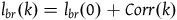 ${l_{br}}\left( k \right) = {l_{br}}\left( 0 \right) + Corr\left( k \right)$
. The cumulative contribution of seeing k black ravens with replacement is just
${l_{br}}\left( k \right) = {l_{br}}\left( 0 \right) + Corr\left( k \right)$
. The cumulative contribution of seeing k black ravens with replacement is just
 $k{l_{br}}\left( 0 \right)$
. Without replacement, the cumulative contribution of seeing k black ravens is:Footnote
30
$k{l_{br}}\left( 0 \right)$
. Without replacement, the cumulative contribution of seeing k black ravens is:Footnote
30
 $\;\mathop \sum \limits_0^{k - 1} {l_{br}}\left( 0 \right) + Corr\left( k \right) = k{l_{br}}\left( 0 \right) + \mathop \sum \limits_0^{k - 1} Corr\left( k \right)$
The second assumption I’m making is that the total number of black ravens the subject sees, call it
 ${k_0}$
, is small compared to the total number of black ravens, whether all ravens are black or not. That is,
${k_0}$
, is small compared to the total number of black ravens, whether all ravens are black or not. That is,
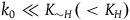 ${k_0} \ll {K_{{\sim} H}}( \lt {K_H})$
. If the subject sees
${k_0} \ll {K_{{\sim} H}}( \lt {K_H})$
. If the subject sees
 ${k_0}$
black ravens, the divergence between their cumulative contribution with and without replacement is
${k_0}$
black ravens, the divergence between their cumulative contribution with and without replacement is
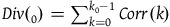 $Div\left( {_0} \right) = \mathop \sum \nolimits_{k = 0}^{{k_0} - 1} Corr\left( k \right)$
. If
$Div\left( {_0} \right) = \mathop \sum \nolimits_{k = 0}^{{k_0} - 1} Corr\left( k \right)$
. If
 ${k_0}$
is small compared to
${k_0}$
is small compared to
 ${K_{{\sim} H}}$
, then for every
${K_{{\sim} H}}$
, then for every
 $k \lt {k_0}$
,
$k \lt {k_0}$
,
 $Corr\left( k \right)$
can be approximated by:Footnote
31
$Corr\left( k \right)$
can be approximated by:Footnote
31
 $\;Corr\left( k \right) \approx \;{k \over {{K_{{\sim} H}}}} - {k \over {{K_H}}}$
Therefore, the total divergence after seeing
 ${k_0}$
black ravens is:Footnote
32
${k_0}$
black ravens is:Footnote
32
 $\;Div\left( {{k_0}} \right) \approx \left( {{{\;{k_0}\left( {{k_0} - 1} \right)} \over 2}} \right)\left( {{1 \over {{K_{{\sim} H}}}} - {1 \over {{K_H}}}} \right)$
To understand how big the divergence is, we need to compare
 $Div\left( {{k_0}} \right)$
with the cumulative contribution with replacement,
$Div\left( {{k_0}} \right)$
with the cumulative contribution with replacement,
 ${k_0}{l_{br}}\left( 0 \right)$
. To do that, note that
${k_0}{l_{br}}\left( 0 \right)$
. To do that, note that
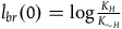 ${l_{br}}\left( 0 \right) = \log {{{K_H}} \over {{K_{{\sim} H}}}}$
can be rewritten as
${l_{br}}\left( 0 \right) = \log {{{K_H}} \over {{K_{{\sim} H}}}}$
can be rewritten as
 ${l_{br}}\left( 0 \right) = \log \left( {1 + {{{K_H} - {K_{{\sim} H}}} \over {{K_{{\sim} H}}}}} \right)$
. Define:
${l_{br}}\left( 0 \right) = \log \left( {1 + {{{K_H} - {K_{{\sim} H}}} \over {{K_{{\sim} H}}}}} \right)$
. Define:
 ${{{K_H} - {K_{{\sim} H}}} \over {{K_{{\sim} H}}}} = a$
. Note that
${{{K_H} - {K_{{\sim} H}}} \over {{K_{{\sim} H}}}} = a$
. Note that
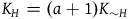 ${K_H} = \left( {a + 1} \right){K_{{\sim} H}}$
. We can then rewrite
${K_H} = \left( {a + 1} \right){K_{{\sim} H}}$
. We can then rewrite
 ${k_0}{l_{br}}\left( 0 \right)$
as
${k_0}{l_{br}}\left( 0 \right)$
as
 ${k_0}\log \left( {1 + a} \right)$
and rewrite
${k_0}\log \left( {1 + a} \right)$
and rewrite
 $Div\left( {{k_0}} \right)$
as
$Div\left( {{k_0}} \right)$
as
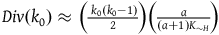 $Div\left( {{k_0}} \right) \approx \left( {{{\;{k_0}\left( {{k_0} - 1} \right)} \over 2}} \right)\left( {{a \over {\left( {a + 1} \right){K_{{\sim} H}}}}} \right)$
. We can then express the ratio between
$Div\left( {{k_0}} \right) \approx \left( {{{\;{k_0}\left( {{k_0} - 1} \right)} \over 2}} \right)\left( {{a \over {\left( {a + 1} \right){K_{{\sim} H}}}}} \right)$
. We can then express the ratio between
 $Div\left( {{k_0}} \right)$
and
$Div\left( {{k_0}} \right)$
and
 ${k_0}{l_{br}}\left( 0 \right)$
as:
${k_0}{l_{br}}\left( 0 \right)$
as:
 $\;{{Div\left( {{k_0}} \right)} \over {{k_0}{l_{br}}\left( 0 \right)}} \approx {a \over {\left( {1 + a} \right)\log \left( {1 + a} \right)}}{{{k_0} - 1} \over {2{K_{{\sim} H}}}}$
Because
 $0 \lt {a \over {\left( {1 + a} \right)\log \left( {1 + a} \right)}} \lt 1$
for every
$0 \lt {a \over {\left( {1 + a} \right)\log \left( {1 + a} \right)}} \lt 1$
for every
 $a \gt 0$
and
$a \gt 0$
and
 ${k_0} \ll {K_{{\sim} H}}$
, we get that
${k_0} \ll {K_{{\sim} H}}$
, we get that
 $Div\left( {{k_0}} \right)$
is small compared to
$Div\left( {{k_0}} \right)$
is small compared to
 ${k_0}{l_{br}}\left( 0 \right).$
That is, given the assumptions that the subject takes the total number of objects in the universe to be independent from the hypothesis that all ravens are black and that the subject only sees a small subset of all black ravens, the divergence between modeling the situation as sampling with replacement and sampling without replacement is small. Therefore, modeling the situation as sampling without replacement is unlikely to change the overall verdict.
${k_0}{l_{br}}\left( 0 \right).$
That is, given the assumptions that the subject takes the total number of objects in the universe to be independent from the hypothesis that all ravens are black and that the subject only sees a small subset of all black ravens, the divergence between modeling the situation as sampling with replacement and sampling without replacement is small. Therefore, modeling the situation as sampling without replacement is unlikely to change the overall verdict.
-
(iii) D 1 - D 3 without A 1 -A 3
Suppose we don’t adopt any assumptions about our background knowledge, but we want all the desiderata D 1 -D 3 to hold. These three desiderata, it turns out, are only consistent with a narrow set of possible priors, and I don’t think there is any independent argument for why we need to have these specific priors. Let’s see why.
As we saw previously, the degree of confirmation provided by a single black raven is
 $\log \left( {{{P\left( {br{\rm{|}}H} \right)} \over {P\left( {br{\rm{|}}{\sim} H} \right)}}} \right)$
and the degree of confirmation provided by a single nonblack nonraven is
$\log \left( {{{P\left( {br{\rm{|}}H} \right)} \over {P\left( {br{\rm{|}}{\sim} H} \right)}}} \right)$
and the degree of confirmation provided by a single nonblack nonraven is
 $\log \left( {{{P\left( {nbnr{\rm{|}}H} \right)} \over {P\left( {nbnr{\rm{|}}{\sim} H} \right)}}} \right)$
. The first and the second desiderata imply together that:Footnote
33
$\log \left( {{{P\left( {nbnr{\rm{|}}H} \right)} \over {P\left( {nbnr{\rm{|}}{\sim} H} \right)}}} \right)$
. The first and the second desiderata imply together that:Footnote
33
 $\;{\rm{log}}\left( {{{P\left( {br{\rm{|}}H} \right)} \over {P\left( {br{\rm{|}}{\sim} H} \right)}}} \right) \gt \log \left( {{{P\left( {nbnr{\rm{|}}H} \right)} \over {P\left( {nbnr{\rm{|}}{\sim} H} \right)}}} \right) \gt 0$
Or, equivalently, that:
 $\;{{P\left( {br{\rm{|}}H} \right)} \over {P\left( {br{\rm{|}}{\sim} H} \right)}} \gt {{P\left( {nbnr{\rm{|}}H} \right)} \over {P\left( {nbnr{\rm{|}}{\sim} H} \right)}} \gt 1$
To simplify, let’s say (as in section 4) that
 ${{P\left( {nbnr{\rm{|}}H} \right)} \over {P\left( {br{\rm{|}}H} \right)}} = m$
and that
${{P\left( {nbnr{\rm{|}}H} \right)} \over {P\left( {br{\rm{|}}H} \right)}} = m$
and that
 ${{P\left( {nbnr{\rm{|}}{\sim} H} \right)} \over {P\left( {br{\rm{|}}{\sim} H} \right)}} = n\;$
. We can then infer from (
iii.2) that:
${{P\left( {nbnr{\rm{|}}{\sim} H} \right)} \over {P\left( {br{\rm{|}}{\sim} H} \right)}} = n\;$
. We can then infer from (
iii.2) that:
 $\;n = {{P\left( {nbnr{\rm{|}}{\sim} H} \right)} \over {P\left( {br{\rm{|}}{\sim} H} \right)}} \gt {{P\left( {nbnr{\rm{|}}H} \right)} \over {P\left( {br{\rm{|}}H} \right)}} = m$
And that:
 $\;{{P\left( {br{\rm{|}}H} \right)} \over {P\left( {br{\rm{|}}{\sim} H} \right)}} \gt {{mP\left( {br{\rm{|}}H} \right)} \over {nP\left( {br{\rm{|}}{\sim} H} \right)}} \gt 1$
We tend to think that both m and n need to be very big, but we won’t need this assumption for what follows. All we will need is that m won’t be very small. It is useful though to think of m as at least greater than 1, that is, that according to our priors, given that all ravens are black, it is at least as likely to sample a nonblack nonraven as it is to sample a black raven (which, conditional on all ravens being black, is equivalent to the claim that it is at least as likely to sample a nonblack object as it is to sample a raven). What I say in the text that follows can work with values of m that are even smaller than 1, but in any case, any solution to the paradox of the ravens should be compatible with m being more than 1. The ratio
 ${{P\left( {br{\rm{|}}H} \right)} \over {P\left( {br{\rm{|}}{\sim} H} \right)}}$
will be used many times in what follows. For convenience, let’s substitute it with the single letter l (for “likelihood”), that is,
${{P\left( {br{\rm{|}}H} \right)} \over {P\left( {br{\rm{|}}{\sim} H} \right)}}$
will be used many times in what follows. For convenience, let’s substitute it with the single letter l (for “likelihood”), that is,
 ${{P\left( {br{\rm{|}}H} \right)} \over {P\left( {br{\rm{|}}{\sim} H} \right)}} = l$
.Footnote
34
Note that it follows from (4) that
${{P\left( {br{\rm{|}}H} \right)} \over {P\left( {br{\rm{|}}{\sim} H} \right)}} = l$
.Footnote
34
Note that it follows from (4) that
 ${m \over n}l \gt 1$
, or, equivalently, that
${m \over n}l \gt 1$
, or, equivalently, that
 ${n \over m} \lt l$
Note that (
iii.5) is in effect just another way to say that
 $P\left( {nbnr{\rm{|}}{\sim} H} \right) \lt P(nbnr|H)$
, or that
$P\left( {nbnr{\rm{|}}{\sim} H} \right) \lt P(nbnr|H)$
, or that
 ${{P\left( {nbnr{\rm{|}}H} \right)} \over {P\left( {nbnr{\rm{|}}{\sim} H} \right)}} \gt 1$
, as we already know from (
iii.2).
${{P\left( {nbnr{\rm{|}}H} \right)} \over {P\left( {nbnr{\rm{|}}{\sim} H} \right)}} \gt 1$
, as we already know from (
iii.2).
Let’s turn now to D
3
. If H is true, we expect to see m nonblack nonravens for each black raven. If H is false, we expect to see n nonblack nonravens for each black raven. The expected value for the number of nonblack nonravens we see per each black raven is
 $mP\left( H \right) + nP\left( {{\sim} H} \right)$
, which is greater than m, because n > m. Therefore, taking m as the expected value of the number of nonblack nonravens we see per each black raven is again generous toward the Bayesians. To satisfy D
3
, we need that:
$mP\left( H \right) + nP\left( {{\sim} H} \right)$
, which is greater than m, because n > m. Therefore, taking m as the expected value of the number of nonblack nonravens we see per each black raven is again generous toward the Bayesians. To satisfy D
3
, we need that:
 ${\rm{log}}\left( {{{P\left( {br{\rm{|}}H} \right)} \over {P\left( {br{\rm{|}}{\sim} H} \right)}}} \right) \gt K\log {\left( {{{P\left( {nbnr{\rm{|}}H} \right)} \over {P\left( {nbnr{\rm{|}}{\sim} H} \right)}}} \right)^m}$
Or, equivalently:
 $\;\log \left( l \right){\rm{ \gt Klog}}{\left( {{m \over n}l} \right)^m} = mK\log \left( {{m \over n}l} \right) = mK\left( {\log \left( {{m \over n}} \right) + \log \left( l \right)} \right)$
Where K is again a negligibility constant that is supposed to be pretty big. Rearranging ( iii.7) gives us:
 $\;\left( {mK - 1} \right)\log \left( l \right) \lt - mK\log \left( {{m \over n}} \right) = mK\log \left( {{n \over m}} \right)$
Which in turn gives:
 $\;{{mK - 1} \over {mK}}\log \left( l \right) = \left( {1 - {1 \over {mK}}} \right)\log \left( l \right) = \log ({l^{1 - {1 \over {mK}}}}){\rm{ \lt }}\log \left( {{n \over m}} \right)$
Exponentiating ( iii.9) gives:
 $\;{n \over m} \gt {\left( l \right)^{1 - {1 \over {mK}}}}$
( iii.5) and ( iii.10) together yield:
 $\;{l^{1 - {1 \over {mK}}}} \lt {n \over m} \lt l$
To be more systematic, we can separate n and rewrite ( iii.11) as:
 $\;m{l^{1 - {1 \over {mK}}}} \lt n \lt ml$
That is, to answer desiderata D
1
-D
3
, our prior value for
 $n$
(i.e., recall, our prior value for the ratio
$n$
(i.e., recall, our prior value for the ratio
 ${{P\left( {nbnr{\rm{|}}{\sim} H} \right)} \over {P\left( {br{\rm{|}}{\sim} H} \right)}}$
) needs to be bounded within an interval, which in cases in which K is big, and m is big compared to
${{P\left( {nbnr{\rm{|}}{\sim} H} \right)} \over {P\left( {br{\rm{|}}{\sim} H} \right)}}$
) needs to be bounded within an interval, which in cases in which K is big, and m is big compared to
 ${1 \over K}$
, is a very narrow one. If m is significantly bigger than
${1 \over K}$
, is a very narrow one. If m is significantly bigger than
 ${1 \over K}$
then the difference between
${1 \over K}$
then the difference between
 $l$
and
$l$
and
 ${l^{1 - {1 \over {mK}}}}$
is tiny. To get a feel of how narrow the interval between them should be, suppose (say) that
${l^{1 - {1 \over {mK}}}}$
is tiny. To get a feel of how narrow the interval between them should be, suppose (say) that
 $l = 10,\;K = 100,\;and\;m = 1000$
. In such a case, we get that
$l = 10,\;K = 100,\;and\;m = 1000$
. In such a case, we get that
 $9,999.77 \approx 1000 \cdot {10^{{{99,999} \over {100,000}}}} \lt n \lt 1000 \cdot 10 = 10,000$
.
$9,999.77 \approx 1000 \cdot {10^{{{99,999} \over {100,000}}}} \lt n \lt 1000 \cdot 10 = 10,000$
.
The difference between the expression on the right-hand side of (
iii.12) and the expression on the left-hand side of (
iii.12) is
 $ml - m{l^{1 - {1 \over {mK}}}} = m\left( {l - {l^{1 - {1 \over {mK}}}}} \right)$
. If m is significantly bigger than
$ml - m{l^{1 - {1 \over {mK}}}} = m\left( {l - {l^{1 - {1 \over {mK}}}}} \right)$
. If m is significantly bigger than
 ${1 \over K}$
, then
${1 \over K}$
, then
 ${1 \over {mK}}$
is a pretty small number. Therefore,
${1 \over {mK}}$
is a pretty small number. Therefore,
 $l - {l^{1 - {1 \over {mK}}}}$
can be approximated using the Taylor expansion near zero of
$l - {l^{1 - {1 \over {mK}}}}$
can be approximated using the Taylor expansion near zero of
 ${l^{1 - x}}$
where we take
${l^{1 - x}}$
where we take
 $x = {1 \over {mK}}$
as our variable. (
iii.12) presents the Taylor expansion of
$x = {1 \over {mK}}$
as our variable. (
iii.12) presents the Taylor expansion of
 ${l^{1 - x}}$
near
${l^{1 - x}}$
near
 $x = 0$
:
$x = 0$
:
 $\eqalign{ & {l^{1 - x}} = {e^{\log \left( l \right)\left( {1 - x} \right)}} \cr & \,\,\,\quad\;\, = {e^{\log \left( l \right)\left( {1 - 0} \right)}} - \log \left( l \right){e^{\log \left( l \right)\left( {1 - 0} \right)}}x + {1 \over 2}{\log ^2}\left( l \right){e^{\log \left( l \right)\left( {1 - 0} \right)}}{x^2} + \ldots \cr & \,\,\,\quad\;\, = l - \log \left( l \right) \cdot lx + {1 \over 2}{\log ^2}\left( l \right) \cdot l{x^2} + \ldots \approx l - \log \left( l \right) \cdot l \cdot {1 \over {mK}}}$
The approximation at the end of (
iii.13) is derived from the fact that because
 $x = {1 \over {mK}}$
is close to zero, the higher powers of x are very small compared to x (and we assume that l is not gigantic enough for the coefficients to compensate). It follows from the approximation in (
iii.12) that:
$x = {1 \over {mK}}$
is close to zero, the higher powers of x are very small compared to x (and we assume that l is not gigantic enough for the coefficients to compensate). It follows from the approximation in (
iii.12) that:
 $\;l - {l^{1 - {1 \over {mK}}}} \approx \log \left( l \right) \cdot l \cdot {1 \over {mK}}$
Therefore,
 $\;m\left( {l - {l^{1 - {1 \over {mK}}}}} \right) \approx {\rm{mlog}}\left( l \right) \cdot l \cdot {1 \over {mK}} = {l \over K}\log \left( l \right)$
That is, ( iii.12) can be rewritten approximately as:
 $\;ml - {l \over K}\log \left( l \right) \lt n \lt ml$
What can be learned from this? First, we see that the length of the interval of permissible values for n is approximately independent of m. In the preceding case, where
 $l = 10,\;K = 100,$
it always has a length of about 0.23. That is, if (say)
$l = 10,\;K = 100,$
it always has a length of about 0.23. That is, if (say)
 $m = 2$
, then n must lie in the interval between 20 (i.e., ml) and 20 minus 0.23. If
$m = 2$
, then n must lie in the interval between 20 (i.e., ml) and 20 minus 0.23. If
 $m = 1000$
(as we saw in the preceding text), n must lie in the interval between 10,000 and 10,000 minus 0.23. If
$m = 1000$
(as we saw in the preceding text), n must lie in the interval between 10,000 and 10,000 minus 0.23. If
 $m = 1\;billion$
then n must lie in the interval between 10 billion and 10 billion minus 0.23.
$m = 1\;billion$
then n must lie in the interval between 10 billion and 10 billion minus 0.23.
Second, it’s reasonable to assume that K is determined independently of the specifics of the setting of the paradox. K, after all, is a negligibility constant, that is, it should determine only when the contribution of a piece of evidence e is negligible. It should have nothing to do specifically with our priors regarding ravens. Therefore, it seems that l is the only flexible value in
 ${l \over k}\log \left( l \right)$
, and we can see that
${l \over k}\log \left( l \right)$
, and we can see that
 ${l \over k}\log \left( l \right)$
becomes bigger the bigger l is. This is in accord with what we have found about the canonical Bayesian solution. l, recall, is the ratio
${l \over k}\log \left( l \right)$
becomes bigger the bigger l is. This is in accord with what we have found about the canonical Bayesian solution. l, recall, is the ratio
 ${{P\left( {br{\rm{|}}H} \right)} \over {P\left( {br{\rm{|}}{\sim} H} \right)}}$
, and if l is very big, it implies that the probability of sampling a black raven in case H is false is tiny compared to the probability of sampling a black raven in case H is true. However, for reasonable values of l, we get that the interval of possible values for n is very narrow and independent of the probabilities of sampling a nonblack nonraven or a black raven.
${{P\left( {br{\rm{|}}H} \right)} \over {P\left( {br{\rm{|}}{\sim} H} \right)}}$
, and if l is very big, it implies that the probability of sampling a black raven in case H is false is tiny compared to the probability of sampling a black raven in case H is true. However, for reasonable values of l, we get that the interval of possible values for n is very narrow and independent of the probabilities of sampling a nonblack nonraven or a black raven.
Another point to note is that when we unpack the notation in the inequality ( iii.16) back to our original variables, we see that it can be rewritten as:
 $\;P\left( {nbnr{\rm{|}}H} \right) - {{P\left( {br{\rm{|}}H} \right)} \over K}\log \left( {{{P\left( {br{\rm{|}}H} \right)} \over {P\left( {br{\rm{|}}{\sim} H} \right)}}} \right) \lt P\left( {nbnr{\rm{|}}{\sim} H} \right) \lt P\left( {nbnr{\rm{|}}H} \right)$
That is, while greater l indeed implies a greater length of the interval of possible values for
 $\left( {nbnr{\rm{|}}{\sim} H} \right)$
, because in any case
$\left( {nbnr{\rm{|}}{\sim} H} \right)$
, because in any case
 $P\left( {br{\rm{|}}H} \right) \lt 1$
, and therefore in any case
$P\left( {br{\rm{|}}H} \right) \lt 1$
, and therefore in any case
 ${{P\left( {br{\rm{|}}H} \right)} \over K} \lt {1 \over k},\;$
the growth in l contributes almost entirely logarithmically to the growth of the interval of possible values for
${{P\left( {br{\rm{|}}H} \right)} \over K} \lt {1 \over k},\;$
the growth in l contributes almost entirely logarithmically to the growth of the interval of possible values for
 $P\left( {nbnr{\rm{|}}{\sim} H} \right)$
. That is, to widen the interval of possible values for
$P\left( {nbnr{\rm{|}}{\sim} H} \right)$
. That is, to widen the interval of possible values for
 $P\left( {nbnr{\rm{|}}{\sim} H} \right)$
just by a tiny bit, l will need to grow by a great deal. If l is not too big, then as I explain in section 4, this result poses an implausible and somewhat bizarre restriction on the set of permissible priors.
$P\left( {nbnr{\rm{|}}{\sim} H} \right)$
just by a tiny bit, l will need to grow by a great deal. If l is not too big, then as I explain in section 4, this result poses an implausible and somewhat bizarre restriction on the set of permissible priors.


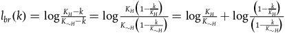


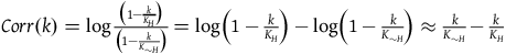
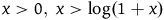


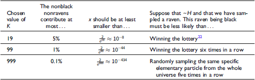

 Open access