


1 Introduction
While stellarators offer the possibility of stable, steady-state fusion power with minimal recirculating power and immunity from disruptions, particle confinement in stellarators is a challenge. In a general non-axisymmetric magnetic field, even if magnetic surfaces exist, guiding-centre trajectories are not necessarily confined close to a magnetic surface in the absence of turbulence and collisions, as they are in perfect axisymmetry. However, confinement can be improved significantly by optimizing the shaping of the magnetic field. Guiding-centre trajectories are essentially determined by the strength of the magnetic field
 $B$
in Boozer coordinates
$B$
in Boozer coordinates
 $(r,\unicode[STIX]{x1D703},\unicode[STIX]{x1D711})$
, where
$(r,\unicode[STIX]{x1D703},\unicode[STIX]{x1D711})$
, where
 $r$
labels magnetic surfaces, and
$r$
labels magnetic surfaces, and
 $\unicode[STIX]{x1D703}$
and
$\unicode[STIX]{x1D703}$
and
 $\unicode[STIX]{x1D711}$
are poloidal and toroidal angles (Boozer Reference Boozer1981). If
$\unicode[STIX]{x1D711}$
are poloidal and toroidal angles (Boozer Reference Boozer1981). If
 $B(r,\unicode[STIX]{x1D703},\unicode[STIX]{x1D711})$
has certain forms, such as quasi-symmetry (Nührenberg & Zille Reference Nührenberg and Zille1988) or omnigenity (Cary & Shasharina Reference Cary and Shasharina1997; Landreman & Catto Reference Landreman and Catto2012), the guiding-centre confinement would be as good as in axisymmetry. In principle,
$B(r,\unicode[STIX]{x1D703},\unicode[STIX]{x1D711})$
has certain forms, such as quasi-symmetry (Nührenberg & Zille Reference Nührenberg and Zille1988) or omnigenity (Cary & Shasharina Reference Cary and Shasharina1997; Landreman & Catto Reference Landreman and Catto2012), the guiding-centre confinement would be as good as in axisymmetry. In principle,
 $B(r,\unicode[STIX]{x1D703},\unicode[STIX]{x1D711})$
is a function of the shapes of the magnetic surfaces through the equations of magnetohydrodynamic (MHD) equilibrium, but this functional relationship is complicated. Given a desired
$B(r,\unicode[STIX]{x1D703},\unicode[STIX]{x1D711})$
is a function of the shapes of the magnetic surfaces through the equations of magnetohydrodynamic (MHD) equilibrium, but this functional relationship is complicated. Given a desired
 $B(r,\unicode[STIX]{x1D703},\unicode[STIX]{x1D711})$
, it is not generally clear whether a three-dimensional magnetic field
$B(r,\unicode[STIX]{x1D703},\unicode[STIX]{x1D711})$
, it is not generally clear whether a three-dimensional magnetic field
 $\boldsymbol{B}(\boldsymbol{r})$
exists with the desired field strength and which solves the MHD equilibrium equations, much less what this solution
$\boldsymbol{B}(\boldsymbol{r})$
exists with the desired field strength and which solves the MHD equilibrium equations, much less what this solution
 $\boldsymbol{B}(\boldsymbol{r})$
is.
$\boldsymbol{B}(\boldsymbol{r})$
is.
Previously, MHD equilibria with desirable
 $B(r,\unicode[STIX]{x1D703},\unicode[STIX]{x1D711})$
have been obtained using optimization (Nührenberg & Zille Reference Nührenberg and Zille1988; Nührenberg, Lotz & Gori Reference Nührenberg, Lotz and Gori1994; Garabedian Reference Garabedian1996; Zarnstorff et al.
Reference Zarnstorff, Berry, Brooks, Fredrickson, Fu, Hirshman, Hudson, Ku, Lazarus and Mikkelsen2001). In this approach, an ‘off-the-shelf’ optimization algorithm is applied to minimize an objective function representing the departure from the desired
$B(r,\unicode[STIX]{x1D703},\unicode[STIX]{x1D711})$
have been obtained using optimization (Nührenberg & Zille Reference Nührenberg and Zille1988; Nührenberg, Lotz & Gori Reference Nührenberg, Lotz and Gori1994; Garabedian Reference Garabedian1996; Zarnstorff et al.
Reference Zarnstorff, Berry, Brooks, Fredrickson, Fu, Hirshman, Hudson, Ku, Lazarus and Mikkelsen2001). In this approach, an ‘off-the-shelf’ optimization algorithm is applied to minimize an objective function representing the departure from the desired
 $B(r,\unicode[STIX]{x1D703},\unicode[STIX]{x1D711})$
(for instance, the summed squared amplitudes of symmetry-breaking terms in the Fourier series), as some shape parameters of a bounding magnetic surface are varied. For each function evaluation, a three-dimensional MHD equilibrium solution must be calculated numerically and then converted to Boozer coordinates. While this approach has been successful, it has some shortcomings. Since there are multiple local minima, results depend on the initial condition, and one is never sure that all the interesting regions of parameter space have been found. The optimization is computationally expensive, and little insight is gained as to the number of degrees of freedom in the problem.
$B(r,\unicode[STIX]{x1D703},\unicode[STIX]{x1D711})$
(for instance, the summed squared amplitudes of symmetry-breaking terms in the Fourier series), as some shape parameters of a bounding magnetic surface are varied. For each function evaluation, a three-dimensional MHD equilibrium solution must be calculated numerically and then converted to Boozer coordinates. While this approach has been successful, it has some shortcomings. Since there are multiple local minima, results depend on the initial condition, and one is never sure that all the interesting regions of parameter space have been found. The optimization is computationally expensive, and little insight is gained as to the number of degrees of freedom in the problem.
A complementary approach was taken by Garren & Boozer (Reference Garren and Boozer1991a
,Reference Garren and Boozer
b
). Their work is commonly cited as a proof that perfectly quasi-symmetric magnetic fields (apart from truly axisymmetric ones) do not exist, but less well known is that their work contains a practical procedure to directly construct MHD equilibria with desirable
 $B(r,\unicode[STIX]{x1D703},\unicode[STIX]{x1D711})$
, generating ‘optimized’ stellarators without optimization. The Garren–Boozer analysis is based upon an expansion in
$B(r,\unicode[STIX]{x1D703},\unicode[STIX]{x1D711})$
, generating ‘optimized’ stellarators without optimization. The Garren–Boozer analysis is based upon an expansion in
 $r$
, the effective distance from the magnetic axis; while it does not describe the outer region of a low-aspect-ratio device, it does describe some region sufficiently close to the axis of any stellarator, even one with low aspect ratio. (A complementary approach, based on expansion in departure from axisymmetry, was recently developed by Plunk & Helander (Reference Plunk and Helander2018).) The present paper is the first in a series in which we extend the Garren & Boozer framework, to more fully understand the landscape of stellarator shapes with good confinement, and to develop a practical tool for generating good initial conditions for conventional optimization.
$r$
, the effective distance from the magnetic axis; while it does not describe the outer region of a low-aspect-ratio device, it does describe some region sufficiently close to the axis of any stellarator, even one with low aspect ratio. (A complementary approach, based on expansion in departure from axisymmetry, was recently developed by Plunk & Helander (Reference Plunk and Helander2018).) The present paper is the first in a series in which we extend the Garren & Boozer framework, to more fully understand the landscape of stellarator shapes with good confinement, and to develop a practical tool for generating good initial conditions for conventional optimization.
In this first paper of the series, we derive the relationship between the shape of the magnetic surfaces in cylindrical coordinates
 $(R,\unicode[STIX]{x1D719},z)$
and
$(R,\unicode[STIX]{x1D719},z)$
and
 $B$
in Boozer coordinates. (More precisely, we consider surface shapes parameterized by
$B$
in Boozer coordinates. (More precisely, we consider surface shapes parameterized by
 $\{R(\unicode[STIX]{x1D703},\unicode[STIX]{x1D719}),\,Z(\unicode[STIX]{x1D703},\unicode[STIX]{x1D719})\}$
using the Boozer poloidal angle
$\{R(\unicode[STIX]{x1D703},\unicode[STIX]{x1D719}),\,Z(\unicode[STIX]{x1D703},\unicode[STIX]{x1D719})\}$
using the Boozer poloidal angle
 $\unicode[STIX]{x1D703}$
, so our representation is in a sense a hybrid one.) While we use a similar
$\unicode[STIX]{x1D703}$
, so our representation is in a sense a hybrid one.) While we use a similar
 $r$
expansion to Garren & Boozer, our calculation is different because theirs did not use cylindrical coordinates. Instead, Garren & Boozer worked in the Frenet–Serret frame of the magnetic axis. The Frenet–Serret frame is an orthonormal basis
$r$
expansion to Garren & Boozer, our calculation is different because theirs did not use cylindrical coordinates. Instead, Garren & Boozer worked in the Frenet–Serret frame of the magnetic axis. The Frenet–Serret frame is an orthonormal basis
 $(\boldsymbol{t},\boldsymbol{n},\boldsymbol{b})$
satisfying the equations
$(\boldsymbol{t},\boldsymbol{n},\boldsymbol{b})$
satisfying the equations
 $$\begin{eqnarray}\left.\begin{array}{@{}rcl@{}}\text{d}\boldsymbol{t}/\text{d}\ell \ & =\ & \unicode[STIX]{x1D705}\boldsymbol{n},\\ \text{d}\boldsymbol{n}/\text{d}\ell \ & =\ & -\unicode[STIX]{x1D705}\boldsymbol{t}+\unicode[STIX]{x1D70F}\boldsymbol{b},\\ \text{d}\boldsymbol{b}/\text{d}\ell \ & =\ & -\unicode[STIX]{x1D70F}\boldsymbol{n},\end{array}\right\}\end{eqnarray}$$
where
 $\boldsymbol{t}=\text{d}\boldsymbol{r}_{0}/\text{d}\ell$
,
$\boldsymbol{t}=\text{d}\boldsymbol{r}_{0}/\text{d}\ell$
,
 $\boldsymbol{r}_{0}$
is the position vector along the magnetic axis and
$\boldsymbol{r}_{0}$
is the position vector along the magnetic axis and
 $\ell$
denotes the arclength along the curve. The vectors
$\ell$
denotes the arclength along the curve. The vectors
 $\boldsymbol{t}$
,
$\boldsymbol{t}$
,
 $\boldsymbol{n}$
and
$\boldsymbol{n}$
and
 $\boldsymbol{b}$
are called the tangent, normal and binormal,
$\boldsymbol{b}$
are called the tangent, normal and binormal,
 $\unicode[STIX]{x1D705}$
is the curvature and
$\unicode[STIX]{x1D705}$
is the curvature and
 $\unicode[STIX]{x1D70F}$
is the torsion. Note that the opposite sign convention for torsion is used in Garren & Boozer (Reference Garren and Boozer1991a
,Reference Garren and Boozer
b
).
$\unicode[STIX]{x1D70F}$
is the torsion. Note that the opposite sign convention for torsion is used in Garren & Boozer (Reference Garren and Boozer1991a
,Reference Garren and Boozer
b
).
There are two particular motivations for this paper. First, we will (in Part 2 of the series, Landreman, Sengupta & Plunk Reference Landreman, Sengupta and Plunk2018) generate plasma shapes as input for stellarator physics codes that employ cylindrical coordinates, specifically the VMEC code (Hirshman & Whitson Reference Hirshman and Whitson1983; Hirshman, van Rij & Merkel Reference Hirshman, van Rij and Merkel1986). This can be done either using the equations for cylindrical coordinates derived in the present paper (§ 2), or else by solving Garren & Boozer’s equations in the Frenet frame and mapping the results to cylindrical coordinates afterwards, using a transformation that will be derived in § 4. By having these two approaches available, and showing that the results are the same, we can be highly confident that the results are correct. An analytic proof of the equivalence of the two methods will be presented in this paper (§ 4), and numerical solutions will be presented in an accompanying Part 2 (Landreman et al.
Reference Landreman, Sengupta and Plunk2018). There, we will show that our approaches can generate quasi-symmetric flux surface shapes in
 ${<}$
1 ms on a laptop – 4 orders of magnitude faster than a single VMEC equilibrium calculation, much less a traditional optimization – thus enabling high-resolution mapping of the landscape of possible quasi-symmetric plasma shapes.
${<}$
1 ms on a laptop – 4 orders of magnitude faster than a single VMEC equilibrium calculation, much less a traditional optimization – thus enabling high-resolution mapping of the landscape of possible quasi-symmetric plasma shapes.
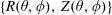
A smooth curve (green) for which the Frenet–Serret frame is discontinuous:
 $R(\unicode[STIX]{x1D719})=1+0.1\cos (3\unicode[STIX]{x1D719})$
,
$R(\unicode[STIX]{x1D719})=1+0.1\cos (3\unicode[STIX]{x1D719})$
,
 $z(\unicode[STIX]{x1D719})=0.1\sin (3\unicode[STIX]{x1D719})$
.
$z(\unicode[STIX]{x1D719})=0.1\sin (3\unicode[STIX]{x1D719})$
.
Our second motivation in this paper is to modify Garren & Boozer’s analysis to avoid the Frenet–Serret frame because this basis can be pathological in certain situations of interest. The Frenet–Serret frame is known to be problematic if there are any points of vanishing curvature: even smooth curves can have discontinuous Frenet–Serret basis vectors. For instance, for the curve defined by
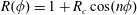 $R(\unicode[STIX]{x1D719})=1+R_{c}\cos (n\unicode[STIX]{x1D719})$
and
$R(\unicode[STIX]{x1D719})=1+R_{c}\cos (n\unicode[STIX]{x1D719})$
and
 $z(\unicode[STIX]{x1D719})=z_{s}\sin (n\unicode[STIX]{x1D719})$
, the curvature vanishes if
$z(\unicode[STIX]{x1D719})=z_{s}\sin (n\unicode[STIX]{x1D719})$
, the curvature vanishes if
 $R_{c}=1/(n^{2}+1)$
, and the Frenet basis is generally discontinuous at these points, as shown in figure 1. Where
$R_{c}=1/(n^{2}+1)$
, and the Frenet basis is generally discontinuous at these points, as shown in figure 1. Where
 $\unicode[STIX]{x1D705}=0$
, the torsion is generally not well defined. This situation of vanishing
$\unicode[STIX]{x1D705}=0$
, the torsion is generally not well defined. This situation of vanishing
 $\unicode[STIX]{x1D705}$
is of particular interest because it is necessary for a desirable
$\unicode[STIX]{x1D705}$
is of particular interest because it is necessary for a desirable
 $B(r,\unicode[STIX]{x1D703},\unicode[STIX]{x1D711})$
optimization: omnigenity with poloidally closed
$B(r,\unicode[STIX]{x1D703},\unicode[STIX]{x1D711})$
optimization: omnigenity with poloidally closed
 $B$
contours (Cary & Shasharina Reference Cary and Shasharina1997; Subbotin et al.
Reference Subbotin, Mikhailov, Shafranov, Isaev, Nührenberg, Nührenberg, Zille, Nemov, Kasilov and Kalyuzhnyj2006; Helander & Nührenberg Reference Helander and Nührenberg2009; Landreman & Catto Reference Landreman and Catto2012) (sometimes called ‘quasi-isodynamic’). In this optimization, which yields good particle confinement at the same time as vanishing bootstrap current (Helander & Nührenberg Reference Helander and Nührenberg2009), the maximum of
$B$
contours (Cary & Shasharina Reference Cary and Shasharina1997; Subbotin et al.
Reference Subbotin, Mikhailov, Shafranov, Isaev, Nührenberg, Nührenberg, Zille, Nemov, Kasilov and Kalyuzhnyj2006; Helander & Nührenberg Reference Helander and Nührenberg2009; Landreman & Catto Reference Landreman and Catto2012) (sometimes called ‘quasi-isodynamic’). In this optimization, which yields good particle confinement at the same time as vanishing bootstrap current (Helander & Nührenberg Reference Helander and Nührenberg2009), the maximum of
 $B$
on each
$B$
on each
 $r$
surface must be a constant-
$r$
surface must be a constant-
 $\unicode[STIX]{x1D711}$
curve, so
$\unicode[STIX]{x1D711}$
curve, so
 $\unicode[STIX]{x2202}B/\unicode[STIX]{x2202}\unicode[STIX]{x1D703}$
must vanish for all
$\unicode[STIX]{x2202}B/\unicode[STIX]{x2202}\unicode[STIX]{x1D703}$
must vanish for all
 $\unicode[STIX]{x1D703}$
at these
$\unicode[STIX]{x1D703}$
at these
 $\unicode[STIX]{x1D711}$
values. To see that this condition near the axis implies
$\unicode[STIX]{x1D711}$
values. To see that this condition near the axis implies
 $\unicode[STIX]{x1D705}=0$
, consider that the pressure gradient
$\unicode[STIX]{x1D705}=0$
, consider that the pressure gradient
 $\unicode[STIX]{x1D735}p$
vanishes on the magnetic axis, so it follows from the MHD equilibrium relation
$\unicode[STIX]{x1D735}p$
vanishes on the magnetic axis, so it follows from the MHD equilibrium relation
 $(\unicode[STIX]{x1D735}\times \boldsymbol{B})\times \boldsymbol{B}=0$
that
$(\unicode[STIX]{x1D735}\times \boldsymbol{B})\times \boldsymbol{B}=0$
that
 $$\begin{eqnarray}\unicode[STIX]{x1D735}_{\bot }B=\boldsymbol{B}\boldsymbol{\cdot }\unicode[STIX]{x1D735}(B^{-1}\boldsymbol{B})=B\unicode[STIX]{x1D705}\boldsymbol{n}.\end{eqnarray}$$
The condition
 $\unicode[STIX]{x2202}B/\unicode[STIX]{x2202}\unicode[STIX]{x1D703}$
on the maximum-
$\unicode[STIX]{x2202}B/\unicode[STIX]{x2202}\unicode[STIX]{x1D703}$
on the maximum-
 $B$
curves near the axis implies
$B$
curves near the axis implies
 $\unicode[STIX]{x1D735}_{\bot }B=0$
there, implying
$\unicode[STIX]{x1D735}_{\bot }B=0$
there, implying
 $\unicode[STIX]{x1D705}=0$
. While one would have to grapple with discontinuities and ill-defined torsion to apply the Frenet–Serret approach to construct omnigenous fields with poloidally closed
$\unicode[STIX]{x1D705}=0$
. While one would have to grapple with discontinuities and ill-defined torsion to apply the Frenet–Serret approach to construct omnigenous fields with poloidally closed
 $B$
contours, all quantities remain smooth in cylindrical coordinates. Construction of omnigenous magnetic fields will be considered in Part 3 of this series.
$B$
contours, all quantities remain smooth in cylindrical coordinates. Construction of omnigenous magnetic fields will be considered in Part 3 of this series.
The Frenet–Serret frame has also been used in another important stellarator calculation: Mercier’s result that rotational transform on the magnetic axis arises from a combination of axis torsion, rotating elongation and current density (Mercier Reference Mercier1964; Helander Reference Helander2014). This result was also derived by Garren & Boozer (Reference Garren and Boozer1991a ) as part of their quasi-symmetry analysis, as their equation (77). Just as Garren & Boozer’s quasi-symmetry equation acquires singularities if the axis curvature ever vanishes, so does Mercier’s expression for the rotational transform, as it includes torsion explicitly. As part of our analysis, we will re-derive Mercier’s result in cylindrical coordinates, resulting in an expression that does not become singular if the axis curvature vanishes.
The main content of this paper begins in § 2 with the calculation of the relationship between
 $B(r,\unicode[STIX]{x1D703},\unicode[STIX]{x1D711})$
and flux surface shape directly in cylindrical coordinates. The analogous results of the Garren–Boozer calculation in the Frenet–Serret frame are then reviewed in § 3. The transformation between the two coordinate systems is derived in § 4.1, and this transformation is used in the remainder of § 4 to prove that the cylindrical and Frenet–Serret equations are equivalent, when the latter are valid. Some reductions of the equations for the particular case of quasi-symmetry are discussed in § 5, and we will conclude in § 6.
$B(r,\unicode[STIX]{x1D703},\unicode[STIX]{x1D711})$
and flux surface shape directly in cylindrical coordinates. The analogous results of the Garren–Boozer calculation in the Frenet–Serret frame are then reviewed in § 3. The transformation between the two coordinate systems is derived in § 4.1, and this transformation is used in the remainder of § 4 to prove that the cylindrical and Frenet–Serret equations are equivalent, when the latter are valid. Some reductions of the equations for the particular case of quasi-symmetry are discussed in § 5, and we will conclude in § 6.
2 Direct calculation in cylindrical coordinates
We now present the calculation in which the field strength in Boozer coordinates is directly related to the magnetic surface shape in cylindrical coordinates. Aside from the fact that we describe the magnetic surface shapes in cylindrical coordinates rather than by the projections along the Frenet–Serret vectors, our approach is similar in structure to the one in Garren & Boozer (Reference Garren and Boozer1991a
). The covariant and contravariant expressions for
 $\boldsymbol{B}$
in Boozer coordinates are equated, giving three independent equations. The square of either expression for
$\boldsymbol{B}$
in Boozer coordinates are equated, giving three independent equations. The square of either expression for
 $\boldsymbol{B}$
gives an additional equation for
$\boldsymbol{B}$
gives an additional equation for
 $B$
. These four equations are then expanded in the distance
$B$
. These four equations are then expanded in the distance
 $r$
from the magnetic axis. Here we will carry out the expansion to sufficient order that the first-order quantities in
$r$
from the magnetic axis. Here we will carry out the expansion to sufficient order that the first-order quantities in
 $r$
are determined.
$r$
are determined.
2.1 Starting equations
In any straight-field-line coordinates, including Boozer coordinates, the magnetic field can be written
 $$\begin{eqnarray}\boldsymbol{B}=\unicode[STIX]{x1D735}\unicode[STIX]{x1D713}\times \unicode[STIX]{x1D735}\unicode[STIX]{x1D703}+\unicode[STIX]{x1D704}\unicode[STIX]{x1D735}\unicode[STIX]{x1D711}\times \unicode[STIX]{x1D735}\unicode[STIX]{x1D713},\end{eqnarray}$$
where
 $2\unicode[STIX]{x03C0}\unicode[STIX]{x1D713}$
is the toroidal flux,
$2\unicode[STIX]{x03C0}\unicode[STIX]{x1D713}$
is the toroidal flux,
 $\unicode[STIX]{x1D704}$
is the rotational transform and
$\unicode[STIX]{x1D704}$
is the rotational transform and
 $\unicode[STIX]{x1D703}$
and
$\unicode[STIX]{x1D703}$
and
 $\unicode[STIX]{x1D711}$
are the poloidal and toroidal angles. In the particular case of Boozer coordinates,
$\unicode[STIX]{x1D711}$
are the poloidal and toroidal angles. In the particular case of Boozer coordinates,
 $\boldsymbol{B}$
can also be written
$\boldsymbol{B}$
can also be written
 $$\begin{eqnarray}\boldsymbol{B}=\unicode[STIX]{x1D6FD}(\unicode[STIX]{x1D713},\unicode[STIX]{x1D703},\unicode[STIX]{x1D719})\unicode[STIX]{x1D735}\unicode[STIX]{x1D713}+I(\unicode[STIX]{x1D713})\unicode[STIX]{x1D735}\unicode[STIX]{x1D703}+G(\unicode[STIX]{x1D713})\unicode[STIX]{x1D735}\unicode[STIX]{x1D711}.\end{eqnarray}$$
Here
 $I(\unicode[STIX]{x1D713})$
is
$I(\unicode[STIX]{x1D713})$
is
 $\unicode[STIX]{x1D707}_{0}/(2\unicode[STIX]{x03C0})$
times the toroidal current enclosed by the flux surface, and
$\unicode[STIX]{x1D707}_{0}/(2\unicode[STIX]{x03C0})$
times the toroidal current enclosed by the flux surface, and
 $G(\unicode[STIX]{x1D713})$
is
$G(\unicode[STIX]{x1D713})$
is
 $\unicode[STIX]{x1D707}_{0}/(2\unicode[STIX]{x03C0})$
times the poloidal current outside the flux surface. The Boozer toroidal angle
$\unicode[STIX]{x1D707}_{0}/(2\unicode[STIX]{x03C0})$
times the poloidal current outside the flux surface. The Boozer toroidal angle
 $\unicode[STIX]{x1D711}$
differs from the cylindrical azimuthal angle
$\unicode[STIX]{x1D711}$
differs from the cylindrical azimuthal angle
 $\unicode[STIX]{x1D719}$
, and we will keep track of the difference, denoted
$\unicode[STIX]{x1D719}$
, and we will keep track of the difference, denoted
 $\unicode[STIX]{x1D708}$
:
$\unicode[STIX]{x1D708}$
:
 $$\begin{eqnarray}\unicode[STIX]{x1D711}=\unicode[STIX]{x1D719}+\unicode[STIX]{x1D708}.\end{eqnarray}$$
(By assuming this equation, our analysis will not pertain to certain unconventional configurations such as knots in which
 $\unicode[STIX]{x1D719}$
increases by an integer
$\unicode[STIX]{x1D719}$
increases by an integer
 ${>}1$
multiple of
${>}1$
multiple of
 $2\unicode[STIX]{x03C0}$
when
$2\unicode[STIX]{x03C0}$
when
 $\unicode[STIX]{x1D711}$
increases by
$\unicode[STIX]{x1D711}$
increases by
 $2\unicode[STIX]{x03C0}$
.) We will consider the independent variables to be
$2\unicode[STIX]{x03C0}$
.) We will consider the independent variables to be
 $(\unicode[STIX]{x1D713},\unicode[STIX]{x1D703},\unicode[STIX]{x1D719})$
. From the product of (2.1) and (2.2), the Jacobian of these coordinates is
$(\unicode[STIX]{x1D713},\unicode[STIX]{x1D703},\unicode[STIX]{x1D719})$
. From the product of (2.1) and (2.2), the Jacobian of these coordinates is
 $$\begin{eqnarray}\sqrt{g}=\frac{1}{\unicode[STIX]{x1D735}\unicode[STIX]{x1D713}\boldsymbol{\cdot }\unicode[STIX]{x1D735}\unicode[STIX]{x1D703}\times \unicode[STIX]{x1D735}\unicode[STIX]{x1D719}}=\left(1+\frac{\unicode[STIX]{x2202}\unicode[STIX]{x1D708}}{\unicode[STIX]{x2202}\unicode[STIX]{x1D719}}\right)\frac{G+\unicode[STIX]{x1D704}I}{B^{2}}.\end{eqnarray}$$
We will assume
 $\unicode[STIX]{x2202}\unicode[STIX]{x1D708}/\unicode[STIX]{x2202}\unicode[STIX]{x1D719}>-1$
so this Jacobian remains non-zero. Physically, this assumption means the direction of
$\unicode[STIX]{x2202}\unicode[STIX]{x1D708}/\unicode[STIX]{x2202}\unicode[STIX]{x1D719}>-1$
so this Jacobian remains non-zero. Physically, this assumption means the direction of
 $\boldsymbol{B}$
always points toward increasing
$\boldsymbol{B}$
always points toward increasing
 $\unicode[STIX]{x1D719}$
or always points towards decreasing
$\unicode[STIX]{x1D719}$
or always points towards decreasing
 $\unicode[STIX]{x1D719}$
, never reversing direction. This same assumption is made in the VMEC code (Hirshman & Whitson Reference Hirshman and Whitson1983), and it is not restrictive in practice.
$\unicode[STIX]{x1D719}$
, never reversing direction. This same assumption is made in the VMEC code (Hirshman & Whitson Reference Hirshman and Whitson1983), and it is not restrictive in practice.
Using the dual relations
 $$\begin{eqnarray}\frac{\unicode[STIX]{x2202}\boldsymbol{r}}{\unicode[STIX]{x2202}\unicode[STIX]{x1D713}}=\sqrt{g}\unicode[STIX]{x1D735}\unicode[STIX]{x1D703}\times \unicode[STIX]{x1D735}\unicode[STIX]{x1D719},\quad \unicode[STIX]{x1D735}\unicode[STIX]{x1D713}=\frac{1}{\sqrt{g}}\frac{\unicode[STIX]{x2202}\boldsymbol{r}}{\unicode[STIX]{x2202}\unicode[STIX]{x1D703}}\times \frac{\unicode[STIX]{x2202}\boldsymbol{r}}{\unicode[STIX]{x2202}\unicode[STIX]{x1D719}},\quad \text{and cyclic permutations},\end{eqnarray}$$
where
 $\boldsymbol{r}$
is the position vector, we can write (2.1) as
$\boldsymbol{r}$
is the position vector, we can write (2.1) as
 $$\begin{eqnarray}\boldsymbol{B}=\frac{B^{2}}{G+\unicode[STIX]{x1D704}I}\left[\left(1+\frac{\unicode[STIX]{x2202}\unicode[STIX]{x1D708}}{\unicode[STIX]{x2202}\unicode[STIX]{x1D719}}\right)^{-1}\left(1-\unicode[STIX]{x1D704}\frac{\unicode[STIX]{x2202}\unicode[STIX]{x1D708}}{\unicode[STIX]{x2202}\unicode[STIX]{x1D703}}\right)\frac{\unicode[STIX]{x2202}\boldsymbol{r}}{\unicode[STIX]{x2202}\unicode[STIX]{x1D719}}+\unicode[STIX]{x1D704}\frac{\unicode[STIX]{x2202}\boldsymbol{r}}{\unicode[STIX]{x2202}\unicode[STIX]{x1D703}}\right],\end{eqnarray}$$
and write (2.2) as
 $$\begin{eqnarray}\displaystyle \boldsymbol{B} & = & \displaystyle \frac{B^{2}}{G+\unicode[STIX]{x1D704}I}\left[\left(1+\frac{\unicode[STIX]{x2202}\unicode[STIX]{x1D708}}{\unicode[STIX]{x2202}\unicode[STIX]{x1D719}}\right)^{-1}\left(\unicode[STIX]{x1D6FD}+G\frac{\unicode[STIX]{x2202}\unicode[STIX]{x1D708}}{\unicode[STIX]{x2202}\unicode[STIX]{x1D713}}\right)\frac{\unicode[STIX]{x2202}\boldsymbol{r}}{\unicode[STIX]{x2202}\unicode[STIX]{x1D703}}\times \frac{\unicode[STIX]{x2202}\boldsymbol{r}}{\unicode[STIX]{x2202}\unicode[STIX]{x1D719}}\right.\nonumber\\ \displaystyle & & \displaystyle +\,\left.\left(1+\frac{\unicode[STIX]{x2202}\unicode[STIX]{x1D708}}{\unicode[STIX]{x2202}\unicode[STIX]{x1D719}}\right)^{-1}\left(I+G\frac{\unicode[STIX]{x2202}\unicode[STIX]{x1D708}}{\unicode[STIX]{x2202}\unicode[STIX]{x1D703}}\right)\frac{\unicode[STIX]{x2202}\boldsymbol{r}}{\unicode[STIX]{x2202}\unicode[STIX]{x1D719}}\times \frac{\unicode[STIX]{x2202}\boldsymbol{r}}{\unicode[STIX]{x2202}\unicode[STIX]{x1D713}}+G\frac{\unicode[STIX]{x2202}\boldsymbol{r}}{\unicode[STIX]{x2202}\unicode[STIX]{x1D713}}\times \frac{\unicode[STIX]{x2202}\boldsymbol{r}}{\unicode[STIX]{x2202}\unicode[STIX]{x1D703}}\right].\end{eqnarray}$$
The derivatives of
 $\boldsymbol{r}(\unicode[STIX]{x1D713},\unicode[STIX]{x1D703},\unicode[STIX]{x1D719})=R\boldsymbol{e}_{R}+z\boldsymbol{e}_{z}$
can be evaluated using
$\boldsymbol{r}(\unicode[STIX]{x1D713},\unicode[STIX]{x1D703},\unicode[STIX]{x1D719})=R\boldsymbol{e}_{R}+z\boldsymbol{e}_{z}$
can be evaluated using
 $\text{d}\boldsymbol{e}_{R}/\text{d}\unicode[STIX]{x1D719}=\boldsymbol{e}_{\unicode[STIX]{x1D719}}$
, where
$\text{d}\boldsymbol{e}_{R}/\text{d}\unicode[STIX]{x1D719}=\boldsymbol{e}_{\unicode[STIX]{x1D719}}$
, where
 $(\boldsymbol{e}_{R},\boldsymbol{e}_{\unicode[STIX]{x1D719}},\boldsymbol{e}_{z})$
are cylindrical unit basis vectors. Equating the three cylindrical components of (2.6) and (2.7), we obtain
$(\boldsymbol{e}_{R},\boldsymbol{e}_{\unicode[STIX]{x1D719}},\boldsymbol{e}_{z})$
are cylindrical unit basis vectors. Equating the three cylindrical components of (2.6) and (2.7), we obtain
 $$\begin{eqnarray}\frac{r\bar{B}}{R}\left[\left(1-\unicode[STIX]{x1D704}\frac{\unicode[STIX]{x2202}\unicode[STIX]{x1D708}}{\unicode[STIX]{x2202}\unicode[STIX]{x1D703}}\right)\frac{\unicode[STIX]{x2202}R}{\unicode[STIX]{x2202}\unicode[STIX]{x1D719}}+\unicode[STIX]{x1D704}\left(1+\frac{\unicode[STIX]{x2202}\unicode[STIX]{x1D708}}{\unicode[STIX]{x2202}\unicode[STIX]{x1D719}}\right)\frac{\unicode[STIX]{x2202}R}{\unicode[STIX]{x2202}\unicode[STIX]{x1D703}}\right]=\left(I+G\frac{\unicode[STIX]{x2202}\unicode[STIX]{x1D708}}{\unicode[STIX]{x2202}\unicode[STIX]{x1D703}}\right)\frac{\unicode[STIX]{x2202}z}{\unicode[STIX]{x2202}r}-\left(\unicode[STIX]{x1D6FD}r\bar{B}+G\frac{\unicode[STIX]{x2202}\unicode[STIX]{x1D708}}{\unicode[STIX]{x2202}r}\right)\frac{\unicode[STIX]{x2202}z}{\unicode[STIX]{x2202}\unicode[STIX]{x1D703}},\end{eqnarray}$$
 $$\begin{eqnarray}\displaystyle & & \displaystyle \frac{r\bar{B}}{GR}\left\{\left(1-\unicode[STIX]{x1D704}\frac{\unicode[STIX]{x2202}\unicode[STIX]{x1D708}}{\unicode[STIX]{x2202}\unicode[STIX]{x1D703}}\right)\left[R^{2}+\left(\frac{\unicode[STIX]{x2202}R}{\unicode[STIX]{x2202}\unicode[STIX]{x1D719}}\right)^{2}+\left(\frac{\unicode[STIX]{x2202}z}{\unicode[STIX]{x2202}\unicode[STIX]{x1D719}}\right)^{2}\right]+\unicode[STIX]{x1D704}\left(1+\frac{\unicode[STIX]{x2202}\unicode[STIX]{x1D708}}{\unicode[STIX]{x2202}\unicode[STIX]{x1D719}}\right)\left(\frac{\unicode[STIX]{x2202}R}{\unicode[STIX]{x2202}\unicode[STIX]{x1D703}}\frac{\unicode[STIX]{x2202}R}{\unicode[STIX]{x2202}\unicode[STIX]{x1D719}}+\frac{\unicode[STIX]{x2202}z}{\unicode[STIX]{x2202}\unicode[STIX]{x1D703}}\frac{\unicode[STIX]{x2202}z}{\unicode[STIX]{x2202}\unicode[STIX]{x1D719}}\right)\right\}\nonumber\\ \displaystyle & & \displaystyle \qquad =\left(\frac{\unicode[STIX]{x2202}z}{\unicode[STIX]{x2202}r}\frac{\unicode[STIX]{x2202}R}{\unicode[STIX]{x2202}\unicode[STIX]{x1D703}}-\frac{\unicode[STIX]{x2202}R}{\unicode[STIX]{x2202}r}\frac{\unicode[STIX]{x2202}z}{\unicode[STIX]{x2202}\unicode[STIX]{x1D703}}\right)\left(1+\frac{\unicode[STIX]{x2202}\unicode[STIX]{x1D708}}{\unicode[STIX]{x2202}\unicode[STIX]{x1D719}}\right),\end{eqnarray}$$
 $$\begin{eqnarray}\frac{r\bar{B}}{R}\left[\left(1-\unicode[STIX]{x1D704}\frac{\unicode[STIX]{x2202}\unicode[STIX]{x1D708}}{\unicode[STIX]{x2202}\unicode[STIX]{x1D703}}\right)\frac{\unicode[STIX]{x2202}z}{\unicode[STIX]{x2202}\unicode[STIX]{x1D719}}+\unicode[STIX]{x1D704}\left(1+\frac{\unicode[STIX]{x2202}\unicode[STIX]{x1D708}}{\unicode[STIX]{x2202}\unicode[STIX]{x1D719}}\right)\frac{\unicode[STIX]{x2202}z}{\unicode[STIX]{x2202}\unicode[STIX]{x1D703}}\right]=\left(\unicode[STIX]{x1D6FD}r\bar{B}+G\frac{\unicode[STIX]{x2202}\unicode[STIX]{x1D708}}{\unicode[STIX]{x2202}r}\right)\frac{\unicode[STIX]{x2202}R}{\unicode[STIX]{x2202}\unicode[STIX]{x1D703}}-\left(I+G\frac{\unicode[STIX]{x2202}\unicode[STIX]{x1D708}}{\unicode[STIX]{x2202}\unicode[STIX]{x1D703}}\right)\frac{\unicode[STIX]{x2202}R}{\unicode[STIX]{x2202}r}.\end{eqnarray}$$
To get (2.9) we have added (2.8) times
 $\unicode[STIX]{x2202}R/\unicode[STIX]{x2202}\unicode[STIX]{x1D719}$
and (2.10) times
$\unicode[STIX]{x2202}R/\unicode[STIX]{x2202}\unicode[STIX]{x1D719}$
and (2.10) times
 $\unicode[STIX]{x2202}z/\unicode[STIX]{x2202}\unicode[STIX]{x1D719}$
to the
$\unicode[STIX]{x2202}z/\unicode[STIX]{x2202}\unicode[STIX]{x1D719}$
to the
 $\boldsymbol{e}_{\unicode[STIX]{x1D719}}$
components. In these expressions, we have changed the flux surface label coordinate from
$\boldsymbol{e}_{\unicode[STIX]{x1D719}}$
components. In these expressions, we have changed the flux surface label coordinate from
 $\unicode[STIX]{x1D713}$
to the effective minor radius
$\unicode[STIX]{x1D713}$
to the effective minor radius
 $r(\unicode[STIX]{x1D713})$
defined by
$r(\unicode[STIX]{x1D713})$
defined by
 $2\unicode[STIX]{x03C0}\unicode[STIX]{x1D713}=\unicode[STIX]{x03C0}r^{2}\bar{B}$
, where
$2\unicode[STIX]{x03C0}\unicode[STIX]{x1D713}=\unicode[STIX]{x03C0}r^{2}\bar{B}$
, where
 $\bar{B}$
is an arbitrary reference magnitude of magnetic field. (Since
$\bar{B}$
is an arbitrary reference magnitude of magnetic field. (Since
 $\unicode[STIX]{x1D713}$
can be negative,
$\unicode[STIX]{x1D713}$
can be negative,
 $\bar{B}$
may be negative.) Also, a relation for
$\bar{B}$
may be negative.) Also, a relation for
 $B$
can be obtained by squaring (2.6):
$B$
can be obtained by squaring (2.6):
 $$\begin{eqnarray}\displaystyle \frac{(G+\unicode[STIX]{x1D704}I)^{2}}{B^{2}}\left(1+\frac{\unicode[STIX]{x2202}\unicode[STIX]{x1D708}}{\unicode[STIX]{x2202}\unicode[STIX]{x1D719}}\right)^{2} & = & \displaystyle \left[\left(1-\unicode[STIX]{x1D704}\frac{\unicode[STIX]{x2202}\unicode[STIX]{x1D708}}{\unicode[STIX]{x2202}\unicode[STIX]{x1D703}}\right)\frac{\unicode[STIX]{x2202}R}{\unicode[STIX]{x2202}\unicode[STIX]{x1D719}}+\unicode[STIX]{x1D704}\left(1+\frac{\unicode[STIX]{x2202}\unicode[STIX]{x1D708}}{\unicode[STIX]{x2202}\unicode[STIX]{x1D719}}\right)\frac{\unicode[STIX]{x2202}R}{\unicode[STIX]{x2202}\unicode[STIX]{x1D703}}\right]^{2}+\left(1-\unicode[STIX]{x1D704}\frac{\unicode[STIX]{x2202}\unicode[STIX]{x1D708}}{\unicode[STIX]{x2202}\unicode[STIX]{x1D703}}\right)^{2}R^{2}\nonumber\\ \displaystyle & & \displaystyle +\,\left[\left(1-\unicode[STIX]{x1D704}\frac{\unicode[STIX]{x2202}\unicode[STIX]{x1D708}}{\unicode[STIX]{x2202}\unicode[STIX]{x1D703}}\right)\frac{\unicode[STIX]{x2202}z}{\unicode[STIX]{x2202}\unicode[STIX]{x1D719}}+\unicode[STIX]{x1D704}\left(1+\frac{\unicode[STIX]{x2202}\unicode[STIX]{x1D708}}{\unicode[STIX]{x2202}\unicode[STIX]{x1D719}}\right)\frac{\unicode[STIX]{x2202}z}{\unicode[STIX]{x2202}\unicode[STIX]{x1D703}}\right]^{2}.\end{eqnarray}$$
Equations (2.8)–(2.11) are the basis of the remainder of the analysis, in which these equations will be systematically expanded.
2.2 Expansion about the magnetic axis
We take the magnetic axis to be described by its cylindrical coordinates
 $R_{0}(\unicode[STIX]{x1D719})$
and
$R_{0}(\unicode[STIX]{x1D719})$
and
 $z_{0}(\unicode[STIX]{x1D719})$
. Regularity considerations near the axis imply we can write the cylindrical coordinate
$z_{0}(\unicode[STIX]{x1D719})$
. Regularity considerations near the axis imply we can write the cylindrical coordinate
 $R(r,\unicode[STIX]{x1D703},\unicode[STIX]{x1D719})$
for a general point near the axis in the form of an expansion
$R(r,\unicode[STIX]{x1D703},\unicode[STIX]{x1D719})$
for a general point near the axis in the form of an expansion
 $$\begin{eqnarray}R(r,\unicode[STIX]{x1D703},\unicode[STIX]{x1D719})=R_{0}(\unicode[STIX]{x1D719})+rR_{1}(\unicode[STIX]{x1D703},\unicode[STIX]{x1D719})+r^{2}R_{2}(\unicode[STIX]{x1D703},\unicode[STIX]{x1D719})+\cdots \,,\end{eqnarray}$$
where
 $$\begin{eqnarray}\displaystyle & \displaystyle R_{1}(\unicode[STIX]{x1D703},\unicode[STIX]{x1D719})=R_{1c}(\unicode[STIX]{x1D719})\cos \unicode[STIX]{x1D703}+R_{1s}(\unicode[STIX]{x1D719})\sin \unicode[STIX]{x1D703}, & \displaystyle\end{eqnarray}$$
 $$\begin{eqnarray}\displaystyle & \displaystyle R_{2}(\unicode[STIX]{x1D703},\unicode[STIX]{x1D719})=R_{2c}(\unicode[STIX]{x1D719})\cos 2\unicode[STIX]{x1D703}+R_{2s}(\unicode[STIX]{x1D719})\sin 2\unicode[STIX]{x1D703}+R_{20}(\unicode[STIX]{x1D719}). & \displaystyle\end{eqnarray}$$
Expansions of the same form are made for
 $z$
,
$z$
,
 $\unicode[STIX]{x1D708}$
and
$\unicode[STIX]{x1D708}$
and
 $B$
:
$B$
:
 $$\begin{eqnarray}\displaystyle \left.\begin{array}{@{}rcl@{}}z\ & =\ & z_{0}(\unicode[STIX]{x1D719})+r[z_{1c}(\unicode[STIX]{x1D719})\cos \unicode[STIX]{x1D703}+z_{1s}(\unicode[STIX]{x1D719})\sin \unicode[STIX]{x1D703}]\\ \ & \ & +\,r^{2}[z_{20}(\unicode[STIX]{x1D719})+z_{2c}(\unicode[STIX]{x1D719})\cos 2\unicode[STIX]{x1D703}+z_{2s}(\unicode[STIX]{x1D719})\sin 2\unicode[STIX]{x1D703}]+\cdots \\ \unicode[STIX]{x1D708}\ & =\ & \unicode[STIX]{x1D708}_{0}(\unicode[STIX]{x1D719})+r[\unicode[STIX]{x1D708}_{1c}(\unicode[STIX]{x1D719})\cos \unicode[STIX]{x1D703}+\unicode[STIX]{x1D708}_{1s}(\unicode[STIX]{x1D719})\sin \unicode[STIX]{x1D703}]\\ \ & \ & +\,r^{2}[\unicode[STIX]{x1D708}_{20}(\unicode[STIX]{x1D719})+\unicode[STIX]{x1D708}_{2c}(\unicode[STIX]{x1D719})\cos 2\unicode[STIX]{x1D703}+\unicode[STIX]{x1D708}_{2s}(\unicode[STIX]{x1D719})\sin 2\unicode[STIX]{x1D703}]+\cdots \\ B\ & =\ & B_{0}(\unicode[STIX]{x1D719})+r[B_{1c}(\unicode[STIX]{x1D719})\cos \unicode[STIX]{x1D703}+B_{1s}(\unicode[STIX]{x1D719})\sin \unicode[STIX]{x1D703}]\\ \ & \ & +\,r^{2}[B_{20}(\unicode[STIX]{x1D719})+B_{2c}(\unicode[STIX]{x1D719})\cos 2\unicode[STIX]{x1D703}+B_{2s}(\unicode[STIX]{x1D719})\sin 2\unicode[STIX]{x1D703}]+\cdots \,.\end{array}\right\} & & \displaystyle\end{eqnarray}$$
These expansions are justified in appendix A. We also have
 $$\begin{eqnarray}\displaystyle & \displaystyle G(r)=G_{0}+r^{2}G_{2}+\cdots \,, & \displaystyle\end{eqnarray}$$
 $$\begin{eqnarray}\displaystyle & \displaystyle I(r)=r^{2}I_{2}+\cdots \,, & \displaystyle\end{eqnarray}$$
 $$\begin{eqnarray}\displaystyle & \displaystyle \unicode[STIX]{x1D6FD}(r,\unicode[STIX]{x1D703},\unicode[STIX]{x1D719})=\unicode[STIX]{x1D6FD}_{0}(\unicode[STIX]{x1D719})+r\unicode[STIX]{x1D6FD}_{1}(\unicode[STIX]{x1D703},\unicode[STIX]{x1D719})+\cdots \,, & \displaystyle\end{eqnarray}$$
 $$\begin{eqnarray}\displaystyle & \displaystyle \unicode[STIX]{x1D704}(r)=\unicode[STIX]{x1D704}_{0}+\cdots \,. & \displaystyle\end{eqnarray}$$
Using these expansions, we proceed to systematically consider the terms of each order in (2.8)–(2.11).
2.3 Magnitude of
 $B$
: zeroth order
$B$
: zeroth order

We first consider the
 $O(r^{0})$
terms in (2.11). These terms give
$O(r^{0})$
terms in (2.11). These terms give
 $$\begin{eqnarray}\unicode[STIX]{x1D708}_{0}^{\prime }=-1+s_{G}\ell ^{\prime }B_{0}/G_{0},\end{eqnarray}$$
where
 $s_{G}=\pm 1$
, primes denote
$s_{G}=\pm 1$
, primes denote
 $\text{d}/\text{d}\unicode[STIX]{x1D719}$
, and
$\text{d}/\text{d}\unicode[STIX]{x1D719}$
, and
 $\ell ^{\prime }>0$
is the differential length of the magnetic axis:
$\ell ^{\prime }>0$
is the differential length of the magnetic axis:
 $$\begin{eqnarray}\ell ^{\prime }=\sqrt{R_{0}^{2}+(R_{0}^{\prime })^{2}+(z_{0}^{\prime })^{2}}.\end{eqnarray}$$
Integrating (2.20) in
 $\unicode[STIX]{x1D719}$
,
$\unicode[STIX]{x1D719}$
,
 $$\begin{eqnarray}G_{0}=\frac{s_{G}}{2\unicode[STIX]{x03C0}}\int _{0}^{2\unicode[STIX]{x03C0}}\text{d}\unicode[STIX]{x1D719}\;B_{0}\ell ^{\prime }.\end{eqnarray}$$
Thus,
 $s_{G}$
is the sign of
$s_{G}$
is the sign of
 $G_{0}$
,
$G_{0}$
,
 $+1$
if
$+1$
if
 $\boldsymbol{B}$
points in the direction of increasing
$\boldsymbol{B}$
points in the direction of increasing
 $\unicode[STIX]{x1D719}$
and
$\unicode[STIX]{x1D719}$
and
 $-1$
otherwise. Equations (2.20)–(2.22) allow us to eliminate
$-1$
otherwise. Equations (2.20)–(2.22) allow us to eliminate
 $\unicode[STIX]{x1D708}_{0}$
and
$\unicode[STIX]{x1D708}_{0}$
and
 $G_{0}$
in favour of
$G_{0}$
in favour of
 $R_{0}$
,
$R_{0}$
,
 $z_{0}$
and
$z_{0}$
and
 $B_{0}$
.
$B_{0}$
.
2.4 Equating representations of the field: first order
Next, the leading-order terms in the
 $r$
expansion of (2.9) are
$r$
expansion of (2.9) are
 $O(r^{1})$
, giving
$O(r^{1})$
, giving
 $$\begin{eqnarray}\frac{\bar{B}}{G_{0}R_{0}}(\ell ^{\prime })^{2}=\left(R_{1s}z_{1c}-R_{1c}z_{1s}\right)(1+\unicode[STIX]{x1D708}_{0}^{\prime }).\end{eqnarray}$$
We can eliminate
 $\unicode[STIX]{x1D708}_{0}$
in this equation using (2.20) to obtain
$\unicode[STIX]{x1D708}_{0}$
in this equation using (2.20) to obtain
 $$\begin{eqnarray}\frac{s_{G}\bar{B}\ell ^{\prime }}{R_{0}B_{0}}=R_{1s}z_{1c}-R_{1c}z_{1s}.\end{eqnarray}$$
This equation, which is analogous to (53) in Garren & Boozer (Reference Garren and Boozer1991a
), expresses the fact that the toroidal flux within the magnetic surface
 $r$
should be
$r$
should be
 $2\unicode[STIX]{x03C0}\unicode[STIX]{x1D713}=\unicode[STIX]{x03C0}r^{2}\bar{B}$
. To see this, consider that the toroidal field on the magnetic axis is
$2\unicode[STIX]{x03C0}\unicode[STIX]{x1D713}=\unicode[STIX]{x03C0}r^{2}\bar{B}$
. To see this, consider that the toroidal field on the magnetic axis is
 $\boldsymbol{B}\boldsymbol{\cdot }\boldsymbol{e}_{\unicode[STIX]{x1D719}}=s_{G}B_{0}\boldsymbol{t}\boldsymbol{\cdot }\boldsymbol{e}_{\unicode[STIX]{x1D719}}=B_{0}R_{0}/(s_{G}\ell ^{\prime })$
, and as shown in appendix B, the area of the flux surface in the constant-
$\boldsymbol{B}\boldsymbol{\cdot }\boldsymbol{e}_{\unicode[STIX]{x1D719}}=s_{G}B_{0}\boldsymbol{t}\boldsymbol{\cdot }\boldsymbol{e}_{\unicode[STIX]{x1D719}}=B_{0}R_{0}/(s_{G}\ell ^{\prime })$
, and as shown in appendix B, the area of the flux surface in the constant-
 $\unicode[STIX]{x1D719}$
plane is
$\unicode[STIX]{x1D719}$
plane is
 $\unicode[STIX]{x03C0}r^{2}$
times the right-hand side of (2.24).
$\unicode[STIX]{x03C0}r^{2}$
times the right-hand side of (2.24).
Similarly, the leading terms in (2.8) and (2.10) are
 $O(r^{1})$
and give
$O(r^{1})$
and give
 $$\begin{eqnarray}\displaystyle & \displaystyle \frac{\bar{B}R_{0}^{\prime }}{G_{0}R_{0}}=\unicode[STIX]{x1D708}_{1s}z_{1c}-\unicode[STIX]{x1D708}_{1c}z_{1s}, & \displaystyle\end{eqnarray}$$
 $$\begin{eqnarray}\displaystyle & \displaystyle \frac{\bar{B}z_{0}^{\prime }}{G_{0}R_{0}}=\unicode[STIX]{x1D708}_{1c}R_{1s}-\unicode[STIX]{x1D708}_{1s}R_{1c}. & \displaystyle\end{eqnarray}$$
Solving for
 $\unicode[STIX]{x1D708}_{1c}$
and
$\unicode[STIX]{x1D708}_{1c}$
and
 $\unicode[STIX]{x1D708}_{1s}$
and applying (2.24), we find
$\unicode[STIX]{x1D708}_{1s}$
and applying (2.24), we find
 $$\begin{eqnarray}\unicode[STIX]{x1D708}_{1}=\frac{B_{0}}{|G_{0}|\ell ^{\prime }}(R_{1}R_{0}^{\prime }+z_{1}z_{0}^{\prime }).\end{eqnarray}$$
2.5 Magnitude of
$B$
: first order

Another pair of equations is obtained from the
 $O(r^{1})$
terms in (2.11). These terms can be found by applying
$O(r^{1})$
terms in (2.11). These terms can be found by applying
 $\unicode[STIX]{x2202}/\unicode[STIX]{x2202}r$
to (2.11) and evaluating the result at
$\unicode[STIX]{x2202}/\unicode[STIX]{x2202}r$
to (2.11) and evaluating the result at
 $r\rightarrow 0$
. We find
$r\rightarrow 0$
. We find
 $$\begin{eqnarray}\displaystyle & & \displaystyle -\frac{G_{0}^{2}B_{1}}{B_{0}^{3}}(1+\unicode[STIX]{x1D708}_{0}^{\prime })^{2}+\frac{G_{0}^{2}}{B_{0}^{2}}(1+\unicode[STIX]{x1D708}_{0}^{\prime })\frac{\unicode[STIX]{x2202}\unicode[STIX]{x1D708}_{1}}{\unicode[STIX]{x2202}\unicode[STIX]{x1D719}}\nonumber\\ \displaystyle & & \displaystyle \quad =R_{0}^{\prime }\left[-\unicode[STIX]{x1D704}_{0}\frac{\unicode[STIX]{x2202}\unicode[STIX]{x1D708}_{1}}{\unicode[STIX]{x2202}\unicode[STIX]{x1D703}}R_{0}^{\prime }+\frac{\unicode[STIX]{x2202}R_{1}}{\unicode[STIX]{x2202}\unicode[STIX]{x1D719}}+\unicode[STIX]{x1D704}_{0}(1+\unicode[STIX]{x1D708}_{0}^{\prime })\frac{\unicode[STIX]{x2202}R_{1}}{\unicode[STIX]{x2202}\unicode[STIX]{x1D703}}\right]+R_{0}R_{1}-\unicode[STIX]{x1D704}_{0}\frac{\unicode[STIX]{x2202}\unicode[STIX]{x1D708}_{1}}{\unicode[STIX]{x2202}\unicode[STIX]{x1D703}}R_{0}^{2}\nonumber\\ \displaystyle & & \displaystyle \qquad +\,z_{0}^{\prime }\left[-\unicode[STIX]{x1D704}_{0}\frac{\unicode[STIX]{x2202}\unicode[STIX]{x1D708}_{1}}{\unicode[STIX]{x2202}\unicode[STIX]{x1D703}}z_{0}^{\prime }+\frac{\unicode[STIX]{x2202}z_{1}}{\unicode[STIX]{x2202}\unicode[STIX]{x1D719}}+\unicode[STIX]{x1D704}_{0}(1+\unicode[STIX]{x1D708}_{0}^{\prime })\frac{\unicode[STIX]{x2202}z_{1}}{\unicode[STIX]{x2202}\unicode[STIX]{x1D703}}\right].\end{eqnarray}$$
In this equation, the terms that include a factor of
 $\unicode[STIX]{x1D704}_{0}$
can be written
$\unicode[STIX]{x1D704}_{0}$
can be written
 $$\begin{eqnarray}\unicode[STIX]{x1D704}_{0}\frac{\unicode[STIX]{x2202}}{\unicode[STIX]{x2202}\unicode[STIX]{x1D703}}[-(\ell ^{\prime })^{2}\unicode[STIX]{x1D708}_{1}+(1+\unicode[STIX]{x1D708}_{0}^{\prime })(R_{1}R_{0}^{\prime }+z_{1}z_{0}^{\prime })],\end{eqnarray}$$
which can be seen to vanish in light of (2.27) and (2.20). Eliminating
 $\unicode[STIX]{x1D708}_{0}$
and
$\unicode[STIX]{x1D708}_{0}$
and
 $\unicode[STIX]{x1D708}_{1}$
in the remaining terms using (2.20) and (2.27), one finds
$\unicode[STIX]{x1D708}_{1}$
in the remaining terms using (2.20) and (2.27), one finds
 $$\begin{eqnarray}B_{1}/B_{0}=K_{R}R_{1}+K_{z}z_{1},\end{eqnarray}$$
where
 $$\begin{eqnarray}\displaystyle & \displaystyle K_{R}=-(\ell ^{\prime })^{-4}(R_{0}R_{0}^{\prime }+R_{0}^{\prime }R_{0}^{\prime \prime }+z_{0}^{\prime }z_{0}^{\prime \prime })R_{0}^{\prime }+(\ell ^{\prime })^{-2}(R_{0}^{\prime \prime }-R_{0}+R_{0}^{\prime }B_{0}^{\prime }/B_{0}), & \displaystyle\end{eqnarray}$$
 $$\begin{eqnarray}\displaystyle & \displaystyle K_{z}=-(\ell ^{\prime })^{-4}(R_{0}R_{0}^{\prime }+R_{0}^{\prime }R_{0}^{\prime \prime }+z_{0}^{\prime }z_{0}^{\prime \prime })z_{0}^{\prime }+(\ell ^{\prime })^{-2}(z_{0}^{\prime \prime }+z_{0}^{\prime }B_{0}^{\prime }/B_{0}). & \displaystyle\end{eqnarray}$$
Noting from the first line of (1.1) that
 $\unicode[STIX]{x1D705}\boldsymbol{n}\ell ^{\prime }=\boldsymbol{t}^{\prime }=[(\ell ^{\prime })^{-1}\boldsymbol{r}_{0}^{\prime }]^{\prime }$
, and evaluating the result in cylindrical coordinates, it can be seen that equivalent expressions to (2.31)–(2.32) are
$\unicode[STIX]{x1D705}\boldsymbol{n}\ell ^{\prime }=\boldsymbol{t}^{\prime }=[(\ell ^{\prime })^{-1}\boldsymbol{r}_{0}^{\prime }]^{\prime }$
, and evaluating the result in cylindrical coordinates, it can be seen that equivalent expressions to (2.31)–(2.32) are
 $$\begin{eqnarray}K_{R}=\unicode[STIX]{x1D705}\boldsymbol{n}\boldsymbol{\cdot }\boldsymbol{e}_{R}+(\ell ^{\prime })^{-2}R_{0}^{\prime }B_{0}^{\prime }/B_{0},\quad K_{z}=\unicode[STIX]{x1D705}\boldsymbol{n}\boldsymbol{\cdot }\boldsymbol{e}_{z}+(\ell ^{\prime })^{-2}z_{0}^{\prime }B_{0}^{\prime }/B_{0}.\end{eqnarray}$$
Note that the
 $\sin \unicode[STIX]{x1D703}$
and
$\sin \unicode[STIX]{x1D703}$
and
 $\cos \unicode[STIX]{x1D703}$
components of
$\cos \unicode[STIX]{x1D703}$
components of
 $B_{1}$
,
$B_{1}$
,
 $R_{1}$
and
$R_{1}$
and
 $z_{1}$
each satisfy (2.30) separately. Equations (2.30)–(2.32) are analogous to (70) in Garren & Boozer (Reference Garren and Boozer1991a
). These equations reflect (1.2). In the limit of a circular magnetic axis,
$z_{1}$
each satisfy (2.30) separately. Equations (2.30)–(2.32) are analogous to (70) in Garren & Boozer (Reference Garren and Boozer1991a
). These equations reflect (1.2). In the limit of a circular magnetic axis,
 $R_{0}^{\prime }=0$
and
$R_{0}^{\prime }=0$
and
 $z_{0}^{\prime }=0$
, equation (2.30)–(2.32) reduce to
$z_{0}^{\prime }=0$
, equation (2.30)–(2.32) reduce to
 $B_{1}/B_{0}=-R_{1}/R_{0}$
, reflecting the expected
$B_{1}/B_{0}=-R_{1}/R_{0}$
, reflecting the expected
 $B\propto 1/R$
variation.
$B\propto 1/R$
variation.
2.6 Equating representations of the field: second order
The highest-order terms in the
 $r$
expansion we will consider are the
$r$
expansion we will consider are the
 $O(r^{2})$
terms in (2.8)–(2.10). The expressions at this order become rather lengthy and so details are left to appendix C. At
$O(r^{2})$
terms in (2.8)–(2.10). The expressions at this order become rather lengthy and so details are left to appendix C. At
 $O(r^{2})$
, the three equations (2.8)–(2.10) each have a
$O(r^{2})$
, the three equations (2.8)–(2.10) each have a
 $\sin \unicode[STIX]{x1D703}$
and
$\sin \unicode[STIX]{x1D703}$
and
 $\cos \unicode[STIX]{x1D703}$
component, so there are six independent equations. Although nine second-order quantities (
$\cos \unicode[STIX]{x1D703}$
component, so there are six independent equations. Although nine second-order quantities (
 $R_{2s}$
,
$R_{2s}$
,
 $R_{2c}$
,
$R_{2c}$
,
 $R_{20}$
and similar
$R_{20}$
and similar
 $\unicode[STIX]{x1D708}$
and
$\unicode[STIX]{x1D708}$
and
 $z$
terms) appear, they only enter through five linearly independent combinations. Therefore the second-order quantities can be annihilated by forming a certain linear combination of the six equations, equation (C 10). What remains is an equation relating zeroth- and first-order quantities:
$z$
terms) appear, they only enter through five linearly independent combinations. Therefore the second-order quantities can be annihilated by forming a certain linear combination of the six equations, equation (C 10). What remains is an equation relating zeroth- and first-order quantities:
 $$\begin{eqnarray}\unicode[STIX]{x1D704}_{0}V-T=0,\end{eqnarray}$$
where
 $$\begin{eqnarray}\displaystyle T & = & \displaystyle \frac{|G_{0}|}{(\ell ^{\prime })^{3}B_{0}}\left[R_{0}^{2}(R_{1c}R_{1s}^{\prime }-R_{1s}R_{1c}^{\prime }+z_{1c}z_{1s}^{\prime }-z_{1s}z_{1c}^{\prime })\right.\nonumber\\ \displaystyle & & \displaystyle +\,(R_{1c}z_{1s}-R_{1s}z_{1c})(R_{0}^{\prime }z_{0}^{\prime \prime }+2R_{0}z_{0}^{\prime }-z_{0}^{\prime }R_{0}^{\prime \prime })\nonumber\\ \displaystyle & & \displaystyle +\,(z_{1c}z_{1s}^{\prime }-z_{1s}z_{1c}^{\prime })(R_{0}^{\prime })^{2}+(R_{1c}R_{1s}^{\prime }-R_{1s}R_{1c}^{\prime })(z_{0}^{\prime })^{2}\nonumber\\ \displaystyle & & \displaystyle +\,\left.(R_{1s}z_{1c}^{\prime }-z_{1c}R_{1s}^{\prime }+z_{1s}R_{1c}^{\prime }-R_{1c}z_{1s}^{\prime })R_{0}^{\prime }z_{0}^{\prime }\right]+\frac{2G_{0}I_{2}}{B_{0}^{2}}\end{eqnarray}$$
and
 $$\begin{eqnarray}\displaystyle V & = & \displaystyle \frac{1}{(\ell ^{\prime })^{2}}\left[R_{0}^{2}(R_{1c}^{2}+R_{1s}^{2}+z_{1c}^{2}+z_{1s}^{2})+\left(R_{0}^{\prime }\right)^{2}(z_{1c}^{2}+z_{1s}^{2})\right.\nonumber\\ \displaystyle & & \displaystyle \left.-\,2R_{0}^{\prime }z_{0}^{\prime }(R_{1c}z_{1c}+R_{1s}z_{1s})+(z_{0}^{\prime })^{2}(R_{1c}^{2}+R_{1s}^{2})\right].\end{eqnarray}$$
Our (2.34)–(2.36) play an analogous role to (63) and (67) in Garren & Boozer (Reference Garren and Boozer1991a
). Note that (2.34) can be integrated to give
 $\unicode[STIX]{x1D704}_{0}=(\oint w\,\text{d}\unicode[STIX]{x1D719})^{-1}\oint (wT/V)\,\text{d}\unicode[STIX]{x1D719}$
for any
$\unicode[STIX]{x1D704}_{0}=(\oint w\,\text{d}\unicode[STIX]{x1D719})^{-1}\oint (wT/V)\,\text{d}\unicode[STIX]{x1D719}$
for any
 $w(\unicode[STIX]{x1D719})$
, analogous to Garren & Boozer’s (77). Encoded in these equations is the classic result by Mercier (Reference Mercier1964), Helander (Reference Helander2014): rotational transform on the magnetic axis arises due to axis torsion, rotating elongation and toroidal current. Indeed, in Part 2 we will compute
$w(\unicode[STIX]{x1D719})$
, analogous to Garren & Boozer’s (77). Encoded in these equations is the classic result by Mercier (Reference Mercier1964), Helander (Reference Helander2014): rotational transform on the magnetic axis arises due to axis torsion, rotating elongation and toroidal current. Indeed, in Part 2 we will compute
 $\unicode[STIX]{x1D704}_{0}$
numerically by solving (2.34)–(2.36) or its Frenet–Serret analogue. The toroidal current contribution to
$\unicode[STIX]{x1D704}_{0}$
numerically by solving (2.34)–(2.36) or its Frenet–Serret analogue. The toroidal current contribution to
 $\unicode[STIX]{x1D704}_{0}$
is the
$\unicode[STIX]{x1D704}_{0}$
is the
 $I_{2}$
term in
$I_{2}$
term in
 $T$
, while the axis torsion and rotating elongation contributions are evidently contained in the remaining terms. Interestingly, while the torsion in Mercier’s expression involves the third derivative of the axis shape, the highest derivative of the axis shape appearing in (2.34)–(2.36) is the second. If there are any points where the axis curvature vanishes, the torsion becomes ill defined, so Mercier’s expression for
$T$
, while the axis torsion and rotating elongation contributions are evidently contained in the remaining terms. Interestingly, while the torsion in Mercier’s expression involves the third derivative of the axis shape, the highest derivative of the axis shape appearing in (2.34)–(2.36) is the second. If there are any points where the axis curvature vanishes, the torsion becomes ill defined, so Mercier’s expression for
 $\unicode[STIX]{x1D704}$
(which explicitly depends on
$\unicode[STIX]{x1D704}$
(which explicitly depends on
 $\unicode[STIX]{x1D70F}$
) becomes awkward; equation (2.34) has no such problem.
$\unicode[STIX]{x1D70F}$
) becomes awkward; equation (2.34) has no such problem.
Another perspective on rotational transform and torsion in cases with vanishing curvature (without effects of elongation) has been discussed by Pfefferlé et al. (Reference Pfefferlé, Gunderson, Hudson and Noakes2018).
3 Frenet–Serret approach
The analogous calculation using the Frenet–Serret frame is clearly explained in Garren & Boozer (Reference Garren and Boozer1991a ,Reference Garren and Boozer b ), so we will not repeat it here, only quote the main results. The position vector is written
 $$\begin{eqnarray}\boldsymbol{r}(r,\unicode[STIX]{x1D703},\unicode[STIX]{x1D711})=\boldsymbol{r}_{0}(\unicode[STIX]{x1D711})+X(r,\unicode[STIX]{x1D703},\unicode[STIX]{x1D711})\boldsymbol{n}(\unicode[STIX]{x1D711})+Y(r,\unicode[STIX]{x1D703},\unicode[STIX]{x1D711})\boldsymbol{b}(\unicode[STIX]{x1D711})+Z(r,\unicode[STIX]{x1D703},\unicode[STIX]{x1D711})\boldsymbol{t}(\unicode[STIX]{x1D711}),\end{eqnarray}$$
where
 $\boldsymbol{r}_{0}$
,
$\boldsymbol{r}_{0}$
,
 $\boldsymbol{n}$
,
$\boldsymbol{n}$
,
 $\boldsymbol{b}$
and
$\boldsymbol{b}$
and
 $\boldsymbol{t}$
refer to the magnetic axis. The quantities
$\boldsymbol{t}$
refer to the magnetic axis. The quantities
 $X$
,
$X$
,
 $Y$
and
$Y$
and
 $Z$
are expanded similarly to (2.12)–(2.14) but with
$Z$
are expanded similarly to (2.12)–(2.14) but with
 $\unicode[STIX]{x1D719}\rightarrow \unicode[STIX]{x1D711}$
:
$\unicode[STIX]{x1D719}\rightarrow \unicode[STIX]{x1D711}$
:
 $$\begin{eqnarray}X(r,\unicode[STIX]{x1D703},\unicode[STIX]{x1D711})=rX_{1}(\unicode[STIX]{x1D703},\unicode[STIX]{x1D711})+r^{2}X_{2}(\unicode[STIX]{x1D703},\unicode[STIX]{x1D711})+\cdots\end{eqnarray}$$
where regularity requires
 $$\begin{eqnarray}\displaystyle & \displaystyle X_{1}(\unicode[STIX]{x1D703},\unicode[STIX]{x1D711})=X_{1c}(\unicode[STIX]{x1D711})\cos \unicode[STIX]{x1D703}+X_{1s}(\unicode[STIX]{x1D711})\sin \unicode[STIX]{x1D703}, & \displaystyle\end{eqnarray}$$
 $$\begin{eqnarray}\displaystyle & \displaystyle X_{2}(\unicode[STIX]{x1D703},\unicode[STIX]{x1D711})=X_{2c}(\unicode[STIX]{x1D711})\cos 2\unicode[STIX]{x1D703}+X_{2s}(\unicode[STIX]{x1D711})\sin 2\unicode[STIX]{x1D703}+X_{20}(\unicode[STIX]{x1D711}), & \displaystyle\end{eqnarray}$$
and analogous expansions are made for
 $Y$
and
$Y$
and
 $Z$
. The expansion of
$Z$
. The expansion of
 $B$
is written in terms of
$B$
is written in terms of
 $\unicode[STIX]{x1D711}$
rather than
$\unicode[STIX]{x1D711}$
rather than
 $\unicode[STIX]{x1D719}$
, so
$\unicode[STIX]{x1D719}$
, so
 $$\begin{eqnarray}B(r,\unicode[STIX]{x1D719},\unicode[STIX]{x1D711})=\hat{B}_{0}(\unicode[STIX]{x1D711})+r\hat{B}_{1}(\unicode[STIX]{x1D703},\unicode[STIX]{x1D711})+\cdots \,,\end{eqnarray}$$
where
 $\hat{B}_{1}(\unicode[STIX]{x1D703},\unicode[STIX]{x1D711})=\hat{B}_{1s}(\unicode[STIX]{x1D711})\sin \unicode[STIX]{x1D703}+\hat{B}_{1c}(\unicode[STIX]{x1D711})\cos \unicode[STIX]{x1D703}$
.
$\hat{B}_{1}(\unicode[STIX]{x1D703},\unicode[STIX]{x1D711})=\hat{B}_{1s}(\unicode[STIX]{x1D711})\sin \unicode[STIX]{x1D703}+\hat{B}_{1c}(\unicode[STIX]{x1D711})\cos \unicode[STIX]{x1D703}$
.
Instead of (2.20), one obtains
 $G_{0}=s_{G}B_{0}\,\text{d}\ell /\text{d}\unicode[STIX]{x1D711}$
. Instead of (2.24), one finds
$G_{0}=s_{G}B_{0}\,\text{d}\ell /\text{d}\unicode[STIX]{x1D711}$
. Instead of (2.24), one finds
 $Z_{1}=0$
and
$Z_{1}=0$
and
 $$\begin{eqnarray}X_{1c}Y_{1s}-X_{1s}Y_{1c}=s_{G}\bar{B}/B_{0}.\end{eqnarray}$$
Noting from appendix B that the left-hand side of this equation is the cross-sectional area of the flux surface in a plane perpendicular to the on-axis
 $\boldsymbol{B}$
, equation (3.6) represents the fact that the toroidal flux inside the flux surface is
$\boldsymbol{B}$
, equation (3.6) represents the fact that the toroidal flux inside the flux surface is
 $\unicode[STIX]{x03C0}r^{2}\bar{B}$
. Instead of (2.30), one finds
$\unicode[STIX]{x03C0}r^{2}\bar{B}$
. Instead of (2.30), one finds
 $$\begin{eqnarray}\hat{B}_{1}/\hat{B}_{0}=\unicode[STIX]{x1D705}X_{1},\end{eqnarray}$$
where this equation holds separately for
 $\sin \unicode[STIX]{x1D703}$
and
$\sin \unicode[STIX]{x1D703}$
and
 $\cos \unicode[STIX]{x1D703}$
components. Instead of (2.34)–(2.36), Garren & Boozer obtain
$\cos \unicode[STIX]{x1D703}$
components. Instead of (2.34)–(2.36), Garren & Boozer obtain
 $$\begin{eqnarray}\unicode[STIX]{x1D704}_{0}V^{FS}-T^{FS}=0,\end{eqnarray}$$
where
 $$\begin{eqnarray}V^{FS}=X_{1s}^{2}+X_{1c}^{2}+Y_{1s}^{2}+Y_{1c}^{2}\end{eqnarray}$$
and
 $$\begin{eqnarray}T^{FS}=X_{1c}\frac{\text{d}X_{1s}}{\text{d}\unicode[STIX]{x1D711}}-X_{1s}\frac{\text{d}X_{1c}}{\text{d}\unicode[STIX]{x1D711}}+Y_{1c}\frac{\text{d}Y_{1s}}{\text{d}\unicode[STIX]{x1D711}}-Y_{1s}\frac{\text{d}Y_{1c}}{\text{d}\unicode[STIX]{x1D711}}+2\left(\frac{I_{2}}{\bar{B}}-\unicode[STIX]{x1D70F}\right)\frac{G_{0}\bar{B}}{B_{0}^{2}}.\end{eqnarray}$$
These equations correspond to (63) in Garren & Boozer (Reference Garren and Boozer1991a
), but with an extra
 $I_{2}$
term since a vacuum field was assumed in that work. The fact that a
$I_{2}$
term since a vacuum field was assumed in that work. The fact that a
 $2$
appears in the
$2$
appears in the
 $\unicode[STIX]{x1D70F}$
term here whereas a 4 appears in Garren & Boozer (Reference Garren and Boozer1991a
) is due to the normalization used in the latter, and
$\unicode[STIX]{x1D70F}$
term here whereas a 4 appears in Garren & Boozer (Reference Garren and Boozer1991a
) is due to the normalization used in the latter, and
 $\unicode[STIX]{x1D70F}$
enters with the opposite sign due to the opposite sign convention for torsion.
$\unicode[STIX]{x1D70F}$
enters with the opposite sign due to the opposite sign convention for torsion.
Combining the above equations to eliminate unknowns, the system can be reduced to a single equation. To this end, we introduce a variable
 $\unicode[STIX]{x1D70E}(\unicode[STIX]{x1D711})$
related to the flux surface shape, defined by
$\unicode[STIX]{x1D70E}(\unicode[STIX]{x1D711})$
related to the flux surface shape, defined by
 $$\begin{eqnarray}s_{G}\bar{B}\unicode[STIX]{x1D705}\unicode[STIX]{x1D70E}=\hat{B}_{1s}Y_{1s}+\hat{B}_{1c}Y_{1c}.\end{eqnarray}$$
From this definition and (3.6)–(3.7),
 $$\begin{eqnarray}\left.\begin{array}{@{}c@{}}\displaystyle Y_{1s}=\frac{s_{G}\bar{B}\unicode[STIX]{x1D705}}{\hat{B}_{1s}^{2}+\hat{B}_{1c}^{2}}(\hat{B}_{1c}+\hat{B}_{1s}\unicode[STIX]{x1D70E}),\\ \displaystyle Y_{1c}=\frac{s_{G}\bar{B}\unicode[STIX]{x1D705}}{\hat{B}_{1s}^{2}+\hat{B}_{1c}^{2}}(-\hat{B}_{1s}+\hat{B}_{1c}\unicode[STIX]{x1D70E}).\end{array}\right\}\end{eqnarray}$$
Substituting these results and (3.7) into (3.8), we obtain
 $$\begin{eqnarray}\displaystyle & & \displaystyle \frac{\text{d}\unicode[STIX]{x1D70E}}{\text{d}\unicode[STIX]{x1D711}}+\left[\frac{(\hat{B}_{1s}^{2}+\hat{B}_{1c}^{2})^{2}}{B_{0}^{2}\bar{B}^{2}\unicode[STIX]{x1D705}^{4}}+1+\unicode[STIX]{x1D70E}^{2}\right]\left[\unicode[STIX]{x1D704}_{0}+\frac{1}{\hat{B}_{1s}^{2}+\hat{B}_{1c}^{2}}\left(\hat{B}_{1s}\frac{\text{d}\hat{B}_{1c}}{\text{d}\unicode[STIX]{x1D711}}-\hat{B}_{1c}\frac{\text{d}\hat{B}_{1s}}{\text{d}\unicode[STIX]{x1D711}}\right)\right]\nonumber\\ \displaystyle & & \displaystyle \qquad -\,2\left(\frac{I_{2}}{\bar{B}}-\unicode[STIX]{x1D70F}\right)\frac{G_{0}(\hat{B}_{1s}^{2}+\hat{B}_{1c}^{2})}{\bar{B}B_{0}^{2}\unicode[STIX]{x1D705}^{2}}=0.\end{eqnarray}$$
Considering
 $\unicode[STIX]{x1D705}$
,
$\unicode[STIX]{x1D705}$
,
 $\unicode[STIX]{x1D70F}$
,
$\unicode[STIX]{x1D70F}$
,
 $I_{2}$
,
$I_{2}$
,
 $B_{0}$
,
$B_{0}$
,
 $\hat{B}_{1s}$
and
$\hat{B}_{1s}$
and
 $\hat{B}_{1c}$
to be known, this result is a first-order nonlinear ordinary differential equation for
$\hat{B}_{1c}$
to be known, this result is a first-order nonlinear ordinary differential equation for
 $\unicode[STIX]{x1D70E}$
. Once
$\unicode[STIX]{x1D70E}$
. Once
 $\unicode[STIX]{x1D70E}$
is obtained,
$\unicode[STIX]{x1D70E}$
is obtained,
 $Y_{1s}$
and
$Y_{1s}$
and
 $Y_{1c}$
can be found from (3.12), and
$Y_{1c}$
can be found from (3.12), and
 $X_{1s}$
and
$X_{1s}$
and
 $X_{1c}$
are known from (3.7), so the flux surface shape can be reconstructed from (3.1).
$X_{1c}$
are known from (3.7), so the flux surface shape can be reconstructed from (3.1).
4 Equivalence of the two approaches
4.1 Relating representations of the surface shape
Let us now prove that if the curvature of the magnetic axis does not vanish, the Frenet–Serret approach and the direct calculation in cylindrical coordinates are equivalent, as they should be. To begin, we must relate
 $X_{1}$
and
$X_{1}$
and
 $Y_{1}$
to
$Y_{1}$
to
 $R_{1}$
and
$R_{1}$
and
 $z_{1}$
. This can be done by equating the position vector in the two approaches, expanding (3.1) using
$z_{1}$
. This can be done by equating the position vector in the two approaches, expanding (3.1) using
 $\unicode[STIX]{x1D711}(r,\unicode[STIX]{x1D703},\unicode[STIX]{x1D719})=\unicode[STIX]{x1D711}_{0}(\unicode[STIX]{x1D719})+r\unicode[STIX]{x1D708}_{1}(\unicode[STIX]{x1D703},\unicode[STIX]{x1D719})+O(r^{2})$
where
$\unicode[STIX]{x1D711}(r,\unicode[STIX]{x1D703},\unicode[STIX]{x1D719})=\unicode[STIX]{x1D711}_{0}(\unicode[STIX]{x1D719})+r\unicode[STIX]{x1D708}_{1}(\unicode[STIX]{x1D703},\unicode[STIX]{x1D719})+O(r^{2})$
where
 $\unicode[STIX]{x1D711}_{0}(\unicode[STIX]{x1D719})=\unicode[STIX]{x1D719}+\unicode[STIX]{x1D708}_{0}(\unicode[STIX]{x1D719})$
:
$\unicode[STIX]{x1D711}_{0}(\unicode[STIX]{x1D719})=\unicode[STIX]{x1D719}+\unicode[STIX]{x1D708}_{0}(\unicode[STIX]{x1D719})$
:
 $$\begin{eqnarray}\displaystyle & & \displaystyle [R_{0}(\unicode[STIX]{x1D719})+rR_{1}(\unicode[STIX]{x1D703},\unicode[STIX]{x1D719})]\boldsymbol{e}_{R}(\unicode[STIX]{x1D719})+[z_{0}(\unicode[STIX]{x1D719})+rz_{1}(\unicode[STIX]{x1D703},\unicode[STIX]{x1D719})]\boldsymbol{e}_{z}+O(r^{2})\nonumber\\ \displaystyle & & \displaystyle \quad =\boldsymbol{r}_{0}(\unicode[STIX]{x1D711}_{0})+r\unicode[STIX]{x1D708}_{1}(\unicode[STIX]{x1D703},\unicode[STIX]{x1D719})\,\text{d}\boldsymbol{r}_{0}/\text{d}\unicode[STIX]{x1D711}_{0}+rX_{1}(\unicode[STIX]{x1D703},\unicode[STIX]{x1D711}_{0})\boldsymbol{n}(\unicode[STIX]{x1D711}_{0})+rY_{1}(\unicode[STIX]{x1D703},\unicode[STIX]{x1D711}_{0})\boldsymbol{b}(\unicode[STIX]{x1D711}_{0})+O(r^{2}).\qquad\end{eqnarray}$$
Equating the
 $O(r^{0})$
terms gives
$O(r^{0})$
terms gives
 $\boldsymbol{r}_{0}(\unicode[STIX]{x1D711}_{0})=R_{0}(\unicode[STIX]{x1D719})\boldsymbol{e}_{R}(\unicode[STIX]{x1D719})+z_{0}(\unicode[STIX]{x1D719})\boldsymbol{e}_{z}$
. Then applying
$\boldsymbol{r}_{0}(\unicode[STIX]{x1D711}_{0})=R_{0}(\unicode[STIX]{x1D719})\boldsymbol{e}_{R}(\unicode[STIX]{x1D719})+z_{0}(\unicode[STIX]{x1D719})\boldsymbol{e}_{z}$
. Then applying
 $\boldsymbol{n}(\unicode[STIX]{x1D711}_{0})\boldsymbol{\cdot }(\ldots )$
and
$\boldsymbol{n}(\unicode[STIX]{x1D711}_{0})\boldsymbol{\cdot }(\ldots )$
and
 $\boldsymbol{b}(\unicode[STIX]{x1D711}_{0})\boldsymbol{\cdot }(\ldots )$
to the
$\boldsymbol{b}(\unicode[STIX]{x1D711}_{0})\boldsymbol{\cdot }(\ldots )$
to the
 $O(r)$
terms in (4.1), we obtain two equations that can be represented
$O(r)$
terms in (4.1), we obtain two equations that can be represented
 $$\begin{eqnarray}\left(\begin{array}{@{}c@{}}X_{1}\\ Y_{1}\end{array}\right)=\left(\begin{array}{@{}cc@{}}n_{R} & n_{z}\\ b_{R} & b_{z}\end{array}\right)\left(\begin{array}{@{}c@{}}R_{1}\\ z_{1}\end{array}\right).\end{eqnarray}$$
Here and for the rest of this section,
 $n_{R}=\boldsymbol{n}(\unicode[STIX]{x1D711}_{0})\boldsymbol{\cdot }\boldsymbol{e}_{R}(\unicode[STIX]{x1D719})$
,
$n_{R}=\boldsymbol{n}(\unicode[STIX]{x1D711}_{0})\boldsymbol{\cdot }\boldsymbol{e}_{R}(\unicode[STIX]{x1D719})$
,
 $b_{R}=\boldsymbol{b}(\unicode[STIX]{x1D711}_{0})\boldsymbol{\cdot }\boldsymbol{e}_{R}(\unicode[STIX]{x1D719})$
, analogous expressions hold for
$b_{R}=\boldsymbol{b}(\unicode[STIX]{x1D711}_{0})\boldsymbol{\cdot }\boldsymbol{e}_{R}(\unicode[STIX]{x1D719})$
, analogous expressions hold for
 $n_{z}$
and
$n_{z}$
and
 $b_{z}$
and
$b_{z}$
and
 $X_{1}$
and
$X_{1}$
and
 $Y_{1}$
are understood to be evaluated at
$Y_{1}$
are understood to be evaluated at
 $\unicode[STIX]{x1D711}_{0}$
. (The
$\unicode[STIX]{x1D711}_{0}$
. (The
 $\boldsymbol{t}(\unicode[STIX]{x1D711}_{0})\boldsymbol{\cdot }(\ldots )$
component of (4.1) yields (2.27).)
$\boldsymbol{t}(\unicode[STIX]{x1D711}_{0})\boldsymbol{\cdot }(\ldots )$
component of (4.1) yields (2.27).)
Noting the components of the tangent vector in cylindrical coordinates,
 $$\begin{eqnarray}t_{R}=\boldsymbol{t}\boldsymbol{\cdot }\boldsymbol{e}_{R}=R_{0}^{\prime }/\ell ^{\prime },\quad t_{\unicode[STIX]{x1D719}}=\boldsymbol{t}\boldsymbol{\cdot }\boldsymbol{e}_{\unicode[STIX]{x1D719}}=R_{0}/\ell ^{\prime },\quad t_{z}=\boldsymbol{t}\boldsymbol{\cdot }\boldsymbol{e}_{z}=z_{0}^{\prime }/\ell ^{\prime },\end{eqnarray}$$
the determinant of the matrix in (4.2) is
 $$\begin{eqnarray}n_{R}b_{z}-b_{R}n_{z}=-\boldsymbol{n}\times \boldsymbol{b}\boldsymbol{\cdot }\boldsymbol{e}_{\unicode[STIX]{x1D719}}=-\boldsymbol{t}\boldsymbol{\cdot }\boldsymbol{e}_{\unicode[STIX]{x1D719}}=-R_{0}/\ell ^{\prime }.\end{eqnarray}$$
Hence the inverse transformation is
 $$\begin{eqnarray}\left(\begin{array}{@{}c@{}}R_{1}\\ z_{1}\end{array}\right)=\frac{\ell ^{\prime }}{R_{0}}\left(\begin{array}{@{}cc@{}}-b_{z} & n_{z}\\ b_{R} & -n_{R}\end{array}\right)\left(\begin{array}{@{}c@{}}X_{1}\\ Y_{1}\end{array}\right).\end{eqnarray}$$
This relation enables the solution of the quasi-symmetry equations in the Frenet–Serret basis to be mapped to cylindrical coordinates. Note that by applying (4.5) and (4.4) to (2.24), we obtain (3.6), and so these equations from the Frenet–Serret and cylindrical coordinates analyses are consistent.
4.2 Equivalence of the
$B_{1}$
equations

Next let us show that (2.30) and (3.7) are equivalent. Expanding (3.5) about
 $\unicode[STIX]{x1D711}\approx \unicode[STIX]{x1D711}_{0}$
, and equating the result to the
$\unicode[STIX]{x1D711}\approx \unicode[STIX]{x1D711}_{0}$
, and equating the result to the
 $B$
analogue of (2.12), we obtain
$B$
analogue of (2.12), we obtain
 $$\begin{eqnarray}B_{0}(\unicode[STIX]{x1D719})+rB_{1}(\unicode[STIX]{x1D703},\unicode[STIX]{x1D719})+O(r^{2})=\hat{B}_{0}(\unicode[STIX]{x1D711}_{0})+r\unicode[STIX]{x1D708}_{1}(\unicode[STIX]{x1D703},\unicode[STIX]{x1D719})\,\text{d}\hat{B}_{0}/\text{d}\unicode[STIX]{x1D711}_{0}+r\hat{B}_{1}(\unicode[STIX]{x1D703},\unicode[STIX]{x1D711}_{0})+O(r^{2}).\end{eqnarray}$$
The
 $O(r^{0})$
terms give
$O(r^{0})$
terms give
 $B_{0}(\unicode[STIX]{x1D719})=\hat{B}_{0}(\unicode[STIX]{x1D711}_{0})$
, which upon differentiation gives
$B_{0}(\unicode[STIX]{x1D719})=\hat{B}_{0}(\unicode[STIX]{x1D711}_{0})$
, which upon differentiation gives
 $$\begin{eqnarray}B_{0}^{\prime }(\unicode[STIX]{x1D719})=[1+\unicode[STIX]{x1D708}_{0}^{\prime }(\unicode[STIX]{x1D719})]\,\text{d}\hat{B}_{0}/\text{d}\unicode[STIX]{x1D711}_{0}.\end{eqnarray}$$
Combining this result with (2.20), (2.27) and the
 $O(r^{1})$
terms of (4.6), we find
$O(r^{1})$
terms of (4.6), we find
 $$\begin{eqnarray}\hat{B}_{1}(\unicode[STIX]{x1D703},\unicode[STIX]{x1D711}_{0})=B_{1}-B_{0}^{\prime }(\ell ^{\prime })^{-2}(R_{0}^{\prime }R_{1}+z_{0}^{\prime }z_{1}).\end{eqnarray}$$
Then using the top row of (4.2), (3.7) and (2.30) are equivalent. Note that using (4.8), (2.30) can be written in terms of
 $\hat{B}_{1}$
rather than
$\hat{B}_{1}$
rather than
 $B_{1}$
, yielding a relation between the flux surface shape in cylindrical coordinates and the field strength in Boozer coordinates:
$B_{1}$
, yielding a relation between the flux surface shape in cylindrical coordinates and the field strength in Boozer coordinates:
 $$\begin{eqnarray}\hat{B}_{1}(\unicode[STIX]{x1D703},\unicode[STIX]{x1D711}_{0})/\hat{B}_{0}(\unicode[STIX]{x1D711}_{0})=(n_{R}R_{1}+n_{z}z_{1})\unicode[STIX]{x1D705}.\end{eqnarray}$$
4.3 Equivalence of the
$\unicode[STIX]{x1D704}_{0}$
equations

Finally, let us show that equations (2.34)–(2.36), which determine
 $\unicode[STIX]{x1D704}_{0}$
in cylindrical coordinates, can be independently derived from the analogous Frenet–Serret equations (3.8)–(3.10) by applying the transformation (4.2). We first note the following relations between components of the normal and binormal vectors:
$\unicode[STIX]{x1D704}_{0}$
in cylindrical coordinates, can be independently derived from the analogous Frenet–Serret equations (3.8)–(3.10) by applying the transformation (4.2). We first note the following relations between components of the normal and binormal vectors:
 $$\begin{eqnarray}\left.\begin{array}{@{}l@{}}\displaystyle n_{R}^{2}+b_{R}^{2}=[(\boldsymbol{t}\boldsymbol{t}+\boldsymbol{n}\boldsymbol{n}+\boldsymbol{b}\boldsymbol{b})\boldsymbol{\cdot }\boldsymbol{e}_{R}]^{2}-t_{R}^{2}=1-t_{R}^{2}=\frac{R_{0}^{2}+(z_{0}^{\prime })^{2}}{(\ell ^{\prime })^{2}},\\ \displaystyle n_{z}^{2}+b_{z}^{2}=[(\boldsymbol{t}\boldsymbol{t}+\boldsymbol{n}\boldsymbol{n}+\boldsymbol{b}\boldsymbol{b})\boldsymbol{\cdot }\boldsymbol{e}_{z}]^{2}-t_{z}^{2}=1-t_{z}^{2}=\frac{R_{0}^{2}+(R_{0}^{\prime })^{2}}{(\ell ^{\prime })^{2}},\\ \displaystyle n_{R}n_{z}+b_{R}b_{z}=\boldsymbol{e}_{R}\boldsymbol{\cdot }(\boldsymbol{t}\boldsymbol{t}+\boldsymbol{n}\boldsymbol{n}+\boldsymbol{b}\boldsymbol{b})\boldsymbol{\cdot }\boldsymbol{e}_{z}-t_{R}t_{z}=\boldsymbol{e}_{R}\boldsymbol{\cdot }\boldsymbol{e}_{z}-t_{R}t_{z}=-t_{R}t_{z}=-R_{0}^{\prime }z_{0}^{\prime }/(\ell ^{\prime })^{2}.\end{array}\right\}\end{eqnarray}$$
Using these results and (4.5), then
 $$\begin{eqnarray}X_{1s}^{2}+Y_{1s}^{2}=(\ell ^{\prime })^{-2}[R_{0}^{2}(R_{1s}^{2}+z_{1s}^{2})+(z_{0}^{\prime })^{2}R_{1s}^{2}-2R_{0}^{\prime }z_{0}^{\prime }R_{1s}z_{1s}+(R_{0}^{\prime })^{2}z_{1s}^{2}].\end{eqnarray}$$
An analogous expression holds for the subscript-
 $1c$
(
$1c$
(
 $\cos \unicode[STIX]{x1D703}$
) terms. Thus, it can be seen that
$\cos \unicode[STIX]{x1D703}$
) terms. Thus, it can be seen that
 $V^{FS}=V$
.
$V^{FS}=V$
.
It remains to show
 $T^{FS}=T$
. To show this equivalence we first apply (4.2) and then (4.10) to the first four terms of
$T^{FS}=T$
. To show this equivalence we first apply (4.2) and then (4.10) to the first four terms of
 $T^{FS}$
, giving
$T^{FS}$
, giving
 $$\begin{eqnarray}\displaystyle T^{FS} & = & \displaystyle \frac{|G_{0}|}{B_{0}(\ell ^{\prime })^{3}}\left[R_{0}^{2}(R_{1c}R_{1s}^{\prime }-R_{1s}R_{1c}^{\prime }+z_{1c}z_{1s}^{\prime }-z_{1s}z_{1c}^{\prime })\right.\nonumber\\ \displaystyle & & \displaystyle +\,(z_{1c}z_{1s}^{\prime }-z_{1s}z_{1c}^{\prime })(R_{0}^{\prime })^{2}+(R_{1c}R_{1s}^{\prime }-R_{1s}R_{1c}^{\prime })(z_{0}^{\prime })^{2}\nonumber\\ \displaystyle & & \displaystyle +\,\left.(R_{1s}z_{1c}^{\prime }-z_{1c}R_{1s}^{\prime }+z_{1s}R_{1c}^{\prime }-R_{1c}z_{1s}^{\prime })R_{0}^{\prime }z_{0}^{\prime }\right]+\frac{2I_{2}G_{0}}{B_{0}^{2}}+\hat{T},\end{eqnarray}$$
where
 $$\begin{eqnarray}\hat{T}=\frac{|G_{0}|}{B_{0}\ell ^{\prime }}(R_{1s}z_{1c}-R_{1c}z_{1s})(n_{z}n_{R}^{\prime }-n_{R}n_{z}^{\prime }+b_{z}b_{R}^{\prime }-b_{R}b_{z}^{\prime })-2\unicode[STIX]{x1D70F}\frac{G_{0}\bar{B}}{B_{0}^{2}}.\end{eqnarray}$$
In the last term of (4.13),
 $\bar{B}$
is eliminated using (2.24). Applying the last two lines of (1.1),
$\bar{B}$
is eliminated using (2.24). Applying the last two lines of (1.1),
 $$\begin{eqnarray}n_{z}n_{R}^{\prime }-n_{R}n_{z}^{\prime }+b_{z}b_{R}^{\prime }-b_{R}b_{z}^{\prime }=2\unicode[STIX]{x1D70F}R_{0}+(n_{R}t_{z}-n_{z}t_{R})\ell ^{\prime }\unicode[STIX]{x1D705}+n_{z}n_{\unicode[STIX]{x1D719}}+b_{z}b_{\unicode[STIX]{x1D719}},\end{eqnarray}$$
where we have used
 $n_{z}b_{R}-b_{z}n_{R}=t_{\unicode[STIX]{x1D719}}=R_{0}/\ell ^{\prime }$
. Applying
$n_{z}b_{R}-b_{z}n_{R}=t_{\unicode[STIX]{x1D719}}=R_{0}/\ell ^{\prime }$
. Applying
 $$\begin{eqnarray}n_{z}n_{\unicode[STIX]{x1D719}}+b_{z}b_{\unicode[STIX]{x1D719}}=\boldsymbol{e}_{z}\boldsymbol{\cdot }(\boldsymbol{t}\boldsymbol{t}+\boldsymbol{n}\boldsymbol{n}+\boldsymbol{b}\boldsymbol{b})\boldsymbol{\cdot }\boldsymbol{e}_{\unicode[STIX]{x1D719}}-t_{z}t_{\unicode[STIX]{x1D719}}=-t_{z}t_{\unicode[STIX]{x1D719}}=-R_{0}z_{0}^{\prime }/(\ell ^{\prime })^{2}\end{eqnarray}$$
and
 $$\begin{eqnarray}(n_{z}t_{R}-n_{R}t_{z})\unicode[STIX]{x1D705}=t_{R}\boldsymbol{e}_{z}\boldsymbol{\cdot }\frac{\text{d}\boldsymbol{t}}{\text{d}\ell }-t_{z}\boldsymbol{e}_{R}\boldsymbol{\cdot }\frac{\text{d}\boldsymbol{t}}{\text{d}\ell }=\frac{R_{0}z_{0}^{\prime }+R_{0}^{\prime }z_{0}^{\prime \prime }-R_{0}^{\prime \prime }z_{0}^{\prime }}{(\ell ^{\prime })^{3}},\end{eqnarray}$$
we find
 $$\begin{eqnarray}\hat{T}=\frac{|G_{0}|}{B_{0}(\ell ^{\prime })^{3}}(R_{1c}z_{1s}-R_{1s}z_{1c})(R_{0}^{\prime }z_{0}^{\prime \prime }+2R_{0}z_{0}^{\prime }-z_{0}^{\prime }R_{0}^{\prime \prime }).\end{eqnarray}$$
Thus,
 $T^{FS}=T$
as desired. This concludes the proof that whenever the curvature of the magnetic axis does not vanish, so the Frenet–Serret approach is free of singularities, all the equations derived directly in cylindrical coordinates in § 2 are equivalent to the analogous equations derived in the Frenet–Serret frame by Garren & Boozer (Reference Garren and Boozer1991a
).
$T^{FS}=T$
as desired. This concludes the proof that whenever the curvature of the magnetic axis does not vanish, so the Frenet–Serret approach is free of singularities, all the equations derived directly in cylindrical coordinates in § 2 are equivalent to the analogous equations derived in the Frenet–Serret frame by Garren & Boozer (Reference Garren and Boozer1991a
).
5 Quasi-symmetry
Next, let us consider how the equations for the magnetic field strength reduce in an important case, that of quasi-symmetry. (The more general condition of omnigenity will be considered in Part 3.) As shown by Garren & Boozer (Reference Garren and Boozer1991a
), for quasi-symmetry to
 $O(r^{1})$
, the curvature of the magnetic axis can never vanish, or else the elongation of the first-order flux surfaces diverges. Since the curvature does not vanish, the Frenet–Serret frame is non-singular, and the torsion can be defined. Therefore the reduced equation (3.13) should be free of singularities. We will consider the cases of quasi-axisymmetry and quasi-helical symmetry in turn. We will not consider quasi-poloidal symmetry,
$O(r^{1})$
, the curvature of the magnetic axis can never vanish, or else the elongation of the first-order flux surfaces diverges. Since the curvature does not vanish, the Frenet–Serret frame is non-singular, and the torsion can be defined. Therefore the reduced equation (3.13) should be free of singularities. We will consider the cases of quasi-axisymmetry and quasi-helical symmetry in turn. We will not consider quasi-poloidal symmetry,
 $B=B(r,\unicode[STIX]{x1D703})$
, since it cannot exist at
$B=B(r,\unicode[STIX]{x1D703})$
, since it cannot exist at
 $O(r^{1})$
.
$O(r^{1})$
.
5.1 Quasi-axisymmetry
Quasi-axisymmetry is the condition
 $\unicode[STIX]{x2202}B/\unicode[STIX]{x2202}\unicode[STIX]{x1D711}=0$
. At
$\unicode[STIX]{x2202}B/\unicode[STIX]{x2202}\unicode[STIX]{x1D711}=0$
. At
 $O(r^{0})$
, quasi-axisymmetry implies
$O(r^{0})$
, quasi-axisymmetry implies
 $B_{0}^{\prime }=0$
. It is convenient then to take the normalizing field
$B_{0}^{\prime }=0$
. It is convenient then to take the normalizing field
 $\bar{B}$
equal to the constant
$\bar{B}$
equal to the constant
 $s_{\unicode[STIX]{x1D713}}B_{0}$
, where
$s_{\unicode[STIX]{x1D713}}B_{0}$
, where
 $s_{\unicode[STIX]{x1D713}}=\text{sign}(\unicode[STIX]{x1D713})=\pm 1$
. A consequence of
$s_{\unicode[STIX]{x1D713}}=\text{sign}(\unicode[STIX]{x1D713})=\pm 1$
. A consequence of
 $B_{0}^{\prime }=0$
is
$B_{0}^{\prime }=0$
is
 $B_{1c}(\unicode[STIX]{x1D719})=\hat{B}_{1c}(\unicode[STIX]{x1D711}_{0})$
and
$B_{1c}(\unicode[STIX]{x1D719})=\hat{B}_{1c}(\unicode[STIX]{x1D711}_{0})$
and
 $B_{1s}(\unicode[STIX]{x1D719})=\hat{B}_{1s}(\unicode[STIX]{x1D711}_{0})$
.
$B_{1s}(\unicode[STIX]{x1D719})=\hat{B}_{1s}(\unicode[STIX]{x1D711}_{0})$
.
At
 $O(r^{1})$
, quasi-axisymmetry implies
$O(r^{1})$
, quasi-axisymmetry implies
 $\text{d}\hat{B}_{1s}/\text{d}\unicode[STIX]{x1D711}=0$
and
$\text{d}\hat{B}_{1s}/\text{d}\unicode[STIX]{x1D711}=0$
and
 $\text{d}\hat{B}_{1c}/\text{d}\unicode[STIX]{x1D711}=0$
. We are free to shift the origin of the
$\text{d}\hat{B}_{1c}/\text{d}\unicode[STIX]{x1D711}=0$
. We are free to shift the origin of the
 $\unicode[STIX]{x1D703}$
coordinate so
$\unicode[STIX]{x1D703}$
coordinate so
 $\hat{B}_{1s}=0$
, leaving the first-order magnetic field strength completely described by the single constant
$\hat{B}_{1s}=0$
, leaving the first-order magnetic field strength completely described by the single constant
 $\hat{B}_{1c}$
. In this case, equation (3.13) simplifies to
$\hat{B}_{1c}$
. In this case, equation (3.13) simplifies to
 $$\begin{eqnarray}\frac{\text{d}\unicode[STIX]{x1D70E}}{\text{d}\unicode[STIX]{x1D711}}+\unicode[STIX]{x1D704}_{0}\left(\frac{\hat{B}_{1c}^{4}}{B_{0}^{4}\unicode[STIX]{x1D705}^{4}}+1+\unicode[STIX]{x1D70E}^{2}\right)-2\left(\frac{I_{2}}{B_{0}}-s_{\unicode[STIX]{x1D713}}\unicode[STIX]{x1D70F}\right)\frac{G_{0}\hat{B}_{1c}^{2}}{B_{0}^{3}\unicode[STIX]{x1D705}^{2}}=0,\end{eqnarray}$$
where
 $\unicode[STIX]{x1D70E}(\unicode[STIX]{x1D711})=\hat{B}_{1c}Y_{1c}(\unicode[STIX]{x1D711})/(s_{G}s_{\unicode[STIX]{x1D713}}B_{0}\unicode[STIX]{x1D705}(\unicode[STIX]{x1D711}))$
. This result is equivalent to (82) in Garren & Boozer (Reference Garren and Boozer1991a
) and to (A6) in Garren & Boozer (Reference Garren and Boozer1991b
). In the appendix of Part 2 (Landreman et al.
Reference Landreman, Sengupta and Plunk2018), we prove that for any given
$\unicode[STIX]{x1D70E}(\unicode[STIX]{x1D711})=\hat{B}_{1c}Y_{1c}(\unicode[STIX]{x1D711})/(s_{G}s_{\unicode[STIX]{x1D713}}B_{0}\unicode[STIX]{x1D705}(\unicode[STIX]{x1D711}))$
. This result is equivalent to (82) in Garren & Boozer (Reference Garren and Boozer1991a
) and to (A6) in Garren & Boozer (Reference Garren and Boozer1991b
). In the appendix of Part 2 (Landreman et al.
Reference Landreman, Sengupta and Plunk2018), we prove that for any given
 $\unicode[STIX]{x1D70E}(0)$
,
$\unicode[STIX]{x1D70E}(0)$
,
 $I_{2}/B_{0}$
,
$I_{2}/B_{0}$
,
 $G_{0}/B_{0}$
,
$G_{0}/B_{0}$
,
 $\hat{B}_{1c}/(B_{0}\unicode[STIX]{x1D705})$
and
$\hat{B}_{1c}/(B_{0}\unicode[STIX]{x1D705})$
and
 $s_{\unicode[STIX]{x1D713}}\unicode[STIX]{x1D70F}$
, precisely one periodic solution
$s_{\unicode[STIX]{x1D713}}\unicode[STIX]{x1D70F}$
, precisely one periodic solution
 $\unicode[STIX]{x1D70E}(\unicode[STIX]{x1D711})$
and associated
$\unicode[STIX]{x1D70E}(\unicode[STIX]{x1D711})$
and associated
 $\unicode[STIX]{x1D704}_{0}$
exist, even though (5.1) is nonlinear in
$\unicode[STIX]{x1D704}_{0}$
exist, even though (5.1) is nonlinear in
 $\unicode[STIX]{x1D70E}$
.
$\unicode[STIX]{x1D70E}$
.
5.2 Quasi-helical symmetry
Quasi-helical symmetry is the condition
 $B=B(r,M\unicode[STIX]{x1D703}-N\unicode[STIX]{x1D711})$
for some non-zero integers
$B=B(r,M\unicode[STIX]{x1D703}-N\unicode[STIX]{x1D711})$
for some non-zero integers
 $M$
and
$M$
and
 $N$
. At
$N$
. At
 $O(r^{0})$
, this condition implies
$O(r^{0})$
, this condition implies
 $B_{0}^{\prime }=0$
, so again we can take
$B_{0}^{\prime }=0$
, so again we can take
 $\bar{B}=s_{\unicode[STIX]{x1D713}}B_{0}$
to normalize by the on-axis field. The fact that only
$\bar{B}=s_{\unicode[STIX]{x1D713}}B_{0}$
to normalize by the on-axis field. The fact that only
 $\propto \cos \unicode[STIX]{x1D703}$
and
$\propto \cos \unicode[STIX]{x1D703}$
and
 $\propto \sin \unicode[STIX]{x1D703}$
terms are permitted in first-order quantities like
$\propto \sin \unicode[STIX]{x1D703}$
terms are permitted in first-order quantities like
 $\hat{B}_{1}$
means that
$\hat{B}_{1}$
means that
 $M=1$
is required at this order. We are free to choose the origin of the
$M=1$
is required at this order. We are free to choose the origin of the
 $\unicode[STIX]{x1D703}$
coordinate so
$\unicode[STIX]{x1D703}$
coordinate so
 $\hat{B}_{1}(\unicode[STIX]{x1D703},\unicode[STIX]{x1D711})=\bar{\unicode[STIX]{x1D702}}B_{0}\cos (\unicode[STIX]{x1D703}-N\unicode[STIX]{x1D711})$
(for some constant
$\hat{B}_{1}(\unicode[STIX]{x1D703},\unicode[STIX]{x1D711})=\bar{\unicode[STIX]{x1D702}}B_{0}\cos (\unicode[STIX]{x1D703}-N\unicode[STIX]{x1D711})$
(for some constant
 $\bar{\unicode[STIX]{x1D702}}$
), meaning
$\bar{\unicode[STIX]{x1D702}}$
), meaning
 $\hat{B}_{1c}=\bar{\unicode[STIX]{x1D702}}B_{0}\cos (N\unicode[STIX]{x1D711})$
and
$\hat{B}_{1c}=\bar{\unicode[STIX]{x1D702}}B_{0}\cos (N\unicode[STIX]{x1D711})$
and
 $\hat{B}_{1s}=\bar{\unicode[STIX]{x1D702}}B_{0}\sin (N\unicode[STIX]{x1D711})$
. Substituting this
$\hat{B}_{1s}=\bar{\unicode[STIX]{x1D702}}B_{0}\sin (N\unicode[STIX]{x1D711})$
. Substituting this
 $\hat{B}_{1s}$
and
$\hat{B}_{1s}$
and
 $\hat{B}_{1c}$
into (3.13), we find
$\hat{B}_{1c}$
into (3.13), we find
 $$\begin{eqnarray}\frac{\text{d}\unicode[STIX]{x1D70E}}{\text{d}\unicode[STIX]{x1D711}}+(\unicode[STIX]{x1D704}_{0}-N)\left(\frac{\bar{\unicode[STIX]{x1D702}}^{4}}{\unicode[STIX]{x1D705}^{4}}+1+\unicode[STIX]{x1D70E}^{2}\right)-2\left(\frac{I_{2}}{B_{0}}-s_{\unicode[STIX]{x1D713}}\unicode[STIX]{x1D70F}\right)\frac{G_{0}\bar{\unicode[STIX]{x1D702}}^{2}}{B_{0}\unicode[STIX]{x1D705}^{2}}=0.\end{eqnarray}$$
Observe that (5.2) is the same as the quasi-axisymmetry equation (5.1) up to the generalizations
 $\hat{B}_{1c}\rightarrow \bar{\unicode[STIX]{x1D702}}B_{0}$
and
$\hat{B}_{1c}\rightarrow \bar{\unicode[STIX]{x1D702}}B_{0}$
and
 $\unicode[STIX]{x1D704}_{0}\rightarrow \unicode[STIX]{x1D704}_{0}-N$
. The same result can also be obtained by noting that if a helical angle
$\unicode[STIX]{x1D704}_{0}\rightarrow \unicode[STIX]{x1D704}_{0}-N$
. The same result can also be obtained by noting that if a helical angle
 $\unicode[STIX]{x1D717}=\unicode[STIX]{x1D703}-N\unicode[STIX]{x1D711}$
is introduced, (2.1)–(2.2) become
$\unicode[STIX]{x1D717}=\unicode[STIX]{x1D703}-N\unicode[STIX]{x1D711}$
is introduced, (2.1)–(2.2) become
 $$\begin{eqnarray}\boldsymbol{B}=\unicode[STIX]{x1D735}\unicode[STIX]{x1D713}\times \unicode[STIX]{x1D735}\unicode[STIX]{x1D717}+(\unicode[STIX]{x1D704}-N)\unicode[STIX]{x1D735}\unicode[STIX]{x1D711}\times \unicode[STIX]{x1D735}\unicode[STIX]{x1D713}=\unicode[STIX]{x1D6FD}\unicode[STIX]{x1D735}\unicode[STIX]{x1D713}+I\unicode[STIX]{x1D735}\unicode[STIX]{x1D717}+(G+NI)\unicode[STIX]{x1D735}\unicode[STIX]{x1D711}.\end{eqnarray}$$
These equations differ in form from (2.1)–(2.2) only through
 $\unicode[STIX]{x1D703}\rightarrow \unicode[STIX]{x1D717}$
,
$\unicode[STIX]{x1D703}\rightarrow \unicode[STIX]{x1D717}$
,
 $\unicode[STIX]{x1D704}\rightarrow \unicode[STIX]{x1D704}-N$
and
$\unicode[STIX]{x1D704}\rightarrow \unicode[STIX]{x1D704}-N$
and
 $G\rightarrow G+NI$
, with the latter replacement only having an effect at
$G\rightarrow G+NI$
, with the latter replacement only having an effect at
 $O(r^{2})$
. Therefore, for
$O(r^{2})$
. Therefore, for
 $B$
to possess a single helicity in
$B$
to possess a single helicity in
 $\unicode[STIX]{x1D703}_{h}$
to the relevant order, the equations must be the same as for quasi-axisymmetry (in
$\unicode[STIX]{x1D703}_{h}$
to the relevant order, the equations must be the same as for quasi-axisymmetry (in
 $\unicode[STIX]{x1D703}$
) except for
$\unicode[STIX]{x1D703}$
) except for
 $\unicode[STIX]{x1D704}\rightarrow \unicode[STIX]{x1D704}-N$
.
$\unicode[STIX]{x1D704}\rightarrow \unicode[STIX]{x1D704}-N$
.
Furthermore, given a particular magnetic axis shape, it is possible to determine
 $N$
(including the quasi-axisymmetry case
$N$
(including the quasi-axisymmetry case
 $N=0$
) before solving (5.1) or (5.2), by the following reasoning. Consider the general quasi-symmetry condition
$N=0$
) before solving (5.1) or (5.2), by the following reasoning. Consider the general quasi-symmetry condition
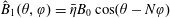 $\hat{B}_{1}(\unicode[STIX]{x1D703},\unicode[STIX]{x1D711})=\bar{\unicode[STIX]{x1D702}}B_{0}\cos (\unicode[STIX]{x1D703}-N\unicode[STIX]{x1D711})$
for constant
$\hat{B}_{1}(\unicode[STIX]{x1D703},\unicode[STIX]{x1D711})=\bar{\unicode[STIX]{x1D702}}B_{0}\cos (\unicode[STIX]{x1D703}-N\unicode[STIX]{x1D711})$
for constant
 $\bar{\unicode[STIX]{x1D702}}$
, where
$\bar{\unicode[STIX]{x1D702}}$
, where
 $N$
is allowed to be zero or non-zero, and let us take
$N$
is allowed to be zero or non-zero, and let us take
 $\bar{\unicode[STIX]{x1D702}}>0$
without loss of generality. Now consider a vector pointing perpendicularly from the axis to the
$\bar{\unicode[STIX]{x1D702}}>0$
without loss of generality. Now consider a vector pointing perpendicularly from the axis to the
 $\unicode[STIX]{x1D703}-N\unicode[STIX]{x1D711}=0$
curve on the first-order-in-
$\unicode[STIX]{x1D703}-N\unicode[STIX]{x1D711}=0$
curve on the first-order-in-
 $r$
flux surface, which equivalently points to the maximum-
$r$
flux surface, which equivalently points to the maximum-
 $B$
contour on the surface. From (3.1) and (3.7), this vector is
$B$
contour on the surface. From (3.1) and (3.7), this vector is
 $\boldsymbol{n}r\bar{\unicode[STIX]{x1D702}}/\unicode[STIX]{x1D705}+\boldsymbol{b}rY_{1}$
, which has a positive projection along
$\boldsymbol{n}r\bar{\unicode[STIX]{x1D702}}/\unicode[STIX]{x1D705}+\boldsymbol{b}rY_{1}$
, which has a positive projection along
 $\boldsymbol{n}$
at all
$\boldsymbol{n}$
at all
 $\unicode[STIX]{x1D711}$
. Therefore this vector to the maximum-
$\unicode[STIX]{x1D711}$
. Therefore this vector to the maximum-
 $B$
curve never points in a direction more than
$B$
curve never points in a direction more than
 $90^{\circ }$
away from the normal vector
$90^{\circ }$
away from the normal vector
 $\boldsymbol{n}$
. Hence, in a full toroidal transit around the axis, the
$\boldsymbol{n}$
. Hence, in a full toroidal transit around the axis, the
 $\unicode[STIX]{x1D703}-N\unicode[STIX]{x1D711}=0$
curve must wrap poloidally around the magnetic axis the same number of times
$\unicode[STIX]{x1D703}-N\unicode[STIX]{x1D711}=0$
curve must wrap poloidally around the magnetic axis the same number of times
 $\boldsymbol{n}$
does so. Therefore,
$\boldsymbol{n}$
does so. Therefore,
 $N$
is the number of times
$N$
is the number of times
 $\boldsymbol{n}$
rotates poloidally around the axis in a full toroidal transit of the axis. If
$\boldsymbol{n}$
rotates poloidally around the axis in a full toroidal transit of the axis. If
 $\boldsymbol{n}$
does not have such a net rotation for a given axis shape, then all quasi-symmetric solutions for this axis shape will be quasi-axisymmetric, whereas if
$\boldsymbol{n}$
does not have such a net rotation for a given axis shape, then all quasi-symmetric solutions for this axis shape will be quasi-axisymmetric, whereas if
 $\boldsymbol{n}$
does have this net rotation, all quasi-symmetric solutions for this axis shape will be quasi-helically symmetric.
$\boldsymbol{n}$
does have this net rotation, all quasi-symmetric solutions for this axis shape will be quasi-helically symmetric.
For another perspective on
 $N$
, consider that because of (5.3), in the derivation of (3.13), (5.1) and (5.2), it was never imposed that
$N$
, consider that because of (5.3), in the derivation of (3.13), (5.1) and (5.2), it was never imposed that
 $\unicode[STIX]{x1D703}$
must be a poloidal angle rather than a helical angle. The choice of
$\unicode[STIX]{x1D703}$
must be a poloidal angle rather than a helical angle. The choice of
 $N$
in the previous paragraph finally eliminates this redundancy. If one solves the quasi-axisymmetry equation (5.1) for an axis shape that ‘really’ should have quasi-helical symmetry rather than quasi-axisymmetry, one finds that the
$N$
in the previous paragraph finally eliminates this redundancy. If one solves the quasi-axisymmetry equation (5.1) for an axis shape that ‘really’ should have quasi-helical symmetry rather than quasi-axisymmetry, one finds that the
 $\unicode[STIX]{x1D703}=0$
curve on each flux surface wraps around the axis poloidally as you traverse the axis toroidally, i.e.
$\unicode[STIX]{x1D703}=0$
curve on each flux surface wraps around the axis poloidally as you traverse the axis toroidally, i.e.
 $\unicode[STIX]{x1D703}$
turns out to be a helical angle rather than a poloidal angle.
$\unicode[STIX]{x1D703}$
turns out to be a helical angle rather than a poloidal angle.
Numerical solution of (5.1)–(5.2) as a practical method to construct and parameterize quasi-symmetric equilibria will be demonstrated in Part 2.
5.3 Necessity of axis torsion
Note that
 $\unicode[STIX]{x1D70F}=0$
implies the magnetic axis and
$\unicode[STIX]{x1D70F}=0$
implies the magnetic axis and
 $\boldsymbol{n}$
are confined to a plane, so
$\boldsymbol{n}$
are confined to a plane, so
 $\boldsymbol{n}$
cannot rotate poloidally about the magnetic axis. Then by the argument in the preceding section,
$\boldsymbol{n}$
cannot rotate poloidally about the magnetic axis. Then by the argument in the preceding section,
 $\unicode[STIX]{x1D70F}=0$
can only be consistent with quasi-axisymmetry, not quasi-helical symmetry. Moreover, in a stellarator,
$\unicode[STIX]{x1D70F}=0$
can only be consistent with quasi-axisymmetry, not quasi-helical symmetry. Moreover, in a stellarator,
 $I_{2}$
(which represents the on-axis density of toroidal current) is typically zero, as the bootstrap current vanishes on axis. In this case, if
$I_{2}$
(which represents the on-axis density of toroidal current) is typically zero, as the bootstrap current vanishes on axis. In this case, if
 $\unicode[STIX]{x1D70F}=0$
, the integral of (5.1) gives
$\unicode[STIX]{x1D70F}=0$
, the integral of (5.1) gives
 $$\begin{eqnarray}\unicode[STIX]{x1D704}_{0}\int _{0}^{2\unicode[STIX]{x03C0}}\text{d}\unicode[STIX]{x1D711}\left[\frac{\hat{B}_{1c}^{4}}{B_{0}^{4}\unicode[STIX]{x1D705}^{4}}+1+\unicode[STIX]{x1D70E}^{2}\right]=0.\end{eqnarray}$$
The integral is positive–definite, so
 $\unicode[STIX]{x1D704}_{0}$
must vanish. Therefore, torsion of the magnetic axis is essential in a quasi-symmetric stellarator in order to have rotational transform on axis.
$\unicode[STIX]{x1D704}_{0}$
must vanish. Therefore, torsion of the magnetic axis is essential in a quasi-symmetric stellarator in order to have rotational transform on axis.
6 Discussion and conclusions
In this paper, we have derived the relationship near the magnetic axis between the flux surface shape in cylindrical coordinates and the magnetic field strength
 $B(r,\unicode[STIX]{x1D703},\unicode[STIX]{x1D711})$
in Boozer coordinates. This relationship is important for stellarator design since
$B(r,\unicode[STIX]{x1D703},\unicode[STIX]{x1D711})$
in Boozer coordinates. This relationship is important for stellarator design since
 $B(r,\unicode[STIX]{x1D703},\unicode[STIX]{x1D711})$
essentially determines the guiding-centre confinement, but it is the flux surface shape in three dimensions that determines the coils and engineering design. As part of this calculation, we have also derived the relationship between the flux surface shape in cylindrical coordinates and the rotational transform. No matter how low the aspect ratio of a stellarator, the analysis here applies in a region sufficiently close to the axis. The result of this analysis is the system of equations (2.24), (2.30)–(2.32) or (4.9), and (2.34)–(2.36). These equations can be derived directly in cylindrical coordinates, as in § 2, or by the appropriate transformation of Garren & Boozer’s equations, using the transformation of § 4.1. In contrast to the calculation of Garren & Boozer (Reference Garren and Boozer1991a
), the equations here remain regular on segments or points where the axis torsion vanishes, which always occurs for omnigenous fields with poloidally closed
$B(r,\unicode[STIX]{x1D703},\unicode[STIX]{x1D711})$
essentially determines the guiding-centre confinement, but it is the flux surface shape in three dimensions that determines the coils and engineering design. As part of this calculation, we have also derived the relationship between the flux surface shape in cylindrical coordinates and the rotational transform. No matter how low the aspect ratio of a stellarator, the analysis here applies in a region sufficiently close to the axis. The result of this analysis is the system of equations (2.24), (2.30)–(2.32) or (4.9), and (2.34)–(2.36). These equations can be derived directly in cylindrical coordinates, as in § 2, or by the appropriate transformation of Garren & Boozer’s equations, using the transformation of § 4.1. In contrast to the calculation of Garren & Boozer (Reference Garren and Boozer1991a
), the equations here remain regular on segments or points where the axis torsion vanishes, which always occurs for omnigenous fields with poloidally closed
 $B$
contours. The torsion, which may not be well defined in this circumstance, does not appear in our analysis since we avoid using the Frenet–Serret frame.
$B$
contours. The torsion, which may not be well defined in this circumstance, does not appear in our analysis since we avoid using the Frenet–Serret frame.
Consistent with Garren & Boozer (Reference Garren and Boozer1991a
), we find that at
 $O(r^{1})$
, for a prescribed
$O(r^{1})$
, for a prescribed
 $B_{1}$
, there are two more
$B_{1}$
, there are two more
 $\unicode[STIX]{x1D719}$
-dependent degrees of freedom than there are equations. Specifically, the six
$\unicode[STIX]{x1D719}$
-dependent degrees of freedom than there are equations. Specifically, the six
 $\unicode[STIX]{x1D719}$
-dependent unknowns (
$\unicode[STIX]{x1D719}$
-dependent unknowns (
 $R_{0}$
,
$R_{0}$
,
 $z_{0}$
,
$z_{0}$
,
 $R_{1c}$
,
$R_{1c}$
,
 $R_{1s}$
,
$R_{1s}$
,
 $z_{1c}$
and
$z_{1c}$
and
 $z_{1s}$
) are constrained by four equations: (2.24), the
$z_{1s}$
) are constrained by four equations: (2.24), the
 $\sin \unicode[STIX]{x1D703}$
and
$\sin \unicode[STIX]{x1D703}$
and
 $\cos \unicode[STIX]{x1D703}$
components of (2.30), and (2.34). Thus, two of these six functions can be viewed as inputs. Choosing
$\cos \unicode[STIX]{x1D703}$
components of (2.30), and (2.34). Thus, two of these six functions can be viewed as inputs. Choosing
 $R_{0}$
and
$R_{0}$
and
 $z_{0}$
as the two inputs amounts to specifying the magnetic axis shape, and the four aforementioned equations then give the flux surface shape that yields the desired
$z_{0}$
as the two inputs amounts to specifying the magnetic axis shape, and the four aforementioned equations then give the flux surface shape that yields the desired
 $B_{1}$
.
$B_{1}$
.
Acknowledgements
We acknowledge illuminating conversations about this work with G. Plunk. This work was supported by the U.S. Department of Energy, Office of Science, Office of Fusion Energy Science, under award numbers DE-FG02-93ER54197 and DE-FG02-86ER53223. This work was also supported by a grant from the Simons Foundation (560651, M.L.)
Appendix A. Regularity near the magnetic axis
In this section we will derive the form of the expansion (2.12)–(2.14) for
 $R$
,
$R$
,
 $z$
,
$z$
,
 $\unicode[STIX]{x1D708}$
and
$\unicode[STIX]{x1D708}$
and
 $B$
. As an alternative to the argument based on analyticity in Garren & Boozer (Reference Garren and Boozer1991a
), here we give a constructive demonstration, proceeding in several steps. First, we will derive the form (2.12)–(2.14) for
$B$
. As an alternative to the argument based on analyticity in Garren & Boozer (Reference Garren and Boozer1991a
), here we give a constructive demonstration, proceeding in several steps. First, we will derive the form (2.12)–(2.14) for
 $R$
and
$R$
and
 $z$
but with a non-straight-field-line poloidal angle
$z$
but with a non-straight-field-line poloidal angle
 $\unicode[STIX]{x1D6FC}$
in place of the Boozer angle
$\unicode[STIX]{x1D6FC}$
in place of the Boozer angle
 $\unicode[STIX]{x1D703}$
. Then we will derive the form (2.12)–(2.14) for
$\unicode[STIX]{x1D703}$
. Then we will derive the form (2.12)–(2.14) for
 $R$
and
$R$
and
 $z$
but with the poloidal angle
$z$
but with the poloidal angle
 $\unicode[STIX]{x1D709}$
defined such that field lines are straight in the
$\unicode[STIX]{x1D709}$
defined such that field lines are straight in the
 $\unicode[STIX]{x1D709}$
–
$\unicode[STIX]{x1D709}$
–
 $\unicode[STIX]{x1D719}$
plane. Next, we will derive (2.12)–(2.14) for
$\unicode[STIX]{x1D719}$
plane. Next, we will derive (2.12)–(2.14) for
 $\unicode[STIX]{x1D703}$
. Finally, we extend the proof to
$\unicode[STIX]{x1D703}$
. Finally, we extend the proof to
 $\unicode[STIX]{x1D708}$
and
$\unicode[STIX]{x1D708}$
and
 $B$
.
$B$
.
Assuming good flux surfaces exist near the axis, a Taylor expansion exists for
 $\unicode[STIX]{x1D713}(R,z)$
:
$\unicode[STIX]{x1D713}(R,z)$
:
 $$\begin{eqnarray}\displaystyle \unicode[STIX]{x1D713} & = & \displaystyle \frac{(R-R_{0})^{2}}{2}\unicode[STIX]{x1D713}_{RR}+(R-R_{0})(z-z_{0})\unicode[STIX]{x1D713}_{Rz}+\frac{(z-z_{0})^{2}}{2}\unicode[STIX]{x1D713}_{zz}+\frac{(R-R_{0})^{3}}{6}\unicode[STIX]{x1D713}_{RRR}\nonumber\\ \displaystyle & & \displaystyle +\,\frac{(R-R_{0})^{2}(z-z_{0})}{2}\unicode[STIX]{x1D713}_{RRz}+\frac{(R-R_{0})(z-z_{0})^{2}}{2}\unicode[STIX]{x1D713}_{Rzz}+\frac{(z-z_{0})^{3}}{6}\unicode[STIX]{x1D713}_{zzz}+\cdots \,,\qquad\end{eqnarray}$$
where quantities such as
 $\unicode[STIX]{x1D713}_{RR}$
refer to partial derivatives evaluated at the axis
$\unicode[STIX]{x1D713}_{RR}$
refer to partial derivatives evaluated at the axis
 $(R_{0},z_{0})$
, and dependence on the independent variable
$(R_{0},z_{0})$
, and dependence on the independent variable
 $\unicode[STIX]{x1D719}$
is not displayed to simplify notation. Note
$\unicode[STIX]{x1D719}$
is not displayed to simplify notation. Note
 $A>0$
where
$A>0$
where
 $A=\unicode[STIX]{x1D713}_{RR}\unicode[STIX]{x1D713}_{zz}-\unicode[STIX]{x1D713}_{Rz}^{2}$
, since the axis is an extremum of
$A=\unicode[STIX]{x1D713}_{RR}\unicode[STIX]{x1D713}_{zz}-\unicode[STIX]{x1D713}_{Rz}^{2}$
, since the axis is an extremum of
 $\unicode[STIX]{x1D713}$
rather than a saddle point. For this section we assume
$\unicode[STIX]{x1D713}$
rather than a saddle point. For this section we assume
 $\unicode[STIX]{x1D713}_{RR}$
and
$\unicode[STIX]{x1D713}_{RR}$
and
 $\unicode[STIX]{x1D713}_{zz}$
are positive for simplicity, so
$\unicode[STIX]{x1D713}_{zz}$
are positive for simplicity, so
 $\unicode[STIX]{x1D713}\geqslant 0$
. We then seek a solution of the desired form:
$\unicode[STIX]{x1D713}\geqslant 0$
. We then seek a solution of the desired form:
 $$\begin{eqnarray}\left.\begin{array}{@{}c@{}}R=R_{0}+r(R_{1c}^{\unicode[STIX]{x1D6FC}}\cos \unicode[STIX]{x1D6FC}+R_{1s}^{\unicode[STIX]{x1D6FC}}\sin \unicode[STIX]{x1D6FC})+r^{2}(R_{20}^{\unicode[STIX]{x1D6FC}}+R_{2c}^{\unicode[STIX]{x1D6FC}}\cos 2\unicode[STIX]{x1D6FC}+R_{2s}^{\unicode[STIX]{x1D6FC}}\sin 2\unicode[STIX]{x1D6FC})+O(r^{3}),\\ z=z_{0}+r(z_{1c}^{\unicode[STIX]{x1D6FC}}\cos \unicode[STIX]{x1D6FC}+z_{1s}^{\unicode[STIX]{x1D6FC}}\sin \unicode[STIX]{x1D6FC})+r^{2}(z_{20}^{\unicode[STIX]{x1D6FC}}+z_{2c}^{\unicode[STIX]{x1D6FC}}\cos 2\unicode[STIX]{x1D6FC}+z_{2s}^{\unicode[STIX]{x1D6FC}}\sin 2\unicode[STIX]{x1D6FC})+O(r^{3}).\end{array}\right\}\end{eqnarray}$$
Substituting (A 2) into (A 1), terms can be collected based on their order in
 $r$
and
$r$
and
 $\unicode[STIX]{x1D6FC}$
dependence. The number of equations that result at a given order in
$\unicode[STIX]{x1D6FC}$
dependence. The number of equations that result at a given order in
 $r$
is smaller than the number of associated coefficients in (A 2), reflecting the non-uniqueness of the poloidal angle; for instance the
$r$
is smaller than the number of associated coefficients in (A 2), reflecting the non-uniqueness of the poloidal angle; for instance the
 $\unicode[STIX]{x1D6FC}=0$
direction can be shifted. One solution satisfying (A 1) through
$\unicode[STIX]{x1D6FC}=0$
direction can be shifted. One solution satisfying (A 1) through
 $O(r^{3})$
is
$O(r^{3})$
is
 $z_{1c}^{\unicode[STIX]{x1D6FC}}=0$
,
$z_{1c}^{\unicode[STIX]{x1D6FC}}=0$
,
 $R_{20}^{\unicode[STIX]{x1D6FC}}=0$
,
$R_{20}^{\unicode[STIX]{x1D6FC}}=0$
,
 $$\begin{eqnarray}\left.\begin{array}{@{}l@{}}\displaystyle R_{1c}^{\unicode[STIX]{x1D6FC}}=\sqrt{\frac{\bar{B}}{\unicode[STIX]{x1D713}_{RR}}},\quad R_{1s}^{\unicode[STIX]{x1D6FC}}=\unicode[STIX]{x1D713}_{Rz}\sqrt{\frac{\bar{B}}{\unicode[STIX]{x1D713}_{RR}A}},\quad z_{1s}^{\unicode[STIX]{x1D6FC}}=-\sqrt{\frac{\bar{B}\unicode[STIX]{x1D713}_{RR}}{A}},\quad R_{2c}^{\unicode[STIX]{x1D6FC}}=-\frac{\bar{B}\unicode[STIX]{x1D713}_{RRR}}{6\unicode[STIX]{x1D713}_{RR}^{2}},\\ \displaystyle R_{2s}^{\unicode[STIX]{x1D6FC}}=-\frac{\bar{B}}{12\unicode[STIX]{x1D713}_{RR}^{2}A^{5/2}}\left[\unicode[STIX]{x1D713}_{RRR}(4\unicode[STIX]{x1D713}_{RR}^{2}\unicode[STIX]{x1D713}_{Rz}\unicode[STIX]{x1D713}_{zz}^{2}-5\unicode[STIX]{x1D713}_{RR}\unicode[STIX]{x1D713}_{Rz}^{3}\unicode[STIX]{x1D713}_{zz}+2\unicode[STIX]{x1D713}_{Rz}^{5})\right.\\ \displaystyle \qquad \left.-\unicode[STIX]{x1D713}_{RR}^{3}(3\unicode[STIX]{x1D713}_{RRz}\unicode[STIX]{x1D713}_{zz}^{2}+\unicode[STIX]{x1D713}_{Rz}^{2}\unicode[STIX]{x1D713}_{zzz}-3\unicode[STIX]{x1D713}_{Rz}\unicode[STIX]{x1D713}_{Rzz}\unicode[STIX]{x1D713}_{zz})\right],\\ \displaystyle z_{2c}^{\unicode[STIX]{x1D6FC}}=-z_{20}^{\unicode[STIX]{x1D6FC}}=\frac{\bar{B}}{12\unicode[STIX]{x1D713}_{RR}A^{2}}\left[\unicode[STIX]{x1D713}_{RR}^{3}\unicode[STIX]{x1D713}_{zzz}-3\unicode[STIX]{x1D713}_{RR}^{2}\unicode[STIX]{x1D713}_{Rz}\unicode[STIX]{x1D713}_{Rzz}+3\unicode[STIX]{x1D713}_{RR}\unicode[STIX]{x1D713}_{RRz}\unicode[STIX]{x1D713}_{Rz}^{2}-\unicode[STIX]{x1D713}_{RRR}\unicode[STIX]{x1D713}_{Rz}^{3}\right],\\ \displaystyle z_{2s}^{\unicode[STIX]{x1D6FC}}=-\frac{\bar{B}}{12\unicode[STIX]{x1D713}_{RR}A^{5/2}}\left[\unicode[STIX]{x1D713}_{RR}^{3}(\unicode[STIX]{x1D713}_{Rz}\unicode[STIX]{x1D713}_{zzz}-3\unicode[STIX]{x1D713}_{Rzz}\unicode[STIX]{x1D713}_{zz})+\unicode[STIX]{x1D713}_{RR}^{2}\unicode[STIX]{x1D713}_{zz}(6\unicode[STIX]{x1D713}_{RRz}\unicode[STIX]{x1D713}_{Rz}-\unicode[STIX]{x1D713}_{RRR}\unicode[STIX]{x1D713}_{zz})\right.\\ \displaystyle \qquad \left.-\unicode[STIX]{x1D713}_{RR}\unicode[STIX]{x1D713}_{Rz}^{2}(\unicode[STIX]{x1D713}_{RRR}\unicode[STIX]{x1D713}_{zz}+3\unicode[STIX]{x1D713}_{RRz}\unicode[STIX]{x1D713}_{Rz})+\unicode[STIX]{x1D713}_{RRR}\unicode[STIX]{x1D713}_{Rz}^{4}\right].\end{array}\right\}\end{eqnarray}$$
Thus, given the Taylor series for
 $\unicode[STIX]{x1D713}(R,z)$
, we can construct expansions of the form (2.12)–(2.14), but with
$\unicode[STIX]{x1D713}(R,z)$
, we can construct expansions of the form (2.12)–(2.14), but with
 $\unicode[STIX]{x1D703}\rightarrow \unicode[STIX]{x1D6FC}$
, for
$\unicode[STIX]{x1D703}\rightarrow \unicode[STIX]{x1D6FC}$
, for
 $R$
and
$R$
and
 $z$
. The
$z$
. The
 $O(r)$
terms in (A 2) can be manipulated to write the poloidal angle explicitly as
$O(r)$
terms in (A 2) can be manipulated to write the poloidal angle explicitly as
 $$\begin{eqnarray}\unicode[STIX]{x1D6FC}\approx \text{atan2}(-(z-z_{0}),[(R-R_{0})\unicode[STIX]{x1D713}_{RR}+(z-z_{0})\unicode[STIX]{x1D713}_{Rz}]/\sqrt{A}),\end{eqnarray}$$
where atan2 is the arctangent with range
 $(-\unicode[STIX]{x03C0},\unicode[STIX]{x03C0}]$
.
$(-\unicode[STIX]{x03C0},\unicode[STIX]{x03C0}]$
.
Next we construct the straight-field-line angle
 $\unicode[STIX]{x1D709}=\unicode[STIX]{x1D6FC}+\unicode[STIX]{x1D706}$
where
$\unicode[STIX]{x1D709}=\unicode[STIX]{x1D6FC}+\unicode[STIX]{x1D706}$
where
 $\unicode[STIX]{x1D706}(r,\unicode[STIX]{x1D6FC},\unicode[STIX]{x1D719})$
is single valued. From the
$\unicode[STIX]{x1D706}(r,\unicode[STIX]{x1D6FC},\unicode[STIX]{x1D719})$
is single valued. From the
 $\unicode[STIX]{x1D735}\unicode[STIX]{x1D719}$
component of
$\unicode[STIX]{x1D735}\unicode[STIX]{x1D719}$
component of
 $\boldsymbol{B}=\unicode[STIX]{x1D735}\unicode[STIX]{x1D713}\times \unicode[STIX]{x1D735}\unicode[STIX]{x1D709}+\unicode[STIX]{x1D704}\unicode[STIX]{x1D735}\unicode[STIX]{x1D719}\times \unicode[STIX]{x1D735}\unicode[STIX]{x1D713}$
, we find
$\boldsymbol{B}=\unicode[STIX]{x1D735}\unicode[STIX]{x1D713}\times \unicode[STIX]{x1D735}\unicode[STIX]{x1D709}+\unicode[STIX]{x1D704}\unicode[STIX]{x1D735}\unicode[STIX]{x1D719}\times \unicode[STIX]{x1D735}\unicode[STIX]{x1D713}$
, we find
 $$\begin{eqnarray}\unicode[STIX]{x1D706}=f(r,\unicode[STIX]{x1D719})+\int _{0}^{\unicode[STIX]{x1D6FC}}\text{d}\unicode[STIX]{x1D6FC}^{\prime }\left[\left(\frac{\unicode[STIX]{x2202}\boldsymbol{r}}{\unicode[STIX]{x2202}\unicode[STIX]{x1D713}}\boldsymbol{\cdot }\frac{\unicode[STIX]{x2202}\boldsymbol{r}}{\unicode[STIX]{x2202}\unicode[STIX]{x1D6FC}}\times \frac{\unicode[STIX]{x2202}\boldsymbol{r}}{\unicode[STIX]{x2202}\unicode[STIX]{x1D719}}\right)\boldsymbol{B}\boldsymbol{\cdot }\unicode[STIX]{x1D735}\unicode[STIX]{x1D719}-1\right],\end{eqnarray}$$
for some
 $f(r,\unicode[STIX]{x1D719})$
. The Jacobian in this expression can be evaluated using derivatives of
$f(r,\unicode[STIX]{x1D719})$
. The Jacobian in this expression can be evaluated using derivatives of
 $\boldsymbol{r}=R\boldsymbol{e}_{R}+z\boldsymbol{e}_{z}$
; substitution of (A 2) then yields
$\boldsymbol{r}=R\boldsymbol{e}_{R}+z\boldsymbol{e}_{z}$
; substitution of (A 2) then yields
 $$\begin{eqnarray}\frac{\unicode[STIX]{x2202}\boldsymbol{r}}{\unicode[STIX]{x2202}\unicode[STIX]{x1D713}}\boldsymbol{\cdot }\frac{\unicode[STIX]{x2202}\boldsymbol{r}}{\unicode[STIX]{x2202}\unicode[STIX]{x1D6FC}}\times \frac{\unicode[STIX]{x2202}\boldsymbol{r}}{\unicode[STIX]{x2202}\unicode[STIX]{x1D719}}=\left(\frac{\unicode[STIX]{x2202}z}{\unicode[STIX]{x2202}\unicode[STIX]{x1D713}}\frac{\unicode[STIX]{x2202}R}{\unicode[STIX]{x2202}\unicode[STIX]{x1D6FC}}-\frac{\unicode[STIX]{x2202}z}{\unicode[STIX]{x2202}\unicode[STIX]{x1D6FC}}\frac{\unicode[STIX]{x2202}R}{\unicode[STIX]{x2202}\unicode[STIX]{x1D713}}\right)R=\frac{R_{0}}{\sqrt{A}}\left(1+rJ_{1s}\sin \unicode[STIX]{x1D6FC}+rJ_{1c}\cos \unicode[STIX]{x1D6FC}+O(r^{2})\right),\end{eqnarray}$$
where
 $J_{1s}$
and
$J_{1s}$
and
 $J_{1c}$
are complicated algebraic functions of the Taylor coefficients in (A 1). Also, in (A 5),
$J_{1c}$
are complicated algebraic functions of the Taylor coefficients in (A 1). Also, in (A 5),
 $\boldsymbol{B}\boldsymbol{\cdot }\unicode[STIX]{x1D735}\unicode[STIX]{x1D719}$
is smooth so it has a Taylor series
$\boldsymbol{B}\boldsymbol{\cdot }\unicode[STIX]{x1D735}\unicode[STIX]{x1D719}$
is smooth so it has a Taylor series
 $$\begin{eqnarray}\boldsymbol{B}\boldsymbol{\cdot }\unicode[STIX]{x1D735}\unicode[STIX]{x1D719}=b_{0}+(R-R_{0})b_{R}+(z-z_{0})b_{z}+O(r^{2}).\end{eqnarray}$$
Using the
 $O(r)$
terms in (A 2) and (A 3) in (B 3) for the area of an ellipse, flux surfaces near the axis have an area
$O(r)$
terms in (A 2) and (A 3) in (B 3) for the area of an ellipse, flux surfaces near the axis have an area
 $2\unicode[STIX]{x03C0}\unicode[STIX]{x1D713}/\sqrt{A}$
in the
$2\unicode[STIX]{x03C0}\unicode[STIX]{x1D713}/\sqrt{A}$
in the
 $R$
–
$R$
–
 $z$
plane, so
$z$
plane, so
 $b_{0}=\sqrt{A}/R_{0}$
. Evaluating the integral in (A 5) then gives
$b_{0}=\sqrt{A}/R_{0}$
. Evaluating the integral in (A 5) then gives
 $$\begin{eqnarray}\unicode[STIX]{x1D706}=\hat{f}(r,\unicode[STIX]{x1D719})+r\unicode[STIX]{x1D706}_{1s}\sin \unicode[STIX]{x1D6FC}+r\unicode[STIX]{x1D706}_{1c}\cos \unicode[STIX]{x1D6FC}+O(r^{2}),\end{eqnarray}$$
where
 $\unicode[STIX]{x1D706}_{1s}=b_{R}R_{1c}^{\unicode[STIX]{x1D6FC}}R_{0}/\sqrt{A}+J_{1c}$
,
$\unicode[STIX]{x1D706}_{1s}=b_{R}R_{1c}^{\unicode[STIX]{x1D6FC}}R_{0}/\sqrt{A}+J_{1c}$
,
 $\unicode[STIX]{x1D706}_{1c}=-J_{1s}-(b_{R}R_{1s}^{\unicode[STIX]{x1D6FC}}+b_{z}z_{1s}^{\unicode[STIX]{x1D6FC}})R_{0}/\sqrt{A}$
and
$\unicode[STIX]{x1D706}_{1c}=-J_{1s}-(b_{R}R_{1s}^{\unicode[STIX]{x1D6FC}}+b_{z}z_{1s}^{\unicode[STIX]{x1D6FC}})R_{0}/\sqrt{A}$
and
 $\hat{f}=f-r\unicode[STIX]{x1D706}_{1c}$
. To constrain the form of
$\hat{f}=f-r\unicode[STIX]{x1D706}_{1c}$
. To constrain the form of
 $\hat{f}$
, we use the
$\hat{f}$
, we use the
 $\unicode[STIX]{x1D735}\unicode[STIX]{x1D6FC}$
component of
$\unicode[STIX]{x1D735}\unicode[STIX]{x1D6FC}$
component of
 $\boldsymbol{B}=\unicode[STIX]{x1D735}\unicode[STIX]{x1D713}\times \unicode[STIX]{x1D735}\unicode[STIX]{x1D709}+\unicode[STIX]{x1D704}\unicode[STIX]{x1D735}\unicode[STIX]{x1D719}\times \unicode[STIX]{x1D735}\unicode[STIX]{x1D713}$
to write
$\boldsymbol{B}=\unicode[STIX]{x1D735}\unicode[STIX]{x1D713}\times \unicode[STIX]{x1D735}\unicode[STIX]{x1D709}+\unicode[STIX]{x1D704}\unicode[STIX]{x1D735}\unicode[STIX]{x1D719}\times \unicode[STIX]{x1D735}\unicode[STIX]{x1D713}$
to write
 $$\begin{eqnarray}\frac{\unicode[STIX]{x2202}\unicode[STIX]{x1D706}}{\unicode[STIX]{x2202}\unicode[STIX]{x1D719}}=\unicode[STIX]{x1D704}-\frac{\boldsymbol{B}\boldsymbol{\cdot }\unicode[STIX]{x1D735}\unicode[STIX]{x1D6FC}}{\unicode[STIX]{x1D735}\unicode[STIX]{x1D713}\boldsymbol{\cdot }\unicode[STIX]{x1D735}\unicode[STIX]{x1D6FC}\times \unicode[STIX]{x1D735}\unicode[STIX]{x1D719}}=\unicode[STIX]{x1D704}-\boldsymbol{B}\boldsymbol{\cdot }\frac{\unicode[STIX]{x2202}\boldsymbol{r}}{\unicode[STIX]{x2202}\unicode[STIX]{x1D719}}\times \frac{\unicode[STIX]{x2202}\boldsymbol{r}}{\unicode[STIX]{x2202}\unicode[STIX]{x1D713}}.\end{eqnarray}$$
In the last term, note that
 $\boldsymbol{B}$
has a Taylor expansion in
$\boldsymbol{B}$
has a Taylor expansion in
 $R-R_{0}$
and
$R-R_{0}$
and
 $z-z_{0}$
like (A 7) but with vector coefficients; the leading term is parallel to
$z-z_{0}$
like (A 7) but with vector coefficients; the leading term is parallel to
 $\unicode[STIX]{x2202}\boldsymbol{r}/\unicode[STIX]{x2202}\unicode[STIX]{x1D719}$
, so the last term in (A 9) is finite on the axis. Evaluating the last term in (A 9) by differentiating
$\unicode[STIX]{x2202}\boldsymbol{r}/\unicode[STIX]{x2202}\unicode[STIX]{x1D719}$
, so the last term in (A 9) is finite on the axis. Evaluating the last term in (A 9) by differentiating
 $\boldsymbol{r}=R\boldsymbol{e}_{R}+z\boldsymbol{e}_{z}$
and substituting (A 2), and applying
$\boldsymbol{r}=R\boldsymbol{e}_{R}+z\boldsymbol{e}_{z}$
and substituting (A 2), and applying
 $\int _{0}^{2\unicode[STIX]{x03C0}}\text{d}\unicode[STIX]{x1D6FC}\;\unicode[STIX]{x2202}(\ldots )/\unicode[STIX]{x2202}r$
to (A 9), we find
$\int _{0}^{2\unicode[STIX]{x03C0}}\text{d}\unicode[STIX]{x1D6FC}\;\unicode[STIX]{x2202}(\ldots )/\unicode[STIX]{x2202}r$
to (A 9), we find
 $\int _{0}^{2\unicode[STIX]{x03C0}}\text{d}\unicode[STIX]{x1D6FC}\;\unicode[STIX]{x2202}^{2}\unicode[STIX]{x1D706}/\unicode[STIX]{x2202}r\unicode[STIX]{x2202}\unicode[STIX]{x1D719}=0$
at
$\int _{0}^{2\unicode[STIX]{x03C0}}\text{d}\unicode[STIX]{x1D6FC}\;\unicode[STIX]{x2202}^{2}\unicode[STIX]{x1D706}/\unicode[STIX]{x2202}r\unicode[STIX]{x2202}\unicode[STIX]{x1D719}=0$
at
 $r=0$
, which implies the
$r=0$
, which implies the
 $O(r)$
term of
$O(r)$
term of
 $\hat{f}$
is independent of
$\hat{f}$
is independent of
 $\unicode[STIX]{x1D719}$
. This term can therefore be set to 0, since
$\unicode[STIX]{x1D719}$
. This term can therefore be set to 0, since
 $\unicode[STIX]{x1D706}$
can be shifted by any function of only
$\unicode[STIX]{x1D706}$
can be shifted by any function of only
 $r$
. Hence,
$r$
. Hence,
 $$\begin{eqnarray}\unicode[STIX]{x1D706}=\unicode[STIX]{x1D706}_{0}+r\unicode[STIX]{x1D706}_{1s}\sin \unicode[STIX]{x1D6FC}+r\unicode[STIX]{x1D706}_{1c}\cos \unicode[STIX]{x1D6FC}+O(r^{2}),\end{eqnarray}$$
for some
 $\unicode[STIX]{x1D706}_{0}(\unicode[STIX]{x1D719})$
. Substituting
$\unicode[STIX]{x1D706}_{0}(\unicode[STIX]{x1D719})$
. Substituting
 $\unicode[STIX]{x1D6FC}=\unicode[STIX]{x1D709}-\unicode[STIX]{x1D706}$
and (A 10) into (A 2), we obtain an expansion of the desired form:
$\unicode[STIX]{x1D6FC}=\unicode[STIX]{x1D709}-\unicode[STIX]{x1D706}$
and (A 10) into (A 2), we obtain an expansion of the desired form:
 $$\begin{eqnarray}\left.\begin{array}{@{}c@{}}\displaystyle R=R_{0}+r(R_{1c}^{\unicode[STIX]{x1D709}}\cos \unicode[STIX]{x1D709}+R_{1s}^{\unicode[STIX]{x1D709}}\sin \unicode[STIX]{x1D709})+r^{2}(R_{20}^{\unicode[STIX]{x1D709}}+R_{2c}^{\unicode[STIX]{x1D709}}\cos 2\unicode[STIX]{x1D709}+R_{2s}^{\unicode[STIX]{x1D709}}\sin 2\unicode[STIX]{x1D709})+O(r^{3}),\\ \displaystyle z=z_{0}+r(z_{1c}^{\unicode[STIX]{x1D709}}\cos \unicode[STIX]{x1D709}+z_{1s}^{\unicode[STIX]{x1D709}}\sin \unicode[STIX]{x1D709})+r^{2}(z_{20}^{\unicode[STIX]{x1D709}}+z_{2c}^{\unicode[STIX]{x1D709}}\cos 2\unicode[STIX]{x1D709}+z_{2s}^{\unicode[STIX]{x1D709}}\sin 2\unicode[STIX]{x1D709})+O(r^{3}),\end{array}\right\}\end{eqnarray}$$
where the
 $R^{\unicode[STIX]{x1D709}}$
and
$R^{\unicode[STIX]{x1D709}}$
and
 $z^{\unicode[STIX]{x1D709}}$
coefficients are functions of the
$z^{\unicode[STIX]{x1D709}}$
coefficients are functions of the
 $R^{\unicode[STIX]{x1D6FC}}$
and
$R^{\unicode[STIX]{x1D6FC}}$
and
 $z^{\unicode[STIX]{x1D6FC}}$
coefficients, e.g.
$z^{\unicode[STIX]{x1D6FC}}$
coefficients, e.g.
 $R_{1s}^{\unicode[STIX]{x1D709}}=R_{1s}^{\unicode[STIX]{x1D6FC}}\cos \unicode[STIX]{x1D706}_{0}+R_{1c}^{\unicode[STIX]{x1D6FC}}\sin \unicode[STIX]{x1D706}_{0}$
.
$R_{1s}^{\unicode[STIX]{x1D709}}=R_{1s}^{\unicode[STIX]{x1D6FC}}\cos \unicode[STIX]{x1D706}_{0}+R_{1c}^{\unicode[STIX]{x1D6FC}}\sin \unicode[STIX]{x1D706}_{0}$
.
Next we transform to Boozer coordinates. The magnetic field can be written (Helander Reference Helander2014) as
 $$\begin{eqnarray}\boldsymbol{B}=\hat{\unicode[STIX]{x1D6FD}}\unicode[STIX]{x1D735}\unicode[STIX]{x1D713}+I\unicode[STIX]{x1D735}\unicode[STIX]{x1D709}+G\unicode[STIX]{x1D735}\unicode[STIX]{x1D719}+\unicode[STIX]{x1D735}[(G+\unicode[STIX]{x1D704}I)\unicode[STIX]{x1D708}],\end{eqnarray}$$
for some
 $\hat{\unicode[STIX]{x1D6FD}}$
, where the transformation to Boozer coordinates is given by
$\hat{\unicode[STIX]{x1D6FD}}$
, where the transformation to Boozer coordinates is given by
 $\unicode[STIX]{x1D711}=\unicode[STIX]{x1D719}+\unicode[STIX]{x1D708}$
and
$\unicode[STIX]{x1D711}=\unicode[STIX]{x1D719}+\unicode[STIX]{x1D708}$
and
 $\unicode[STIX]{x1D703}=\unicode[STIX]{x1D709}+\unicode[STIX]{x1D704}\unicode[STIX]{x1D708}$
. Applying
$\unicode[STIX]{x1D703}=\unicode[STIX]{x1D709}+\unicode[STIX]{x1D704}\unicode[STIX]{x1D708}$
. Applying
 $\unicode[STIX]{x1D735}\unicode[STIX]{x1D719}\times \unicode[STIX]{x1D735}\unicode[STIX]{x1D713}\boldsymbol{\cdot }(\ldots )$
to (A 12), we find
$\unicode[STIX]{x1D735}\unicode[STIX]{x1D719}\times \unicode[STIX]{x1D735}\unicode[STIX]{x1D713}\boldsymbol{\cdot }(\ldots )$
to (A 12), we find
 $$\begin{eqnarray}\unicode[STIX]{x1D708}=g(r,\unicode[STIX]{x1D719})+\frac{1}{G+\unicode[STIX]{x1D704}I}\int _{0}^{\unicode[STIX]{x1D709}}\text{d}\unicode[STIX]{x1D709}^{\prime }\,\left[\frac{\boldsymbol{B}\boldsymbol{\cdot }\unicode[STIX]{x1D735}\unicode[STIX]{x1D719}\times \unicode[STIX]{x1D735}\unicode[STIX]{x1D713}}{\boldsymbol{B}\boldsymbol{\cdot }\unicode[STIX]{x1D735}\unicode[STIX]{x1D719}}-I\right].\end{eqnarray}$$
The denominator is smooth (and non-vanishing near the axis for cases of interest in this paper), with the expansion (A 7). The numerator is a product of three quantities that are smooth near the axis and so it too is smooth, vanishing on the axis since
 $\unicode[STIX]{x1D735}\unicode[STIX]{x1D713}=0$
there. Noting
$\unicode[STIX]{x1D735}\unicode[STIX]{x1D713}=0$
there. Noting
 $I$
is smooth function of
$I$
is smooth function of
 $\unicode[STIX]{x1D713}$
and
$\unicode[STIX]{x1D713}$
and
 $I=0$
on axis, then the quantity in square brackets in (A 13) is smooth and so has a Taylor expansion
$I=0$
on axis, then the quantity in square brackets in (A 13) is smooth and so has a Taylor expansion
 $$\begin{eqnarray}\displaystyle \frac{\boldsymbol{B}\boldsymbol{\cdot }\unicode[STIX]{x1D735}\unicode[STIX]{x1D719}\times \unicode[STIX]{x1D735}\unicode[STIX]{x1D713}}{\boldsymbol{B}\boldsymbol{\cdot }\unicode[STIX]{x1D735}\unicode[STIX]{x1D719}}-I & = & \displaystyle (R-R_{0})H_{R}+(z-z_{0})H_{z}+\frac{1}{2}(R-R_{0})^{2}H_{RR}\nonumber\\ \displaystyle & & \displaystyle +\,(R-R_{0})(z-z_{0})H_{Rz}+\frac{1}{2}(z-z_{0})^{2}H_{zz}+O(r^{3}),\end{eqnarray}$$
for some coefficients
 $H_{\ldots }$
. Substituting (A 11) and integrating in
$H_{\ldots }$
. Substituting (A 11) and integrating in
 $\unicode[STIX]{x1D709}$
, (A 13) gives
$\unicode[STIX]{x1D709}$
, (A 13) gives
 $$\begin{eqnarray}\unicode[STIX]{x1D708}={\hat{g}}(r,\unicode[STIX]{x1D719})+r(\unicode[STIX]{x1D708}_{1s}^{\unicode[STIX]{x1D709}}\sin \unicode[STIX]{x1D709}+\unicode[STIX]{x1D708}_{1c}^{\unicode[STIX]{x1D709}}\cos \unicode[STIX]{x1D709})+r^{2}(\unicode[STIX]{x1D708}_{20}^{\unicode[STIX]{x1D709}}+\unicode[STIX]{x1D708}_{2s}^{\unicode[STIX]{x1D709}}\sin 2\unicode[STIX]{x1D709}+\unicode[STIX]{x1D708}_{2c}^{\unicode[STIX]{x1D709}}\cos 2\unicode[STIX]{x1D709})+O(r^{3}),\end{eqnarray}$$
where
 ${\hat{g}}$
is the sum of
${\hat{g}}$
is the sum of
 $g$
and terms from the lower integration bound. To constrain the form of
$g$
and terms from the lower integration bound. To constrain the form of
 ${\hat{g}}$
we apply
${\hat{g}}$
we apply
 $\unicode[STIX]{x1D735}\unicode[STIX]{x1D713}\times \unicode[STIX]{x1D735}\unicode[STIX]{x1D709}\boldsymbol{\cdot }(\ldots )$
to (A 12), with the result
$\unicode[STIX]{x1D735}\unicode[STIX]{x1D713}\times \unicode[STIX]{x1D735}\unicode[STIX]{x1D709}\boldsymbol{\cdot }(\ldots )$
to (A 12), with the result
 $$\begin{eqnarray}\frac{\unicode[STIX]{x2202}\unicode[STIX]{x1D708}}{\unicode[STIX]{x2202}\unicode[STIX]{x1D719}}=\frac{1}{G+\unicode[STIX]{x1D704}I}\left[\frac{B^{2}-\unicode[STIX]{x1D704}\boldsymbol{B}\boldsymbol{\cdot }\unicode[STIX]{x1D735}\unicode[STIX]{x1D719}\times \unicode[STIX]{x1D735}\unicode[STIX]{x1D713}}{\boldsymbol{B}\boldsymbol{\cdot }\unicode[STIX]{x1D735}\unicode[STIX]{x1D719}}-G\right].\end{eqnarray}$$
The right-hand side is manifestly smooth near the axis and so it has a Taylor series in
 $R$
and
$R$
and
 $z$
, into which we substitute (A 11). Applying
$z$
, into which we substitute (A 11). Applying
 $\unicode[STIX]{x2202}/\unicode[STIX]{x2202}r$
and integrating over
$\unicode[STIX]{x2202}/\unicode[STIX]{x2202}r$
and integrating over
 $\unicode[STIX]{x1D709}$
, we find
$\unicode[STIX]{x1D709}$
, we find
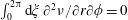 $\int _{0}^{2\unicode[STIX]{x03C0}}\text{d}\unicode[STIX]{x1D709}\;\unicode[STIX]{x2202}^{2}\unicode[STIX]{x1D708}/\unicode[STIX]{x2202}r\unicode[STIX]{x2202}\unicode[STIX]{x1D719}=0$
at
$\int _{0}^{2\unicode[STIX]{x03C0}}\text{d}\unicode[STIX]{x1D709}\;\unicode[STIX]{x2202}^{2}\unicode[STIX]{x1D708}/\unicode[STIX]{x2202}r\unicode[STIX]{x2202}\unicode[STIX]{x1D719}=0$
at
 $r=0$
. It follows that the
$r=0$
. It follows that the
 $\unicode[STIX]{x2202}{\hat{g}}/\unicode[STIX]{x2202}\unicode[STIX]{x1D719}$
has no term linear in
$\unicode[STIX]{x2202}{\hat{g}}/\unicode[STIX]{x2202}\unicode[STIX]{x1D719}$
has no term linear in
 $r$
. Then since we are free to shift
$r$
. Then since we are free to shift
 $\unicode[STIX]{x1D708}$
by any function of only
$\unicode[STIX]{x1D708}$
by any function of only
 $r$
, we can choose
$r$
, we can choose
 ${\hat{g}}$
so
${\hat{g}}$
so
 $\unicode[STIX]{x1D708}$
has the form
$\unicode[STIX]{x1D708}$
has the form
 $$\begin{eqnarray}\unicode[STIX]{x1D708}=\unicode[STIX]{x1D708}_{0}(\unicode[STIX]{x1D719})+r(\unicode[STIX]{x1D708}_{1s}^{\unicode[STIX]{x1D709}}\sin \unicode[STIX]{x1D709}+\unicode[STIX]{x1D708}_{1c}^{\unicode[STIX]{x1D709}}\cos \unicode[STIX]{x1D709})+r^{2}(\unicode[STIX]{x1D708}_{20}^{\unicode[STIX]{x1D709}}+\unicode[STIX]{x1D708}_{2s}^{\unicode[STIX]{x1D709}}\sin 2\unicode[STIX]{x1D709}+\unicode[STIX]{x1D708}_{2c}^{\unicode[STIX]{x1D709}}\cos 2\unicode[STIX]{x1D709})+O(r^{3}).\end{eqnarray}$$
Substitution of
 $\unicode[STIX]{x1D709}=\unicode[STIX]{x1D703}-\unicode[STIX]{x1D704}\unicode[STIX]{x1D708}$
and (A 17) in (A 11) yields the desired expansions for
$\unicode[STIX]{x1D709}=\unicode[STIX]{x1D703}-\unicode[STIX]{x1D704}\unicode[STIX]{x1D708}$
and (A 17) in (A 11) yields the desired expansions for
 $R$
and
$R$
and
 $z$
, equations (2.12)–(2.14). The same substitutions applied to (A 17) give the desired expansion for
$z$
, equations (2.12)–(2.14). The same substitutions applied to (A 17) give the desired expansion for
 $\unicode[STIX]{x1D708}(r,\unicode[STIX]{x1D703},\unicode[STIX]{x1D719})$
.
$\unicode[STIX]{x1D708}(r,\unicode[STIX]{x1D703},\unicode[STIX]{x1D719})$
.
Finally,
 $B$
is smooth near the axis and so it has a Taylor expansion
$B$
is smooth near the axis and so it has a Taylor expansion
 $$\begin{eqnarray}\displaystyle B & = & \displaystyle B_{0}+(R-R_{0})B_{R}+(z-z_{0})B_{z}+{\textstyle \frac{1}{2}}(R-R_{0})^{2}B_{RR}\nonumber\\ \displaystyle & & \displaystyle +\,(R-R_{0})(z-z_{0})B_{Rz}+{\textstyle \frac{1}{2}}(z-z_{0})^{2}B_{zz}+O(r^{3}).\end{eqnarray}$$
Substitution of (2.12)–(2.14) for
 $R(r,\unicode[STIX]{x1D703},\unicode[STIX]{x1D719})$
and the analogous expansion for
$R(r,\unicode[STIX]{x1D703},\unicode[STIX]{x1D719})$
and the analogous expansion for
 $z(r,\unicode[STIX]{x1D703},\unicode[STIX]{x1D719})$
into (A 18) gives the desired expansion for
$z(r,\unicode[STIX]{x1D703},\unicode[STIX]{x1D719})$
into (A 18) gives the desired expansion for
 $B(r,\unicode[STIX]{x1D703},\unicode[STIX]{x1D719})$
.
$B(r,\unicode[STIX]{x1D703},\unicode[STIX]{x1D719})$
.
Appendix B. Geometric properties of flux surfaces
Here we relate several geometric properties of the flux surfaces – specifically the cross-sectional area and elongation – to the variables
 $(R_{1},z_{1})$
used elsewhere in the paper. We consider a cross-section of the flux surfaces in a constant-
$(R_{1},z_{1})$
used elsewhere in the paper. We consider a cross-section of the flux surfaces in a constant-
 $\unicode[STIX]{x1D719}$
plane. All results of this section apply to cross-sections perpendicular to the magnetic axis if
$\unicode[STIX]{x1D719}$
plane. All results of this section apply to cross-sections perpendicular to the magnetic axis if
 $(R_{1},z_{1})$
are replaced by
$(R_{1},z_{1})$
are replaced by
 $(X_{1},Y_{1})$
. Several geometric quantities are defined in figure 2. To
$(X_{1},Y_{1})$
. Several geometric quantities are defined in figure 2. To
 $O(r)$
, the flux surfaces are elliptical, with semi-major axis
$O(r)$
, the flux surfaces are elliptical, with semi-major axis
 $a$
and semi-minor axis
$a$
and semi-minor axis
 $b$
. Axes
$b$
. Axes
 $u$
and
$u$
and
 $v$
are aligned with the minor and major axes, and
$v$
are aligned with the minor and major axes, and
 $\unicode[STIX]{x1D6FE}$
is the angle between the
$\unicode[STIX]{x1D6FE}$
is the angle between the
 $u$
and
$u$
and
 $R_{1}$
axes. The
$R_{1}$
axes. The
 $\unicode[STIX]{x1D703}=0$
line is not generally aligned with any of these axes, and we let
$\unicode[STIX]{x1D703}=0$
line is not generally aligned with any of these axes, and we let
 $\unicode[STIX]{x1D703}_{0}$
denote the angle between this line and the
$\unicode[STIX]{x1D703}_{0}$
denote the angle between this line and the
 $R_{1}$
axis. Any point in the plane, such as the black dot in the figure, makes an angle
$R_{1}$
axis. Any point in the plane, such as the black dot in the figure, makes an angle
 $\unicode[STIX]{x1D703}+\unicode[STIX]{x1D703}_{0}$
relative to the
$\unicode[STIX]{x1D703}+\unicode[STIX]{x1D703}_{0}$
relative to the
 $R_{1}$
axis and an angle
$R_{1}$
axis and an angle
 $\unicode[STIX]{x1D712}$
relative to the
$\unicode[STIX]{x1D712}$
relative to the
 $u$
axis, with
$u$
axis, with
 $\unicode[STIX]{x1D712}=\unicode[STIX]{x1D703}+\unicode[STIX]{x1D703}_{0}+\unicode[STIX]{x1D6FE}$
. Substituting
$\unicode[STIX]{x1D712}=\unicode[STIX]{x1D703}+\unicode[STIX]{x1D703}_{0}+\unicode[STIX]{x1D6FE}$
. Substituting
 $u=b\cos \unicode[STIX]{x1D712}$
and
$u=b\cos \unicode[STIX]{x1D712}$
and
 $v=a\sin \unicode[STIX]{x1D712}$
into
$v=a\sin \unicode[STIX]{x1D712}$
into
 $$\begin{eqnarray}\left(\begin{array}{@{}c@{}}R_{1}\\ z_{1}\end{array}\right)=\left(\begin{array}{@{}cc@{}}\cos \unicode[STIX]{x1D6FE} & \sin \unicode[STIX]{x1D6FE}\\ -\sin \unicode[STIX]{x1D6FE} & \cos \unicode[STIX]{x1D6FE}\end{array}\right)\left(\begin{array}{@{}c@{}}u\\ v\end{array}\right),\end{eqnarray}$$
applying the angle sum formula to
 $\unicode[STIX]{x1D712}$
and equating
$\unicode[STIX]{x1D712}$
and equating
 $\sin \unicode[STIX]{x1D703}$
and
$\sin \unicode[STIX]{x1D703}$
and
 $\cos \unicode[STIX]{x1D703}$
terms using (2.13), we find
$\cos \unicode[STIX]{x1D703}$
terms using (2.13), we find
 $$\begin{eqnarray}\left.\begin{array}{@{}c@{}}\displaystyle \left(\begin{array}{@{}c@{}}R_{1s}\\ R_{1c}\end{array}\right)=\left(\begin{array}{@{}cc@{}}\cos \unicode[STIX]{x1D703}_{0} & -\sin \unicode[STIX]{x1D703}_{0}\\ \sin \unicode[STIX]{x1D703}_{0} & \cos \unicode[STIX]{x1D703}_{0}\end{array}\right)\left(\begin{array}{@{}c@{}}(a-b)\sin \unicode[STIX]{x1D6FE}\cos \unicode[STIX]{x1D6FE}\\ a\sin ^{2}\unicode[STIX]{x1D6FE}+b\cos ^{2}\unicode[STIX]{x1D6FE}\end{array}\right),\\ \displaystyle \left(\begin{array}{@{}c@{}}z_{1s}\\ z_{1c}\end{array}\right)=\left(\begin{array}{@{}cc@{}}\cos \unicode[STIX]{x1D703}_{0} & -\sin \unicode[STIX]{x1D703}_{0}\\ \sin \unicode[STIX]{x1D703}_{0} & \cos \unicode[STIX]{x1D703}_{0}\end{array}\right)\left(\begin{array}{@{}c@{}}a\cos ^{2}\unicode[STIX]{x1D6FE}+b\sin ^{2}\unicode[STIX]{x1D6FE}\\ (a-b)\sin \unicode[STIX]{x1D6FE}\cos \unicode[STIX]{x1D6FE}\end{array}\right).\end{array}\right\}\end{eqnarray}$$
Using (B 2), the right-hand side of (2.24) is found to be
 $$\begin{eqnarray}R_{1s}z_{1c}-R_{1c}z_{1s}=-ab,\end{eqnarray}$$
which is (minus) the area of the ellipse divided by
 $\unicode[STIX]{x03C0}$
.
$\unicode[STIX]{x03C0}$
.
Definitions for appendix B.
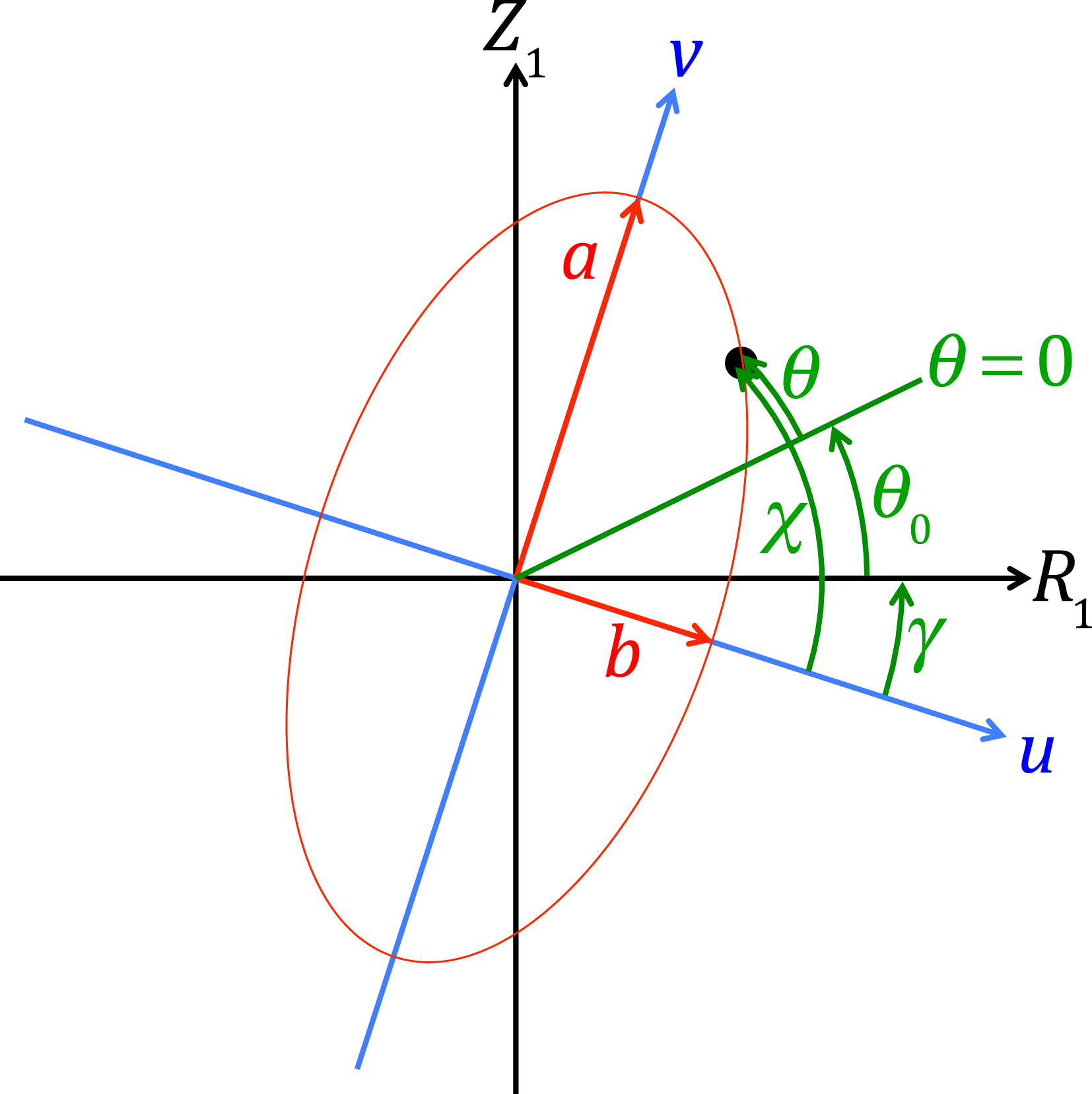
Another important property of the flux surfaces is their elongation,
 $a/b$
. In practice, many solutions of (3.13) are uninteresting since they correspond to impractically large values of elongation, so to discard these solutions it is valuable to derive an expression for the elongation in terms of
$a/b$
. In practice, many solutions of (3.13) are uninteresting since they correspond to impractically large values of elongation, so to discard these solutions it is valuable to derive an expression for the elongation in terms of
 $R_{1}$
and
$R_{1}$
and
 $z_{1}$
. Such a formula can be obtained by first defining
$z_{1}$
. Such a formula can be obtained by first defining
 $p=R_{1s}^{2}+R_{1c}^{2}+z_{1s}^{2}+z_{1c}^{2}$
, and noting from (B 2) that
$p=R_{1s}^{2}+R_{1c}^{2}+z_{1s}^{2}+z_{1c}^{2}$
, and noting from (B 2) that
 $p=a^{2}+b^{2}$
. Then defining
$p=a^{2}+b^{2}$
. Then defining
 $q=R_{1s}z_{1c}-R_{1c}z_{1s}=-ab$
, we can solve
$q=R_{1s}z_{1c}-R_{1c}z_{1s}=-ab$
, we can solve
 $a^{4}-pa^{2}+q^{2}=0$
for
$a^{4}-pa^{2}+q^{2}=0$
for
 $a$
, noting the larger positive root is
$a$
, noting the larger positive root is
 $a$
and the smaller is
$a$
and the smaller is
 $b$
, since
$b$
, since
 $b$
satisfies the same quadratic equation. Then the elongation is
$b$
satisfies the same quadratic equation. Then the elongation is
 $$\begin{eqnarray}\frac{a}{b}=\sqrt{\frac{p+\sqrt{p^{2}-4q^{2}}}{p-\sqrt{p^{2}-4q^{2}}}}=\frac{p+\sqrt{p^{2}-4q^{2}}}{2|q|}.\end{eqnarray}$$
Appendix C. Equating representations of the field: second order
Here the derivation of (2.34)–(2.36) is presented. The
 $O(r^{2})$
terms in (2.8)–(2.10) can be obtained by applying
$O(r^{2})$
terms in (2.8)–(2.10) can be obtained by applying
 $\unicode[STIX]{x2202}/\unicode[STIX]{x2202}r$
twice and evaluating the results at
$\unicode[STIX]{x2202}/\unicode[STIX]{x2202}r$
twice and evaluating the results at
 $r\rightarrow 0$
. We find
$r\rightarrow 0$
. We find
 $$\begin{eqnarray}\displaystyle & & \displaystyle \frac{\bar{B}}{G_{0}R_{0}}\left[\frac{\unicode[STIX]{x2202}R_{1}}{\unicode[STIX]{x2202}\unicode[STIX]{x1D719}}+\unicode[STIX]{x1D704}_{0}(1+\unicode[STIX]{x1D708}_{0}^{\prime })\frac{\unicode[STIX]{x2202}R_{1}}{\unicode[STIX]{x2202}\unicode[STIX]{x1D703}}-\frac{R_{1}}{R_{0}}R_{0}^{\prime }-\unicode[STIX]{x1D704}_{0}\frac{\unicode[STIX]{x2202}\unicode[STIX]{x1D708}_{1}}{\unicode[STIX]{x2202}\unicode[STIX]{x1D703}}R_{0}^{\prime }+\unicode[STIX]{x1D6FD}_{0}R_{0}\frac{\unicode[STIX]{x2202}z_{1}}{\unicode[STIX]{x2202}\unicode[STIX]{x1D703}}\right]\nonumber\\ \displaystyle & & \displaystyle \qquad =\frac{I_{2}z_{1}}{G_{0}}+\frac{\unicode[STIX]{x2202}\unicode[STIX]{x1D708}_{2}}{\unicode[STIX]{x2202}\unicode[STIX]{x1D703}}z_{1}+2\frac{\unicode[STIX]{x2202}\unicode[STIX]{x1D708}_{1}}{\unicode[STIX]{x2202}\unicode[STIX]{x1D703}}z_{2}-\unicode[STIX]{x1D708}_{1}\frac{\unicode[STIX]{x2202}z_{2}}{\unicode[STIX]{x2202}\unicode[STIX]{x1D703}}-2\unicode[STIX]{x1D708}_{2}\frac{\unicode[STIX]{x2202}z_{1}}{\unicode[STIX]{x2202}\unicode[STIX]{x1D703}},\end{eqnarray}$$
 $$\begin{eqnarray}\displaystyle & & \displaystyle \frac{\bar{B}}{G_{0}R_{0}}\left[-\frac{R_{1}}{R_{0}}(\ell ^{\prime })^{2}-\unicode[STIX]{x1D704}_{0}\frac{\unicode[STIX]{x2202}\unicode[STIX]{x1D708}_{1}}{\unicode[STIX]{x2202}\unicode[STIX]{x1D703}}(\ell ^{\prime })^{2}+2R_{0}R_{1}+2R_{0}^{\prime }\frac{\unicode[STIX]{x2202}R_{1}}{\unicode[STIX]{x2202}\unicode[STIX]{x1D719}}+2z_{0}^{\prime }\frac{\unicode[STIX]{x2202}z_{1}}{\unicode[STIX]{x2202}\unicode[STIX]{x1D719}}\right.\nonumber\\ \displaystyle & & \displaystyle \left.\qquad +\,\unicode[STIX]{x1D704}_{0}\left(1+\frac{d\unicode[STIX]{x1D708}_{0}}{d\unicode[STIX]{x1D719}}\right)\left(\frac{\unicode[STIX]{x2202}R_{1}}{\unicode[STIX]{x2202}\unicode[STIX]{x1D703}}R_{0}^{\prime }+\frac{\unicode[STIX]{x2202}z_{1}}{\unicode[STIX]{x2202}\unicode[STIX]{x1D703}}z_{0}^{\prime }\right)\right]\nonumber\\ \displaystyle & & \displaystyle \quad =\left(2z_{2}\frac{\unicode[STIX]{x2202}R_{1}}{\unicode[STIX]{x2202}\unicode[STIX]{x1D703}}+z_{1}\frac{\unicode[STIX]{x2202}R_{2}}{\unicode[STIX]{x2202}\unicode[STIX]{x1D703}}-2R_{2}\frac{\unicode[STIX]{x2202}z_{1}}{\unicode[STIX]{x2202}\unicode[STIX]{x1D703}}-R_{1}\frac{\unicode[STIX]{x2202}z_{2}}{\unicode[STIX]{x2202}\unicode[STIX]{x1D703}}\right)(1+\unicode[STIX]{x1D708}_{0}^{\prime })\nonumber\\ \displaystyle & & \displaystyle \qquad +\,\left(z_{1}\frac{\unicode[STIX]{x2202}R_{1}}{\unicode[STIX]{x2202}\unicode[STIX]{x1D703}}-R_{1}\frac{\unicode[STIX]{x2202}z_{1}}{\unicode[STIX]{x2202}\unicode[STIX]{x1D703}}\right)\frac{\unicode[STIX]{x2202}\unicode[STIX]{x1D708}_{1}}{\unicode[STIX]{x2202}\unicode[STIX]{x1D719}},\end{eqnarray}$$
 $$\begin{eqnarray}\displaystyle & & \displaystyle \frac{\bar{B}}{G_{0}R_{0}}\left[\frac{\unicode[STIX]{x2202}z_{1}}{\unicode[STIX]{x2202}\unicode[STIX]{x1D719}}+\unicode[STIX]{x1D704}_{0}(1+\unicode[STIX]{x1D708}_{0}^{\prime })\frac{\unicode[STIX]{x2202}z_{1}}{\unicode[STIX]{x2202}\unicode[STIX]{x1D703}}-\frac{R_{1}}{R_{0}}z_{0}^{\prime }-\unicode[STIX]{x1D704}_{0}\frac{\unicode[STIX]{x2202}\unicode[STIX]{x1D708}_{1}}{\unicode[STIX]{x2202}\unicode[STIX]{x1D703}}z_{0}^{\prime }-\unicode[STIX]{x1D6FD}_{0}R_{0}\frac{\unicode[STIX]{x2202}R_{1}}{\unicode[STIX]{x2202}\unicode[STIX]{x1D703}}\right]\nonumber\\ \displaystyle & & \displaystyle \quad =-\frac{I_{2}R_{1}}{G_{0}}+\frac{\unicode[STIX]{x2202}R_{2}}{\unicode[STIX]{x2202}\unicode[STIX]{x1D703}}\unicode[STIX]{x1D708}_{1}+2\frac{\unicode[STIX]{x2202}R_{1}}{\unicode[STIX]{x2202}\unicode[STIX]{x1D703}}\unicode[STIX]{x1D708}_{2}-R_{1}\frac{\unicode[STIX]{x2202}\unicode[STIX]{x1D708}_{2}}{\unicode[STIX]{x2202}\unicode[STIX]{x1D703}}-2R_{2}\frac{\unicode[STIX]{x2202}\unicode[STIX]{x1D708}_{1}}{\unicode[STIX]{x2202}\unicode[STIX]{x1D703}}.\end{eqnarray}$$
In (C 2), the terms including a factor of
 $\unicode[STIX]{x1D704}_{0}$
can be written in the combination (2.29), which vanishes as before. Plugging in (2.13)–(2.14), it can be seen that (C 1)–(C 3) each have only
$\unicode[STIX]{x1D704}_{0}$
can be written in the combination (2.29), which vanishes as before. Plugging in (2.13)–(2.14), it can be seen that (C 1)–(C 3) each have only
 $\sin \unicode[STIX]{x1D703}$
and
$\sin \unicode[STIX]{x1D703}$
and
 $\cos \unicode[STIX]{x1D703}$
Fourier components. These
$\cos \unicode[STIX]{x1D703}$
Fourier components. These
 $\sin \unicode[STIX]{x1D703}$
and
$\sin \unicode[STIX]{x1D703}$
and
 $\cos \unicode[STIX]{x1D703}$
components give the following six equations:
$\cos \unicode[STIX]{x1D703}$
components give the following six equations:
 $$\begin{eqnarray}\displaystyle & & \displaystyle \frac{\bar{B}}{2G_{0}R_{0}}\left[R_{1s}^{\prime }-\unicode[STIX]{x1D704}_{0}(1+\unicode[STIX]{x1D708}_{0}^{\prime })R_{1c}-\frac{R_{1s}}{R_{0}}R_{0}^{\prime }+\unicode[STIX]{x1D704}_{0}\unicode[STIX]{x1D708}_{1c}R_{0}^{\prime }-\unicode[STIX]{x1D6FD}_{0}R_{0}z_{1c}\right]\nonumber\\ \displaystyle & & \displaystyle \quad =\frac{I_{2}z_{1s}}{2G_{0}}+\unicode[STIX]{x1D708}_{1c}(z_{2c}-z_{20})+\unicode[STIX]{x1D708}_{1s}z_{2s}+z_{1c}(\unicode[STIX]{x1D708}_{20}-\unicode[STIX]{x1D708}_{2c})-z_{1s}\unicode[STIX]{x1D708}_{2s},\end{eqnarray}$$
 $$\begin{eqnarray}\displaystyle & & \displaystyle \frac{\bar{B}}{2G_{0}R_{0}}\left[R_{1c}^{\prime }+\unicode[STIX]{x1D704}_{0}(1+\unicode[STIX]{x1D708}_{0}^{\prime })R_{1s}-\frac{R_{1c}}{R_{0}}R_{0}^{\prime }-\unicode[STIX]{x1D704}_{0}\unicode[STIX]{x1D708}_{1s}R_{0}^{\prime }+\unicode[STIX]{x1D6FD}_{0}R_{0}z_{1s}\right]\nonumber\\ \displaystyle & & \displaystyle \quad =\frac{I_{2}z_{1c}}{2G_{0}}+\unicode[STIX]{x1D708}_{1s}(z_{2c}+z_{20})-\unicode[STIX]{x1D708}_{1c}z_{2s}-z_{1s}(\unicode[STIX]{x1D708}_{20}+\unicode[STIX]{x1D708}_{2c})+z_{1c}\unicode[STIX]{x1D708}_{2s},\end{eqnarray}$$
 $$\begin{eqnarray}\displaystyle & & \displaystyle \frac{\bar{B}}{2G_{0}R_{0}}\left[z_{1s}^{\prime }-\unicode[STIX]{x1D704}_{0}(1+\unicode[STIX]{x1D708}_{0}^{\prime })z_{1c}-\frac{R_{1s}}{R_{0}}z_{0}^{\prime }+\unicode[STIX]{x1D704}_{0}\unicode[STIX]{x1D708}_{1c}z_{0}^{\prime }+\unicode[STIX]{x1D6FD}_{0}R_{0}R_{1c}\right]\nonumber\\ \displaystyle & & \displaystyle \quad =-\frac{I_{2}R_{1s}}{2G_{0}}+\unicode[STIX]{x1D708}_{1c}(R_{20}-R_{2c})-\unicode[STIX]{x1D708}_{1s}R_{2s}+R_{1c}(\unicode[STIX]{x1D708}_{2c}-\unicode[STIX]{x1D708}_{20})+R_{1s}\unicode[STIX]{x1D708}_{2s},\end{eqnarray}$$
 $$\begin{eqnarray}\displaystyle & & \displaystyle \frac{\bar{B}}{2G_{0}R_{0}}\left[z_{1c}^{\prime }+\unicode[STIX]{x1D704}_{0}(1+\unicode[STIX]{x1D708}_{0}^{\prime })z_{1s}-\frac{R_{1c}}{R_{0}}z_{0}^{\prime }-\unicode[STIX]{x1D704}_{0}\unicode[STIX]{x1D708}_{1s}z_{0}^{\prime }-\unicode[STIX]{x1D6FD}_{0}R_{0}R_{1s}\right]\nonumber\\ \displaystyle & & \displaystyle \quad =-\frac{I_{2}R_{c1}}{2G_{0}}-\unicode[STIX]{x1D708}_{1s}\left(R_{20}+R_{2c}\right)+\unicode[STIX]{x1D708}_{1c}R_{2s}+R_{1s}\left(\unicode[STIX]{x1D708}_{2c}+\unicode[STIX]{x1D708}_{20}\right)-R_{1c}\unicode[STIX]{x1D708}_{2s},\end{eqnarray}$$
 $$\begin{eqnarray}\displaystyle & & \displaystyle \frac{\bar{B}}{G_{0}R_{0}}\left[-\frac{R_{1s}}{2R_{0}}(\ell ^{\prime })^{2}+R_{0}R_{1s}+R_{0}^{\prime }R_{1s}^{\prime }+z_{0}^{\prime }z_{1s}^{\prime }\right]\nonumber\\ \displaystyle & & \displaystyle \quad =\left[z_{1c}(R_{20}-R_{2c})-z_{1s}R_{2s}+R_{1c}(z_{2c}-z_{20})+R_{1s}z_{2s}\right](1+\unicode[STIX]{x1D708}_{0}^{\prime })+\frac{s_{G}\bar{B}}{2R_{0}B_{0}}\ell ^{\prime }\unicode[STIX]{x1D708}_{1s}^{\prime },\nonumber\\ \displaystyle & & \displaystyle\end{eqnarray}$$
 $$\begin{eqnarray}\displaystyle & & \displaystyle \frac{\bar{B}}{G_{0}R_{0}}\left[-\frac{R_{1c}}{2R_{0}}(\ell ^{\prime })^{2}+R_{0}R_{1c}+R_{0}^{\prime }R_{1c}^{\prime }+z_{0}^{\prime }z_{1c}^{\prime }\right]\nonumber\\ \displaystyle & & \displaystyle \quad =[-z_{1s}(R_{2c}+R_{20})+z_{1c}R_{2s}+R_{1s}(z_{20}+z_{2c})-R_{1c}z_{2s}](1+\unicode[STIX]{x1D708}_{0}^{\prime })+\frac{s_{G}\bar{B}}{2R_{0}B_{0}}\ell ^{\prime }\unicode[STIX]{x1D708}_{1c}^{\prime }.\nonumber\\ \displaystyle & & \displaystyle\end{eqnarray}$$
In the last two equations we have used (2.24).
While these six equations contain
 $R_{2}$
,
$R_{2}$
,
 $\unicode[STIX]{x1D708}_{2}$
and
$\unicode[STIX]{x1D708}_{2}$
and
 $z_{2}$
, all these subscript-2 quantities can be eliminated to give a constraint on the subscript-1 quantities by forming
$z_{2}$
, all these subscript-2 quantities can be eliminated to give a constraint on the subscript-1 quantities by forming
 $$\begin{eqnarray}(1+\unicode[STIX]{x1D708}_{0}^{\prime })[\text{(C4)}R_{1c}-\text{(C5)}R_{1s}+\text{(C6)}z_{1c}-\text{(C7)}z_{1s}]-\text{(C8)}\unicode[STIX]{x1D708}_{1c}+\text{(C9)}\unicode[STIX]{x1D708}_{1s}.\end{eqnarray}$$
The
 $\unicode[STIX]{x1D6FD}_{0}$
terms happen to vanish as well in this combination. Multiplying the result through by
$\unicode[STIX]{x1D6FD}_{0}$
terms happen to vanish as well in this combination. Multiplying the result through by
 $2G_{0}R_{0}/\bar{B}$
, we obtain
$2G_{0}R_{0}/\bar{B}$
, we obtain
 $$\begin{eqnarray}\displaystyle & & \displaystyle (1+\unicode[STIX]{x1D708}_{0}^{\prime })\left[R_{1c}R_{1s}^{\prime }-R_{1s}R_{1c}^{\prime }+z_{1c}z_{1s}^{\prime }-z_{1s}z_{1c}^{\prime }+(R_{1c}z_{1s}-R_{1s}z_{1c})z_{0}^{\prime }/R_{0}\right.\nonumber\\ \displaystyle & & \displaystyle \qquad -\,\unicode[STIX]{x1D704}_{0}(1+\unicode[STIX]{x1D708}_{0}^{\prime })(R_{1c}^{2}+R_{1s}^{2}+z_{1c}^{2}+z_{1s}^{2})\nonumber\\ \displaystyle & & \displaystyle \qquad \left.+\,\unicode[STIX]{x1D704}_{0}R_{0}^{\prime }(\unicode[STIX]{x1D708}_{1c}R_{1c}+\unicode[STIX]{x1D708}_{1s}R_{1s})+\unicode[STIX]{x1D704}_{0}z_{0}^{\prime }(\unicode[STIX]{x1D708}_{1c}z_{1c}+\unicode[STIX]{x1D708}_{1s}z_{1s})\right]\nonumber\\ \displaystyle & & \displaystyle \qquad -\,2\unicode[STIX]{x1D708}_{1c}\left[-\frac{R_{1s}}{2R_{0}}(\ell ^{\prime })^{2}+R_{0}R_{1s}+R_{0}^{\prime }R_{1s}^{\prime }+z_{0}^{\prime }z_{1s}^{\prime }\right]\nonumber\\ \displaystyle & & \displaystyle \qquad +\,2\unicode[STIX]{x1D708}_{1s}\left[-\frac{R_{1c}}{2R_{0}}(\ell ^{\prime })^{2}+R_{0}R_{1c}+R_{0}^{\prime }R_{1c}^{\prime }+z_{0}^{\prime }z_{1c}^{\prime }\right]\nonumber\\ \displaystyle & & \displaystyle \quad =\frac{|G_{0}|}{B_{0}}\ell ^{\prime }(\unicode[STIX]{x1D708}_{1s}\unicode[STIX]{x1D708}_{1c}^{\prime }-\unicode[STIX]{x1D708}_{1c}\unicode[STIX]{x1D708}_{1s}^{\prime })+\frac{2I_{2}R_{0}}{\bar{B}}(1+\unicode[STIX]{x1D708}_{0}^{\prime })(R_{1c}z_{1s}-R_{1s}z_{1c}).\end{eqnarray}$$
Eliminating
 $\unicode[STIX]{x1D708}_{0}$
, we find
$\unicode[STIX]{x1D708}_{0}$
, we find
 $(T-\unicode[STIX]{x1D704}_{0}V)(\ell ^{\prime })^{2}B_{0}^{2}/G_{0}^{2}=0$
where
$(T-\unicode[STIX]{x1D704}_{0}V)(\ell ^{\prime })^{2}B_{0}^{2}/G_{0}^{2}=0$
where
 $$\begin{eqnarray}\displaystyle T & = & \displaystyle \frac{|G_{0}|^{3}}{B_{0}^{3}\ell ^{\prime }}(\unicode[STIX]{x1D708}_{1c}\unicode[STIX]{x1D708}_{1s}^{\prime }-\unicode[STIX]{x1D708}_{1s}\unicode[STIX]{x1D708}_{1c}^{\prime })\nonumber\\ \displaystyle & & \displaystyle +\,\frac{|G_{0}|}{B_{0}\ell ^{\prime }}\left[R_{1c}R_{1s}^{\prime }-R_{1s}R_{1c}^{\prime }+z_{1c}z_{1s}^{\prime }-z_{1s}z_{1c}^{\prime }+\frac{(R_{1c}z_{1s}-R_{1s}z_{1c})}{R_{0}}z_{0}^{\prime }\right]\nonumber\\ \displaystyle & & \displaystyle -\,\frac{2G_{0}^{2}\unicode[STIX]{x1D708}_{1c}}{B_{0}^{2}(\ell ^{\prime })^{2}}\left[-\frac{R_{1s}}{2R_{0}}(\ell ^{\prime })^{2}+R_{0}R_{1s}+R_{0}^{\prime }R_{1s}^{\prime }+z_{0}^{\prime }z_{1s}^{\prime }\right]\nonumber\\ \displaystyle & & \displaystyle +\,\frac{2G_{0}^{2}\unicode[STIX]{x1D708}_{1s}}{B_{0}^{2}(\ell ^{\prime })^{2}}\left[-\frac{R_{1c}}{2R_{0}}(\ell ^{\prime })^{2}+R_{0}R_{1c}+R_{0}^{\prime }R_{1c}^{\prime }+z_{0}^{\prime }z_{1c}^{\prime }\right]+\frac{2I_{2}G_{0}}{B_{0}^{2}},\end{eqnarray}$$
and
 $$\begin{eqnarray}V=R_{1c}^{2}+R_{1s}^{2}+z_{1c}^{2}+z_{1s}^{2}-\frac{|G_{0}|}{B_{0}\ell ^{\prime }}[R_{0}^{\prime }(\unicode[STIX]{x1D708}_{1c}R_{1c}+\unicode[STIX]{x1D708}_{1s}R_{1s})+z_{0}^{\prime }(\unicode[STIX]{x1D708}_{1c}z_{1c}+\unicode[STIX]{x1D708}_{1s}z_{1s})].\end{eqnarray}$$
Eliminating
 $\unicode[STIX]{x1D708}_{1s}$
and
$\unicode[STIX]{x1D708}_{1s}$
and
 $\unicode[STIX]{x1D708}_{1c}$
using (2.27) results in (2.35)–(2.36).
$\unicode[STIX]{x1D708}_{1c}$
using (2.27) results in (2.35)–(2.36).


