


1. Introduction
Flow in fractures is a situation widely encountered in practical applications such as the leakage rate of seals (e.g. Pérez-Ràfols, Larsson & Almqvist Reference Pérez-Ràfols, Larsson and Almqvist2016; Rui et al. Reference Rui, Wei, Hehua, Yaji, Rui and Xinbin2023), gas leak through reservoir caps or gas recovery in fractured rocks (see Zhou et al. (Reference Zhou, Chen, Hu and Yang2023) and references therein), among many others. Modelling flow in rough fractures has been carried out using the average Reynolds equations over several decades. In early works, surface roughness was treated as a stochastic variable in one dimension (Tzeng & Saibel Reference Tzeng and Saibel1967); however, in the work by Patir & Cheng (Reference Patir and Cheng1978), an average Reynolds equation was proposed in terms of the macroscopic pressure gradient and shear flow factors, thus making it possible to handle three-dimensional fractures. Using the volume averaging method, Prat, Plouraboué & Letalleur (Reference Prat, Plouraboué and Letalleur2002) later showed that these factors were predictable from closure problem solutions in a representative periodic unit cell.
While many studies of flow through rough fractures have adopted no-slip boundary conditions at the solid–fluid interface, this assumption is not always justified in situations of practical interest such as non-wetting fluid flow (Lee, Yo & Lee Reference Lee, Yo and Lee2013) or rarefied gas flow (Wang, Tang & Jing Reference Wang, Tang and Jing2019). In the slip regime, characterised by a Knudsen number (i.e. the ratio of the gas molecules mean-free path to a characteristic constriction length) smaller than  ${\sim }0.1$, gas flow can be modelled, at the local scale, with the Reynolds (lubrication) equation that includes gas slippage effects at the walls (Zaouter, Lasseux & Prat Reference Zaouter, Lasseux and Prat2018). The same type of model operates as well for slip mechanisms different from Knudsen effects.
Since fractures often exhibit a roughness that is multiscale in nature, upscaled flow models are favoured in practice. Such models also have a Reynolds-like form involving the macroscopic effective transmissivity tensor that lumps the geometrical and slip effects. To separate the latter from the pure viscous contribution, a Knudsen number power-series expansion can be performed, which provides the intrinsic transmissivity tensor as well as a series of intrinsic correction tensors at multiple orders. These tensors can be considered to be intrinsic as they only depend on the fracture geometry. They can be computed from solving a set of sequentially coupled ancillary closure problems on a periodic unit cell representative of the system under consideration. These problems can be relatively difficult to solve and computationally costly, and the sequential coupling is prone to the propagation of numerical errors in the solutions at the successive orders. Moreover, the use of power-series expansions does not necessarily guarantee convergence and this poses a serious problem in terms of accuracy.
To address this issue, a procedure is derived that considerably simplifies the determination of the successive correction tensors as the solution of the first  $N$ closure problems provides the correction tensors up to the $2N-1$ order. The analysis allows determination of the symmetry and definiteness properties of the individual tensors. In addition, it is shown that the power-series expansion can be employed to form a Padé approximant, which, in its simplest form, is built using the first three correction tensors, that are obtained from the solution of only the first two ancillary closure problems.
The article is organised as follows. In § 2, the local and macroscale models derived in Zaouter et al. (Reference Zaouter, Lasseux and Prat2018) for gas slip flow in a rough fracture are recalled. In addition, the associated closure problems resulting from power-series expansions in the Knudsen number are presented. In § 3, an integral approach is used to express the correction tensors at the different orders in the Knudsen number, showing that the computational requirements are reduced by a factor of almost two. The analysis also provides the proof of symmetry and semi-positive definiteness of the tensors. In addition, a Padé approximant is constructed requiring the minimum number of correction tensors to provide an alternative estimate of the effective transmissivity tensor. In § 4, numerical examples are used to validate the method derived here and illustrate the dependence of the transmissivity on the average Knudsen number, considering random rough fractures. The performance of the first-order (i.e. Klinkenberg) and higher-order corrections is explored. The Padé approximant is shown to outperform the predictions from the original power-series expansion. Finally, conclusions are presented in § 5.
2. Reynolds models at the local and macroscopic scales
The developments that follow are carried out considering the (slightly) compressible, isothermal, Newtonian and steady creeping flow of a gas within a fracture, assuming that Knudsen effects may be significant but in a rarefied regime corresponding to slip flow. Nevertheless, generalisation to slip flow in a broader context is straightforward, as it would require assuming a diffuse reflection at the solid–fluid interfaces and replacing the Knudsen number by the slip length to characteristic aperture size ratio (Bolaños & Vernescu Reference Bolaños and Vernescu2017).
2.1. Local description
Derivation of the local Reynolds equation for flow in a rough fracture in the presence of slip was carried out in a previous work (see § 2 in Zaouter et al. Reference Zaouter, Lasseux and Prat2018). The flow model at the roughness scale can be written in the following form:
 $$\begin{gather} \boldsymbol{\nabla} \boldsymbol{\cdot}\boldsymbol{q} = 0, \quad \text{in}\ \mathscr{A}_\beta, \end{gather}$$
 $$\begin{gather}\boldsymbol{q} ={-}\rho\frac{h^3}{12\mu} \left(1 + 6\xi \frac{\lambda}{h} \right) \boldsymbol{\nabla} p, \quad \text{in}\ \mathscr{A}_\beta, \end{gather}$$
 $$\begin{gather}\rho = \varphi (p), \quad \text{in}\ \mathscr{A}_\beta, \end{gather}$$
 $$\begin{gather}\boldsymbol{q} \boldsymbol{\cdot} \boldsymbol{n} = 0, \quad \text{at}\ \mathscr{C}_{\beta \sigma}. \end{gather}$$
 In the above equations,  $\boldsymbol {q}$ denotes the local mass flow rate per unit width of the fracture, and can be referred to as the local mass flux. In (2.1b), $h = h(x, y)$ represents the local aperture at a point $(x, y)$ in the mid-plane of the fracture (see figure 1) where the pressure is $p$, the density is $\rho$ and the mean-free path is $\lambda$, $\mu$ being the dynamic fluid viscosity, that is assumed constant. In addition, $\xi = (2 - \sigma _v) / \sigma _v$ is a parameter that accounts for the molecular reflection process at the solid–fluid interfaces, $\sigma _v$ being the tangential momentum accommodation coefficient (Maxwell Reference Maxwell1879). Moreover, $\mathscr {A}_\beta$ represents the portion of the fracture that is occupied by the fluid phase, $\beta$, and $\mathscr {C}_{\beta \sigma }$ denotes the contours of the solid contact zones, $\sigma$ (where $h = 0$), that are eventually present between the two rough surfaces forming the fracture (see figure 1). The state equation, (2.1c) relates the density only to the fluid pressure, under the assumption of isothermal conditions. To arrive at this flow model, it is assumed that the roughness at both walls is slowly varying. This means that the slope of the two surfaces is everywhere small compared with unity, i.e. that $\varepsilon = h_\beta / \ell _\beta \ll 1$, $h_\beta$ being the characteristic aperture size and $\ell _\beta$ the characteristic length scale in the $x$- and $y$-directions of the fracture over which $h_\beta$ varies significantly. The model is $O(\varepsilon ^2 (1 + \xi Kn) )$ accurate and its use is constrained by the Knudsen number, $\textit {Kn} = \lambda / h_\beta \lesssim 0.1$.
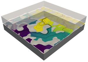
Top: sketch of the system consisting of a fracture between two rough surfaces. Note that  $h(x, y)$ represents the local aperture at any point in the mid-plane of the fracture. Bottom left: top view of part of the fracture. Bottom right: detail of the two-dimensional domain in which the Reynolds model applies, including the corresponding phases and characteristic lengths, the periodic unit cell, the axes and the notations.

2.2. Macroscopic model
The Reynolds model given in (2.1) operates locally in the two-dimensional domain corresponding to the mid-plane of the fracture. A macroscopic description over a representative element of the fracture is nevertheless of major interest and was developed in Zaouter et al. (Reference Zaouter, Lasseux and Prat2018) (cf. § 3). Under the assumption of a separation of length scales, i.e.  $\ell _\beta \ll L$, $L$ being the size of the system, it is given by
 $$\begin{gather} \boldsymbol{\nabla} \boldsymbol{\cdot} \langle\boldsymbol{q}\rangle = 0, \end{gather}$$
 $$\begin{gather}\langle\boldsymbol{q}\rangle ={-}\langle\rho\rangle^\beta\frac{{{\boldsymbol{\mathsf{K}}}}}{\mu}\boldsymbol{\cdot}\boldsymbol{\nabla}\langle p\rangle^\beta , \end{gather}$$
 $$\begin{gather}\langle\rho\rangle^\beta = \varphi ( \langle p \rangle^\beta ). \end{gather}$$
 In this model, the superficial and intrinsic surface averages of a variable,  $\psi$, taking values in $\mathscr {A}_\beta$ are respectively defined as
 $$\begin{gather} \langle\psi\rangle = \frac{1}{A}\int_{\mathscr{A}_\beta}\psi\, {\rm d} A, \end{gather}$$
 $$\begin{gather}\langle\psi\rangle^\beta = \frac{1}{A_\beta} \int_{\mathscr{A}_\beta}\psi\, {\rm d} A. \end{gather}$$
In these definitions,  $A$ and $A_\beta$ are the areas of $\mathscr {A}$ and $\mathscr {A}_\beta$, respectively, $\mathscr {A}$ being the averaging surface identified as the representative (periodic) unit cell of the fracture aperture field, and $\mathscr {A}_\beta$ the portion of $\mathscr {A}$ occupied by the $\beta$-phase, i.e. where $h \ne 0$ (cf. figure 1). Equation (2.2c) is the formal state equation at the macroscopic scale that follows from (2.1c). The above macroscopic model is obtained assuming a slightly compressible flow characterised by $\rho -\langle \rho \rangle ^\beta \ll \langle \rho \rangle ^\beta$. In the momentum equation (2.2b), ${{\boldsymbol{\mathsf{K}}}}$ is the apparent (effective) transmissivity tensor that is obtained from the solution of the following closure problem in a periodic (two-dimensional) unit cell:
 $$\begin{gather} \boldsymbol{\nabla} \boldsymbol{\cdot} (k (\boldsymbol{\nabla} \boldsymbol{b}+{{\boldsymbol{\mathsf{I}}}}))=\boldsymbol{0}, \quad \text{in } \mathscr A_\beta, \end{gather}$$
 $$\begin{gather}\boldsymbol{n} \boldsymbol{\cdot} k (\boldsymbol{\nabla} \boldsymbol{b}+{{\boldsymbol{\mathsf{I}}}})= \boldsymbol{0}, \quad \text{at } \mathscr C_{\beta \sigma}, \end{gather}$$
 $$\begin{gather}\boldsymbol{b} (\boldsymbol{r}+\boldsymbol{l}_i)= \boldsymbol{b} (\boldsymbol{r}), \quad i=1,2, \end{gather}$$
 $$\begin{gather}{{\boldsymbol{\mathsf{K}}}}=\langle k (\boldsymbol{\nabla} \boldsymbol{b}+{{\boldsymbol{\mathsf{I}}}})\rangle. \end{gather}$$
Here, the local transmissivity  $k$ is defined as
 \begin{equation} k = k_0 + \alpha k_1, \quad k_0 = \frac{h^3}{12}, \quad k_1 = \frac{h^2}{12}, \quad \alpha = 6\xi\bar{\lambda}, \end{equation}
and  $\bar {\lambda }$ is the mean-free path corresponding to the average density, $\langle \rho \rangle ^\beta$. Note that $\xi \bar {\lambda }$ can be identified as the slip length in the general case, beyond the context of gas flow in the presence of Knudsen effects. Moreover, ${{\boldsymbol{\mathsf{I}}}}$ is the identity tensor, and in (2.4c), $\boldsymbol {l}_i$ represents the lattice vector of the two-dimensional unit cell in the $i$th-direction (i.e. $\boldsymbol {l}_1 = \ell _x \boldsymbol {e}_x$, $\boldsymbol {l}_2 = \ell _y \boldsymbol {e}_y$, $(\boldsymbol {e}_x,\boldsymbol {e}_y)$ forming the system of coordinates in the plane of the fracture, see figure 1). Note that the problem defined in (2.4) may appear as ill posed since $\boldsymbol {b}$ is defined to within an additive constant. However, from (2.4d), it is clear that this constant plays no role in the prediction of ${{\boldsymbol{\mathsf{K}}}}$ and, hence, it is not required to specify it. The field of $\boldsymbol {b}$, compliant with the closure procedure, is nevertheless constrained by $\langle \boldsymbol {b}\rangle ^\beta =\boldsymbol {0}$.
The second-order effective transmissivity tensor,  ${{\boldsymbol{\mathsf{K}}}}$, is apparent (i.e. non-intrinsic) in the sense that it depends on the flow characteristic through $\bar {\lambda }$. This means that if one is interested in studying the dependence of ${{\boldsymbol{\mathsf{K}}}}$ on $\bar {\lambda }$, it is necessary to solve the boundary-value problem given in (2.4) for any value of this parameter. To elucidate this dependence, $\boldsymbol {b}$ can be expanded in power series of $\overline {Kn} = \bar {\lambda }/h_\beta$, which, in dimensional form, translates into $\boldsymbol {b} = \sum _{j=0}^m \alpha ^j \boldsymbol {b}_j$. Accordingly, the power-series expansion, $\hat {{{\boldsymbol{\mathsf{K}}}}}_m$, of ${{\boldsymbol{\mathsf{K}}}}$ at the $m$th-order in $\overline {Kn}$, is obtained as
 \begin{equation} \hat{{{\boldsymbol{\mathsf{K}}}}}_m = \sum_{j=0}^m \alpha^j{{\boldsymbol{\mathsf{K}}}}_j.\end{equation}
 Note that, although the flux to force linearity is preserved during the averaging procedure, the linearity between  ${\boldsymbol{\mathsf{K}}}$ and $\xi \bar {\lambda }$ does not persist, in general, due to the disordered nature of the fracture aperture field that is captured in the upscaling process. For this reason, it is relevant to consider the above expansion beyond the first order. Nevertheless, the use of a power-series expansion, as expressed in (2.6), although of practical value, shall be considered with caution regarding the radius of convergence with respect to $\overline {Kn}$. A thorough analysis of this convergence criterion, which may depend on the fracture aperture field, is certainly of utmost importance but goes beyond the scope of the present work. To circumvent this issue, the correction tensors series can be used to build a Padé approximant as will be detailed in § 3.5.
With the above expansions, the second-order tensors,  ${{\boldsymbol{\mathsf{K}}}}_j$ for $j\ge 0$, are obtained from the solution of the closure problem at the corresponding order given by
Order  $j = 0$
 $$\begin{gather} \boldsymbol{\nabla} \boldsymbol{\cdot} (k_0 (\boldsymbol{\nabla} \boldsymbol{b}_0+{{\boldsymbol{\mathsf{I}}}}))=\boldsymbol{0}, \quad \text{in } \mathscr A_\beta, \end{gather}$$
 $$\begin{gather}\boldsymbol{n} \boldsymbol{\cdot} k_0 (\boldsymbol{\nabla} \boldsymbol{b}_0+{{\boldsymbol{\mathsf{I}}}})= \boldsymbol{0}, \quad \text{at } \mathscr C_{\beta \sigma}, \end{gather}$$
 $$\begin{gather}\boldsymbol{b}_0 (\boldsymbol{r}+\boldsymbol{l}_i)= \boldsymbol{b}_0 (\boldsymbol{r}), \quad i=1,2, \end{gather}$$
 $$\begin{gather}{{\boldsymbol{\mathsf{K}}}}_0=\langle k_0 (\boldsymbol{\nabla} \boldsymbol{b}_0+{{\boldsymbol{\mathsf{I}}}})\rangle. \end{gather}$$
Order  $j\ge 1$
 $$\begin{gather} \boldsymbol{\nabla} \boldsymbol{\cdot} (k_0 \boldsymbol{\nabla} \boldsymbol{b}_j+ k_1 ( \boldsymbol{\nabla} \boldsymbol{b}_{j-1}+\delta_{j1}^K {{\boldsymbol{\mathsf{I}}}}))=\boldsymbol{0}, \quad \text{in } \mathscr A_\beta, \end{gather}$$
 $$\begin{gather}\boldsymbol{n} \boldsymbol{\cdot} (k_0 \boldsymbol{\nabla} \boldsymbol{b}_j+ k_1 ( \boldsymbol{\nabla} \boldsymbol{b}_{j-1} +\delta_{j1}^K {{\boldsymbol{\mathsf{I}}}}))= \boldsymbol{0}, \quad \text{at } \mathscr C_{\beta \sigma}, \end{gather}$$
 $$\begin{gather}\boldsymbol{b}_j (\boldsymbol{r}+\boldsymbol{l}_i)= \boldsymbol{b}_j (\boldsymbol{r}), \quad i=1,2, \end{gather}$$
 $$\begin{gather}{{\boldsymbol{\mathsf{K}}}}_j=\langle k_0 \boldsymbol{\nabla} \boldsymbol{b}_j+ k_1 ( \boldsymbol{\nabla} \boldsymbol{b}_{j-1}+\delta_{j1}^K {{\boldsymbol{\mathsf{I}}}})\rangle. \end{gather}$$
In (2.8),  $\delta _{j1}^K$ represents the Kronecker delta. As in the problem for $\boldsymbol {b}$, no constraint is assigned for $\boldsymbol {b}_j$, which is hence defined to within an arbitrary additive constant that has no influence on ${{\boldsymbol{\mathsf{K}}}}_j$.
It must be noted that the zeroth-order problem yields the intrinsic transmissivity tensor that is the only relevant effective coefficient at the macroscale in the absence of slip. The successive orders  $j \ge 1$ provide the effective correction tensors due to slip effects. Conversely to ${{\boldsymbol{\mathsf{K}}}}$, the tensors ${{\boldsymbol{\mathsf{K}}}}_0$, ${{\boldsymbol{\mathsf{K}}}}_1$, …, are all intrinsic to the fracture under consideration as they only depend on its aperture field, making $\hat {{\boldsymbol{\mathsf{K}}}}_m$ fully predictive. Moreover, they allow distinguishing of the contributions from slip effects from purely viscous effects. In particular, at the first order in $\overline {Kn}$, the correction leads to the Klinkenberg relationship when the gas can be considered as ideal (see end of § 3, p. 429 in Zaouter et al. Reference Zaouter, Lasseux and Prat2018), similar to the classical correction to Darcy's law in the context of slip flow in porous media (Lasseux et al. Reference Lasseux, Valdés-Parada, Ochoa-Tapia and Goyeau2014; Lasseux, Valdés-Parada & Porter Reference Lasseux, Valdés-Parada and Porter2016).
From the above expansion in  $\overline {Kn}$, it appears that the determination of the $j$th-order correction tensor requires the solution of the series of $j+1$ problems (from order $0$ to $j$). This can be extremely costly in terms of computational time and resources to achieve enough accuracy, in particular because the closure problem at order $j$ involves the gradient of the solution at the $j-1$ order, hence contributing to a propagation of errors detrimental to the final solution. This motivates exploring of simplifications in the procedure to obtain the correction tensors, which are presented in the following section. The approach is based upon an integral formula, that results from the divergence theorem, which is used recursively to express ${{\boldsymbol{\mathsf{K}}}}_{2N-1}$ in terms of the first $N$ closure problems solution. Moreover, this approach allows determination of the symmetry and definiteness properties of the correction tensors in a very simple way. In addition, the use of a simple Padé approximant is explored, that only requires the solution of the first two closure problems.
3. An efficient procedure to obtain the correction tensors  ${{\boldsymbol{\mathsf{K}}}}_j$, $j\ge 1$


3.1. Integral formula
In order to progress towards a simplified method of determining  ${{\boldsymbol{\mathsf{K}}}}_j$, it is of interest to derive an integral formula that will be extensively used in the following. Consider an arbitrary second-order tensor field, ${{\boldsymbol{\mathsf{A}}}}$, and a vector field $\boldsymbol {a}$ defined in a domain $\varOmega _\beta$ of boundary $\partial \varOmega _\beta$ and having sufficient regularity. On the basis of the divergence theorem, they satisfy the following identity:
 \begin{equation} \int _{\varOmega_\beta} ( \boldsymbol{\nabla}\boldsymbol{\cdot}{{\boldsymbol{\mathsf{A}}}} )\boldsymbol{a}\,{\rm d}\varOmega + \int _{\varOmega_\beta} {{\boldsymbol{\mathsf{A}}}}^T\boldsymbol{\cdot}\boldsymbol{\nabla}\boldsymbol{a}\, {\rm d}\varOmega = \int _{\partial \varOmega_\beta} \boldsymbol{n}\boldsymbol{\cdot} {{\boldsymbol{\mathsf{A}}}} ~\boldsymbol{a}\, {\rm d} S. \end{equation}
Here,  $\boldsymbol {n}$ is the unit normal vector at $\partial \varOmega _\beta$ pointing out of $\varOmega _\beta$. When this formula is considered in the periodic unit cell, $\mathscr {A}$, representative of the fracture ( $\varOmega _\beta \equiv \mathscr {A}_\beta$) with periodic fields ${{\boldsymbol{\mathsf{A}}}}$ and $\boldsymbol {a}$, further considering ${{\boldsymbol{\mathsf{A}}}}$ to be solenoidal and satisfying $\boldsymbol {n}\boldsymbol {\cdot }{{\boldsymbol{\mathsf{A}}}}=\boldsymbol {0}$ at $\mathscr {C}_{\beta \sigma }$, the above identity simplifies to give
 \begin{equation} \langle{{\boldsymbol{\mathsf{A}}}}^T\boldsymbol{\cdot}\boldsymbol{\nabla}\boldsymbol{a}\rangle =\boldsymbol{0},\end{equation}
where  $\langle \psi \rangle$ is the surface superficial average of $\psi$ defined in (2.3a). With this result at hand, the transmissivity tensors can be reformulated. Important properties for ${{\boldsymbol{\mathsf{K}}}}$ and ${{\boldsymbol{\mathsf{K}}}}_0$ are first analysed before focusing on ${{\boldsymbol{\mathsf{K}}}}_j$, $j\ge 1$.
3.2. Properties of ${{\boldsymbol{\mathsf{K}}}}$ and ${{\boldsymbol{\mathsf{K}}}}_0$


In Lasseux & Valdés-Parada (Reference Lasseux and Valdés-Parada2017) (see section II C),  ${{\boldsymbol{\mathsf{K}}}}$ and ${{\boldsymbol{\mathsf{K}}}}_0$ were shown to be symmetric tensors. The analysis is now completed with a proof of their positiveness. To do so, the relationship given in (3.2) is considered taking ${{\boldsymbol{\mathsf{A}}}}\equiv k(\boldsymbol {\nabla }\boldsymbol {b}+{{\boldsymbol{\mathsf{I}}}})$ (see (2.4)) and $\boldsymbol {a}\equiv \boldsymbol {b}$. This leads to $\langle k\boldsymbol {\nabla }\boldsymbol {b}\rangle +\langle k\boldsymbol {\nabla }\boldsymbol {b}^T\boldsymbol {\cdot }\boldsymbol {\nabla }\boldsymbol {b}\rangle =\boldsymbol {0}$. Adding the transpose of this result to the expression of ${{\boldsymbol{\mathsf{K}}}}$ given in (2.4d) yields ${{\boldsymbol{\mathsf{K}}}}=\langle k\boldsymbol {\nabla } \boldsymbol {b}+k{{\boldsymbol{\mathsf{I}}}}+ k\boldsymbol {\nabla }\boldsymbol {b}^T+ k\boldsymbol {\nabla }\boldsymbol {b}^T\boldsymbol {\cdot }\boldsymbol {\nabla }\boldsymbol {b}\rangle$, that is
 \begin{equation} {{\boldsymbol{\mathsf{K}}}} = \langle k (\boldsymbol{\nabla}\boldsymbol{b}^T + {{\boldsymbol{\mathsf{I}}}}) \boldsymbol{\cdot} (\boldsymbol{\nabla}\boldsymbol{b}+{{\boldsymbol{\mathsf{I}}}})\rangle. \end{equation}
 Similarly, taking  ${{\boldsymbol{\mathsf{A}}}}\equiv k_0(\boldsymbol {\nabla }\boldsymbol {b}_0+{{\boldsymbol{\mathsf{I}}}})$ (see (2.7)) and $\boldsymbol {a}\equiv \boldsymbol {b}_0$ in relation (3.2) gives
 \begin{equation} {{\boldsymbol{\mathsf{K}}}}_0=\langle k_0(\boldsymbol{\nabla}\boldsymbol{b}_0^T+{{\boldsymbol{\mathsf{I}}}}) \boldsymbol{\cdot}(\boldsymbol{\nabla}\boldsymbol{b}_0+{{\boldsymbol{\mathsf{I}}}})\rangle.\end{equation}
 The last two expressions confirm that both  ${{\boldsymbol{\mathsf{K}}}}$ and ${{\boldsymbol{\mathsf{K}}}}_0$ are symmetric tensors and, moreover, that they are semi-definite positive. Indeed, for any arbitrary constant non-zero vector, $\boldsymbol {\omega }$, the quantity $\boldsymbol {\omega }\boldsymbol {\cdot }{{\boldsymbol{\mathsf{K}}}}\boldsymbol {\cdot }\boldsymbol {\omega }=\langle k((\boldsymbol {\nabla }\boldsymbol {b}+{{\boldsymbol{\mathsf{I}}}})\boldsymbol {\cdot }\boldsymbol {\omega })^2\rangle$ is positive (and similarly for $\boldsymbol {\omega }\boldsymbol {\cdot }{{\boldsymbol{\mathsf{K}}}}_0\boldsymbol {\cdot }\boldsymbol {\omega }$). Therefore, ${{\boldsymbol{\mathsf{K}}}}$ and ${{\boldsymbol{\mathsf{K}}}}_0$ admit an inverse, which indicates that (2.2b) can be used in a reciprocal form, regardless flow is in the slip regime or not. These results, in terms of symmetry, positiveness (and consequently on the existence of an inverse) can straightforwardly be generalised to many diffusive processes in porous media, for instance, for the effective diffusivity tensor for passive mass diffusion (i.e. with no adsorption or chemical reaction) in homogeneous (Whitaker Reference Whitaker1999, chap. 1) and heterogeneous porous media, the effective conductivity tensor for thermal conduction in a porous medium (Whitaker Reference Whitaker1999, chap. 2) and the effective permeability for one-phase creeping flow in heterogeneous porous media (Whitaker Reference Whitaker1999, chap. 5). Finally, the fact that K is symmetric and positive is consistent with the Clausius–Duhem inequality.
3.3. Reformulation of ${{\boldsymbol{\mathsf{K}}}}_1$

The interest is now focused on the first-order correction tensor,  ${{\boldsymbol{\mathsf{K}}}}_1$. Applying the integral formula given in (3.2) with ${{\boldsymbol{\mathsf{A}}}}\equiv k_0\boldsymbol {\nabla }\boldsymbol {b}_1+k_1(\boldsymbol {\nabla }\boldsymbol {b}_0+{{\boldsymbol{\mathsf{I}}}})$ (see (2.8) with $j=1$) and $\boldsymbol {a}\equiv \boldsymbol {b}_0$, and taking the transpose of the result, yields $\langle k_0 \boldsymbol {\nabla }\boldsymbol {b}_0^T\boldsymbol {\cdot }\boldsymbol {\nabla }\boldsymbol {b}_1\rangle =-\langle k_1 \boldsymbol {\nabla }\boldsymbol {b}_0^T\boldsymbol {\cdot }(\boldsymbol {\nabla }\boldsymbol {b}_0+{{\boldsymbol{\mathsf{I}}}})\rangle$. In addition, using again (3.2) with ${{\boldsymbol{\mathsf{A}}}}\equiv k_0(\boldsymbol {\nabla }\boldsymbol {b}_0+{{\boldsymbol{\mathsf{I}}}})$ (see (2.7)) and $\boldsymbol {a}\equiv \boldsymbol {b}_1$, gives $\langle k_0 \boldsymbol {\nabla }\boldsymbol {b}_0^T\boldsymbol {\cdot }\boldsymbol {\nabla }\boldsymbol {b}_1\rangle =-\langle k_0 \boldsymbol {\nabla }\boldsymbol {b}_1 \rangle$. When the combination of these two expressions is substituted back into the definition of ${{\boldsymbol{\mathsf{K}}}}_1$ given in (2.8d) (taking $j=1$), it follows that
 \begin{equation} {{\boldsymbol{\mathsf{K}}}}_1 = \langle k_1(\boldsymbol{\nabla}\boldsymbol{b}_0^T+{{\boldsymbol{\mathsf{I}}}}) \boldsymbol{\cdot}(\boldsymbol{\nabla}\boldsymbol{b}_0+{{\boldsymbol{\mathsf{I}}}})\rangle.\end{equation}
This last result has many important consequences. First, it shows that the first-order slip correction tensor can be obtained from the solution of the zeroth-order closure problem that hence provides both  ${{\boldsymbol{\mathsf{K}}}}_0$ and ${{\boldsymbol{\mathsf{K}}}}_1$. The above result shows that, if one is restricted to the classical first-order correction at the macroscopic scale, the zeroth-order closure problem (which physically corresponds to flow under no-slip conditions) contains all the physical information that is necessary to predict both the intrinsic transmissivity and first-order correction tensors. Second, it readily proves that ${{\boldsymbol{\mathsf{K}}}}_1$ is a symmetric, semi-definite positive tensor. Therefore, if a first-order correction is considered reasonable, which is the case when the Knudsen number is small enough (see some examples in § 4 of Zaouter et al. Reference Zaouter, Lasseux and Prat2018), only the solution of (2.7) is required and $\hat {{{\boldsymbol{\mathsf{K}}}}}_1$ (see (2.6)) is symmetric, semi-definite positive. Consequently, it admits an inverse. These conclusions are similar to those obtained for slip flow in porous media analysed in Lasseux, Zaouter & Valdés-Parada (Reference Lasseux, Zaouter and Valdés-Parada2023).
At this point, it is of interest to investigate the slip correction tensors of higher orders.
3.4. Alternative expression of ${{\boldsymbol{\mathsf{K}}}}_j$, $j\ge 2$


A simpler expression of  ${{\boldsymbol{\mathsf{K}}}}_j$ compared with (2.8d), $j\ge 2$, can be obtained by first considering (3.2), taking ${{\boldsymbol{\mathsf{A}}}}\equiv k_0(\boldsymbol {\nabla }\boldsymbol {b}_0+{{\boldsymbol{\mathsf{I}}}})$ (see (2.7)) and $\boldsymbol {a}\equiv \boldsymbol {b}_j$, which gives $\langle k_0\boldsymbol {\nabla }\boldsymbol {b}_j\rangle =-\langle k_0\boldsymbol {\nabla }\boldsymbol {b}_0^T\boldsymbol {\cdot }\boldsymbol {\nabla }\boldsymbol {b}_j\rangle$. Similarly, taking ${{\boldsymbol{\mathsf{A}}}}\equiv k_0\boldsymbol {\nabla }\boldsymbol {b}_1+k_1(\boldsymbol {\nabla }\boldsymbol {b}_0+{{\boldsymbol{\mathsf{I}}}})$ (see (2.8) with $j=1$) and $\boldsymbol {a}\equiv \boldsymbol {b}_{j-1}$ yields $\langle k_1\boldsymbol {\nabla }\boldsymbol {b}_{j-1}\rangle =-\langle (k_0\boldsymbol {\nabla }\boldsymbol {b}_1^T+k_1\boldsymbol {\nabla }\boldsymbol {b}_0^T)\boldsymbol {\cdot }\boldsymbol {\nabla }\boldsymbol {b}_{j-1}\rangle$. When these two results are substituted back into the expression of ${{\boldsymbol{\mathsf{K}}}}_j$ given in (2.8d) ( $\,j>1$), the following alternative expression of this tensor is obtained:
 \begin{equation} {{\boldsymbol{\mathsf{K}}}}_j ={-}\langle k_0\boldsymbol{\nabla}\boldsymbol{b}_1^T\boldsymbol{\cdot}\boldsymbol{\nabla}\boldsymbol{b}_{j-1}\rangle.\end{equation}
To arrive at this result, the fact that  $\langle \boldsymbol {\nabla }\boldsymbol {b}_0^T\boldsymbol {\cdot }(k_0\boldsymbol {\nabla }\boldsymbol {b}_j+k_1\boldsymbol {\nabla }\boldsymbol {b}_{j-1}) \rangle = \boldsymbol {0}$ was employed. This follows from an additional use of (3.2) with ${{\boldsymbol{\mathsf{A}}}}\equiv k_0\boldsymbol {\nabla }\boldsymbol {b}_j+k_1\boldsymbol {\nabla }\boldsymbol {b}_{j-1}$ (see (2.8)) and $\boldsymbol {a}\equiv \boldsymbol {b}_0$ and the application of a transpose.
If  $j = 2$, no further step is required as (3.6) gives
 \begin{equation} {{\boldsymbol{\mathsf{K}}}}_2={-}\langle k_0\boldsymbol{\nabla}\boldsymbol{b}_1^T\boldsymbol{\cdot}\boldsymbol{\nabla}\boldsymbol{b}_1\rangle. \end{equation}
If  $j \ge 2$, the next step, taking (3.6) as the initial stage, is to further employ the integral formula (3.2) repeatedly taking ${{\boldsymbol{\mathsf{A}}}}\equiv k_0\boldsymbol {\nabla }\boldsymbol {b}_{j-n}+k_1\boldsymbol {\nabla }\boldsymbol {b}_{j-n-1}$ and $\boldsymbol {a}\equiv \boldsymbol {b}_n$ with $n$ increasing from $1$ to $(\,j - 1) / 2$ if $j$ is odd or from $1$ to $j/2$ if $j$ is even. After substituting the ensuing relationships into the successive expressions of ${{\boldsymbol{\mathsf{K}}}}_j$ at each value of $n$, this finally yields (note that this procedure is indeed also valid for $j=2$)
 \begin{equation}
{{\boldsymbol{\mathsf{K}}}}_j = \left\{
\begin{array}{@{}ll} \langle
k_1\boldsymbol{\nabla}\boldsymbol{b}_{(\,j-1)/2}^T\boldsymbol{\cdot}\boldsymbol{\nabla}\boldsymbol{b}_{(\,j-1)/2}\rangle,
& j \text{ odd}, \\ -\langle
k_0\boldsymbol{\nabla}\boldsymbol{b}_{j/2}^T\boldsymbol{\cdot}\boldsymbol{\nabla}\boldsymbol{b}_{j/2}\rangle,
& j\ \text{even}, \end{array} \right. \quad j\ge
2.\end{equation}
\begin{equation}
{{\boldsymbol{\mathsf{K}}}}_j = \left\{
\begin{array}{@{}ll} \langle
k_1\boldsymbol{\nabla}\boldsymbol{b}_{(\,j-1)/2}^T\boldsymbol{\cdot}\boldsymbol{\nabla}\boldsymbol{b}_{(\,j-1)/2}\rangle,
& j \text{ odd}, \\ -\langle
k_0\boldsymbol{\nabla}\boldsymbol{b}_{j/2}^T\boldsymbol{\cdot}\boldsymbol{\nabla}\boldsymbol{b}_{j/2}\rangle,
& j\ \text{even}, \end{array} \right. \quad j\ge
2.\end{equation}
This recurrent procedure is illustrated in Appendix A for  $j=3$ and $j=4$.
The result given in (3.8) has important consequences. First, it shows that the  $j$th-order correction tensor is obtained from the solution of the closure problems from order $0$ to $(\,j - 1) / 2$ if $j$ is odd or $j/2$ if $j$ is even, instead of the $j+1$ closure problems from order $0$ to $j$, as could be inferred from the expanded closure scheme (see (2.8d)). In other words, the solution of the first $N$ closure problems provides all the correction tensors, ${{\boldsymbol{\mathsf{K}}}}_j$, for $j$ up to $2N-1$, i.e. $\hat {{{\boldsymbol{\mathsf{K}}}}}_{2N-1}$. This represents a considerable simplification since the computational requirements are divided by a factor of roughly two for the same targeted order of the power-series expansion. Second, it shows that all the correction tensors are symmetric and, moreover, that the odd-order correction tensors are semi-definite positive whereas the even-order ones are semi-definite negative. This further proves that the correction tensors form an alternate series. Furthermore, the fact that ${{\boldsymbol{\mathsf{K}}}}_2$ is negative indicates that the diagonal terms of ${{\boldsymbol{\mathsf{K}}}}$ are concave functions of $\alpha$ near $\alpha = 0$. All these conclusions are similar to those reached in Lasseux et al. (Reference Lasseux, Zaouter and Valdés-Parada2023) for slip flow in porous media.
3.5. Padé approximant
Since the asymptotic behaviour of K in the limit  $\xi \overline {Kn}\to +\infty$ is known and the power-series expansion in $\xi \overline {Kn}$ is alternate, another use of this expansion is proposed to construct a Padé approximant, $\tilde {{{\boldsymbol{\mathsf{K}}}}}_{(n, d)}$, which is given by (Baker & Graves-Morris Reference Baker and Graves-Morris1996)
 \begin{equation} \tilde{{{\boldsymbol{\mathsf{K}}}}}_{(n, d)} = \left(\sum_{i=0}^n \alpha^i {{\boldsymbol{\mathsf{G}}}}_i \right) \boldsymbol{\cdot} \left( \sum_{j=0}^d \alpha^j {{\boldsymbol{\mathsf{F}}}}_j \right)^{{-}1},\end{equation}
where  ${{\boldsymbol{\mathsf{G}}}}_i$ and ${{\boldsymbol{\mathsf{F}}}}_j$ are two series of second-order tensors that will be identified later on. Note that (3.9) corresponds to the ‘right’ approximant in the sense that the inverse term is placed at the right of the expression. Equivalently, a ‘left’ approximant can be constructed and it can be shown that the two are in fact equal (Zinn-Justin Reference Zinn-Justin1971).
To determine the values of  $n$ and $d$, an asymptotic analysis of the closure problem (2.4) can be carried out. The limit $\alpha \to +\infty$, shows that ${{\boldsymbol{\mathsf{K}}}} \sim \alpha {{\boldsymbol{\mathsf{K}}}}_1'$ (i.e. ${{\boldsymbol{\mathsf{K}}}}$ scales linearly with $\alpha$ at sufficiently large values of this parameter). The intrinsic tensor ${{\boldsymbol{\mathsf{K}}}}_1'$ providing the asymptotic slope is given by the solution of the following intrinsic closure problem for $\boldsymbol {b}'$
 $$\begin{gather} \boldsymbol{\nabla} \boldsymbol{\cdot} (k_1 (\boldsymbol{\nabla} \boldsymbol{b}' + {{\boldsymbol{\mathsf{I}}}})) = \boldsymbol{0}, \quad \text{in } \mathscr A_\beta, \end{gather}$$
 $$\begin{gather}\boldsymbol{n} \boldsymbol{\cdot} k_1 (\boldsymbol{\nabla} \boldsymbol{b}' + {{\boldsymbol{\mathsf{I}}}}) = \boldsymbol{0}, \quad \text{at } \mathscr C_{\beta \sigma}, \end{gather}$$
 $$\begin{gather}\boldsymbol{b}' (\boldsymbol{r}+\boldsymbol{l}_i) = \boldsymbol{b}' (\boldsymbol{r}), \quad i=1, 2, \end{gather}$$
 $$\begin{gather}{{\boldsymbol{\mathsf{K}}}}_1' = \langle k_1 (\boldsymbol{\nabla} \boldsymbol{b}' + {{\boldsymbol{\mathsf{I}}}})\rangle. \end{gather}$$
 Consequently, a Padé approximant also exhibiting a linear asymptotic behaviour in the limit  $\alpha \to +\infty$ shall be preferentially chosen, hence suggesting $n = d + 1$ in (3.9). For the sake of brevity in presentation, the developments are carried out for the case $d = 1$, which provides the simplest Padé approximant $\tilde {{{\boldsymbol{\mathsf{K}}}}}_{(2, 1)}$. So as to determine the tensorial coefficients ${{\boldsymbol{\mathsf{G}}}}_i$, $i = 0, \ldots, 2$ and ${{\boldsymbol{\mathsf{F}}}}_j$, $j = 0, 1$, (3.9) is equated to $\hat {{{\boldsymbol{\mathsf{K}}}}}_3$, which gives
 \begin{equation} ( {{\boldsymbol{\mathsf{G}}}}_0 + \alpha {{\boldsymbol{\mathsf{G}}}}_1 + \alpha^2 {{\boldsymbol{\mathsf{G}}}}_2) - ({{\boldsymbol{\mathsf{K}}}}_0 + \alpha {{\boldsymbol{\mathsf{K}}}}_1 + \alpha^2 {{\boldsymbol{\mathsf{K}}}}_2 + \alpha^3 {{\boldsymbol{\mathsf{K}}}}_3 ) \boldsymbol{\cdot} ( {{\boldsymbol{\mathsf{F}}}}_0 + \alpha {{\boldsymbol{\mathsf{F}}}}_1 ) = \boldsymbol{O} ( \alpha^4 ).\end{equation}
Identification of the different terms at the successive orders in  $\alpha$ leads to
 $$\begin{gather} {{\boldsymbol{\mathsf{G}}}}_0 = {{\boldsymbol{\mathsf{K}}}}_0 \boldsymbol{\cdot} {{\boldsymbol{\mathsf{F}}}}_0, \end{gather}$$
 $$\begin{gather}{{\boldsymbol{\mathsf{G}}}}_1 = {{\boldsymbol{\mathsf{K}}}}_1 \boldsymbol{\cdot} {{\boldsymbol{\mathsf{F}}}}_0 + {{\boldsymbol{\mathsf{K}}}}_0 \boldsymbol{\cdot} {{\boldsymbol{\mathsf{F}}}}_1, \end{gather}$$
 $$\begin{gather}{{\boldsymbol{\mathsf{G}}}}_2 = {{\boldsymbol{\mathsf{K}}}}_2 \boldsymbol{\cdot} {{\boldsymbol{\mathsf{F}}}}_0 + {{\boldsymbol{\mathsf{K}}}}_1 \boldsymbol{\cdot} {{\boldsymbol{\mathsf{F}}}}_1, \end{gather}$$
 $$\begin{gather}\boldsymbol{0} = {{\boldsymbol{\mathsf{K}}}}_3 \boldsymbol{\cdot} {{\boldsymbol{\mathsf{F}}}}_0 + {{\boldsymbol{\mathsf{K}}}}_2 \boldsymbol{\cdot} {{\boldsymbol{\mathsf{F}}}}_1. \end{gather}$$
Without loss of generality,  ${{\boldsymbol{\mathsf{F}}}}_0$ can be chosen as ${{\boldsymbol{\mathsf{F}}}}_0 = {{\boldsymbol{\mathsf{I}}}}$, and this allows one to solve the preceding system of equations to obtain
 $$\begin{gather} {{\boldsymbol{\mathsf{G}}}}_0 = {{\boldsymbol{\mathsf{K}}}}_0, \end{gather}$$
 $$\begin{gather}{{\boldsymbol{\mathsf{G}}}}_1 = {{\boldsymbol{\mathsf{K}}}}_1 - {{\boldsymbol{\mathsf{K}}}}_0 \boldsymbol{\cdot} {{\boldsymbol{\mathsf{K}}}}_2^{{-}1} \boldsymbol{\cdot} {{\boldsymbol{\mathsf{K}}}}_3, \end{gather}$$
 $$\begin{gather}{{\boldsymbol{\mathsf{G}}}}_2 = {{\boldsymbol{\mathsf{K}}}}_2 - {{\boldsymbol{\mathsf{K}}}}_1 \boldsymbol{\cdot} {{\boldsymbol{\mathsf{K}}}}_2^{{-}1} \boldsymbol{\cdot} {{\boldsymbol{\mathsf{K}}}}_3, \end{gather}$$
 $$\begin{gather}{{\boldsymbol{\mathsf{F}}}}_1 ={-}{{\boldsymbol{\mathsf{K}}}}_2^{{-}1} \boldsymbol{\cdot} {{\boldsymbol{\mathsf{K}}}}_3. \end{gather}$$
This yields the final result
 \begin{align} \tilde{{{\boldsymbol{\mathsf{K}}}}}_{(2, 1)} = ( {{\boldsymbol{\mathsf{K}}}}_0 \!+\! \alpha ({{\boldsymbol{\mathsf{K}}}}_1 - {{\boldsymbol{\mathsf{K}}}}_0 \boldsymbol{\cdot} {{\boldsymbol{\mathsf{K}}}}_2^{{-}1} \boldsymbol{\cdot} {{\boldsymbol{\mathsf{K}}}}_3) \!+\! \alpha^2 ({{\boldsymbol{\mathsf{K}}}}_2 - {{\boldsymbol{\mathsf{K}}}}_1 \boldsymbol{\cdot} {{\boldsymbol{\mathsf{K}}}}_2^{{-}1} \boldsymbol{\cdot} {{\boldsymbol{\mathsf{K}}}}_3)) \boldsymbol{\cdot} ( {{\boldsymbol{\mathsf{I}}}} - \alpha {{\boldsymbol{\mathsf{K}}}}_2^{{-}1} \boldsymbol{\cdot} {{\boldsymbol{\mathsf{K}}}}_3 )^{{-}1}.\end{align}
It can be shown that the Padé approximant tensor  $\tilde {{{\boldsymbol{\mathsf{K}}}}}_{(2, 1)}$ given by (3.14) is symmetric. This follows from the symmetry of all the tensors ${{\boldsymbol{\mathsf{K}}}}_j$, $j \geq 0$ and the fact that the transpose of $\tilde {{{\boldsymbol{\mathsf{K}}}}}_{(2, 1)}$ would be equal to the ‘left’ Padé approximant, which itself is equal to the ‘right’ approximant $\tilde {{{\boldsymbol{\mathsf{K}}}}}_{(2, 1)}$ (Zinn-Justin Reference Zinn-Justin1971). In addition, since the expression of $\tilde {{{\boldsymbol{\mathsf{K}}}}}_{(2, 1)}$ solely involves the tensors ${{\boldsymbol{\mathsf{K}}}}_j$ up to $j = 3$, this approximant can be obtained from the solution of only the first two closure problems, as shown in the previous section. The performance of this approach is assessed by means of numerical simulations in what follows.
4. Illustrative example
In this section, a numerical example illustrating the dependence of the transmissivity upon the average Knudsen number is, reported, considering synthetic random rough fractures. The asymptotic expansion of the transmissivity given by (2.6), truncated up to the third order, as well as the Padé approximant given by (3.14), are investigated as well.
The first fracture under consideration was obtained by generating an anisotropic Gaussian shortly correlated surface employing the procedure described in Bergström (Reference Bergström2012), with a discretisation of  $1025 \times 1025$ points. A size $\ell _x = \ell _y = \ell$ for the unit cell, correlation lengths $\sigma _{cx} = 0.04 \ell$ and $\sigma _{cy} = 0.02 \ell$ (in the $x$- and $y$-directions, respectively) and a root mean square roughness $R_q = 10^{-3} \ell$ were used. The surface was then brought into contact with a flat plane by vertical overlap, and the aperture was defined as the height difference between the two surfaces. When this difference was negative, the aperture was set to zero, which produces contact zones. The relative position of the two surfaces was chosen to obtain a contact area equal to 7 % of the total area. The resulting periodic unit cell aperture field is represented in figure 2.
Unit cell aperture field of an anisotropic Gaussian fracture. White areas represent contact spots of zero aperture.

To begin with, it is of interest to investigate the local flow fields for the particular unit cell configuration reported in figure 2 and make comparisons between the fields of the microscale flux,  $\boldsymbol {q}$, and its first-order expansion, $\hat {\boldsymbol {q}}_1$. To this end, it is necessary to derive an expression for $\boldsymbol {q}$ and $\hat {\boldsymbol {q}}_1$. This is accomplished by using Gray's decomposition $p = \tilde {p} + \langle p\rangle ^\beta$ (Gray Reference Gray1975) and the representation of $\tilde {p}$ in terms of the macroscopic pressure gradient applied on the unit cell according to the closure procedure reported in § 3.2 in Zaouter et al. (Reference Zaouter, Lasseux and Prat2018) in (2.1b). For $\boldsymbol {q}$, the closure for $\tilde {p}$ reads $\tilde {p} = \boldsymbol {b} \boldsymbol {\cdot } \boldsymbol {\nabla } \langle p\rangle ^\beta$ and this leads to
 \begin{equation} \boldsymbol{q} ={-}\frac{\rho}{\mu} k({{\boldsymbol{\mathsf{I}}}}+\boldsymbol{\nabla} \boldsymbol{b})\boldsymbol{\cdot} \boldsymbol{\nabla}\langle p\rangle^\beta.\end{equation}
For  $\hat {\boldsymbol {q}}_1$, $\boldsymbol {b}$ is expanded at the first order to yield $\tilde {p} = (\boldsymbol {b}_0 + \alpha \boldsymbol {b}_1) \boldsymbol {\cdot } \boldsymbol {\nabla }\langle p\rangle ^\beta$. This leads to
 \begin{equation} \hat{\boldsymbol{q}}_1 ={-}\frac{\rho}{\mu}[k_0(\boldsymbol{\textsf I}+\boldsymbol{\nabla}\boldsymbol{b}_0) + \alpha ( k_1 (\boldsymbol{\textsf I}+\boldsymbol{\nabla}\boldsymbol{b}_0) + k_0 \boldsymbol{\nabla}\boldsymbol{b}_1 )]\boldsymbol{\cdot}\boldsymbol{\nabla}\langle p\rangle^\beta. \end{equation}
In the above equations,  $\boldsymbol {b}$, $\boldsymbol {b}_0$ and $\boldsymbol {b}_1$ result from the solutions of (2.4), (2.7) and (2.8) (with $j = 1$), respectively. They are carried out with the same finite volume numerical method as that employed in Zaouter et al. (Reference Zaouter, Lasseux and Prat2018), that is second-order accurate in space. For the sake of brevity, numerical simulations are restricted to the closure problems solution up to the first order so that the comparison between only $\boldsymbol {q}$ and $\hat {\boldsymbol {q}}_1$ is reported.
In figure 3, the magnitudes and streamlines of the microscale flux fields,  $\boldsymbol {q}$ and $\hat {\boldsymbol {q}}_1$ (normalised by $\Vert \langle \boldsymbol {q} \rangle \Vert$), imposing incompressible flow, are reported for $\xi \overline {Kn}_x=0.15$ and $\xi \overline {Kn}_y=0.19$. For the sake of simplicity, the macroscopic pressure gradient is taken to be along $-\boldsymbol {e}_x$. As can be observed in this figure, the flux magnitudes do not seem to exhibit significant differences. However, this can be misleading since the flux magnitudes are strongly influenced by the $x$-component values, which may not markedly differ between themselves, and this may damp the differences between the $y$-components. A much more significant mismatch is noticeable in the streamline patterns. These remarks suggest that significant differences may be observed between ${{\boldsymbol{\mathsf{K}}}}$ and $\hat {{{\boldsymbol{\mathsf{K}}}}}_1$ as will be shown later. For the moment, it is pertinent to gain a more quantitative idea about the differences between the microscale flux predictions. In figure 4 the fields of the relative differences, defined as
 \begin{equation} \epsilon_i = \frac{\hat{q}_{1i}-q_i}{\langle q_i\rangle}, \quad i=x,y, \end{equation}
are reported for both components of the flux, taking the same conditions as those considered in figure 3. The results show that the largest differences are found for the predictions of the  $y$-component of the flux, especially in throats formed between close solid contact patches. This suggests that the first-order predictions of ${{\boldsymbol{\mathsf{K}}}}$ may be less accurate for the off-diagonal terms than for the diagonal ones, as will be further explored.
Magnitudes of the microscale flux fields (a)  $\boldsymbol {q}$ and (b) $\hat {\boldsymbol {q}}_1$ normalised by $\Vert \langle \boldsymbol {q} \rangle \Vert$. The corresponding flow streamlines are superimposed in green colour. The results were obtained on the periodic unit cell of figure 2, taking $\xi \overline {Kn}_x = 0.15$ and $\xi \overline {Kn}_y = 0.19$ and a pressure gradient along $-\boldsymbol {e}_x$.

Differences between the (a)  $x$ and (b) $y$ components of the microscale flux $\boldsymbol {q}$ and $\hat {\boldsymbol {q}}_1$ reported in figure 3, respectively normalised by the corresponding averages $\langle q_i\rangle$ ( $i=x,y$).

With the solutions for  $\boldsymbol {b}_0$ and $\boldsymbol {b}_1$ at hand, ${{\boldsymbol{\mathsf{K}}}}_0$ and ${{\boldsymbol{\mathsf{K}}}}_1$ can be computed either from (2.7d) and (2.8d) ( $\,j=1$), respectively, (this is referred to as the conventional method hereafter) or from (3.4) and (3.5), respectively, (a procedure called the improved method). The components of ${{\boldsymbol{\mathsf{K}}}}_0$ and ${{\boldsymbol{\mathsf{K}}}}_1$, computed with the two different methods, are reported in table 1. These results confirm the symmetry of these two tensors and show an excellent agreement for all the components, with a maximum relative difference, $\varDelta$, around $0.8$% with respect to the conventional method. For ${{\boldsymbol{\mathsf{K}}}}_0$, this difference only originates from signatures of the numerical inaccuracies on $\boldsymbol {\nabla } \boldsymbol {b}_0$ between formulas (2.7d) and (3.4). Note that, in practice, (2.7d) should be preferred to (3.4) to compute ${\boldsymbol{\mathsf{K}}}_0$ as it is expected to be, however, more accurate. For ${{\boldsymbol{\mathsf{K}}}}_1$, a supplementary effect comes from the fact that the solution for $\boldsymbol {b}_1$ is tainted by the inaccuracies on $\boldsymbol {\nabla } \boldsymbol {b}_0$ when the conventional method is employed. In any case, the differences remain small and decrease as the computational mesh size is decreased (i.e. for sufficiently converged solutions). Such small error appears more than acceptable compared with the computational burden of having to solve multiple closure problems up to the desired order. Nevertheless, it is difficult to assess which method is more accurate to compute ${\boldsymbol{\mathsf{K}}}_j$ for $j\ge 1$. These results validate the approach presented in this work.
Dimensionless components of the intrinsic transmissivity tensor,  ${{\boldsymbol{\mathsf{K}}}}_0$, and slip correction tensor, ${{\boldsymbol{\mathsf{K}}}}_1$, computed from the conventional method ((2.7d) and (2.8d) with $j=1$, respectively) and the improved method ((3.4) and (3.5), respectively). Here, $\varDelta$ is the relative difference between the values obtained from the conventional and improved methods, taking the former as the reference.

The focus is now laid upon the series expansions of the transmissivity tensor. From the zeroth- and first-order closure problem solutions, the correction tensors  ${{\boldsymbol{\mathsf{K}}}}_j$ in (2.6) can be computed up to $j = 3$ with the improved method. The analysis is carried out in terms of the Knudsen number, which is considered to be dependent on the flow direction following the definition proposed in Zaouter et al. (Reference Zaouter, Lasseux and Prat2018), i.e. $\overline {Kn}_i = \bar {\lambda }/h_{\beta i}$, $i=x,y$, where $h_{\beta i}$ is estimated as $h_{\beta _i} = \sqrt [3]{12 {\mathsf{K}}_{0_{ii}}}$. In this way, $h_{\beta _i}$ represents the aperture of a fracture made of two plane parallel plates that would exhibit the same intrinsic transmissivity ${\mathsf{K}}_{0_{ii}}$ in the $i$th-direction. In agreement with the slip flow regime, results are reported for $\xi \overline {Kn}_i\le 0.15$, with the idea that $\xi \approx 1$. With these estimates of $h_{\beta i}$, and taking the correlation length, $\sigma _{ci}$, as a measure of $\ell _{\beta i}$, this leads to $\varepsilon \sim 0.036$ in the $x$-direction and $\varepsilon \sim 0.055$ in the $y$-direction, confirming that the Reynolds approximation, which is the basis of the model employed here, is perfectly justified.
In figure 5, the components of the transmissivity tensors, normalised by the corresponding intrinsic transmissivity component, are represented as a function of  $\xi \overline {Kn}_i$, $i=x, y$. For ${\mathsf{K}}_{xy} / {\mathsf{K}}_{0_{xy}}$, the Knudsen number is taken as $\overline {Kn}_x$. Since the tensors are all symmetric, values of only one of the off-diagonal components are reported. From this figure, it can be clearly seen that the components of ${{\boldsymbol{\mathsf{K}}}}$ (open symbols in figure 5) are increasing nonlinear functions (in magnitude) of the Knudsen number. Nonlinearity was already discussed in Zaouter et al. (Reference Zaouter, Lasseux and Prat2018) (see end of p. 431). Moreover, the concave dependence of the diagonal terms upon $\xi \overline {Kn}_i$ is confirmed. A similar behaviour is also observed for the off-diagonal terms, the formal proof of which, in the general case, remains yet unclear. Successive expansions of the transmissivity at increasing orders (lines in figure 5) provide greater accuracy at small Knudsen numbers. This is further supported by figure 5(d–f) showing the relative error, $\epsilon _{ij}$, between the $ij$-component of the effective transmissivity tensor, ${\mathsf{K}}_{ij}$, $i, j = x, y$, and its prediction either by the series expansion, $\hat {{\mathsf{K}}}_{m_{ij}}$, $m=1,2,3$, or the Padé approximant, $\tilde {{\mathsf{K}}}_{(2,1)_{ij}}$, taking ${\mathsf{K}}_{ij}$ as the reference.
(a) The  $xx$-components, (b) $yy$-components, (c) $xy$-components of the effective transmissivity tensor, K, of the anisotropic Gaussian fracture, sketched in figure 2, normalised by the corresponding components of the intrinsic transmissivity tensor, ${{\boldsymbol{\mathsf{K}}}}_0$ (open symbols), as a function of the Knudsen number; components of the power-series expansions, $\hat {{\mathsf{K}}}_{m_{ij}}$ (for $m$ up to 3, see (2.6)), and the Padé approximant, $\tilde {{\mathsf{K}}}_{(2,1)_{ij}}$, $i,j=x,y$ (lines). (d–f) Corresponding relative errors.

The results in figure 5 show that a first-order approximation is only reasonable for sufficiently small values of  $\xi \overline {Kn}_i$ (i.e. smaller than $0.05$ in the case under study). Note that a third-order approximation contributes to reduce the error in the predictions up until a cross-over value of $\xi \overline {Kn}_i$ that is approximately $0.08$. For larger values, a third-order power-series expansion actually decreases the accuracy of the predictions. This behaviour is certainly related to the radius of convergence of the power-series expansion. Furthermore, the Padé approximant clearly outperforms the predictions from the power-series expansion. Indeed, the maximum relative error resulting from this approach is approximately $1$% for the off-diagonal term, whereas for the diagonal terms this value decreases by about one order of magnitude. These results are in agreement with the observations made on the flux fields reported in figures 3 and 4. These conclusions are indeed dependent on the unit cell geometry. In Appendix B, the results corresponding to an isotropic Gaussian geometry are reported. In this case, the cross-over value of $\xi \overline {Kn}_i$ is approximately twice the one deduced from figure 5. Nevertheless, the Padé approximant remains in excellent agreement. This confirms the relevance of this approach.
It is worth pointing out that the formalism of rarefied flow used in this work limits the Knudsen number values that can be used. Still, in the context of flow with slip effects induced by other physical mechanisms (for example, an effective slip boundary condition resulting from replacing a rough surface by an effective one), it is admissible to consider much larger values of the dimensionless slip length. Consequently, significantly larger errors in the effective transmissivity predictions from a first-order expansion can be expected. For the purpose of illustration, results for the fracture depicted in figure 2 corresponding to  $\xi \overline {Kn}_x = 1.03$ and $\xi \overline {Kn}_y = 1.35$ are reported in table 2, which confirm the expected behaviour and further justify the relevance of the Padé approximant. Note that the relative errors given in this table are expected to remain more or less constant as $\xi \overline {Kn}$ keeps increasing. This is due to the fact that ${{\boldsymbol{\mathsf{K}}}}$, $\hat {{{\boldsymbol{\mathsf{K}}}}}_1$ and $\tilde {{{\boldsymbol{\mathsf{K}}}}}_{(2,1)}$ all behave linearly in the limit $\xi \overline {Kn}\to +\infty$.
Comparison of the dimensionless effective transmissivity tensor with  $\hat {{{\boldsymbol{\mathsf{K}}}}}_1/\ell ^3$ and $\tilde {{{\boldsymbol{\mathsf{K}}}}}_{(2,1)}/\ell ^3$ for the fracture depicted in figure 2 taking $\xi \overline {Kn}_x = 1.03$ and $\xi \overline {Kn}_y = 1.35$. Here, $\varDelta _{\hat {\boldsymbol{\mathsf{K}}}_1} = \vert {\mathsf{K}}_{ij} -\hat {{\mathsf{K}}}_{1_{ij}} \vert / {\mathsf{K}}_{ij}$, $\varDelta _{\tilde {\boldsymbol{\mathsf{K}}}_{(2,1)}} = \vert {\mathsf{K}}_{ij} - \tilde {{\mathsf{K}}}_{(2,1)_{ij}} \vert / {\mathsf{K}}_{ij}$, $i, j = x, y$.

5. Conclusions
In this work, an efficient method to determine the intrinsic and slip correction transmissivity (second-order) tensors, involved in the macroscopic model for steady, creeping, single-phase, isothermal, Newtonian slip flow in a rough fracture is reported. These coefficients result from a power-series expansion of the closure problem that yields the effective transmissivity tensor in terms of the dimensionless slip parameter (i.e. the Knudsen number for rarefied gas flow or, more generally, the slip length to characteristic aperture size ratio). They are obtained from the solution of closure problems at the successive orders in the slip parameter within a periodic unit cell representative of the system. The reported method shows that the solution of the first  $N$ closure problems provides the intrinsic and correction transmissivity tensors up to the order $2N-1$. In particular, the classical first-order (Klinkenberg-like) correction tensor is obtained from the solution of the same (zeroth-order) closure problem that is required to compute the intrinsic transmissivity tensor (that is the single effective coefficient in the absence of slip effects). This result allows one to conclude that the no-slip flow pore-scale fields (i.e. the solution of the zeroth-order closure problem) also contain all the physical information characterising the first-order slip correction. The formulation allows one to also conclude that the effective and intrinsic transmissivity tensors, together with the odd-order correction tensors, are semi-definite positive, whereas the even-order correction tensors are semi-definite negative, and further, that all the tensors are symmetric. In addition, the power-series expansion was used to construct the simplest Padé approximant for the effective transmissivity tensor, which only requires the solution of the zeroth- and first-order closure problems. The method is validated through numerical examples of slip flow within random rough fractures showing its relevance. In particular, the numerical results show that the Padé approximant outperforms the predictions from the power-series expansion.
Unit cell aperture field of an isotropic Gaussian fracture.

(a) The  $xx$-components, (b) $yy$-components, (c) $xy$-components of the effective transmissivity tensor, K, of the isotropic Gaussian fracture, sketched in figure 2, normalised by the corresponding components of the intrinsic transmissivity tensor, ${{\boldsymbol{\mathsf{K}}}}_0$ (open symbols), as a function of the Knudsen number; components of the power-series expansions, $\hat {{\mathsf{K}}}_{m_{ij}}$ (for $m$ up to 3, see (2.6)), and the Padé approximant $\tilde {{\mathsf{K}}}_{(2,1)_{ij}}$, $i,j=x,y$ (lines). (d–f) Corresponding relative errors.

Funding
T.Z. acknowledges the support from the joint CEA – TECHNETICS Group France maestral sealing laboratory. D.L. thanks the RRI BEST-Usine du futur (factory of the future) of the University of Bordeaux and the GdR HydroGEMM of CNRS for their support. F.J.V.P. thanks ENSAM for the financial support for a visiting professor position.
Declaration of interests
The authors report no conflict of interest.
Appendix A. Procedure to express ${{\boldsymbol{\mathsf{K}}}}_j$, $j\ge 2$


The purpose of this appendix is to illustrate the recurrent procedure leading to the expressions of  ${{\boldsymbol{\mathsf{K}}}}_j$ given in (3.8). This is carried out for $j = 3$ and $j = 4$.
Procedure for  ${{\boldsymbol{\mathsf{K}}}}_3$ ( $\,j = 3$)
In this case, (3.6) gives  ${{\boldsymbol{\mathsf{K}}}}_3 = -\langle k_0\boldsymbol {\nabla }\boldsymbol {b}_1^T\boldsymbol {\cdot }\boldsymbol {\nabla }\boldsymbol {b}_2\rangle$ and the recurrence procedure is carried out once (for $n = 1$) with the identity given in (3.2) taking ${{\boldsymbol{\mathsf{A}}}}\equiv k_0\boldsymbol {\nabla }\boldsymbol {b}_{j-n}+k_1\boldsymbol {\nabla }\boldsymbol {b}_{j-n-1}$ and $\boldsymbol {a}\equiv \boldsymbol {b}_n$, i.e. ${{\boldsymbol{\mathsf{A}}}}\equiv k_0\boldsymbol {\nabla }\boldsymbol {b}_2+k_1\boldsymbol {\nabla }\boldsymbol {b}_1$ and $\boldsymbol {a}\equiv \boldsymbol {b}_1$. This yields $\langle k_0\boldsymbol {\nabla }\boldsymbol {b}_1^T\boldsymbol {\cdot }\boldsymbol {\nabla }\boldsymbol {b}_2\rangle =-\langle k_1\boldsymbol {\nabla }\boldsymbol {b}_1^T\boldsymbol {\cdot }\boldsymbol {\nabla }\boldsymbol {b}_1\rangle$. Upon substitution of this result into the above expression of ${{\boldsymbol{\mathsf{K}}}}_3$, it follows that ${{\boldsymbol{\mathsf{K}}}}_3=\langle k_1\boldsymbol {\nabla }\boldsymbol {b}_1^T\boldsymbol {\cdot }\boldsymbol {\nabla }\boldsymbol {b}_1\rangle$.
Procedure for  ${{\boldsymbol{\mathsf{K}}}}_4$ ( $\,j = 4$)
The starting point is (3.6), which gives  ${{\boldsymbol{\mathsf{K}}}}_4=-\langle k_0\boldsymbol {\nabla }\boldsymbol {b}_1^T\boldsymbol {\cdot }\boldsymbol {\nabla }\boldsymbol {b}_3\rangle$, whereas the recurrence is employed with $n = 1, 2$. Consequently, the integral formula (3.2) is used twice, first with ${{\boldsymbol{\mathsf{A}}}}\equiv k_0\boldsymbol {\nabla }\boldsymbol {b}_3+k_1\boldsymbol {\nabla }\boldsymbol {b}_2$ and $\boldsymbol {a}\equiv \boldsymbol {b}_1$ ( $n = 1$), and second, with ${{\boldsymbol{\mathsf{A}}}}\equiv k_0\boldsymbol {\nabla }\boldsymbol {b}_2+k_1\boldsymbol {\nabla }\boldsymbol {b}_1$ and $\boldsymbol {a}\equiv \boldsymbol {b}_2$ ( $n=2$). This leads to $\langle k_0\boldsymbol {\nabla }\boldsymbol {b}_1^T\boldsymbol {\cdot }\boldsymbol {\nabla }\boldsymbol {b}_3\rangle =-\langle k_1\boldsymbol {\nabla }\boldsymbol {b}_1^T\boldsymbol {\cdot }\boldsymbol {\nabla }\boldsymbol {b}_2\rangle$ for $n=1$ and $\langle k_1\boldsymbol {\nabla }\boldsymbol {b}_1^T\boldsymbol {\cdot }\boldsymbol {\nabla }\boldsymbol {b}_2\rangle =-\langle k_0\boldsymbol {\nabla }\boldsymbol {b}_2^T\boldsymbol {\cdot }\boldsymbol {\nabla }\boldsymbol {b}_2\rangle$ for $n=2$. Combining these two results leads to ${{\boldsymbol{\mathsf{K}}}}_4=-\langle k_0\boldsymbol {\nabla }\boldsymbol {b}_2^T\boldsymbol {\cdot }\boldsymbol {\nabla }\boldsymbol {b}_2\rangle$.
Appendix B. Results for an isotropic Gaussian surface
In this section, results are presented for the isotropic Gaussian fracture illustrated in figure 6. This geometry was constructed employing the same procedure described in the main text for the Gaussian anisotropic fracture, albeit the correlation lengths are now  $\sigma _{cx}=\sigma _{cy}= 0.05 \ell$ maintaining the same root mean square roughness value. Two rough surfaces were generated in this way and the relative position of the two surfaces was chosen in order for the contact area to occupy now $30$% of the total area.
The predictions of the transmissivity tensor components using both the power-series expansion and the Padé approximant as functions of  $\xi\overline{Kn}_i, i=x, y$ are reported in figure 7 along with the corresponding relative errors. Contrary to the case presented in the main text, for the present geometry and the ranges of $\xi \overline {Kn}_i$, the predictions from the power-series expansion improve as more terms are included in the series. Moreover, the values of the relative errors are, overall, smaller than in the anisotropic case. Furthermore, the cross-over value of $\xi \overline {Kn}_i$ beyond which the third-order correction term in the power-series expansion no longer provides more accuracy is almost twice that in the anisotropic case for the $xx$ and $yy$ components. This is a clear indication that the performance of the power-series expansion depends on the aperture field structure. In addition, the predictions from the Padé approximant are in excellent agreement (the relative error remains less than approximately $10^{-3}$) with the results for ${{\boldsymbol{\mathsf{K}}}}$, as in the anisotropic case reported in the main text. The differences between this case and the latter are obviously attributed to the geometries considered in the unit cells.


 Open access