


Non-technical Summary
Extinction is a fundamental process in evolution, shaping biodiversity over time. While mass extinctions have been extensively studied, background extinctions—those occurring outside major crises—remain less understood. This study explores the extinction of a specific ammonite family, Dactylioceratidae, which disappeared during the Jurassic period outside a recognized mass extinction event. By analyzing fossil data at a high taxonomic (species-level) and temporal (subchronozone) resolution, we assess how this clade evolved over nearly 12 million years before its extinction. The study examines diversity, morphological disparity, and geographic distribution, revealing patterns that suggest increased specialization among species may have contributed to their decline. As species diversified, they became more specialized, potentially reducing their ability to adapt to environmental changes. This research aligns with a hypothesis stating that clades may go extinct due to excessive specialization, making them vulnerable to background extinction. The case of Dactylioceratidae provides a valuable model to understand long-term evolutionary processes and how extinction operates beyond mass extinction events. Such findings also contribute to discussions on current biodiversity loss, offering insights into whether ongoing extinctions follow similar patterns.
Introduction
Extinction, first demonstrated by Cuvier in the early nineteenth century, has long been a central topic in paleontology (Wiens and Slaton Reference Wiens and Slaton2012; Jablonski and Edie Reference Jablonski and Edie2025) and has led to a vast number of scientific publications. In the 1970s, driven by the work of Newell (Reference Newell1952, Reference Newell1967), the concept of mass extinction emerged. A landmark step was the 1982 publication by Raup and Sepkoski, who identified five (four and a probable fifth in their initial study) mass extinctions during the Phanerozoic, statistically distinct from background extinction. The latter is defined as intervals of lower extinction intensity between mass extinctions (Jablonski Reference Jablonski2005). These five events, later known as the “big five,” have since been extensively studied by paleontologists (Raup and Sepkoski Reference Raup and Sepkoski1982; Jablonski Reference Jablonski2001; Bambach Reference Bambach2006; Bond and Grasby Reference Bond and Grasby2017). Mass extinctions are characterized by significant increases in extinction rates among higher taxonomic groups on a global scale over a relatively short period, leading to a sustained decline in biodiversity (Sepkoski Reference Sepkoski, Raup and Jablonski1986). While various causes have been proposed, bolide impacts and large igneous province eruptions are considered the most influential (for a recent review, see Algeo and Shen Reference Algeo and Shen2024). Alongside these mass and background extinctions, paleontologists have identified second-order extinctions occurring during unstable periods, although the number identified depends on the metrics used (Benton Reference Benton1995; Bambach Reference Bambach2006). For instance, Bambach (Reference Bambach2006) identified 18 extinction peaks throughout the Phanerozoic, including the “big five.” The study of mass extinctions has yielded important insights, particularly regarding their causes, intensity, selectivity, periodicity, and postrecovery effects. Perhaps the most striking conclusion is that mass extinctions have had profound impacts on postextinction biodiversity restructuring (Raup Reference Raup1994; Brayard et al. Reference Brayard, Vennin, Olivier, Bylund, Jenks, Stephen, Bucher, Hofmann, Goudemand and Escarguel2011). The study of past mass extinctions gained further significance when biologists suggested that the current biodiversity crisis could represent a sixth mass extinction event (see Barnosky et al. Reference Barnosky, Matzke, Omiya, Wogan, Swartz, Quental and Marshall2011). The five past mass extinctions have thus served as benchmarks for assessing the present biodiversity crisis and, to some extent, predicting its trajectory (Ceballos et al. Reference Ceballos, Ehrlich, Barnosky, García, Pringle and Palmer2015; De Vos et al. Reference De Vos, Joppa, Gittleman, Stephens and Pimm2015; Foster et al. Reference Foster, Allen, Kitzmann, Münchmeyer, Rettelbach, Witts, Whittle, Larina, Clapham and Dunhill2023). Today, mass extinction remains a key research topic for both paleontologists, continuing a half-century-old tradition, and biologists concerned with contemporary biodiversity loss.
However, while distinguishing mass from background extinctions has significantly advanced our understanding of these six (five historical and one contemporary) major events, it has also led to the relative neglect of other critical extinction-related questions: (1) Why do clades go extinct outside mass extinction events? (2) What are the causes and normal rates of background extinction? (3) Are mass extinctions inherently distinct, or are they merely extreme cases within the continuum of background extinctions? This lack of attention to background extinctions was noted by Jablonski (Reference Jablonski2005), who observed that they have primarily been studied in the immediate aftermath of mass extinctions. In recent years, particularly over the past decade, research has begun to rebalance this approach (although background extinctions were not entirely ignored before; see Gilinsky Reference Gilinsky1994; Jablonski Reference Jablonski1986). Wiens and Slaton (Reference Wiens and Slaton2012), for example, examined the mechanisms of background extinction, a crucial question given that these extinctions account for a significant proportion of biodiversity loss throughout geological history. They defined background extinction as a long-term, multigenerational loss of reproductive fitness, concluding that it results from a combination of habitat attenuation and dissolution, leading to relict populations. In a broader perspective, Wiens and Worsley (Reference Wiens and Worsley2016) argued that the concept of “extinction” lacks a coherent theoretical framework, with most studies focusing on extinction causes rather than effects and mechanisms. They proposed a new paradigm in which extinction is defined as the multigenerational, attritional loss of reproductive fitness.
During stable periods—those dominated by background extinction—one might expect clade extinctions to occur randomly due to fluctuations in speciation and extinction rates. However, the observed life span of clades is shorter than expected under a purely stochastic model, suggesting that deterministic factors contribute to their decline and extinction (Quental and Marshall Reference Quental and Marshall2013). Among the key factors proposed for clade extinction are increasing specialization over time (Colles et al. Reference Colles, Liow and Prinzing2009; Raia et al. Reference Raia, Carotenuto, Mondanaro, Castiglione, Passaro, Saggese and Melchionna2016) and environmental deterioration relative to previous time points and regardless of the role that biotic and abiotic factors might have played in that deterioration (Van Valen Reference Van Valen1973; Quental and Marshall Reference Quental and Marshall2013).
Species specialization refers to the ability or adaptation of a species to exploit specific resources or occupy particular ecological niches within its environment and is considered to contribute to extinction risk (see Colles et al. Reference Colles, Liow and Prinzing2009). It can be quantified by assessing the extent to which a species depends on particular resources or habitats, as opposed to having a broader ability to survive across a range of environments. In theory, specialization can be measured using various indicators, such as dietary specificity, restricted geographic distribution, or reliance on particular symbiotic interactions (Devictor et al. Reference Devictor, Clavel, Julliard, Lavergne, Mouillot, Thuiller, Venail, Villéger and Mouquet2010). Assessing species specialization in the fossil record is inherently challenging, as direct ecological observations are frequently not possible (Colles et al. Reference Colles, Liow and Prinzing2009). However, specialization can be inferred indirectly by integrating multiple lines of evidence. Morphological traits, especially those associated with feeding, locomotion, or habitat use, can be quantitatively analyzed to evaluate functional constraints and ecological flexibility. As an example, this was done by Boivin et al. (Reference Boivin, Saucède, Laffont, Steimetz and Neige2018) to demonstrate adaptive radiation (i.e., the role of ecological specialization) with irregular sea urchins compared with regular ones during the Jurassic. In this case, feeding habits of fossil species were inferred thanks to the relative proximity of these species to recent ones. Other arguments such as ecological tolerances inferred from associated sedimentary facies or phylogenetic patterns may help assess whether certain taxa exhibit specialization. In addition, the status of specialization may vary according to the scale of observation: a species might appear specialized at one scale and generalized at another (Agrawal Reference Agrawal2020). Because ammonoids are extinct, their ecology cannot be directly observed, making it difficult to determine whether they had specialized or generalist lifestyles. Furthermore, their extant sister group (the modern coleoids) exhibits a highly modified anatomy (notably the loss of the external shell) and remarkably diverse lifestyles, which complicates direct ecological comparisons. However, the degree of ecological specialization in ammonoids can be inferred using morphology-based lifestyle models, particularly those focused on shell form and function: ammonoid shell morphology (e.g., serpenticone, sphaerocone, oxycone, globular) is thought to be linked to inferred lifestyles (e.g., fast nektonic swimmers, passive floaters, benthic drifters; see Reyment Reference Reyment1973; Saunders and Swan Reference Saunders and Swan1984; Swan and Saunders Reference Swan and Saunders1987; Batt Reference Batt1989; Westermann Reference Westermann, Tanabe and Davis1996; Neige et al. Reference Neige, Marchand and Bonnot1997; McGowan Reference McGowan2004), although such interpretations have long been debated and should not be applied rigidly. Nonetheless, they may provide broad ecological insights (Lukeneder Reference Lukeneder, Klug, Korn, De Baets, Kruta and Mapes2015). As an example, Westermann (Reference Westermann, Tanabe and Davis1996) suggested that ammonoid shell shape reflects, to some extent, their mode of life in the marine environment: sphaerocones and cadicones are considered vertical migrants; planorbicones and platycones as demersal; serpenticones as planktonic drifters; and oxycones as nektonic swimmers. Although not studied in detail here, additional anatomical features such as ornamentation and septal complexity may further inform reconstructions of ammonoid habitat preferences. Apart from serpenticone shells—presumed to represent planktonic drifters and thus potentially generalists that do not exploit specific resources—most other morphotypes tend to be associated with more specialized habitats and may therefore reflect greater ecological specialization. In the studied case of dactylioceratids, which typically exhibit serpenticone shells, any deviation from this shell shape may indicate a shift toward some degree of specialization. To detect such changes, morphological disparity is a useful tool. Indeed, several studies have shown that periods of high disparity in ammonoids correspond to the exploration of new, often specialized, ecological strategies (Dommergues et al. Reference Dommergues, Laurin and Meister1996; Saunders et al. Reference Saunders, Greenfest-Allen, Work and Nikolaeva2008).
Despite growing interest in the factors influencing clade extinction, relatively few studies have examined extinct clades at high taxonomic or temporal resolutions. Most published studies focus on the genus or family level (e.g., Bambach et al. Reference Bambach, Knoll and Wang2004), with temporal resolutions typically at the stage or substage level (Foote Reference Foote1993). As Barnosky et al. (Reference Barnosky, Matzke, Omiya, Wogan, Swartz, Quental and Marshall2011) pointed out, this lack of fine-scale resolution complicates comparisons between past and present extinction rates. While paleontology may never achieve the high temporal and population-level precision of modern biodiversity studies, species-level investigations over short time intervals are feasible in certain conditions. Such studies could help refine our understanding of past extinction dynamics and improve their use as benchmarks for present-day biodiversity crises.
This study presents a high-resolution analysis of a clade’s evolutionary history, examining taxonomic diversity, morphological disparity, and geographic distribution over nearly 12 Myr, including its complete extinction. The combination of taxonomic and morphological data is widely used in extinction studies, for example, on trilobites (Foote Reference Foote1993), blastozoans (Foote Reference Foote1993), ammonites (Navarro et al. Reference Navarro, Neige and Marchand2005; Neige et al. Reference Neige, Dera and Dommergues2013), large predatory mammals (Van Valkenburgh Reference Van Valkenburgh1988), and echinoids (Boivin et al. Reference Boivin, Saucède, Laffont, Steimetz and Neige2018), as well as extant clades (Neige Reference Neige2003). This combined approach is particularly useful for detecting morphological selectivity in extinction events, as the disappearance of specific forms leads to reduced disparity, deviating from random extinction scenarios (Foote Reference Foote1991; Roy and Foote Reference Roy and Foote1997). It also aids in identifying adaptive radiations (Schluter Reference Schluter2000; Neige et al. Reference Neige, Dera and Dommergues2013).
The clade selected for this study is the family Dactylioceratidae (Mollusca: Cephalopoda: Ammonoidea) considered here as a model to assess its evolutionary dynamics and the conditions of its (background) extinction. This clade was impacted by a second-order extinction event but ultimately disappeared during a background extinction phase. Ammonites underwent multiple biodiversity crises before their final extinction at the Cretaceous/Paleogene boundary. The clade examined here survived a second-order extinction event, the Toarcian Oceanic Anoxic Event (T-OAE), but eventually disappeared millions of years later. Originally identified as an extinction event at the Pliensbachian/Toarcian boundary (Raup and Sepkoski Reference Raup and Sepkoski1984), the T-OAE was later found to be a double extinction event (Dera et al. Reference Dera, Neige, Dommergues, Fara, Laffont and Pellenard2010). It was a global event (Little and Benton Reference Little and Benton1995), influenced by intermittent volcanic activity from the Karoo-Ferrar Traps, which maintained long-term warm climates and developed oceanic anoxia. However, some evidence suggests a cooling phase during the upper Pliensbachian (Dera et al. Reference Dera, Brigaud, Monna, Laffont, Pucéat, Deconinck, Pellenard, Joachimski and Durlet2011a). This period was also marked by significant sea-level fluctuations, with a regression in the upper Pliensbachian followed by a transgression in the lower Toarcian (Haq Reference Haq2017). The beginning of the Toarcian saw further oceanic anoxia during the Serpentinum chronozone (Hesselbo et al. Reference Hesselbo, Ogg, Ruhl, Hinnov, Huang, Gradstein, Ogg, Schmitz and Ogg2020). The T-OAE had profound effects on marine and terrestrial biodiversity, including ammonites (Dera et al. Reference Dera, Neige, Dommergues, Fara, Laffont and Pellenard2010), plants, and land ecosystems (Slater et al. Reference Slater, Twitchett, Danise and Vajda2019). It resulted in the disappearance of 15% of marine families (Raup and Sepkoski Reference Raup and Sepkoski1984). Despite surviving this event, Dactylioceratidae ultimately went extinct about 5 Myr later, indicating that their extinction was unrelated to the T-OAE. This provides a clear example of a background extinction, as it occurred outside a major extinction event.
Beyond this specific case, the objective is to provide a high-resolution example of background extinction in the marine realm, testing potential drivers such as ecological specialization and geographic distribution. Dactylioceratidae offer an ideal candidate for testing the Raia et al. (Reference Raia, Carotenuto, Mondanaro, Castiglione, Passaro, Saggese and Melchionna2016) model implicating specialization as an extinction driver, which was previously applied to clades at different taxonomic levels, including families.
Materials and Methods
Dactylioceratidae: Morphology, Distribution, and Classification
Dactylioceratidae Hyatt, Reference Hyatt1867 are a family of Lower Jurassic ammonites that appeared in the Pliensbachian (Ibex Zone) and persisted until the Toarcian (Variabilis Zone) (Howarth Reference Howarth2013). They represent the last members of the superfamily Eoderocerataceae Spath, Reference Spath1929. This group is believed to be monophyletic (i.e., a true clade), descending from Metaderoceras Spath, Reference Spath1925, potentially of Tethyan origin (Dommergues Reference Dommergues1986; Howarth Reference Howarth2013). While some researchers have questioned this monophyly (Venturi and Bilotta Reference Venturi and Bilotta2008), the classification followed in this study (Supplementary Table S1) aligns with the Treatise (Howarth Reference Howarth2013), supporting the grouping proposed by Dommergues and Meister (Reference Dommergues and Meister1999: fig. 7, grouping Reynesocoeloceratinae and Dactylioceratinae into a clade). This monophyly is pivotal in this study aimed at understanding the extinction dynamics of the clade. For a historical perspective on the nomenclature of this family, refer to Dommergues (Reference Dommergues1986), Howarth (Reference Howarth2013), and Rulleau et al. (Reference Rulleau, Lacroix, Bécaud and Le Pichon2013).
The shell of Dactylioceratidae is typically serpenticone but with species that exhibit modified shapes (cadicone, subsphaerocone), without a keel, and adorned with ribs and sometimes tubercles (Fig. 1). Key diagnostic features include (1) rounded ribs on the inner shell layer, (2) annular ribs uninterrupted by a keel, (3) a subcircular cross section, and (4) a sharply incised internal saddle (Guex Reference Guex1970; Dommergues and Meister Reference Dommergues and Meister1999; Howarth Reference Howarth2013). This family is also notable for its significant variability in shell thickness compared with other ammonoid clades (Neige et al. Reference Neige, Dera and Dommergues2013).
Paleogeographic map of the Toarcian (modified from Scotese Reference Scotese2014). Each selected spatial unit (colored points) refers to several outcrops from a given geographic area, as long as they belong to the same paleogeographic region: ALP, Alps; APE, Apennines; ARG, Argentina; ATA, Atacama; ATL, Atlas; BCO, British Columbia; CAL, Calabria; CAR, Carpathian Mountains; CHI, North Chile; CRI, Crimea; EHI, East Himalaya; GRE, Greenland; IRA, North Iran; JAP, Japan; LUS, Lusitanian Basin; NEZ, New Zealand; NWE, Northwest Europe; ORE, Oregon; PAB, Paris Basin; QCI, Queen Charlotte Islands; QEI, Queen Elizabeth Islands; SCO, Scotland; SIB, Siberia; SFR, South France; SWE, Southwest Europe; TIM, Timor; TUN, Tunisia; YUK, Yukon. Spatial units are grouped into eight domains: Southeast Asia, Northeast Tethys, Northwest Tethys, Southern Tethys, Australasia, Southwest America, Northwest America, and the Arctic. The specimen depicted is an example of dactylioceratid ammonite: Dactylioceras (Orthodactylites) clevelandicum (original figure from Dommergues et al. (Reference Dommergues, Dugué, Gauthier, Meister, Neige, Raynaud, Savary and Trevisan2008), UBGD 276544).

Dactylioceratidae had a cosmopolitan distribution, occurring in all oceans (Rulleau et al. Reference Rulleau, Lacroix, Bécaud and Le Pichon2013), although their fossils are predominantly found in Europe, likely due to research biases (Little and Benton Reference Little and Benton1995). While the monophyletic nature of the Dactylioceratidae family is largely accepted, disagreements persist regarding the number of subfamilies and genera within this group. Howarth (Reference Howarth2013) recognized 2 subfamilies and 13 genera, whereas Rulleau et al. (Reference Rulleau, Lacroix, Bécaud and Le Pichon2013) proposed an expanded classification including 9 additional genera. Given these discrepancies, this study avoids generic ranks and focuses on species-level analyses. Some Dactylioceratidae species were previously included in Neige et al.’s (Reference Neige, Dera and Dommergues2013) study of ammonite biodiversity following the lower Toarcian crisis, which suggested that this family underwent an adaptive radiation during the Bifrons chronozone. However, this diversification was not sustained and ultimately preceded the group’s extinction.
Chronostratigraphic and Paleogeographic Contexts
The chronostratigraphic framework for the Pliensbachian and Toarcian follows the conventional scheme used for northwestern Europe (Cariou and Hantzpergue Reference Cariou and Hantzpergue1997; Page Reference Page2003). Correlations with distant regions were established using biostratigraphic studies on Tethyan (Dean et al. Reference Dean, Donovan and Howarth1961; Elmi et al. Reference Elmi, Atrops and Mangold1974; Cariou and Hantzpergue Reference Cariou and Hantzpergue1997; Page Reference Page2003), Arctic (Zakharov et al. Reference Zakharov, Bogomolov, Il′ina, Konstantinov, Kurushin, Lebedeva, Meledina, Nikitenko, Sobolev and Shurygin1997; Caruthers et al. Reference Caruthers, Smith and Gröcke2013), and Pacific (Smith et al. Reference Smith, Tipper, Taylor and Guex1988; Westermann Reference Westermann1992; Jakobs et al. Reference Jakobs, Smith and Tipper1994; Hillebrandt Reference Hillebrandt2006; Nakada and Matsuoka Reference Nakada and Matsuoka2011; Caruthers et al. Reference Caruthers, Smith, Gröcke, Gill, Them and Alexandre2018) ammonites, following a methodology comparable to Dommergues et al. (Reference Dommergues, Ferretti, Géczy and Mouterde1983): isochronous lines were drawn based on globally distributed taxa, ensuring a consistent chronological framework. In this work, an inclusive approach was followed: when the correlation of a species was ambiguous (which remains quite rare), it was placed in all subchronozones where its presence was possible. The studied period spans approximately 12 Myr (from 190.2 Ma to 178.34 Ma; see Hesselbo et al. Reference Hesselbo, Ogg, Ruhl, Hinnov, Huang, Gradstein, Ogg, Schmitz and Ogg2020). Numerical ages of subchronozones (Supplementary Table S2) were calculated using the most recent Geological Time Scale (Gradstein et al. Reference Gradstein, Ogg, Schmitz and Ogg2020).
During the Early Jurassic, the world’s oceans were divided into three biogeographic kingdoms. The Boreal Kingdom encompassed northern Eurasia and northern Canada. The Tethyan Kingdom, the largest, extended from northern Europe to northern Africa, passing through the east coast of the Americas, as well as southern West and Central Asia. The Pacific Kingdom emerged in the late Pliensbachian, covering the west coast of the Americas and eastern Asia (Hillebrandt et al. Reference Hillebrandt, Smith, Westermann, Callomon and Westermann1992; Page Reference Page2008). The Viking Corridor facilitated faunal exchanges between the Boreal and Tethyan domains. Meanwhile, the Hispanic Corridor connected the Tethys and the Pacific, although its role in ammonite dispersal during the Pliensbachian and Toarcian remains debated (Cecca Reference Cecca2002). Fossil occurrences were recorded from 28 spatial units worldwide (Fig. 1), grouping fossiliferous localities. Geographic distributions of these spatial units vary depending on current knowledge of Dactylioceratidae, with eight spatial units in northwestern Europe compared with three along the South American rim (see Fig. 1). To standardize data and ensure comparisons based on a sufficiently large number of occurrences, the spatial units were consolidated into eight broad, geographically distinct domains. For instance, the Northwest Tethys and Southern Tethys are separated by the South Tethyan Trench, which divides the southern and northern margins of the Western Tethys (Thierry Reference Thierry and Crasquin2000). The eight domains are: Southeast Asia, Northeast Tethys, Northwest Tethys, Southern Tethys, Australasia, Southwest America, Northwest America, and the Arctic (Fig. 1). Hereafter, the term “domain” refers to these groupings.
Database
This study is based on a database compiled by PN, listing 136 valid species of Dactylioceratidae (Supplementary Table S3) figured in scientific literature between 1815 and 2023. In total, around 280 species of Dactylioceratidae have been reported (Rulleau et al. Reference Rulleau, Lacroix, Bécaud and Le Pichon2013), generally defined using several anatomical criteria (see Howarth Reference Howarth2013): overall shell shape (type of coiling, section shape, umbilical and ventral shape, etc.) and type of ornamentation (ribs, tubercules, fibulations). To ensure data reliability, only species that met the following criteria were included: (1) taxonomic validity: species were considered valid according to zoological nomenclature rules, incorporating expert revisions (e.g., Howarth Reference Howarth2013; Rulleau et al. Reference Rulleau, Lacroix, Bécaud and Le Pichon2013); and (2) illustrated specimens: only publications containing figured specimens with clear taxonomic, chronological, and geographic information were included. This approach prevented the integration of unchecked or unverifiable data. A total of 342 scientific publications (articles and monographs; Supplementary Table S4) met these criteria. Each species’ study history was recorded in the database (taxonomy, temporal occurrences, and geographic occurrences; Supplementary Table S3).
The database was analyzed using various methods, including diversity-, disparity-, and paleogeographic-based approaches (see “Results”). Statistical analyses in this study were conducted using several software tools. Species richness estimators were calculated with the online program SpadeR (Chao et al. Reference Chao, Ma, Hsieh and Chiu2015). Principal component analysis (PCA) and clustering analyses were performed using PAST (Hammer et al. Reference Hammer, Harper and Ryan2001), while morphological disparity metrics were computed with MDA (Navarro [Reference Navarro2003] for the original source using MATLAB; R version used for the present calculations: see http://nnavarro.free.fr/programs.html). Graphical outputs were generated with R software (v. 2024.12.0+467; R Core Team Reference Team2024), specifically using the ggplot2 package (Wickham Reference Wickham2016).
Diversity Analyses through Time and Space
In addition to the total number of observed species per subchronozone and/or spatial unit, diversity was analyzed using alternative approaches: excluding temporal singletons (species found in only one subchronozone) and excluding geographic singletons (species restricted to a single domain). These exclusions help assess the contribution of short-lived and endemic species (Foote Reference Foote2000; Dera et al. Reference Dera, Neige, Dommergues, Fara, Laffont and Pellenard2010). ICE (incidence‐based coverage estimator) and Chao2 estimator were used to estimate the total number of species, including those not observed (see Chao and Chiu Reference Chao and Chiu2016), as well as the sampling coverage for each subchronozone and for all Dactylioceratidae, without temporal distinction. Sampling coverage represents the probability that a species present in the dataset is actually sampled. The ICE relies on sampling coverage by distinguishing between frequent and infrequent species. Coverage measures how much of the actual diversity is captured by the sample: if all species are observed in a given subchronozone, coverage is 1; if some remain undetected, coverage is less than 1, indicating that diversity is underestimated. The Chao2 estimator directly uses singletons and doubletons (a threshold of κ = 2 occurrences was used in this study (see Chao and Chiu Reference Chao and Chiu2016), combined with 100 bootstrap resamplings). When samples exhibit significant differences in species richness, using coverage rather than sample size allows for more accurate comparisons (Chao and Jost Reference Chao and Jost2012). Extinction and speciation rates were also calculated using proportional method (Foote Reference Foote2000): for a subchronozone, the extinction rate is the number of species with their last occurrence in that subchronozone divided by the total number of species present, while the speciation rate is based on the number of species with their first occurrence in that subchronozone.
To analyze the geographic distribution similarity of Dactylioceratidae faunas, the Raup-Crick similarity coefficient (Raup and Crick Reference Raup and Crick1979) was calculated between the eight domains and then among the 28 spatial units, leading to a clustering analysis using the UPGMA (unweighted pair-group method with arithmetic mean) method. To avoid clustering based on low observed diversity rather than actual faunal similarity, spatial units containing fewer than three species were excluded from the calculation. This omission primarily affected units from Australasia and Southeast Asia, as well as some from other domains. Matrices were bootstrapped 100 times to assess node robustness, and the cophenetic correlation coefficient was calculated to measure how faithfully the hierarchical cluster diagram (dendrogram) preserves the pairwise distances between the original data points (with values close to 1 indicating a good representation of the data’s structure).
Morphometry and Disparity Analyses
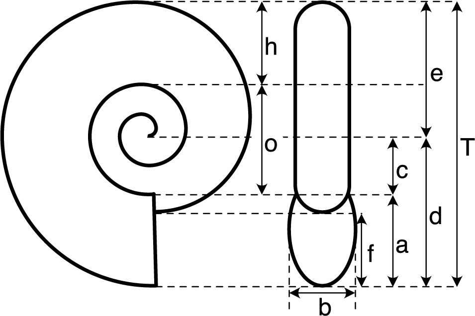
Morphometric analysis was conducted using a database containing a high-quality image for each species. The image had to depict a presumed adult shell, either as a photograph or a high-quality drawing, taken from both the side and front views. The image also needed to be sufficiently sharp and well preserved, ensuring accurate measurement of the relevant shell elements (Fig. 2). Out of 136 species, 124 met these criteria and were measured. These measurements were used to calculate seven shape ratios (see Fig. 2), including the three classical coiling parameters defined by Raup (Reference Raup1967), which allow for a quantitative assessment of shell shape (see Ritterbush and Bottjer Reference Ritterbush and Bottjer2012; Neige et al. Reference Neige, Dera and Dommergues2013), and the three used by Ritterbush and Bottjer (Reference Ritterbush and Bottjer2012) to calculate Westermann morphospace, which to some extent allows inference of hypothetical modes of life based on shell shape. Referring to the measurements described in Figure 2, the ratio calculations are as follows: D = c/d, S = b/a, W = (d/e)2, AH = f/a, U = o/T, RW = b/T, and WE = a/h.
Morphometric measurements of ammonite shells. The seven shape ratios used in this study are: D = c/d, S = b/a, W = (d/e)2, AH = f/a, U = o/T, RW = b/T, and WE = a/h (see Raup Reference Raup1967; Ritterbush and Bottjer Reference Ritterbush and Bottjer2012; Neige et al. Reference Neige, Dera and Dommergues2013).

Morphological disparity represents shape diversity and can be visualized either by the distribution of individuals within a morphological space or by numerical values characterizing this space (Roy and Foote Reference Roy and Foote1997). Note that because morphological disparity is quantified here using only the general shell shape, and not the detailed features or ornamentation used for species delimitation, we consider that morphological disparity and taxonomic diversity are not a priori correlated (see Neige [Reference Neige2003] or Roy and Foote [Reference Roy and Foote1997] for a discussion of this point). Here, morphological space was computed using PCA. The analysis incorporated the seven shape ratios derived from shell measurements (see Fig. 2). PCA was performed using a correlation matrix to ensure that all shape ratios contributed equally to the calculation. This method maximizes variation along the first axis, with each successive orthogonal axis capturing progressively less variance. Using a PCA-based approach avoids calculating disparity parameters directly within Raup’s morphospace—a method shown to be problematic (Gerber Reference Gerber2017), as Raup’s morphospace lacks a Euclidean structure. As a result, identical distances between pairs of points in Raup’s morphospace may correspond to different levels of shape dissimilarity. However, in our case, dactylioceratids exhibit highly similar shell shapes and are therefore tightly clustered within Raup’s morphospace (see “Results”), which minimizes the impact of this non-Euclidean issue. Moreover, applying PCA allows the inclusion of additional shape variables that enrich shell quantification (see Ritterbush and Bottjer Reference Ritterbush and Bottjer2012).
For disparity-based analyses, each component axis was rescaled by the square root of its eigenvalue, so that each axis contributed proportionally to the total variation (PC 1 more than PC 2, and so on). Because the number of retained components was less critical in this approach, all components were included in the calculation of the mean pairwise distance (MPD)—the mean Euclidean distance between each pair of points in the dataset. MPD is robust to sample size variations (Foote Reference Foote1992) and is minimally affected by sampling coverage (Ciampaglio et al. Reference Ciampaglio, Kemp and McShea2001). This analysis was performed at the subchronozone scale, except for the Apyrenum subchronozone, where insufficient data prevented reliable calculations (of the two species in this subchronozone, only one could be measured). In each case, results were bootstrapped 1000 times to obtain a 95% confidence interval. The use of different disparity parameters is recommended to thoroughly explore morphological disparity across different evolutionary contexts (Ciampaglio et al. Reference Ciampaglio, Kemp and McShea2001). This recommendation is particularly pertinent when studying extinction patterns (Korn et al. Reference Korn, Hopkins and Walton2013; Dai et al. Reference Dai, Korn and Song2021). Therefore, to further investigate morphological disparity, three additional parameters were computed: sum of variance (SumVar), area of convex hull (ACH), and sum of ranges (SumRanges). For these three additional parameters, results were bootstrapped 1000 times to obtain a 95% confidence interval and rarefied to n = 8, as these disparity metrics are sensitive to sample size. Beyond the recommendation to use multiple, and ideally complementary, disparity metrics, broader considerations on how to construct and interpret morphospaces—whether in an extinction context or not—are extensively discussed in the literature (e.g., Roy and Foote Reference Roy and Foote1997; McGhee Reference McGhee1999; Hopkins and Gerber Reference Hopkins, Gerber, de la Rosa and Müller2017; Polly Reference Polly2023). Altogether, careful attention should be paid to the methods used to compute both morphospaces and disparity parameters, always bearing in mind that these are only proxies for biological reality. This warrants caution when interpreting results, especially when working with fossil species.
Results
Species Richness through Time and Space
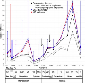
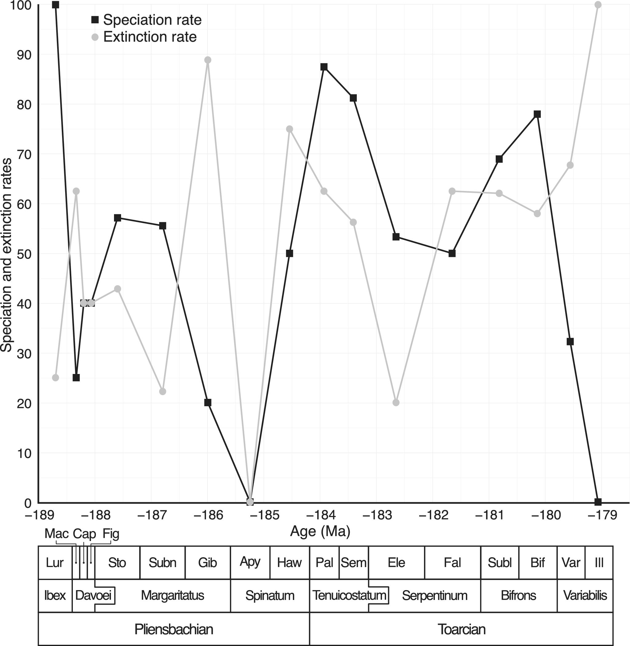
A total of 136 species of Dactylioceratidae were recorded from the Luridum to Illustris subchronozones (Fig. 3). Among these, 70 species (51.5%) were found in only one subchronozone (temporal singletons) and 56 species (41.2%) were endemic to a single domain (geographic singletons). The overall sampling coverage for Dactylioceratidae was estimated at 83.1% (ICE method). Coverage values for individual subchronozones were generally above 0.7, except for Apyrenum, which had a very low (0.2) coverage (Supplementary Fig. S1), indicating poor fossil record quality for that time bin. The various species richness curves obtained (raw data, excluding temporal and paleogeographic singletons, ICE, and Chao2) display a similar pattern (Fig. 3), with the number of temporal singletons generally lower than that of geographic singletons. The global species richness trend shows an initial increase during the Pliensbachian (Gibbosus subchronozone), followed by a sharp decline just before the end of the stage, preceding the T-OAE extinction event. The Toarcian is characterized by a gradual increase in species richness, peaking during the Bifrons subchronozone, before undergoing a steep decline leading to the final extinction of Dactylioceratidae in the Illustris subchronozone. The ICE and Chao2 diversity estimators suggest the presence of a few additional species during the Capricornus and Figulinum subchronozones, as well as at the beginning of the Toarcian. Speciation and extinction rates are highly variable (Fig. 4), and a surprising 0% extinction and speciation rate is observed during the Apyrenum subchronozone. This anomaly is clearly due to the poor fossil record for this interval, as previously noted. At the end of the clade’s history, following a peak during the Bifrons subchronozone, the speciation rate drops drastically twice (Variabilis then Illustris subchronozones), reaching zero in the last subchronozone. Meanwhile, the extinction rate is slightly delayed, showing a significant increase only during the final subchronozone.
Dactylioceratidae raw species richness (thick black line with square symbols), without temporal singletons (light gray line with triangle symbols), without geographic singletons (medium gray line with diamond symbols), compared with the corresponding estimators Chao 2 (blue line with circle symbols) and incidence‐based coverage estimator (ICE; red line with square symbols). Chao2 and ICE estimators include 95% confidence intervals computed by bootstrap resampling. Data are plotted at the midpoints of the time scale of Gradstein et al. (Reference Gradstein, Ogg, Schmitz and Ogg2020). The lower part of the figure shows the chronostratigraphic framework used here at the stage, chronozone, and subchronozone scales. Lur, Luridum sz; Mac, Maculatum sz; Cap, Capricornus sz; Fig, Figulinum sz; Sto, Stokesi sz; Subn, Subnodosus sz; Gib, Gibbosus sz; Apy, Apyrenum sz; Haw, Hawskerense sz; Pal, Paltus sz; Sem, Semicelatum sz; Ele, Elegantulum sz; Fal, Falciferum sz; Subl, Sublevisoni sz; Bif, Bifrons sz; Var, Variabilis sz; Ill, Illustris sz. Black arrows indicate the two pulses of the second-order Toarcian crisis.

Speciation (black square symbols) and extinction (gray circle symbols) rates for Dactylioceratidae. Note that the 0% extinction and speciation rate for Apyrenum subchronozone is due to a dramatically poor fossil record (see Supplementary Fig. S5).

With the exception of the Apyrenum subchronozone, the Southern Tethys and Northwest Tethys are the two domains where most species are found (Fig. 5), whereas Australasia and Southeast Asia exhibit very low diversity. In general, temporal singletons are rare during the Pliensbachian, and approximately half of the species are endemic (Fig. 3). Initially, Dactylioceratidae are predominantly found in the Southern Tethys, but they also occur in the Northwest Tethys, Arctic, and Northwest America. The occupation of domains and spatial units varies over time (Fig. 5). At the beginning of the clade’s history, 50% of domains are occupied. However, geographic occupation declines sharply from the late Pliensbachian onward before recovering, reaching its peak during the Bifrons subchronozone, when Dactylioceratidae species are present in 100% of domains and 86% of spatial units. Following this peak, occupancy declines again to around 50% for both domains and spatial units. Dactylioceratidae disappear first from Southeast Asia and Australasia. In the Illustris subchronozone, they vanish first from Northwest America, followed by the rest of the world, marking their final extinction.
Percentage of geographic occupation of Dactylioceratidae for spatial units (gray line) and domains (black line). The stacked graph expresses number of species within any of the eight domains over time (colors are the same as in Fig. 1). In this graph, a single species may be counted several times if it occurs in multiple domains within a given subchronozone.

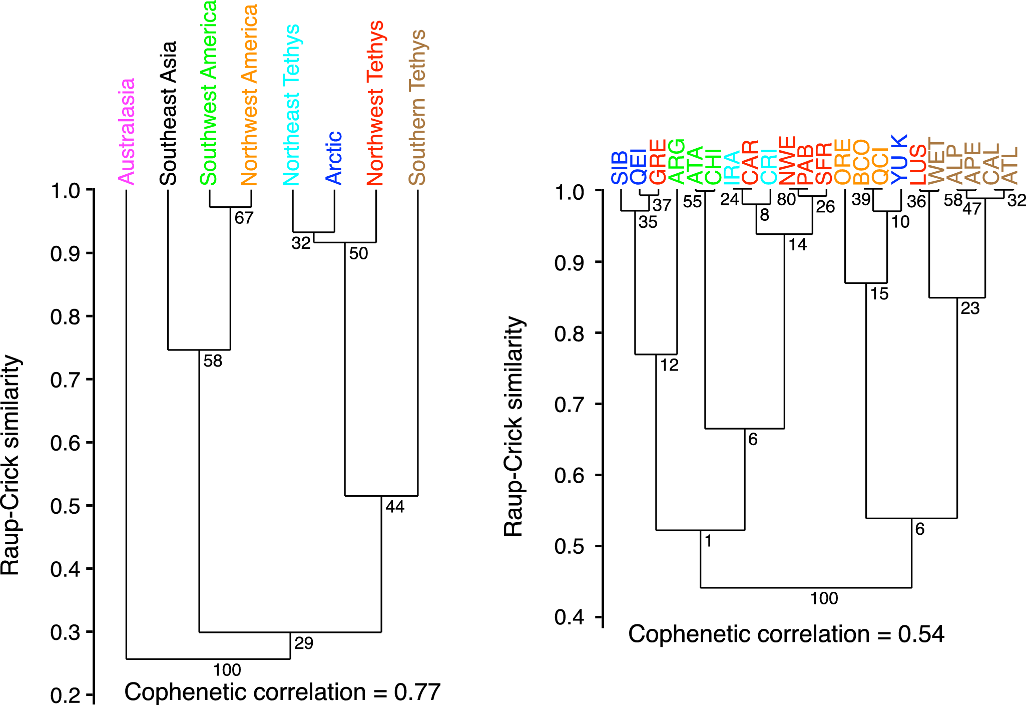
The clustering of domains (Fig. 6) for the entire database, without considering time, reveals two main faunal clusters, with Australasia forming a distinct outgroup. The first cluster consists of the Pacific domains, where Northwest and Southwest America share the most similar faunas. The second cluster is Tethyan, which also includes the Arctic. Within this group, Southern Tethys is the most distinct from the others. The Pacific cluster nodes are the only ones with a robustness greater than 50%. Clustering at the spatial unit scale reveals a slightly less distinct structure, particularly for Southwest America: the Argentine fauna shows Arctic affinities, the Atacama and North Chile units are closer to Northern Tethys. Three Northwest Tethys units stand out: the Carpathian Mountains cluster with Northeast Tethys, Greenland shares faunal similarities with the Arctic, and the Lusitanian Basin has a strong affinity with Southern Tethys. The Southern Tethys units again appear quite distinct from the rest of the Tethyan domains, while the Yukon spatial unit clusters with Northwest America. With a cophenetic correlation coefficient of 0.55, this clustering poorly represents similarities between spatial units, and most cluster nodes lack robustness. Clustering at the subchronozone level was also performed, but it is not included in this paper, as it did not reveal any significant patterns.
Similarity analysis of Dactylioceratidae assemblages within the eight geographic domains, represented by cluster dendrograms for the complete database. Node values given by bootstrap resampling. Preservation of pairwise distances between original data points measured by the cophenetic correlation coefficient.

Morphological Disparity of Dactylioceratidae and through Time
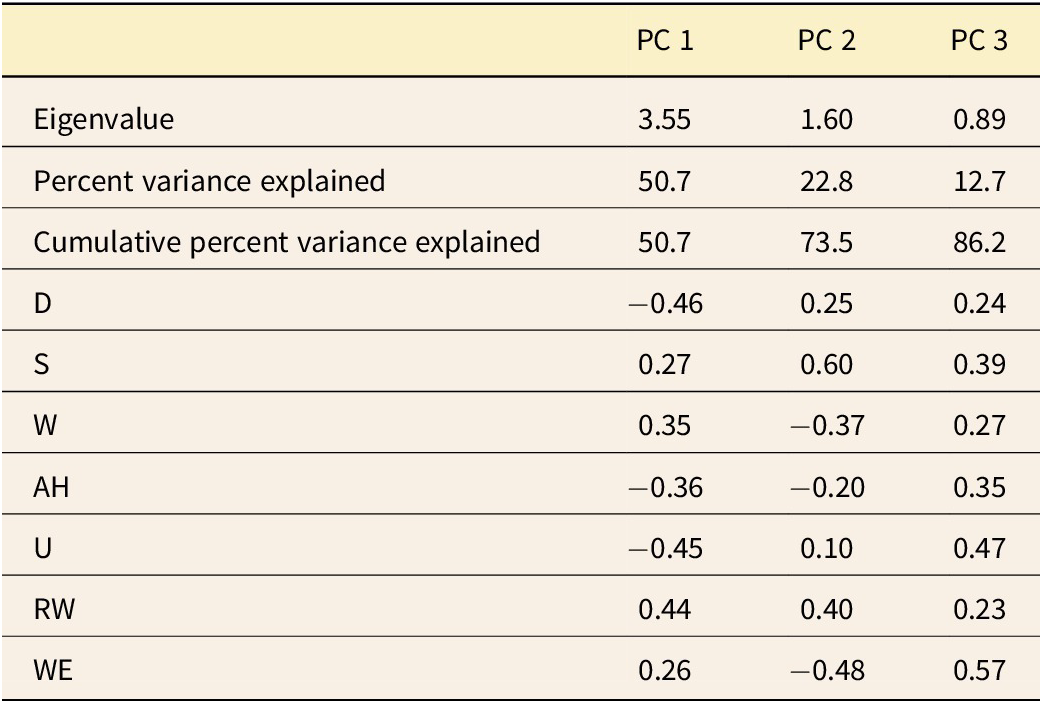
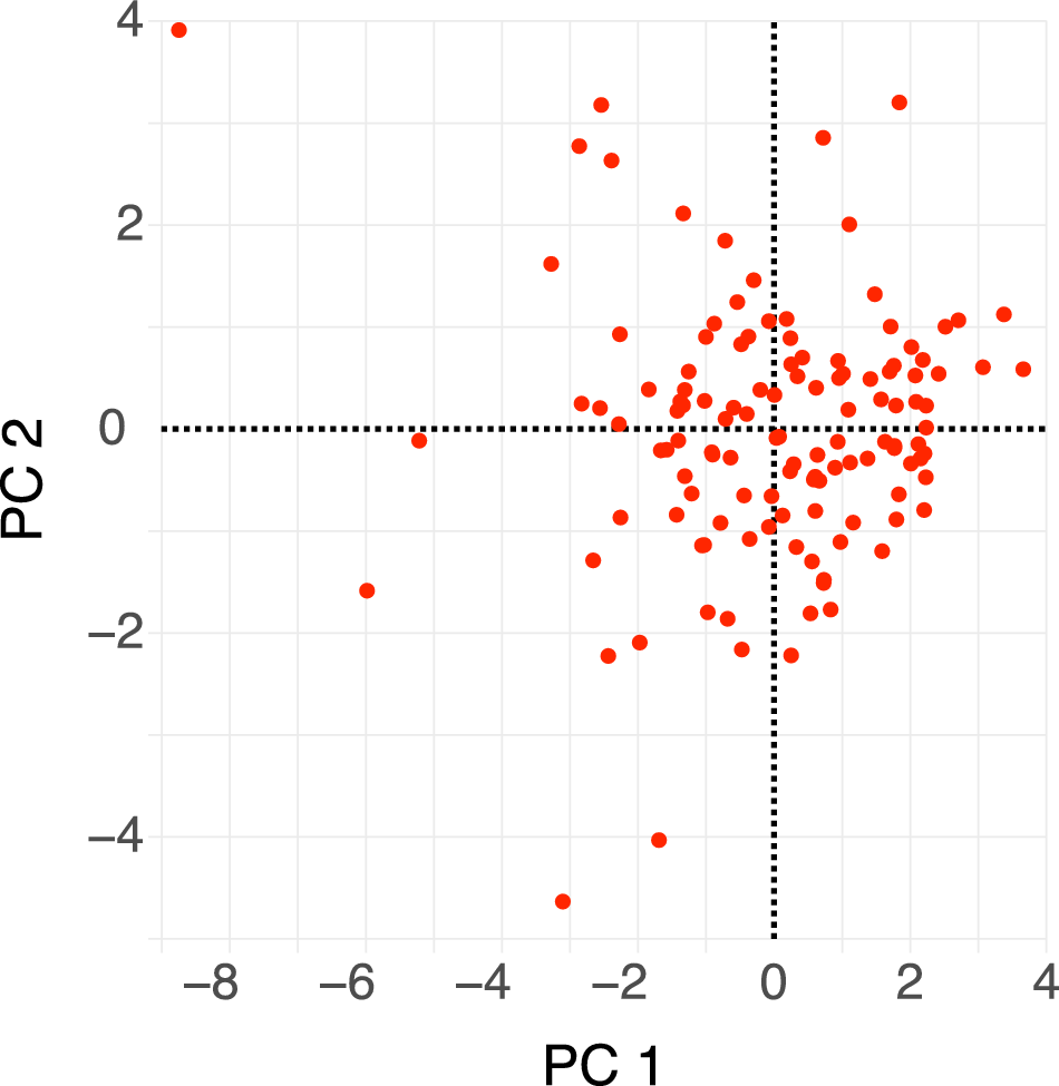
Dactylioceratidae as a whole exhibit a narrow range of shell shapes compared with the full spectrum of shell shapes seen in ammonoids (Fig. 7). They are primarily concentrated in serpenticone shapes (high D values and low W values), while rare shells exhibit cadicone shapes (medium D and W values). This confirms (and was largely observable in the shells themselves) the typical and “conservative” shape of Dactylioceratidae shells (see also Neige et al. Reference Neige, Dera and Dommergues2013: fig. 7). Following Westermann’s hypothesis, their shapes mostly reflect a planktonic mode of life (Fig. 7, bottom). Other morphotypes occupy the demersal zone or even the vertical migrant and nekton zones, which may indicate greater ecological specialization. PCA reveals that the first two PCs explain 73.5% of the variance (Table 1). PC 1 (Fig. 8) is influenced by coiling type and shell thickness: positive values correspond to the most evolute and compressed shells, while negative values correspond to the most involute and depressed shells. PC 2 divides Dactylioceratidae into forms with a large shell expansion rate and a compressed section (negative values) and those with slower shell growth and a more depressed section (positive values). In this first factorial plane, most points are clustered, while they are more scattered along PC 2 than on PC 1. For PC 3, all the variables are correlated with each other, and the points are scattered along this axis. This PC separates slightly involute shells with a low (negative) growth rate from fully involute shells with a higher (positive) growth rate.
Position of Dactylioceratidae shells (red circles) within Raup shape-space (D vs. W) and within Westermann morphospace. Top, comparison with hypothetical shell forms (redrawn from Raup Reference Raup1967: text-fig. 3). Middle, comparisons with contoured density of natural occurrence of planispiral ammonoids (redrawn from Raup Reference Raup1967: text-fig. 4). Bottom, position within Westermann morphospace (redrawn, simplified, and modified from Ritterbush and Bottjer Reference Ritterbush and Bottjer2012) following the Ritterbush and Bottjer (Reference Ritterbush and Bottjer2012) method. This ternary morphospace infers the general mode of life of ammonoids from shell shape, following Westermann’s (Reference Westermann, Tanabe and Davis1996) hypothesis. Some specimens may plot outside Westermann morphospace due to extreme shapes that were not included in the database initially used by Ritterbush and Bottjer (Reference Ritterbush and Bottjer2012) when defining the morphospace.

Results from the principal component analysis (PCA) of seven morphological indices of the Dactylioceratidae dataset: eigenvalues, percent variance explained, cumulative percent variance explained, and relative weights of variables.

Morphospace of Dactylioceratidae shells (PC 1 vs. PC 2). This first factorial plane represents 73.5% of total variance (50.7% and 22.8% along PC 1 and PC 2, respectively).

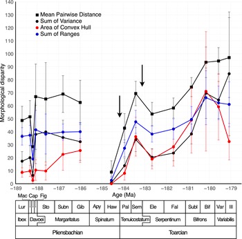
Results for the four disparity parameters (MPD, SumVar, ACH, and SumRanges) are quite similar, except at the end of the clade’s history (Fig. 9). Disparity fluctuates at the very beginning of the studied period, then remains relatively stable up to the Gibbosus subchronozone. However, ACH shows an increase at that time. At the very end of the Pliensbachian, disparity is very low (partly due to the very low number of species) and increases through the beginning of the Toarcian, with a peak during the Semicelatum subchronozone. Interestingly, the first pulse of the T-OAE extinction (at the beginning of the Toarcian) is not recorded for Dactylioceratidae (see Fig. 9, left arrow), whereas the second one (after the Semicelatum subchronozone) is slightly pronounced (see Fig. 9, right arrow). After that decrease, morphological disparity (this is true for the four parameters shown here) follows a continuous increase until the Bifrons subchronozone, where it reaches high values. Focusing on the end of the clade’s period of existence reveals contrasting disparity patterns. First, morphospace occupation increases between the Sublevisoni and Bifrons subchronozones (Fig. 10). Then, some extreme shapes disappear during the Variabilis subchronozone (Fig. 10). The last subchronozone before complete extinction (Illustris) is marked by an even more pronounced disappearance of some shell shapes: only shapes from the lower part of the morphospace remain. This concretely indicates the disappearance of the most involute and depressed shells. This pattern is revealed by the ACH disparity parameter (which is sensitive to the presence or absence of extreme shapes in the morphospace) (Fig. 9), which drastically decreases during the last two subchronozones. It is also indicated (even if the pattern is less marked) by SumRanges. In contrast, MPD and SumVar show stability (MPD) or increase (SumVar) up to the end of the clade’s existence. These patterns suggest that the final extinction is first visible in certain shell shape types (decline of ACH and SumRanges values) before the extermination of all shapes, while the disparity of the remaining shapes in the morphospace remains largely unchanged compared with the pre-extinction phase (SumVar and MPD do not decrease). This is likely due to a reorganization of the distribution of points in the morphospace at the very end of dactylioceratid history (Illustris subchronozone). Without any increase in overall morphospace occupation, disparity rises, because the distances between points (i.e., species) become greater, as intermediate forms have been eliminated (see Fig. 9, mean pairwise distance and sum of variance, and Fig. 10, bottom right diagram).
Global disparity of Dactylioceratidae: mean pairwise distance (black squares), sum of variance (black circles), area of convex hull (red circles), and sum of ranges (blue circles). Note that mean pairwise distance values have been multiplied by a factor of 10 and sums of ranges by a factor of 2 for graphical reasons. Error bars indicate 95% confidence intervals obtained from 1000 bootstrap replicates. No disparity value for Apyrenum subchronozone, because only one species is available for measurements (see text). Black arrows indicate the two pulses of the second-order Toarcian crisis.

Morphospace of Dactylioceratidae shells (PC 1 vs. PC 2) for the last four subchronozones before the clade’s extinction: Sublevisoni, Bifrons, Variabilis, and Illustris from oldest to latest, respectively. Red dots for shapes found in a given subchronozone. Gray dots indicate the overall morphospace.

Discussion
Dactylioceratidae Compared with Ammonoids
The present study aligns well with previous studies on ammonites from the same time period (Macchioni and Cecca Reference Macchioni and Cecca2002; Cecca and Macchioni Reference Cecca and Macchioni2004; Dera et al. Reference Dera, Neige, Dommergues, Fara, Laffont and Pellenard2010; Caruthers et al. Reference Caruthers, Smith and Gröcke2013; Neige et al. Reference Neige, Dera and Dommergues2013). However, it should be noted that these comparisons must be made with caution because: (1) previous studies focus on ammonoids as a whole, so some Dactylioceratidae species are included in their datasets, making them not entirely independent from the present one; and (2) comparisons with these previous studies may be challenging due to differences in temporal resolution (subchronozones here vs. chronozones in the previous studies).
During the lifetime of Dactylioceratidae, previous studies on all ammonoids highlighted four extinction events: during the Gibbosus subchronozone, at the Pliensbachian/Toarcian transition, during the Semicelatum subchronozone, and at the Bifrons/Variabilis transition. The Pliensbachian/Toarcian and Bifrons/Variabilis transition events have also been identified at the generic level for ammonites in Argentina (Riccardi Reference Riccardi2008). Of these, only two are clearly visible in Dactylioceratidae: the Gibbosus and Bifrons/Variabilis transitions (Fig. 3). Both events are associated with a drop in sea temperatures, along with the onset of a regression phase for the Bifrons/Variabilis transition (Dera et al. Reference Dera, Brigaud, Monna, Laffont, Pucéat, Deconinck, Pellenard, Joachimski and Durlet2011a; Haq Reference Haq2017). The Pliensbachian/Toarcian event is marked by an increase in the specific diversity of Dactylioceratidae in contrast to ammonoids as a whole. This pattern may also occur in ammonoids overall but is restricted to a particular paleogeographic area: the Northwest Tethys (Cecca and Macchioni Reference Cecca and Macchioni2004). The decrease in diversity at the start of the Davoei chronozone (i.e., the Maculatum subchronozone) is also observed in other ammonoid groups, but it has not been considered an extinction event. It seems to mainly result from a decrease in speciation, according to Dera et al. (Reference Dera, Neige, Dommergues, Fara, Laffont and Pellenard2010).
There is a shift in speciation rates between ammonoids in general and Dactylioceratidae at the Pliensbachian/Toarcian transition. In ammonoids, speciation increases during the upper Pliensbachian, supporting the Gibbosus event (Dera et al. Reference Dera, Neige, Dommergues, Fara, Laffont and Pellenard2010; Caruthers et al. Reference Caruthers, Smith and Gröcke2013). Speciation then drops at the transition between the Pliensbachian and the Toarcian, followed by a slight rise (Dera et al. Reference Dera, Neige, Dommergues, Fara, Laffont and Pellenard2010). For Dactylioceratidae, the speciation rate is not very high at the beginning of the upper Pliensbachian and decreases during the Gibbosus and Apyrenum subchronozones. It then increases sufficiently to almost double the number of species during the Paltus and Semicelatum subchronozones. Afterward, the extinction and speciation rates of Dactylioceratidae begin to follow the trends observed in ammonoids in general. The decline in speciation during the Bifrons–Variabilis event is also observed in ammonoids (Dera et al. Reference Dera, Neige, Dommergues, Fara, Laffont and Pellenard2010), but it is definitive in Dactylioceratidae and ultimately leads to the extinction of the clade. This decline occurs in the context of a marine regression (see “Introduction”), which led to a reduction in epicontinental environments during the Variabilis Zone (Sandoval et al. Reference Sandoval, O’Dogherty and Guex2001), which could explain the collapse of numerous ammonoid taxa associated with these environments, as well as the persistence of certain oxyconic clades such as the phylloceratids (Dera et al. Reference Dera, Neige, Dommergues, Fara, Laffont and Pellenard2010), generally considered to inhabit open and deeper marine settings (Westermann Reference Westermann, Tanabe and Davis1996). The observed decline in species rate may therefore be related to the contraction of habitats occupied by dactylioceratids: by reducing habitat, regression limits opportunities for allopatric or ecologically driven divergence, thereby constraining the emergence of new species.
Dactylioceratidae morphology is relatively homogeneous over time. At the Maculatum/Capricornus transition, disparity decreases, probably due to selective extinction against less evolute shapes. The high disparity value observed in the Figulinum subchronozone is mainly due to a species (Bettoniceras perisphinctoides) with an extreme shape (a highly evolute whorl with a compressed cross-sectional shape, which gives this species an extremely negative value on PC 2). The disparity decrease observed for ammonoids during the Gibbosus event (Dera et al. Reference Dera, Neige, Dommergues, Fara, Laffont and Pellenard2010) does not occur in Dactylioceratidae. During the Semicelatum event, there was no disappearance of particular forms in the studied clade, whereas for the period considered here, this is the only morphologically selective extinction event identified among the complete ammonoid clade (see Dera et al. Reference Dera, Neige, Dommergues, Fara, Laffont and Pellenard2010). Disparity patterns at the end of the Dactylioceratidae history clearly show selective extinction (Foote Reference Foote1991): species richness and disparity (as seen with the ACH disparity parameter) decline (Fig. 9), with shell shapes from the upper part of the morphospace disappearing (Fig. 10). However, this selective extinction is paradoxically not revealed by SumVar and MPD, which remain stable (MPD) or slightly higher (SumVar). This is due to a reorganization of the species’ positions at the end of the clade’s history: fewer species are present, but their positions remain stable, resulting in a more scattered distribution across the morphospace than before and in higher disparity levels for SumVar and MPD than expected (Foote Reference Foote1993). This pattern of selective extinction in Dactylioceratidae contradicts the patterns observed in ammonoids of the same age, as exemplified by Dera et al. (Reference Dera, Neige, Dommergues, Fara, Laffont and Pellenard2010).
Dactylioceratidae reveal paleobiogeographic patterns similar to those of ammonoids as a whole (Page Reference Page2008): the Northwest and Southwest America domains show similarities, as do the Northeast, Northwest, Southern Tethys, and Arctic domains. These similarities, observed both at the domain level and throughout the complete history of the Dactylioceratidae clade, indicate a strong biogeographic imprint and the absence of significant mixing of species throughout the clade’s history. The pattern observed at the spatial-unit scale, however, is much more blurred, and comparisons with previously published results are somewhat difficult due to the high temporal resolution used here.
Dera et al. (Reference Dera, Neige, Dommergues and Brayard2011b) studied ammonoid biogeographic distribution for the Northwest Tethyan realm (Northeast, Northwest, and Southern Tethys in the present study) and the Arctic realm (Arctic domain in the present study) during a comparable geological time. They demonstrated a faunal dichotomy (provincialism) between the Northern and Southern Tethys throughout the Pliensbachian, directly linked to paleogeographic barriers and latitudinal paleoclimatic and paleoecological contrasts. This pattern was progressively lost during the Toarcian due to a major sea-level rise, a global warming event, and the T-OAE mass extinction, which preferentially removed endemic species. This same pattern is also noticeable in Dactylioceratidae. The singular pattern of the Lusitanian Basin can be interpreted similarly: although located in the Northwest Tethys, it is generally associated with the ammonoid fauna of the Southern Tethys, because at the beginning of the Toarcian, this basin saw the arrival of a south Tethyan fauna (Dera et al. Reference Dera, Neige, Dommergues and Brayard2011b; Rocha et al. Reference Rocha, Mattioli, Duarte, Pittet, Elmi, Mouterde and Cabral2016). This holds true for Dactylioceratidae as well (Fig. 6, right). Only a few details differ when comparing the paleobiogeographic patterns of Dactylioceratidae and other ammonoid groups. For example, the similarity between the Arctic ammonoid fauna and that of the Northwest Tethys, as revealed by Page (Reference Page2008), is not observed in Dactylioceratidae (Fig. 6).
Dactylioceratidae Extinction Due to Increased Specialization?
As mentioned earlier, the evolutionary dynamics of Dactylioceratidae may serve as a model to illustrate the hypothesis that clade extinction in the context of background extinction may be driven by species specialization (see Raia et al. Reference Raia, Carotenuto, Mondanaro, Castiglione, Passaro, Saggese and Melchionna2016). At the beginning of a clade’s existence, its species richness and geographic range increase simultaneously, while its extinction rate remains relatively low. As species specialize in ecological niches, there is a greater likelihood that they will coexist without competing with each other. However, this specialization can act as an evolutionary trap, because specialized species are more vulnerable to extinction than generalists (Vrba Reference Vrba1987; Colles et al. Reference Colles, Liow and Prinzing2009; Raia et al. Reference Raia, Carotenuto, Mondanaro, Castiglione, Passaro, Saggese and Melchionna2016). Specialization can therefore become a factor contributing to the decline or even extinction of a clade: it leads to the isolation of populations, which may promote extinction (Vrba Reference Vrba1987). According to this model, for a given clade, there must be an increase in sympatry and diversity preceding its extinction. Once peak sympatry is reached, both speciation declines and/or extinction rates increase (Raia et al. Reference Raia, Carotenuto, Mondanaro, Castiglione, Passaro, Saggese and Melchionna2016). Alongside the rise in sympatry, speciation and extinction rates should also be higher for a clade containing specialist species.
The history of the clade under study here shows an initial phase of relatively low species numbers and a small number of occupied spatial units (Figs. 3, 5), followed by a drastic increase in geographic occupation, which largely precedes the rise in species richness: at the end of the Pliensbachian for the former (Fig. 5) and in the middle of the Toarcian for the latter (Fig. 3), with a time lag of about 4 Myr. This suggests that the first part of Dactylioceratidae history is characterized by a relatively low number of species occupying few spatial units, then a still low number of species occupying many spatial units, and finally, a large number of species occupying the same number of spatial units. This suggests a potential rise in sympatry (although further investigations are needed to confirm this), a pattern that seems to fit Raia et al.’s (Reference Raia, Carotenuto, Mondanaro, Castiglione, Passaro, Saggese and Melchionna2016) model. In parallel, the disparity pattern closely mirrors that of species richness, except during the T-OAE extinction event, where disparity clearly drops but species richness does not. This is likely linked to the extinction event that affects other ammonoids and not Dactylioceratidae. However, outside this event, morphological disparity rises when species richness also rises. This can be interpreted as specialization: species become more distinct (disparity increases) as sympatry increases. At the end of this clade’s history, a selective extinction occurs just before complete extinction. Interestingly, the extinction of the clade is marked by a progressive reduction in its area of occurrence (Fig. 5): from a worldwide distribution during the Sublevisoni and Bifrons subchronozones, it first disappears from Australasia and Southeast Asia (Variabilis subchronozone), then from Northwest America. It is true that the ammonoid fossil record is relatively poor for Australasia and Southeast Asia (so the disappearance during the Variabilis subchronozone could be biased), but this is not the case for Northwest America, which likely represents a real geographic disappearance. Results for extinction and speciation rates are less clear (Fig. 4), but we note that extinction rates are high near the end of a clade’s history, which is expected for specialist species, accompanied by a more pronounced decline in the speciation rate. This may indicate that species have become too specialized to adapt to new environmental conditions.
Conclusion
This study, by focusing on a clade (Mollusca: Ammonoidea: Dactylioceratidae) at high taxonomic (species-level) and temporal (subchronozone) scales, offers new data on clade extinction outside mass or second-order extinction events. This clade, especially toward the end of its history (during the Toarcian), displays a pattern that fits rather well with background extinction, which could be due to species specialization (as noted, this point requires further investigation to be confirmed for dactylioceratids), including a rise in sympatry, high turnover, and then a decline in speciation, together with selective extinction followed by the complete extinction of the clade. It is important to note that, in addition to the hypothesis that species-level specialization increases extinction risk, several other mechanisms may account for clade-level extinction over evolutionary timescales (excluding mass extinctions, as the focus here is on background extinction). Some clades may experience a decline in evolutionary innovation, reducing their ability to explore new ecological or morphological spaces and ultimately making them more vulnerable to environmental change or competitive displacement (Van Valen Reference Van Valen1973; Quental and Marshall Reference Quental and Marshall2013). Competitive exclusion by ecologically similar but more efficient groups may also lead to clade replacement, as documented in various fossil successions—particularly when associated with geographic invasions by competing taxa (Sepkoski Reference Sepkoski1984; Navarro et al. Reference Navarro, Neige and Marchand2005; Jablonski Reference Jablonski2008). Finally, clade extinction may also result from stochastic processes, especially in groups with low diversity or small population sizes, where random demographic or evolutionary events can lead to extinction independently of ecological performance (Raup Reference Raup1981; Smith and Almeida Reference Smith and Almeida2020).
However, testing such a model—or more generally, testing any evolutionary model—with an extinct clade, even if it does not prevent comparisons with extant clades, is more complicated. First, the geographic extent of species cannot be calculated with equal precision due to fossil record constraints: among other reasons, fossils are only discovered when outcrops are available. However, it can be roughly approximated by the number of spatial units occupied.
Second is the characterization of species specialization, which remains to be specified. Colles et al. (Reference Colles, Liow and Prinzing2009) propose numerous criteria for linking species’ extinction to their specialization (e.g., ecological niche measured for several parameters, specialization measured at the specific level; for a more exhaustive list, refer to Colles et al. Reference Colles, Liow and Prinzing2009: table 1), but it must be admitted that most of these are difficult to achieve for fossil species. However, exploration of morphospaces together with quantifying morphological disparity parameters offers valuable tools for such specialization characterization, as was done here. Finally, an upgrade of the present study could be achieved through spatial standardization (Antell et al. Reference Antell, Benson and Saupe2024). A pragmatic standardization was used here by working at the domains level rather than at the spatial units level, thus avoiding some of the biases caused by the heterogeneous spatial distribution of fossils (by collapsing spatial unit data into larger domain data). One of our results does not seem to align with the hypothesis that a wide geographic range is associated with survivorship (see Payne and Finnegan Reference Payne and Finnegan2007): after a progressive reduction in its area of occurrence, immediately following a previously worldwide geographic range, Dactylioceratidae became extinct. However, a deeper exploration of biogeographic patterns based on spatial standardization would certainly add valuable insights into better understanding the extinction of Dactylioceratidae.
Acknowledgments
This study was supported by funding from the Observatoire des Sciences de l’Univers Terre Homme Environnement Temps Astronomie (SRO 2024). This article has been greatly improved by the comments of three anonymous reviewers.
Competing Interests
The authors declare no competing interests.
Data Availability Statement
Complete bibliography used to construct the database and data are available in the Supplementary Material available from the Dryad Digital Repository: https://doi.org/10.5061/dryad.s4mw6m9kb.


 Open access