


Non-technical Summary
The consequences of the speciation process are preserved in the fossil record, with ancestral lineages giving rise to descendant lineages. Reconstructing these evolutionary relationships is often a major goal of paleobiologists. A well-documented pattern in the fossil record is the presence of a small number of species and/or higher taxa that survive for a long time without going extinct. In paleobiological contexts, speciation is typically modeled as a time-dependent process. This means that the longer a species lives, the more likely it is to undergo one or multiple speciations. However, there has been little work exploring the lineage-level “fecundity” of such long-lived species. Some theories predict that we should expect to find a small number of lineages that give rise to many descendant species over the course of their long existences. Such “super-progenitors” may give rise to much of the diversity observed in real clades. Nevertheless, the extent to which we should expect to find these super-progenitors in the fossil record has not been well explored, and the methods commonly used to reconstruct evolutionary relationships often do not accommodate super-progenitors. Here, I explore a model of lineage diversification and fossil preservation to better understand how often paleobiologists might expect to encounter super-progenitors in the fossil record, especially after accounting for the incompleteness of fossil preservation. I find that super-progenitors should be exceptionally common in the fossil records of many clades. This highlights that phylogenetic methods and diversification approaches would benefit from incorporating them more explicitly.
Introduction
Inferring ancestor–descendant relationships among lineages has long been a focus of paleontological research. Linking sequences of temporally successive populations and lineages based on morphological similarity, a method that eventually came to be known as “stratophenetics” (Gingerich Reference Gingerich, Cracraft and Eldredge1979), enjoyed a long reign throughout the first half of the twentieth century as the dominant means to reconstruct phylogeny. Throughout this time, it was common to reconstruct long-lived and widespread ancestors as giving rise to multiple descendant lineages. I will refer to such taxa hereafter as “super-progenitors” following Gottlieb (Reference Gottlieb2004) and Caetano and Quental (Reference Caetano and Quental2023). These reconstructions anticipated later developments in evolutionary and ecological theory that predicted that single lineages robust to extinction may give rise to many descendant lineages (Raup et al. Reference Raup, Gould, Schopf and Simberloff1973; Hubbell Reference Hubbell2001, Reference Hubbell2005). These theoretical predictions have turned out to be consistent with empirical results in both fossil (Wagner and Erwin Reference Wagner, Erwin and Anstey1995) and living (Schluter and McPhail Reference Schluter and McPhail1992) organisms.
The conception of super-progenitor lineages developed here builds upon a particular mode of species origination now often referred to as “budding” cladogenesis, in which an ancestor gives rise to a descendent lineage and continues to coexist alongside the new species. A budding-like pattern was depicted by Rensch (Reference Rensch1959), who also discussed its macroevolutionary implications. The term “budding” emerged gradually throughout the years, used mostly by neontological workers (e.g., Grant and Grant Reference Grant and Grant1967; Wiley Reference Wiley1978; Wiley and Mayden Reference Wiley and Mayden1985; Glazier Reference Glazier1987), who would usually draw an explicit link to Mayr’s concept of speciation by peripheral isolation, a form of allopatry in which a small subpopulation becomes isolated at the edge of a species range and undergoes rapid divergence (Mayr Reference Mayr1963, Reference Mayr1982). This pattern also gained popularity in explaining patterns in the fossil record (Eldredge and Gould Reference Eldredge, Gould and Schopf1972). All along, paleobiologists had been depicting speciation in a similar way, based upon their observations of the temporal distribution of closely related species. This was reflected in early modeling approaches, which all assumed a budding mode of species generation (Raup et al. Reference Raup, Gould, Schopf and Simberloff1973; Raup and Gould Reference Raup and Gould1974; Raup Reference Raup1985) without referring to it as such. A set of speciation “modes” were eventually operationalized by paleobiologists, and the term “budding” was adopted to describe the common scenario depicted throughout this thread of earlier work (Archibald Reference Archibald1993; Wagner and Erwin Reference Wagner, Erwin and Anstey1995; Foote Reference Foote1996).
Budding differs from “splitting” or “bifurcating” cladogenesis, in which a single ancestral lineage divides its population roughly equally, giving rise to exactly two descendants simultaneously while going extinct (or rather, “pseudo-extinct”) itself. Bifurcation has typically been the preferred mode of many workers due to its natural link to cladograms and vicariance biogeography (Hennig Reference Hennig1966; Brooks and McLennan Reference Brooks and McLennan1991). Despite this appeal, bifurcation appears to be relatively rare from an empirical standpoint (Wagner and Erwin Reference Wagner, Erwin and Anstey1995). On the other hand, budding appears to be common among fossil lineages and is often favored by paleobiologists. One major appeal of budding also lies in its link to the neontological theories of geographic speciation propagated by Mayr and modified by others. The general formula of allopatry in a small subpopulation has largely survived scrutiny among population geneticists, including those who disagree with several of Mayr’s other views on speciation (Coyne Reference Coyne1994). More recent work in living organisms has shown that the peripheral isolation model appears fairly common (Toussaint et al. Reference Toussaint, Sagata, Surbakti, Hendrich and Balke2013; Anacker and Strauss Reference Anacker and Strauss2014; Kruckenhauser et al. Reference Kruckenhauser, Duda, Bartel, Sattmann, Harl, Kirchner and Haring2014; Kaya and Çiplak Reference Kaya and Çiplak2016; Ivey et al. Reference Ivey, Habecker, Bergmann, Ewald, Frayer and Coughlan2023), although not universal (e.g., Blair et al. Reference Blair, Heckman, Russell and Yoder2014), providing an additional neontological clue for the importance of budding speciation and the strong potential for the commonness of super-progenitor lineages in the fossil record.
Despite the strong empirical evidence for budding and its theoretical appeal, the topic of super-progenitors has been relatively under-explored due to methodological limitations. For decades, it was common and uncontroversial to depict complex arrangements between ancestors and descendants. This protracted period of methodological stability came to a quick end with the emergence of cladistic methodologies for phylogenetic reconstruction in the 1970s. Cladists were adamant that ancestor–descendant relationships were untestable and sought to bring greater rigor to phylogenetic analysis by replacing the largely qualitative methodologies long employed by paleontologists with a set of quantitative and algorithmic approaches to the reconstruction of bifurcating trees depicting only nested patterns of inheritance of novel character states (i.e., cladograms), while omitting any explicit phylogenetic statements, such as ancestor–descendant relationships (Platnick Reference Platnick1977; Nelson and Platnick Reference Nelson and Platnick1981).
The methodological and philosophical revolution brought forth by cladistics introduced unprecedented rigor to paleobiology but also left deep scars. The phylogenetic methods available to paleobiologists over the past several decades have inherited limitations imposed during the bygone cladistic era. While important developments have greatly improved paleobiologists’ ability to evaluate ancestor–descendant relationships (Fisher Reference Fisher, Grande and Rieppel1994; Wagner Reference Wagner1998; Stadler Reference Stadler2010; Stadler et al. Reference Stadler, Gavryushkina, Warnock, Drummond and Heath2018), most existing tree reconstruction methods do not test arrangements where more than two descendants stem from a single ancestor (Marcot and Fox Reference Marcot and Fox2008; Gavryushkina et al. Reference Gavryushkina, Welch, Stadler and Drummond2014; Höhna et al. Reference Höhna, Landis, Heath, Boussau, Lartillot, Moore, Huelsenbeck and Ronquist2016; Parins-Fukuchi Reference Parins-Fukuchi2021). This limits paleobiologists’ ability to reconstruct phylogeny. Nevertheless, some existing modeling approaches offer a natural path to incorporating such patterns by representing the full stratigraphic ranges of taxa (Stadler et al. Reference Stadler, Gavryushkina, Warnock, Drummond and Heath2018). More recently, a newly developed phylogenetic method has harnessed these models to explicitly test for super-progenitors (Stolz et al. Reference Stolz, Gavryushkina, Vaughan, Stadler and Allen2025). Although the general notion that certain long-lived lineages may give rise to many descendants has long been recognized in paleobiology (Raup et al. Reference Raup, Gould, Schopf and Simberloff1973; Wagner and Erwin Reference Wagner, Erwin and Anstey1995; Wagner Reference Wagner2019; Wright and Wagner Reference Wright and Wagner2024), the expected variation in the number of descendants is rarely explored. Given the increasing availability of models and tools that accommodate super-progenitors, an exploration of the frequency at which we might expect to encounter them and the conditions that tend to give rise to them would be a timely contribution.
A large presence of super-progenitors in phylogenetic datasets would carry many important implications. Understanding their prevalence might shed light on the macroevolutionary and macroecological processes that mediate the origin and maintenance of biodiversity preserved in the fossil record. The stochastic birth–death processes frequently used in paleobiological studies predict that super-progenitors should be common (e.g., Raup et al. Reference Raup, Gould, Schopf and Simberloff1973). More sophisticated models that account for differences in population size among species in the tree agree, but predict an even more skewed distribution of descendants, with the vast majority of speciation events stemming from a relatively small number of progenitors with intermediate and large abundances (Hubbell Reference Hubbell2001). Generating a more complete image for how descendant lineages are distributed across phylogenies may help to shed light on the mechanisms that drive the evolution of clades. Super-progenitors could also greatly impact phylogenetic reconstruction. If super-progenitors are common, methods that fail to entertain hypotheses where ancestors can give rise to multiple descendant lineages will be misled. Super-progenitor–like patterns have been occasionally proposed as an explanation for weak phylogenetic resolution (Gahn and Kammer Reference Gahn and Kammer2002). If these patterns are common, identifying them can improve our insights into the paleobiology of fossil clades.
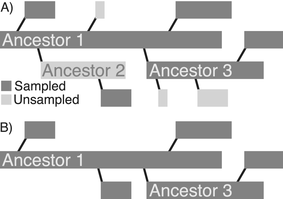
On the other hand, even though several models predict the existence of super-progenitors, it is not clear how incomplete sampling might affect their realized prevalence in fossil clades. Even if super-progenitors are common as clades evolve, it is possible that the levels of incompleteness often encountered in the fossil record frequently preclude the sampling of ancestors and a sufficient number of their descendants. In this case, even if super-progenitors themselves are common enough, the phylogenetic patterns reconstructed by paleontologists from incomplete fossil records would rarely be affected. It might therefore be useful to distinguish between super-progenitors—operationally defined here as taxa that give rise to at least two descendants—from sampled super-progenitors (hereafter referred to as SSPs) that give rise to at least two sampled descendants (Fig. 1). Additionally, because bifurcating cladogenesis also yields patterns where ancestors give rise to two descendants, it may be useful to distinguish between SSPs that give rise to at least two sampled descendants (2+ SSPs) and those that give rise to at least three sampled descendants (3+ SSPs).
A, Full radiation of a clade that includes two super-progenitors. Ancestor 1 gives rise to five total direct descendants and Ancestor 3 gives rise to three direct descendants. B, The apparent pattern of phylogenetic relationships, given incomplete stratigraphic sampling. Ancestor 1 still appears as a super-progenitor, while Ancestor 3 does not. Thus, incomplete sampling could reduce the appearance of super-progenitors in empirical datasets, even if the super-progenitors are themselves preserved in the fossil record.

Like most paleobiological diversification patterns, the proportion of SSPs will vary as a function of three parameters: origination rate (i.e., speciation rate when operating at the species level, as is the case here), extinction rate, and fossil preservation rate. One way these rates influence the distribution of SSPs is through their impact on “completeness,” or the proportion of species in the clade preserved in the fossil record and recovered by paleontologists. Completeness can be estimated as a ratio of preservation to extinction rate (Foote Reference Foote1997; Solow and Smith Reference Solow and Smith1997). Modifying the completeness of a fossil record by varying the preservation rate informs how variation in geological processes might affect the proportion of SSPs. However, this procedure does not build intuition for how variation in biological parameters (e.g., origination and extinction rate) leads to the appearance of more or fewer SSPs. While the extent to which a clade is preserved in the fossil record creates variation in the proportion of expected super-progenitors that are visible to paleobiologists, differences in evolutionary dynamics may also have a large effect. If preservation is held constant, we should expect clades experiencing higher turnover (i.e., origination plus extinction rate) to have comparatively fewer visible super-progenitors. We should also expect different dynamics to occur when origination outpaces extinction (positive net diversification) versus when extinction outpaces origination (negative net diversification).
In this study, I analyze and perform simulations using a simple birth–death-sampling (BDS) model to explore how frequently we might expect to encounter SSPs under a variety of empirically realistic parameter combinations. I also sought to examine, in turn, how the expected proportion of SSPs changes as a function of (1) variation in preservation rate and (2) differences in the process of lineage diversification. This topic could substantially influence paleobiological approaches in a variety of areas. If we can expect super-progenitors and an appreciably large number of their descendants to be preserved in the fossil record, this would have major implications for the types of lineage diversification patterns we might expect to encounter. If such patterns are common, identifying and exploring them can also open new possibilities for the exploration of evolutionary mechanisms rarely entertained in the fossil record.
Materials and Methods
BDS Model
To estimate parameters and compute probability distributions for the expected number of sampled descendants, I obtained a series of probability densities based on a simple BDS model. Very little novel analytical work was required, as I was largely able to draw upon equations derived in previous work with little to no modification. These equations draw heavily upon previous work analyzing birth–death processes (Kendall Reference Kendall1948; Raup Reference Raup1985; Foote Reference Foote1996, Reference Foote1997). Following these previous works, I modeled speciation, extinction, and fossil preservation as three independent Poisson processes. The expressions note where a term (1) was borrowed from a previous derivation, (2) reflected a standard Poisson probability density, or (3) was derived here. The particular combination of the expressions described here to compute the probability of a set of stratigraphic ranges arranged into a phylogeny is new to this study. The resulting model is similar to the “fossilized birth–death range” (FBDR) model introduced by (Stadler et al. Reference Stadler, Gavryushkina, Warnock, Drummond and Heath2018). It is simpler in that it does not explicitly accommodate for sampling fraction among extant taxa, as nearly all the clades examined here were fully extinct or had only few extant representatives and thus minimal bias. Like the simplest variant of the FBDR model, the model used here does not model bifurcating cladogenesis and instead assumes that speciation proceeds as budding.
Under the BDS framework, the expected number of sampled descendants for each lineage depends on three parameters: speciation, p; extinction, q; and sampling, r. Like the closely related model of Warnock et al. (Reference Warnock, Heath and Stadler2020), the model does not assume complete species sampling. Each species in the phylogeny is known only from its empirically observed first (of) and last (ol) preservational appearances. We will refer to the interval spanning the first and last preservational events as the observed stratigraphic range, t. The time implied by the observed stratigraphic range will virtually always be shorter than, and can never exceed, the full duration of time that the species was extant, an unknown interval we will refer to as T. In addition to the three BDS parameters, the expected number of descendants will depend on T. I compiled several equations to derive a likelihood function to optimize values for p, q, and r, which are assumed to be shared across an entire clade, and T for each taxon. Note that throughout this section, I use the term “species” to refer to sampled fossil taxa, as that is the level of operational taxonomic unit explored here, but the model could be applied unmodified to higher-level taxa as well.
The likelihood function is applied to each branch of a phylogeny individually. The likelihood for an entire clade is the joint likelihood across all branches. Separate expressions are applied to branches corresponding to fossil species (sampled ancestors) and to those with no known fossil representative (hypothetical ancestors). Once parameter estimates are found, the probability distribution for the number of observed descendants is then computed for each species in the clade.
Sampled Ancestors
For a given fossil species, the likelihood depends on three quantities under the model. Expressed verbally, these are: (1) the probability of observing a given stratigraphic duration (t) given a sampling rate (r) and lineage duration (T); (2) the probability of sampling n o observed descendant species (as reflected in the tree topology) over duration T given parameters p, q, and r; and (3) the likelihood of going extinct after duration T given extinction rate q.
The first expression, $ {L}_{\mathrm{R}} $
, is the likelihood of observing a particular stratigraphic range given sampling rate and duration and was derived for continuous time by Foote (Reference Foote1997):
$ {L}_{\mathrm{R}} $
, is the likelihood of observing a particular stratigraphic range given sampling rate and duration and was derived for continuous time by Foote (Reference Foote1997):
 $$ {L}_R={r}^2\left(T-t\right){e}^{-r\left(T-t\right)} $$
when t > 0 and
 $$ {L}_{\mathrm{R}}=P\left(t|T,r\right)=r\;T\;{e}^{- rT} $$
when t = 0 (i.e., when a lineage is known from only one time point).
The second expression, $ {L}_{\mathrm{S}} $
, gives the likelihood of n
s speciation events implied by the phylogeny and was influenced by the work of Wagner (Reference Wagner2019). Speciation is modeled as a homogeneous Poisson process and so finding the probability of an ancestral lineage giving rise to n descendants over its duration is straightforward. It is given by the probability mass function of the Poisson distribution:
$ {L}_{\mathrm{S}} $
, gives the likelihood of n
s speciation events implied by the phylogeny and was influenced by the work of Wagner (Reference Wagner2019). Speciation is modeled as a homogeneous Poisson process and so finding the probability of an ancestral lineage giving rise to n descendants over its duration is straightforward. It is given by the probability mass function of the Poisson distribution:
 $$ P\left(n|T,p\right)=\frac{pT^n{e}^{- pT}}{n!} $$
This quantity alone is not sufficient for our purposes, because we wish to know the probability that a species gave rise to n s descendants known to the fossil record. We must therefore account for the possibility that the species gave rise to n u unobserved descendants. We also need to consider the possibility that any descendant depicted in the phylogeny may not be a direct descendant of the lineage, but rather a descendant (direct or indirect) of the actual direct descendant, or in other words, that a lineage gave rise to an unsampled direct descendant that itself gave rise to one or more further descendant lineages. In effect, we ultimately wish to estimate the probability of an ancestor giving rise to n s sampled clades rather than species. And so, we must modify equation (3) to include the probability with which one or more species from each descendant clade is preserved.
First, we will need an estimate of the probability with which any given clade will have at least one species preserved, that is, the probability of sampling a descendant or at least one of its later successors. I will refer to this value as P p. As is summarized by Wagner (Reference Wagner2019), this quantity has been derived independently by both Bapst (Reference Bapst2013) and Didier et al. (Reference Didier, Fau and Laurin2017). Here, I use the quadratic derived by Didier and colleagues:
 $$ {P}_{\mathrm{p}}=1-\frac{p+q+r-\sqrt{{\left(p+q+r\right)}^2-4 pq}}{2p} $$
We will also need the probability that a descendant clade fails to appear in the fossil record, P u:
 $$ {P}_{\mathrm{u}}=1-{P}_{\mathrm{p}} $$
With these two quantities in hand, we can estimate the probability that a species gave rise to n s sampled descendant clades over time T by calculating the probability that the species gave rise to n = n s + n u total descendant clades over time T, while marginalizing over all possible values of n u:
 $$ {L}_{\mathrm{S}}=P\left({n}_{\mathrm{s}}|T,p,q,r\right)={\sum}_{n_u=1}^{\infty }P\left(n|T,p\right){P}_{\mathrm{p}}^{n_{\mathrm{s}}}{P}_{\mathrm{u}}^{n_{\mathrm{u}}}\hskip0.24em $$
Exact computation of this infinite sum is obviously impossible, but in practice, probabilities become small very quickly as n u increases, and so it is possible to achieve a good approximation by limiting the summation to a finite number of unobserved lineages. For the analyses here, I limited it to 20, but this number could almost certainly be reduced even further for the sake of computational efficiency.
The last expression, $ {L}_{\mathrm{E}} $
gives the likelihood of the waiting time T from the origin of the species to its extinction. Since extinction is also modeled as a Poisson process with exponential waiting times, we will use the exponential probability density:
$ {L}_{\mathrm{E}} $
gives the likelihood of the waiting time T from the origin of the species to its extinction. Since extinction is also modeled as a Poisson process with exponential waiting times, we will use the exponential probability density:
 $$ {L}_{\mathrm{E}}=q{e}^{- qT} $$
These three expressions combine to yield the likelihood for each branch, $ {L}_{\mathrm{b}} $
, corresponding to a known species:
$ {L}_{\mathrm{b}} $
, corresponding to a known species:
 $$ {L}_{\mathrm{b}}=\left({r}^2\left(T-t\right){e}^{-r\left(T-t\right)}\right)\left({\sum}_{n_u=1}^{\infty }P\left(n|T,p\right){P}_{\mathrm{p}}^{n_{\mathrm{s}}}{P}_{\mathrm{u}}^{n_{\mathrm{u}}}\right)\left(q{e}^{- qT}\right) $$
Hypothetical Ancestors
Branches corresponding to hypothetical ancestors must be treated differently. Because their existence is only implied, such branches lack observed stratigraphic ranges. Our goal is to estimate the duration, T, over which each hypothetical ancestor existed before giving rise to the species descendant in the tree. As such, $ {L}_{\mathrm{R}} $
is simpler for hypothetical ancestors and is simply the probability of the lineage leaving zero fossil finds under a Poisson distribution with parameter
$ {L}_{\mathrm{R}} $
is simpler for hypothetical ancestors and is simply the probability of the lineage leaving zero fossil finds under a Poisson distribution with parameter $ rT $
:
$ rT $
:
 $$ {L}_{\mathrm{R}}={e}^{- rT} $$
I assume that hypothetical ancestors undergo budding cladogenesis. Because they necessarily undergo speciation before going extinct given their position in the phylogeny, we will simply estimate the probability that the branch gave rise to one or more descendants over T before going extinct:
 $$ {L}_{\mathrm{S}}=1-{e}^{- pT} $$
Finally, I will remain agnostic to the true duration of the unobserved lineage and instead estimate the probability with which each hypothetical ancestor existed for at least duration T before going extinct (Raup Reference Raup1985: eq. A1):
 $$ {L}_{\mathrm{E}}={e}^{- qT} $$
L b is then, as for sampled species, estimated as the product of these three terms, which simplifies to:
 $$ {L}_{\mathrm{b}}={e}^{-\left(r+q\right)T}-{e}^{-\left(r+q+p\right)T} $$
Finally, the likelihood for the entire tree under the BDS model is simply computed as the product of the individual likelihoods for each of the N branches:
 $$ L={\prod}_{i=1}^N{L}_{b,i} $$
For numerical convenience, each L b is converted to a log-likelihood and all values are summed to yield a log-likelihood for the tree.
Maximizing the Likelihood
I aimed to compute the expected number of descendants for each species after fitting all model parameters to their maximum-likelihood estimates (MLEs). I developed a procedure to optimize the BDS parameters p, q, r, and T for each phylogenetic branch in two stages. In the first stage, T values are assigned arbitrarily to each branch by adding a small arbitrary quantity to the observed temporal range, t, under the assumption that T should be a bit larger than t. The parameters p, q, and r are then numerically optimized using the “basinhopping” routine implemented in SciPy v. 1.13.1 (Virtanen et al. Reference Virtanen, Gommers, Oliphant, Haberland, Reddy, Cournapeau and Burovski2020). MLEs for each T are then sought with these parameter estimates in hand. The MLE for each T is estimated independently of all other T values. While it is possible that numerically optimizing all the durations simultaneously may yield slightly different results due to statistical dependencies between branch durations, the approach used here was much faster and circumvented the non-trivial statistical challenges associated with optimizing branch lengths or node ages simultaneously.
The likelihood function yields a very well-behaved curve for each T, with a single peak that tends to occur close to t. I computed the gradient for values of T starting at t + 0.01. The likelihood increases until reaching a peak. I approximated the peak by retaining the value just before the likelihood starts decreasing. This approach runs quickly despite its inefficiency, and so I preferred it to using a more sophisticated numerical optimizer for this use case, but a simple gradient ascent algorithm would be a straightforward future update.
The expression used to compute the likelihood for hypothetical ancestors is quite simple, and so it was possible to find an analytical solution for the MLE of T. First, we start by differentiating equation (12) with respect to T:
 $$ \frac{\partial {L}_b}{\partial T}=\left(q+r\right)\left({e}^{- Tp}-1\right){e}^{- Tq- Tr}+p{e}^{- Tp- Tq- Tr} $$
We then set the value of this expression to 0 and solve for T to yield the MLE, $ \hat{T} $
:
$ \hat{T} $
:
 $$ \hat{T}=\frac{1}{p}\log \left[\frac{p+q+r}{q+r}\right] $$
Expected Number of Descendants
I used this model to compute the probability distribution on the number of sampled descendants for each species in the phylogeny. Given fitted values of p, q, r, and T, I calculated the log-likelihood of observing each number of descendants ranging from 0 to 50 using equation (6). I then calculated the proportional support for each putative number of descendants by transforming the values to relative log-likelihoods. In other words, I approximated this distribution by computing Akaike weights for each number of possible sampled descendants for each taxon in each dataset. These are calculated by comparing the highest (best) log-likelihood, $ {\mathrm{LL}}_{\mathrm{best}} $
, to the log-likelihood for each i number of potential descendants,
$ {\mathrm{LL}}_{\mathrm{best}} $
, to the log-likelihood for each i number of potential descendants, $ {\mathrm{LL}}_i $
:
$ {\mathrm{LL}}_i $
:
 $$ \mathrm{RLL}={e}^{-0.5\left({\mathrm{LL}}_{\mathrm{best}}-{\mathrm{LL}}_i\right)} $$
Each relative log-likelihood is then converted to a support value by computing the proportional weight for each:
 $$ \mathrm{L}{\mathrm{L}}_w=\frac{{\mathrm{RLL}}_i}{\sum \limits_{i=1}^{n=50}\mathrm{RL}{\mathrm{L}}_i} $$ $ \mathrm{L}{\mathrm{L}}_w $
is computed for each number of potential descendants. Values range from 0 to 1 and represent the relative likelihood of observing i descendants compared with all other values between 0 and 50 given model parameters p, q, and r plus inferred duration T. Using the computed values of
$ \mathrm{L}{\mathrm{L}}_w $
is computed for each number of potential descendants. Values range from 0 to 1 and represent the relative likelihood of observing i descendants compared with all other values between 0 and 50 given model parameters p, q, and r plus inferred duration T. Using the computed values of $ \mathrm{L}{\mathrm{L}}_w $
, we can find the number of sampled descendants, n
s, expected under the model. One simple approach to doing this would be to simply take the value of n
s with the highest
$ \mathrm{L}{\mathrm{L}}_w $
, we can find the number of sampled descendants, n
s, expected under the model. One simple approach to doing this would be to simply take the value of n
s with the highest $ \mathrm{L}{\mathrm{L}}_w $
. However, in many cases, there is great uncertainty, with several values n
s yielding similar model support. As a result, the value of n
s with the highest model support may be only marginally better than the second-best value. I accounted for this uncertainty by averaging over all values of n
s, weighting the contribution of each value to the average by its model support:
$ \mathrm{L}{\mathrm{L}}_w $
. However, in many cases, there is great uncertainty, with several values n
s yielding similar model support. As a result, the value of n
s with the highest model support may be only marginally better than the second-best value. I accounted for this uncertainty by averaging over all values of n
s, weighting the contribution of each value to the average by its model support:
 $$ {n_{\mathrm{S}}}_{\mathrm{expect}}=\sum \limits_{i=1}^{n=50}i\ast \mathrm{L}{{\mathrm{L}}_w}_i $$
Data
I aimed to harness the model described earlier to reconstruct the expected frequency of super-progenitors and the probability distributions of sampled descendants. Grounding these theoretical analyses in data representing real clades facilitated the exploration of model expectations based on biologically realistic taxon stratigraphic ranges and diversification parameters. I fit the model to data representing four marine invertebrate clades sampled at the species level: Cenozoic foraminifera, Cretaceous echinoids, Carboniferous crinoids, and Cambrian trilobites. My goal in fitting the model to these datasets was not to perform rigorous phylogenetic analyses in these clades. Rather, I aimed to obtain a series of biologically and geologically realistic parameter estimates to serve as a basis to explore the likely frequency of super-progenitors and their descendants in the preserved fossil record. For the Cenozoic foraminifera, I used the dataset produced by Aze et al. (Reference Aze, Ezard, Purvis, Coxall, Stewart, Wade and Pearson2011), which is a fairly complete survey of Cenozoic lineages. I sampled two echinoid families, the Schizasteridae and the Somaliasteridae. I chose these because they displayed no obvious major stratigraphic gaps and had been well-studied, with exhaustive character matrices produced by Cunningham (Reference Cunningham2008). I compiled coarse stratigraphic ranges from Cunningham (Reference Cunningham2008) and resolved these into finer temporal ranges using the Paleobiology Database (www.paleobiodb.org) and a survey of the literature. The resulting ranges were still coarse but displayed enough resolution to be able to reconstruct ancestor–descendant relationships. I gathered data from two genera of Carboniferous crinoids: Barycrinus and Cyathocrinites. Both of these clades benefited from morphologically and taxonomically exhaustive character matrices produced by Gahn and Kammer (Reference Gahn and Kammer2002) and Kammer and Gahn (Reference Kammer and Gahn2003), respectively, as well as very clear taxonomy and excellent stratigraphic resolution at the species level (Kammer and Ausich Reference Kammer and Ausich1996). Additionally, previous phylogenetic work in Barycrinus has suggested the presence of several SSPs (Gahn and Kammer Reference Gahn and Kammer2002; Gahn Reference Gahn2003), making the clade a useful test to see whether model expectations align with independent empirical analyses. Finally, I included the trilobite family Pterocephaliidae, for which both densely sampled taxon-character data and highly resolved stratigraphic data were available thanks to the careful work of Hopkins (Reference Hopkins2011).
Diversification and Preservation Rate Estimates
I fit the model described earlier to estimate rates of origination, extinction, and preservation that could be used to explore the probability distribution of the number of sampled descendants and the expected prevalence of sampled super-progenitors. For the foraminifera, I used the “lineage” phylogeny produced by Aze and colleagues (Reference Aze, Ezard, Purvis, Coxall, Stewart, Wade and Pearson2011). For the additional clades, I used a simple stratophenetic method (Parins-Fukuchi Reference Parins-Fukuchi2024), with the goal of examining how the number of inferred descendants is distributed (Supplementary figs. S1-S5). The phylogenetic approach uses an algorithm similar to neighbor-joining, modified to incorporate stratigraphic continuity into the distance matrix and including ancestor–descendant relationships. This approach is similar to the original formulation of stratophenetics (Gingerich Reference Gingerich, Cracraft and Eldredge1979) but is automated and joins taxon-level operational taxonomic units (OTUs) rather than samples from adjacent intervals. Note that the resulting topologies were not intended to be interpreted directly but rather used as a scaffolding upon which to estimate parameter values for model exploration. Estimation of these parameters should be fairly robust to minor errors in phylogenetic reconstruction, at least in the context of this study, where the primary aim is to obtain a set of parameter values that approximate the types of conditions we might expect to find in nature.
Simulations
I performed a series of simulations under the BDS model described here to characterize the impact of variation in turnover rate on the expected proportion of SSPs. Simulations were performed using the protocol of Parins-Fukuchi and Saulsbury (Reference Parins-Fukuchi and Saulsbury2025). The simulation protocol is conditioned on time, rather than the number of lineages. Preservation rate was set to 0.5 across all simulation replicates. Turnover rates were varied from 0.06 to 2.0. For each turnover rate, three sets of simulations were performed: positive, neutral (net-zero), and negative net diversification rates. In each case, the relative contribution of origination and extinction rate to the overall turnover rate varied to yield a different net diversification rate. Five hundred replicates were performed for each combination of turnover and net diversification rate, and the median percentage of species in each simulated clade that represented SSPs was reported.
Results
Parameter Estimates
Maximum-likelihood fits of the BDS model yield several patterns across all clades. For all clades surveyed, the speciation rate was either equal to the extinction rate or slightly (~10–30%) lower (Table 1). The absolute values for speciation and extinction rates varied across clades but were all between 0.04 and 0.11 species per million years (excluding the pterocephaliids, for which time was measured in meters of sedimentary accumulation). I also computed the completeness of each clade after Solow and Smith (Reference Solow and Smith1997), which is given by the expression r/(r + q), or the ratio of preservation to the sum of preservation and extinction rate. This results in an estimate of the percentage of species that ever existed in a clade that were sampled in the rock record. Completeness estimates were high across all clades.
Parameter estimates for each clade. All speciation rates and extinction rates are expressed in units of species per million years (sp/Myr), except for pterocephaliids, which are in units of species per meter (sp/m). Preservation rates are in units of occurrences per million years (o/myr) except for pterocephaliids, which are in units of occurrences per meter (o/m). Parsimony unsurprisingly yields lower completeness estimates, owing to the lack of sampled ancestors.

The high completeness estimates found here are not too surprising, given that I selected these specific datasets because of their dense fossil records. Nevertheless, the estimates are, in some cases, implausibly high. For example, while the pterocephaliid stratophenetic tree yielded a completeness estimate of 96%, it is taxonomically broad, encompassing several genera. What is more, several known species were excluded from the original dataset due to their lack of adequately detailed temporal information (Hopkins Reference Hopkins2011). As a result, it is difficult to believe this estimate, even if the species-level record appears continuous. On the other hand, the similarly high estimates for the foraminiferan and Barycrinus datasets do not vastly exceed reasonable belief. The foraminiferan record is as dense of a fossil record as can exist at such high taxonomic levels. Barycrinus is known from the exceptionally well-sampled time period preserved as the Burlington limestone in the midwestern United States. Nevertheless, completeness, as estimated here, is dependent on extinction and preservation rate, two notoriously difficult parameters to disentangle (Foote et al. Reference Foote, Sadler, Cooper and Crampton2019). So while the estimates might be useful for giving some general sense of how well preserved a clade is, I suggest interpreting them with caution. There is good reason to believe a priori that the clades examined here are well sampled and so should have high completeness, even if several of the estimates found here are a bit high. The estimates are also not too far off from earlier estimates made for similar species-level datasets (Foote and Raup Reference Foote and Raup1996; Foote et al. Reference Foote, Sadler, Cooper and Crampton2019). Parameter estimates for the pterocephaliids specifically are close to a previous phylogenetic analysis, which estimated their completeness to be 0.93 (Bapst and Hopkins Reference Bapst and Hopkins2017). This analysis also found extensive budding in the clade but did not explicitly identify super-progenitors. It is possible that the slightly higher completeness estimate found here reflects only this difference in the two analyses, as trees that recognize super-progenitors will often imply less unsampled time, thus fitting the stratigraphic record more closely. So, even if biased upward, the estimates found under the model are at least aligned with other work in similar taxa.
Distribution of Sampled Descendants
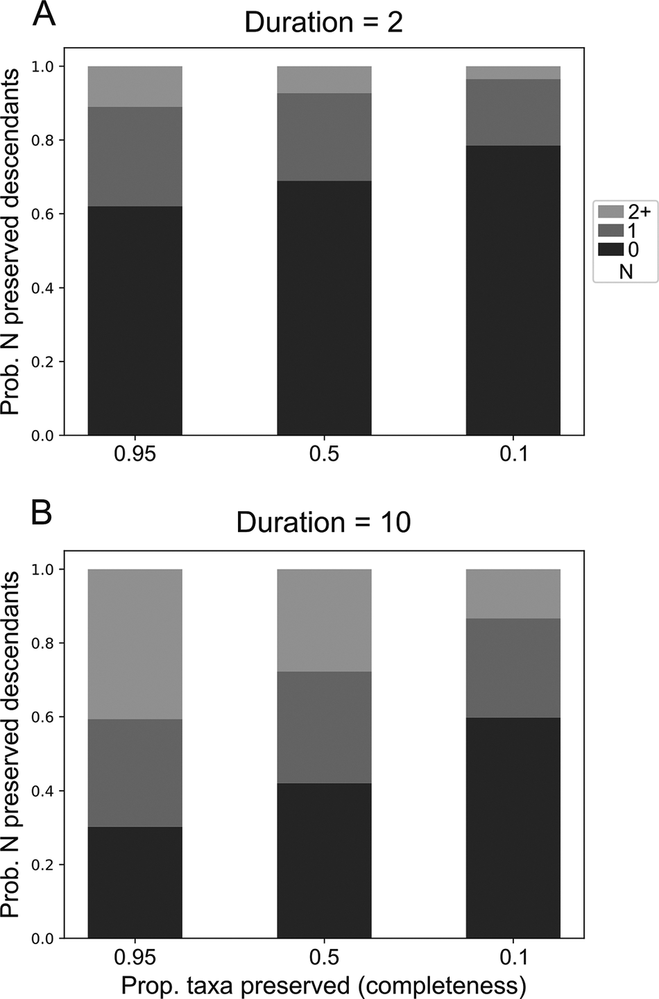
Under the model, taxa are expected to yield a distribution of sampled descendants. This distribution changes as a function of the duration of each taxon and the completeness of the fossil record. Taxa with longer durations belonging to clades with higher completeness are expected to give rise to more descendants (Fig. 2, Supplementary Figs. S6–S9). Accordingly, these taxa are the most likely candidates to be SSPs. Taxa with long durations (e.g., 10 Myr; Fig. 2B) should often be expected to yield multiple descendants, with even poorly preserved taxa having an almost 20% probability of giving rise to at least two sampled descendants.
Probability distribution of the number of sampled descendant clades stemming from a single ancestor with duration A, 2 and B, 10. Time units are arbitrary but were scaled to be approximately similar to millions of years for interpretability. Speciation (p) and extinction (q) rates were set to be equal at 0.1.

The Distribution of Super-progenitors
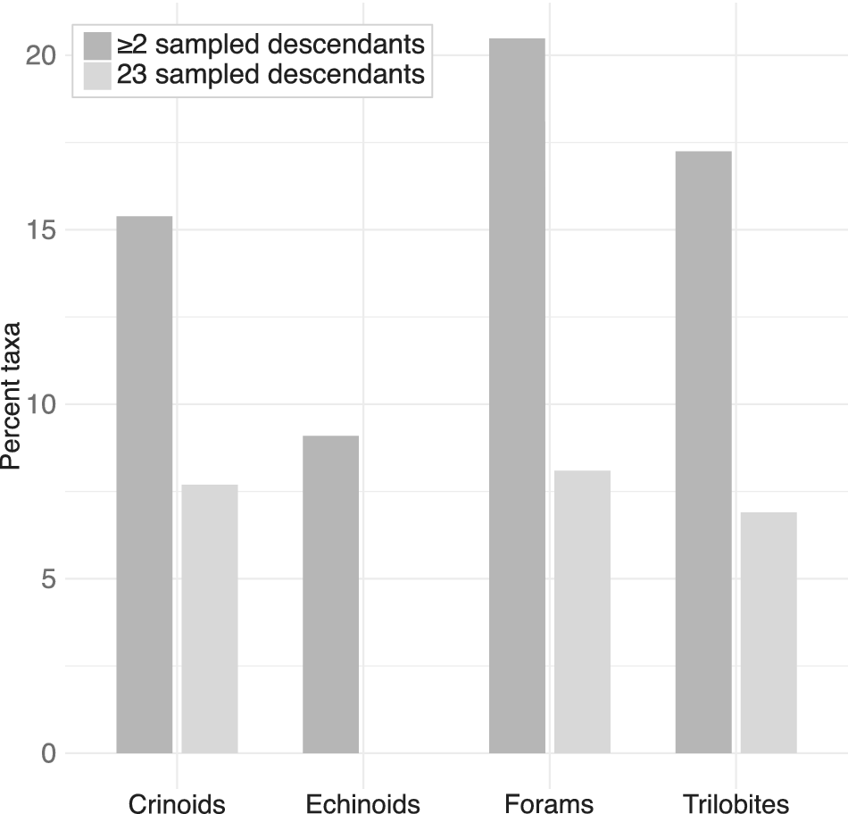
Visible super-progenitors should be common across almost all of the clades surveyed (Fig. 3). Based on the parameter estimates and observed stratigraphic ranges, across all of the clades at least 8% of taxa are expected under the model to give rise to at least two sampled descendants (2+ SSPs). For all clades but the echinoids, at least 7% of taxa are expected to give rise to at least three sampled descendants (3+ SSPs). While the expected proportion of super-progenitors was quite consistent across the crinoids, foraminifera, and trilobites, the echinoids differed in their pattern, with far fewer taxa expected to give rise to 2+ sampled descendants and none expected to give rise to 3+. It is possible that this difference could simply stem from stochastic variability in the distribution of taxon durations, considering that both echinoid clades examined were quite small. Nevertheless, as a general trend, visible super-progenitors should be broadly common across the clades examined here.
Percentage of taxa within each clade expected to give rise to two or more (dark gray) sampled descendants or three or more (light gray) sampled descendants under the birth–death-sampling (BDS) model, given fitted rates (origination, extinction, and fossil preservation) and inferred taxon durations.

The Effect of Incomplete Stratigraphic Sampling
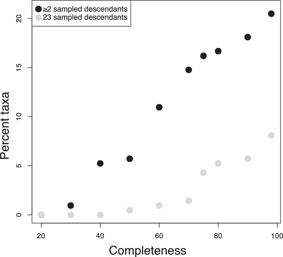
The clades examined here all displayed high completeness. Many clades across the fossil record cannot be expected to be preserved as thoroughly. To get a better sense of how often we might expect to encounter visible super-progenitors in less well-sampled clades, I investigated how the expected proportion varied as a function of the completeness of the fossil record. To accomplish this, I computed the proportion of super-progenitors expected under the BDS model in the foraminifera based on the inferred taxon durations (Supplementary fig. S10) and diversification parameters given in Table 1, while varying the stratigraphic sampling rate. I varied the sampling rate to achieve completeness values ranging from 20% to 100%. As long as the foraminiferan record is assumed to be at least 50% complete, >5% of taxa are expected to give rise to at least two sampled descendants and at least one taxon is expected to give rise to at least three sampled descendants (Fig. 4). The 2+ SSPs remain fairly common as long as at least 40% of taxa are preserved and only disappear entirely for records less than 30% complete.
Variation in the expected number of super-progenitors observed in the foraminifera dataset if the preservation rate is varied. If the fossil record is assumed to be particularly degraded (<40% complete), no taxa are expected to give rise to three or more sampled descendants, and few are expected to give rise to two or more. For fossil records at least 60% complete, super-progenitors are common enough to be an important factor in phylogenetic analyses and macroevolutionary patterns.

Variation in Turnover Rate and the Proportion of Super-progenitors
Because the proportion of visible super-progenitors is driven in large part by completeness, which is essentially calculated as a ratio of preservation rate to extinction rate, altering the extinction rate should be expected to yield similar patterns as varying the preservation rate, as was performed earlier. However, simply modifying completeness does not help us build intuition for how differences in the process of lineage diversification shapes patterns in the distribution of visible super-progenitors. Moreover, the procedure used earlier also ignores the effect of origination rate on this distribution. I sought to explore the interaction between the biological component of the model, captured by diversification rate, and the geological component, captured by preservation rate. There are two ways of approaching diversification rate in this context. One captures the overall “tempo” of diversification. This is captured by turnover, or the sum of origination and extinction rate. The other concerns the relative strength of origination and extinction. This is captured by net diversification rate. I modulated both in concert with preservation rates to develop a more comprehensive view of the interaction between these parameters.
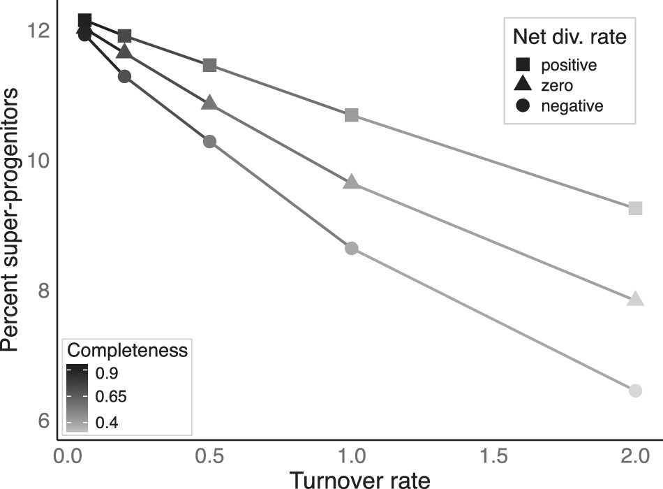
I found that, expectedly, the median percentage of 3+ SSPs declines as turnover rate is increased (Fig. 5). However, this decline happens quite slowly. As long as turnover rates fall within the range displayed by the empirical clades, the proportion of 3+ SSPs is quite high, falling between 11% and 12%. It takes an exceptionally high turnover rate of 1.0 to bring the expected proportion below 10%. There remains a fairly high proportion (6–10%) of 3+ SSPs even at the unrealistically high turnover rate of 2.0. It is likely that a large proportion of the variation in the proportion of SSPs stems from differences in completeness, similar to the foraminiferan results presented earlier. However, in contrast, these differences in completeness stem from variation in extinction rate, thus highlighting how elevated extinction contributes to patterns in SSPs. Some proportion of the observed differences also stem from variation in origination rate, however. This highlights how higher speciation rates will tend to lead to a greater proportion of SSPs as more descendants are generated and thus have a chance to enter the fossil record per unit time.
The median percentage of sampled super-progenitors (taxa with at least three sampled descendants) across replicate simulated clades as a function of turnover rate (origination rate + extinction rate). Preservation rate was set to 0.5 across all replicates. Completeness varied as a function of turnover rate. Clades were simulated with turnover rates of 0.06, 0.2, 0.5, 1.0, and 2.0. Values at the lower end of this range were close to the estimated turnover rates, while those at the higher end were unrealistically high, but were used to explore extreme cases, where super-progenitors would be least susceptible to being preserved as such. The relative contribution of origination and extinction to the overall turnover rate was altered to yield positive, net-zero, and negative net diversification rates.

Discussion
Under a wide range of biologically and geologically realistic parameterizations, the BDS model posits a wide distribution of the number of sampled descendants for each taxon. This distribution frequently predicts an impactful number of SSPs. These results demonstrate that super-progenitors are likely very common in the fossil record and that paleobiologists should expect to encounter them in many clades. This should open up both new challenges and new possibilities across analytical and phylogenetic paleobiology. Super-progenitors are accommodated by the mathematics of the FBDR model. However, many existing tree inference packages do not explicitly identify SSPs (especially those with at least three descendants). Nevertheless, increased recognition of their presence can spur the exploration of many exciting biological questions into the nature and shape of adaptive radiation and the patterns and mechanisms underlying speciation.
Implications for Phylogenetic Reconstruction
The ubiquity of super-progenitors has long been recognized by paleobiologists (Rensch Reference Rensch1959; Raup et al. Reference Raup, Gould, Schopf and Simberloff1973). Their prevalence is a basic theoretical expectation that stems from a birth–death model (Raup Reference Raup1985; Foote Reference Foote1996) but has been suggested empirically as well (Wagner and Erwin Reference Wagner, Erwin and Anstey1995). Despite this, few phylogenetic methods applied to fossil clades are equipped to search for them. The results presented here demonstrate that SSPs should be common, even after accounting for the effects of incomplete taxon sampling. And so, incorporating tree models and tree search routines that accommodate super-progenitors should become the standard in phylogenetic paleobiology. Phylogenies reconstructed from methods that fail to do so run a high risk of depicting misleading relationships, especially in well-preserved clades of organisms such as are found in the marine invertebrate fossil record. It should be noted that some existing methods accommodate for super-progenitors through the fossilized birth–death (FBD) prior but may produce trees that do not specify which taxon gave rise to multiple descendants (Stadler Reference Stadler2010). Devoting more attention to explicitly identifying SSPs could open new biological horizons by shedding light on the patterns and processes that give rise to new species.
The expansion of existing approaches to accommodate super-progenitors could be a boon for our understanding of phylogenetic relationships in many groups. Phylogenetic reconstruction in many clades often results in highly uncertain results and low resolution. It is possible that some of this uncertainty could be explained by current approaches’ attempts to force super-progenitors and their descendants into a set of bifurcating relationships. As a result, the biological insights gained by phylogenetic analyses of fossil clades could improve if super-progenitors are more routinely identified by existing algorithms. Previous mathematical limitations to recognizing super-progenitors stemmed from the lack of an explicit framework for incorporating full durations and stratigraphic ranges of fossil taxa. This hurdle has been overcome by the FBDR and related models (Stadler et al. Reference Stadler, Gavryushkina, Warnock, Drummond and Heath2018). The last existing barrier concerns the implementation of these models and further development of tree search algorithms that explicitly test trees that include super-progenitors. Progress is being made on these fronts (Parins-Fukuchi Reference Parins-Fukuchi2025; Stolz et al. Reference Stolz, Gavryushkina, Vaughan, Stadler and Allen2025), but broader adoption will be important. Our knowledge has gradually expanded to recognize that sampled ancestors are likely very common in many empirical phylogenetic trees (Foote Reference Foote1996; Pett and Heath Reference Pett, Heath, Scornavacca, Delsuc and Galtier2020; Parins-Fukuchi and Saulsbury Reference Parins-Fukuchi and Saulsbury2025). Expanding this knowledge to characterizing the kinds of ancestor–descendant arrangements we might expect to find can improve the detail with which we reconstruct phylogeny and, perhaps more interestingly, uncover increasingly complex and interesting biological patterns. Because SSPs, and sampled ancestors more broadly, are expected to be common in many clades, further developing methods that anticipate their abundance can only improve paleobiologists’ capacity to leverage the fossil record to yield compelling evolutionary insights.
There are circumstances where paleobiologists might prefer only a simple cladogram. However, the typical model of a fully bifurcating cladogram does not fit fossil clades that contain SSPs. When a single ancestor gives rise to many descendants, the corresponding isomorphic cladogram involves a multifurcation. This is because no pair of descendants is more closely related to one another, or the ancestor, than any other pair. The high frequency of super-progenitors found here shows that multifurcations should be expected when reconstructing cladograms in many (especially well-preserved) fossil lineages. This reality has long been recognized (Wagner and Erwin Reference Wagner, Erwin and Anstey1995), but the implications have seldom been fully heeded. In short, budding processes of speciation should lead to cladistic patterns that differ from the fully bifurcating ones entertained by most parsimony approaches. While solutions have been proposed to explicitly test multifurcations during Bayesian tree inference (Lewis et al. Reference Lewis, Holder and Holsinger2005), they have not been applied more broadly. This is especially the case for parsimony methods used to produce cladograms representing fossil clades. And so, the concerns outlined earlier for incorporating super-progenitors into reconstruction of phylogenetic trees also apply to cladograms, even though cladograms are not intended to be interpreted as phylogenetic trees.
BDS Models, SSPs, and Tests of Empirical Patterns
While the expectations presented here indicate a prevalence of SSPs in fossil clades, they do not assess the adequacy of the BDS model itself. Many recent approaches use models, often referred to as “fossilized birth–death” (FBD) process models, closely related to the BDS model employed here, as a Bayesian prior (Heath et al. Reference Heath, Huelsenbeck and Stadler2014). The basic parameters of the FBD model are the same as the model used here and elsewhere in the paleobiological literature, offering only several specific modifications to accommodate possible differences in topological structure in different trees, such as explicitly modeling distinct processes of budding and splitting cladogenesis (Stadler et al. Reference Stadler, Gavryushkina, Warnock, Drummond and Heath2018). Others have suggested the possibility of using BDS models as a primary means of phylogenetic inference in taxa that lack ample morphological data (Wagner Reference Wagner2019). I am enthusiastic about these developments and remain very optimistic about their utility to greatly advance paleobiologists’ ability to address important questions. If we wish to generate a stronger understanding of the empirical distribution of sampled descendants, it may also be useful to evaluate phylogenetic patterns without the statistical influence of the full BDS model. Such analyses could be performed using methods that are decoupled from any explicit model of the diversification process. Methods that incorporate stratigraphic range data and ancestor–descendant relationships but that do not include birth and death parameters could provide one way to begin exploration of the empirical frequency of SSPs independent of the BDS model (e.g., Fisher Reference Fisher, Grande and Rieppel1994; Alroy Reference Alroy1995; Wagner Reference Wagner1998; Parins-Fukuchi et al. Reference Parins-Fukuchi, Greiner, MacLatchy and Fisher2019; Parins-Fukuchi Reference Parins-Fukuchi2021). These approaches model the incomplete stratigraphic record, but do not incorporate explicit parameters that describe the lineage diversification process and so do not carry the same assumptions about the prevalence of super-progenitors. I suggest such approaches only as an additional tool that could be used to explore the patterns discussed here; BDS and FBDR models will undoubtedly and rightfully remain indispensable as phylogenetic approaches moving forward.
Impact of Sampling
SSPs are likely an important facet of phylogenetic patterns recovered in many well-sampled marine invertebrate clades. Empirical estimates of completeness in such clades are often well over 50%, often approaching and even exceeding 90% (Parins-Fukuchi and Saulsbury Reference Parins-Fukuchi and Saulsbury2025). As a result, it is likely important to accommodate the presence of super-progenitors when reconstructing phylogenies and/or macroevolutionary patterns in such clades. All of the clades studied here have very good fossil records. While super-progenitors should be common across the tree of life, their existence is likely obscured in many lineages with sparser records. So, while many of the implications discussed here likely remain relevant in such clades, they will probably need to be operationalized differently. Nevertheless, SSPs may still affect phylogenetic patterns even if they are not directly sampled. Multiple budding descendants from a shared super-progenitor can be sampled in extant clades, inducing multifurcations in the resulting topology (Parins-Fukuchi and Saulsbury Reference Parins-Fukuchi and Saulsbury2025). A similar effect could manifest in poorly sampled fossil clades. In this case, even if preservation in a clade is too low for a researcher to expect to encounter SSPs, the phylogenetic pattern induced by them may still need to be accounted for.
Turnover and SSPs
The simulation results show that, while turnover and net diversification rates have a marked impact on the structure of the phylogeny, diversification patterns alone are unlikely to reduce the occurrence of SSPs to a negligibly low level. Moreover, the simulations suggest that SSPs (especially those with at least three sampled descendants) may be especially important during episodes of explosive diversification, such as occur during adaptive radiation and during the early stages of the evolution of many clades. Clades undergoing such dynamics experience high net-diversification rates. This should, in turn, lead to a high proportion of 3+ SSPs. Such patterns have been documented in extant radiations. In the threespine sticklebacks, a widespread marine super-progenitor has repeatedly given rise to freshwater descendants (Schluter and McPhail Reference Schluter and McPhail1992). Such systems have yielded many fundamental insights into the ecological and evolutionary processes that mediate adaptive radiation. SSPs have also been widely identified in a variety of fossil clades using a range of phylogenetic methods (Wagner and Erwin Reference Wagner, Erwin and Anstey1995; Parins-Fukuchi Reference Parins-Fukuchi2025; Stolz et al. Reference Stolz, Gavryushkina, Vaughan, Stadler and Allen2025). If SSPs are as common as is suggested by the BDS model explored here, fossil clades may be leveraged to address similar questions, but over deeper timescales and across a wide range of organisms. Such a research program could greatly deepen our knowledge of the evolutionary mechanisms that give rise to the wealth of lineages and phenotypes observed across nature and throughout the fossil record. This possibility also highlights a way that the fossil record could offer unique, and heretofore unrealized, contributions to evolutionary theory.
Extensions and Alternative Diversification Models and Processes
The study undertaken here is only a first exploration. In addition to the BDS model explored here, there are alternatives that also predict the existence of super-progenitors. For example, the unified neutral theory of biodiversity (UNTB) also predicts both budding and super-progenitors (Hubbell Reference Hubbell2001). While the specific assumptions of that model may or may not be justified, the general approach of modeling lineage diversification in relation to population-level processes through individual-level modeling may provide an even greater understanding of the conditions under which we might expect to observe SSPs and the demographic processes that give rise to them. While, like the BDS model explored here, UNTB and related models also predict the presence of super-progenitors, they anticipate distinct patterns in the temporal distribution of ancestors and their descendants. The link between a species’ propensity to speciate and its abundance will lead to an uneven distribution of descendants throughout a species’ duration. This differs from the BDS model, which predicts that species are equally likely to speciate at any point in their existence. Further examination using UNTB and more sophisticated variants (e.g., Rosindell et al. Reference Rosindell, Harmon and Etienne2015) and improved data will help to determine how population-level mechanisms can shape patterns observed across species. Alternatively, there may be additional population- and/or individual-level models not mentioned here that might better explain patterns observed in the fossil record than the BDS expectations generated here.
Exploration of these ideas using some form of fossil abundance data could be one useful way to reveal the ecological processes that mediate diversification and the phylogenetic patterns that result. However, these data are quite difficult to collect. Fossil taxa with higher abundances tend to be more resistant to extinction and so should generally be longer lived (Harnik Reference Harnik2011; Payne et al. Reference Payne, Truebe, Nützel and Chang2011), but the link between abundance and species fecundity has not been explored. Wider geographic range also has been shown to correspond to longer lineage durations (Jablonski Reference Jablonski1986; Kiessling and Aberhan Reference Kiessling and Aberhan2007; Payne and Finnegan Reference Payne and Finnegan2007; Harnik et al. Reference Harnik, Simpson and Payne2012; Foote and Miller Reference Foote and Miller2013; Foote et al. Reference Foote, Ritterbush and Miller2016). Taxa with wider geographic ranges will also tend to have higher abundances for most of their existence. A next step could involve investigating the distribution of descendants in light of geographic range en route to exploring abundance directly.
Conclusions
The analyses here show that SSPs should be a common occurrence across fossil clades with reasonably high levels of preservation. Studying fossil clades in the manner outlined in this paper, but with more flexible, biologically informed models may help us to better grasp the underlying ecological and population processes regulating the formation and survival of new species in the fossil record. In the meantime, developing new phylogenetic approaches that accommodate super-progenitors will help facilitate the reconstruction of more accurate and meaningful phylogenetic trees and provide the starting point for deeper exploration of the diversification of fossil clades.
Acknowledgments
I would like to thank M. Ahmad-Gawel, M. Foote, F. Gahn, E. Hagen, D. L. Mahler, J. Pease, L. Rowe, J. Saulsbury, M. Su, G. W. Stull, and T. Wildeboer for conversations and criticisms that have greatly improved the article. I was supported by Natural Sciences and Engineering Research Council of Canada Discovery Grant RGPIN-2024-06289 during the course of this work.
Competing Interests
The author declares no conflicts of interest.
Data Availability Statement
Data used for the analyses here are available publicly on Figshare at https://doi.org/10.6084/m9.figshare.27351165.v2. Code implementing the equations described here is available in the “main_exp_desc.py” script maintained and hosted on GitHub (https://github.com/tomopfuku/stratoML). This repository is not static, but the analyses presented here were performed using the versions of the code in commit 5b2471e.


 Open access