


1 Introduction
Over 50 years ago Strassen [Reference Strassen40] discovered that the usual row-column method for multiplying $\mathbf {n}\times \mathbf {n}$
matrices, which uses
$\mathbf {n}\times \mathbf {n}$
matrices, which uses $O(\mathbf {n}^3)$
arithmetic operations, is not optimal by exhibiting an explicit algorithm to multiply matrices using
$O(\mathbf {n}^3)$
arithmetic operations, is not optimal by exhibiting an explicit algorithm to multiply matrices using $O(\mathbf {n}^{2.81})$
arithmetic operations. Ever since then, substantial efforts have been made to determine just how efficiently matrices may be multiplied. See any of [Reference Bürgisser, Clausen and Shokrollahi12, Reference Bläser8, Reference Landsberg31] for an overview. Matrix multiplication of
$O(\mathbf {n}^{2.81})$
arithmetic operations. Ever since then, substantial efforts have been made to determine just how efficiently matrices may be multiplied. See any of [Reference Bürgisser, Clausen and Shokrollahi12, Reference Bläser8, Reference Landsberg31] for an overview. Matrix multiplication of $\mathbf {n}\times {\boldsymbol \ell }$
matrices with
$\mathbf {n}\times {\boldsymbol \ell }$
matrices with ${\boldsymbol \ell }\times \mathbf {m}$
matrices is a bilinear map, that is, a tensor
${\boldsymbol \ell }\times \mathbf {m}$
matrices is a bilinear map, that is, a tensor $M_{\langle {\boldsymbol \ell },\mathbf {m},\mathbf {n}\rangle }\in \mathbb C^{{\boldsymbol \ell }\mathbf {m}}{\mathord { \otimes } } \mathbb C^{\mathbf {m}\mathbf {n}}{\mathord { \otimes } } \mathbb C^{\mathbf {n}{\boldsymbol \ell }}$
, and since 1980 [Reference Bini6], the primary complexity measure of the matrix multiplication tensor has been its border rank, which is defined as follows.
$M_{\langle {\boldsymbol \ell },\mathbf {m},\mathbf {n}\rangle }\in \mathbb C^{{\boldsymbol \ell }\mathbf {m}}{\mathord { \otimes } } \mathbb C^{\mathbf {m}\mathbf {n}}{\mathord { \otimes } } \mathbb C^{\mathbf {n}{\boldsymbol \ell }}$
, and since 1980 [Reference Bini6], the primary complexity measure of the matrix multiplication tensor has been its border rank, which is defined as follows.
A nonzero tensor $T\in \mathbb C^{\mathbf {a}}{\mathord { \otimes } } \mathbb C^{\mathbf {b}}{\mathord { \otimes } } \mathbb C^{\mathbf {c}}=:A{\mathord { \otimes } } B{\mathord { \otimes } } C$
has rank one if
$T\in \mathbb C^{\mathbf {a}}{\mathord { \otimes } } \mathbb C^{\mathbf {b}}{\mathord { \otimes } } \mathbb C^{\mathbf {c}}=:A{\mathord { \otimes } } B{\mathord { \otimes } } C$
has rank one if $T=a{\mathord { \otimes } } b{\mathord { \otimes } } c$
for some
$T=a{\mathord { \otimes } } b{\mathord { \otimes } } c$
for some $a\in A$
,
$a\in A$
, $b\in B$
,
$b\in B$
, $c\in C$
and the rank of T, denoted
$c\in C$
and the rank of T, denoted $\mathbf {R} (T)$
, is the smallest r such that T may be written as a sum of r rank one tensors. The border rank of T, denoted
$\mathbf {R} (T)$
, is the smallest r such that T may be written as a sum of r rank one tensors. The border rank of T, denoted $\underline {\mathbf {R}}(T)$
, is the smallest r such that T may be written as a limit of a sum of r rank one tensors. In geometric language, the border rank is smallest r such that
$\underline {\mathbf {R}}(T)$
, is the smallest r such that T may be written as a limit of a sum of r rank one tensors. In geometric language, the border rank is smallest r such that $[T]\in \sigma _r(\operatorname {\mathrm {Seg}}(\mathbb P A\times \mathbb P B\times \mathbb P C))$
. Here,
$[T]\in \sigma _r(\operatorname {\mathrm {Seg}}(\mathbb P A\times \mathbb P B\times \mathbb P C))$
. Here, $\sigma _r(\operatorname {\mathrm {Seg}}(\mathbb P A\times \mathbb P B\times \mathbb P C))$
denotes the r-th secant variety of the Segre variety of rank one tensors. For the relations between rank, border rank and other measures of complexity, see [Reference Bürgisser, Clausen and Shokrollahi12, Ch. 14-15].
$\sigma _r(\operatorname {\mathrm {Seg}}(\mathbb P A\times \mathbb P B\times \mathbb P C))$
denotes the r-th secant variety of the Segre variety of rank one tensors. For the relations between rank, border rank and other measures of complexity, see [Reference Bürgisser, Clausen and Shokrollahi12, Ch. 14-15].
Despite the vast literature on matrix multiplication, previous to this paper, the precise border rank of $M_{\langle {\boldsymbol \ell },\mathbf {m},\mathbf {n}\rangle }$
was known in exactly one nontrivial case, namely
$M_{\langle {\boldsymbol \ell },\mathbf {m},\mathbf {n}\rangle }$
was known in exactly one nontrivial case, namely $M_{\langle 2\rangle }=M_{\langle 222\rangle }$
[Reference Landsberg29]. We determine the border rank in two new cases,
$M_{\langle 2\rangle }=M_{\langle 222\rangle }$
[Reference Landsberg29]. We determine the border rank in two new cases, $M_{\langle 223\rangle }$
and
$M_{\langle 223\rangle }$
and $M_{\langle 233\rangle }$
. We prove new border rank lower bounds for
$M_{\langle 233\rangle }$
. We prove new border rank lower bounds for $M_{\langle 3\rangle }$
and two infinite sequences of new cases,
$M_{\langle 3\rangle }$
and two infinite sequences of new cases, $M_{\langle 2\mathbf {n}\mathbf {n}\rangle }$
and
$M_{\langle 2\mathbf {n}\mathbf {n}\rangle }$
and $M_{\langle 3\mathbf {n}\mathbf {n}\rangle }$
. Previous to this paper, there were no nontrivial lower bounds for these sequences. In fact, there were no nontrivial border rank lower bounds for any tensor in
$M_{\langle 3\mathbf {n}\mathbf {n}\rangle }$
. Previous to this paper, there were no nontrivial lower bounds for these sequences. In fact, there were no nontrivial border rank lower bounds for any tensor in $\mathbb C^{\mathbf {a}}{\mathord { \otimes } } \mathbb C^{\mathbf {a}}{\mathord { \otimes } } \mathbb C^{\mathbf {b}}$
, where
$\mathbb C^{\mathbf {a}}{\mathord { \otimes } } \mathbb C^{\mathbf {a}}{\mathord { \otimes } } \mathbb C^{\mathbf {b}}$
, where $\mathbf {b}>2\mathbf {a}$
other than Lickteig’s near trivial bound [Reference Lickteig37]
$\mathbf {b}>2\mathbf {a}$
other than Lickteig’s near trivial bound [Reference Lickteig37] $\underline {\mathbf {R}}(M_{\langle \mathbf {m},\mathbf {n},\mathbf {n}\rangle })\geq \mathbf {n}^2+1$
when
$\underline {\mathbf {R}}(M_{\langle \mathbf {m},\mathbf {n},\mathbf {n}\rangle })\geq \mathbf {n}^2+1$
when $\mathbf {m}<\mathbf {n}$
, (where the bound of
$\mathbf {m}<\mathbf {n}$
, (where the bound of $\mathbf {n}^2$
is trivial). We also determine the border rank of the
$\mathbf {n}^2$
is trivial). We also determine the border rank of the $3\times 3$
determinant considered as a tensor, which is important for proving upper bounds on the exponent of matrix multiplication as discussed below. See §1.2 below for precise statements.
$3\times 3$
determinant considered as a tensor, which is important for proving upper bounds on the exponent of matrix multiplication as discussed below. See §1.2 below for precise statements.
1.1 Methods/History
This paper deals exclusively with lower bounds (“complexity theory’s Waterloo” according to [Reference Arora and Barak5, Chap. 14]). For a history of upper bounds, see, for example, [Reference Bläser8, Reference Landsberg31].
Let $\sigma _r(\operatorname {\mathrm {Seg}}(\mathbb P A\times \mathbb P B\times \mathbb P C))$
denote the set of tensors of border rank at most r, which is called the r-th secant variety of the Segre variety. Previously, border rank lower bounds for tensors were primarily obtained by finding a polynomial vanishing on
$\sigma _r(\operatorname {\mathrm {Seg}}(\mathbb P A\times \mathbb P B\times \mathbb P C))$
denote the set of tensors of border rank at most r, which is called the r-th secant variety of the Segre variety. Previously, border rank lower bounds for tensors were primarily obtained by finding a polynomial vanishing on $\sigma _r(\operatorname {\mathrm {Seg}}(\mathbb P A\times \mathbb P B\times \mathbb P C))$
and then showing the polynomial is nonzero when evaluated on the tensor in question. These polynomials were found by reducing multilinear algebra to linear algebra [Reference Strassen41], and also exploiting the large symmetry group of
$\sigma _r(\operatorname {\mathrm {Seg}}(\mathbb P A\times \mathbb P B\times \mathbb P C))$
and then showing the polynomial is nonzero when evaluated on the tensor in question. These polynomials were found by reducing multilinear algebra to linear algebra [Reference Strassen41], and also exploiting the large symmetry group of $\sigma _r(\operatorname {\mathrm {Seg}}(\mathbb P A\times \mathbb P B\times \mathbb P C))$
to help find the polynomials [Reference Landsberg and Ottaviani35, Reference Landsberg and Ottaviani36]. Such methods are subject to barriers [Reference Efremenko, Garg, Oliveira and Wigderson18, Reference Gałązka21]; see [Reference Landsberg32, §2.2] for an overview. A technique allowing one to go slightly beyond the barriers was introduced in [Reference Landsberg and Michałek34]. The novelty there was, in addition to exploiting the symmetry group of
$\sigma _r(\operatorname {\mathrm {Seg}}(\mathbb P A\times \mathbb P B\times \mathbb P C))$
to help find the polynomials [Reference Landsberg and Ottaviani35, Reference Landsberg and Ottaviani36]. Such methods are subject to barriers [Reference Efremenko, Garg, Oliveira and Wigderson18, Reference Gałązka21]; see [Reference Landsberg32, §2.2] for an overview. A technique allowing one to go slightly beyond the barriers was introduced in [Reference Landsberg and Michałek34]. The novelty there was, in addition to exploiting the symmetry group of $\sigma _r(\operatorname {\mathrm {Seg}}(\mathbb P A\times \mathbb P B\times \mathbb P C))$
, to also exploit the symmetry group of the tensor one wanted to prove lower bounds on. This border substitution method of [Reference Landsberg and Michałek34] relied on first using the symmetry of the tensor to study its degenerations via the Normal Form Lemma 2.3, and then to use polynomials on the degeneration of the tensor.
$\sigma _r(\operatorname {\mathrm {Seg}}(\mathbb P A\times \mathbb P B\times \mathbb P C))$
, to also exploit the symmetry group of the tensor one wanted to prove lower bounds on. This border substitution method of [Reference Landsberg and Michałek34] relied on first using the symmetry of the tensor to study its degenerations via the Normal Form Lemma 2.3, and then to use polynomials on the degeneration of the tensor.
The classical apolarity method studies the decompositions of a homogeneous polynomial of degree d into a sum of d-th powers of linear forms, (these are called Waring rank decompositions); see,for example, [Reference Iarrobino and Kanev27]. It was generalized to study ranks of points with respect to toric varieties [Reference Gałązka22, Reference Gallet, Ranestad and Villamizar23]. To prove rank lower bounds with it, one takes the ideal of linear differential operators annihilating a given polynomial P and proves it does not contain an ideal annihilating r distinct points. In [Reference Buczyńska and Buczyński11], Buczyńska and Buczyński extend this classical method to the border rank setting. They also extend the Normal Form Lemma to the entire ideal associated to the border rank decomposition of the tensor, their Fixed Ideal Theorem (Theorem 2.4). (In the language introduced below, the Normal Form Lemma is the $(111)$
case of the Fixed Ideal Theorem.) In the present work, we describe an algorithm to enumerate a set of parameterized families of ideals which together exhaust those which could satisfy the conclusion of the Fixed Ideal Theorem, and we show this enumeration fails to produce any candidates in important cases of interest.
$(111)$
case of the Fixed Ideal Theorem.) In the present work, we describe an algorithm to enumerate a set of parameterized families of ideals which together exhaust those which could satisfy the conclusion of the Fixed Ideal Theorem, and we show this enumeration fails to produce any candidates in important cases of interest.
The ideals subject to enumeration are homogeneous in three sets of variables, so we have a $\mathbb {Z}^3$
-graded ring of polynomials, that is,
$\mathbb {Z}^3$
-graded ring of polynomials, that is, $I=\bigoplus _{i,j,k} I_{ijk}$
, and we may study a putative ideal I in each multidegree. Given r, the ideal enumeration algorithm builds a candidate ideal family step by step, starting in low (multi) degree and building upwards. At each building step, there are tests that restrict a so-far built family to a subfamily, and after these tests empty families are removed. If at any point there are no remaining candidates, one concludes there is no border rank r decomposition. For tensors with large symmetry groups, the dimensions of candidate ideal families one needs to consider during this enumeration are typically small. All the results of this paper require examining only the first few multigraded components of candidate ideal families.
$I=\bigoplus _{i,j,k} I_{ijk}$
, and we may study a putative ideal I in each multidegree. Given r, the ideal enumeration algorithm builds a candidate ideal family step by step, starting in low (multi) degree and building upwards. At each building step, there are tests that restrict a so-far built family to a subfamily, and after these tests empty families are removed. If at any point there are no remaining candidates, one concludes there is no border rank r decomposition. For tensors with large symmetry groups, the dimensions of candidate ideal families one needs to consider during this enumeration are typically small. All the results of this paper require examining only the first few multigraded components of candidate ideal families.
The restrictions to subfamilies result from upper bounding the ranks of certain linear maps. The linear maps are multiplication maps. On one hand, in order for a candidate space of polynomials to be an ideal, it must be closed under multiplication. On the other hand, our hypothesis that the ideal arises via a border rank r decomposition upper-bounds its dimension in each nontrivial multidegree; in fact one may assume it has codimension r in each multidegree.
The fact that the elimination conditions are rank conditions implies that the lower bound barriers [Reference Efremenko, Garg, Oliveira and Wigderson18, Reference Gałązka21] still hold for the technique as presented in this paper. In §1.3, we explain how we plan to augment these tests to go beyond the barriers in future work and how our techniques might be used to overcome upper bound barriers for the laser method as well.
We use representation theory at several levels. For tensors with symmetry, the Fixed Ideal Theorem significantly restricts the candidate $I_{ijk}$
’s one must consider, namely to those that are fixed by a Borel subgroup of the symmetry group of the tensor. Without this additional condition, even low degree ideal enumeration would likely be impossible to carry out except for very small examples.
$I_{ijk}$
’s one must consider, namely to those that are fixed by a Borel subgroup of the symmetry group of the tensor. Without this additional condition, even low degree ideal enumeration would likely be impossible to carry out except for very small examples.
We also make standard use of representation theory to put the matrices whose ranks we need to lower-bound in block diagonal format via Schur’s lemma. For example, to prove $\underline {\mathbf {R}}(M_{\langle 2\rangle })>6$
, the border apolarity method produces three size
$\underline {\mathbf {R}}(M_{\langle 2\rangle })>6$
, the border apolarity method produces three size $40\times 40$
matrices whose ranks need to be lower bounded. Decomposing the matrices to maps between isotypic components reduces the calculation to computing the ranks of several matrices of size
$40\times 40$
matrices whose ranks need to be lower bounded. Decomposing the matrices to maps between isotypic components reduces the calculation to computing the ranks of several matrices of size $4\times 8$
with entries
$4\times 8$
with entries $0,\pm 1$
, making the proof easily hand-checkable.
$0,\pm 1$
, making the proof easily hand-checkable.
Our results for $M_{\langle 3\rangle }$
and
$M_{\langle 3\rangle }$
and $\operatorname {det}_3$
are obtained by a computer implementation of the ideal enumeration algorithm.
$\operatorname {det}_3$
are obtained by a computer implementation of the ideal enumeration algorithm.
For $M_{\langle 2\mathbf {n}\mathbf {n}\rangle }$
and
$M_{\langle 2\mathbf {n}\mathbf {n}\rangle }$
and $M_{\langle 3\mathbf {n}\mathbf {n}\rangle }$
, we must handle all
$M_{\langle 3\mathbf {n}\mathbf {n}\rangle }$
, we must handle all $\mathbf {n}$
uniformly, and a computer calculation is no longer possible. To do this, we consider potential
$\mathbf {n}$
uniformly, and a computer calculation is no longer possible. To do this, we consider potential $I_{110}$
candidates as a certain sum of ‘local’ contributions, which we analyze separately (Lemmas 7.2 and 7.4). Given this analysis, it is possible to give a purely combinatorial necessary condition for the suitability of a potential
$I_{110}$
candidates as a certain sum of ‘local’ contributions, which we analyze separately (Lemmas 7.2 and 7.4). Given this analysis, it is possible to give a purely combinatorial necessary condition for the suitability of a potential $I_{110}$
candidate, and the analysis of all potential candidates then takes the form of a combinatorial optimization problem over filled Young diagrams (Lemma 7.7). This technique reduces the problem to checking three cases of local contribution for
$I_{110}$
candidate, and the analysis of all potential candidates then takes the form of a combinatorial optimization problem over filled Young diagrams (Lemma 7.7). This technique reduces the problem to checking three cases of local contribution for $M_{\langle 2\mathbf {n}\mathbf {n}\rangle }$
and eight cases for
$M_{\langle 2\mathbf {n}\mathbf {n}\rangle }$
and eight cases for $M_{\langle 3\mathbf {n}\mathbf {n}\rangle }$
. This method for proving lower bounds is completely different from previous techniques.
$M_{\langle 3\mathbf {n}\mathbf {n}\rangle }$
. This method for proving lower bounds is completely different from previous techniques.
To enable a casual reader to see the various techniques we employ, we return to the proof that $\underline {\mathbf {R}}(M_{\langle 2\rangle })>6$
multiple times: first using the general algorithm naïvely in §4, then working dually to reduce the calculation (Remark 4.1), then using representation theory to block diagonalize the calculation in §6.2 and finally we observe that the result is an immediate consequence of our localization principle and Lemma 7.2 (Remark 7.3).
$\underline {\mathbf {R}}(M_{\langle 2\rangle })>6$
multiple times: first using the general algorithm naïvely in §4, then working dually to reduce the calculation (Remark 4.1), then using representation theory to block diagonalize the calculation in §6.2 and finally we observe that the result is an immediate consequence of our localization principle and Lemma 7.2 (Remark 7.3).
1.2 Results
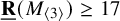
Theorem 1.1. $\underline {\mathbf {R}}(M_{\langle 3\rangle })\geq 17$
.
$\underline {\mathbf {R}}(M_{\langle 3\rangle })\geq 17$
.
The previous lower bounds were $14$
[Reference Strassen41] in 1983,
$14$
[Reference Strassen41] in 1983, $15$
[Reference Landsberg and Ottaviani36] in 2015 and
$15$
[Reference Landsberg and Ottaviani36] in 2015 and $16$
[Reference Landsberg and Michałek34] in 2018.
$16$
[Reference Landsberg and Michałek34] in 2018.
Let $\operatorname {det}_3\in \mathbb C^9{\mathord { \otimes } } \mathbb C^9{\mathord { \otimes } } \mathbb C^9$
denote the
$\operatorname {det}_3\in \mathbb C^9{\mathord { \otimes } } \mathbb C^9{\mathord { \otimes } } \mathbb C^9$
denote the $3\times 3$
determinant polynomial considered as a tensor. That is, as a bilinear map, it inputs two
$3\times 3$
determinant polynomial considered as a tensor. That is, as a bilinear map, it inputs two $3\times 3$
matrices and returns a third such that if the input is
$3\times 3$
matrices and returns a third such that if the input is $(M,M)$
, the output is the cofactor matrix of M.
$(M,M)$
, the output is the cofactor matrix of M.
Strassen’s laser method [Reference Strassen39] upper bounds the exponent of matrix multiplication using “simple” tensors. In [Reference Alman and Vassilevska Williams2, Reference Alman and Vassilevska Williams3, Reference Alman1, Reference Christandl, Vrana and Zuiddam13], barriers to proving further upper bounds with the method were found for many tensors. In [Reference Conner, Gesmundo, Landsberg and Ventura15], we showed that the (unique up to scale) skew-symmetric tensor in $\mathbb C^3{\mathord { \otimes } } \mathbb C^3{\mathord { \otimes } } \mathbb C^3$
, which we denote
$\mathbb C^3{\mathord { \otimes } } \mathbb C^3{\mathord { \otimes } } \mathbb C^3$
, which we denote $T_{skewcw,2}$
, is not subject to these upper bound barriers and could potentially be used to prove the exponent of matrix multiplication is two via its Kronecker powers. Explicitly, if one were to prove that
$T_{skewcw,2}$
, is not subject to these upper bound barriers and could potentially be used to prove the exponent of matrix multiplication is two via its Kronecker powers. Explicitly, if one were to prove that $\lim _{k{\mathord {\;\rightarrow \;}}\infty } \underline {\mathbf {R}}(T_{skewcw,2}^{\boxtimes k})^{\frac 1k}$
equals
$\lim _{k{\mathord {\;\rightarrow \;}}\infty } \underline {\mathbf {R}}(T_{skewcw,2}^{\boxtimes k})^{\frac 1k}$
equals $3$
, that would imply the exponent is two. One has
$3$
, that would imply the exponent is two. One has $\underline {\mathbf {R}}(T_{skewcw,2})=5$
and
$\underline {\mathbf {R}}(T_{skewcw,2})=5$
and $T_{skewcw,2}^{\boxtimes 2}=\operatorname {det}_3$
; see [Reference Conner, Gesmundo, Landsberg and Ventura15]. Thus, the following result is important for matrix multiplication complexity upper bounds:
$T_{skewcw,2}^{\boxtimes 2}=\operatorname {det}_3$
; see [Reference Conner, Gesmundo, Landsberg and Ventura15]. Thus, the following result is important for matrix multiplication complexity upper bounds:
Theorem 1.2. $\underline {\mathbf {R}}(\operatorname {det}_3)= 17$
.
$\underline {\mathbf {R}}(\operatorname {det}_3)= 17$
.
The upper bound was proved in [Reference Conner, Gesmundo, Landsberg and Ventura15]. In [Reference Boij and Teitler9], a lower bound of $15$
for the Waring rank of
$15$
for the Waring rank of $\operatorname {det}_3$
was proven. The previous border rank lower bound was
$\operatorname {det}_3$
was proven. The previous border rank lower bound was $12$
as discussed in [Reference Farnsworth19], which follows from the Koszul flattening equations [Reference Landsberg and Ottaviani36]. Note that had the result here turned out differently, for example, were the border rank
$12$
as discussed in [Reference Farnsworth19], which follows from the Koszul flattening equations [Reference Landsberg and Ottaviani36]. Note that had the result here turned out differently, for example, were the border rank $16$
or lower,
$16$
or lower, $T_{skewcw,2}$
would have immediately been promoted to the most promising tensor for proving the exponent is two; see the discussion in [Reference Conner, Gesmundo, Landsberg and Ventura15].
$T_{skewcw,2}$
would have immediately been promoted to the most promising tensor for proving the exponent is two; see the discussion in [Reference Conner, Gesmundo, Landsberg and Ventura15].
Remark 1.3. The computation of the trilinear map associated to $\operatorname {det}_3$
, which inputs three matrices and outputs a number, is different than the computation of the associated polynomial, which inputs a single matrix and outputs a number. The polynomial may be computed using
$\operatorname {det}_3$
, which inputs three matrices and outputs a number, is different than the computation of the associated polynomial, which inputs a single matrix and outputs a number. The polynomial may be computed using $12$
multiplications in the naïve algorithm and using
$12$
multiplications in the naïve algorithm and using $10$
with the algorithm in [Reference Derksen17].
$10$
with the algorithm in [Reference Derksen17].
Previous to this paper, $M_{\langle 2\rangle }$
was the only nontrivial matrix multiplication tensor whose border rank had been determined, despite
$M_{\langle 2\rangle }$
was the only nontrivial matrix multiplication tensor whose border rank had been determined, despite $50$
years of work on the subject. We add two more cases to this list.
$50$
years of work on the subject. We add two more cases to this list.
Theorem 1.4. $\underline {\mathbf {R}}(M_{\langle 223\rangle })=10$
.
$\underline {\mathbf {R}}(M_{\langle 223\rangle })=10$
.
The upper bound dates back to Bini et al. in 1980 [Reference Bini, Lotti and Romani7]. Koszul flattenings [Reference Landsberg and Ottaviani36] give $\underline {\mathbf {R}}(M_{\langle 22\mathbf {n}\rangle })\geq 3\mathbf {n}$
. Smirnov [Reference Smirnov38] showed that
$\underline {\mathbf {R}}(M_{\langle 22\mathbf {n}\rangle })\geq 3\mathbf {n}$
. Smirnov [Reference Smirnov38] showed that $\underline {\mathbf {R}}(M_{\langle 22\mathbf {n}\rangle })\leq 3\mathbf {n}+1$
for
$\underline {\mathbf {R}}(M_{\langle 22\mathbf {n}\rangle })\leq 3\mathbf {n}+1$
for $\mathbf {n}\leq 7$
, and we expect equality to hold for all
$\mathbf {n}\leq 7$
, and we expect equality to hold for all $\mathbf {n}$
.
$\mathbf {n}$
.
Theorem 1.5.
-
1.
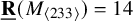
 $\underline {\mathbf {R}}(M_{\langle 233\rangle })=14$
.
$\underline {\mathbf {R}}(M_{\langle 233\rangle })=14$
. -
2. We have the following border rank lower bounds:
$$ \begin{align*} \mathbf{n} &\quad \underline{\mathbf{R}}(M_{\langle 2\mathbf{n}\mathbf{n}\rangle})\geq & \mathbf{n} &\quad \underline{\mathbf{R}}(M_{\langle 2\mathbf{n}\mathbf{n}\rangle})\geq & \mathbf{n} &\quad \underline{\mathbf{R}}(M_{\langle 2\mathbf{n}\mathbf{n}\rangle})\geq \\ 4 & \quad 22=4^2+6 & 11 & \quad 136=11^2+15 & 18 & \quad 348= 18^2+24 \\ 5 & \quad 32=5^2+7 & 12 & \quad 161=12^2+17 & 19 & \quad 387=19^2+26 \\ 6 & \quad 44=6^2+8 & 13 & \quad 187=13^2+18 & 20 & \quad 427= 20^2+27 \\ 7 & \quad 58=7^2+9 & 14 & \quad 215=14^2+19 & 21 & \quad 470= 21^2+29 \\ 8 & \quad 75=8^2+11 & 15 & \quad 246=15^2+21 & 22 & \quad 514= 22^2+30 \\ 9 & \quad 93=9^2+12 & 16 & \quad 278=16^2+22 & 23 & \quad 561= 23^2+32 \\ 10 & \quad 114=10^2+14 & 17 & \quad 312=17^2+23 & 24 & \quad 609= 24^2+33. \end{align*} $$
-
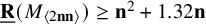
3. For
$0 < \epsilon < \frac {1}{4}$
, and
$\mathbf {n}>\frac {6}{\epsilon } \frac {3\sqrt {6}+6 - \epsilon }{6\sqrt {6} - \epsilon }$
,
$\underline {\mathbf {R}}(M_{\langle 2\mathbf {n}\mathbf {n}\rangle })\geq \mathbf {n}^2+(3\sqrt {6}-6-\epsilon ) \mathbf {n} $
. In particular,
$\underline {\mathbf {R}}(M_{\langle 2\mathbf {n}\mathbf {n}\rangle })\geq \mathbf {n}^2+1.32 \mathbf {n}+1$
when
$\mathbf {n}\geq 25$
.


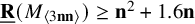
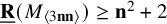
Previously, only the near trivial result that $\underline {\mathbf {R}}(M_{\langle 2\mathbf {n}\mathbf {n}\rangle })\geq \mathbf {n}^2+1$
was known by [Reference Lickteig37, Rem. p175].
$\underline {\mathbf {R}}(M_{\langle 2\mathbf {n}\mathbf {n}\rangle })\geq \mathbf {n}^2+1$
was known by [Reference Lickteig37, Rem. p175].
The upper bound in (1) is due to Smirnov [Reference Smirnov38], where he also proved $\underline {\mathbf {R}}(M_{\langle 244\rangle })\leq 24$
, and
$\underline {\mathbf {R}}(M_{\langle 244\rangle })\leq 24$
, and $ \underline {\mathbf {R}}(M_{\langle 255\rangle })\leq 38$
. When
$ \underline {\mathbf {R}}(M_{\langle 255\rangle })\leq 38$
. When $\mathbf {n}$
is even, one has the upper bound
$\mathbf {n}$
is even, one has the upper bound $\underline {\mathbf {R}}(M_{\langle 2\mathbf {n}\mathbf {n}\rangle })\leq \frac 74\mathbf {n}^2$
by writing
$\underline {\mathbf {R}}(M_{\langle 2\mathbf {n}\mathbf {n}\rangle })\leq \frac 74\mathbf {n}^2$
by writing $M_{\langle 2\mathbf {n}\mathbf {n}\rangle }=M_{\langle 222\rangle }\boxtimes M_{\langle 1\frac {\mathbf {n}}{2}\frac {\mathbf {n}}{2}\rangle }$
, where
$M_{\langle 2\mathbf {n}\mathbf {n}\rangle }=M_{\langle 222\rangle }\boxtimes M_{\langle 1\frac {\mathbf {n}}{2}\frac {\mathbf {n}}{2}\rangle }$
, where $\boxtimes $
denotes Kronecker product of tensors; see, for example, [Reference Conner, Gesmundo, Landsberg and Ventura15].
$\boxtimes $
denotes Kronecker product of tensors; see, for example, [Reference Conner, Gesmundo, Landsberg and Ventura15].
Theorem 1.6. For all $\mathbf {n}\ge 18$
,
$\mathbf {n}\ge 18$
, $\underline {\mathbf {R}}(M_{\langle 3\mathbf {n}\mathbf {n}\rangle })\geq \mathbf {n}^2+\sqrt {\frac 83} \mathbf {n}> \mathbf {n}^2+1.6\mathbf {n} $
.
$\underline {\mathbf {R}}(M_{\langle 3\mathbf {n}\mathbf {n}\rangle })\geq \mathbf {n}^2+\sqrt {\frac 83} \mathbf {n}> \mathbf {n}^2+1.6\mathbf {n} $
.
Previously, the only bound was the near trivial result that when $\mathbf {n}\geq 4$
,
$\mathbf {n}\geq 4$
, $\underline {\mathbf {R}}(M_{\langle 3\mathbf {n}\mathbf {n}\rangle })\geq \mathbf {n}^2+2$
by [Reference Lickteig37, Rem. p175].
$\underline {\mathbf {R}}(M_{\langle 3\mathbf {n}\mathbf {n}\rangle })\geq \mathbf {n}^2+2$
by [Reference Lickteig37, Rem. p175].
Using [Reference Lickteig37, Rem. p175], one obtains:
Corollary 1.7. For all $\mathbf {n} \ge 18$
and
$\mathbf {n} \ge 18$
and $\mathbf {m}\geq 3$
,
$\mathbf {m}\geq 3$
, $\underline {\mathbf {R}}(M_{\langle \mathbf {m}\mathbf {n}\mathbf {n}\rangle })\ge \mathbf {n}^2+\sqrt {\frac 83} \mathbf {n} +\mathbf {m}-3$
.
$\underline {\mathbf {R}}(M_{\langle \mathbf {m}\mathbf {n}\mathbf {n}\rangle })\ge \mathbf {n}^2+\sqrt {\frac 83} \mathbf {n} +\mathbf {m}-3$
.
Theorems 1.5 and 1.6 are the first nontrivial border rank lower bounds for any tensor in $\mathbb C^{\mathbf {a}}{\mathord { \otimes } } \mathbb C^{\mathbf {b}}{\mathord { \otimes } } \mathbb C^{\mathbf {c}}$
when
$\mathbb C^{\mathbf {a}}{\mathord { \otimes } } \mathbb C^{\mathbf {b}}{\mathord { \otimes } } \mathbb C^{\mathbf {c}}$
when $\mathbf {c}>2\operatorname {max}\{ \mathbf {a},\mathbf {b}\}$
other than the above mentioned near trivial result of Lickteig, vastly expanding the classes of tensors for which lower bound techniques exist.
$\mathbf {c}>2\operatorname {max}\{ \mathbf {a},\mathbf {b}\}$
other than the above mentioned near trivial result of Lickteig, vastly expanding the classes of tensors for which lower bound techniques exist.
1.3 What comes next?
1.3.1 Breaking the lower bound barriers
The geometric interpretation of the border rank lower bound barriers of [Reference Efremenko, Garg, Oliveira and Wigderson18, Reference Gałązka21] is that all equations obtained by taking minors, called rank methods, are actually equations for a larger variety than $\sigma _r(\operatorname {\mathrm {Seg}}(\mathbb P A\times \mathbb P B\times \mathbb P C))$
, called the r-th cactus variety [Reference Buczyńska and Buczyński11]. This cactus variety agrees with the secant variety for
$\sigma _r(\operatorname {\mathrm {Seg}}(\mathbb P A\times \mathbb P B\times \mathbb P C))$
, called the r-th cactus variety [Reference Buczyńska and Buczyński11]. This cactus variety agrees with the secant variety for $r<13$
, but it quickly fills the ambient space of tensors in
$r<13$
, but it quickly fills the ambient space of tensors in $\mathbb C^{\mathbf {m}}{\mathord { \otimes } }\mathbb C^{\mathbf {m}}{\mathord { \otimes } } \mathbb C^{\mathbf {m}}$
at latest when
$\mathbb C^{\mathbf {m}}{\mathord { \otimes } }\mathbb C^{\mathbf {m}}{\mathord { \otimes } } \mathbb C^{\mathbf {m}}$
at latest when $r=6\mathbf {m}-4$
. Thus one cannot prove
$r=6\mathbf {m}-4$
. Thus one cannot prove $\underline {\mathbf {R}}(T)>6\mathbf {m}-4$
for any tensor T via rank/determinantal methods, in particular, with border apolarity alone.
$\underline {\mathbf {R}}(T)>6\mathbf {m}-4$
for any tensor T via rank/determinantal methods, in particular, with border apolarity alone.
In brief, the r-th secant variety consists of points on limits of spans of zero-dimensional smooth schemes of length r. The r-th cactus variety consists of points on limits of spans of zero-dimensional schemes of length r.
The border apolarity algorithm produces ideals, and thus to break the barrier, one needs to distinguish ideals that are limits of smooth schemes from ideals that are limits of nonsmoothable schemes, and ideals that are not limits of any sequence of saturated ideals. In principle, this can be done using deformation theory (see, e.g., [Reference Hartshorne25]). This is exciting, as it is the first proposed path to overcoming the lower bound barriers.
Remark 1.8. After this paper was posted on arXiv, we went on to find an ideal passing all border apolarity tests for $M_{\langle 3\rangle }$
with
$M_{\langle 3\rangle }$
with $r=17$
. We are currently working to effectively implement deformation theory to determine if such an example comes from an actual border rank
$r=17$
. We are currently working to effectively implement deformation theory to determine if such an example comes from an actual border rank $17$
decomposition. The obstruction to doing this is the effective implementation of the theory. The naïve implementation, even on a large computer cluster, is not feasible, and we are working to develop effective computational techniques.
$17$
decomposition. The obstruction to doing this is the effective implementation of the theory. The naïve implementation, even on a large computer cluster, is not feasible, and we are working to develop effective computational techniques.
1.3.2 Upper bounds, especially for tensors relevant for Strassen’s laser method
There is intense interest in tensors not subject to the upper bound barriers for Strassen’s laser method described in [Reference Ambainis, Filmus and Le Gall4, Reference Alman1, Reference Alman and Vassilevska Williams3, Reference Christandl, Vrana and Zuiddam13]. All tensors used in or proposed for the laser method have positive-dimensional symmetry groups, so the border apolarity method potentially may be applied. For example, the small Coppersmith–Winograd tensor $T_{cw,q}:=\sum _{j=1}^q a_0{\mathord { \otimes } } b_j{\mathord { \otimes } } c_j+ a_j{\mathord { \otimes } } b_0{\mathord { \otimes } } c_j+ a_j{\mathord { \otimes } } b_j{\mathord { \otimes } } c_0$
has a very large symmetry group, namely the orthogonal group
$T_{cw,q}:=\sum _{j=1}^q a_0{\mathord { \otimes } } b_j{\mathord { \otimes } } c_j+ a_j{\mathord { \otimes } } b_0{\mathord { \otimes } } c_j+ a_j{\mathord { \otimes } } b_j{\mathord { \otimes } } c_0$
has a very large symmetry group, namely the orthogonal group $O(q)$
[Reference Conner, Gesmundo, Landsberg and Ventura14], which has dimension
$O(q)$
[Reference Conner, Gesmundo, Landsberg and Ventura14], which has dimension $\binom q2$
. Since these tensors, and their Kronecker squares tend to have border rank below the cactus barrier, we expect to be able to effectively apply the method as is to determine the border rank at least for small Kronecker powers. After this paper was posted on arXiv, border apolarity was utilized to determine the border rank of
$\binom q2$
. Since these tensors, and their Kronecker squares tend to have border rank below the cactus barrier, we expect to be able to effectively apply the method as is to determine the border rank at least for small Kronecker powers. After this paper was posted on arXiv, border apolarity was utilized to determine the border rank of $T_{cw,2}^{\boxtimes 2}$
in [Reference Conner, Huang and Landsberg16] and the answer ended up being the known upper bound. We are developing techniques to write down usual border rank decompositions guided by the ideals produced by border apolarity to potentially determine new upper bounds for higher Kronecker powers of
$T_{cw,2}^{\boxtimes 2}$
in [Reference Conner, Huang and Landsberg16] and the answer ended up being the known upper bound. We are developing techniques to write down usual border rank decompositions guided by the ideals produced by border apolarity to potentially determine new upper bounds for higher Kronecker powers of $T_{cw,2}$
and
$T_{cw,2}$
and $\operatorname {det}_3$
(or to show that the known bounds are sharp). In other words, we are working to use border apolarity to inject some “science” into the “art” of finding upper bounds.
$\operatorname {det}_3$
(or to show that the known bounds are sharp). In other words, we are working to use border apolarity to inject some “science” into the “art” of finding upper bounds.
1.3.3 Geometrization of the
$(111)$
test for matrix multiplication

Our results for $M_{\langle 2\mathbf {n}\mathbf {n}\rangle },M_{\langle 3\mathbf {n}\mathbf {n}\rangle }$
for general
$M_{\langle 2\mathbf {n}\mathbf {n}\rangle },M_{\langle 3\mathbf {n}\mathbf {n}\rangle }$
for general $\mathbf {n}$
only use the
$\mathbf {n}$
only use the $(210)$
and
$(210)$
and $(120)$
tests as defined in §3, and we expect to be able to prove stronger results for general
$(120)$
tests as defined in §3, and we expect to be able to prove stronger results for general $\mathbf {n}$
in these cases once we develop a proper geometric understanding of the
$\mathbf {n}$
in these cases once we develop a proper geometric understanding of the $(111)$
test like we have for the
$(111)$
test like we have for the $(210)$
test.
$(210)$
test.
1.4 Overview
In §2, we review terminology regarding border rank decompositions of tensors, Borel subgroups and Borel fixed subspaces. We then describe a curve of multigraded ideals one may associate to a border rank decomposition. We also review Borel fixed subspaces and list them in the cases relevant for this paper. In §3, we describe the border apolarity algorithm and accompanying tests. In §4, we review the matrix multiplication tensor. In §5, we describe the computation to prove Theorems 1.1 and 1.2, which are computer assisted calculations, the code for which is available at github.com/adconner/chlbapolar. In §6, we discuss representation theory relevant for applying the border apolarity algorithm to matrix multiplication. In §7, we prove our localization and optimization algorithm and use it to prove Theorems 1.4, 1.5 and 1.6.
2 Preliminaries
2.1 Definitions/Notation
Throughout, $A,B,C,U,V,W$
will denote complex vector spaces, respectively, of dimensions
$A,B,C,U,V,W$
will denote complex vector spaces, respectively, of dimensions $\mathbf {a},\mathbf {b},\mathbf {c},\mathbf {u},\mathbf {v},\mathbf {w}$
. The dual space to A is denoted
$\mathbf {a},\mathbf {b},\mathbf {c},\mathbf {u},\mathbf {v},\mathbf {w}$
. The dual space to A is denoted $A^*$
. The space of symmetric degree d tensors is denoted
$A^*$
. The space of symmetric degree d tensors is denoted $S^dA$
, which may also be viewed as the space of degree d homogeneous polynomials on
$S^dA$
, which may also be viewed as the space of degree d homogeneous polynomials on $A^*$
. Set
$A^*$
. Set $\operatorname {Sym}(A):=\bigoplus _d S^dA$
. The identity map is denoted
$\operatorname {Sym}(A):=\bigoplus _d S^dA$
. The identity map is denoted $\operatorname {Id}_A\in A{\mathord { \otimes } } A^*$
. For
$\operatorname {Id}_A\in A{\mathord { \otimes } } A^*$
. For $X\subset A$
,
$X\subset A$
, $X^{\perp }:=\{\alpha \in A^*\mid \alpha (x)=0, \forall x\in X\}$
is its annihilator, and
$X^{\perp }:=\{\alpha \in A^*\mid \alpha (x)=0, \forall x\in X\}$
is its annihilator, and $\langle X\rangle \subset A$
denotes the linear span of X. Projective space is
$\langle X\rangle \subset A$
denotes the linear span of X. Projective space is $\mathbb P A= (A\backslash \{0\})/\mathbb C^*$
, and if
$\mathbb P A= (A\backslash \{0\})/\mathbb C^*$
, and if $x\in A\backslash \{0\}$
, we let
$x\in A\backslash \{0\}$
, we let $[x]\in \mathbb P A$
denote the associated point in projective space (the line through x). The general linear group of invertible linear maps
$[x]\in \mathbb P A$
denote the associated point in projective space (the line through x). The general linear group of invertible linear maps $A{\mathord {\;\rightarrow \;}} A$
is denoted
$A{\mathord {\;\rightarrow \;}} A$
is denoted $\operatorname {GL}(A)$
and the special linear group of determinant one linear maps is denoted
$\operatorname {GL}(A)$
and the special linear group of determinant one linear maps is denoted $\operatorname {SL}(A)$
. The permutation group on r elements is denoted
$\operatorname {SL}(A)$
. The permutation group on r elements is denoted $\mathfrak S_r$
.
$\mathfrak S_r$
.
For at tensor $T\in A{\mathord { \otimes } } B{\mathord { \otimes } } C$
, define its symmetry group
$T\in A{\mathord { \otimes } } B{\mathord { \otimes } } C$
, define its symmetry group
 $$ \begin{align}G_T:=\{ (g_A,g_B,g_C)\in \operatorname{GL}(A)\times \operatorname{GL}(B)\times \operatorname{GL}(C)/(\mathbb C^*)^{\times 2}\mid (g_A,g_B,g_C)\cdot T=T\}. \end{align} $$
One quotients by $(\mathbb C^*)^{\times 2}:=\{(\lambda \operatorname {Id}_A,\mu \operatorname {Id}_B,\nu \operatorname {Id}_C)\mid \lambda \mu \nu =1\}$
because
$(\mathbb C^*)^{\times 2}:=\{(\lambda \operatorname {Id}_A,\mu \operatorname {Id}_B,\nu \operatorname {Id}_C)\mid \lambda \mu \nu =1\}$
because $(\nu \operatorname {Id}_A,\mu \operatorname {Id}_B,\frac 1{\nu \mu }\operatorname {Id}_C)$
is the kernel of the map
$(\nu \operatorname {Id}_A,\mu \operatorname {Id}_B,\frac 1{\nu \mu }\operatorname {Id}_C)$
is the kernel of the map $\operatorname {GL}(A)\times \operatorname {GL}(B)\times \operatorname {GL}(C){\mathord {\;\rightarrow \;}} \operatorname {GL}(A{\mathord { \otimes } } B{\mathord { \otimes } } C)$
. Lie algebras of Lie groups are denoted with corresponding symbols in old German script, for example,
$\operatorname {GL}(A)\times \operatorname {GL}(B)\times \operatorname {GL}(C){\mathord {\;\rightarrow \;}} \operatorname {GL}(A{\mathord { \otimes } } B{\mathord { \otimes } } C)$
. Lie algebras of Lie groups are denoted with corresponding symbols in old German script, for example, ${\mathfrak g}_T$
is the Lie algebra corresponding to
${\mathfrak g}_T$
is the Lie algebra corresponding to $G_T$
.
$G_T$
.
The Grassmannian of r planes through the origin is denoted $G(r,A)$
, which we will view in its Plücker embedding
$G(r,A)$
, which we will view in its Plücker embedding $G(r,A)\subset \mathbb P {\Lambda ^{r}} A$
. That is, given
$G(r,A)\subset \mathbb P {\Lambda ^{r}} A$
. That is, given $E\in G(r,A)$
, that is, a linear subspace
$E\in G(r,A)$
, that is, a linear subspace $E\subset A$
of dimension r, if
$E\subset A$
of dimension r, if
![]() is a basis of E, we represent E as a point in
is a basis of E, we represent E as a point in $\mathbb P({\Lambda ^{r}}A)$
by
$\mathbb P({\Lambda ^{r}}A)$
by $[e_1\wedge \cdots \wedge e_r]$
. Here, the wedge product is defined by
$[e_1\wedge \cdots \wedge e_r]$
. Here, the wedge product is defined by $e_1\wedge \cdots \wedge e_r:=\sum _{\sigma \in \mathfrak S_r}\mathrm {{sgn}}(\sigma ) e_{\sigma (1)}{\mathord { \otimes } } \cdots {\mathord { \otimes } } e_{\sigma (r)}$
.
$e_1\wedge \cdots \wedge e_r:=\sum _{\sigma \in \mathfrak S_r}\mathrm {{sgn}}(\sigma ) e_{\sigma (1)}{\mathord { \otimes } } \cdots {\mathord { \otimes } } e_{\sigma (r)}$
.
For a set $Z\subset \mathbb P A$
,
$Z\subset \mathbb P A$
, $\overline {Z}\subset \mathbb P A$
denotes its Zariski closure,
$\overline {Z}\subset \mathbb P A$
denotes its Zariski closure, $\hat Z\subset A$
denotes the cone over Z union the origin,
$\hat Z\subset A$
denotes the cone over Z union the origin, $I(Z)=I(\hat Z)\subset \operatorname {Sym}(A^*)$
denotes the ideal of Z, that is,
$I(Z)=I(\hat Z)\subset \operatorname {Sym}(A^*)$
denotes the ideal of Z, that is, $I(Z)=\{ P\in \operatorname {Sym}(A^*)\mid P(z)=0 \forall z\in \hat Z\}$
, and
$I(Z)=\{ P\in \operatorname {Sym}(A^*)\mid P(z)=0 \forall z\in \hat Z\}$
, and $\mathbb C[\hat Z]=\operatorname {Sym}(A^*)/I(Z)$
, denotes the homogeneous coordinate ring of
$\mathbb C[\hat Z]=\operatorname {Sym}(A^*)/I(Z)$
, denotes the homogeneous coordinate ring of $\hat Z$
. Both
$\hat Z$
. Both $I(Z)$
and
$I(Z)$
and $\mathbb C[\hat Z]$
are
$\mathbb C[\hat Z]$
are $\mathbb {Z}$
-graded by degree.
$\mathbb {Z}$
-graded by degree.
We will be dealing with ideals on products of three projective spaces, that is, we will be dealing with polynomials that are homogeneous in three sets of variables, so our ideals with be $\mathbb {Z}^3$
-graded. More precisely, we will study ideals
$\mathbb {Z}^3$
-graded. More precisely, we will study ideals $I\subset \operatorname {Sym}(A^*){\mathord { \otimes } } \operatorname {Sym}(B^*){\mathord { \otimes } } \operatorname {Sym}(C^*)$
, and
$I\subset \operatorname {Sym}(A^*){\mathord { \otimes } } \operatorname {Sym}(B^*){\mathord { \otimes } } \operatorname {Sym}(C^*)$
, and $I_{ijk}$
denotes the component in
$I_{ijk}$
denotes the component in $S^iA^*{\mathord { \otimes } } S^jB^*{\mathord { \otimes } } S^kC^*$
.
$S^iA^*{\mathord { \otimes } } S^jB^*{\mathord { \otimes } } S^kC^*$
.
Given $T\in A{\mathord { \otimes } } B{\mathord { \otimes } } C$
, we may consider it as a linear map
$T\in A{\mathord { \otimes } } B{\mathord { \otimes } } C$
, we may consider it as a linear map $T_C: C^*{\mathord {\;\rightarrow \;}} A{\mathord { \otimes } } B$
, and we let
$T_C: C^*{\mathord {\;\rightarrow \;}} A{\mathord { \otimes } } B$
, and we let $T(C^*)\subset A{\mathord { \otimes } } B$
denote its image and similarly for permuted statements. A tensor T is concise if the maps
$T(C^*)\subset A{\mathord { \otimes } } B$
denote its image and similarly for permuted statements. A tensor T is concise if the maps $T_A,T_B,T_C$
are injective, that is, if it requires all basis vectors in each of
$T_A,T_B,T_C$
are injective, that is, if it requires all basis vectors in each of $A,B,C$
to write down in any basis.
$A,B,C$
to write down in any basis.
We remark that the tensor T may be recovered up to isomorphism from any of the spaces $T(A^*),T(B^*),T(C^*)$
; see, for example, [Reference Landsberg and Michałek33].
$T(A^*),T(B^*),T(C^*)$
; see, for example, [Reference Landsberg and Michałek33].
Elements $P\in S^iA^*{\mathord { \otimes } } S^jB^*{\mathord { \otimes } } S^k C^*$
may be viewed as differential operators on elements
$P\in S^iA^*{\mathord { \otimes } } S^jB^*{\mathord { \otimes } } S^k C^*$
may be viewed as differential operators on elements $X\in S^s A {\mathord { \otimes } } S^t B {\mathord { \otimes } } S^u C$
. Write
$X\in S^s A {\mathord { \otimes } } S^t B {\mathord { \otimes } } S^u C$
. Write
![]() for the contraction operation. The annihilator of X, denoted
for the contraction operation. The annihilator of X, denoted $\text {Ann}\,(X)$
, is defined to be the ideal of all
$\text {Ann}\,(X)$
, is defined to be the ideal of all $P\in \operatorname {Sym}(A^*){\mathord { \otimes } } \operatorname {Sym}(B^*){\mathord { \otimes } } \operatorname {Sym}(C^*)$
such that
$P\in \operatorname {Sym}(A^*){\mathord { \otimes } } \operatorname {Sym}(B^*){\mathord { \otimes } } \operatorname {Sym}(C^*)$
such that
![]() . In the case that
. In the case that $X=T\in A{\mathord { \otimes } } B{\mathord { \otimes } } C$
, its annihilator consists of all elements in degree
$X=T\in A{\mathord { \otimes } } B{\mathord { \otimes } } C$
, its annihilator consists of all elements in degree $(i,j,k)$
with one of
$(i,j,k)$
with one of $i,j,k$
greater than one and the annihilators in low degrees are just the usual linear annihilators defined above. Explicitly, the annihilators in low degree are
$i,j,k$
greater than one and the annihilators in low degrees are just the usual linear annihilators defined above. Explicitly, the annihilators in low degree are $T(C^*)^{\perp }\subset A^*{\mathord { \otimes } } B^*$
,
$T(C^*)^{\perp }\subset A^*{\mathord { \otimes } } B^*$
, $T(B^*)^{\perp }\subset A^*{\mathord { \otimes } } C^*$
and
$T(B^*)^{\perp }\subset A^*{\mathord { \otimes } } C^*$
and $T(A^*)^{\perp }\subset B^*{\mathord { \otimes } } C^*$
and
$T(A^*)^{\perp }\subset B^*{\mathord { \otimes } } C^*$
and $T^{\perp }\subset A^*{\mathord { \otimes } } B^*{\mathord { \otimes } } C^*$
.
$T^{\perp }\subset A^*{\mathord { \otimes } } B^*{\mathord { \otimes } } C^*$
.
2.2 Border rank decompositions as curves in Grassmannians
A border rank r decomposition of a tensor T is normally viewed as a curve $T(t)=\sum _{j=1}^r T_j(t)$
, where each
$T(t)=\sum _{j=1}^r T_j(t)$
, where each $T_j(t)$
is rank one for all
$T_j(t)$
is rank one for all $t\neq 0$
, and
$t\neq 0$
, and $\lim _{t{\mathord {\;\rightarrow \;}} 0}T(t)=T$
. It will be useful to change perspective, viewing a border rank r decomposition of a tensor
$\lim _{t{\mathord {\;\rightarrow \;}} 0}T(t)=T$
. It will be useful to change perspective, viewing a border rank r decomposition of a tensor $T\in A{\mathord { \otimes } } B{\mathord { \otimes } } C$
as a curve
$T\in A{\mathord { \otimes } } B{\mathord { \otimes } } C$
as a curve $E_t\subset G(r,A{\mathord { \otimes } } B{\mathord { \otimes } } C)$
satisfying
$E_t\subset G(r,A{\mathord { \otimes } } B{\mathord { \otimes } } C)$
satisfying
-
(i) for all
$t\neq 0$
,
$E_t$
is spanned by r rank one tensors, and -
(ii)
$T\in E_0$
.


Example 2.1. The border rank decomposition
 $$ \begin{align*} a_1{\mathord{ \otimes } } b_1{\mathord{ \otimes } } c_2+ a_1{\mathord{ \otimes } } b_2{\mathord{ \otimes } } c_1+a_2{\mathord{ \otimes } } b_1{\mathord{ \otimes } } c_1=\lim_{t{\mathord{\;\rightarrow\;}} 0}\frac 1t[(a_1+ta_2){\mathord{ \otimes } } (b_1+tb_2){\mathord{ \otimes } } (c_1+tc_2) - a_1{\mathord{ \otimes } } b_1{\mathord{ \otimes } } c_1] \end{align*} $$
may be rephrased as the curve
 $$ \begin{align*} E_t &= [(a_1{\mathord{ \otimes } } b_1{\mathord{ \otimes } } c_1)\wedge (a_1+ta_2){\mathord{ \otimes } } (b_1+tb_2){\mathord{ \otimes } } (c_1+tc_2)] \\[2pt] &= \begin{aligned}[t] {[}(a_1{\mathord{ \otimes } } b_1{\mathord{ \otimes } } c_1)\wedge (&a_1{\mathord{ \otimes } } b_1{\mathord{ \otimes } } c_1+ t(a_1{\mathord{ \otimes } } b_1{\mathord{ \otimes } } c_2+ a_1{\mathord{ \otimes } } b_2{\mathord{ \otimes } } c_1+a_2{\mathord{ \otimes } } b_1{\mathord{ \otimes } } c_1) \\[2pt] {}& +t^2(a_1{\mathord{ \otimes } } b_2{\mathord{ \otimes } } c_2+ a_2{\mathord{ \otimes } } b_1{\mathord{ \otimes } } c_2+a_2{\mathord{ \otimes } } b_2{\mathord{ \otimes } } c_1) +t^3a_2{\mathord{ \otimes } } b_2{\mathord{ \otimes } } c_2) ] \end{aligned} \\[2pt] &= \begin{aligned}[t] {[}(a_1{\mathord{ \otimes } } b_1{\mathord{ \otimes } } c_1)\wedge ( & a_1{\mathord{ \otimes } } b_1{\mathord{ \otimes } } c_2+ a_1{\mathord{ \otimes } } b_2{\mathord{ \otimes } } c_1+a_2{\mathord{ \otimes } } b_1{\mathord{ \otimes } } c_1 \\[2pt] {}&+t (a_1{\mathord{ \otimes } } b_2{\mathord{ \otimes } } c_2+ a_2{\mathord{ \otimes } } b_1{\mathord{ \otimes } } c_2+a_2{\mathord{ \otimes } } b_2{\mathord{ \otimes } } c_1) +t^2a_2{\mathord{ \otimes } } b_2{\mathord{ \otimes } } c_2) ] \end{aligned} \\[2pt] &\subset G(2,A{\mathord{ \otimes } } B{\mathord{ \otimes } } C). \end{align*} $$
Here,
 $$ \begin{align*}E_0=[(a_1{\mathord{ \otimes } } b_1{\mathord{ \otimes } } c_1)\wedge (a_1{\mathord{ \otimes } } b_1{\mathord{ \otimes } } c_2+ a_1{\mathord{ \otimes } } b_2{\mathord{ \otimes } } c_1+a_2{\mathord{ \otimes } } b_1{\mathord{ \otimes } } c_1)]. \end{align*} $$
2.3 Multigraded ideal associated to a border rank decomposition
Given a border rank r decomposition $T=\lim _{t{\mathord {\;\rightarrow \;}} 0}\sum _{j=1}^r T_j(t)$
, we have additional information. Let
$T=\lim _{t{\mathord {\;\rightarrow \;}} 0}\sum _{j=1}^r T_j(t)$
, we have additional information. Let
 $$ \begin{align*}I_t\subset \operatorname{Sym}(A^*){\mathord{ \otimes } } \operatorname{Sym}(B^*){\mathord{ \otimes } } \operatorname{Sym}(C^*) \end{align*} $$
denote the $\mathbb {Z}^3$
-graded ideal of the set of r distinct points
$\mathbb {Z}^3$
-graded ideal of the set of r distinct points $[T_1(t)]\cup \cdots \cup [T_r(t)]$
, where
$[T_1(t)]\cup \cdots \cup [T_r(t)]$
, where $I_{ijk,t}\subset S^iA^*{\mathord { \otimes } } S^jB^*{\mathord { \otimes } } S^kC^*$
. Sometimes, it is more convenient to work with
$I_{ijk,t}\subset S^iA^*{\mathord { \otimes } } S^jB^*{\mathord { \otimes } } S^kC^*$
. Sometimes, it is more convenient to work with $I_{ijk,t}^{\perp }$
which contains equivalent information.
$I_{ijk,t}^{\perp }$
which contains equivalent information.
Example 2.2. Consider the ideal of $[a_1{\mathord { \otimes } } b_1{\mathord { \otimes } } c_1]$
. In degree
$[a_1{\mathord { \otimes } } b_1{\mathord { \otimes } } c_1]$
. In degree $(ijk)$
, we have
$(ijk)$
, we have $I_{ijk}=\langle \alpha ^M{\mathord { \otimes } } {\beta }^N{\mathord { \otimes } } \gamma ^P\rangle $
, where
$I_{ijk}=\langle \alpha ^M{\mathord { \otimes } } {\beta }^N{\mathord { \otimes } } \gamma ^P\rangle $
, where $\alpha ^M=\alpha ^{m_1}\cdots \alpha ^{m_i}$
etc., and
$\alpha ^M=\alpha ^{m_1}\cdots \alpha ^{m_i}$
etc., and $M,N,P$
ranges over those triples where at least one of the indices appearing is not equal to
$M,N,P$
ranges over those triples where at least one of the indices appearing is not equal to $1$
. Thus,
$1$
. Thus, $I_{ijk}^{\perp }=\langle a_1^i{\mathord { \otimes } } b_1^j{\mathord { \otimes } } c_1^k\rangle $
.
$I_{ijk}^{\perp }=\langle a_1^i{\mathord { \otimes } } b_1^j{\mathord { \otimes } } c_1^k\rangle $
.
When we take the ideal of the union of two points, the ideal is the intersection of the two ideals, and if the points are in general position, for example, $[a_1{\mathord { \otimes } } b_1{\mathord { \otimes } } c_1]\cup [a_2{\mathord { \otimes } } b_2{\mathord { \otimes } } c_2]$
, in the notation above one of the indices appearing in
$[a_1{\mathord { \otimes } } b_1{\mathord { \otimes } } c_1]\cup [a_2{\mathord { \otimes } } b_2{\mathord { \otimes } } c_2]$
, in the notation above one of the indices appearing in $M,N,P$
must not be
$M,N,P$
must not be $1$
and one must not be
$1$
and one must not be $2$
, so
$2$
, so $I_{ijk}^{\perp }=\langle a_1^i{\mathord { \otimes } } b_1^j{\mathord { \otimes } } c_1^k, a_2^i{\mathord { \otimes } } b_2^j{\mathord { \otimes } } c_2^k\rangle $
.
$I_{ijk}^{\perp }=\langle a_1^i{\mathord { \otimes } } b_1^j{\mathord { \otimes } } c_1^k, a_2^i{\mathord { \otimes } } b_2^j{\mathord { \otimes } } c_2^k\rangle $
.
Thus, in Example 2.1 above, $I_{ijk,t}^{\perp }=\langle a_1^i{\mathord { \otimes } } b_1^j{\mathord { \otimes } } c_1^k, (a_1+ta_2)^i{\mathord { \otimes } } (b_1+tb_2)^j{\mathord { \otimes } } (c_1+tc_2)^k\rangle $
, where the role of
$I_{ijk,t}^{\perp }=\langle a_1^i{\mathord { \otimes } } b_1^j{\mathord { \otimes } } c_1^k, (a_1+ta_2)^i{\mathord { \otimes } } (b_1+tb_2)^j{\mathord { \otimes } } (c_1+tc_2)^k\rangle $
, where the role of $a_2$
in Example 2.2 is played by
$a_2$
in Example 2.2 is played by $(a_1+ta_2)$
and similarly for
$(a_1+ta_2)$
and similarly for $b_2,c_2$
. As
$b_2,c_2$
. As $t{\mathord {\;\rightarrow \;}} 0$
,
$t{\mathord {\;\rightarrow \;}} 0$
, $I_{ijk,t}^{\perp }$
limits to
$I_{ijk,t}^{\perp }$
limits to $I_{ijk}^{\perp }=\langle a_1^i{\mathord { \otimes } } b_1^j{\mathord { \otimes } } c_1^k, ia_1^{i-1}a_2{\mathord { \otimes } } b_1^j{\mathord { \otimes } } c_1^k+ ja_1^i{\mathord { \otimes } } b_1^{j-1}b_2{\mathord { \otimes } } c_1^k+ k a_1^i{\mathord { \otimes } } b_1^j{\mathord { \otimes } } c_1^{k-1}c_2 \rangle $
.
$I_{ijk}^{\perp }=\langle a_1^i{\mathord { \otimes } } b_1^j{\mathord { \otimes } } c_1^k, ia_1^{i-1}a_2{\mathord { \otimes } } b_1^j{\mathord { \otimes } } c_1^k+ ja_1^i{\mathord { \otimes } } b_1^{j-1}b_2{\mathord { \otimes } } c_1^k+ k a_1^i{\mathord { \otimes } } b_1^j{\mathord { \otimes } } c_1^{k-1}c_2 \rangle $
.
If the r points are in general position, then $\text {codim}(I_{ijk,t})=r$
as long as
$\text {codim}(I_{ijk,t})=r$
as long as $r\leq \operatorname {dim} S^iA^*{\mathord { \otimes } } S^jB^*{\mathord { \otimes } } S^kC^*$
; see, for example, [Reference Buczyńska and Buczyński11, Lemma 3.9].
$r\leq \operatorname {dim} S^iA^*{\mathord { \otimes } } S^jB^*{\mathord { \otimes } } S^kC^*$
; see, for example, [Reference Buczyńska and Buczyński11, Lemma 3.9].
Let $\mathbf {a}\leq \mathbf {b}\leq \mathbf {c}$
. If
$\mathbf {a}\leq \mathbf {b}\leq \mathbf {c}$
. If $r\leq \binom {\mathbf {a}+1}2$
, then for all
$r\leq \binom {\mathbf {a}+1}2$
, then for all $(ijk)$
with
$(ijk)$
with $i+j+k>1$
, one has
$i+j+k>1$
, one has $r\leq \operatorname {dim} S^iA^*{\mathord { \otimes } } S^jB^*{\mathord { \otimes } } S^kC^*$
.
$r\leq \operatorname {dim} S^iA^*{\mathord { \otimes } } S^jB^*{\mathord { \otimes } } S^kC^*$
.
In all the examples in this paper $r\leq \binom {\mathbf {a}+1}2$
. For example, for
$r\leq \binom {\mathbf {a}+1}2$
. For example, for $M_{\langle 2\mathbf {n}\mathbf {n}\rangle }$
,
$M_{\langle 2\mathbf {n}\mathbf {n}\rangle }$
, $\binom {\mathbf {a}+1}2=2\mathbf {n}^2+\mathbf {n}$
and we prove border rank lower bounds like
$\binom {\mathbf {a}+1}2=2\mathbf {n}^2+\mathbf {n}$
and we prove border rank lower bounds like $\mathbf {n}^2+1.32\mathbf {n}$
.
$\mathbf {n}^2+1.32\mathbf {n}$
.
Thus, in this paper we may and will assume $\text {codim} (I_{ijk})=r$
for all
$\text {codim} (I_{ijk})=r$
for all $(ijk)$
with
$(ijk)$
with $i+j+k>1$
.
$i+j+k>1$
.
Thus, in addition to $E_0=I_{111,0}^{\perp }$
defined in §2.2, we obtain a limiting ideal I, where we define
$E_0=I_{111,0}^{\perp }$
defined in §2.2, we obtain a limiting ideal I, where we define $I_{ijk}:=\lim _{t{\mathord {\;\rightarrow \;}} 0}I_{ijk,t}$
and the limit is taken in the Grassmannian of codimension r subspaces in
$I_{ijk}:=\lim _{t{\mathord {\;\rightarrow \;}} 0}I_{ijk,t}$
and the limit is taken in the Grassmannian of codimension r subspaces in $S^iA^*{\mathord { \otimes } } S^jB^*{\mathord { \otimes } } S^kC^*$
,
$S^iA^*{\mathord { \otimes } } S^jB^*{\mathord { \otimes } } S^kC^*$
,
 $$ \begin{align*}G(\operatorname{dim}(S^iA^*{\mathord{ \otimes } } S^jB^*{\mathord{ \otimes } } S^kC^*)-r,S^iA^*{\mathord{ \otimes } } S^jB^*{\mathord{ \otimes } } S^kC^*). \end{align*} $$
We remark that there are subtleties here: The limiting ideal may not be saturated. See [Reference Buczyńska and Buczyński11] for a discussion.
Thus, we may assume a multigraded ideal I coming from a border rank r decomposition of a concise tensor T satisfies the following conditions:
-
(i) I is contained in the annihilator of T, which by definition says
$I_{110}\subset T(C^*)^{\perp }$
,
$I_{101}\subset T(B^*)^{\perp } $
,
$I_{011}\subset T(A^*)^{\perp }$
and
$I_{111}\subset T^{\perp }\subset A^*{\mathord { \otimes } } B^*{\mathord { \otimes } } C^*$
. -
(ii) For all
$(ijk)$
with
$i+j+k>1$
,
$\text {codim} I_{ijk}=r$
. -
(iii) I is an ideal, so the multiplication maps
(2)
$$ \begin{align} I_{i-1,j,k}{\mathord{ \otimes } } A^*{\mathord{\,\oplus }\,} I_{i,j-1,k}{\mathord{ \otimes } } B^* {\mathord{\,\oplus }\,} I_{i,j,k-1}{\mathord{ \otimes } } C^*{\mathord{\;\rightarrow\;}} S^iA^*{\mathord{ \otimes } } S^jB^*{\mathord{ \otimes } } S^kC^* \end{align} $$
have image contained in
$I_{ijk}$
.


Here, equation (2) is the sum of three maps, the first of which is the restriction of the symmetrization map $S^{i-1}A^*{\mathord { \otimes } } A^*{\mathord { \otimes } } S^jB^*{\mathord { \otimes } } S^k C^*{\mathord {\;\rightarrow \;}} S^iA^*{\mathord { \otimes } } S^jB^*{\mathord { \otimes } } S^k C^*$
to
$S^{i-1}A^*{\mathord { \otimes } } A^*{\mathord { \otimes } } S^jB^*{\mathord { \otimes } } S^k C^*{\mathord {\;\rightarrow \;}} S^iA^*{\mathord { \otimes } } S^jB^*{\mathord { \otimes } } S^k C^*$
to $I_{i-1,j,k}{\mathord { \otimes } } A^*$
and similarly for the others. When
$I_{i-1,j,k}{\mathord { \otimes } } A^*$
and similarly for the others. When $i-1=0$
, the first map is just the inclusion
$i-1=0$
, the first map is just the inclusion $I_{0jk}{\mathord { \otimes } } A^*\subset A^*{\mathord { \otimes } } S^jB^*{\mathord { \otimes } } S^kC^*$
.
$I_{0jk}{\mathord { \otimes } } A^*\subset A^*{\mathord { \otimes } } S^jB^*{\mathord { \otimes } } S^kC^*$
.
One may prove border rank lower bounds for T by showing that for a given r, no such $I $
exists. For arbitrary tensors, we do not see any effective way to prove this, but for tensors with a large symmetry group, we have a vast simplification of the problem as described in the next subsection.
$I $
exists. For arbitrary tensors, we do not see any effective way to prove this, but for tensors with a large symmetry group, we have a vast simplification of the problem as described in the next subsection.
2.4 Lie’s theorem and consequences
Lie’s theorem may be stated as: Let H be a connected solvable group and W an H-module, then a closed H-fixed set $X\subset \mathbb P W$
contains an H-fixed point. Applying this fact to appropriately chosen sets X yield the Normal Form Lemma and its generalization, the Fixed Ideal Theorem.
$X\subset \mathbb P W$
contains an H-fixed point. Applying this fact to appropriately chosen sets X yield the Normal Form Lemma and its generalization, the Fixed Ideal Theorem.
Theorem 2.3 (Normal form lemma, tensor case [Reference Landsberg and Michałek34]).
Let $T\in A{\mathord { \otimes } } B{\mathord { \otimes } } C$
, and let
$T\in A{\mathord { \otimes } } B{\mathord { \otimes } } C$
, and let $H\subset G_T$
be a connected solvable group. If
$H\subset G_T$
be a connected solvable group. If $\underline {\mathbf {R}}(T)\leq r$
, then there exists
$\underline {\mathbf {R}}(T)\leq r$
, then there exists $E_0\in G(r,A{\mathord { \otimes } } B{\mathord { \otimes } } C)$
corresponding to a border rank r decomposition of T as in §2.2 that is H-fixed, that is,
$E_0\in G(r,A{\mathord { \otimes } } B{\mathord { \otimes } } C)$
corresponding to a border rank r decomposition of T as in §2.2 that is H-fixed, that is, $b\cdot E_0=E_0$
for all
$b\cdot E_0=E_0$
for all $b\in H$
.
$b\in H$
.
By the Normal Form Lemma, in order to prove $\underline {\mathbf {R}}(T)>r$
, it is sufficient to rule out the existence of a border rank r decomposition
$\underline {\mathbf {R}}(T)>r$
, it is sufficient to rule out the existence of a border rank r decomposition $E_t$
where
$E_t$
where $E_0$
is a H-fixed point of
$E_0$
is a H-fixed point of $G(r, A{\mathord { \otimes } } B{\mathord { \otimes } } C)$
.
$G(r, A{\mathord { \otimes } } B{\mathord { \otimes } } C)$
.
Theorem 2.4 (Fixed Ideal Theorem, tensor case [Reference Buczyńska and Buczyński11]).
Let $T\in A{\mathord { \otimes } } B{\mathord { \otimes } } C$
, and let
$T\in A{\mathord { \otimes } } B{\mathord { \otimes } } C$
, and let $H\subset G_T$
be a connected solvable group. If
$H\subset G_T$
be a connected solvable group. If $\underline {\mathbf {R}}(T)\leq r$
, then there exists an ideal
$\underline {\mathbf {R}}(T)\leq r$
, then there exists an ideal $I\in \operatorname {Sym}(A^*){\mathord { \otimes } } \operatorname {Sym}(B^*){\mathord { \otimes } } \operatorname {Sym}(C^*)$
as in §2.3 corresponding to a border rank r decomposition of a tensor T that is H-fixed, that is,
$I\in \operatorname {Sym}(A^*){\mathord { \otimes } } \operatorname {Sym}(B^*){\mathord { \otimes } } \operatorname {Sym}(C^*)$
as in §2.3 corresponding to a border rank r decomposition of a tensor T that is H-fixed, that is, $b\cdot I_{ijk}=I_{ijk}$
for all
$b\cdot I_{ijk}=I_{ijk}$
for all $b\in H$
and all
$b\in H$
and all $(i,j,k)$
.
$(i,j,k)$
.
The conclusions of the theorems above are stronger for larger groups of symmetries H, so in this paper we will always fix a Borel subgroup ${\mathbb B}_T \subset G_T$
, that is, a maximal connected solvable subgroup of
${\mathbb B}_T \subset G_T$
, that is, a maximal connected solvable subgroup of $G_T$
. Thus, we may assume a multigraded ideal I coming from a border rank r decomposition of T satisfies the additional condition:
$G_T$
. Thus, we may assume a multigraded ideal I coming from a border rank r decomposition of T satisfies the additional condition:
-
(iv) Each
$I_{ijk}$
is
${\mathbb B}_T$
-fixed.


As we explain in the next subsection, for the instances in considered in this paper, Borel fixed spaces are easy to list.
2.5 Borel fixed subspaces
All of the ${\mathbb B}_T$
-modules for which we would like to study
${\mathbb B}_T$
-modules for which we would like to study ${\mathbb B}_T$
-fixed subspaces are also
${\mathbb B}_T$
-fixed subspaces are also $G_T$
-modules, where
$G_T$
-modules, where $G_T$
is reductive. This fact simplifies the description of
$G_T$
is reductive. This fact simplifies the description of ${\mathbb B}_T$
-fixed subspaces, so we will assume this in what follows.
${\mathbb B}_T$
-fixed subspaces, so we will assume this in what follows.
It will be convenient for us to linearize the problem by considering Lie algebras instead of Lie groups. Let ${\mathfrak g}_T$
be the Lie algebra of
${\mathfrak g}_T$
be the Lie algebra of $G_T$
, and let
$G_T$
, and let $\mathfrak b_T \subset {\mathfrak g}_T$
be the Lie algebra of
$\mathfrak b_T \subset {\mathfrak g}_T$
be the Lie algebra of ${\mathbb B}_T\subset G_T$
. A subspace
${\mathbb B}_T\subset G_T$
. A subspace $S \subset M$
is
$S \subset M$
is ${\mathbb B}_T$
fixed if and only if it is
${\mathbb B}_T$
fixed if and only if it is $\mathfrak b_T$
fixed.
$\mathfrak b_T$
fixed.
2.5.1 Weights and weight diagrams
For more details on the material in this section, see any of [Reference Humphreys26, Reference Knapp28, Reference Fulton and Harris20, Reference Bourbaki10].
If one has a diagonalizable matrix, one may choose a basis of eigenvectors each of which has an associated eigenvalue. If one has a space ${\mathfrak t}\subset \mathfrak {gl}_m$
of simultaneously diagonalizable matrices, we may choose a basis of simultaneous eigenvectors, say
${\mathfrak t}\subset \mathfrak {gl}_m$
of simultaneously diagonalizable matrices, we may choose a basis of simultaneous eigenvectors, say
![]() . Instead of considering the eigenvalues of each individual matrix, it is convenient to think of all the eigenvalues simultaneously as elements of
. Instead of considering the eigenvalues of each individual matrix, it is convenient to think of all the eigenvalues simultaneously as elements of ${\mathfrak t}^*$
, and these generalized eigenvalues are called weights. Write the weights as
${\mathfrak t}^*$
, and these generalized eigenvalues are called weights. Write the weights as
![]() . Then, given
. Then, given $X\in {\mathfrak t}$
, one has
$X\in {\mathfrak t}$
, one has $Xe_j=\mu _j(X)e_j$
, where the number
$Xe_j=\mu _j(X)e_j$
, where the number $\mu _j(X)$
is X’s usual eigenvalue for the eigenvector
$\mu _j(X)$
is X’s usual eigenvalue for the eigenvector $e_j$
. In this context, the eigenvectors are called weight vectors.
$e_j$
. In this context, the eigenvectors are called weight vectors.
Since ${\mathfrak g}_T$
is reductive, there exists a unique up to conjugation maximal torus
${\mathfrak g}_T$
is reductive, there exists a unique up to conjugation maximal torus ${\mathfrak t} \subset {\mathfrak g}_T$
, and the choice of
${\mathfrak t} \subset {\mathfrak g}_T$
, and the choice of $\mathfrak b_T$
fixes a unique
$\mathfrak b_T$
fixes a unique ${\mathfrak t} \subset \mathfrak b_T$
. The maximal torus is an abelian subalgebra such that the adjoint action on
${\mathfrak t} \subset \mathfrak b_T$
. The maximal torus is an abelian subalgebra such that the adjoint action on ${\mathfrak g}_T$
is simultaneously diagonalizable and the weight zero space under this action is exactly
${\mathfrak g}_T$
is simultaneously diagonalizable and the weight zero space under this action is exactly ${\mathfrak t}$
. That is,
${\mathfrak t}$
. That is, ${\mathfrak g}_T = {\mathfrak t}{\mathord {\,\oplus }\,} \bigoplus _{\alpha \ne 0} {\mathfrak g}_{\alpha }$
, where
${\mathfrak g}_T = {\mathfrak t}{\mathord {\,\oplus }\,} \bigoplus _{\alpha \ne 0} {\mathfrak g}_{\alpha }$
, where ${\mathfrak g}_{\alpha }$
is the weight space under the adjoint action of
${\mathfrak g}_{\alpha }$
is the weight space under the adjoint action of ${\mathfrak t}$
corresponding to weight
${\mathfrak t}$
corresponding to weight $\alpha $
. The nonzero weights under the adjoint action of
$\alpha $
. The nonzero weights under the adjoint action of ${\mathfrak t}$
are called the roots of
${\mathfrak t}$
are called the roots of ${\mathfrak g}_T$
, and the corresponding
${\mathfrak g}_T$
, and the corresponding ${\mathfrak g}_{\alpha }$
root spaces. For a root
${\mathfrak g}_{\alpha }$
root spaces. For a root $\alpha $
, one has
$\alpha $
, one has $\operatorname {dim} {\mathfrak g}_{\alpha } = 1$
. We have
$\operatorname {dim} {\mathfrak g}_{\alpha } = 1$
. We have $\mathfrak b_T = {\mathfrak t}{\mathord {\,\oplus }\,} \bigoplus _{\alpha \in P} {\mathfrak g}_{\alpha }$
, for some subset P of roots which are called positive. The positive roots define a partial order on the set of all roots, where
$\mathfrak b_T = {\mathfrak t}{\mathord {\,\oplus }\,} \bigoplus _{\alpha \in P} {\mathfrak g}_{\alpha }$
, for some subset P of roots which are called positive. The positive roots define a partial order on the set of all roots, where $\alpha < \beta $
when
$\alpha < \beta $
when $\beta -\alpha \in P$
. In this language,
$\beta -\alpha \in P$
. In this language, $\mathfrak b_T = {\mathfrak t}{\mathord {\,\oplus }\,} \bigoplus _{\alpha> 0} {\mathfrak g}_{\alpha }$
. Call
$\mathfrak b_T = {\mathfrak t}{\mathord {\,\oplus }\,} \bigoplus _{\alpha> 0} {\mathfrak g}_{\alpha }$
. Call ${\mathfrak n} := \bigoplus _{\alpha> 0} {\mathfrak g}_{\alpha }$
the set of raising operators, which is a nilpotent Lie-subalgebra of
${\mathfrak n} := \bigoplus _{\alpha> 0} {\mathfrak g}_{\alpha }$
the set of raising operators, which is a nilpotent Lie-subalgebra of ${\mathfrak g}_T$
. Inside P are the simple roots, those which cannot be written as sums of two elements of P.
${\mathfrak g}_T$
. Inside P are the simple roots, those which cannot be written as sums of two elements of P.
Any ${\mathfrak g}_T$
-module M is also simultaneously diagonalizable under
${\mathfrak g}_T$
-module M is also simultaneously diagonalizable under ${\mathfrak t}$
, say
${\mathfrak t}$
, say $M = \bigoplus _{\lambda } M_{\lambda }$
, and
$M = \bigoplus _{\lambda } M_{\lambda }$
, and ${\mathfrak g}_{\alpha }. M_{\lambda } \subset M_{\lambda +\alpha }$
. A weight vector in M is a highest weight vector if it is annihilated by the action of
${\mathfrak g}_{\alpha }. M_{\lambda } \subset M_{\lambda +\alpha }$
. A weight vector in M is a highest weight vector if it is annihilated by the action of ${\mathfrak n}$
. We can summarize the action of
${\mathfrak n}$
. We can summarize the action of $\mathfrak b_T$
on M with a weight diagram, a graph with vertices corresponding to
$\mathfrak b_T$
on M with a weight diagram, a graph with vertices corresponding to $M_{\mu }$
and edges corresponding to the action of the
$M_{\mu }$
and edges corresponding to the action of the ${\mathfrak g}_{\alpha }$
, where
${\mathfrak g}_{\alpha }$
, where $\alpha $
is a simple root. Edges remain unlabelled as their weight is implicitly determined by their source and target. Since each
$\alpha $
is a simple root. Edges remain unlabelled as their weight is implicitly determined by their source and target. Since each ${\mathfrak g}_{\alpha }$
is one dimensional, edges may be interpreted as a single linear map up to scale from the source to the target. The partial order on roots extends naturally to a partial order on weights:
${\mathfrak g}_{\alpha }$
is one dimensional, edges may be interpreted as a single linear map up to scale from the source to the target. The partial order on roots extends naturally to a partial order on weights: $\lambda \ge \mu $
when
$\lambda \ge \mu $
when $\lambda = \mu +\sum _{\alpha> 0} k_{\alpha } \alpha $
, where
$\lambda = \mu +\sum _{\alpha> 0} k_{\alpha } \alpha $
, where $k_{\alpha } \ge 0$
(or equivalently, where the sum ranges over simple roots). We draw weight diagrams so that when
$k_{\alpha } \ge 0$
(or equivalently, where the sum ranges over simple roots). We draw weight diagrams so that when $\lambda \ge \mu $
, then
$\lambda \ge \mu $
, then $M_{\lambda }$
is placed higher than
$M_{\lambda }$
is placed higher than $M_{\mu }$
.
$M_{\mu }$
.
Suppose $S\subset M$
is a
$S\subset M$
is a $\mathfrak b_T$
fixed subspace. S is
$\mathfrak b_T$
fixed subspace. S is ${\mathfrak t}$
-fixed, so it is spanned by weight vectors, that is,
${\mathfrak t}$
-fixed, so it is spanned by weight vectors, that is, $S = \bigoplus _{\lambda } S_{\lambda }$
,
$S = \bigoplus _{\lambda } S_{\lambda }$
, $S_{\lambda } = S\cap M_{\lambda }$
. Furthermore, S is closed under raising operators, which means that
$S_{\lambda } = S\cap M_{\lambda }$
. Furthermore, S is closed under raising operators, which means that ${\mathfrak g}_{\alpha }. S_{\lambda } \subset S_{\lambda +\alpha }$
for each positive (or each simple) root
${\mathfrak g}_{\alpha }. S_{\lambda } \subset S_{\lambda +\alpha }$
for each positive (or each simple) root $\alpha $
. Thus,
$\alpha $
. Thus, $\mathfrak b_T$
fixed subspaces of M are precisely those
$\mathfrak b_T$
fixed subspaces of M are precisely those $S = \bigoplus _{\lambda } S_{\lambda }$
where
$S = \bigoplus _{\lambda } S_{\lambda }$
where $S_{\lambda }$
maps inside
$S_{\lambda }$
maps inside $S_{\mu }$
under every arrow
$S_{\mu }$
under every arrow $M_{\lambda } \to M_{\mu }$
in the weight diagram of M.
$M_{\lambda } \to M_{\mu }$
in the weight diagram of M.
2.5.2 Parameterizing Borel fixed subspaces
We may parameterize the $\mathfrak b_T$
fixed subspaces
$\mathfrak b_T$
fixed subspaces $S\subset M$
of dimension d as follows: Fix an assignment of dimensions
$S\subset M$
of dimension d as follows: Fix an assignment of dimensions $d_{\lambda }$
,
$d_{\lambda }$
, $0\le d_{\lambda } \le \operatorname {dim} M_{\lambda }$
,
$0\le d_{\lambda } \le \operatorname {dim} M_{\lambda }$
, $\sum _{\lambda } d_{\lambda } = d$
. Choices of
$\sum _{\lambda } d_{\lambda } = d$
. Choices of $S_{\lambda }$
with
$S_{\lambda }$
with $\mathrm {dim}\; S_{\lambda } = d_{\lambda }$
are parameterized by the product of Grassmannians
$\mathrm {dim}\; S_{\lambda } = d_{\lambda }$
are parameterized by the product of Grassmannians $X = \prod _{\lambda } G(d_{\lambda },M_{\lambda })$
. Given a raising operator x corresponding to an arrow
$X = \prod _{\lambda } G(d_{\lambda },M_{\lambda })$
. Given a raising operator x corresponding to an arrow $M_{\lambda } \to M_{\mu }$
in the weight diagram, the condition that
$M_{\lambda } \to M_{\mu }$
in the weight diagram, the condition that $x. S_{\lambda } \subset S_{\mu }$
is an explicit polynomial condition on X. Cutting X by all such polynomials gives a description of the set of
$x. S_{\lambda } \subset S_{\mu }$
is an explicit polynomial condition on X. Cutting X by all such polynomials gives a description of the set of $\mathfrak b_T$
fixed subspaces with
$\mathfrak b_T$
fixed subspaces with $\mathrm {dim}\; S_{\lambda } = d_{\lambda }$
(which can be empty). All Borel fixed subspaces are obtained as
$\mathrm {dim}\; S_{\lambda } = d_{\lambda }$
(which can be empty). All Borel fixed subspaces are obtained as $d_{\lambda }$
ranges over all such assignments. In small examples, a complete list of
$d_{\lambda }$
ranges over all such assignments. In small examples, a complete list of $\mathfrak b_T$
fixed subspaces may frequently be read off of the weight diagram.
$\mathfrak b_T$
fixed subspaces may frequently be read off of the weight diagram.
2.5.3
$\mathfrak {gl}_m$
and
$\mathfrak {sl}_m$
weights


All of the groups appearing as $G_T$
in this paper are
$G_T$
in this paper are $\operatorname {GL}_m$
and
$\operatorname {GL}_m$
and $\operatorname {SL}_m$
and products of such. In this case, a Borel subgroup in some choice of basis is just the group of invertible upper triangular matrices (in the case of
$\operatorname {SL}_m$
and products of such. In this case, a Borel subgroup in some choice of basis is just the group of invertible upper triangular matrices (in the case of $\operatorname {SL}_m$
, with determinant one) or the product of such.
$\operatorname {SL}_m$
, with determinant one) or the product of such.
For ${\mathbb B}$
the invertible upper triangular matrices,
${\mathbb B}$
the invertible upper triangular matrices, $\mathfrak b$
is just all upper triangular matrices. Here,
$\mathfrak b$
is just all upper triangular matrices. Here, $\mathfrak b = {\mathfrak t} {\mathord {\,\oplus }\,} {\mathfrak n}$
, where
$\mathfrak b = {\mathfrak t} {\mathord {\,\oplus }\,} {\mathfrak n}$
, where ${\mathfrak t}$
is the diagonal matrices and
${\mathfrak t}$
is the diagonal matrices and ${\mathfrak n}$
is the set of upper triangular matrices with zero on the diagonal.
${\mathfrak n}$
is the set of upper triangular matrices with zero on the diagonal.
Let
![]() be the basis dual to the basis
be the basis dual to the basis
![]() of
of ${\mathfrak t}\subset \mathfrak {gl}_m$
, and and write
${\mathfrak t}\subset \mathfrak {gl}_m$
, and and write
![]() , where the
, where the $1$
is in the j-th slot. Let
$1$
is in the j-th slot. Let $\mathbb C^m$
have standard basis
$\mathbb C^m$
have standard basis
![]() , with dual basis
, with dual basis
![]() . Then
. Then
![]() are weight vectors of
are weight vectors of ${\mathfrak t}$
, and
${\mathfrak t}$
, and $e_j$
has weight
$e_j$
has weight $\epsilon _j$
.
$\epsilon _j$
.
If $g\in G$
acts on V by
$g\in G$
acts on V by $v\mapsto gv$
, then the induced action on
$v\mapsto gv$
, then the induced action on $V^*$
is
$V^*$
is $\alpha \mapsto \alpha \circ g{}^{-1}$
so that
$\alpha \mapsto \alpha \circ g{}^{-1}$
so that $g\cdot (\alpha (v))=( \alpha \circ g{}^{-1} )(g\cdot v)=\alpha (v)$
. When we differentiate this action, the induced Lie algebra action is
$g\cdot (\alpha (v))=( \alpha \circ g{}^{-1} )(g\cdot v)=\alpha (v)$
. When we differentiate this action, the induced Lie algebra action is $X.\alpha =-\alpha \circ X$
. Thus, considering the action of
$X.\alpha =-\alpha \circ X$
. Thus, considering the action of ${\mathfrak t}$
on
${\mathfrak t}$
on $(\mathbb C^m)^*$
,
$(\mathbb C^m)^*$
,
![]() are the set of weight vectors and
are the set of weight vectors and
![]() .
.
For vectors in $(\mathbb C^m)^{{\mathord { \otimes } } d}$
,
$(\mathbb C^m)^{{\mathord { \otimes } } d}$
, $wt(e_1^{{\mathord { \otimes } } a_1}{\mathord {\otimes \cdots \otimes } } e_m^{{\mathord { \otimes } } a_m})=a_1\epsilon _1+\cdots +a_m\epsilon _m$
and the weight is unchanged under permutations of the
$wt(e_1^{{\mathord { \otimes } } a_1}{\mathord {\otimes \cdots \otimes } } e_m^{{\mathord { \otimes } } a_m})=a_1\epsilon _1+\cdots +a_m\epsilon _m$
and the weight is unchanged under permutations of the $d=a_1+\cdots +a_m$
factors. The partial order on weights of §2.5.1 may be written
$d=a_1+\cdots +a_m$
factors. The partial order on weights of §2.5.1 may be written $a_1\epsilon _1 +\cdots + a_m\epsilon _m \geq b_1\epsilon _1 +\cdots + b_m\epsilon _m$
if
$a_1\epsilon _1 +\cdots + a_m\epsilon _m \geq b_1\epsilon _1 +\cdots + b_m\epsilon _m$
if $\sum _{i=1}^s a_{i}\geq \sum _{i=1}^s b_{i}$
for all s.
$\sum _{i=1}^s a_{i}\geq \sum _{i=1}^s b_{i}$
for all s.
The Lie algebra $\mathfrak {sl}_m$
corresponding to
$\mathfrak {sl}_m$
corresponding to $\operatorname {SL}_m$
consists of the trace free
$\operatorname {SL}_m$
consists of the trace free $m\times m$
matrices. Here,
$m\times m$
matrices. Here, ${\mathfrak t}$
is the set of diagonal matrices with trace zero, so the set of weights is defined only modulo
${\mathfrak t}$
is the set of diagonal matrices with trace zero, so the set of weights is defined only modulo $\epsilon _1+\cdots +\epsilon _m$
. We will write
$\epsilon _1+\cdots +\epsilon _m$
. We will write $\mathfrak {sl}_m$
weights as
$\mathfrak {sl}_m$
weights as $c_1\omega _1+\cdots +c_{m-1}\omega _{m-1}$
, where the
$c_1\omega _1+\cdots +c_{m-1}\omega _{m-1}$
, where the $\omega _j:= \epsilon _1+\cdots +\epsilon _j$
are called the fundamental weights. Thus, in terms of
$\omega _j:= \epsilon _1+\cdots +\epsilon _j$
are called the fundamental weights. Thus, in terms of $\mathfrak {sl}_m$
weights,
$\mathfrak {sl}_m$
weights, $wt(e_1) = \omega _1$
, for
$wt(e_1) = \omega _1$
, for $2\le s \le m-1$
,
$2\le s \le m-1$
, $wt(e_s) = \omega _s-\omega _{s-1}$
,
$wt(e_s) = \omega _s-\omega _{s-1}$
, $wt(e_m) = -\omega _{m-1}$
, and for all j,
$wt(e_m) = -\omega _{m-1}$
, and for all j, $wt(e^j) = -wt(e_j)$
.
$wt(e^j) = -wt(e_j)$
.
In terms of $\mathfrak {sl}_m$
weights, the partial order is thus
$\mathfrak {sl}_m$
weights, the partial order is thus $a_1\omega _1+\cdots + a_{m-1}\omega _{m-1}\ge b_1\omega _1+\cdots + b_{m-1}\omega _{m-1}$
when
$a_1\omega _1+\cdots + a_{m-1}\omega _{m-1}\ge b_1\omega _1+\cdots + b_{m-1}\omega _{m-1}$
when $a_i\ge b_i$
for all i. For every
$a_i\ge b_i$
for all i. For every $\mathfrak {sl}_m$
weight
$\mathfrak {sl}_m$
weight $\lambda \ge 0$
, there is a unique irreducible module denoted
$\lambda \ge 0$
, there is a unique irreducible module denoted $V_{\lambda }$
containing a highest weight vector of weight
$V_{\lambda }$
containing a highest weight vector of weight $\lambda $
. See, for example, [Reference Humphreys26, Chap. 6] or [Reference Knapp28, Chap. 5, §2] for details.
$\lambda $
. See, for example, [Reference Humphreys26, Chap. 6] or [Reference Knapp28, Chap. 5, §2] for details.
Example 2.5 (
$\mathfrak {sl}_2$
as an
$\mathfrak {sl}_2$
-module).


This example will be used in the proofs of Theorems 1.4 and 1.5. Figure 1 gives the weight diagram for $\mathfrak {sl}_2=\mathfrak {sl}(V)$
as a
$\mathfrak {sl}_2=\mathfrak {sl}(V)$
as a $\mathfrak {sl}_2$
-module under the adjoint action, that is, for
$\mathfrak {sl}_2$
-module under the adjoint action, that is, for $X,Y\in \mathfrak {sl}_2$
,
$X,Y\in \mathfrak {sl}_2$
, $X.Y = XY-YX$
. Here,
$X.Y = XY-YX$
. Here, $v_1,v_2$
is a basis of V with dual basis
$v_1,v_2$
is a basis of V with dual basis $v^1,v^2$
and
$v^1,v^2$
and $v^i_j:=v_j{\mathord { \otimes } } v^i$
.
$v^i_j:=v_j{\mathord { \otimes } } v^i$
.
Weight diagram for adjoint representation of $\mathfrak {sl}_2$

The only ${\mathbb B}$
-fixed subspaces are
${\mathbb B}$
-fixed subspaces are $0$
,
$0$
, $ \langle v_1^2\rangle $
,
$ \langle v_1^2\rangle $
, $ \langle v_1^2, v_1^1- v_2^2\rangle $
and
$ \langle v_1^2, v_1^1- v_2^2\rangle $
and $ \langle v_1^2, v_1^1- v_2^2, v^2_1\rangle $
.
$ \langle v_1^2, v_1^1- v_2^2, v^2_1\rangle $
.
Example 2.6 (
$\mathfrak {sl}_3$
as an
$\mathfrak {sl}_3$
-module).


This example will be used in the proofs of Theorems 1.1 and 1.6. Figure 2 gives the weight diagram for $\mathfrak {sl}_3$
as an
$\mathfrak {sl}_3$
as an $\mathfrak {sl}_3$
-module under the adjoint action. As above
$\mathfrak {sl}_3$
-module under the adjoint action. As above ${v^i_j=v_j{\mathord { \otimes } } v^i}$
. The oval is around the two-dimensional weight zero subspace, which has four distinguished one-dimensional subspaces: the images of the two raising operators in and the kernels of the two raising operators out. Additional arrows indicating these relationships have been added to the weight diagram.
${v^i_j=v_j{\mathord { \otimes } } v^i}$
. The oval is around the two-dimensional weight zero subspace, which has four distinguished one-dimensional subspaces: the images of the two raising operators in and the kernels of the two raising operators out. Additional arrows indicating these relationships have been added to the weight diagram.
Weight diagram for adjoint representation of $\mathfrak {sl}_3$

The ${\mathbb B}$
-fixed subspaces of dimension three are
${\mathbb B}$
-fixed subspaces of dimension three are $ \langle v_1^3, v_2^3, v_1^2\rangle $
,
$ \langle v_1^3, v_2^3, v_1^2\rangle $
, $ \langle v_1^3, v_2^3,2v_3^3-(v_1^1+v_2^2)\rangle $
and
$ \langle v_1^3, v_2^3,2v_3^3-(v_1^1+v_2^2)\rangle $
and $ \langle v_1^3, v_1^2,2v_1^1-(v_2^2+v_3^3)\rangle $
.
$ \langle v_1^3, v_1^2,2v_1^1-(v_2^2+v_3^3)\rangle $
.
The ${\mathbb B}$
-fixed subspaces of dimension four are a family parametrized by
${\mathbb B}$
-fixed subspaces of dimension four are a family parametrized by $[s,t]\in \mathbb P^1$
:
$[s,t]\in \mathbb P^1$
: $ \langle v_1^3, v_2^3, v^2_1, s(v^2_2-v^3_3)+t(v^1_1-v^2_2) \rangle $
. There are no others: We cannot include the entire weight zero space, as then we must also include all the positive weight vectors for a total dimension of five, exceeding our limit. If we include a negative weight vector, we must include its image in the weight zero space, which again raises to all positive weight vectors, exceeding our limit.
$ \langle v_1^3, v_2^3, v^2_1, s(v^2_2-v^3_3)+t(v^1_1-v^2_2) \rangle $
. There are no others: We cannot include the entire weight zero space, as then we must also include all the positive weight vectors for a total dimension of five, exceeding our limit. If we include a negative weight vector, we must include its image in the weight zero space, which again raises to all positive weight vectors, exceeding our limit.
The ${\mathbb B}$
-fixed subspaces of dimension five are
${\mathbb B}$
-fixed subspaces of dimension five are $\langle v_1^3, v_2^3, v^2_1,v^2_2-v^3_3,v^2_3\rangle $
,
$\langle v_1^3, v_2^3, v^2_1,v^2_2-v^3_3,v^2_3\rangle $
, $\langle v_1^3, v_2^3, v^2_1,v^1_1-v^2_2,v^1_2\rangle $
and the span of the weight
$\langle v_1^3, v_2^3, v^2_1,v^1_1-v^2_2,v^1_2\rangle $
and the span of the weight $\geq 0$
space
$\geq 0$
space $\langle v_1^3, v_2^3, v^2_1,v^2_2-v^3_3,v^1_1-v^2_2\rangle $
. This is easy to see as were
$\langle v_1^3, v_2^3, v^2_1,v^2_2-v^3_3,v^1_1-v^2_2\rangle $
. This is easy to see as were $v^1_2,v^2_3$
both present we would need the full weight zero space making the dimension six, and
$v^1_2,v^2_3$
both present we would need the full weight zero space making the dimension six, and $v^1_3$
can be included only if the whole Lie algebra is included.
$v^1_3$
can be included only if the whole Lie algebra is included.
Example 2.7 (Bilinear forms on
$U^*$
).

This example will be used in the proof of Theorem 1.2. Let $\operatorname {dim} U=3$
with basis
$\operatorname {dim} U=3$
with basis $u_1,u_2,u_3$
. Figure 3 gives the weight diagram for
$u_1,u_2,u_3$
. Figure 3 gives the weight diagram for $U{\mathord { \otimes } } U=S^2U{\mathord {\,\oplus }\,} {\Lambda ^{2}} U$
as an
$U{\mathord { \otimes } } U=S^2U{\mathord {\,\oplus }\,} {\Lambda ^{2}} U$
as an $\mathfrak {sl}(U)$
-module. The action of
$\mathfrak {sl}(U)$
-module. The action of $X\in \mathfrak {sl}(U)$
on a matrix
$X\in \mathfrak {sl}(U)$
on a matrix $Z\in U{\mathord { \otimes } } U$
is
$Z\in U{\mathord { \otimes } } U$
is $Z\mapsto XZ+ZX^{\mathbf {t}}$
. There are two
$Z\mapsto XZ+ZX^{\mathbf {t}}$
. There are two ${\mathbb B}$
-fixed lines
${\mathbb B}$
-fixed lines $\langle (u_1)^2\rangle $
and
$\langle (u_1)^2\rangle $
and $\langle u_1\wedge u_2\rangle $
, there is a
$\langle u_1\wedge u_2\rangle $
, there is a $1$
-(projective) parameter
$1$
-(projective) parameter $[s,t]\in {\mathbb P^{1}}$
space of
$[s,t]\in {\mathbb P^{1}}$
space of ${\mathbb B}$
-fixed
${\mathbb B}$
-fixed $2$
-planes,
$2$
-planes, $\langle (u_1)^2, su_1u_2+tu_1\wedge u_2\rangle $
plus an isolated one
$\langle (u_1)^2, su_1u_2+tu_1\wedge u_2\rangle $
plus an isolated one $\langle u_1\wedge u_2,u_1\wedge u_3\rangle $
.
$\langle u_1\wedge u_2,u_1\wedge u_3\rangle $
.
Weight diagram for $U{\mathord { \otimes } } U$
when
$U{\mathord { \otimes } } U$
when $U= \mathbb C^3$
. There are six distinct weights appearing, indicated on the right. On the far left are the weight vectors in
$U= \mathbb C^3$
. There are six distinct weights appearing, indicated on the right. On the far left are the weight vectors in $S^2U$
, and in the middle are the weight vectors in
$S^2U$
, and in the middle are the weight vectors in ${\Lambda ^{2}}U$

Example 2.8 (Tensor products of modules for different groups).
Suppose M and N are modules for groups G and H, respectively. Then $M{\mathord {\otimes }}N$
is a
$M{\mathord {\otimes }}N$
is a $G\times H$
module with weight spaces
$G\times H$
module with weight spaces $M_{\lambda }{\mathord { \otimes } } N_{\mu }$
, as
$M_{\lambda }{\mathord { \otimes } } N_{\mu }$
, as $\lambda $
and
$\lambda $
and $\mu $
range over all pairs of weights of M and N. For each arrow
$\mu $
range over all pairs of weights of M and N. For each arrow $M_{\lambda }\to M_{\nu }$
in the weight diagram of M corresponding to the raising operator x, there is an edge
$M_{\lambda }\to M_{\nu }$
in the weight diagram of M corresponding to the raising operator x, there is an edge $M_{\lambda } {\mathord { \otimes } } N_{\mu } \to M_{\nu }{\mathord { \otimes } } N_{\mu }$
corresponding to the raising operator
$M_{\lambda } {\mathord { \otimes } } N_{\mu } \to M_{\nu }{\mathord { \otimes } } N_{\mu }$
corresponding to the raising operator $x {\mathord {\,\oplus }\,} 0 \in {\mathfrak g} {\mathord {\,\oplus }\,} {\mathfrak h}$
. Similarly, for each arrow
$x {\mathord {\,\oplus }\,} 0 \in {\mathfrak g} {\mathord {\,\oplus }\,} {\mathfrak h}$
. Similarly, for each arrow $N_{\mu }\to N_{\nu }$
in the weight diagram of N corresponding to the raising operator y, there is an edge
$N_{\mu }\to N_{\nu }$
in the weight diagram of N corresponding to the raising operator y, there is an edge $M_{\lambda } {\mathord { \otimes } } N_{\mu } \to M_{\lambda }{\mathord { \otimes } } N_{\nu }$
corresponding to the raising operator
$M_{\lambda } {\mathord { \otimes } } N_{\mu } \to M_{\lambda }{\mathord { \otimes } } N_{\nu }$
corresponding to the raising operator $0 {\mathord {\,\oplus }\,} y \in {\mathfrak g} {\mathord {\,\oplus }\,} {\mathfrak h}$
. Example 2.9 is a special case of this applied twice to obtain the diagram of a triple tensor product
$0 {\mathord {\,\oplus }\,} y \in {\mathfrak g} {\mathord {\,\oplus }\,} {\mathfrak h}$
. Example 2.9 is a special case of this applied twice to obtain the diagram of a triple tensor product $U^*{\mathord { \otimes } } \mathfrak {sl}(V){\mathord { \otimes } } W$
with
$U^*{\mathord { \otimes } } \mathfrak {sl}(V){\mathord { \otimes } } W$
with $\mathbf {u}=\mathbf {v}=\mathbf {w}=2$
. This example with
$\mathbf {u}=\mathbf {v}=\mathbf {w}=2$
. This example with $\mathbf {u}=\mathbf {w}=\mathbf {n}$
and
$\mathbf {u}=\mathbf {w}=\mathbf {n}$
and $\mathbf {v}=2$
(resp.
$\mathbf {v}=2$
(resp. $\mathbf {v}=3$
) is used in the proof of Theorem 1.5 (resp. 1.6).
$\mathbf {v}=3$
) is used in the proof of Theorem 1.5 (resp. 1.6).
Example 2.9 (
$U^*{\mathord { \otimes } } \mathfrak {sl}(V){\mathord { \otimes } } W$
as an
$\mathfrak {sl}(U)\times \mathfrak {sl}(V)\times \mathfrak {sl}(W)$
-module).


This example is crucial for the case of $M_{\langle \mathbf {u},\mathbf {v},\mathbf {w}\rangle }$
as then
$M_{\langle \mathbf {u},\mathbf {v},\mathbf {w}\rangle }$
as then $A{\mathord { \otimes } } B=(U^*{\mathord { \otimes } } V){\mathord { \otimes } } (V^*{\mathord { \otimes } } W)= U^*{\mathord { \otimes } } \mathfrak {sl}(V){\mathord { \otimes } } W{\mathord {\,\oplus }\,} M_{\langle \mathbf {u},\mathbf {v},\mathbf {w}\rangle }(C^*)$
. When
$A{\mathord { \otimes } } B=(U^*{\mathord { \otimes } } V){\mathord { \otimes } } (V^*{\mathord { \otimes } } W)= U^*{\mathord { \otimes } } \mathfrak {sl}(V){\mathord { \otimes } } W{\mathord {\,\oplus }\,} M_{\langle \mathbf {u},\mathbf {v},\mathbf {w}\rangle }(C^*)$
. When $U,V,W$
each have dimension two, Figure 4 gives the
$U,V,W$
each have dimension two, Figure 4 gives the $\mathfrak {sl}(U)\times \mathfrak {sl}(V)\times \mathfrak {sl}(W)$
-weight diagram for
$\mathfrak {sl}(U)\times \mathfrak {sl}(V)\times \mathfrak {sl}(W)$
-weight diagram for $U^*{\mathord { \otimes } } \mathfrak {sl}(V){\mathord { \otimes } } W$
. Set
$U^*{\mathord { \otimes } } \mathfrak {sl}(V){\mathord { \otimes } } W$
. Set ${x^i_j=u^i{\mathord { \otimes } } v_j}$
and
${x^i_j=u^i{\mathord { \otimes } } v_j}$
and $y^i_j=v^i{\mathord { \otimes } } w_j$
. There is a unique
$y^i_j=v^i{\mathord { \otimes } } w_j$
. There is a unique ${\mathbb B}$
-fixed line,
${\mathbb B}$
-fixed line, $\langle x^2_1{\mathord { \otimes } } y^2_1\rangle $
, three
$\langle x^2_1{\mathord { \otimes } } y^2_1\rangle $
, three ${\mathbb B}$
-fixed
${\mathbb B}$
-fixed $2$
-planes,
$2$
-planes, $\langle x^2_1{\mathord { \otimes } } y^2_1, x^1_1{\mathord { \otimes } } y^2_1\rangle $
,
$\langle x^2_1{\mathord { \otimes } } y^2_1, x^1_1{\mathord { \otimes } } y^2_1\rangle $
, $\langle x^2_1{\mathord { \otimes } } y^2_1, x^2_1{\mathord { \otimes } } y^2_2\rangle $
, and
$\langle x^2_1{\mathord { \otimes } } y^2_1, x^2_1{\mathord { \otimes } } y^2_2\rangle $
, and $\langle x^2_1{\mathord { \otimes } } y^2_1, x^2_1{\mathord { \otimes } } y^1_1-x^2_2{\mathord { \otimes } } y^2_1\rangle $
, and four
$\langle x^2_1{\mathord { \otimes } } y^2_1, x^2_1{\mathord { \otimes } } y^1_1-x^2_2{\mathord { \otimes } } y^2_1\rangle $
, and four ${\mathbb B}$
-fixed
${\mathbb B}$
-fixed $3$
-planes,
$3$
-planes, $\langle x^2_1{\mathord { \otimes } } y^2_1, x^1_1{\mathord { \otimes } } y^2_1, x^2_1{\mathord { \otimes } } y^1_1-x^2_2{\mathord { \otimes } } y^2_1\rangle $
,
$\langle x^2_1{\mathord { \otimes } } y^2_1, x^1_1{\mathord { \otimes } } y^2_1, x^2_1{\mathord { \otimes } } y^1_1-x^2_2{\mathord { \otimes } } y^2_1\rangle $
, $\langle x^2_1{\mathord { \otimes } } y^2_1,x^2_1{\mathord { \otimes } } y^1_1-x^2_2{\mathord { \otimes } } y^2_1, x^2_1{\mathord { \otimes } } y^2_2\rangle $
,
$\langle x^2_1{\mathord { \otimes } } y^2_1,x^2_1{\mathord { \otimes } } y^1_1-x^2_2{\mathord { \otimes } } y^2_1, x^2_1{\mathord { \otimes } } y^2_2\rangle $
, $\langle x^2_1{\mathord { \otimes } } y^2_1, x^1_1{\mathord { \otimes } } y^2_1, x^2_1{\mathord { \otimes } } y^2_2\rangle $
, and
$\langle x^2_1{\mathord { \otimes } } y^2_1, x^1_1{\mathord { \otimes } } y^2_1, x^2_1{\mathord { \otimes } } y^2_2\rangle $
, and $\langle x^2_1{\mathord { \otimes } } y^2_1, x^2_1{\mathord { \otimes } } y^1_1-x^2_2{\mathord { \otimes } } y^2_1, x^2_2{\mathord { \otimes } } y^1_1\rangle $
.
$\langle x^2_1{\mathord { \otimes } } y^2_1, x^2_1{\mathord { \otimes } } y^1_1-x^2_2{\mathord { \otimes } } y^2_1, x^2_2{\mathord { \otimes } } y^1_1\rangle $
.
Weight diagram for $U^*{\mathord { \otimes } } \mathfrak {sl}(V){\mathord { \otimes } } W$
when
$U^*{\mathord { \otimes } } \mathfrak {sl}(V){\mathord { \otimes } } W$
when $U=V=W=\mathbb C^2$
. Left are the weight vectors and right the weights: Since
$U=V=W=\mathbb C^2$
. Left are the weight vectors and right the weights: Since $\mathfrak {sl}_2$
weights are just
$\mathfrak {sl}_2$
weights are just $j\omega _1$
, we have just written
$j\omega _1$
, we have just written $(i\,|\,j\,|\,k)$
for the
$(i\,|\,j\,|\,k)$
for the $\mathfrak {sl}(U){\mathord {\,\oplus }\,} \mathfrak {sl}(V){\mathord {\,\oplus }\,} \mathfrak {sl}(W)$
weight. Raisings in
$\mathfrak {sl}(U){\mathord {\,\oplus }\,} \mathfrak {sl}(V){\mathord {\,\oplus }\,} \mathfrak {sl}(W)$
weight. Raisings in $U^*$
correspond to NW (northwest) arrows, those in W to NE (northeast) arrows and those in
$U^*$
correspond to NW (northwest) arrows, those in W to NE (northeast) arrows and those in $\mathfrak {sl}(V)$
to upward arrows
$\mathfrak {sl}(V)$
to upward arrows

3 The ideal enumeration algorithm
Input: An integer r, a concise tensor $T\in A{\mathord { \otimes } } B{\mathord { \otimes } } C$
, and a (possibly trivial) Borel subgroup
$T\in A{\mathord { \otimes } } B{\mathord { \otimes } } C$
, and a (possibly trivial) Borel subgroup ${\mathbb B}_T \subset G_T$
.
${\mathbb B}_T \subset G_T$
.
Output: A list of parameterized families of ideals which together exhaust those satisfying conditions (i)-(iv) in §2.3 and §2.4.
Remark 3.1. This algorithm may find that there are no such ideals, in which case $\underline {\mathbf {R}}(T)> r$
. If the output is a nonempty set of Borel-fixed ideals, without any further work one cannot conclude anything. As mentioned above, techniques exist that in principle will determine if an ideal deforms to an ideal of r distinct points (in which case the border rank is at most r) or does not (if one proves that all ideals on the list fail to deform to an ideal of r distinct points, then one concludes the border rank is greater than r), but these techniques are not implementable in the examples of interest such as
$\underline {\mathbf {R}}(T)> r$
. If the output is a nonempty set of Borel-fixed ideals, without any further work one cannot conclude anything. As mentioned above, techniques exist that in principle will determine if an ideal deforms to an ideal of r distinct points (in which case the border rank is at most r) or does not (if one proves that all ideals on the list fail to deform to an ideal of r distinct points, then one concludes the border rank is greater than r), but these techniques are not implementable in the examples of interest such as $M_{\langle 3\rangle }$
at this writing. However, since there is no theoretical obstruction to the computation, we have a potential path forward for further lower bounds, and even in principle superlinear lower bounds. To our knowledge, no other path to further lower bounds has been proposed.
$M_{\langle 3\rangle }$
at this writing. However, since there is no theoretical obstruction to the computation, we have a potential path forward for further lower bounds, and even in principle superlinear lower bounds. To our knowledge, no other path to further lower bounds has been proposed.
In what follows, we take for granted that a suitable description of the variety of ${\mathbb B}_T$
-fixed subspaces of given dimension of any
${\mathbb B}_T$
-fixed subspaces of given dimension of any $G_T$
-module M may always be computed. When
$G_T$
-module M may always be computed. When $G_T$
is reductive, a convenient such description is described in §2.5.2.
$G_T$
is reductive, a convenient such description is described in §2.5.2.
In fact, such a description is always available in general. For instance, we may represent subspaces in Plücker coordinates and observe that a subspace $S\subset M$
of dimension
$S\subset M$
of dimension $\mathbf {s}$
is
$\mathbf {s}$
is ${\mathbb B}_T$
-fixed if and only if
${\mathbb B}_T$
-fixed if and only if $[\Lambda ^{\mathbf {s}} S] \subset \mathbb P(\Lambda ^{\mathbf {s}} M)$
is
$[\Lambda ^{\mathbf {s}} S] \subset \mathbb P(\Lambda ^{\mathbf {s}} M)$
is ${\mathbb B}_T$
-fixed. Equivalently,
${\mathbb B}_T$
-fixed. Equivalently, $[\Lambda ^{\mathbf {s}} S]$
is fixed under the Lie algebra of
$[\Lambda ^{\mathbf {s}} S]$
is fixed under the Lie algebra of ${\mathbb B}_T$
. The condition of being fixed under one element of the Lie algebra is a quadratic condition in the Plücker coordinates of S and being fixed under the whole Lie algebra is the same as being fixed under a basis.
${\mathbb B}_T$
. The condition of being fixed under one element of the Lie algebra is a quadratic condition in the Plücker coordinates of S and being fixed under the whole Lie algebra is the same as being fixed under a basis.
Here is the algorithm to build an ideal I in each multidegree. We initially have $I_{100}=I_{010}=I_{001}=0$
(by conciseness), so the first spaces to build are in total degree two.
$I_{100}=I_{010}=I_{001}=0$
(by conciseness), so the first spaces to build are in total degree two.
-
(i) For each
${\mathbb B}_T$
-fixed family of subspaces
$F_{110}$
of codimension
$r-\mathbf {c}$
in
$T(C^*)^{\perp }\subset A^*{\mathord { \otimes } } B^*$
(and codimension r in
$A^*{\mathord { \otimes } } B^*$
), restrict the family to the closed set on which the following symmetrization maps have images of codimension at least r. (3)
$$ \begin{align} & F_{110}{\mathord{ \otimes } } A^*{\mathord{\;\rightarrow\;}} S^2A^*{\mathord{ \otimes } } B^*, \mathrm{\ and} \end{align} $$
(4)
$$ \begin{align} & F_{110}{\mathord{ \otimes } } B^*{\mathord{\;\rightarrow\;}} A^*{\mathord{ \otimes } } S^2B^*. \end{align} $$
After this restriction, we have a (possibly empty) candidate family of components
$I_{110}$
. Call these maps the
$(210)$
and
$(120)$
maps and the rank conditions the
$(210)$
and
$(120)$
tests. -
(ii) Perform the analogous tests for spaces
$F_{101}\subset T(B^*)^{\perp }$
and
$F_{011}\subset T(A^*)^{\perp }$
to obtain candidate families
$I_{101}$
,
$I_{011}$
. -
(iii) For each triple
$F_{110},F_{101},F_{011}$
of families passing the above tests, restrict the product of these families to the closed set on which the following addition map has image of codimension at least r. (5)
$$ \begin{align} F_{110}{\mathord{ \otimes } } C^*{\mathord{\,\oplus }\,} F_{101}{\mathord{ \otimes } } B^*{\mathord{\,\oplus }\,} F_{011}{\mathord{ \otimes } } A^*{\mathord{\;\rightarrow\;}} A^*{\mathord{ \otimes } } B^*{\mathord{ \otimes } } C^*. \end{align} $$
After this restriction, we have a (possibly empty) candidate family of compatible triples. Call this map the
$(111)$
map and the rank condition the
$(111)$
test. -
(iv) In the language of [Reference Haiman and Sturmfels24, §3], let D be a set of multidegrees which is very supportive for the Hilbert function corresponding to our codimension r condition. Such a set D may be effectively constructed by following the proof of [Reference Haiman and Sturmfels24, Proposition 3.2]. By [Reference Haiman and Sturmfels24, Theorem 3.6], an ideal generated in multidegrees D satisfying the codimension condition in D satisfies it in every multidegree. For simplicity, assume further D is closed under taking smaller multidegrees in the partial order. Fix an ordered list
$(\alpha _s)_s$
of the remaining undetermined multidegrees in D which respects the partial order in
$\mathbb Z^3$
.For each t, write
$(ijk) = \alpha _t$
, and do the following to determine the families of candidate sets
$\{F_{\alpha _s}\}_{s \le t}$
. For all pairs of (i) a family of candidate sets
$\{F_{\alpha _s}\}_{s\le t-1}$
and (ii) an
${\mathbb B}_T$
-fixed family of subspaces
$F_{i,j,k}\subset S^i A^*{\mathord { \otimes } } S^jB^*{\mathord { \otimes } } S^kC^*$
of codimension r, restrict the product of these families to the closed set on which the symmetrization and addition map (6)
$$ \begin{align} F_{i-1,j,k}{\mathord{ \otimes } } A^*{\mathord{\,\oplus }\,} F_{i,j-1,k}{\mathord{ \otimes } } B^*{\mathord{\,\oplus }\,} F_{i,j,k-1}{\mathord{ \otimes } } C^*{\mathord{\;\rightarrow\;}} S^iA^*{\mathord{ \otimes } } S^jB^*{\mathord{ \otimes } } S^kC^* \end{align} $$
has image contained in
$F_{i,j,k}$
. The output of the algorithm consists of the family of candidate sets
$\{F_{\alpha _s}\}_{\alpha _s\in D}$
. The conditions on D ensure that this output is correct and exhaustive.


Remark 3.2. All the results of this paper with the exception of Theorems 1.1 and 1.2 require only step (i) of this algorithm. Theorems 1.1 and 1.2 require steps (i), (ii) and (iii) only, and are carried out via computer implementation.
Remark 3.3. Only step (iv) is needed for the algorithm to be complete and correct. Applying the tests of steps (i)–(iii) is an attempt to rule out bad candidates early and avoid costly redundant work. This heuristic in practice greatly simplifies the initial steps of the search (e.g., the previous remark).
Proposition 3.4. The algorithm terminates in a finite number of steps.
Proof. All of the steps of the above algorithm which manipulate infinite families of candidates may be accomplished in finite time using the standard technology of computational algebraic geometry, for example, Gröbner bases. As only the finitely many components with multidegree in D must be determined, and each has only finitely many parameterized families of ${\mathbb B}_T$
-fixed subspaces, complete enumeration requires only finitely many steps.
${\mathbb B}_T$
-fixed subspaces, complete enumeration requires only finitely many steps.
Sometimes, it is more convenient to perform the tests dually.
Proposition 3.5. The codimension of the image of the $(210)$
-map is the dimension of the kernel of the skew-symmetrization map
$(210)$
-map is the dimension of the kernel of the skew-symmetrization map
 $$ \begin{align} F_{110}^{\perp}{\mathord{ \otimes } } A {\mathord{\;\rightarrow\;}} {\Lambda^{2}} A{\mathord{ \otimes } } B. \end{align} $$
The kernel of the transpose of the $(ijk)$
-map (6) is
$(ijk)$
-map (6) is
 $$ \begin{align} (F_{i,j,k-1}^{\perp}{\mathord{ \otimes } } C)\cap (F_{i,j-1,k}^{\perp}{\mathord{ \otimes } } B)\cap(F_{i-1,j,k}^{\perp}{\mathord{ \otimes } } A). \end{align} $$
Remark 3.6. The expression (8) should be interpreted in view of the canonical embedding $S^i A \subset S^{i-1} A {\mathord { \otimes } } A$
and its analogues for B and C, with the intersection taking place in
$S^i A \subset S^{i-1} A {\mathord { \otimes } } A$
and its analogues for B and C, with the intersection taking place in
 $$\begin{align*}(S^{i-1} A {\mathord{ \otimes } } A) {\mathord{ \otimes } } (S^{j-1} B {\mathord{ \otimes } } B) {\mathord{ \otimes } } (S^{k-1} C {\mathord{ \otimes } } C). \end{align*}$$
That this intersection lies in $S^i A{\mathord { \otimes } } S^j B{\mathord { \otimes } } S^k C$
is part of the assertion.
$S^i A{\mathord { \otimes } } S^j B{\mathord { \otimes } } S^k C$
is part of the assertion.
Proof. The transpose of the $(210)$
map (3) is
$(210)$
map (3) is
 $$ \begin{align*} S^2A{\mathord{ \otimes } } B{\mathord{\;\rightarrow\;}} F_{110}^*{\mathord{ \otimes } } A&=[(A{\mathord{ \otimes } } B)/F_{110}^{\perp}]{\mathord{ \otimes } } A\\ &=A{\mathord{ \otimes } } A{\mathord{ \otimes } } B/(F_{110}^{\perp}{\mathord{ \otimes } } A)\\ &= ({\Lambda^{2}} A{\mathord{ \otimes } } B{\mathord{\,\oplus }\,} S^2A{\mathord{ \otimes } } B)/(F_{110}^{\perp}{\mathord{ \otimes } } A). \end{align*} $$
Since the source maps to $S^2A{\mathord { \otimes } } B$
, the kernel equals
$S^2A{\mathord { \otimes } } B$
, the kernel equals $ (S^2A{\mathord { \otimes } } B)\cap (F_{110}^{\perp }{\mathord { \otimes } } A)$
, which in turn is the kernel of equation (7).
$ (S^2A{\mathord { \otimes } } B)\cap (F_{110}^{\perp }{\mathord { \otimes } } A)$
, which in turn is the kernel of equation (7).
We now prove the assertion regarding equation (8). Let $X\in S^iA{\mathord { \otimes } } S^jB{\mathord { \otimes } } S^kC$
. Write
$X\in S^iA{\mathord { \otimes } } S^jB{\mathord { \otimes } } S^kC$
. Write $\mathrm {Proj}_{ {i,j,k-1} }(X)= X + F_{i,j,k-1}^{\perp }{\mathord { \otimes } } C$
,
$\mathrm {Proj}_{ {i,j,k-1} }(X)= X + F_{i,j,k-1}^{\perp }{\mathord { \otimes } } C$
, $\mathrm {Proj}_{ {i,j-1,k } }(X)= X+ F_{i,j-1,k }^{\perp }{\mathord { \otimes } } B$
, and
$\mathrm {Proj}_{ {i,j-1,k } }(X)= X+ F_{i,j-1,k }^{\perp }{\mathord { \otimes } } B$
, and $\mathrm {Proj}_{ {i-1,j, k } }(X)= X+ F_{i-1,j,k }^{\perp }{\mathord { \otimes } } A$
. The transpose of equation (8) is the map
$\mathrm {Proj}_{ {i-1,j, k } }(X)= X+ F_{i-1,j,k }^{\perp }{\mathord { \otimes } } A$
. The transpose of equation (8) is the map
 $$ \begin{align*} S^iA{\mathord{ \otimes } } S^jB{\mathord{ \otimes } } S^kC & {\mathord{\;\rightarrow\;}} F_{i,j,k-1}^*{\mathord{ \otimes } } C{\mathord{\,\oplus }\,} F_{i,j-1,k}^*{\mathord{ \otimes } } B{\mathord{\,\oplus }\,} F_{i-1,j,k}^*{\mathord{ \otimes } } A\\ X&\mapsto \mathrm{Proj}_{ {i,j,k-1} }(X) {\mathord{\,\oplus }\,} \mathrm{Proj}_{ {i,j-1,k} }(X) {\mathord{\,\oplus }\,} \mathrm{Proj}_{ {i-1,j,k} }(X) \end{align*} $$
so X is in the kernel if and only if all three projections are zero. The kernels of the three projections, respectively, are $F_{i,j,k-1}^{\perp }{\mathord { \otimes } } C $
,
$F_{i,j,k-1}^{\perp }{\mathord { \otimes } } C $
, $F_{i,j-1,k}^{\perp }{\mathord { \otimes } } B $
, and
$F_{i,j-1,k}^{\perp }{\mathord { \otimes } } B $
, and $F_{i-1,j,k}^{\perp }{\mathord { \otimes } } A $
, each intersected with
$F_{i-1,j,k}^{\perp }{\mathord { \otimes } } A $
, each intersected with $S^i A{\mathord { \otimes } } S^j B{\mathord { \otimes } } S^k C$
. Take intersections term by term in the tensor product to get
$S^i A{\mathord { \otimes } } S^j B{\mathord { \otimes } } S^k C$
. Take intersections term by term in the tensor product to get $ (F_{i,j,k-1}^{\perp }{\mathord { \otimes } } C)\cap (F_{i,j-1,k}^{\perp }{\mathord { \otimes } } B)\cap (F_{i-1,j,k}^{\perp }{\mathord { \otimes } } A) \subset S^i A{\mathord { \otimes } } S^j B{\mathord { \otimes } } S^k C $
, and we conclude.
$ (F_{i,j,k-1}^{\perp }{\mathord { \otimes } } C)\cap (F_{i,j-1,k}^{\perp }{\mathord { \otimes } } B)\cap (F_{i-1,j,k}^{\perp }{\mathord { \otimes } } A) \subset S^i A{\mathord { \otimes } } S^j B{\mathord { \otimes } } S^k C $
, and we conclude.
4 Matrix multiplication
Let $A=U^*{\mathord { \otimes } } V$
,
$A=U^*{\mathord { \otimes } } V$
, $B=V^*{\mathord { \otimes } } W$
,
$B=V^*{\mathord { \otimes } } W$
, $C=W^*{\mathord { \otimes } } U$
. The matrix multiplication tensor
$C=W^*{\mathord { \otimes } } U$
. The matrix multiplication tensor $M_{\langle \mathbf {u},\mathbf {v},\mathbf {w}\rangle }\in A{\mathord { \otimes } } B{\mathord { \otimes } } C$
is the re-ordering of
$M_{\langle \mathbf {u},\mathbf {v},\mathbf {w}\rangle }\in A{\mathord { \otimes } } B{\mathord { \otimes } } C$
is the re-ordering of $\operatorname {Id}_U{\mathord { \otimes } } \operatorname {Id}_V{\mathord { \otimes } } \operatorname {Id}_W \in (U^*{\mathord { \otimes } } U){\mathord { \otimes } } (V^*{\mathord { \otimes } } V){\mathord { \otimes } } (W^*{\mathord { \otimes } } W)$
. Thus,
$\operatorname {Id}_U{\mathord { \otimes } } \operatorname {Id}_V{\mathord { \otimes } } \operatorname {Id}_W \in (U^*{\mathord { \otimes } } U){\mathord { \otimes } } (V^*{\mathord { \otimes } } V){\mathord { \otimes } } (W^*{\mathord { \otimes } } W)$
. Thus, $G_{M_{\langle \mathbf {u},\mathbf {v},\mathbf {w}\rangle }}\supseteq \operatorname {PGL}(U)\times \operatorname {PGL}(V)\times \operatorname {PGL}(W)=:G$
, where here
$G_{M_{\langle \mathbf {u},\mathbf {v},\mathbf {w}\rangle }}\supseteq \operatorname {PGL}(U)\times \operatorname {PGL}(V)\times \operatorname {PGL}(W)=:G$
, where here $\operatorname {PGL}(V) = \operatorname {GL}(V) / \mathbb C^*$
. As a G-module
$\operatorname {PGL}(V) = \operatorname {GL}(V) / \mathbb C^*$
. As a G-module $A^*{\mathord { \otimes } } B^*= U{\mathord { \otimes } } \mathfrak {sl}(V){\mathord { \otimes } } W^* {\mathord {\,\oplus }\,} U{\mathord { \otimes } } \operatorname {Id}_V{\mathord { \otimes } } W^*$
. We have
$A^*{\mathord { \otimes } } B^*= U{\mathord { \otimes } } \mathfrak {sl}(V){\mathord { \otimes } } W^* {\mathord {\,\oplus }\,} U{\mathord { \otimes } } \operatorname {Id}_V{\mathord { \otimes } } W^*$
. We have $ M_{\langle \mathbf {u},\mathbf {v},\mathbf {w}\rangle }(C^*)= U^*{\mathord { \otimes } } \operatorname {Id}_V{\mathord { \otimes } } W$
. We fix bases and let
$ M_{\langle \mathbf {u},\mathbf {v},\mathbf {w}\rangle }(C^*)= U^*{\mathord { \otimes } } \operatorname {Id}_V{\mathord { \otimes } } W$
. We fix bases and let ${\mathbb B}$
denote the induced Borel subgroup of G of triples of upper-triangular,
${\mathbb B}$
denote the induced Borel subgroup of G of triples of upper-triangular, $\mathbf {u}\times \mathbf {u}$
,
$\mathbf {u}\times \mathbf {u}$
, $\mathbf {v}\times \mathbf {v}$
, and
$\mathbf {v}\times \mathbf {v}$
, and $\mathbf {w}\times \mathbf {w}$
matrices.
$\mathbf {w}\times \mathbf {w}$
matrices.
For dimension reasons, it will be easier to describe $E_{ijk}:=F^{\perp }_{ijk}\subset S^iA{\mathord { \otimes } } S^jB{\mathord { \otimes } } S^kC$
than
$E_{ijk}:=F^{\perp }_{ijk}\subset S^iA{\mathord { \otimes } } S^jB{\mathord { \otimes } } S^kC$
than $F_{ijk}$
. Note that
$F_{ijk}$
. Note that $E_{ijk}$
is
$E_{ijk}$
is ${\mathbb B}$
-fixed if and only if
${\mathbb B}$
-fixed if and only if $F_{ijk}$
is. Any
$F_{ijk}$
is. Any ${\mathbb B}$
-fixed candidate
${\mathbb B}$
-fixed candidate $E_{110}$
is an enlargement of
$E_{110}$
is an enlargement of $U^*{\mathord { \otimes } } \operatorname {Id}_V{\mathord { \otimes } } W$
obtained from choosing a
$U^*{\mathord { \otimes } } \operatorname {Id}_V{\mathord { \otimes } } W$
obtained from choosing a ${\mathbb B}$
-fixed
${\mathbb B}$
-fixed $(r-\mathbf {w}\mathbf {u})$
-plane inside
$(r-\mathbf {w}\mathbf {u})$
-plane inside $U^*{\mathord { \otimes } } \mathfrak {sl}(V){\mathord { \otimes } } W$
. This is because
$U^*{\mathord { \otimes } } \mathfrak {sl}(V){\mathord { \otimes } } W$
. This is because $F_{110}\subseteq T(C^*)^{\perp }$
says that
$F_{110}\subseteq T(C^*)^{\perp }$
says that $E_{110}:=F_{110}^{\perp }\supseteq T(C^*)=U^*{\mathord { \otimes } } \operatorname {Id}_V{\mathord { \otimes } } W$
. Write
$E_{110}:=F_{110}^{\perp }\supseteq T(C^*)=U^*{\mathord { \otimes } } \operatorname {Id}_V{\mathord { \otimes } } W$
. Write $E_{110}=(U^*{\mathord { \otimes } } \operatorname {Id}_V{\mathord { \otimes } } W){\mathord {\,\oplus }\,} E_{110}'$
, where
$E_{110}=(U^*{\mathord { \otimes } } \operatorname {Id}_V{\mathord { \otimes } } W){\mathord {\,\oplus }\,} E_{110}'$
, where $E_{110}'\subset U^*{\mathord { \otimes } } \mathfrak {sl}(V){\mathord { \otimes } } W$
and
$E_{110}'\subset U^*{\mathord { \otimes } } \mathfrak {sl}(V){\mathord { \otimes } } W$
and $\operatorname {dim} E_{110}'=r-\mathbf {w}\mathbf {u}$
.
$\operatorname {dim} E_{110}'=r-\mathbf {w}\mathbf {u}$
.
First proof that
$\underline {\mathbf {R}}(M_{\langle 2\rangle })=7$
.

Here, $\mathbf {u}=\mathbf {v}=\mathbf {w}=2$
. We show
$\mathbf {u}=\mathbf {v}=\mathbf {w}=2$
. We show $\underline {\mathbf {R}}(M_{\langle 2\rangle })> 6$
by checking that no
$\underline {\mathbf {R}}(M_{\langle 2\rangle })> 6$
by checking that no ${\mathbb B}$
-fixed 10-dimensional
${\mathbb B}$
-fixed 10-dimensional $F_{110}$
(i.e., six-dimensional
$F_{110}$
(i.e., six-dimensional $E_{110}$
or two-dimensional
$E_{110}$
or two-dimensional $E_{110}'$
) passes both the
$E_{110}'$
) passes both the $(210)$
and
$(210)$
and $(120)$
tests. The weight diagram for
$(120)$
tests. The weight diagram for $U^*{\mathord { \otimes } } \mathfrak {sl}(V){\mathord { \otimes } } W$
appears in Figure 4.
$U^*{\mathord { \otimes } } \mathfrak {sl}(V){\mathord { \otimes } } W$
appears in Figure 4.
By Figure 4, there are three ${\mathbb B}$
-fixed
${\mathbb B}$
-fixed $2$
-planes
$2$
-planes $E_{110}'$
in
$E_{110}'$
in $U^*{\mathord { \otimes } } \mathfrak {sl}(V){\mathord { \otimes } } W$
. For each, we compute the ranks of the corresponding maps
$U^*{\mathord { \otimes } } \mathfrak {sl}(V){\mathord { \otimes } } W$
. For each, we compute the ranks of the corresponding maps $m_1 : F_{110} {\mathord { \otimes } } A^*\to S^2 A^*{\mathord { \otimes } } B^*$
and
$m_1 : F_{110} {\mathord { \otimes } } A^*\to S^2 A^*{\mathord { \otimes } } B^*$
and $m_2 : F_{110} {\mathord { \otimes } } B^*\to A^*{\mathord { \otimes } } S^2 B^*$
, which are given by
$m_2 : F_{110} {\mathord { \otimes } } B^*\to A^*{\mathord { \otimes } } S^2 B^*$
, which are given by $40\times 40$
matrices:
$40\times 40$
matrices:

We see that for each candidate $E_{110}'$
, at least one of the maps has rank strictly greater than
$E_{110}'$
, at least one of the maps has rank strictly greater than $34 = 40 - 6$
, and we conclude.
$34 = 40 - 6$
, and we conclude.
For readers unhappy with computing the rank of a sparse $40\times 40$
matrix whose entries are all
$40\times 40$
matrix whose entries are all $0,\pm 1$
, Remark 4.1 below reduces to
$0,\pm 1$
, Remark 4.1 below reduces to $24\times 24$
matrices, and in §6.2, using more representation theory, we reduce to
$24\times 24$
matrices, and in §6.2, using more representation theory, we reduce to $4\times 8$
matrices whose entries are all
$4\times 8$
matrices whose entries are all $0,\pm 1$
. Finally, we give a calculation free proof in Remark 7.3.
$0,\pm 1$
. Finally, we give a calculation free proof in Remark 7.3.
Remark 4.1. We may also proceed according to Proposition 3.5 and instead compute the ranks of the maps $E_{110} {\mathord { \otimes } } A {\mathord {\;\rightarrow \;}} {\Lambda ^{2}} A {\mathord { \otimes } } B$
and
$E_{110} {\mathord { \otimes } } A {\mathord {\;\rightarrow \;}} {\Lambda ^{2}} A {\mathord { \otimes } } B$
and $E_{110} {\mathord { \otimes } } B {\mathord {\;\rightarrow \;}} A {\mathord { \otimes } } {\Lambda ^{2}} B$
. The images of the basis vectors of
$E_{110} {\mathord { \otimes } } B {\mathord {\;\rightarrow \;}} A {\mathord { \otimes } } {\Lambda ^{2}} B$
. The images of the basis vectors of $E_{110}{\mathord { \otimes } } A$
in the case
$E_{110}{\mathord { \otimes } } A$
in the case $E_{110}'= \langle x^2_1{\mathord { \otimes } } y^2_1, x^1_1{\mathord { \otimes } } y^2_1\rangle $
are
$E_{110}'= \langle x^2_1{\mathord { \otimes } } y^2_1, x^1_1{\mathord { \otimes } } y^2_1\rangle $
are
 $$ \begin{align*} &x^1_1\wedge x^2_1{\mathord{ \otimes } } y^2_1, x^1_2\wedge x^2_1{\mathord{ \otimes } } y^2_1, x^2_2\wedge x^2_1{\mathord{ \otimes } } y^2_1,\\ & x^1_2\wedge x^1_1{\mathord{ \otimes } } y^2_1, x^2_2\wedge x^1_1{\mathord{ \otimes } } y^2_1,\\ & x^1_1\wedge (x^1_1{\mathord{ \otimes } } y^1_1+x^1_2{\mathord{ \otimes } } y^2_1) , x^1_2\wedge (x^1_1{\mathord{ \otimes } } y^1_1+x^1_2{\mathord{ \otimes } } y^2_1), x^2_1\wedge (x^1_1{\mathord{ \otimes } } y^1_1+x^1_2{\mathord{ \otimes } } y^2_1) , x^2_2\wedge (x^1_1{\mathord{ \otimes } } y^1_1+x^1_2{\mathord{ \otimes } } y^2_1),\\ & x^1_1\wedge (x^2_1{\mathord{ \otimes } } y^1_1+x^2_1{\mathord{ \otimes } } y^2_1),x^1_2\wedge (x^2_1{\mathord{ \otimes } } y^1_1+x^2_1{\mathord{ \otimes } } y^2_1), x^2_1\wedge (x^2_1{\mathord{ \otimes } } y^1_1+x^2_2{\mathord{ \otimes } } y^2_1),x^2_2\wedge (x^2_1{\mathord{ \otimes } } y^1_1+x^2_2{\mathord{ \otimes } } y^2_1),\\ & x^1_1\wedge (x^2_1{\mathord{ \otimes } } y^1_2+x^2_2{\mathord{ \otimes } } y^2_2) , x^1_2\wedge (x^2_1{\mathord{ \otimes } } y^1_2+x^2_2{\mathord{ \otimes } } y^2_2), x^2_1\wedge (x^2_1{\mathord{ \otimes } } y^1_2+x^2_2{\mathord{ \otimes } } y^2_2), x^2_2\wedge (x^2_1{\mathord{ \otimes } } y^1_2+x^2_2{\mathord{ \otimes } } y^2_2) \\ & x^1_1\wedge (x^2_1{\mathord{ \otimes } } y^1_2+x^2_2{\mathord{ \otimes } } y^2_2) , x^1_2\wedge (x^2_1{\mathord{ \otimes } } y^1_2+x^2_2{\mathord{ \otimes } } y^2_2), x^2_1\wedge (x^2_1{\mathord{ \otimes } } y^1_2+x^2_2{\mathord{ \otimes } } y^2_2), x^2_2\wedge (x^2_1{\mathord{ \otimes } } y^1_2+x^2_2{\mathord{ \otimes } } y^2_2) \end{align*} $$
and if we remove one of the two $x^2_1\wedge (x^2_1{\mathord { \otimes } } y^1_1+x^2_2{\mathord { \otimes } } y^2_1)$
’s we obtain a set of
$x^2_1\wedge (x^2_1{\mathord { \otimes } } y^1_1+x^2_2{\mathord { \otimes } } y^2_1)$
’s we obtain a set of $20$
independent vectors.
$20$
independent vectors.
After choosing isomorphisms $U\cong V\cong W$
, the square matrix multiplication tensor
$U\cong V\cong W$
, the square matrix multiplication tensor $M_{\langle \mathbf {n} \rangle }$
has
$M_{\langle \mathbf {n} \rangle }$
has $\mathbb {Z}_3$
-symmetry via cyclic permutation of factors. If the isomorphisms
$\mathbb {Z}_3$
-symmetry via cyclic permutation of factors. If the isomorphisms $U\cong V\cong W$
are chosen (uniquely) to identify
$U\cong V\cong W$
are chosen (uniquely) to identify ${\mathbb B}$
-fixed subspaces with
${\mathbb B}$
-fixed subspaces with ${\mathbb B}$
-fixed subspaces, cyclic permutation gives a correspondence between the candidate
${\mathbb B}$
-fixed subspaces, cyclic permutation gives a correspondence between the candidate $F_{110}$
,
$F_{110}$
, $F_{101}$
and
$F_{101}$
and $F_{011}$
sets. This fact is used in §5 to simplify the calculation, as there it is necessary to carry out the ideal enumeration algorithm up to the (111) test.
$F_{011}$
sets. This fact is used in §5 to simplify the calculation, as there it is necessary to carry out the ideal enumeration algorithm up to the (111) test.
Similarly, when $\mathbf {u}= \mathbf {w}$
, given a choice of isomorphism
$\mathbf {u}= \mathbf {w}$
, given a choice of isomorphism $U\cong W$
there is a corresponding transpose symmetry
$U\cong W$
there is a corresponding transpose symmetry $A{\mathord { \otimes } } B{\mathord { \otimes } } C \leftrightarrow B^*{\mathord { \otimes } } A^*{\mathord { \otimes } } C^*$
of
$A{\mathord { \otimes } } B{\mathord { \otimes } } C \leftrightarrow B^*{\mathord { \otimes } } A^*{\mathord { \otimes } } C^*$
of $M_{\langle \mathbf {u}, \mathbf {v}, \mathbf {u}\rangle }$
. If the (unique) isomorphism
$M_{\langle \mathbf {u}, \mathbf {v}, \mathbf {u}\rangle }$
. If the (unique) isomorphism $U\cong V$
identifying
$U\cong V$
identifying ${\mathbb B}$
-fixed subspaces with
${\mathbb B}$
-fixed subspaces with ${\mathbb B}$
-fixed subspaces is chosen, the corresponding transpose symmetry gives an isomorphism between the list of candidate
${\mathbb B}$
-fixed subspaces is chosen, the corresponding transpose symmetry gives an isomorphism between the list of candidate $F_{101}$
’s the list of candidate
$F_{101}$
’s the list of candidate $F_{011}$
’s. Furthermore, such a transposition gives an involution of the set of
$F_{011}$
’s. Furthermore, such a transposition gives an involution of the set of ${\mathbb B}_T$
-fixed
${\mathbb B}_T$
-fixed $F_{110}$
’s so that the application of the
$F_{110}$
’s so that the application of the $(210)$
test to
$(210)$
test to $F_{110}$
is equivalent to the application of the
$F_{110}$
is equivalent to the application of the $(120)$
test to its transpose. This symmetry may be observed in the three pair of equal numbers in the table above and will play a critical role in §7.
$(120)$
test to its transpose. This symmetry may be observed in the three pair of equal numbers in the table above and will play a critical role in §7.
5 Explanation of the proofs of Theorems 1.1 and 1.2
The proofs of the theorems are achieved by a computer implementation of the ideal enumeration algorithm up to the $(111)$
test to rule out any candidate ideals when
$(111)$
test to rule out any candidate ideals when $r=16$
for each of
$r=16$
for each of $M_{\langle 3\rangle }$
and
$M_{\langle 3\rangle }$
and $\operatorname {det}_3$
(see §3). Each of
$\operatorname {det}_3$
(see §3). Each of $\operatorname {det}_3$
and
$\operatorname {det}_3$
and $M_{\langle 3\rangle }$
has a reductive symmetry group, so candidate
$M_{\langle 3\rangle }$
has a reductive symmetry group, so candidate $F_{110}$
families can be enumerated from the weight diagram of
$F_{110}$
families can be enumerated from the weight diagram of $T(C^*)^{\perp }$
as described in §2.5.2. In order to carry out these steps as described tractably, two additional ideas are needed.
$T(C^*)^{\perp }$
as described in §2.5.2. In order to carry out these steps as described tractably, two additional ideas are needed.
The first is in the combinatorial part of the enumeration of the $(110)$
-components. In §2.5.2, the
$(110)$
-components. In §2.5.2, the ${\mathbb B}_T$
-fixed subspaces of a
${\mathbb B}_T$
-fixed subspaces of a $G_T$
-module are first parameterized by an integer function on weights
$G_T$
-module are first parameterized by an integer function on weights $d_{\lambda }$
and then by a subproduct
$d_{\lambda }$
and then by a subproduct $Y_{d_{\lambda }}$
of Grassmannians. In our case, we wish to enumerate
$Y_{d_{\lambda }}$
of Grassmannians. In our case, we wish to enumerate ${\mathbb B}_T$
-fixed
${\mathbb B}_T$
-fixed $65=81-16$
dimensional subspaces of the
$65=81-16$
dimensional subspaces of the $72$
-dimensional space
$72$
-dimensional space $M = T(C^*)^{\perp }$
. When
$M = T(C^*)^{\perp }$
. When $T = M_{\langle 3\rangle }$
, there are
$T = M_{\langle 3\rangle }$
, there are $54$
weight spaces of dimension one and nine weight spaces of dimension two, and for
$54$
weight spaces of dimension one and nine weight spaces of dimension two, and for $T=\operatorname {det}_3$
, there are nine weight spaces of dimension one,
$T=\operatorname {det}_3$
, there are nine weight spaces of dimension one, $18$
weight spaces of dimension two, and nine weight spaces of dimension three. In either case, it is intractable to enumerate on a computer all assignments
$18$
weight spaces of dimension two, and nine weight spaces of dimension three. In either case, it is intractable to enumerate on a computer all assignments $d_{\lambda }$
summing to
$d_{\lambda }$
summing to $65$
and consistent with these data.
$65$
and consistent with these data.
Fortunately, there are additional linear inequalities one can derive from the weight diagram between the values $d_{\lambda }$
which are necessary for
$d_{\lambda }$
which are necessary for $Y_{d_{\lambda }}\ne \varnothing $
. For example, if in the weight diagram
$Y_{d_{\lambda }}\ne \varnothing $
. For example, if in the weight diagram $x: M_{\lambda } \to M_{\mu }$
corresponds to a linear inclusion since any
$x: M_{\lambda } \to M_{\mu }$
corresponds to a linear inclusion since any ${\mathbb B}$
-fixed subspace S satisfies
${\mathbb B}$
-fixed subspace S satisfies $x. S_{\lambda } \subset S_{\mu }$
we have
$x. S_{\lambda } \subset S_{\mu }$
we have ${d_{\lambda } =\operatorname {dim} S_{\lambda } \le \operatorname {dim} S_{\mu } = d_{\mu }}$
. This reasoning can be generalized to any x, not necessarily an inclusion, by applying the rank nullity theorem. An arrow
${d_{\lambda } =\operatorname {dim} S_{\lambda } \le \operatorname {dim} S_{\mu } = d_{\mu }}$
. This reasoning can be generalized to any x, not necessarily an inclusion, by applying the rank nullity theorem. An arrow $x: M_{\lambda } \to M_{\mu }$
in the weight diagram restricts to an arrow
$x: M_{\lambda } \to M_{\mu }$
in the weight diagram restricts to an arrow $S_{\lambda } \to S_{\mu }$
, and the rank nullity theorem implies
$S_{\lambda } \to S_{\mu }$
, and the rank nullity theorem implies $ d_{\lambda } + \operatorname {dim} \operatorname {ker} x \le d_{\mu }$
. More generally, consider the map
$ d_{\lambda } + \operatorname {dim} \operatorname {ker} x \le d_{\mu }$
. More generally, consider the map $\bigoplus _i x_i : M_{\lambda } \to \bigoplus _i M_{\mu _i}$
, where
$\bigoplus _i x_i : M_{\lambda } \to \bigoplus _i M_{\mu _i}$
, where $\mu _i$
ranges over any set of weights with arrows out of
$\mu _i$
ranges over any set of weights with arrows out of $M_{\lambda }$
. For any
$M_{\lambda }$
. For any ${\mathbb B}$
-fixed S, this map restricts to
${\mathbb B}$
-fixed S, this map restricts to $S_{\lambda } \to \bigoplus _i S_{\mu _i}$
, and the rank nullity theorem implies
$S_{\lambda } \to \bigoplus _i S_{\mu _i}$
, and the rank nullity theorem implies $d_{\lambda } + \operatorname {dim} \operatorname {ker} (\bigoplus _i x_i) \le \sum _i d_{\lambda _i}$
. Dually, we can consider the sum of transpose maps
$d_{\lambda } + \operatorname {dim} \operatorname {ker} (\bigoplus _i x_i) \le \sum _i d_{\lambda _i}$
. Dually, we can consider the sum of transpose maps $\bigoplus _i x_i^{\mathbf {t}} : M_{\mu }^* \to \bigoplus _i M_{\lambda _i}^*$
, where
$\bigoplus _i x_i^{\mathbf {t}} : M_{\mu }^* \to \bigoplus _i M_{\lambda _i}^*$
, where $\lambda _i$
ranges over any set of weights with arrows into
$\lambda _i$
ranges over any set of weights with arrows into $M_{\mu }$
. For any
$M_{\mu }$
. For any ${\mathbb B}$
-fixed S this map restricts to
${\mathbb B}$
-fixed S this map restricts to $S_{\mu }^{\perp } \to \bigoplus _i S_{\lambda _i}^{\perp }$
, and we obtain
$S_{\mu }^{\perp } \to \bigoplus _i S_{\lambda _i}^{\perp }$
, and we obtain $\operatorname {dim} M_{\mu } - d_{\mu } + \operatorname {dim} \operatorname {ker} (\bigoplus x_i^{\mathbf {t}}) \le \sum _i \operatorname {dim} M_{\lambda _i} - d_{\lambda _i}$
.
$\operatorname {dim} M_{\mu } - d_{\mu } + \operatorname {dim} \operatorname {ker} (\bigoplus x_i^{\mathbf {t}}) \le \sum _i \operatorname {dim} M_{\lambda _i} - d_{\lambda _i}$
.
The assignments $d_{\lambda }$
can thus be restricted to lie in a particular explicit and computable rational polytope P determined by the weight diagram, integer points of which are sufficiently small in number to completely enumerate. One can efficiently enumerate the integer points of such a polytope by recursively fixing one coordinate at a time, stopping early when the corresponding cut of P is empty (checked by solving the corresponding linear program).
$d_{\lambda }$
can thus be restricted to lie in a particular explicit and computable rational polytope P determined by the weight diagram, integer points of which are sufficiently small in number to completely enumerate. One can efficiently enumerate the integer points of such a polytope by recursively fixing one coordinate at a time, stopping early when the corresponding cut of P is empty (checked by solving the corresponding linear program).
The second idea needed is in how to efficiently apply the $(210)$
and
$(210)$
and $(120)$
tests to parameterized families
$(120)$
tests to parameterized families $F_{110}$
. Concretely, this corresponds to finding the variety on which a
$F_{110}$
. Concretely, this corresponds to finding the variety on which a $405\times 585$
matrix has rank at most
$405\times 585$
matrix has rank at most $389$
. Doing this by explicitly enumerating minors is intractable due to the combinatorially huge number. Since we only care about the variety set theoretically cut out by minors, we may arrange the computation in a manner more analogously with how one would find the rank of a constant matrix: using row reduction.
$389$
. Doing this by explicitly enumerating minors is intractable due to the combinatorially huge number. Since we only care about the variety set theoretically cut out by minors, we may arrange the computation in a manner more analogously with how one would find the rank of a constant matrix: using row reduction.
Given an $m\times n$
matrix M with entries in some polynomial ring, we wish to find the equations describing the set where M has rank at most r. First, generalize to matrix coefficients in some quotient of some ring of fractions of the polynomial ring, say R. If there is any matrix coefficient which is a unit in R, row reduce using it and pass to the problem of finding equations of an
$m\times n$
matrix M with entries in some polynomial ring, we wish to find the equations describing the set where M has rank at most r. First, generalize to matrix coefficients in some quotient of some ring of fractions of the polynomial ring, say R. If there is any matrix coefficient which is a unit in R, row reduce using it and pass to the problem of finding equations of an $m-1\times n-1$
matrix having rank at most
$m-1\times n-1$
matrix having rank at most $r-1$
. Otherwise, heuristically pick a matrix coefficient f, for example, the most common nonzero entry, and recursively continue the computation in two cases which geometrically correspond to the terms in the decomposition of the target variety X as
$r-1$
. Otherwise, heuristically pick a matrix coefficient f, for example, the most common nonzero entry, and recursively continue the computation in two cases which geometrically correspond to the terms in the decomposition of the target variety X as $(X\cap V(f))\cup (X\setminus V(f))$
. The case analyzing
$(X\cap V(f))\cup (X\setminus V(f))$
. The case analyzing $X\cap V(f)$
algebraically corresponds to recursively continuing the computation with R replaced by
$X\cap V(f)$
algebraically corresponds to recursively continuing the computation with R replaced by $R/(f)$
, and the case analyzing
$R/(f)$
, and the case analyzing $X\setminus V(f)$
algebraically corresponds to recursively continuing the computation with R replaced by
$X\setminus V(f)$
algebraically corresponds to recursively continuing the computation with R replaced by $R_f$
. In both cases, progress is made, since in the first at least one entry is zeroed, and in the second at least one entry is made into a unit. Given the resulting ideals
$R_f$
. In both cases, progress is made, since in the first at least one entry is zeroed, and in the second at least one entry is made into a unit. Given the resulting ideals $J_1$
and
$J_1$
and $J_2$
from these cases, report our result as
$J_2$
from these cases, report our result as $J_1\cap J_2$
.
$J_1\cap J_2$
.
Carrying out the algorithm, one finds that the ${\mathbb B}_T$
-fixed subspaces of dimension
${\mathbb B}_T$
-fixed subspaces of dimension $65$
in
$65$
in $T(C^*)^{\perp }$
sometimes occur in positive-dimensional families. The following table records the number of irreducible families of each dimension, those which pass the
$T(C^*)^{\perp }$
sometimes occur in positive-dimensional families. The following table records the number of irreducible families of each dimension, those which pass the $(210)$
test only, and those which pass both the
$(210)$
test only, and those which pass both the $(210)$
and
$(210)$
and $(120)$
tests.
$(120)$
tests.
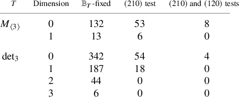
Remark 5.1. In the case of $M_{\langle 3\rangle }$
, all families either entirely passed or entirely failed each of the
$M_{\langle 3\rangle }$
, all families either entirely passed or entirely failed each of the $(210)$
and
$(210)$
and $(120)$
tests. In the case of
$(120)$
tests. In the case of $\operatorname {det}_3$
, some families split into a number of smaller-dimensional families upon application of the tests. Two of the four final candidates for
$\operatorname {det}_3$
, some families split into a number of smaller-dimensional families upon application of the tests. Two of the four final candidates for $\operatorname {det}_3$
started as isolated
$\operatorname {det}_3$
started as isolated ${\mathbb B}_T$
-fixed subspaces, and two are from one-dimensional families of
${\mathbb B}_T$
-fixed subspaces, and two are from one-dimensional families of ${\mathbb B}_T$
-fixed subspaces.
${\mathbb B}_T$
-fixed subspaces.
To avoid redundant work we make use of the observation that both $M_{\langle 3\rangle }$
and
$M_{\langle 3\rangle }$
and $\operatorname {det}_3$
are invariant under cyclic permutation of the factors, so once we have the
$\operatorname {det}_3$
are invariant under cyclic permutation of the factors, so once we have the $F_{110}$
candidates we automatically obtain the
$F_{110}$
candidates we automatically obtain the $F_{101}$
and
$F_{101}$
and $F_{011}$
candidates. For each triple of candidates, in these cases with no remaining parameters, one checks that the
$F_{011}$
candidates. For each triple of candidates, in these cases with no remaining parameters, one checks that the $(111)$
test is not passed, proving the theorems.
$(111)$
test is not passed, proving the theorems.
The module structure for matrix multiplication was discussed in §4. We now describe the relevant module structure for the determinant: Write $U,V=\mathbb C^m$
and
$U,V=\mathbb C^m$
and $A_1=\cdots =A_m=U{\mathord { \otimes } } V$
. The determinant
$A_1=\cdots =A_m=U{\mathord { \otimes } } V$
. The determinant $\operatorname {det}_m$
, considered as a tensor, spans the line
$\operatorname {det}_m$
, considered as a tensor, spans the line ${\Lambda ^{m}} U{\mathord { \otimes } } {\Lambda ^{m}} V\subset A_1{\mathord {\otimes \cdots \otimes } } A_m$
. Explicitly, letting
${\Lambda ^{m}} U{\mathord { \otimes } } {\Lambda ^{m}} V\subset A_1{\mathord {\otimes \cdots \otimes } } A_m$
. Explicitly, letting $A_{\alpha }$
have basis
$A_{\alpha }$
have basis $x^{\alpha }_{ij}$
,
$x^{\alpha }_{ij}$
,
 $$\begin{align*}\operatorname{det}_m=\sum_{\sigma,\tau\in {\mathfrak{S}}_m}\mathrm{{sgn}}(\sigma\tau) x^1_{\sigma(1)\tau(1)}{\mathord{\otimes\cdots\otimes}} x^m_{\sigma(m)\tau(m)}. \end{align*}$$
We will be concerned with the case $m=3$
, and we write
$m=3$
, and we write $A_1{\mathord { \otimes } } A_2{\mathord { \otimes } } A_3=A{\mathord { \otimes } } B{\mathord { \otimes } } C$
. As a tensor,
$A_1{\mathord { \otimes } } A_2{\mathord { \otimes } } A_3=A{\mathord { \otimes } } B{\mathord { \otimes } } C$
. As a tensor, $\operatorname {det}_3$
is invariant under
$\operatorname {det}_3$
is invariant under $(\operatorname {SL}(U)\times \operatorname {SL}(V))\rtimes \mathbb {Z}_2$
as well as
$(\operatorname {SL}(U)\times \operatorname {SL}(V))\rtimes \mathbb {Z}_2$
as well as $\mathfrak S_3$
. As an
$\mathfrak S_3$
. As an $\operatorname {SL}(U)\times \operatorname {SL}(V)$
-module,
$\operatorname {SL}(U)\times \operatorname {SL}(V)$
-module, $A{\mathord { \otimes } } B$
is
$A{\mathord { \otimes } } B$
is $U^{{\mathord { \otimes } } 2}{\mathord { \otimes } } V^{{\mathord { \otimes } } 2} =S^2U{\mathord { \otimes } } S^2V {\mathord {\,\oplus }\,} S^2U{\mathord { \otimes } } {\Lambda ^{2}} V{\mathord {\,\oplus }\,} {\Lambda ^{2}} U{\mathord { \otimes } } S^2 V {\mathord {\,\oplus }\,} {\Lambda ^{2}} U{\mathord { \otimes } } {\Lambda ^{2}} V$
, and
$U^{{\mathord { \otimes } } 2}{\mathord { \otimes } } V^{{\mathord { \otimes } } 2} =S^2U{\mathord { \otimes } } S^2V {\mathord {\,\oplus }\,} S^2U{\mathord { \otimes } } {\Lambda ^{2}} V{\mathord {\,\oplus }\,} {\Lambda ^{2}} U{\mathord { \otimes } } S^2 V {\mathord {\,\oplus }\,} {\Lambda ^{2}} U{\mathord { \otimes } } {\Lambda ^{2}} V$
, and $\operatorname {det}_3(C^*)={\Lambda ^{2}} U{\mathord { \otimes } } {\Lambda ^{2}} V$
. As
$\operatorname {det}_3(C^*)={\Lambda ^{2}} U{\mathord { \otimes } } {\Lambda ^{2}} V$
. As $\operatorname {SL}(U)\times \operatorname {SL}(V)$
-modules,
$\operatorname {SL}(U)\times \operatorname {SL}(V)$
-modules, $\operatorname {det}_3(C^*)^{\perp }$
is the dual of the complement to
$\operatorname {det}_3(C^*)^{\perp }$
is the dual of the complement to $\operatorname {det}_3(C^*)$
in
$\operatorname {det}_3(C^*)$
in $A{\mathord { \otimes } } B$
, and the weight diagram of
$A{\mathord { \otimes } } B$
, and the weight diagram of $A{\mathord { \otimes } } B$
is the tensor product of the diagram in Example 2.7 with the same diagram for
$A{\mathord { \otimes } } B$
is the tensor product of the diagram in Example 2.7 with the same diagram for $V{\mathord { \otimes } } V$
. Each of the three modules in the complement to
$V{\mathord { \otimes } } V$
. Each of the three modules in the complement to $\operatorname {det}_3(C^*)$
in
$\operatorname {det}_3(C^*)$
in $A{\mathord { \otimes } } B$
are multiplicity free, but there are weight multiplicities up to three, for example,
$A{\mathord { \otimes } } B$
are multiplicity free, but there are weight multiplicities up to three, for example, $ u_1u_2{\mathord { \otimes } } v_1v_2, u_1u_2{\mathord { \otimes } } v_1\wedge v_2$
, and
$ u_1u_2{\mathord { \otimes } } v_1v_2, u_1u_2{\mathord { \otimes } } v_1\wedge v_2$
, and $ u_1\wedge u_2{\mathord { \otimes } } v_1v_2 $
each have weight
$ u_1\wedge u_2{\mathord { \otimes } } v_1v_2 $
each have weight $(\omega _2^U|\omega _2^V)$
. Consequently, there are more and larger-dimensional
$(\omega _2^U|\omega _2^V)$
. Consequently, there are more and larger-dimensional ${\mathbb B}_T$
-fixed subspaces, as observed in the table above.
${\mathbb B}_T$
-fixed subspaces, as observed in the table above.
For the code and further discussion of the implementation details, see the supplemental materials at github.com/adconner/chlbapolar.
6 Representation theory relevant for matrix multiplication
Theorems 1.4 and 1.5(1),(2) may also be proved using computer calculations, but we present hand-checkable proofs to both illustrate the power of the method and lay groundwork for future results. This section establishes the representation theory needed for those proofs.
6.1 Refinement of the
$(210)$
test for matrix multiplication

Recall $A=U^*{\mathord { \otimes } } V$
,
$A=U^*{\mathord { \otimes } } V$
, $B=V^*{\mathord { \otimes } } W$
,
$B=V^*{\mathord { \otimes } } W$
, $C=W^*{\mathord { \otimes } } U$
and
$C=W^*{\mathord { \otimes } } U$
and $M_{\langle \mathbf {u},\mathbf {v},\mathbf {w}\rangle }=\operatorname {Id}_U{\mathord { \otimes } } \operatorname {Id}_V{\mathord { \otimes } } \operatorname {Id}_W$
and the notation
$M_{\langle \mathbf {u},\mathbf {v},\mathbf {w}\rangle }=\operatorname {Id}_U{\mathord { \otimes } } \operatorname {Id}_V{\mathord { \otimes } } \operatorname {Id}_W$
and the notation $\omega _j$
for the fundamental
$\omega _j$
for the fundamental $\mathfrak {sl}$
-weights from §2.5. Let
$\mathfrak {sl}$
-weights from §2.5. Let $V_{\mu }$
denote the irreducible
$V_{\mu }$
denote the irreducible $\mathfrak {sl}(V)$
-module with highest weight
$\mathfrak {sl}(V)$
-module with highest weight $\mu $
. We have the following decompositions as
$\mu $
. We have the following decompositions as $\operatorname {SL}(U)\times \operatorname {SL}(V)$
-modules: (note
$\operatorname {SL}(U)\times \operatorname {SL}(V)$
-modules: (note $V_{\omega _2+\omega _{\mathbf {v}-1}}$
does not appear when
$V_{\omega _2+\omega _{\mathbf {v}-1}}$
does not appear when $\mathbf {v}=2$
, and when
$\mathbf {v}=2$
, and when $\mathbf {v}=3$
,
$\mathbf {v}=3$
, $V_{\omega _2+\omega _{\mathbf {v}-1}}=V_{2\omega _2}$
):
$V_{\omega _2+\omega _{\mathbf {v}-1}}=V_{2\omega _2}$
):
 $$ \begin{align} {\Lambda^{2}} (U^*{\mathord{ \otimes } } V){\mathord{ \otimes } } V^*&= \begin{aligned}[t] &(S^2U^*{\mathord{ \otimes } } V_{\omega_1}){\mathord{\,\oplus }\,} ({\Lambda^{2}} U^*{\mathord{ \otimes } } V_{\omega_1}) \\ &{\mathord{\,\oplus }\,} (S^2U^*{\mathord{ \otimes } } V_{\omega_2+\omega_{\mathbf{v}-1}}){\mathord{\,\oplus }\,} ({\Lambda^{2}} U^*{\mathord{ \otimes } } V_{2\omega_1+\omega_{\mathbf{v}-1}}), \end{aligned} \end{align} $$
 $$ \begin{align} S^2(U^*{\mathord{ \otimes } } V){\mathord{ \otimes } } V^*&= \begin{aligned}[t] &(S^2U^*{\mathord{ \otimes } } V_{2\omega_1+\omega_{\mathbf{v}-1}}){\mathord{\,\oplus }\,} ({\Lambda^{2}} U^*{\mathord{ \otimes } } V_{\omega_2+\omega_{\mathbf{v}-1}}) \\ {}&{\mathord{\,\oplus }\,}(S^2U^*{\mathord{ \otimes } } V_{\omega_1}) {\mathord{\,\oplus }\,} ({\Lambda^{2}} U^*{\mathord{ \otimes } } V_{\omega_1} ), \end{aligned} \end{align} $$
 $$ \begin{align} A{\mathord{ \otimes } } M_{\langle \mathbf{u},\mathbf{v},\mathbf{w}\rangle}(C^*)&= \begin{aligned}[t] &(U^*{\mathord{ \otimes } } V){\mathord{ \otimes } } (U^*{\mathord{ \otimes } } \operatorname{Id}_V{\mathord{ \otimes } } W) \\ &= (S^2U^*{\mathord{ \otimes } } V_{\omega_1}{\mathord{ \otimes } } W){\mathord{\,\oplus }\,} ({\Lambda^{2}} U^*{\mathord{ \otimes } } V_{\omega_1} {\mathord{ \otimes } } W), \end{aligned} \end{align} $$
 $$ \begin{align} V{\mathord{ \otimes } } \mathfrak {sl}(V)&=V_{ \omega_1 }{\mathord{\,\oplus }\,} V_{2\omega_1+\omega_{\mathbf{v}-1}}{\mathord{\,\oplus }\,} V_{\omega_2+\omega_{\mathbf{v}-1}}, \end{align} $$
 $$ \begin{align} (U^*{\mathord{ \otimes } } V){\mathord{ \otimes } } (U^*{\mathord{ \otimes } } \mathfrak {sl}(V)) &= \begin{aligned}[t] &(S^2U^*{\mathord{ \otimes } } V_{2\omega_1+\omega_{\mathbf{v}-1}}){\mathord{\,\oplus }\,} ({\Lambda^{2}} U^*{\mathord{ \otimes } } V_{2\omega_1+\omega_{\mathbf{v}-1}}) \\ {}&{\mathord{\,\oplus }\,}(S^2U^*{\mathord{ \otimes } } V_{\omega_1} ) {\mathord{\,\oplus }\,} ({\Lambda^{2}} U^*{\mathord{ \otimes } } V_{\omega_1} ) \\ {}&{\mathord{\,\oplus }\,} (S^2U^*{\mathord{ \otimes } } V_{\omega_2+\omega_{\mathbf{v}-1}}) {\mathord{\,\oplus }\,} ({\Lambda^{2}} U^*{\mathord{ \otimes } } V_{\omega_2+\omega_{\mathbf{v}-1}}). \end{aligned} \end{align} $$
These formulas follow from the following basic formulas: for any vector spaces $U,V$
, one has the
$U,V$
, one has the $\operatorname {GL}(U)\times \operatorname {GL}(V)$
decompositions
$\operatorname {GL}(U)\times \operatorname {GL}(V)$
decompositions $S^2(U{\mathord { \otimes } } V)=S^2U{\mathord { \otimes } } S^2V{\mathord {\,\oplus }\,} {\Lambda ^{2}} U{\mathord { \otimes } } {\Lambda ^{2}} V$
; see, for example, [Reference Landsberg30, §2.7.1] and the decomposition
$S^2(U{\mathord { \otimes } } V)=S^2U{\mathord { \otimes } } S^2V{\mathord {\,\oplus }\,} {\Lambda ^{2}} U{\mathord { \otimes } } {\Lambda ^{2}} V$
; see, for example, [Reference Landsberg30, §2.7.1] and the decomposition ${\Lambda ^{2}} (U{\mathord { \otimes } } V)= S^2U{\mathord { \otimes } } {\Lambda ^{2}} V{\mathord {\,\oplus }\,} S^2 U{\mathord { \otimes } } {\Lambda ^{2}} V$
is derived similarly, and one has the
${\Lambda ^{2}} (U{\mathord { \otimes } } V)= S^2U{\mathord { \otimes } } {\Lambda ^{2}} V{\mathord {\,\oplus }\,} S^2 U{\mathord { \otimes } } {\Lambda ^{2}} V$
is derived similarly, and one has the $\operatorname {GL}(U)$
decomposition
$\operatorname {GL}(U)$
decomposition $U{\mathord { \otimes } } U=S^2U{\mathord {\,\oplus }\,} {\Lambda ^{2}} U$
. Finally, the Pieri formula (see, e.g., [Reference Fulton and Harris20, §6.1, eqns 6.8,6.9]) gives
$U{\mathord { \otimes } } U=S^2U{\mathord {\,\oplus }\,} {\Lambda ^{2}} U$
. Finally, the Pieri formula (see, e.g., [Reference Fulton and Harris20, §6.1, eqns 6.8,6.9]) gives $S^2V{\mathord { \otimes } } V^*=V_{2\omega _1}{\mathord { \otimes } } V_{\omega _{\mathbf {v}-1}}=V_{2\omega _1+ \omega _{\mathbf {v}-1}} {\mathord {\,\oplus }\,} V_{\omega _1}$
and
$S^2V{\mathord { \otimes } } V^*=V_{2\omega _1}{\mathord { \otimes } } V_{\omega _{\mathbf {v}-1}}=V_{2\omega _1+ \omega _{\mathbf {v}-1}} {\mathord {\,\oplus }\,} V_{\omega _1}$
and ${\Lambda ^{2}} V{\mathord { \otimes } } V^*=V_{\omega _2}{\mathord { \otimes } } V_{\omega _{\mathbf {v}-1}}=V_{\omega _2+\omega _{\mathbf {v}-1}}{\mathord {\,\oplus }\,} V_{\omega _1}$
.
${\Lambda ^{2}} V{\mathord { \otimes } } V^*=V_{\omega _2}{\mathord { \otimes } } V_{\omega _{\mathbf {v}-1}}=V_{\omega _2+\omega _{\mathbf {v}-1}}{\mathord {\,\oplus }\,} V_{\omega _1}$
.
Note that $V_{\omega _1}$
is isomorphic to V and
$V_{\omega _1}$
is isomorphic to V and
 $$\begin{align*}\textstyle \operatorname{dim}(V_{2\omega_1+\omega_{\mathbf{v}-1}}) = \frac {1}{2} \mathbf{v}^3+ \frac{1} {2} \mathbf{v}^2 -\mathbf{v} , \ \ \ \operatorname{dim}( V_{\omega_2+\omega_{\mathbf{v}-1}} )=\frac {1}{2}\mathbf{v}^3-\frac{1}{ 2}\mathbf{v}^2-\mathbf{v}. \end{align*}$$
Proposition 6.1. Write $E_{110}:=M_{\langle \mathbf {u},\mathbf {v},\mathbf {w}\rangle }(C^*){\mathord {\,\oplus }\,} E_{110}'$
, where
$E_{110}:=M_{\langle \mathbf {u},\mathbf {v},\mathbf {w}\rangle }(C^*){\mathord {\,\oplus }\,} E_{110}'$
, where $E_{110}'\subset U^*{\mathord { \otimes } } \mathfrak {sl}(V){\mathord { \otimes } } W$
. The dimension of the kernel of the map (7)
$E_{110}'\subset U^*{\mathord { \otimes } } \mathfrak {sl}(V){\mathord { \otimes } } W$
. The dimension of the kernel of the map (7) $E_{110}{\mathord { \otimes } } A {\mathord {\;\rightarrow \;}} {\Lambda ^{2}} A{\mathord { \otimes } } B$
equals the dimension of the kernel of the skew symmetrization followed by projection map
$E_{110}{\mathord { \otimes } } A {\mathord {\;\rightarrow \;}} {\Lambda ^{2}} A{\mathord { \otimes } } B$
equals the dimension of the kernel of the skew symmetrization followed by projection map
 $$ \begin{align} E_{110}'{\mathord{ \otimes } } A {\mathord{\;\rightarrow\;}} S^2U^*{\mathord{ \otimes } } V_{\omega_2+\omega_{\mathbf{v}-1}}{\mathord{ \otimes } } W{\mathord{\,\oplus }\,} {\Lambda^{2}} U^*{\mathord{ \otimes } } V_{2\omega_1+\omega_{\mathbf{v}-1}}{\mathord{ \otimes } } W, \end{align} $$
and the kernel of equation (14) is
 $$ \begin{align} (E_{110}'{\mathord{ \otimes } } A )\cap [ U^{*{\mathord{ \otimes } } 2}{\mathord{ \otimes } } V_{\omega_1}{\mathord{ \otimes } } W{\mathord{\,\oplus }\,} S^2U^*{\mathord{ \otimes } } V_{2\omega_1+\omega_{\mathbf{v}-1}}{\mathord{ \otimes } } W{\mathord{\,\oplus }\,} {\Lambda^{2}} U^*{\mathord{ \otimes } } V_{\omega_2+\omega_{\mathbf{v}-1}}{\mathord{ \otimes } } W]. \end{align} $$
Proof. Write M for the target of equation (14). We have the following commutative diagram, where horizontal arrows form exact sequences:

The bottom row reflects the decomposition (9) tensored with W. The middle vertical arrow is the skew symmetrization map (7), and since it is the restriction of a $\operatorname {GL}(U)\times \operatorname {GL}(V)\times \operatorname {GL}(W)$
equivariant map, by Schur’s lemma, its submodule
$\operatorname {GL}(U)\times \operatorname {GL}(V)\times \operatorname {GL}(W)$
equivariant map, by Schur’s lemma, its submodule $(U^*{\mathord { \otimes } } \operatorname {Id}_V{\mathord { \otimes } } W) {\mathord { \otimes } } A = (U^*{\mathord { \otimes } } V) {\mathord { \otimes } } (U^*{\mathord { \otimes } } \operatorname {Id}_V{\mathord { \otimes } } W)$
must have image contained in
$(U^*{\mathord { \otimes } } \operatorname {Id}_V{\mathord { \otimes } } W) {\mathord { \otimes } } A = (U^*{\mathord { \otimes } } V) {\mathord { \otimes } } (U^*{\mathord { \otimes } } \operatorname {Id}_V{\mathord { \otimes } } W)$
must have image contained in $(U^*)^{{\mathord { \otimes } } 2}{\mathord { \otimes } } V_{\omega _1}{\mathord { \otimes } } W$
. The induced right vertical arrow is the map (14).
$(U^*)^{{\mathord { \otimes } } 2}{\mathord { \otimes } } V_{\omega _1}{\mathord { \otimes } } W$
. The induced right vertical arrow is the map (14).
We show the left vertical arrow is an isomorphism, from which the claim on the kernel dimension of equation (14) will follow by, for example, the snake lemma. We have the decomposition into irreducible modules
 $$\begin{align*}(U^*{\mathord{ \otimes } } V){\mathord{ \otimes } } (U^*{\mathord{ \otimes } } \operatorname{Id}_V{\mathord{ \otimes } } W)=S^2U^*{\mathord{ \otimes } } V{\mathord{ \otimes } } \operatorname{Id}_V{\mathord{ \otimes } } W{\mathord{\,\oplus }\,} {\Lambda^{2}} U^*{\mathord{ \otimes } } V{\mathord{ \otimes } } \operatorname{Id}_V{\mathord{ \otimes } } W. \end{align*}$$
The vertical left arrow is an equivariant map, so by Schur’s lemma, it is sufficient to see that a single vector in each of the modules on the right has nonzero image. We check the highest weight vectors:
 $$ \begin{align*} &(u^{\mathbf{u}} {\mathord{ \otimes } } v_1){\mathord{ \otimes } } u^{\mathbf{u}}{\mathord{ \otimes } } (\sum_j v_j{\mathord{ \otimes } } v^j){\mathord{ \otimes } } w_1 \mapsto \sum_{\rho>1} (u^{\mathbf{u}}{\mathord{ \otimes } } v_1)\wedge (u^{\mathbf{u}}{\mathord{ \otimes } } v_{\rho}) {\mathord{ \otimes } } v^{\rho}{\mathord{ \otimes } } w_1, \ \mathrm{and} \\ & \begin{aligned}[t] \big[(u^{\mathbf{u}} {\mathord{ \otimes } } v_1){\mathord{ \otimes } } u^{\mathbf{u}-1} - {}&(u^{\mathbf{u}-1} {\mathord{ \otimes } } v_1){\mathord{ \otimes } } u^{\mathbf{u}}\big ] {\mathord{ \otimes } } (\sum_j v_j{\mathord{ \otimes } } v^j){\mathord{ \otimes } } w_1 \mapsto \\ &\sum_j \big[(u^{\mathbf{u}}{\mathord{ \otimes } } v_1)\wedge (u^{\mathbf{u}-1}{\mathord{ \otimes } } v_j) -(u^{\mathbf{u}-1}{\mathord{ \otimes } } v_1)\wedge (u^{\mathbf{u}}{\mathord{ \otimes } } v_j)\big]{\mathord{ \otimes } } v^j{\mathord{ \otimes } } w_1 \end{aligned} \end{align*} $$
Now, equation (14) is a restriction of the surjective equivariant map $ U^*{\mathord { \otimes } } \mathfrak {sl}(V) {\mathord { \otimes } } W {\mathord { \otimes } } A\to M$
. Comparing modules in the irreducible decompositions of the source and target in view of equation (13), we obtain that equation (15) is the kernel of equation (14).
$ U^*{\mathord { \otimes } } \mathfrak {sl}(V) {\mathord { \otimes } } W {\mathord { \otimes } } A\to M$
. Comparing modules in the irreducible decompositions of the source and target in view of equation (13), we obtain that equation (15) is the kernel of equation (14).
6.2
$ \underline {\mathbf {R}}(M_{\langle 2\rangle })>6$
revisited

In this case, the map (14) takes image in ${\Lambda ^{2}} U^*{\mathord { \otimes } } S^2V{\mathord { \otimes } } V^*{\mathord { \otimes } } W$
. We have the following images.
${\Lambda ^{2}} U^*{\mathord { \otimes } } S^2V{\mathord { \otimes } } V^*{\mathord { \otimes } } W$
. We have the following images.
For the highest weight vector $x^2_1{\mathord { \otimes } } y^2_1$
times the four basis vectors of A (with their
$x^2_1{\mathord { \otimes } } y^2_1$
times the four basis vectors of A (with their $\mathfrak {sl}(V)$
-weights in the second column), the image of equation (14) is spanned by
$\mathfrak {sl}(V)$
-weights in the second column), the image of equation (14) is spanned by
 $$ \begin{align*} x^1_1\wedge x^2_1{\mathord{ \otimes } } y^2_1 & \quad 3\omega_1\\ x^1_2\wedge x^2_1{\mathord{ \otimes } } y^2_1 & \quad \omega_1. \end{align*} $$
(Note, e.g., $x^2_2{\mathord { \otimes } } x^2_1{\mathord { \otimes } } y^2_1$
maps to zero under the skew-symmetrization map as
$x^2_2{\mathord { \otimes } } x^2_1{\mathord { \otimes } } y^2_1$
maps to zero under the skew-symmetrization map as $u^2{\mathord { \otimes } } u^2$
projects to zero in
$u^2{\mathord { \otimes } } u^2$
projects to zero in ${\Lambda ^{2}} U^*$
.) For
${\Lambda ^{2}} U^*$
.) For $A{\mathord { \otimes } } (x^2_1{\mathord { \otimes } } y^1_1-x^2_2{\mathord { \otimes } } y^2_1)$
(the lowering of
$A{\mathord { \otimes } } (x^2_1{\mathord { \otimes } } y^1_1-x^2_2{\mathord { \otimes } } y^2_1)$
(the lowering of $x^2_1{\mathord { \otimes } } y^2_1$
under
$x^2_1{\mathord { \otimes } } y^2_1$
under $\mathfrak {sl}(V)$
), the image is spanned by
$\mathfrak {sl}(V)$
), the image is spanned by
 $$ \begin{align*} x^1_1\wedge (x^2_1{\mathord{ \otimes } } y^1_1-x^2_2{\mathord{ \otimes } } y^2_1) & \quad \omega_1\\ x^1_2\wedge (x^2_1{\mathord{ \otimes } } y^1_1-x^2_2{\mathord{ \otimes } } y^2_1) & \quad {-\omega_1}. \end{align*} $$
Since W has nothing to do with the map, we don’t need to compute the image of, for example, $A{\mathord { \otimes } } x^2_1{\mathord { \otimes } } y^2_2$
to know its contribution to the kernel, as it must be the same dimension as that of
$A{\mathord { \otimes } } x^2_1{\mathord { \otimes } } y^2_2$
to know its contribution to the kernel, as it must be the same dimension as that of $A{\mathord { \otimes } } x^2_1{\mathord { \otimes } } y^2_1$
, just with a different W-weight.
$A{\mathord { \otimes } } x^2_1{\mathord { \otimes } } y^2_1$
, just with a different W-weight.
Were $\underline {\mathbf {R}}(M_{\langle 2\rangle })=6$
,
$\underline {\mathbf {R}}(M_{\langle 2\rangle })=6$
, $E_{110}'$
would have dimension two, spanned by the highest weight vector and one lowering of it, and in order to be a candidate, its image in
$E_{110}'$
would have dimension two, spanned by the highest weight vector and one lowering of it, and in order to be a candidate, its image in ${\Lambda ^{2}} U^*{\mathord { \otimes } } S^3V{\mathord { \otimes } } W$
would have to have dimension at most two. Taking
${\Lambda ^{2}} U^*{\mathord { \otimes } } S^3V{\mathord { \otimes } } W$
would have to have dimension at most two. Taking $E_{110}'=\langle x^2_1{\mathord { \otimes } } y^2_1, x^2_1{\mathord { \otimes } } y^1_1-x^2_2{\mathord { \otimes } } y^2_1\rangle $
, the image of equation (14) has dimension three. Taking
$E_{110}'=\langle x^2_1{\mathord { \otimes } } y^2_1, x^2_1{\mathord { \otimes } } y^1_1-x^2_2{\mathord { \otimes } } y^2_1\rangle $
, the image of equation (14) has dimension three. Taking $E_{110}'=\langle x^2_1{\mathord { \otimes } } y^2_1, x^2_1{\mathord { \otimes } } y^2_2\rangle $
, the image of equation (14) has dimension four. Finally, taking
$E_{110}'=\langle x^2_1{\mathord { \otimes } } y^2_1, x^2_1{\mathord { \otimes } } y^2_2\rangle $
, the image of equation (14) has dimension four. Finally, taking $E_{110}'=\langle x^1_1{\mathord { \otimes } } y^2_1, x^2_1{\mathord { \otimes } } y^2_1\rangle $
, by transpose symmetry (see §4), the image of the
$E_{110}'=\langle x^1_1{\mathord { \otimes } } y^2_1, x^2_1{\mathord { \otimes } } y^2_1\rangle $
, by transpose symmetry (see §4), the image of the $(120)$
-version of equation (14) must have dimension four and we conclude.
$(120)$
-version of equation (14) must have dimension four and we conclude.
7 Proofs of Theorems 1.5 and 1.6
7.1 Overview
To prove border rank lower bounds for a fixed tensor using border apolarity, one checks a list of candidates for components of a multigraded ideal. It is not immediate how to extend the technique to sequences of tensors in $\mathbf {n}$
. Even in good situations such as in Theorems 1.5 and 1.6 where there are large Borel subgroups, candidate components can still occur in positive-dimensional families, and there is an exponential growth in
$\mathbf {n}$
. Even in good situations such as in Theorems 1.5 and 1.6 where there are large Borel subgroups, candidate components can still occur in positive-dimensional families, and there is an exponential growth in $\mathbf {n}$
in the number of families to check. We overcome this problem by introducing several new ideas.
$\mathbf {n}$
in the number of families to check. We overcome this problem by introducing several new ideas.
We restrict attention to only the (110)-graded ideal component and the application of the dual form of the (120) and (210) tests of §3. For each given candidate component, we forget everything about it except for the dimensions of certain internal weight spaces. We then analyze the kernels of Proposition 3.5 as sums of “local” contributions from each internal weight space. As we consider only dimension information, we determine upper bounds on the contributions. At this point, there are still many discrete cases of possible choices of these internal dimensions to consider. We use techniques from convex optimization to show that the relevant kernel contributions for any choice is no better than a constant more than that of a small fixed number of choices. We call this step the “globalization”. These choices can then be completely analyzed as functions of $\mathbf {n}$
.
$\mathbf {n}$
.
7.2 Preliminaries
Recall that in these proofs $\mathbf {u}=\mathbf {w}=\mathbf {n}$
and
$\mathbf {u}=\mathbf {w}=\mathbf {n}$
and $\mathbf {v}$
is
$\mathbf {v}$
is $2$
or
$2$
or $3$
. Let
$3$
. Let $E_{110}' \subset U^* {\mathord { \otimes } } \mathfrak {sl}(V) {\mathord { \otimes } } W$
be a
$E_{110}' \subset U^* {\mathord { \otimes } } \mathfrak {sl}(V) {\mathord { \otimes } } W$
be a ${\mathbb B}$
-fixed subspace. In particular,
${\mathbb B}$
-fixed subspace. In particular, $E_{110}'$
is fixed under the torus of
$E_{110}'$
is fixed under the torus of $\operatorname {GL}(U)\times \operatorname {GL}(W)$
, so we may write
$\operatorname {GL}(U)\times \operatorname {GL}(W)$
, so we may write $E_{110}' = \bigoplus _{s,t} u^{\mathbf {n}-s+1}{\mathord { \otimes } } X_{s,t} {\mathord { \otimes } } w_t$
, where
$E_{110}' = \bigoplus _{s,t} u^{\mathbf {n}-s+1}{\mathord { \otimes } } X_{s,t} {\mathord { \otimes } } w_t$
, where $X_{s,t}\subset \mathfrak {sl}(V)$
. Since
$X_{s,t}\subset \mathfrak {sl}(V)$
. Since $E_{110}'$
is fixed under the Borel subgroups of
$E_{110}'$
is fixed under the Borel subgroups of $\operatorname {GL}(U)$
,
$\operatorname {GL}(U)$
, $\operatorname {GL}(V)$
and
$\operatorname {GL}(V)$
and $\operatorname {GL}(W)$
, for each s and t we have
$\operatorname {GL}(W)$
, for each s and t we have
-
1.
$X_{s,t}\subset \mathfrak {sl}(V)$
is
${\mathbb B}_V\subset \operatorname {GL}(V)$
fixed, -
2.
$X_{s,t} \supset X_{s+1,t}$
and -
3.
$X_{s,t}\supset X_{s,t+1}$
.


Define the outer structure of $E_{110}'$
to be the data
$E_{110}'$
to be the data
 $$ \begin{align*}(s,t,\operatorname{dim} X_{s,t}), \ \ 0\leq s,t\leq\mathbf{n}. \end{align*} $$
Define the inner structure at site $(s,t)$
to be
$(s,t)$
to be $X_{s,t}$
.
$X_{s,t}$
.
We may consider the outer structure of $E_{110}'$
as an
$E_{110}'$
as an $\mathbf {n}\times \mathbf {n}$
grid, with each grid point
$\mathbf {n}\times \mathbf {n}$
grid, with each grid point $(s,t)$
labelled by the dimension of the corresponding
$(s,t)$
labelled by the dimension of the corresponding $X_{s,t}$
. We will represent such filled grids by the corresponding Young diagrams on the nonzero labels so that the upper left box corresponds with the highest weight. Here, labels weakly decrease going to the right and down. It is reasonable to imagine such a filled Young diagram rotated
$X_{s,t}$
. We will represent such filled grids by the corresponding Young diagrams on the nonzero labels so that the upper left box corresponds with the highest weight. Here, labels weakly decrease going to the right and down. It is reasonable to imagine such a filled Young diagram rotated $45^{\circ }$
clockwise to put the highest weight at the top, as in the corresponding weight diagram (see Example 2.9, where
$45^{\circ }$
clockwise to put the highest weight at the top, as in the corresponding weight diagram (see Example 2.9, where $\mathbf {n}=\mathbf {v}=2$
).
$\mathbf {n}=\mathbf {v}=2$
).
In the case of $\mathfrak {sl}_2$
, each
$\mathfrak {sl}_2$
, each $X_{s,t}$
is determined by its dimension, so an outer structure completely specifies a corresponding
$X_{s,t}$
is determined by its dimension, so an outer structure completely specifies a corresponding $E_{110}'$
. In the case of
$E_{110}'$
. In the case of $\mathfrak {sl}_3$
, information about the particular inner structures is lost passing from
$\mathfrak {sl}_3$
, information about the particular inner structures is lost passing from $E_{110}'$
to its outer structure.
$E_{110}'$
to its outer structure.
Example 7.1. Here are three examples with $\mathbf {v}=2$
and
$\mathbf {v}=2$
and $\rho =4$
.
$\rho =4$
.
The diagram
![]() corresponds to
corresponds to
 $$\begin{align*}E_{110}' = \langle u^{\mathbf{n}}{\mathord{ \otimes } } v^2{\mathord{ \otimes } } v_1{\mathord{ \otimes } } w_1, u^{\mathbf{n}}{\mathord{ \otimes } } v^2{\mathord{ \otimes } } v_1{\mathord{ \otimes } } w_2, u^{\mathbf{n}}{\mathord{ \otimes } } v^2{\mathord{ \otimes } } v_1{\mathord{ \otimes } } w_3, u^{\mathbf{n}-1}{\mathord{ \otimes } } v^2{\mathord{ \otimes } } v_1{\mathord{ \otimes } } w_1\rangle. \end{align*}$$
The diagram
![]() corresponds to
corresponds to
 $$\begin{align*}E_{110}' = \langle u^{\mathbf{n}}{\mathord{ \otimes } } v^2{\mathord{ \otimes } } v_1{\mathord{ \otimes } } w_1, u^{\mathbf{n}}{\mathord{ \otimes } } (v^1{\mathord{ \otimes } } v_1-v^2{\mathord{ \otimes } } v_2){\mathord{ \otimes } } w_1, u^{\mathbf{n}}{\mathord{ \otimes } } v^2{\mathord{ \otimes } } v_1{\mathord{ \otimes } } w_2, u^{\mathbf{n}-1}{\mathord{ \otimes } } v^2{\mathord{ \otimes } } v_1{\mathord{ \otimes } } w_1\rangle. \end{align*}$$
The diagram
![]() corresponds to
corresponds to
 $$\begin{align*}E_{110}' = \langle u^{\mathbf{n}}{\mathord{ \otimes } } v^2{\mathord{ \otimes } } v_1{\mathord{ \otimes } } w_1, u^{\mathbf{n}}{\mathord{ \otimes } } (v^1{\mathord{ \otimes } } v_1-v^2{\mathord{ \otimes } } v_2){\mathord{ \otimes } } w_1, u^{\mathbf{n}}{\mathord{ \otimes } } v^1{\mathord{ \otimes } } v_2{\mathord{ \otimes } } w_1, u^{\mathbf{n}}{\mathord{ \otimes } } v^2{\mathord{ \otimes } } v_1{\mathord{ \otimes } } w_2\rangle. \end{align*}$$
The transpose symmetry discussed in §4 maps $ E_{110}' = \bigoplus _{s,t} u^{\mathbf {n}-s+1}{\mathord { \otimes } } X_{s,t} {\mathord { \otimes } } w_t$
to
$ E_{110}' = \bigoplus _{s,t} u^{\mathbf {n}-s+1}{\mathord { \otimes } } X_{s,t} {\mathord { \otimes } } w_t$
to $\bigoplus _{s,t} u^{\mathbf {n}-t+1}{\mathord { \otimes } } X_{s,t}^{\mathbf {t}} {\mathord { \otimes } } w_s$
, that is, the inner structure at site
$\bigoplus _{s,t} u^{\mathbf {n}-t+1}{\mathord { \otimes } } X_{s,t}^{\mathbf {t}} {\mathord { \otimes } } w_s$
, that is, the inner structure at site $(s,t)$
becomes the transpose of the inner structure at site
$(s,t)$
becomes the transpose of the inner structure at site $(t,s)$
. In particular, transpose symmetry conjugates the diagram corresponding to the outer structure. In view of this symmetry, it is sufficient to study the
$(t,s)$
. In particular, transpose symmetry conjugates the diagram corresponding to the outer structure. In view of this symmetry, it is sufficient to study the $(210)$
test only, for then everything we can say is also a statement about the
$(210)$
test only, for then everything we can say is also a statement about the $(120)$
test under this transpose.
$(120)$
test under this transpose.
As mentioned above, we split the calculation of the kernel into a local and global computation. We bound the local contribution to the kernel at site $(s,t)$
by a function of
$(s,t)$
by a function of $s,t$
and
$s,t$
and $\operatorname {dim} X_{s,t}$
. Once this is done, the theorems are proved by solving the resulting combinatorial optimization problem over outer structures.
$\operatorname {dim} X_{s,t}$
. Once this is done, the theorems are proved by solving the resulting combinatorial optimization problem over outer structures.
Recall the expression (15) and let K denote the term in brackets, that is,
 $$ \begin{align} \begin{aligned} K &= (U^*)^{{\mathord{ \otimes } } 2}{\mathord{ \otimes } } V_{\omega_1}{\mathord{ \otimes } } W{\mathord{\,\oplus }\,} S^2U^* {\mathord{ \otimes } } V_{2\omega_1+\omega_{\mathbf{v}-1}}{\mathord{ \otimes } } W{\mathord{\,\oplus }\,} {\Lambda^{2}} U^*{\mathord{ \otimes } } V_{\omega_2+\omega_{\mathbf{v}-1}}{\mathord{ \otimes } } W \\ &\subset (U^*)^{{\mathord{ \otimes } } 2} {\mathord{ \otimes } } V{\mathord{ \otimes } } \mathfrak {sl}(V) {\mathord{ \otimes } } W. \end{aligned} \end{align} $$
We may filter $E_{110}'$
by
$E_{110}'$
by ${\mathbb B}$
-fixed subspaces such that each quotient corresponds to the inner structure contribution over some site
${\mathbb B}$
-fixed subspaces such that each quotient corresponds to the inner structure contribution over some site $(s,t)$
. Call such a filtration admissible. Let
$(s,t)$
. Call such a filtration admissible. Let $\Sigma _1\subset \Sigma _2\subset \cdots \subset \Sigma _f= E_{110}'$
be an admissible filtration, and put
$\Sigma _1\subset \Sigma _2\subset \cdots \subset \Sigma _f= E_{110}'$
be an admissible filtration, and put
 $$ \begin{align} K_g = (\Sigma_g {\mathord{ \otimes } } A )\cap K. \end{align} $$
Then the dimension of equation (15) may be written as the sum over g of $ \mathrm {dim}\; (K_g/K_{g-1})$
, and we may upper bound the dimension of equation (15) by upper bounding each
$ \mathrm {dim}\; (K_g/K_{g-1})$
, and we may upper bound the dimension of equation (15) by upper bounding each $\mathrm {dim}\; (K_g/K_{g-1})$
. We obtain bounds on
$\mathrm {dim}\; (K_g/K_{g-1})$
. We obtain bounds on $\mathrm {dim}\; (K_g/K_{g-1})$
which depend only on s and
$\mathrm {dim}\; (K_g/K_{g-1})$
which depend only on s and $j=j_g := \mathrm {dim}\; (\Sigma _g / \Sigma _{g-1})$
. For
$j=j_g := \mathrm {dim}\; (\Sigma _g / \Sigma _{g-1})$
. For $\mathfrak {sl}_2$
, this is Lemma 7.2, and for
$\mathfrak {sl}_2$
, this is Lemma 7.2, and for $\mathfrak {sl}_3$
, this is Lemma 7.4. As discussed above, bounds on the kernel of the
$\mathfrak {sl}_3$
, this is Lemma 7.4. As discussed above, bounds on the kernel of the $(120)$
map are obtained by symmetry; specifically, the bound is the same with s replaced by t.
$(120)$
map are obtained by symmetry; specifically, the bound is the same with s replaced by t.
Once these lemmas are established, the claims on fixed finite values of $\mathbf {n}$
may be immediately settled by enumerating the finitely many possible outer structures and checking that none gives a large enough kernel for both the
$\mathbf {n}$
may be immediately settled by enumerating the finitely many possible outer structures and checking that none gives a large enough kernel for both the $(210)$
and
$(210)$
and $(120)$
maps. The claims on infinite sequences of
$(120)$
maps. The claims on infinite sequences of $\mathbf {n}$
require us to work more carefully, and we prove the required bounds on the solution to such problems parameterized by
$\mathbf {n}$
require us to work more carefully, and we prove the required bounds on the solution to such problems parameterized by $\mathbf {n}$
in Lemma 7.7.
$\mathbf {n}$
in Lemma 7.7.
7.3 The local argument
Lemma 7.2. Let $\operatorname {dim} V=2$
,
$\operatorname {dim} V=2$
, $\operatorname {dim} U=\mathbf {n}$
. Fix an admissible filtration such that
$\operatorname {dim} U=\mathbf {n}$
. Fix an admissible filtration such that $ \Sigma _g\subset E_{110}'$
contains the
$ \Sigma _g\subset E_{110}'$
contains the $\mathfrak {sl}(V)$
-subspace at site
$\mathfrak {sl}(V)$
-subspace at site $(s,t)$
and
$(s,t)$
and $\Sigma _{g-1}$
does not. Write j for the dimension of the
$\Sigma _{g-1}$
does not. Write j for the dimension of the $\mathfrak {sl}(V)$
-subspace at site
$\mathfrak {sl}(V)$
-subspace at site $(s,t)$
. Then
$(s,t)$
. Then
 $$ \begin{align*}\operatorname{dim} (K_g/ K_{g-1})=a_js+b_j, \end{align*} $$
where $a_j,b_j$
are the following functions of j:
$a_j,b_j$
are the following functions of j:

Lemma 7.2 is proved later this section.
Remark 7.3. Revisiting the proof that $\underline {\mathbf {R}}(M_{\langle 2\rangle })>6$
in this language, the possible outer structures of
$\underline {\mathbf {R}}(M_{\langle 2\rangle })>6$
in this language, the possible outer structures of ${\mathbb B}$
-fixed two planes are
${\mathbb B}$
-fixed two planes are
![]() ,
,
![]() ,
,
![]() , which, according to Lemma 7.2, have
, which, according to Lemma 7.2, have $(210)$
map kernel dimensions
$(210)$
map kernel dimensions $5=3(1)+2$
,
$5=3(1)+2$
, $6=(1(2)+0)+(2(2)+0)$
, and
$6=(1(2)+0)+(2(2)+0)$
, and $4= (1(2)+0)+(1(2)+0)$
, respectively. The first and third are smaller than
$4= (1(2)+0)+(1(2)+0)$
, respectively. The first and third are smaller than $6$
and the choice of
$6$
and the choice of
![]() fails the
fails the $(120)$
test by transpose symmetry. This gives our shortest proof that
$(120)$
test by transpose symmetry. This gives our shortest proof that $\underline {\mathbf {R}}(M_{\langle 2\rangle })>6$
.
$\underline {\mathbf {R}}(M_{\langle 2\rangle })>6$
.
Proof of Theorem 1.4.
Here, we take $\mathbf {u}=2$
,
$\mathbf {u}=2$
, $\mathbf {w}= 3$
,
$\mathbf {w}= 3$
, $\mathbf {v}=2$
. We show that there is no
$\mathbf {v}=2$
. We show that there is no $E_{110}'$
of dimension
$E_{110}'$
of dimension $3=9-6$
passing the
$3=9-6$
passing the $(210)$
and
$(210)$
and $(120)$
tests. The possible outer structures are
$(120)$
tests. The possible outer structures are
![]() ,
,
![]() ,
,
![]() and
and
![]() . Applying Lemma 7.2 with
. Applying Lemma 7.2 with $\mathbf {n}=2$
, the corresponding
$\mathbf {n}=2$
, the corresponding $(210)$
map kernel dimensions are eight, seven, six and nine, respectively, so only
$(210)$
map kernel dimensions are eight, seven, six and nine, respectively, so only
![]() passes. However,
passes. However,
![]() has
has $(120)$
kernel dimension eight and fails this test.
$(120)$
kernel dimension eight and fails this test.
Proof of Theorem 1.5(1),(2).
For Theorem 1.5(1), $\mathbf {u}=\mathbf {w}=3$
,
$\mathbf {u}=\mathbf {w}=3$
, $\mathbf {v}=2$
. The outer structures corresponding to
$\mathbf {v}=2$
. The outer structures corresponding to $13-9=4$
dimensional subpaces of
$13-9=4$
dimensional subpaces of $U^*{\mathord { \otimes } } \mathfrak {sl}(V){\mathord { \otimes } } W$
are
$U^*{\mathord { \otimes } } \mathfrak {sl}(V){\mathord { \otimes } } W$
are
![]() ,
,
![]() ,
,
![]() ,
,
![]() ,
,
![]() ,
,
![]() ,
,
![]() ,
,
![]() ,
,
![]() ,
,
![]() . Of these,
. Of these,
![]() ,
,
![]() ,
,
![]() , and
, and
![]() pass the
pass the $(210)$
test with kernel dimensions of size
$(210)$
test with kernel dimensions of size $14$
,
$14$
, $16$
,
$16$
, $15$
, and
$15$
, and $14$
, respectively. However, none of these pass the
$14$
, respectively. However, none of these pass the $(120)$
test as none appear in this list whose conjugate tableau also appear.
$(120)$
test as none appear in this list whose conjugate tableau also appear.
For Theorem 1.5(2), the result follows by similar complete enumeration of outer structures on a computer.
Lemma 7.4. Let $\operatorname {dim} V=3$
,
$\operatorname {dim} V=3$
, $\operatorname {dim} U=\mathbf {n}$
. Fix an admissible filtration such that
$\operatorname {dim} U=\mathbf {n}$
. Fix an admissible filtration such that $ \Sigma _g\subset E_{110}'$
contains the
$ \Sigma _g\subset E_{110}'$
contains the $\mathfrak {sl}(V)$
-subspace at site
$\mathfrak {sl}(V)$
-subspace at site $(s,t)$
and
$(s,t)$
and $\Sigma _{g-1}$
does not. Write j for the dimension of the
$\Sigma _{g-1}$
does not. Write j for the dimension of the $\mathfrak {sl}(V)$
-subspace at site
$\mathfrak {sl}(V)$
-subspace at site $(s,t)$
. Then
$(s,t)$
. Then
 $$ \begin{align*}\operatorname{dim} (K_g/ K_{g-1})\leq a_js+b_j, \end{align*} $$
where $a_j,b_j$
are the following functions of j:
$a_j,b_j$
are the following functions of j:

In order to prove Lemmas 7.2 and 7.4, we first observe the following.
Proposition 7.5. The included module $V_{\omega _1} \subset V{\mathord { \otimes } } \mathfrak {sl}(V)$
has weight basis
$V_{\omega _1} \subset V{\mathord { \otimes } } \mathfrak {sl}(V)$
has weight basis
 $$ \begin{align*}\overline{v}_i := \sum_{j\neq i} [\mathbf{v} v_j{\mathord{ \otimes } } (v_i{\mathord{ \otimes } } v^j)- v_i{\mathord{ \otimes } } (v_j{\mathord{ \otimes } } v^j)] + (\mathbf{v}-1) v_i{\mathord{ \otimes } } v_i{\mathord{ \otimes } } v^i, \ \ 1\leq i\leq \mathbf{v}. \end{align*} $$
Proof. The line $[\overline {v}_1]$
has weight
$[\overline {v}_1]$
has weight $\omega _1=\epsilon _1$
and is
$\omega _1=\epsilon _1$
and is ${\mathbb B}$
-stable, the lines
${\mathbb B}$
-stable, the lines $[\overline {v}_i]$
are lowerings of the line
$[\overline {v}_i]$
are lowerings of the line $[\overline {v}_1]$
and have weight
$[\overline {v}_1]$
and have weight $\epsilon _i$
.
$\epsilon _i$
.
Proof of Lemmas 7.2 and 7.4.
We begin in somewhat greater generality, not fixing $\mathbf {v}=\operatorname {dim} V$
. We must bound
$\mathbf {v}=\operatorname {dim} V$
. We must bound $\mathrm {dim}\; K_g - \mathrm {dim}\; K_{g-1}$
, where
$\mathrm {dim}\; K_g - \mathrm {dim}\; K_{g-1}$
, where $K_g$
is given by equation (17). Write
$K_g$
is given by equation (17). Write $X\subset \mathfrak {sl}(V)$
for the inner structure at
$X\subset \mathfrak {sl}(V)$
for the inner structure at $(s,t)$
so that
$(s,t)$
so that $\Sigma _g=\Sigma _{g-1} \oplus u^{\mathbf {n}-s+1} {\mathord { \otimes } } X {\mathord { \otimes } } w_t$
. Write
$\Sigma _g=\Sigma _{g-1} \oplus u^{\mathbf {n}-s+1} {\mathord { \otimes } } X {\mathord { \otimes } } w_t$
. Write
 $$ \begin{align*}V_0 &= \varnothing,\\ V_1 &= V_{\omega_1}, \\ V_2& = V_{\omega_1} {\mathord{\,\oplus }\,} V_{2\omega_1+\omega_{\mathbf{v}-1}}, \\ V_3 &= V_{\omega_1} {\mathord{\,\oplus }\,} V_{2\omega_1+\omega_{\mathbf{v}-1}} {\mathord{\,\oplus }\,} V_{\omega_2+\omega_{\mathbf{v}-1}} = V{\mathord{ \otimes } } \mathfrak {sl}(V). \end{align*} $$
Note that $V_2 = V_3$
when
$V_2 = V_3$
when $\mathbf {v} = 2$
. Then
$\mathbf {v} = 2$
. Then $\{V_f\}_f$
is a (partial) flag for
$\{V_f\}_f$
is a (partial) flag for $V{\mathord { \otimes } } \mathfrak {sl}(V)$
, and
$V{\mathord { \otimes } } \mathfrak {sl}(V)$
, and
 $$ \begin{align*} S_f := U^*{\mathord{ \otimes } } U^{*(s-1)}{\mathord{ \otimes } } V_3 {\mathord{ \otimes } } W + U^{*{\mathord{ \otimes } } 2} {\mathord{ \otimes } } V_f {\mathord{ \otimes } } W + U^{*{\mathord{ \otimes } } 2}{\mathord{ \otimes } } V_3 {\mathord{ \otimes } } W_{(t-1)} \end{align*} $$
is a flag for $U^{*{\mathord { \otimes } } 2}{\mathord { \otimes } } V_3{\mathord { \otimes } } W$
, where we have written
$U^{*{\mathord { \otimes } } 2}{\mathord { \otimes } } V_3{\mathord { \otimes } } W$
, where we have written $U^{*(s)} = \mathrm {span}\{u^{\mathbf {n}},\ldots ,u^{\mathbf {n}-s+1}\}$
and
$U^{*(s)} = \mathrm {span}\{u^{\mathbf {n}},\ldots ,u^{\mathbf {n}-s+1}\}$
and $W_{(t )} = \mathrm {span}\{w_1,\ldots , w_t\}$
. Hence,
$W_{(t )} = \mathrm {span}\{w_1,\ldots , w_t\}$
. Hence, $S_f\cap K_g$
is a flag for
$S_f\cap K_g$
is a flag for $K_g$
with
$K_g$
with $S_3\cap K_g = K_g$
and
$S_3\cap K_g = K_g$
and $S_0\cap K_g \subseteq K_{g-1}$
. The fact that the inclusion
$S_0\cap K_g \subseteq K_{g-1}$
. The fact that the inclusion $S_0\cap K_g\subseteq K_{g-1}$
may be strict is the only place in this argument we prove an inequality rather than equality. Use the isomorphism of quotient vector spaces
$S_0\cap K_g\subseteq K_{g-1}$
may be strict is the only place in this argument we prove an inequality rather than equality. Use the isomorphism of quotient vector spaces
 $$ \begin{align} \frac{K_g\cap S_f}{K_g\cap S_{f-1}} = \frac{(K_g\cap S_f) + S_{f-1}}{S_{f-1}} \end{align} $$
to obtain the successive quotients of $\{S_f \cap K_g\}_f$
as subspaces of
$\{S_f \cap K_g\}_f$
as subspaces of
 $$ \begin{align} \frac{U^{*{\mathord{ \otimes } } 2}{\mathord{ \otimes } } V_3{\mathord{ \otimes } } W }{ S_{f-1}}=\frac{U^{*{\mathord{ \otimes } } 2}} { U^*{\mathord{ \otimes } } U^{*(s-1)}} \otimes \frac{V_3}{V_{f-1}} \otimes \frac{W}{W_{(t-1)} }. \end{align} $$
Write $K^f$
for the f-th summand of equation (16) so that
$K^f$
for the f-th summand of equation (16) so that $K \cap S_f = K^f + K\cap S_{f-1}$
. Intersecting with
$K \cap S_f = K^f + K\cap S_{f-1}$
. Intersecting with $\Sigma _g{\mathord { \otimes } } A$
and adding
$\Sigma _g{\mathord { \otimes } } A$
and adding $S_{f-1}$
, we obtain
$S_{f-1}$
, we obtain
 $$ \begin{align*}K_g\cap S_f + S_{f-1} &= (K^f + S_{f-1}) \cap (\Sigma_g {\mathord{ \otimes } } A) + S_{f-1}\\ & = (K^f + S_{f-1}) \cap (U^*{\mathord{ \otimes } } u^{\mathbf{n}-s+1}{\mathord{ \otimes } } V{\mathord{ \otimes } } X {\mathord{ \otimes } } w_t + S_{f-1}). \end{align*} $$
We may now pass in each side of the intersection to the right-hand side of equation (19), after which the intersection may be computed term by term. To compute the intersection in the $U^{*{\mathord { \otimes } } 2} /(U^*{\mathord { \otimes } } U^{*(s-1)})$
term, momentarily write
$U^{*{\mathord { \otimes } } 2} /(U^*{\mathord { \otimes } } U^{*(s-1)})$
term, momentarily write $\overline {Z} = Z + U^*{\mathord { \otimes } } U^{*(s-1)}$
for
$\overline {Z} = Z + U^*{\mathord { \otimes } } U^{*(s-1)}$
for $Z\in U^{*{\mathord { \otimes } } 2}$
and observe that
$Z\in U^{*{\mathord { \otimes } } 2}$
and observe that
 $$ \begin{align*}\overline{S^2 U^*} \cap \overline{ U^*{\mathord{ \otimes } } u^{\mathbf{n}-s+1}} = \overline{U^{*s} {\mathord{ \otimes } } u^{\mathbf{n}-s+1}}, \ \mathrm{and} \ \overline{{\Lambda^{2}} U^*} \cap \overline{U^*{\mathord{ \otimes } } u^{\mathbf{n}-s+1}} = \overline{U^{*(s-1)} {\mathord{ \otimes } } u^{\mathbf{n}-s+1}}. \end{align*} $$
Therefore, the right-hand side of equation (18) may be written, for $f=1$
,
$f=1$
, $2$
and
$2$
and $3$
respectively,
$3$
respectively,
 $$ \begin{gather*} U^*\otimes (u^{\mathbf{n}-s+1} + U^{*(s-1)}) \otimes [(V\otimes X)\cap V_1 ]\otimes (w_t + W_{(t-1)})\\ U^{*s}\otimes (u^{\mathbf{n}-s+1} + U^{*(s-1)}) \otimes [(V\otimes X + V_1) \cap V_2 ]\otimes (w_t + W_{(t-1)})\\ U^{*(s-1)}\otimes (u^{\mathbf{n}-s+1} + U^{*(s-1)}) \otimes [V\otimes X + V_2 ]\otimes (w_t + W_{(t-1)}). \end{gather*} $$
Write
 $$ \begin{align*}Y &= (V{\mathord{ \otimes } } X)\cap V_1,\\ Y' &= ((V{\mathord{ \otimes } } X + V_1)\cap V_2)/ V_1, \mathrm{\ and }\\ Y" &= (V{\mathord{ \otimes } } X + V_2)/ V_2, \end{align*} $$
and write their dimensions, respectively, as $\mathbf {y},\mathbf {y}',\mathbf {y}"$
. We obtain
$\mathbf {y},\mathbf {y}',\mathbf {y}"$
. We obtain
 $$ \begin{align*}\mathrm{dim}\; K_g =\mathrm{dim}\; (S_0\cap K_g) + \mathbf{y}\mathbf{n} + \mathbf{y}'s + \mathbf{y}"(s-1)\leq \mathrm{dim}\; K_{g-1} + \mathbf{y}\mathbf{n} + \mathbf{y}'s + \mathbf{y}"(s-1), \end{align*} $$
the sum of the successive quotient dimensions of $\{S_f\cap K_g\}_f$
.
$\{S_f\cap K_g\}_f$
.
Thus, when $j=\mathbf {v}^2 - 1$
, that is,
$j=\mathbf {v}^2 - 1$
, that is, $X=\mathfrak {sl}(V)$
, the desired result follows from
$X=\mathfrak {sl}(V)$
, the desired result follows from $\mathbf {y} = \mathbf {v}$
,
$\mathbf {y} = \mathbf {v}$
, $\mathbf {y}' = \mathrm {dim}\; V_{2\omega _{1}+\omega _{\mathbf {v}-1}}$
and
$\mathbf {y}' = \mathrm {dim}\; V_{2\omega _{1}+\omega _{\mathbf {v}-1}}$
and $\mathbf {y}" = \mathrm {dim}\; V_{\omega _{2}+\omega _{\mathbf {v}-1}}$
.
$\mathbf {y}" = \mathrm {dim}\; V_{\omega _{2}+\omega _{\mathbf {v}-1}}$
.
In all cases, Y has a basis consisting of weight vectors and is closed under raising operators. Hence, by Proposition 7.5, $Y = \mathrm {span} \{\overline {v}_i\mid i\le \mathbf {y} \}$
.
$Y = \mathrm {span} \{\overline {v}_i\mid i\le \mathbf {y} \}$
.
Consider the case $j=\mathbf {v}^2-2$
, that is X is the span of all weight vectors of
$j=\mathbf {v}^2-2$
, that is X is the span of all weight vectors of $\mathfrak {sl}(V)$
except
$\mathfrak {sl}(V)$
except $v_{\mathbf {v}} {\mathord { \otimes } } v^1$
. Then
$v_{\mathbf {v}} {\mathord { \otimes } } v^1$
. Then $\overline {v}_{\mathbf {v}}$
is not an element of Y because in the monomial basis, the monomial
$\overline {v}_{\mathbf {v}}$
is not an element of Y because in the monomial basis, the monomial $v_1{\mathord { \otimes } } (v_{\mathbf {v}}{\mathord { \otimes } } v^1)$
fails to have a nonzero coefficient in any element of Y. Hence,
$v_1{\mathord { \otimes } } (v_{\mathbf {v}}{\mathord { \otimes } } v^1)$
fails to have a nonzero coefficient in any element of Y. Hence, $\mathbf {y} \le \mathbf {v} -1$
, and the trivial
$\mathbf {y} \le \mathbf {v} -1$
, and the trivial $\mathbf {y}' \le \mathrm {dim}\; V_{2\omega _{1}+\omega _{\mathbf {v}-1}}$
, and
$\mathbf {y}' \le \mathrm {dim}\; V_{2\omega _{1}+\omega _{\mathbf {v}-1}}$
, and $\mathbf {y}" \le \mathrm {dim}\; V_{\omega _{2}+\omega _{\mathbf {v}-1}}$
give the asserted upper bounds.
$\mathbf {y}" \le \mathrm {dim}\; V_{\omega _{2}+\omega _{\mathbf {v}-1}}$
give the asserted upper bounds.
By similar reasoning, when $\mathbf {v} =3$
, considering Example 2.6, we obtain the bounds
$\mathbf {v} =3$
, considering Example 2.6, we obtain the bounds $\mathbf {y} = 0$
when
$\mathbf {y} = 0$
when $j=1,2$
and
$j=1,2$
and $\mathbf {y} \le 1$
when
$\mathbf {y} \le 1$
when $j=3,4,5,6$
. For all values of j except
$j=3,4,5,6$
. For all values of j except $1$
, the result then follows from
$1$
, the result then follows from
 $$ \begin{align} \mathrm{dim}\; K_g - \mathrm{dim}\; K_{g-1} &\leq (j\mathbf{v} - \mathbf{y})s + \mathbf{y} \mathbf{n} - \mathbf{y}"\\ &\nonumber \le (j\mathbf{v} - \mathbf{y})s + \mathbf{y}\mathbf{n}, \end{align} $$
as $\mathbf {y}+\mathbf {y}'+\mathbf {y}" = j\mathbf {v}$
. The upper bound for
$\mathbf {y}+\mathbf {y}'+\mathbf {y}" = j\mathbf {v}$
. The upper bound for $\mathbf {v} =2$
,
$\mathbf {v} =2$
, $j=1$
, is settled similarly.
$j=1$
, is settled similarly.
We must argue more for the $j=1$
upper bound for
$j=1$
upper bound for $\mathbf {v} =3$
, namely that
$\mathbf {v} =3$
, namely that $\mathbf {y}" \ge 2$
. For this, consider
$\mathbf {y}" \ge 2$
. For this, consider
 $$ \begin{align*}V{\mathord{ \otimes } } \mathfrak {sl}(V) {\mathord{\,\oplus }\,} V_{\omega_1} = V{\mathord{ \otimes } } V {\mathord{ \otimes } } V^* = S^2 V {\mathord{ \otimes } } V^* {\mathord{\,\oplus }\,} {\Lambda^{2}} V {\mathord{ \otimes } } V^*\ \mathrm{and}\ {\Lambda^{2}} V {\mathord{ \otimes } } V^* = V_{\omega_2+\omega_{\mathbf{v}-1}} {\mathord{\,\oplus }\,} V_{\omega_1}. \end{align*} $$
Because we have $\mathbf {y} = 0$
, the dimension
$\mathbf {y} = 0$
, the dimension $\mathbf {y}"$
of the projection of
$\mathbf {y}"$
of the projection of $V{\mathord { \otimes } } X$
onto
$V{\mathord { \otimes } } X$
onto $V_{\omega _2+\omega _{\mathbf {v}-1}}$
is the same as that onto
$V_{\omega _2+\omega _{\mathbf {v}-1}}$
is the same as that onto ${\Lambda ^{2}} V {\mathord { \otimes } } V^*$
. We have the images
${\Lambda ^{2}} V {\mathord { \otimes } } V^*$
. We have the images $v_2\wedge v_1{\mathord { \otimes } } v^{3}$
and
$v_2\wedge v_1{\mathord { \otimes } } v^{3}$
and $v_3\wedge v_1{\mathord { \otimes } } v^{3}$
of
$v_3\wedge v_1{\mathord { \otimes } } v^{3}$
of $v_2{\mathord { \otimes } } v_1{\mathord { \otimes } } v^3$
and
$v_2{\mathord { \otimes } } v_1{\mathord { \otimes } } v^3$
and $v_3{\mathord { \otimes } } v_1{\mathord { \otimes } } v^3$
, respectively, whence
$v_3{\mathord { \otimes } } v_1{\mathord { \otimes } } v^3$
, respectively, whence $\mathbf {y}" \ge 2$
as required.
$\mathbf {y}" \ge 2$
as required.
To see the upper bounds in the $\mathbf {v} = 2$
cases are sharp, note that in this case
$\mathbf {v} = 2$
cases are sharp, note that in this case $V_{\omega _2 + \omega _{\mathbf {v}-1}} = \varnothing $
, so
$V_{\omega _2 + \omega _{\mathbf {v}-1}} = \varnothing $
, so $\mathbf {y}"=0$
. The
$\mathbf {y}"=0$
. The $j=1$
case is thus automatic from equation (20), and for
$j=1$
case is thus automatic from equation (20), and for $j=2$
, we must show
$j=2$
, we must show $\mathbf {y} \ge 1$
. In this case, however, we have
$\mathbf {y} \ge 1$
. In this case, however, we have $\overline {v}_1 = 2v_2 {\mathord { \otimes } }(v_1{\mathord { \otimes } } v^2) + v_1{\mathord { \otimes } } (v_1{\mathord { \otimes } } v^1 - v_2{\mathord { \otimes } } v^2) \in V{\mathord { \otimes } } X$
, as required.
$\overline {v}_1 = 2v_2 {\mathord { \otimes } }(v_1{\mathord { \otimes } } v^2) + v_1{\mathord { \otimes } } (v_1{\mathord { \otimes } } v^1 - v_2{\mathord { \otimes } } v^2) \in V{\mathord { \otimes } } X$
, as required.
Remark 7.6. Although the bounds are essentially sharp when one assumes nothing about previous sites $(\sigma ,t)$
for
$(\sigma ,t)$
for $\sigma <s$
, with knowledge of them one can get a much sharper estimate, although it is more complicated to implement the local/global principle. For example, if we are at a site
$\sigma <s$
, with knowledge of them one can get a much sharper estimate, although it is more complicated to implement the local/global principle. For example, if we are at a site $(s,t)$
with
$(s,t)$
with $\mathbf {v} =3$
,
$\mathbf {v} =3$
, $j=1$
and for
$j=1$
and for $(\sigma ,t)$
with
$(\sigma ,t)$
with $\sigma <t$
one also has
$\sigma <t$
one also has $j=1$
, then the new contribution at site
$j=1$
, then the new contribution at site $(s,t)$
is just s, not
$(s,t)$
is just s, not $3s-2$
.
$3s-2$
.
In Lemma 7.7 below, the linear functions of s in Lemmas 7.2 and 7.4 appear as $a_{\mu _{s,t}}s+b_{\mu _{s,t}}$
.
$a_{\mu _{s,t}}s+b_{\mu _{s,t}}$
.
7.4 The globalization
Write $\mu $
for a Young diagram filled with nonnegative integer labels. The label in position
$\mu $
for a Young diagram filled with nonnegative integer labels. The label in position $(s,t)$
is denoted
$(s,t)$
is denoted $\mu _{s,t}$
, and sums over
$\mu _{s,t}$
, and sums over $s,t$
are to be taken over the boxes of
$s,t$
are to be taken over the boxes of $\mu $
. As before, each
$\mu $
. As before, each $\mu $
will correspond to a possible outer structure.
$\mu $
will correspond to a possible outer structure.
We remark that the lemmas in this section and the next may be used for $M_{\langle \mathbf {m}\mathbf {n}\mathbf {n}\rangle }$
for any
$M_{\langle \mathbf {m}\mathbf {n}\mathbf {n}\rangle }$
for any $\mathbf {n}\geq \mathbf {m}$
.
$\mathbf {n}\geq \mathbf {m}$
.
The following lemma allows us to reduce from considering all possible outer structures and the corresponding bounds on the dimension of the kernels of the $(210)$
and
$(210)$
and $(120)$
tests to considering three (resp. eight) possible kernel dimensions in the case of
$(120)$
tests to considering three (resp. eight) possible kernel dimensions in the case of $\mathbf {v}=2$
(resp.
$\mathbf {v}=2$
(resp. $\mathbf {v}=3$
).
$\mathbf {v}=3$
).
Lemma 7.7. Fix $k\in \mathbb N$
,
$k\in \mathbb N$
, $0 \le a_1 \le \cdots \le a_k$
, and
$0 \le a_1 \le \cdots \le a_k$
, and $b_i \in \mathbb R$
,
$b_i \in \mathbb R$
, $1\le i \le k$
. Let
$1\le i \le k$
. Let $\mu $
be a Young diagram filled with labels in the set
$\mu $
be a Young diagram filled with labels in the set $\{1,\ldots , k\}$
, nonincreasing in rows and columns. Write
$\{1,\ldots , k\}$
, nonincreasing in rows and columns. Write $\rho = \sum _{s,t} \mu _{s,t}$
. Then
$\rho = \sum _{s,t} \mu _{s,t}$
. Then
 $$ \begin{align} \min \Big\{ \sum_{s,t} a_{\mu_{s,t}}s + b_{\mu_{s,t}} , \sum_{s,t} a_{\mu_{s,t}}t + b_{\mu_{s,t}} \Big\} \le \max_{1\le j\le k} \bigg\{ \frac{a_j \rho^2}{8j^2} + (a_j+b_j) \frac{\rho}{j} \bigg\}. \end{align} $$
Remark 7.8. The bound in the lemma is nearly tight. Taking $\mu $
to be a balanced hook filled with j makes the left-hand side equal
$\mu $
to be a balanced hook filled with j makes the left-hand side equal $\frac {a_j}{8} (\frac {\rho ^2}{j^2}-1) + (a_j+b_j) \frac {\rho }{j} $
. Hence, for any fixed
$\frac {a_j}{8} (\frac {\rho ^2}{j^2}-1) + (a_j+b_j) \frac {\rho }{j} $
. Hence, for any fixed $\rho $
,
$\rho $
, $a_i$
,
$a_i$
, $b_i$
, the maximum of the left-hand side is within
$b_i$
, the maximum of the left-hand side is within $ \frac {1}{8} \max _j a_j $
of the right hand side.
$ \frac {1}{8} \max _j a_j $
of the right hand side.
Proof of Theorem 1.5(3).
Let $E_{110}'\subset U^*{\mathord { \otimes } } \mathfrak {sl}(V){\mathord { \otimes } } W$
be a
$E_{110}'\subset U^*{\mathord { \otimes } } \mathfrak {sl}(V){\mathord { \otimes } } W$
be a ${\mathbb B}$
-fixed subspace, and let
${\mathbb B}$
-fixed subspace, and let $\mu $
be the corresponding outer structure. We apply Lemma 7.7 with
$\mu $
be the corresponding outer structure. We apply Lemma 7.7 with $k=3$
and
$k=3$
and $a_i$
and
$a_i$
and $b_i$
from Lemma 7.2 to obtain an upper bound on the smaller of the kernel dimensions of the
$b_i$
from Lemma 7.2 to obtain an upper bound on the smaller of the kernel dimensions of the $(120)$
and
$(120)$
and $(210)$
maps. The resulting upper bound is
$(210)$
maps. The resulting upper bound is $\max \{\frac {1}{4} \rho ^2 + 2\rho , \frac {3}{32} \rho ^2 + \frac {3+\mathbf {n}}{2} \rho , \frac {1}{18} \rho ^2 + \frac {4+2\mathbf {n}}{3} \rho \}$
.
$\max \{\frac {1}{4} \rho ^2 + 2\rho , \frac {3}{32} \rho ^2 + \frac {3+\mathbf {n}}{2} \rho , \frac {1}{18} \rho ^2 + \frac {4+2\mathbf {n}}{3} \rho \}$
.
Fix $\epsilon> 0$
. We must show that if
$\epsilon> 0$
. We must show that if $\rho = (3\sqrt {6} - 6 - \epsilon ) \mathbf {n}$
, then each of
$\rho = (3\sqrt {6} - 6 - \epsilon ) \mathbf {n}$
, then each of $\frac {1}{4} \rho ^2 + 2\rho $
,
$\frac {1}{4} \rho ^2 + 2\rho $
, $\frac {3}{32} \rho ^2 + \frac {3+\mathbf {n}}{2} \rho $
, and
$\frac {3}{32} \rho ^2 + \frac {3+\mathbf {n}}{2} \rho $
, and $ \frac {1}{18} \rho ^2 + \frac {4+2\mathbf {n}}{3} \rho $
is strictly smaller than
$ \frac {1}{18} \rho ^2 + \frac {4+2\mathbf {n}}{3} \rho $
is strictly smaller than $\mathbf {n}^2 + \rho $
. Substituting and solving for
$\mathbf {n}^2 + \rho $
. Substituting and solving for $\mathbf {n}$
, we obtain that this holds for the last expression when
$\mathbf {n}$
, we obtain that this holds for the last expression when
 $$\begin{align*}\mathbf{n}> \frac{6}{\epsilon} \frac{3\sqrt{6}+6 - \epsilon}{6\sqrt{6} - \epsilon}, \end{align*}$$
and when $\epsilon < \frac {1}{4} $
, this condition implies the other two inequalities.
$\epsilon < \frac {1}{4} $
, this condition implies the other two inequalities.
Proof of Theorem 1.6.
Proceeding in the same way as in the proof of Theorem 1.5(3), we apply Lemma 7.7 with $\mu $
the outer structure corresponding to an arbitrary
$\mu $
the outer structure corresponding to an arbitrary ${\mathbb B}$
-fixed subspace
${\mathbb B}$
-fixed subspace $E_{110}' \subset U^*{\mathord { \otimes } } \mathfrak {sl}(V){\mathord { \otimes } } W$
,
$E_{110}' \subset U^*{\mathord { \otimes } } \mathfrak {sl}(V){\mathord { \otimes } } W$
, $k=8$
, and
$k=8$
, and $a_i$
and
$a_i$
and $b_i$
corresponding to the inner structure contribution upper bounds obtained in Lemma 7.4. We obtain the smaller of the kernel dimensions of the
$b_i$
corresponding to the inner structure contribution upper bounds obtained in Lemma 7.4. We obtain the smaller of the kernel dimensions of the $(120)$
and
$(120)$
and $(210)$
maps is at most the largest of the following,
$(210)$
maps is at most the largest of the following,

Now, if one takes $\rho =\lfloor \sqrt {\frac 83}\mathbf {n}\rfloor $
, the kernel upper bound for each j is strictly less than
$\rho =\lfloor \sqrt {\frac 83}\mathbf {n}\rfloor $
, the kernel upper bound for each j is strictly less than $\mathbf {n}^2+\rho $
. This follows for
$\mathbf {n}^2+\rho $
. This follows for $j=1$
because
$j=1$
because $\sqrt {\frac 83}\mathbf {n}$
is irrational. This follows for
$\sqrt {\frac 83}\mathbf {n}$
is irrational. This follows for $2\le j\le 8$
because
$2\le j\le 8$
because $\mathbf {n}\geq 18$
. Hence, at least one of the kernels of the (120) and (210) maps is too small, and
$\mathbf {n}\geq 18$
. Hence, at least one of the kernels of the (120) and (210) maps is too small, and $\underline {\mathbf {R}}(M_{\langle 3\mathbf {n}\mathbf {n}\rangle })> \mathbf {n}^2 + \rho $
, as required.
$\underline {\mathbf {R}}(M_{\langle 3\mathbf {n}\mathbf {n}\rangle })> \mathbf {n}^2 + \rho $
, as required.
7.5 Proof of Lemma 7.7
We will reduce Lemma 7.7 to the following, which may be viewed as a continuous reformulation. Its proof depends on a delicate perturbation argument.
Lemma 7.9. Fix $k\in \mathbb N$
,
$k\in \mathbb N$
, $c_i \ge 0$
,
$c_i \ge 0$
, $d_i \in \mathbb R$
, for
$d_i \in \mathbb R$
, for $1\le i\le k$
. Write
$1\le i\le k$
. Write $C_j = \sum _{i=1}^j c_i$
and
$C_j = \sum _{i=1}^j c_i$
and $D_j = \sum _{i=1}^j d_i$
. For all choices of
$D_j = \sum _{i=1}^j d_i$
. For all choices of $x_i$
,
$x_i$
, $y_j$
satisfying the constraints
$y_j$
satisfying the constraints $x_1 \ge \cdots \ge x_k \ge 0$
,
$x_1 \ge \cdots \ge x_k \ge 0$
, $y_1 \ge \cdots \ge y_k \ge 0$
, and
$y_1 \ge \cdots \ge y_k \ge 0$
, and $\sum _i x_i + y_i = \rho $
, the following inequality holds:
$\sum _i x_i + y_i = \rho $
, the following inequality holds:
 $$ \begin{align} \min \Big\{ \sum_{i\le k} c_ix_i^2 + d_i(x_i+y_i), \sum_{i\le k} c_iy_i^2 + d_i(x_i+y_i) \Big\} \le \max_{1\le j\le k} \bigg\{ \frac{\rho^2}{4j^2} C_j + \frac{\rho}{j} D_j \bigg\}. \end{align} $$
Remark 7.10. The inequality is tight. Choose j so that the maximum on the right-hand side is achieved. Then equality is achieved when $x_1=\cdots =x_j=y_1=\cdots =y_j=\frac {\rho }{2j}$
and
$x_1=\cdots =x_j=y_1=\cdots =y_j=\frac {\rho }{2j}$
and $x_s,y_s=0$
for
$x_s,y_s=0$
for $s>j$
.
$s>j$
.
Proof. As both the left- and right-hand sides are continuous in the $c_i$
, it suffices to prove the result under the assumption
$c_i$
, it suffices to prove the result under the assumption $c_i> 0$
. The idea of the proof is the following: Any choice of
$c_i> 0$
. The idea of the proof is the following: Any choice of $x_i$
and
$x_i$
and $y_i$
which has at least two degrees of freedom inside its defining polytope can be perturbed in such a way that the local linear approximations to the two polynomials on the left -hand side do not decrease; that is, two closed half planes in
$y_i$
which has at least two degrees of freedom inside its defining polytope can be perturbed in such a way that the local linear approximations to the two polynomials on the left -hand side do not decrease; that is, two closed half planes in $\mathbb R^2$
containing
$\mathbb R^2$
containing $(0,0)$
also intersect aside from
$(0,0)$
also intersect aside from $(0,0)$
. Each polynomial on the left strictly exceeds its linear approximation at any point, and thus one can strictly improve the left-hand side with a perturbation. The case of at most one degree of freedom is settled directly.
$(0,0)$
. Each polynomial on the left strictly exceeds its linear approximation at any point, and thus one can strictly improve the left-hand side with a perturbation. The case of at most one degree of freedom is settled directly.
Write $x_{k+1}= y_{k+1} =0$
, and define
$x_{k+1}= y_{k+1} =0$
, and define $x_i' = x_i- x_{i+1}$
and
$x_i' = x_i- x_{i+1}$
and $y_i' = y_i-y_{i+1}$
so that
$y_i' = y_i-y_{i+1}$
so that $x_i = \sum _{j=i}^k x_j'$
and
$x_i = \sum _{j=i}^k x_j'$
and $y_i = \sum _{j=i}^k y_j'$
. Then
$y_i = \sum _{j=i}^k y_j'$
. Then $x_i', y_i' \ge 0$
and
$x_i', y_i' \ge 0$
and $\sum _{i=1}^k i (x_i' + y_i') = \rho $
. Suppose at least three of the
$\sum _{i=1}^k i (x_i' + y_i') = \rho $
. Suppose at least three of the $ x_i' $
,
$ x_i' $
, $ y_j' $
are nonzero, we will show the expression on the left-hand side of equation (22) is not maximal. Write three of the nonzero
$ y_j' $
are nonzero, we will show the expression on the left-hand side of equation (22) is not maximal. Write three of the nonzero $ x_i',y_j'$
as
$ x_i',y_j'$
as $\overline x,\overline y,\overline z$
. Replace them by
$\overline x,\overline y,\overline z$
. Replace them by $\overline x+\epsilon _1$
,
$\overline x+\epsilon _1$
, $\overline y+\epsilon _2$
,
$\overline y+\epsilon _2$
, $\overline z+\epsilon _3$
, with the
$\overline z+\epsilon _3$
, with the $\epsilon _i$
to be determined. This will preserve the equation
$\epsilon _i$
to be determined. This will preserve the equation $\sum _i x_i+y_i=\rho $
only if
$\sum _i x_i+y_i=\rho $
only if $\epsilon _1+\epsilon _2+\epsilon _3=0$
, so we require this. Substitute these values into
$\epsilon _1+\epsilon _2+\epsilon _3=0$
, so we require this. Substitute these values into
 $$ \begin{align*}E_L:=\sum_{i\le k} c_ix_i^2 + d_i(x_i+y_i)\ \mathrm{and}\ E_R:=\sum_{i\le k} c_iy_i^2 + d_i(x_i+y_i). \end{align*} $$
View $E_L,E_R$
as polynomial expressions in the
$E_L,E_R$
as polynomial expressions in the $\epsilon _j$
. Then
$\epsilon _j$
. Then
 $$ \begin{align*}E_L=\sum_i c_i S_{L,i}^2 + L_L + d, \ E_R=\sum_i c_i S_{R,i}^2 + L_R + d, \end{align*} $$
where $S_{L,i},S_{R,i}$
and
$S_{L,i},S_{R,i}$
and $L_L,L_R$
are linear forms in the
$L_L,L_R$
are linear forms in the $\epsilon _i$
, and
$\epsilon _i$
, and $d\in \mathbb R$
. Each
$d\in \mathbb R$
. Each $S_{L,i},S_{R,i}$
is a sum of some subset of the
$S_{L,i},S_{R,i}$
is a sum of some subset of the $\epsilon _i$
, and the union of them span the
$\epsilon _i$
, and the union of them span the $2$
-plane
$2$
-plane $\langle \epsilon _1,\epsilon _2,\epsilon _3\rangle /\langle \sum \epsilon _j=0 \rangle $
. Consider the linear map
$\langle \epsilon _1,\epsilon _2,\epsilon _3\rangle /\langle \sum \epsilon _j=0 \rangle $
. Consider the linear map $T = L_L \oplus L_R : \langle \epsilon _1,\epsilon _2,\epsilon _3\rangle /\langle \sum \epsilon _j=0 \rangle \to \mathbb R^2$
. If T is nonsingular, then for any
$T = L_L \oplus L_R : \langle \epsilon _1,\epsilon _2,\epsilon _3\rangle /\langle \sum \epsilon _j=0 \rangle \to \mathbb R^2$
. If T is nonsingular, then for any $\epsilon>0$
, there are constants
$\epsilon>0$
, there are constants $\overline \epsilon _j$
, with
$\overline \epsilon _j$
, with $\sum \overline \epsilon _j=0$
so that
$\sum \overline \epsilon _j=0$
so that $T(\overline \epsilon _1,\overline \epsilon _2,\overline \epsilon _3) = (\epsilon ,\epsilon )$
, and it is possible to choose
$T(\overline \epsilon _1,\overline \epsilon _2,\overline \epsilon _3) = (\epsilon ,\epsilon )$
, and it is possible to choose $\epsilon $
so that
$\epsilon $
so that $ \overline x + \overline \epsilon _1, \overline y + \overline \epsilon _2, \overline z +\overline \epsilon _3 \ge 0$
. Then this new assignment strictly improves the old one. Otherwise, if T is singular, then there is an admissible
$ \overline x + \overline \epsilon _1, \overline y + \overline \epsilon _2, \overline z +\overline \epsilon _3 \ge 0$
. Then this new assignment strictly improves the old one. Otherwise, if T is singular, then there is an admissible $(\overline \epsilon _1,\overline \epsilon _2,\overline \epsilon _3) \ne 0$
in the kernel of T, where again we may assume the same nonnegativity condition. The corresponding assignment does not change
$(\overline \epsilon _1,\overline \epsilon _2,\overline \epsilon _3) \ne 0$
in the kernel of T, where again we may assume the same nonnegativity condition. The corresponding assignment does not change $L_L,L_R$
, but as the
$L_L,L_R$
, but as the $S_{L,i},S_{R,i}$
span the linear forms, at least one them is nonzero. Consequently, at least one of the modified
$S_{L,i},S_{R,i}$
span the linear forms, at least one them is nonzero. Consequently, at least one of the modified $E_L,E_R$
is strictly larger after the perturbation, and neither is smaller. If, say, only
$E_L,E_R$
is strictly larger after the perturbation, and neither is smaller. If, say, only $E_L$
is strictly larger, and
$E_L$
is strictly larger, and $ x_i'> 0$
, we may substitute
$ x_i'> 0$
, we may substitute $ x_i' - \epsilon $
and
$ x_i' - \epsilon $
and $ y_i' + \epsilon $
for
$ y_i' + \epsilon $
for $ x_i' $
and
$ x_i' $
and $ y_i' $
for some
$ y_i' $
for some $\epsilon>0$
to make both
$\epsilon>0$
to make both $E_L$
and
$E_L$
and $E_R$
strictly larger.
$E_R$
strictly larger.
Thus, the left-hand side is maximized at an assignment where at most two of $x_i'$
and
$x_i'$
and $y_i'$
are nonzero. It is clear that at least one of each of
$y_i'$
are nonzero. It is clear that at least one of each of $x_i'$
and
$x_i'$
and $y_i'$
must be nonzero, so there is exactly one of each, say
$y_i'$
must be nonzero, so there is exactly one of each, say $x_s' = \alpha $
and
$x_s' = \alpha $
and $y_t' = \beta $
. It is clear at the maximum that
$y_t' = \beta $
. It is clear at the maximum that $ \sum _{i\le k} c_ix_i^2 + d_i(x_i+y_i) = \sum _{i\le k} c_iy_i^2 + d_i(x_i+y_i) $
, from which it follows that
$ \sum _{i\le k} c_ix_i^2 + d_i(x_i+y_i) = \sum _{i\le k} c_iy_i^2 + d_i(x_i+y_i) $
, from which it follows that $ \alpha ^2 C_s = \sum _{i\le k} c_ix_i^2 =\sum _{i\le k} c_iy_i^2 = \beta ^2 C_t $
and
$ \alpha ^2 C_s = \sum _{i\le k} c_ix_i^2 =\sum _{i\le k} c_iy_i^2 = \beta ^2 C_t $
and $\alpha \sqrt {C_s} = \beta \sqrt {C_t}$
. We also have
$\alpha \sqrt {C_s} = \beta \sqrt {C_t}$
. We also have $s\alpha + t\beta = \rho $
. Notice that
$s\alpha + t\beta = \rho $
. Notice that
 $$\begin{align*}\alpha = \frac{\rho \sqrt{C_t}}{s\sqrt{C_t} + t\sqrt{C_s}},\quad \beta = \frac{\rho \sqrt{C_s}}{s\sqrt{C_t} + t\sqrt{C_s}} \end{align*}$$
satisfy the equations so that the optimal value obtained is
 $$\begin{align*}\sum_{i\le k} c_ix_i^2 + d_i(x_i+y_i) = \alpha^2 C_s + \alpha D_s + \beta D_t = \frac{\rho}{s\sqrt{C_t} + t\sqrt{C_s}} \left( \frac{\rho C_s C_t}{s\sqrt{C_t} + t\sqrt{C_s}} + \sqrt{C_t}D_s + \sqrt{C_s} D_t \right). \end{align*}$$
By the arithmetic mean-harmonic mean inequality, we have
 $$\begin{align*}\frac{ \rho C_s C_t}{s\sqrt{C_t} + t\sqrt{C_s}} = \frac{ \rho}{ \frac{s}{C_s \sqrt{C_t}} + \frac{t}{C_t \sqrt{C_s}}} \le \frac{ \rho}{4} \bigg[ \frac{C_s \sqrt{C_t}}{s} + \frac{C_t \sqrt{C_s}}{t} \bigg] \end{align*}$$
so that
 $$ \begin{align*} \frac{\rho C_s C_t}{s\sqrt{C_t} + t\sqrt{C_s}} + \sqrt{C_t}D_s + \sqrt{C_s} D_t &\le \frac{ \rho}{4} \bigg[ \frac{C_s \sqrt{C_t}}{s} + \frac{C_t \sqrt{C_s}}{t} \bigg] + \sqrt{C_t}D_s + \sqrt{C_s} D_t \\ &= \frac{s\sqrt{C_t}+t\sqrt{C_s}}{\rho} \left[\frac{s\alpha} {\rho} \Big( \frac{\rho^2}{4s^2} C_s + \frac{\rho}{s} D_s \Big) + \frac{t\beta} {\rho}\Big( \frac{\rho^2}{4t^2} C_t + \frac{\rho}{t} D_t \Big) \right] \\ &\le \frac{s\sqrt{C_t}+t\sqrt{C_s}}{\rho} \max \bigg\{ \frac{\rho^2}{4s^2} C_s + \frac{\rho}{s} D_s, \frac{\rho^2}{4t^2} C_t + \frac{\rho}{t} D_t \bigg\}, \end{align*} $$
with the last inequality holding because $ \frac {s\alpha }{\rho } + \frac {t\beta }{\rho } = 1$
. Multiplying both sides by
$ \frac {s\alpha }{\rho } + \frac {t\beta }{\rho } = 1$
. Multiplying both sides by $ \frac {\rho }{s\sqrt {C_t} + t\sqrt {C_s}} $
, we conclude.
$ \frac {\rho }{s\sqrt {C_t} + t\sqrt {C_s}} $
, we conclude.
We prove one final lemma on partitions that will enable the reduction of Lemma 7.7 to an instance of Lemma 7.9.
For a partition
![]() , write
, write $ \ell (\lambda )=q$
and define
$ \ell (\lambda )=q$
and define
 $$\begin{align*}n(\lambda) := \sum_i (i-1) \lambda_i. \end{align*}$$
Let $\lambda '$
denote the conjugate partition.
$\lambda '$
denote the conjugate partition.
Lemma 7.11. Let $\lambda $
be a partition not of the form
$\lambda $
be a partition not of the form $(|\lambda |-2,2)$
. Then
$(|\lambda |-2,2)$
. Then $n(\lambda ) \le \frac {1}{8}(\lvert \lambda \rvert +\lambda _1' - \lambda _1)^2 - \frac {1}{8} $
. In particular, for all
$n(\lambda ) \le \frac {1}{8}(\lvert \lambda \rvert +\lambda _1' - \lambda _1)^2 - \frac {1}{8} $
. In particular, for all $\lambda $
,
$\lambda $
, $n(\lambda ) \le \frac {1}{8}(\lvert \lambda \rvert +\lambda _1' - \lambda _1 )^2$
.
$n(\lambda ) \le \frac {1}{8}(\lvert \lambda \rvert +\lambda _1' - \lambda _1 )^2$
.
Proof. We prove the result by induction on $\lambda _1=\ell (\lambda ')$
. When
$\lambda _1=\ell (\lambda ')$
. When $\ell (\lambda ') = 1$
, we have
$\ell (\lambda ') = 1$
, we have
 $$\begin{align*}\textstyle n(\lambda) = \binom{\lambda^{\prime}_1}{2} = \frac{1}{2} (\lambda^{\prime}_1 - \frac{1}{2} )^2 - \frac{1}{8} = \frac{1}{8} ( \lvert{\lambda}\rvert + \lambda^{\prime}_1 - \lambda_1)^2 - \frac{1}{8}, \end{align*}$$
as required. Now, assume $k = \ell (\lambda ')> 1$
. Write
$k = \ell (\lambda ')> 1$
. Write $\mu $
for the partition where
$\mu $
for the partition where $\ell (\mu ') = k - 1$
and
$\ell (\mu ') = k - 1$
and $\mu ^{\prime }_i = \lambda ^{\prime }_i$
,
$\mu ^{\prime }_i = \lambda ^{\prime }_i$
, $i\le k-1$
. If
$i\le k-1$
. If $\lambda = (3,3)$
, we are done by direct calculation; hence, otherwise we may assume the result holds for
$\lambda = (3,3)$
, we are done by direct calculation; hence, otherwise we may assume the result holds for $\mu $
by the induction hypothesis.
$\mu $
by the induction hypothesis.
 $$ \begin{align*} \textstyle n(\lambda) & \textstyle = n(\mu) + \binom{\lambda^{\prime}_k}{2} \\ & \textstyle \le \frac{1}{8}(\lvert\mu\rvert +\mu_1' - \mu_1 )^2 - \frac{1}{8} + \binom{\lambda^{\prime}_k}{2} \\ & \textstyle = \frac{1}{8}(\lvert \lambda\rvert - \lambda^{\prime}_k +\lambda_1' - (\lambda_1 - 1) )^2 - \frac{1}{8} + \frac{1}{2} \lambda_k' (\lambda_k'-1) \\ & \textstyle = \frac{1}{8}(\lvert\lambda\rvert +\lambda_1' - \lambda_1)^2 - \frac{1}{8} - \frac{1}{4} ( \lvert\lambda\rvert +\lambda_1' - \lambda_1 - \frac{5}{2} \lambda^{\prime}_k + \frac{1}{2}) (\lambda^{\prime}_k - 1) \end{align*} $$
We must show $\frac {1}{4} ( \lvert \lambda \rvert +\lambda _1' - \lambda _1 - \frac {5}{2} \lambda ^{\prime }_k + \frac {1}{2}) (\lambda ^{\prime }_k - 1)\geq 0$
. If
$\frac {1}{4} ( \lvert \lambda \rvert +\lambda _1' - \lambda _1 - \frac {5}{2} \lambda ^{\prime }_k + \frac {1}{2}) (\lambda ^{\prime }_k - 1)\geq 0$
. If $\lambda _k' = 1$
, this is immediate; otherwise, we show the first factor is nonnegative. We have
$\lambda _k' = 1$
, this is immediate; otherwise, we show the first factor is nonnegative. We have $\lvert \lambda \rvert -\lambda _1 \ge k\lambda _k' - k$
, so
$\lvert \lambda \rvert -\lambda _1 \ge k\lambda _k' - k$
, so
 $$\begin{align*}\textstyle \lvert\lambda\rvert +\lambda_1' - \lambda_1 - \frac{5}{2} \lambda^{\prime}_k + \frac{1}{2} \ge (\lambda_1' - \lambda_k') + \frac{2k-3}{2} (\lambda_k'-1) - 1. \end{align*}$$
If $k =2$
, then by assumption
$k =2$
, then by assumption $\lambda _1' \ge 3$
, and considering separately the cases
$\lambda _1' \ge 3$
, and considering separately the cases $\lambda _2' = 2$
and
$\lambda _2' = 2$
and $\lambda _2' \ge 3$
yields the result. Otherwise
$\lambda _2' \ge 3$
yields the result. Otherwise $k\ge 3$
, and because
$k\ge 3$
, and because $\lambda _k' \ge 2$
, we again conclude.
$\lambda _k' \ge 2$
, we again conclude.
Proof of Lemma 7.7.
For each $1\le i\le k$
, let
$1\le i\le k$
, let $\lambda ^i$
be the partition corresponding to the boxes of
$\lambda ^i$
be the partition corresponding to the boxes of $\mu $
labeled
$\mu $
labeled $\ge i$
. Write
$\ge i$
. Write $a_0 = b_0 = 0$
. Then
$a_0 = b_0 = 0$
. Then
 $$ \begin{align} \textstyle \sum_{s,t} a_{\mu_{s,t}}s + b_{\mu_{s,t}} \nonumber &= \textstyle \sum_{s,t} \sum_{i=1}^{\mu_{s,t}} (a_i-a_{i-1})s + b_i-b_{i-1} \\ \nonumber &= \textstyle \sum_{i=1}^k \sum_{s,t \in \lambda^i} (a_i-a_{i-1})s + b_i-b_{i-1} \\ \nonumber &= \textstyle \sum_{i=1}^k (a_i - a_{i-1}) n(\lambda^i) + (a_i - a_{i-1} + b_i - b_{i-1})\lvert{\lambda^i}\rvert \\ &\le \textstyle \sum_{i=1}^k \left[\frac{1}{2} (a_i-a_{i-1})\right] \left(\frac{1}{2} (\lvert{\lambda^i}\rvert + (\lambda^i)^{\prime}_1- \lambda^i_1)\right)^2 + \left[a_i - a_{i-1} + b_i - b_{i-1}\right]\lvert{\lambda^i}\rvert \end{align} $$
where we have used Lemma 7.11 to obtain the last inequality. Set
 $$ \begin{align*} c_i &= \textstyle\frac{1}{2} (a_i-a_{i-1})\\ d_i &=\textstyle a_i - a_{i-1} + b_i - b_{i-1}\\ x_i &=\textstyle \frac{1}{2} (\lvert{\lambda^i}\rvert + (\lambda^i)^{\prime}_1- \lambda^i_1)\\ y_i &=\textstyle \frac{1}{2} (\lvert{\lambda^i}\rvert - (\lambda^i)^{\prime}_1+ \lambda^i_1). \end{align*} $$
Then equation (23) becomes
 $$ \begin{align*}\sum_{i=1}^k c_i x_i^2 + d_i (x_i + y_i). \end{align*} $$
Similarly, $ \sum _{s,t} a_{\mu _{s,t}}t + b_{\mu _{s,t}} \le \sum _{i=1}^k c_i y_i^2 + d_i (x_i + y_i) $
. Now,
$ \sum _{s,t} a_{\mu _{s,t}}t + b_{\mu _{s,t}} \le \sum _{i=1}^k c_i y_i^2 + d_i (x_i + y_i) $
. Now, $\sum _i x_i + y_i = \sum _i \lvert {\lambda ^i}\rvert = \rho $
and the
$\sum _i x_i + y_i = \sum _i \lvert {\lambda ^i}\rvert = \rho $
and the $x_i$
and
$x_i$
and $y_i$
are each nonnegative and nonincreasing. Hence, by Lemma 7.9,
$y_i$
are each nonnegative and nonincreasing. Hence, by Lemma 7.9,
 $$\begin{align*}\min \Big\{ \sum_{s,t} a_{\mu_{s,t}}s + b_{\mu_{s,t}}, \sum_{s,t} a_{\mu_{s,t}}t + b_{\mu_{s,t}} \Big\} = \max_{1\le j\le k} \bigg\{ \frac{a_j \rho^2}{8j^2} + (a_j+b_j) \frac{\rho}{j} \bigg\}, \end{align*}$$
as required.
Acknowledgements
This project began when the third author visited Institute of Mathematics of Polish Academy of Sciences (IMPAN), which he thanks for their hospitality, excellent environment for research and support. We are deeply indebted to Buczyńska and Buczyński for sharing their preprint with us and discussions. We thank Mateusz Michałek for insight in settling Lemma 7.9 and Rafael Oliveira and anonymous referees for significant help with the exposition.
Funding statement
Conner supported by NSF grant 2002149. Landsberg supported by NSF grants AF-1814254 and AF-2203618 and the grant 346300 for IMPAN from the Simons Foundation and the matching 2015–2019 Polish MNiSW fund as well as a Simons Visiting Professor grant.
Competing interest
The authors have no competing interest to declare.


 Open access