1) SELECTION OF EMBEDDING DELAY

In order to reduce correlation redundancy between adjacent MLT coefficients, only some MLT coefficients are selected to predict C _{norm_mlt} (i) and Formula (3) needs to be revised into a sparse form via a delay reconstruction method [Reference Holger30,Reference Packard, Crutchfield, Farmer and Shaw32] as follows:

(4) $$\eqalign{C_{norm\_mlt} \lpar i\rpar & =F\lsqb C_{norm\_mlt} \lpar i - 1\rpar \comma \; C_{norm\_mlt} \lpar i - 1 - \Delta i\rpar \comma \; \cr & \quad C_{norm\_mlt} \lpar i - 1 - 2 \Delta i\rpar \comma \; \cr & \quad C_{norm\_mlt} \lpar i - 1 - 3 \Delta i\rpar \comma \; \ldots\rsqb \comma \; }$$

where Δ i is defined as the embedding delay, and any two adjacent MLT coefficients stand Δ i frequency indices apart. The value of Δ i determines the sparseness of non-linear prediction model. A quite small Δ i will lead to a strong correlation between the spectral coefficients used for prediction and reduces the generalization performance of the prediction model. If Δ i is quite large, then the spectral coefficients may be mutually independent and the error of prediction model is increased. Therefore, an autocorrelation-based selection method of embedding delay [Reference Holger30] is adopted in this paper to improve the sparseness of the non-linear prediction model. The autocorrelation function of the normalized MLT coefficients C _{norm_mlt} (i) at lag i′ is defined as

(5) $$R_{XX} \lpar i^\prime\rpar ={\displaystyle{1} \over {N - 1 - i^\prime}}\sum_{i=0}^{N-1-i^\prime} C_{norm\_mlt}\lpar i\rpar C_{norm\_mlt} \lpar i+i^\prime\rpar .$$

According to the experimental results, when the autocorrelation value of f(i) is initially down to the empirical threshold, (1 − 1/e) of R _XX (0), the lag of frequency indices i′ is set to the optimal embedding delay Δ i. The fine spectrum for a frame of violin signals and the autocorrelation function of MLT coefficients are shown in Figs 2 and 3, respectively. For this example, the appropriate embedding delay Δ i is chosen as 1.

Fig. 2. Fine spectrum for a frame of violin signals.

Fig. 3. Example of autocorrelation function for fine spectrum of violin signals.

2) SELECTION OF EMBEDDING DIMENSION

The delay reconstruction method also restricts the number of the input coefficients for the prediction model due to the weak correlation between two coefficients, which are far apart from each other. The finite-order model of non-linear prediction is implemented as follows:

(6) $$\eqalign{C_{norm\_mlt} \lpar i\rpar & = F\lsqb C_{norm\_mlt} \lpar i - 1\rpar \comma \; C_{norm\_mlt} \lpar i - 1 - \Delta i\rpar \comma \; \cr &\quad C_{norm\_mlt} \lpar i - 1 - 2 \Delta i\rpar \comma \; \ldots\comma \; \cr & \quad C_{norm\_mlt} \lpar i - 1 - \lpar m - 1\rpar \Delta i\rpar \rsqb \cr & = F\lsqb {\bf s}\lpar i - 1\rpar \rsqb .} $$

Here, the input coefficients of the non-linear function F[.] can be represented by a state vector s(i) which describes the local structure of audio spectrum. The variable i corresponds to the frequency index of the normalized MLT coefficients. The variable m is defined as the embedding dimension of state vector s(i). According to Embedding theorem [Reference Takens33], m should be large enough to ensure that a state vector can preserve the sufficient information to describe the output MLT coefficients in most cases. In practice, if m is much larger, the reliability of the prediction is also affected. Therefore, the false nearest-neighbor (FNN) method [Reference Rhodes and Morar34,Reference Hegger and Kantz35] is utilized to select a proper embedding dimension m.

Based on the theory of non-linear dynamics [Reference Holger30], the set of state vectors s(i) is defined as a multi-dimensional state space S,

(7) $$\eqalign{{\bf S} &= \lcub {\bf s} \lpar \lpar m - 1\rpar \Delta i\rpar \comma \; {\bf s} \lpar \lpar m - 1\rpar \Delta i + 1\rpar \comma \; \ldots\comma \; {\bf s} \lpar N - 1\rpar \cr & = \left\{{\matrix{ {{C_{norm\_mlt}}\lpar \lpar m - 1\rpar \Delta i\rpar } \hfill & {{C_{norm\_mlt}}\lpar \lpar m - 1\rpar \Delta i + 1\rpar } \cr {{C_{norm\_mlt}}\lpar \lpar m - 2\rpar \Delta i\rpar } \hfill & {{C_{norm\_mlt}}\lpar \lpar m - 2\rpar \Delta i + 1\rpar } \cr \hfill \vdots \hfill & \vdots \cr \hfill {{C_{norm\_mlt}}\lpar 0\rpar } \hfill & {{C_{norm\_mlt}}\lpar 1\rpar } \cr}} \right. \cr & \quad \quad \left. {\matrix{\ldots \hfill & {{C_{norm\_mlt}}\lpar N - 1\rpar } \cr \hfill \ldots \hfill & {{C_{norm\_mlt}}\lpar N - 1 - \Delta i\rpar } \cr \hfill \ddots \hfill & \vdots \cr \hfill \ldots \hfill & {{C_{norm\_mlt}}\lpar N - 1 - \lpar m - 1\rpar \Delta i\rpar } \cr}} \right\}\comma \; }$$

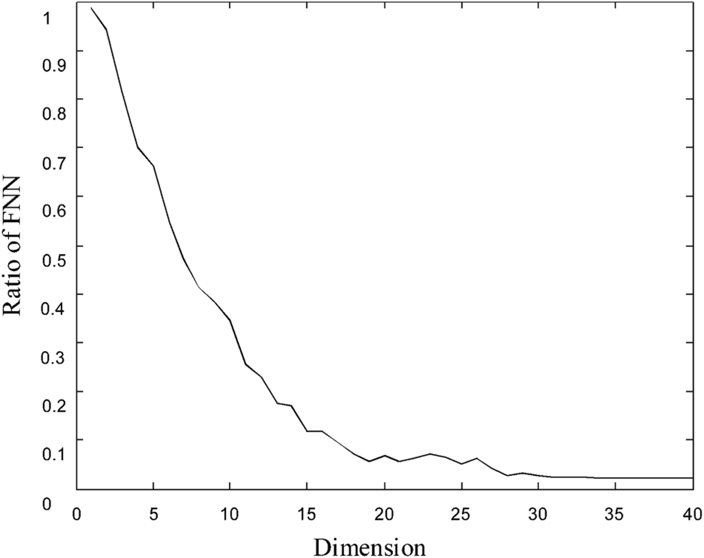
where N − 1 = 279 corresponds to the cut-off frequency of the WB audio. Any two state vectors whose distance is the minimum in the state space are defined as a pair of nearest neighbors. In an appropriate embedding dimension, some neighbors in the state space with a low embedding dimension will no longer be neighbors. This type of nearest neighbors in the low-dimensional space is defined as FNN. With the increase of embedding dimension, FNNs will gradually disappear. So the main idea of FNN method is to examine how the number of FNNs changes as a function of dimension. If the ratio of FNN to all the state vectors does not decrease with the increase of dimension, an appropriate embedding dimension can be determined. The detection method of FNN is detailed in [Reference Rhodes and Morar34]. For an example of the frame of violin signals shown in Fig. 2, the ratio of FNN to all the state vectors as a function of dimension is shown in Fig. 4. If the dimension is larger than 20, the ratio of FNN is not obviously decreasing. The fine spectrum of audio signals is reliably embedded into the state space with the embedding dimension of 20.

Fig. 4. The relationship between ratio of FNN to all the state vectors and state-space dimension.

3) ANALYSIS OF STATE TRAJECTORY

Once the embedding delay Δ i and the embedding dimension m are determined, a state space can be reconstructed from the fine spectrum of audio signals via the delay reconstruction method derived from Formula (7). Here, by mapping the multi-dimensional space into a three-dimensional space, the change of state vectors with the increase of the frequency index i, which are called the state trajectory, can be visualized and guide us in the analysis of audio characteristics. As a visualized example, we select a SWB audio signal of a violin to reconstruct the state space and analyze the state trajectory. The violin signal comes from the sound quality assessment material (SQAM) recordings for subjective tests of audio signals by the European Broadcasting Union [Reference Waters36]. The semitone of violin segment is D4, and the pitch is about 296 Hz. Embedding delay Δ i and embedding dimension m are set to 1 and 3, respectively. Audio signals with the frame length of 20 ms are transformed by MLT. The fine spectrum of audio signals is represented by the normalized MLT coefficients and the state space is reconstructed. The state trajectories of the fine spectra for LF and HF signals are demonstrated in Figs 5 and 6, respectively. It is manifest that the state trajectories turn dispersed with increasing frequency, but nearly all the state vectors for both the HF and LF signals are localized in a certain range to form a hyper-ellipsoidal structure which cannot be predicted by a multivariate linear model. For other orchestral instruments, symphony and pop music from SQAM, the analysis results of state trajectory are similar. It indicates that the state trajectories of audio spectrum are characterized by regular structure and the state vectors are predictable once the state space is properly reconstructed. Moreover, the audio spectra of some percussion music and live background sound are also analyzed in a three-dimensional space. Although the state vectors are scattered in a disorderly way over a certain area, the trajectories of both LF and HF fine spectra show the similar characteristics of randomness.

Fig. 5. Example of state trajectory for LF fine spectrum of audio signal.

Fig. 6. Example of state trajectory for HF fine spectrum of audio signal.

The aforementioned results about state trajectory analysis show that the audio spectrum has significant non-linearity and the state trajectories can be predictable for different audio signals. Once two state vectors are a pair of neighbors in the state space, they will share the similar change processes with the increase of frequency. Inspired by the facts, a prediction model based on NNM is built up in this paper to recover the fine spectrum of high frequencies from that of low frequencies.

1) ESTABLISHING SHAPE SET OF LF FINE SPECTRUM

Using the normalized MLT coefficients in the LF bands C _{norm_mlt} (i), i = 0, …, 279, the state vector describing the LF fine spectrum s _p (i) can be represented as

(8) $$\eqalign{{\bf s}_{\bf p} \lpar i\rpar = & \lcub \vert C_{norm\_mlt} \lpar i\rpar \vert\comma \; \vert C_{norm\_mlt} \lpar i - \Delta i\rpar \vert\comma \; \ldots\comma \; \cr & \vert C_{norm\_mlt} \lpar i - \lpar m - 1\rpar \Delta i\vert\rpar \rcub .}$$

The embedding delay Δ i and the embedding dimension m are computed via the autocorrelation method and the FNN method, respectively, and are used to reconstruct the state space S _p = {s _p (i)| i = (m − 1)Δ i, (m − 1)Δ i + 1, …, 279}. Each vector of S _p can describe the local spectral structure of the LF components. Accordingly, the state space S _p is also defined as the shape set of the LF fine spectrum and provide sufficient information for the dynamic structure of the LF fine spectrum with increasing frequency. It is established every frame with different characteristics of audio spectrum and is not updated by using the predicted MLT coefficients.

2) SEARCHING NEAREST NEIGHBORS

By using the FNN method, the FNNs are eliminated by appropriately increasing the embedding dimension. So the change processes of a given state vector can be estimated by the change of the neighbors. The detailed procedure of searching the nearest neighbors is as follows:

• • Pitch detection: The pitch t ₀ of the band-limited SWB audio signals is computed in the time domain by a normalized cross correlation method. The frequency index i _f of MLT coefficient whose frequency corresponds to the pitch t ₀ can be used for a coarse search of nearest neighbors and is derived as,

  (9) $$i_f =\left\lfloor \displaystyle{1280} \over {t_0}\right\rfloor\comma \;$$
  where ⌊·⌋ represents the rounding function.

• • Coarse searching: The last state vector in the LF components s _p (i), i = 279, is determined as the estimated state vector. And coarse searching will be performed. The state vectors {s _p (i − i _f ), s _p (i − 2i _{f}), s _p (i − 3i _f ),… } are firstly chosen as the initial candidate nearest neighbors of s _p(i). Then, the distance between s _p(i) and each initial candidate nearest neighbor is computed. If the distance is larger than a given threshold, the corresponding candidate nearest neighbor is considered outside the neighborhood of s _p(i) and is discarded. Otherwise, it is determined as a candidate nearest neighbor s ^′ _p(j) through coarse searching.

• • Fine searching: The inner product between s _p(i) and each candidate nearest neighbor {s ^′ _p(j)} are computed one by one. Here, the inner product is adopted instead of the distance measurement due to taking more angle information of state space into consideration. The state vector s _p(i _NN ) which maximizes the modulus of the inner product is selected as the nearest neighbor of s _p(i).i _NN is the index of state vector with the maximal modulus of inner product and defined as,

  (10) $$i_{NN} ={\mathop{\arg\max }\limits_j}\left\{\vert \langle {\bf s}_{\bf p}^{\prime} \lpar j\rpar \comma \; {\bf s}_{\bf p} \lpar i\rpar \rangle\vert \right\}.$$

3) NEAREST NEIGHBOR MAPPING

By maximizing the inner product, the true neighbor of the estimated state vector s _p (i) is determined. The relationship between the neighbor s _p (i _NN ) and the amplitude of the normalized MLT coefficients | C _{norm_mlt} (i _NN + 1)| is presented by a mapping function F[.] as,

(11) $$\vert C_{norm\_mlt} \lpar i_{NN} +1\rpar \vert=F\lsqb {\bf s}_{\bf p} \lpar i_{NN}\rpar \rsqb .$$

Likewise, for the estimated state vector s _p (i), i = 279, the amplitude of the normalized MLT coefficients |C _{norm_mlt} (i + 1)| is predicted by the similar mapping function as follows:

(12) $$\left\vert C_{norm\_mlt} \lpar i+1\rpar \right\vert =F\lsqb {\bf s}_{\bf p} \lpar i\rpar \rsqb .$$

Because the nearest neighbors are very close in the state space, the distance between s _p (i) and s _p (i _NN ) is considered to be small. With the same mapping function, |C _{norm_mlt} (i + 1)| can be approximately estimated by using the output MLT coefficients fed by s _p (i _NN ) as follows:

(13) $$\vert \hat{C}_{norm\_mlt} \lpar i+1\rpar \vert \approx F\lsqb {\bf s}_{\bf p} \lpar i_{NN}\rpar \rsqb =\vert \hat{C}_{norm\_mlt} \lpar i_{NN} +1\rpar \vert .$$

Finally, we should decide whether the frequency corresponding to |Ĉ _{norm_mlt} (i + 1)| rises to the cut-off frequency of 14 kHz. If so, the iterations will be stopped. Otherwise, let i = i + 1, and repeat the steps of searching nearest neighbors and NNM.

4) PRELIMINARY DISCUSSION

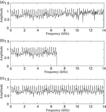
As an example, a segment of audio signal from a violin is preliminarily used to evaluate the proposed prediction method about the fine spectrum of high frequencies. The audio signal has a length of 12 s. The fine spectra of SWB audio signal, WB audio signal, and the predicted audio signal are given in Fig. 8. Analysis result shows that the harmonic structure of the predicted audio signals is improved, and the HF components of the audio signal are well restored. Good results are also achieved in the amplitude prediction of fine spectrum for percussion music and live background sound because the state trajectories of both their HF and LF components share a similar characteristic. However, a challenge appears for some particular audio signals whose LF components have large differences from the HF ones. Take a very high-pitched voice to the accompaniment of bass drums as an example. The noise-like sound produced by drums blurs the harmonic structure in the LF components. If the harmonic structure has emerged from the noisy spectrum in the LF region, the predicted HF components may present characteristics similar to the original ones. Otherwise, the proposed NNM method cannot work well to recover the voice in the HF components. The similar situation may also appear for the audio signals which have individual tonal components in HF regions.

Fig. 8. The comparison of fine spectrum for audio signals from violin. (a) Original spectrum; (b) truncated spectrum; (c) extended spectrum.

In addition, normalized mean-square error is adopted to analyze the influence of embedding delay and embedding dimension over the extension performance of the proposed method and further evaluate the prediction accuracy of HF fine spectrum compared with different BWE methods. The original fine spectrum of HF components is referred to as C _{norm_mlt}(i), i = 280,281,…,559 and its estimated values is Ĉ_{norm_mlt}(i), i = 280,281,…,559. Then, the normalized mean-square error ε _NMSE is defined as,

(14) $$\varepsilon _{NMSE} ={{1 \over 280}{\sum\limits_{i=280}^{559}} {\lpar C_{norm\_mlt} \lpar i\rpar -\hat {C}_{norm\_mlt} \lpar i\rpar \rpar ^2} \over {\sigma _m ^2}}\comma \;$$

where σ _m ² is the variance of C _{norm_mlt} (i). If ε _NMSE is quite large, then the spectral distance induced by BWE is large.

In the proposed BWE method, the autocorrelation method is used to select a proper embedding delay. We experimented with different thresholds and selected an empirical value according to the extension performance of the proposed method. Figure 9 shows little difference of extension performance with different thresholds in autocorrelation method. Therefore, the SSR-based prediction method is not sensitive to the parameter of delay and the traditional threshold (1 − 1/e)R _XX (0) is used. Also, the threshold in the FNN method needs to be analyzed. We experimented with several values of ratio and empirically optimized the threshold under the extension performance. As shown in Fig. 10, the value of ε _NMSE diminished with the decrease of ratio threshold of FNN. But in practice, a small threshold may cause an increase in the computational complexity. According to the preliminary experiments, when the threshold is down to 5%, the embedding dimension selected by the FNN method will be up to over 25. Due to the increase of embedding dimension, the complexity of the SSR module will increase to more than 6 weighted million operations per second (WMOPS) for the worst case, and is almost double the complexity when the threshold is selected to 10%. Therefore, a proper threshold should be selected which considers both extension performance and computational complexity. Here, it is set to 10%.

Fig. 9. ε _NMSE of proposed BWE method with different thresholds in autocorrelation method.

Fig. 10. ε _NMSE of proposed BWE method with different ratio of FNN.

In addition, the prediction accuracy of HF fine spectrum is evaluated and compared with different BWE methods by ε _NMSE . ε _NMSE can guide us in measuring the distortion between the predicted fine spectrum and the original one. In our BWE method, the embedding delay and embedding dimension are adaptively determined by using the autocorrelation method and the FNN method. For the HBE method, the stretching factor is set to 2. And the square function is used as a non-linear function in the TDNP method. Thus, the normalized mean-square error values from four methods are listed in Table 1. It is shown that the prediction error of HBE is the largest because the odd harmonics are not completely reconstructed and the spectral shape of even harmonics is also changed. And the prediction errors from the ST method and TDNP method are in the range of 3.5–5. The TDNP method is suitable for harmonic signals with regards to auditory quality, but the frequency-mixing distortion generated by non-linear processing in time domain leads to a larger error. The ST method directly translates the LF fine spectrum into the HF region. This method reacts sensitively to the spectral characteristics of audio signals. For the violin signals, both the HF and LF components share the strong harmonic characteristics. The moderate distortion is mainly caused by spectral shifting between HF and LF spectra. For some pop music, the noise-like components below 2 kHz generated by accompanying instruments may directly translate into the HF components and lead to more perceptible distortion. In addition, the prediction error of the proposed method is only 2.86. As shown in Fig. 8(c), the HF harmonic structure predicted by the proposed NNM method is substantially consistent with that of the LF spectrum although some artifacts still exist in the HF region. Therefore, it indicates that the proposed BWE method has higher accuracy for spectral prediction compared with conventional BWE methods.

Table 1. Comparison of normalized mean square error for four BWE methods.

1) FEATURE SELECTION

The features extracted from the WB signals are selected for the purpose of differentiating between various audio signals with a different spectral envelope in the HF components. Considering computational complexity, correlation, and independence among data, a 26-dimensional time–frequency feature vector is extracted to describe the auditory perception of the WB audio signals, as shown in Table 2. The precise definition of these specific features of audio signals was given in Reference [Reference Liu, Bao, Jia and Sha25]. The zero-crossing rate F _ZCR and the gradient index F _g are adopted to distinguish the harmonic signal from the noise-like signal [Reference Vary and Martin2]. The sub-band RMS, F _rms (i), i = 0, …, 13, and the flux of sub-band F _flux are used to further represent the spectral envelope information of the WB audio signals. Besides, three MPEG-7 audio descriptors (audio spectrum centroid F _ASC , audio spectrum spread F _ASS and spectrum flatness measurement F _SFM (i), i = 7, …, 13) are also employed to supplement the timbre features [Reference Deng, Simmermacher and Cranefield37,38]. F _ASC describes the position of dominant spectral content in the power spectrum and roughly indicates the timbre of audio signals. F _ASS describes the departure of audio spectrum from F _ASC to depict the auditory brightness of audio signals. F _SFM (i) are defined as the ratio of geometric mean value to algebraic mean value for MLT coefficients in each sub-band in the frequencies from 3.5 to 7 kHz. The values of F _SFM (i) are fixed between 0 and 1. If F _SFM (i) = 0, the signal is totally tonal, otherwise if F _SFM (i) = 1 it is noise-like.

Table 2. Time-frequency features for describing WB audio signals.

In addition, the estimated spectral envelope of HF components F _Y can be represented by RMS of sub-bands, F _rms (i), i = 14, …, 27, in the frequencies from 7 to 14 kHz. In the training of a priori knowledge, the statistical distribution of joint feature vector F _Z = {F _X , F _Y } is computed to guide us in estimating F _Y under the given F _X .

2) TRAINING OF A PRIORI KNOWLEDGE

The block diagram of a priori knowledge training based on HMM is shown in Fig. 11. Firstly, an LBG-based vector quantization method [Reference Lloyd39] is employed to divide the feature space of F _Y into N _s = 16 cells. Each cell is referred to as a model state S _i . According to the state transition process, the actual state transition series {S _i } can be obtained, and the distribution probability of each state P(S _i ) and the one-step transition probability of actual state series P(S _i | S _j ) are computed, respectively. Next, for the joint feature vector F _Z = {F _X ,F _Y }, an independent subset F _Z|Si = {F _X ,F _Y |S _i } is built for each model state. The joint probability density of each state p(F _X,F _Y |S _i ) is modeled by a GMM with 32 mixtures and full covariance matrices, and the parameters of a GMM are trained by the standard expectation–maximization algorithm [Reference Dempster, Laird and Rubin40]. Thereby, P(S _i ), P(S _i |S _j ), and p(F _X , F _Y | S _i ) are used as a priori knowledge for training with an off-line approach.

Fig. 11. Block diagram of a priori knowledge training.

3) ESTIMATION OF THE HF SPECTRAL ENVELOPE

For each state S _i of the HMM model, an MMSE estimator is used to obtain the conditional expectation E{F _Y |S _i ,F _X} of F _Y given the WB features F _X ,

(15) $$E\left\{{\bf F}_{\bf Y} \vert S_i \comma \; {\bf F}_{\bf X}\right\}=\int {\bf F}_{\bf Y} p\lpar {\bf F}_{\bf Y} \vert S_i \comma \; {\bf F}_{\bf X}\rpar d{\bf F}_{\bf Y}\comma \;$$

which can be calculated from the joint probability distribution function p(F _X ,F _Y | S _i ) [Reference Nilsson, Gustafsson, Andersen and Kleijn12].

If the WB feature vector of the m _k ^th frame, F _X (m _k ) = {F _X (m _k − 1), F _X } is known, a posterior probability of the ith state, P(S _i | F _X (m _k )) can be computed in a recursive fashion [Reference Patrick and Fingscheidt41] as follows:

(16) $$\eqalign{P\lpar S_i \vert {\bf F}_{\bf X} \lpar m_k\rpar \rpar &=C\cdot p\lpar {\bf F}_{\bf X} \vert S_i \lpar m_k\rpar \rpar \cr &\quad \cdot \sum\limits_{j=1}^{N_s} P\lpar S_i \lpar m_k \rpar \vert S_j \lpar m_k -1\rpar \rpar \cr & \quad \cdot P\lpar S_j \lpar m_k-1\rpar \vert {\bf F}_{\bf X} \lpar m_k -1\rpar \rpar \comma \; }$$

where the marginal probability density p(F _X (m _k )| S _i (m _k )) of F _X , can be derived from the GMM corresponding to the ith state and C is the normalized factor, which keeps the sum of P(S _i (m _k )| F _X (m _k )) over all the states be equal to 1.

Taking the state transition process into consideration, the HHM-based MMSE estimator can be performed to obtain the optimal estimation of the HF spectral envelope $\hat{\bf F}_{\bf Y}$ and is expressed as,

(17) $$\hat{\bf F}_{\bf Y} =\sum\limits_{i=1}^{Ns} E \left\{{\bf F}_{\bf Y} \vert S_i \comma \; {\bf F}_{\bf X}\right\}P\lpar S_i \vert {\bf F}_{\bf X} \lpar m_k \rpar \rpar .$$

It is worth noting that each state defined by vector quantization is assumed to be stationary and represents the characteristics of one particular SWB audio. The state transition process described by a Markov chain can effectively describe the evolution among “attack, decay, sustain and release” part of a sound in the time domain. Accordingly, the dynamic performance of the BWE method can be improved by using an HMM-based estimator [Reference Song and Martynovich17]. Especially for the transition between different parts of audio, the sudden change of the HF energy caused by misestimating the spectral envelope is reduced.

1) G.722.1 AND G.722.1C CODEC

For the G.722.1 codec, the bandwidth of input signals is 7 kHz, and the sampling rate is 16 kHz. As shown in Fig. 12, an MLT is performed with the frame length of 20 ms and a 50% overlap is used between frames. The MLT coefficients below 7 kHz are uniformly divided into 14 sub-bands. The spectral envelope of each sub-band is scalar quantized and Huffman coded, and 4 bits of control bits are used to indicate the bit allocation and quantization strategy. At last, the Scalar Quantization and Vector Huffman coding (SQVH) of the normalized MLT coefficients is performed.

Fig. 12. Block diagram of G.722.1 encoder.

The inverse process of quantization and encoding is performed in the decoder to reproduce the WB audio signals. However, for some sub-bands with lower energy, no MLT coefficients are transmitted as the fine spectrum due to the limitation of coding bit-rates. To avoid audible artifacts, the decoder reproduces these MLT coefficients using NF for which these coefficients are replaced with values of random sign and amplitude proportional to the sub-band energy.

As an extended mode of G.722.1, the G.722.1C codec adopts the same framework as the G.722.1 main body and is designed to operate with an audio signal sampled at 32 kHz. Since the frequency information transmitted by G.722.1C is double that of G.722.1, G.722.1C must allocate more bits to the LF information in order to facilitate coding efficiency. For G.722.1C at 24 kb/s, only the sub-band energy of the HF components is transmitted to the decoder at about 2 kb/s, while the fine structure of the HF spectrum is almost reproduced by NF. With the increasing of bit-rate, more information describing the fine spectrum is encoded and the quality of the reproduced signals is further enhanced. G.722.1C can be referred to as a non-blind BWE method, which can improve the brightness of the reproduced audio signals at low bit rates. Therefore, it is selected as an important reference method to evaluate the performance of proposed blind BWE method.

2) APPLICATION FRAMEWORK OF THE PROPOSED BWE METHOD

In order to extend the bandwidth of audio signals decoded by G.722.1, the proposed BWE method is embedded into G.722.1 decoder as a separate module. The block diagram of the G.722.1 decoder with BWE is depicted in Fig. 13, and the algorithm is presented in Table 3.

Fig. 13. Block diagram of G.722.1 decoder with BWE.

Table 3. Algorithm of G.722.1 decoder with the BWE function.

The normalized MLT coefficients decoded from the fine spectrum code words according to control bits are used to recover the HF fine spectrum by using the non-linear prediction based on NNM. In addition, a set of features computed from the decoded sub-band energy and the reproduced WB audio is fed into the HMM-based estimator. After the energy adjustment, the regenerated HF components are combined with the original WB audio to form a SWB audio signal via an IMLT. It is worth noting that, because the G.722.1 codec and the proposed BWE method adopt the same time–frequency transform, no additional complexity of time–frequency transform is required in the G.722.1 + BWE scheme.

1) LOG SPECTRAL DISTORTION

For 18 test signals, differences between the differently processed SWB signals and the original SWB signals were compared in terms of LSD measure, which is commonly used for the comparison of the audio spectra. LSD based on the fast Fourier transform power spectrum has been employed for the BWE evaluation in this paper, and its measurement is defined as,

(19) $$d_{LSD} \lpar i\rpar =\sqrt{{1 \over N_{high} -N_{low} +1} \sum\limits_{n=N_{low}}^{N_{high}}\left[10 \log _{10} {P_i \lpar n\rpar \over \hat {P}_i \lpar n\rpar }\right]^2\comma \; }$$

where d _LSD (i) is the LSD value of the ith frame, P _i and $\hat{P}_{i}$ are the power spectra of the original SWB audio signals and the audio signals processed with different methods, respectively. N _high and N _low are the indices corresponding to the upper and lower bound of the frequency band from 7 to 14 kHz. The analysis was performed using a discrete Fourier transformation (DFT) in 20-ms frames without overlapping. The frame-based LSD is averaged over all the frames for each test signal and the mean LSD is used as an objective quality measurement for BWE.

The results of LSD measurement are shown in Fig. 14. Through BWE, the LSD of complicated audio signals is much larger than other types of audio signals. Because various types of instruments are involved in the complicated audio signals, the energy in the HF spectrum is relatively high and not easy to estimate accurately. The distortion of simple audio signals is the smallest, on one hand, because the typical harmonic components in the solo of violin, orchestral instruments, and guitar are easy to recover. On the other hand, the energy attenuation of their HF components is obvious, thus it may lead to a low distortion.

Fig. 14. LSD for different BWE methods.

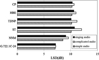
As shown in Fig. 14, the SWB audio reproduced by G.722.1C can achieve the best objective quality for all the three types of audio. The spectral distortion induced by ST is the largest and the mean LSD of ST is about 11 dB. The LSD of ST seems to be different from the normalized mean-square error of ST in Section II. This is because LSD emphasizes the distortion induced by an estimated spectral envelope, instead of the fine spectrum of the extended signals. For the complicated audio with a high energy in the HF bands, some noisy components translated from the components below 2 kHz lead to a higher average distortion. Moreover, LSDs of the TDNP, HBE, and CP methods are similar, and the mean values are around 10.5 dB. NNM method shows a better extension performance than others and the mean LSD is close to 9 dB. Furthermore, the LSD of complicated audio is 1 dB higher than that of simple audio for both the NNM method and the HBE method. Thus, the fine spectrum prediction for complicated audio needs to be further optimized.

2) SEGMENTAL SIGNAL-TO-NOISE RATIO

Besides LSD, SNRseg is also used as an objective quality measurement to evaluate the differences between the reproduced signals and the original signals in the time domain. It is defined as,

(20) $$d_{SNRseg} ={10 \over M} \sum\limits_{m=0}^{M-1} \log_{10} \left(1+{\sum\limits_{n=N\cdot m}^{N\cdot m+N-1} s^2\lpar n\rpar \over \sum\limits_{n=N\cdot m}^{N\cdot m+N-1} \lpar s\lpar n\rpar -\hat {s}\lpar n\rpar \rpar ^2}\right)\comma \;$$

where s(n) and ŝ(n) are the original SWB audio signals and the reproduced audio signals, respectively. N = 640 is the frame length of audio signals and M represents the frame number of each test signal. The SNRseg values of different BWE methods are shown in Fig. 15.

Fig. 15. SNRseg for different BWE methods.

As shown in Fig. 15, the mean SNRseg of complicated audio is the lowest for each method. The CP method does not specially amend the spectral envelope according to the dynamic properties of audio signals, so the SNRseg value is relatively low. The SNRseg values of ST, TDNP, HBE, and NNM show a similar performance, because the similar estimation method based on HMM is employed to shape the spectral envelope of the HF components. The proposed NNM method achieves more than 1 dB improvement over the reference methods, but is inferior to the G.722.1C SWB audio coding.

1) MUSHRA LISTENING TESTS

The listening test was conducted for subjective assessment using MUSHRA methodology recommended by ITU-R BS.1543-1 [44] and was mainly used to grade the degree of audio quality impairment for the BWE methods, SWB audio codec and WB audio codec. In each test case, the listener was presented with the labeled reference, a certain number of test signals, a hidden version of the reference and an anchor. The original SWB audio signal was included as a hidden reference and the low-pass filtered signal with bandwidth of 3.5 kHz as an anchor. The impairments of audio quality for G.722.1 codec at 24 k/s, G.722.1C codec at 24 k/s and 32 kb/s, ST method, HBE method, TDNP method, CP method and proposed NNM method were evaluated for the subjective listening test using the following a 100-point scale: 100–80, Excellent; 80–60, Good; 60–40, Fair; 40–20, Poor; and 20–0, Bad.

15 male and 5 female listeners took part in the test and the age range was from 22 to 30 years old. The test was arranged in the quiet room conforming to the specifications of the ITU-R recommendation BS.1116-1 [45] and only the test attendee was present in the room during the test. Five test signals including pop music, guitar, sax, and drums were selected from the MPEG database [46], and the level of the original test signals and the processed signals was normalized to −26 dB. They were played to both ears through AKG K271 MKII headphones. Each listener compared all the processing types of test signals. In each test case, the listeners could switch at will between the reference signal and any other differently processed signals under test. All the audio signals could be repeated any number of times, and no time limitation is required for giving the response. Before the formal test, another test signal was used for training in order to obtain reliable results. The training phase exposed the listeners to the full range and nature of impairments that would be experienced during the test. Moreover, the listeners were instructed to adjust the sound volume to a suitable level and knew well the test process. During each test case, listeners derived their grade for a given test signal by comparing it to the reference signal, as well as to the other signals, and recorded their assessment of the quality in a previously prepared form. After the test, the comments on the test signals for the listeners were collected and analyzed by the experimenters.

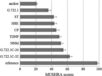
On the assumption that the individual scores meet normal distribution, the mean scores and 95% confidence interval are calculated according to the statistical analysis method mentioned in ITU-R BS.1543-1, and the result for each processing type are illustrated in Fig. 16. The G.722.1C codec at 32 kb/s was considered substantially better than the BWE methods and the WB codec. The performance of the G.722.1C codec at 24 kb/s was a little weaker because the fine spectra of both LF and HF are coarsely reproduced. Due to the same estimation method of HF spectral envelope, ST, HBE, TDNP, and NNM showed a similar performance for extending the audio bandwidth and outperformed the G.722.1 WB audio codec in terms of subjective auditory quality with statistical significance. The proposed NNM method gave marginally better performance than TDNP and performs better than other three BWE methods with statistical significance. But NNM showed slightly impairment compared to the G.722.1C codec at 24 kb/s. In addition, the CP method adopts a different architecture from other methods and also showed a moderate performance.

Fig. 16. Mean subjective scores with 95% confidence intervals for the MUSHRA listening test.

2) CCR LISTENING TESTS

Additionally, a CCR listening test which is similar to the subjective assessment method recommended by ITU-T P.800 [47] was used to pairwise evaluate the differences of audio quality for G.722.1C at 24 kb/s, TDNP, and NNM. In each test case, two differently processed versions of the same test signals were presented to the listeners. Listeners used the following seven-point comparison mean opinion scores (CMOS) to judge the quality of the second audio sample relative to that of the first: 3, much better; 2, better; 1, slightly better; 0, the same; −1, slightly worse; −2, worse; −3 much worse.

A total of 20 listeners who also participated in the CCR test were invited to take part in the test. The test was arranged in the quiet room and the differently processed types of the five MPEG testing signals were played to both ears through AKG K271 MKII headphones for listening tests. Each listener had a short practice before actual tests to adjust the volume setting to a suitable level, and was allowed to repeat each pair of testing data with no time limitation before giving their answers.

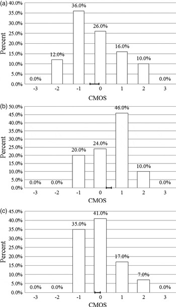
Three groups of tests were presented to each listener. They are the comparison between NNM method and TDNP method, the comparison between G.722.1C codec and TDNP method, and the comparison between NNM method and G.722.1C codec. The distributions of listener rating for each group of tests are shown in Fig. 17. The bars indicate the relative frequencies of the scores given in the comparisons between the two processing methods. Bars on the positive side show preference for the latter method. The mean score for each group of tests is also shown on the horizontal axis with the 95% confidence interval. The proposed NNM method and G.722.1C SWB audio codec showed an improved performance compared with the TDNP method. The SWB audio reproduced by NNM method had the similar quality as the audio signals decoded by G.722.1C. This means that the proposed NNM method is able to enhance the quality of audio signals decoded by G.722.1 and achieves better performance than the TDNP method on average.

Fig. 17. Distributions of listener rating in CCR tests. (a) Comparison between NNM and TDNP. (b) Comparison between TDNP and G.722.1C. (c) Comparison between G.722.1C and NNM.