2.1. Physical human–robot collaboration framework

The essence of pHRC lies in enabling robots to emulate the dynamic characteristics of real-world physical systems by adjusting the virtual dynamic relationship between input forces and output displacements within the system. For instance, admittance control facilitates human–robot interaction by allowing the robot to simulate the behavior of a second-order spring-damping system. A framework for human–robot collaboration based on force controller module is illustrated in Figure 1. This framework comprises three key modules: the force control layer, the robot lower-level control Layer, and the pHRC Module [Reference Chen, Chen, Chen, Lu, Zheng, Wu, Wang, Zhang and Xiong23].

Figure 1. Schematic diagram of pHRC framework.

The force control layer is mainly composed of load identification, gravity/inertial force compensation module, and force controller. Among them, the force controller generates the appropriate velocity ${\mathbf{x}}({\textrm {t}})$ based on the external force ${\textbf {f}}_{\textrm {ext}}$ . This module can be implemented using L-AC, characterized by a second-order spring-damping system, and can also extend to simulate other physical processes, such as shear-thickening fluid dynamics.

The robot lower-level control layer primarily consists of an inverse kinematics solver, a servo controller, and the robot mechanical system. After calculating the robot’s position command in Cartesian space, the desired joint angle ${\textbf {q}}_{\textrm {d}}$ is determined via the inverse kinematics solver, which supplies joint position commands to the servo controller. The controller, in turn, generates the necessary joint torques $\boldsymbol{\tau }$ , based on the velocity commands to drive the robot towards the desired velocity and position.

The inverse kinematics solver typically employs the inverse Jacobian matrix approach to establish the relationship between the joint velocities and the end-effector velocities, as expressed in the following equations:

(1) \begin{equation} \begin{array}{l} \textbf {x}\left ( \textrm {t} \right ) = \textbf {J}\left ( {\textbf {q}\left ( \textrm {t} \right )} \right )\dot {\textbf {q}}\left (\textrm {t} \right )\\ \dot {\textbf {q}}\left ( \textrm {t} \right ) = \textbf {J}{\left ( {\textbf {q}\left ( \textrm {t} \right )} \right )^{ - 1}} \textbf {x}\left ( \textrm {t} \right ) \end{array} \end{equation}

where $\dot {\textbf {q}}\left ( \textrm {t} \right ) \in {\mathbb{R}}{^n}$ represents robot joint velocity vector, with $n$ denoting the number of joints. $\textbf {x}\left ( \textrm {t} \right ) \in {\mathbb{R}}{^m}$ is the velocity vector of the robot’s $m$ -dimensional robot end-effector in Cartesian space, and $\textbf {J}{\left ( {\textbf {q}\left ( \textrm {t} \right )} \right ) }\in {{\mathbb{R}}^{m \times n}}$ corresponds to the Jacobian matrix.

A major limitation of the traditional inverse Jacobian method lies in its inability to handle situations when the robot operates near or at a singularity. From the perspective of linear equations, a robot approaching a singularity results in an ill-conditioned Jacobian matrix, where even a small $\textbf {x}\left ( \textrm {t} \right )$ can lead to disproportionately large $\dot {\textbf {q}}\left ( \textrm {t} \right )$ , making the system sensitive to numerical errors. At a singularity, the equations may either have no solutions or infinitely many solutions.

To address the issues of singularities and redundancy, the pseudo-inverse of the Jacobian matrix can be calculated using the damped least squares method, as shown in the equation below:

(2) \begin{equation} \textbf {J}{\left ( \textbf {q} \right )^\dagger } = \textbf {J}{\left ( \textbf {q} \right )^T}{\left ( {\textbf {J}\left ( \textbf {q} \right )\textbf {J}{{\left ( \textbf {q} \right )}^T} + {\lambda _d}^2 \textbf {I}} \right )^{ - 1}} \end{equation}

where ${\lambda _d} \gt 0$ is a small damping factor introduced to mitigate the effects of singularities. As the robot approaches a singularity, this damping term reduces the sensitivity of the system to ill-conditioned Jacobian.

Using the pseudo-inverse of the Jacobian matrix in Eq. (2), the inverse kinematics relation of the robot can be calculated:

(3) \begin{equation} {\dot {\textbf {q}}_{\textrm {d}}}\left ( {\textrm {t}} \right ) = \textbf {J}{\left ( \textbf {q} \right )^\dagger }{\dot {\bar {\textbf {x}}}}\left ( {\textrm {t}} \right ) \end{equation}

where ${\dot {\bar {\textbf {x}}}}\left ( {\textrm {t}} \right )$ refers to the target velocity of the robot’s end-effector corresponding to the virtual dynamics, and ${\dot {\textbf {q}}_{\textrm {d}}}\left ( {\textrm {t}} \right )$ is the configuration space velocity to reach velocity ${\dot {\bar {\textbf {x}}}}\left ( {\textrm {t}} \right )$ .

The pHRC module captures and abstracts the interactive relationship between the human operator and the robot. It defines the external force ${\textbf {f}}_{\textrm {ext}}$ , as a combination of the feedback force generated by the operator ${\textbf {f}}_{\textrm {h}}$ and the force exerted by the environment on the robot ${\textbf {f}}_{\textrm {env}}$ . This abstraction enables closed-loop control by interpreting the physical interaction as a force signal. During the collaboration process, the robot operates outside physical cages, sharing the workspace with the operator. However, environmental disturbances can manifest as random impacts on ${\textbf {f}}_{\textrm {ext}}$ , potentially causing the robot to shake or make unintended movements. Consequently, the virtual dynamics model must not only adapt to the operator’s intended traction forces but also actively resist such disturbances to ensure collaboration safety.

2.2. pHRC framework based on L-AC and SFC

As previously discussed, the L-AC algorithm can be employed to design the force control module. Given that the multi-dimensional motion of the robot can be represented as a linear superposition of single-dimensional motions [Reference Chen, Chen, Chen, Lu, Zheng, Wu, Wang, Zhang and Xiong23], L-AC can be defined as follows:

(4) \begin{equation} {m_A}\ddot x\left ( t \right ) + {\mu _A}\dot x\left ( t \right ) = {f_{{\textrm {ext}}}}\left ( t \right ) \end{equation}

where ${{m}}_{{A}}$ and ${\mu _A}$ denote the virtual inertia and damping parameters of the controller, respectively, both of which must be positive. The term ${f_{{\textrm {ext}}}}\left ( t \right )$ represents the external force applied to the robot’s end-effector, while $\ddot x$ and $\dot x$ denote the acceleration and velocity, respectively.

Figure 2. The relationship between velocity (X-axis) and normalized nonlinear damping force(Y-axis).

The relationship between the input and output of L-AC is linear, as indicated in Eq. (4). Consequently, L-AC cannot differentiate between traction and impact forces, which limits its effectiveness in resisting random impacts.

To overcome this limitation, a virtual dynamics control model based on shear-thickened fluid (STF) characteristics was proposed in ref. [Reference Chen, Chen, Chen, Lu, Zheng, Wu, Wang, Zhang and Xiong23]. This model enables the robot to simulate the dynamics of solid–liquid phase transitions in STFs, behaving like a soft liquid under light contact while becoming rigid when subjected to strong impacts. The dynamic equation for this model can be expressed as follows:

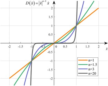
(5) \begin{equation} m\ddot x\left ( t \right ) + \mu {\left | {\dot x\left ( t \right )} \right |^{n - 1}}\dot x\left ( t \right ) = {f_{{\textrm {ext}}}}\left ( t \right ) \end{equation}

where ${D( {\dot x} ) = \mu { | {\dot x} |^{n - 1}}\dot x}$ represents the nonlinear damping term, which can be derived from the constitutive equation of STFs. $m \gt 0$ is the virtual inertial term, and $\mu \ge 0$ a constant that characterizes the internal flow resistance properties of the material.

The principle behind the STF-based control is to indirectly adjust the nonlinear term within the controller through the external force $f_{{\textrm {ext}}}$ , enabling the system to resist impacts while following the operator’s traction. Specifically, the nonlinear damping term increases with the system’s speed, allowing for rapid energy dissipation and enhanced impact resistance.

The behavior of the nonlinear damping force in relation to velocity is illustrated in Figure 2. The $X$ -axis represents velocity $\dot x$ , while the $Y$ -axis shows the nonlinear damping force ( $D( {\dot x} ) = \mu { | {\dot x} |^{n - 1}}\dot x$ ), with $\mu$ set to 1 and $n$ taking values of 1, 1.5, 3, and 20. The function $D( {\dot x} )$ is symmetric about the origin. For $n = 1$ , the graph is a straight line, indicating that the control system reduces to linear admittance control. As $n \gt 1$ , the curve steepens with increasing velocity, suggesting that when the system experiences a large external force impact, the damping force correspondingly increases to dissipate energy and maintain stability in human–robot interaction. It is important to note that while this effect becomes more pronounced with higher values of $n$ , excessively high values may not always yield optimal performance.

2.3. Limitations of designing virtual dynamics controller based on SFC

As previously mentioned, while LAC struggles to differentiate between traction and impact forces and effectively counter random impacts, the SFC successfully addresses these challenges. However, the SFC approach presents several limitations that require further investigation.

Figure 3. Three phases of typical STFs and relevant parameters of its piecewise model. The X-axis represents shear rate $\dot \gamma$ , while the Y-axis represents apparent viscosity $\eta$ .

Figure 4. Comparison of the effects of nonlinear damping forces in the ISFC and SFC with parameters $\mu {\textrm { = }}1$ , $n = 3$ , and ${\eta _0} = 5$ .

One issue with the SFC system is its delayed response when halting movement after the removal of traction force, which compromises the robot’s ability to stop promptly in response to operator commands. Figure 2 illustrates nonlinear damping force behavior ( $n \gt 1$ ) at low system velocities ( $\dot x \lt 1$ ). The damping force significantly decreases as system speed diminishes, nearing negligible levels as velocity approaches zero. This effect is exacerbated with increasing values of $n$ . Consequently, the system continues to move after traction force is removed, owing to the notably reduced energy dissipation capability of the SFC’s near-zero damping term. This limitation adversely affects controller performance in pHRC, undermining the precise execution of operator-intended movements and potentially threatening the safety of both operators and robots. Further simulations and experiments will explore this phenomenon in detail.

Additionally, SFC is incompatible with dual-arm robot collaborative control algorithms, complicating its application in such systems. Precise task execution in dual-arm robots relies heavily on the relative positions and orientations of the end effectors. As noted, SFC-equipped robots cannot immediately halt after traction force is removed. This limitation hinders the ability to meet the stringent precision control requirements of dual-arm systems. For instance, when a human collaborates with dual-arm robots in material handling tasks, unintentional robotic movements can accumulate, significantly impairing system stability and potentially resulting in task failure.

This paper proposes an improvement to the existing SFC algorithm by incorporating the shear-thinning properties of shear-thickening fluids to address the aforementioned issues. This characteristic allows the system to maintain a certain level of nonlinear damping at low speeds, enabling the robot to quickly stop moving when traction is removed, thereby preserving system stability.

3.1. Design of the ISFC

As discussed earlier, the traditional SFC algorithm only considers the fluid characteristics during shear thickening, resulting in insufficient performance of the controller at low shear rates. According to ref. [Reference Li, Lyu, Yuan, Dong and Dai25], the apparent viscosity of STFs exhibits three distinct zones as the shear rate increases: (1) shear thinning, (2) shear thickening, and (3) shear thinning again, as illustrated in Figure 3. In the initial phase $\left ( {\dot \gamma \le {{\dot \gamma }_c}} \right )$ , as the shear rate increases, the STFs system exhibits shear-thinning behavior, causing the apparent viscosity to decrease from the initial value $\eta _0$ to the minimum value $\eta _c$ . In the intermediate phase $\left ( {{{\dot \gamma }_c} \le \dot \gamma \le {{\dot \gamma }_{\max }}} \right )$ , as the shear rate continues to increase, the fluid exhibits shear thickening behavior, causing the apparent viscosity to reach its peak value $\eta _{\max }$ . Finally, in the third phase $\left ( {\dot \gamma \ge {{\dot \gamma }_{\max }}} \right )$ , the apparent viscosity decreases dramatically. This paper argues that, in the low shear rate range, the SFC algorithm should account for the shear-thinning effect and the corresponding changes in apparent viscosity from a specific initial viscosity value.

The constitutive equation for Zone II of STFs can be modeled using the power-law model [Reference Wei, Lin and Sun24]:

(6) \begin{equation} \tau = \left ( {\mu {{\left | {\dot \gamma } \right |}^{n - 1}} + a} \right )\dot \gamma \end{equation}

where $\tau$ represents the stress tensor, $\eta = \mu {\left | {\dot \gamma } \right |^{n - 1}} + a$ denotes the apparent viscosity, $\mu$ is a material-dependent constant, $a$ is a curve adjustment parameter, $\dot \gamma$ is the shear rate, and $n$ is the power-law index $\left ( {n \gt 1} \right )$ .

Inspired by the constitutive Eq. (6), the shear thickening behavior is applied to the nonlinear damping term of the controller. $\dot \gamma$ and $\tau$ are replaced by $\dot x$ and $D( {\dot x} )$ , respectively. Based on the shear thinning characteristics of the fluid in Zone I of Figure 3, the adjustment parameter $a$ is further defined as $a = {\eta _0}{e^{ - | {\dot x} |}}$ . The dynamic equation of the controller’s viscosity term, modeled using the improved shear-thickening fluid, is given by:

(7) \begin{equation} D( {\dot x} ) = \left ( {\mu {{ | {\dot x} |}^{n - 1}} + {\eta _0}{e^{ - | {\dot x} |}}} \right )\dot x \end{equation}

Combining Eq. (7) with Eq. (5), the proposed ISFC can be expressed as:

(8) \begin{equation} \left \{ \begin{array}{l} m\ddot x + \left ( {\mu {{ | {\dot x} |}^{n - 1}} + {\eta _0}{e^{ - | {\dot x} |}}} \right )\dot x = {f_{{\textrm {ext}}}}\\[3pt] \dot {\bar {x}}= \lambda \dot x\\[3pt]\bar x = \int {\dot {\bar {x}} dt} \end{array} \right . \end{equation}

where $D( {\dot x} ) = \left ( {\mu {{ | {\dot x} |}^{n - 1}} + {\eta _0}{e^{ - | {\dot x} |}}} \right )\dot x$ denotes the nonlinear damping term. ${\eta _0} \gt 0$ is the initial value of the apparent viscosity when the fluid undergoes shear thinning behavior, $\lambda$ is a gain term used to regulate the system output, and $\bar {x}$ is the output of the ISFC.

The nonlinear damping term is derived from the constitutive equation of the fluid and incorporates two key components. First, $\mu { | {\dot x} |^{n - 1}}$ represents a power-law model of apparent viscosity, characterizing the shear-thickening behavior of the fluid. This model enables the system to replicate the dynamic properties of STFs, ensuring both compliance and resilience against impacts. Second, ${\eta _0}{e^{ - | {\dot x} |}}$ accounts for viscosity variations, specifically modeling the shear-thinning behavior observed in Zone I of Figure 3. This modification addresses the limitation of inadequate damping force at low velocities, mitigating unpredictable movements in the system when the traction force from a human operator is withdrawn. Figure 4 presents a comparative analysis of the nonlinear damping terms between the proposed ISFC algorithm and the conventional SFC, with the parameter $n$ set to 3. It can be observed that, within the velocity range close to zero (from −1.3 to 1.3), ISFC generates a higher damping force compared to SFC. This indicates that when the human collaborator withdraws the traction force, the proposed ISFC algorithm can dissipate the remaining energy of the system more rapidly, allowing the robot to comply with the human’s intentions and reach the desired position.

The gain parameter $\lambda$ is introduced to scale the velocity output according to the robot’s operational constraints and human comfort levels, ensuring safe interaction velocities while maintaining system responsiveness.

3.2. Safety validation of the ISFC

The ISFC exhibits several essential properties – nonlinear velocity ratio, stability, and passivity – that ensure its practical applicability in robotic systems. The key characteristics are detailed as follows:

(1) Property 1: Nonlinear spatial velocity ratio.

Proof.

In the phase plane of a nonlinear system [Reference Slotine and Li26], the dynamics of the system in Eq. (8) can be represented as:

(9) \begin{equation} \left \{ \begin{array}{l} {{\dot p}_1} = {p_2}\\[3pt] {{\dot p}_2} = \frac {{ - \left ( {\mu {{\left | {{p_2}} \right |}^{n - 1}} + {\eta _0}{e^{ - \left | {{p_2}} \right |}}} \right ){p_2}}}{m} \end{array} \right . \end{equation}

where $p_1$ represents the position state and $p_2$ the velocity state within the phase plane.

The spatial velocity ratio of the phase trajectory is given by:

(10) \begin{equation} {R_{sv}} = \frac {{d{p_2}}}{{dt}}\frac {{dt}}{{d{p_1}}} = \frac {{{{\dot p}_2}}}{{{{\dot p}_1}}} = - \frac {{\mu {{\left | {{p_2}} \right |}^{n - 1}} + {\eta _0}{e^{ - \left | {{p_2}} \right |}}}}{m}. \end{equation}

From this equation, it is evident that when the velocity $p_2$ exceeds 1, the relative magnitude of the spatial velocity ratio of a linear ISFC system ( $n=1$ ) and a nonlinear ISFC system ( $n\gt 1$ ) can be expressed as:

(11) \begin{equation} {R_{sv}}\left | {_{{p_2} \ge 1,n \gt 1}} \right . \ge {R_{sv}}\left | {_{{p_2} \ge 1,n{\textrm { = }}1}} \right . \end{equation}

Thus, when the velocity is high ( $p_2 \ge 1$ ), the spatial velocity of the nonlinear system ( $n\gt 1$ ) is greater than that of the linear system ( $n=1$ ).

The spatial velocity ratio primarily investigates the convergence behavior of position and velocity states in the free motion stage. A larger nonlinear spatial velocity ratio indicates that the rate of change of velocity state ( ${d{p_2}} \mathord { /{\vphantom {{d{p_2}} {dt}}} .} {dt}$ ) is relatively faster than the rate of change of position state ( ${{d{p_1}} \mathord { /{\vphantom {{d{p_1}} {dt}}} .} {dt}}$ ) at a given point on the phase trajectory, which can ensure the stability of the system in the free state without external forces.

(2) Property 2: Stability.

Proof.

Consider the system described by Eq. (8), assuming that $m \gt 0$ , $\mu \gt 0$ , $n \gt 0$ , and ${\eta _0} \gt 0$ and a constant input force $f_{{\textrm {ext}}}$ . Under these conditions, the system has a unique equilibrium point, which is globally asymptotically stable.

Define:

(12) \begin{equation} f ( {\dot p} ) = \left ( {\mu {{ | {\dot p} |}^{n - 1}} + {\eta _0}e^{ { - | {\dot p} |}}} \right )\dot p \end{equation}

Since $f\left ( { - \dot p} \right ) = - f ( {\dot p} )$ , $f$ is an odd-symmetric function. The derivative of $f ( {\dot p} )$ with respect to $\dot p$ is:

(13) \begin{equation} f'(\dot {p}) = \mu n |\dot {p}|^{n-1} + ( 1 - |\dot {p}| ) {\eta _0} e^{-|\dot {p}|} \end{equation}

In deriving Eq. (13), careful consideration is given to the piecewise nature of the absolute value function $ |\dot {p}|$ . For $ \dot {p} \geq 0$ , we have $ |\dot {p}| = \dot {p}$ and $ \frac {d}{d\dot {p}}|\dot {p}| = 1$ . For $ \dot {p} \lt 0$ , we have $ |\dot {p}| = -\dot {p}$ and $ \frac {d}{d\dot {p}}|\dot {p}| = -1$ . The derivation is first performed for the case $ \dot {p} \geq 0$ and then extended to the entire domain using the odd symmetry property $ f(-\dot {p}) = -f(\dot {p})$ , which ensures the derivative $ f'(\dot {p})$ is well-defined and positive under the given conditions for all $ \dot {p} \in \mathbb{R}$ .

We partition the domain into two intervals and analyze the strict positivity of $ f'(\dot {p})$ in each. For $ |\dot {p}| \leq 1$ , both terms in $ f'(\dot {p}) = \mu n |\dot {p}|^{n-1} + (1 - |\dot {p}|) \eta _0 e^{-|\dot {p}|}$ are non-negative: $ \mu n |\dot {p}|^{n-1} \geq 0$ due to $ \mu , n \gt 0$ , and $ (1 - |\dot {p}|) \eta _0 e^{-|\dot {p}|} \geq 0$ since $ |\dot {p}| \leq 1$ . At $ \dot {p} = 0$ , $ f'(0) = \eta _0 \gt 0$ ; for $ 0 \lt |\dot {p}| \leq 1$ , the sum remains strictly positive as both terms cannot vanish simultaneously. For $ |\dot {p}| \gt 1$ , define $ t = |\dot {p}|$ and rewrite $ f'(\dot {p}) \geq \mu n t^{n-1} - \eta _0 t e^{-t}$ (since $ 1 - t \geq -t$ ). The auxiliary function $ g(t) = \mu n t^{n-1} - \eta _0 t e^{-t}$ satisfies $ \lim _{t \to \infty } g(t) = +\infty$ due to exponential dominance ( $ \lim _{t \to \infty } \frac {\mu n t^{n-1}}{\eta _0 t e^{-t}} = +\infty$ ). Its derivative $ g'(t) = \mu n(n-1)t^{n-2} + \eta _0 (t-1) e^{-t}$ is positive for $ t \gt 1$ because $ \mu n(n-1)t^{n-2} \gt 0$ and $ \eta _0 (t-1) e^{-t} \gt 0$ , rendering $ g(t)$ strictly increasing. At the boundary $ t = 1$ , $ g(1) = \mu n - \eta _0/e$ , which is positive if $ \mu n \gt \eta _0/e$ . Consequently, $ g(t) \gt 0$ for all $ t \gt 1$ , ensuring $ f'(\dot {p}) \gt 0$ globally under this condition. By virtue of the strict monotonicity of $f(\dot {p})$ established above, there exists a unique solution $\dot {p^\ast }$ for any constant external force input $f_{\mathrm{ext}}$ .

By defining a new variable $s = \dot p - {\dot p^*}$ , the equilibrium point is shifted to the origin, and the system becomes:

(14) \begin{equation} m\dot s + \left ( {\mu {{ | s |}^{n - 1}} + {\eta _0}{e^{ - | s |}}} \right )s = 0 \end{equation}

Consider the Lyapunov function:

(15) \begin{equation} V(s) = {s^2} \end{equation}

The derivative of $V$ along the system trajectory is:

(16) \begin{equation} \dot V(s) = - \frac {{2\left ( {\mu {{| s|}^{n - 1}} + {\eta _0}{e^{ - | s |}}} \right ){s^2}}}{m} \end{equation}

Since $m \gt 0$ , $\mu \gt 0$ , $n \gt 0$ , ${\eta _0} \gt 0$ , it can be seen that $\dot V (s)$ is negative definite. By Lyapunov’s stability theorem, the system is globally asymptotically stable.

The ISFC must ensure that the robot’s speed tracking is stable, enabling the robot to perform tasks such as human–robot collaboration involving dragging.

Stability ensures that the robot’s movements remain consistent and controlled, even during tasks involving human–robot interaction and continuous external forces.

(3) Property 3: Passivity.

The stability of ISFC under constant external forces has been analyzed. To evaluate stability under other external force disturbances, energy dissipation must be considered. The passivity of the ISFC ensures the system does not accumulate energy uncontrollably, thereby enhancing reliability.

Proof.

Define a Lyapunov-like function:

(17) \begin{equation} \dot {U}(\dot {p}) = \frac {1}{2} m \ \dot {p}^2 \end{equation}

The system’s power form is expressed as:

(18) \begin{equation} \frac {d}{{dt}}\left ( {\dot U( {\dot x} )} \right ) = \dot x{f_{ext}} - h( {\dot x} ) \end{equation}

where $h( {\dot x} ) = \left ( {\mu {{ | {\dot x} |}^{n - 1}} + {\eta _0}{e^{ - | {\dot x} |}}} \right ){\dot x^2}$ represents the dissipated power. Since $h( {\dot x} ) \ge 0$ and ${1 \mathord {\left / {\vphantom {1 2}} \right . } 2}m{\dot x^2}$ has a lower bound, the system is dissipative. Furthermore, the non-negative dissipation term confirms that the system is passive.

During human–robot collaboration, disturbances or transitions from non-contact to contact states can occur. The passivity of ISFC ensures that external forces are dissipated, maintaining stability and safety.

3.3. Discretization of the ISFC

The ISFC discussed previously operates in continuous time; however, in practical applications, the constraints of hardware and software often necessitate the use of discrete time parameters. The discretized ISFC can be represented as follows:

(19) \begin{equation} \left \{ \begin{array}{l} \ddot x\left ( t \right ) = {m^{ - 1}}\left ( {{f_{ext}}\left ( t \right ) - D\left ( {\dot x\left ( {t - \Delta t} \right )} \right )} \right )\\[3pt] \dot {\bar x}\left ( t \right ) = \lambda \left ( {\dot x\left ( {t - \Delta t} \right ) + \ddot x\left ( t \right )\Delta t} \right )\\[3pt] \bar x\left ( t \right ) = x\left ( {t - \Delta t} \right ) + \dot { \bar x}\left ( t \right )\Delta t \end{array} \right . \end{equation}

where $\Delta t$ denotes the sampling time of the system, and the term $D\left ( \dot {x}(t - \Delta t) \right )$ is defined as:

\begin{equation*} \left ( \mu \left | \dot {x}(t - \Delta t) \right |^{n - 1} + \eta _0 e^{-\left | \dot {x}(t - \Delta t) \right |} \right ) \dot {x}(t - \Delta t) \end{equation*}

By iterating Eq. (19) over discrete time steps, the discretized ISFC can compute the robot input $\bar x\left ( t \right )$ at each step based on the current system state $\ddot x\left ( t \right )$ and past information $ \dot {x}(t - \Delta t)$ . This approach facilitates the implementation of the controller in practical robot control systems with discrete-time updates.

6.1. Experimental setup

The experimental setup consists of two ROKAE xMate3 Pro 7-DOF manipulators, two KWR75B force/torque sensors (manufactured by Kunwei Sensing Technology), an industrial PC, and two Rochu grippers. The force sensors are mounted between the robot end flanges and the grippers, enabling direct measurement of the external forces $ \mathbf{f}_{\text{ext},1}$ and $ \mathbf{f}_{\text{ext},2}$ at each end-effector. This configuration allows the total external force acting on the system to be naturally distributed and measured without requiring explicit force decomposition algorithms. Operating at a sampling rate of 1,000 Hz, the sensors relay force information back to the controller. The controller comprises a control module, a dual-arm robot coordination module, and a communication module, with a total communication cycle of 0.001 s. Furthermore, output signals from the sensors undergo the load/gravity compensation algorithm, although this detail is not the primary focus of this paper.

6.2. Comparison of performance between ISFC, SFC, and L-AC for a single robot

In this experiment, the control parameters for ISFC, SFC, and L-AC remain consistent with those utilized in the simulations, as detailed in Table I. The maximum comfortable operating force ${\textrm {f}}_{\textrm {h}}$ that is comfortable for a human operator to be approximately 3 N, while the impact force exerted by the robot is assumed not to exceed 30 N.

The experiment focuses on the simultaneous impact and traction phase, which comprehensively compares the performances of L-AC, SFC, and ISFC.

Simultaneous impact and traction phase: In this phase, to comprehensively assess the performance of the three control methods in handling both traction and impact forces, a traction force in the $Y$ -axis positive direction allows easy robot pushing, with a sudden impact in the negative $Z$ -axis during traction. Note that only forces are considered in these experiments, to prevent the cup from toppling due to potential changes in the robot’s orientation. As shown in Figure 8, in the L-AC scenario, the coffee spills due to an external force impact, whereas in the SFC and ISFC scenarios, the coffee remains intact. Figure 9b illustrates that L-AC incurs a 0.23 m/s velocity jump, causing coffee spilling, while the peak velocities for SFC and ISFC are around 0.047 m/s, with gradual velocity remission post-impact, avoiding sudden jumps. This behavior stems from the dynamic characteristics of shear thickening in the nonlinear damping term. Figure 9 presents the velocity and position variations of the robot’s end-effector. When subjected to a traction force not exceeding 2 N, the robot is pushed stably and smoothly, maintaining a velocity below 0.04 m/s, which demonstrates compliant response characteristics across all three control systems suitable for pHRC.

Figure 8. Snapshots of the simultaneous impact and traction phase.

Figure 9. The external force (Simultaneous impact and traction) acting on the manipulator during the impact phase, as well as the velocity and position of the end-effector. (a)–(c) L-AC. (d)–(f) SFC. (g)–(i) ISFC.

The limitation of SFC is quantitatively evident in Figure 9(e) and (h). Upon removal of the impact force at $t \approx 4.563 \, \text{s}$ , SFC exhibits slow convergence ( $T_{\text{conv}} = 8.29 \pm 0.55 \, \text{s}$ , mean $\pm$ std, $n=10$ trials, $f_{\text{impact}} \approx 18 \, \text{N}$ ), leading to substantial residual displacement ( $D_{\text{res}} = 13.21 \pm 1.1 \, \text{mm}$ ) as the robot drifts unintentionally (Figure 8, Snapshot 4; Figure 9(e)). This drift poses a collision risk and impedes precise task execution. In stark contrast, ISFC (Figure 9(h,i)) achieves rapid stabilization ( $T_{\text{conv}} = 0.50 \pm 0.08 \, \text{s}$ ) with minimal residual displacement ( $D_{\text{res}} = 6.7 \pm 0.3 \, \text{mm}$ ). While both controllers exhibit low overshoot ratios ( $R_{\text{over}} = 0.28 \pm 0.02$ for SFC vs. $0.27 \pm 0.01$ for ISFC), the dramatic improvements in $T_{\text{conv}}$ (94.1% reduction) and $D_{\text{res}}$ (49.3% reduction) conclusively demonstrate ISFC’s resolution of SFC’s low-speed stability defect. These experimental metrics (Table II) align with the simulated behavior in Figure 7 and validate the efficacy of the $\eta _{0}e^{-|\dot {x}|}$ damping term.

Table II. Experimental comparison of low-speed stability metrics (SFC vs. ISFC, $f_{\text{ext}} \approx 18\text{N}$ , $n=10$ trials).

Figure 10. Snapshots of the traction phase of HDRC.

In conclusion, the proposed ISFC algorithm can be effectively applied in pHRC, resisting random impacts and maintaining low-velocity stability. These advantages are attributed to the nonlinear damping term of the ISFC, which accounts for viscosity changes during shear thinning in shear-thickening fluids (STFs). This allows the system to maintain relatively high damping at low velocities, preventing unintended movements of the robot, as quantitatively demonstrated by the 94% reduction in convergence time and 49% reduction in residual displacement compared to SFC (Table II).

6.3. Comparison of performance between ISFC, SFC, and L-AC for a dual-arm robot

Traction and Impact Phase of HDRC: As illustrated in Figure 10, snapshots are presented from the experimental phase of the cooperative water-carrying traction phase between robots and a human operator. Impacts are randomly applied to the end-effectors of Robot 1 and Robot 2.

The experimental results are depicted in Figure 11. The external forces are denoted as $\textbf {f}_{{\textrm {ext1}}}$ and $\textbf {f}_{{\textrm {ext2}}}$ , as illustrated in Figure 11(a) and (b). The trajectories of the two robots’ end-effectors are depicted in Figure 11(c), consistent with the snapshots shown in Figure 10. The controller proposed in Section IV enables dual-arm robot to collaborate with human to complete tasks. Furthermore, the output velocities of the two robots, as illustrated in Figure 11(d) and (e), demonstrate a positive correlation with the external forces, indicating that the robots can respond smoothly to the intentions of the human operator.

Figure 11. The results of the collaborative traction and impact phase between the dual-arm robot and the human operator. (a) and (b) External forces $f_{{\textrm {ext1}}}$ and $f_{{\textrm {ext2}}}$ . (c) Three-dimensional positions of robots 1 and 2. (d) and (e) Output velocities of robots 1 and 2. (f) Position synchronous error.

The fluctuations in velocity observed in Figure 11(d) and (e) result from these impacts. Notably, despite the presence of impacts, the peak velocity generated remains within the safe range for human–robot collaboration, not exceeding 0.1 m/s. To further illustrate the advantages of the algorithm, the concept of position synchronous error is introduced. In this paper, position synchronous error is defined as the difference between the positions of Robot 1 and Robot 2 at each communication cycle, with the initial position deviation subtracted. The position synchronous errors of the two robots in the $X$ , $Y$ , and $Z$ directions are illustrated in Figure 11f. The position synchronous error is less than 8 mm, indicating excellent synchronization performance of the controller. The error reaches its maximum when the absolute value of the instantaneous velocity is highest, with a peak of 7.05 mm in the $Z$ -direction. However, once the impact dissipates, the position synchronous error decreases to a lower numerical range. Moreover, the position synchronous error is positively correlated with the output velocity, which is due to the limitations of the system’s communication cycle.

The experimental results demonstrate that the proposed ISFC algorithm effectively resists random impacts and maintains stability under low-velocity conditions. When integrated with the HDRC framework, the ISFC can be deployed on dual-arm robots to achieve stable operations that are resilient to impacts, thereby facilitating reliable collaboration between human operators and dual-arm robots in the presence of disturbances.