


1. Introduction
Stochastic gradient descent (SGD) is traditionally focused on finding the minimum value of a function, also called the objective function in the optimization literature [Reference Ghadimi and Lan15, Reference Jin, Netrapalli, Ge, Kakade and Jordan21, Reference Mertikopoulos, Hallak, Kavis and Cevher25, Reference Robbins and Monro30]. It has proven to be an extremely effective method in tackling hard problems in multiple fields such as machine learning [Reference Bottou, Curtis and Nocedal3], statistics [Reference Toulis and Airoldi31], and electrical engineering [Reference Golmant, Vemuri, Yao, Feinberg, Gholami, Rothauge, Mahoney and Gonzalez17].
The SGD algorithm and some of its properties are now well known especially in the context of machine learning. The iterative version of the SGD algorithm is given as
 \begin{align}x_{k+1}=x_k -\gamma_k \nabla g(x_k)-\gamma_k \xi(x_k)_{k+1}, \ \textrm{for } k=0,1,2,\ldots,\end{align}
where $\gamma_k$
is called the step size (it is possible to choose
$\gamma_k$
is called the step size (it is possible to choose $\gamma_k=\gamma$
for all k),
$\gamma_k=\gamma$
for all k), $g(\! \cdot \!)$
the objective function (the function for which we want the optimum) and
$g(\! \cdot \!)$
the objective function (the function for which we want the optimum) and $\xi(x_k)_{k+1}$
is the error term that may or may not depend on the current point
$\xi(x_k)_{k+1}$
is the error term that may or may not depend on the current point $x_k$
. The SGD algorithm can be thought of as a stochastic generalization of the gradient descent (GD) algorithm, one of the oldest algorithms for optimization. One of the most popular methods for performing SGD in practice is to perform SGD via minibatching [Reference Bottou4], i.e. select a subset of the data available randomly and then perform the iteration step. From this point onward, we refer to this algorithm as minibatch SGD.
$x_k$
. The SGD algorithm can be thought of as a stochastic generalization of the gradient descent (GD) algorithm, one of the oldest algorithms for optimization. One of the most popular methods for performing SGD in practice is to perform SGD via minibatching [Reference Bottou4], i.e. select a subset of the data available randomly and then perform the iteration step. From this point onward, we refer to this algorithm as minibatch SGD.
Though initially proposed to remedy the computational problem of gradient descent, recent studies have shown that minibatch SGD has the property of inducing an implicit regularization, which prevents the over-parametrized models from converging to the minima [Reference Hoffer, Hubara and Soudry19, Reference Zhang, Bengio, Hardt, Recht and Vinyals35]. This phenomenon leads to an investigation [Reference Wu, Hu, Xiong, Huan, Braverman and Zhu33], which introduced a version of SGD with multiplicative noise as the multiplicative stochastic gradient descent (M-SGD) algorithm; the main focus of our research. Iteratively, the algorithm is given as
 \begin{align}x_{k+1}=x_k-\gamma \mathcal{L}(x_k,\tilde{z})W_k, \quad k=0,1,2,\ldots,\end{align}
where $W_k$
is a random weight vector in
$W_k$
is a random weight vector in $\mathbb{R}^n$
,
$\mathbb{R}^n$
, $\tilde{z}=(z_1,z_2,\ldots,z_n)$
is the data and
$\tilde{z}=(z_1,z_2,\ldots,z_n)$
is the data and
 \[\mathcal{L}(\theta,\tilde{z})=[\nabla l(\theta,z_1),\nabla l(\theta,z_2),\ldots,\nabla l(\theta,z_n)]\]
is the gradient matrix with $l(\theta,z)$
serving as the loss function evaluated at each
$l(\theta,z)$
serving as the loss function evaluated at each $\theta \in \mathbb{R}^p$
and data point
$\theta \in \mathbb{R}^p$
and data point $z \in \mathbb{R}^p$
. In the version of the algorithm used in the previous literature the authors mainly consider the case where
$z \in \mathbb{R}^p$
. In the version of the algorithm used in the previous literature the authors mainly consider the case where $z_1,z_2,\ldots,z_n$
are fixed [Reference Wu, Hu, Xiong, Huan, Braverman and Zhu33]. In the context of deep learning, (2) has been extensively applied, and for certain problems it exhibits good performance with simulation evidence using CIFAR data [Reference Wu, Hu, Xiong, Huan, Braverman and Zhu33].
$z_1,z_2,\ldots,z_n$
are fixed [Reference Wu, Hu, Xiong, Huan, Braverman and Zhu33]. In the context of deep learning, (2) has been extensively applied, and for certain problems it exhibits good performance with simulation evidence using CIFAR data [Reference Wu, Hu, Xiong, Huan, Braverman and Zhu33].
In this work, we study the properties of the online version of the M-SGD algorithm. Informally, the main goal of our work is to ascertain universal behavior of the dynamics of the online M-SGD algorithm, given that the noise has the same mean and variance structure as that of a minibatch SGD algorithm. More specifically, we consider the following iterative algorithm:
 \begin{align}x_{k+1}=x_k-\gamma \left(\sum_{i=1}^{n} w_{i,k}\nabla l(x_k,u_{i,k})\right)\!,\quad\textrm{for }k=0,1,2,\ldots\end{align}
where $\gamma$
is the step size, l is the loss function and at each step k we generate/refresh weights
$\gamma$
is the step size, l is the loss function and at each step k we generate/refresh weights $w_{i,k}$
and data
$w_{i,k}$
and data $u_{i,k}$
. We are interested whether the ‘M-SGD error’ defined as
$u_{i,k}$
. We are interested whether the ‘M-SGD error’ defined as $\gamma \left(\sum_{i=1}^{n} w_{i,k}\nabla l(x_k,u_{i,k})\right)-\gamma \nabla g(x_k)$
is approximately Gaussian for fixed
$\gamma \left(\sum_{i=1}^{n} w_{i,k}\nabla l(x_k,u_{i,k})\right)-\gamma \nabla g(x_k)$
is approximately Gaussian for fixed $x_k$
and whether the algorithm is in the order of the step size close to a diffusion with respect to some particular distance metric. Since the general SGD algorithm has shown to perform with considerable success for convex optimization problems and with some success for non-convex optimization problems [Reference Bottou, Curtis and Nocedal3, Reference Ghadimi and Lan15, Reference Polyak and Juditsky28] and since M-SGD is indeed an SGD algorithm, these questions are of interest as they help us understand the behavior of M-SGD or even SGD as an optimization algorithm. This line of thinking is inspired from the vast literature on Langevin Monte Carlo where diffusion approximations are a staple to analyze the algorithm [Reference Dalalyan9, Reference Dalalyan10]. More directly, understanding the M-SGD algorithm as a diffusion, allows one to analyze it in much more depth, mathematically. In fact, understanding the dynamics of the M-SGD algorithm aids in understanding how the minibatch size influences it in different regimes. It also opens multiple avenues on analyzing the M-SGD algorithm mainly in terms of large deviations, which may be helpful in analyzing escape times [Reference Hu, Li, Li and Liu20]. Note that in (3) we write
$x_k$
and whether the algorithm is in the order of the step size close to a diffusion with respect to some particular distance metric. Since the general SGD algorithm has shown to perform with considerable success for convex optimization problems and with some success for non-convex optimization problems [Reference Bottou, Curtis and Nocedal3, Reference Ghadimi and Lan15, Reference Polyak and Juditsky28] and since M-SGD is indeed an SGD algorithm, these questions are of interest as they help us understand the behavior of M-SGD or even SGD as an optimization algorithm. This line of thinking is inspired from the vast literature on Langevin Monte Carlo where diffusion approximations are a staple to analyze the algorithm [Reference Dalalyan9, Reference Dalalyan10]. More directly, understanding the M-SGD algorithm as a diffusion, allows one to analyze it in much more depth, mathematically. In fact, understanding the dynamics of the M-SGD algorithm aids in understanding how the minibatch size influences it in different regimes. It also opens multiple avenues on analyzing the M-SGD algorithm mainly in terms of large deviations, which may be helpful in analyzing escape times [Reference Hu, Li, Li and Liu20]. Note that in (3) we write $w_{i,k},u_{i,k}$
instead of
$w_{i,k},u_{i,k}$
instead of $w_i$
and
$w_i$
and $u_i$
. This is because we refresh both the random training data and the ‘weights’ at each step of the iteration.
$u_i$
. This is because we refresh both the random training data and the ‘weights’ at each step of the iteration.
There has been an enormous amount of work for SGD with both fixed step size and variable step size, with different error structures [Reference Dieuleveut, Durmus and Bach13, Reference Yu, Balasubramanian, Volgushev and Erdogdu34]. We primarily focus on the fixed step-size case as we are interested in the dynamics of the exploration of the algorithm. A special case of our setting is when the weights are hypergeometric or Gaussian, which has been studied in the previous literature both empirically and theoretically [Reference Wu, Hu, Xiong, Huan, Braverman and Zhu33]. The hypergeometric case is particularly popular as it is the minibatch SGD algorithm, which is the most popular SGD algorithm used. The Gaussian weights have also been studied and seem to give good performance in certain problems, even beating the minibatch SGD algorithm in those cases [Reference Wu, Hu, Xiong, Huan, Braverman and Zhu33].
Do note that the online version of the algorithm captures multiple real-world scenarios, which are of importance. Consider the problem where an organization has a continuous stream of data coming in at each instance that cannot be stored in a database. The organization, at a particular time instance, exhibits goods/products to customers whose valuations are independent and identically distributed (i.i.d.) from some population. Each customer generates a profit for the organization, which is a function of this valuation and an intrinsic parameter dependent on the organization in question. The organization wants to maximize this total profit at each particular instance based on the data available at that very moment. This is one of many scenarios that neatly fit into our framework. In addition, note that our framework helps us capture the fixed data case, i.e. where the valuations are fixed deterministic values for the entire duration of the algorithm. For more details we refer the reader to Remark 1 in Section 2.
The main results of our work, as presented in Theorems 3–6, exhibit that the M-SGD algorithm is close to a diffusion in the Wasserstein metric in the order of functions of the step size for standard and weak assumptions on the random weights and the objective function. This is exhibited in three different regimes based on the objective function and the weights. We also exhibit that the M-SGD error is Gaussian when the minibatch size m goes to infinity in Theorems 1 and 2. Note that the minibatch size is an artificial minibatch size since there is no minibatch here; but the weights have the same mean and variance as that of a minibatch SGD with the number of data points n and minibatch size m. This result not only holds merit on its own, as it shows that with large minibatch sizes the algorithm is essentially akin to an SGD with Gaussian error, but it also sets the tone for the following results on the dynamics of the algorithm. Note that due to the nature of the weights, the central limit theorem (CLT) is not trivial and indeed requires some care in the analysis. Our results give two very strong intuitions: the dynamics of the M-SGD should be independent of the distribution of the weights for large values of m, which is supported by the CLT result of the error and Theorems 3 and 4. We can also see that the dynamics of the algorithm is close to the diffusion in Theorem 4 in order of a similar function of the step size for considerably relaxed conditions on m in the strongly convex regime or when the random weights are positive. To our knowledge, this work has never been attempted before. There has been previous work on approximating SGD to diffusions [Reference Hu, Li, Li and Liu20, Reference Wu, Hu, Xiong, Huan, Braverman and Zhu33], however, they do not establish rates with respect to the step size in the Wasserstein distance in different regimes based on the objective function and nature of the error, especially in the online setting.
The rest of the paper is organized as follows. In Section 2, we introduce notation and the algorithms/stochastic processes we consider in the rest of the work. We also introduce our assumptions that we exploit throughout the work. In Section 3, we introduce and discuss our main results. In Section 4, we summarize our main results and comment on the future direction of the work. The technical results and proofs are shared in the Appendix.
2. Preliminaries
2.1. Notation and algorithm
Throughout our work, we denote $g(\! \cdot \!)$
to be the objective function,
$g(\! \cdot \!)$
to be the objective function, $l(\cdot,\cdot)$
as the loss function and
$l(\cdot,\cdot)$
as the loss function and $\gamma$
as the step size/learning rate with
$\gamma$
as the step size/learning rate with $0<\gamma<1$
. We consider the problem in the regime where
$0<\gamma<1$
. We consider the problem in the regime where $T=\gamma K$
, where T is fixed. We refer to n as the sample size,
$T=\gamma K$
, where T is fixed. We refer to n as the sample size, $m(n)\le n$
, a function of n, as the minibatch size. Further, we shall assume
$m(n)\le n$
, a function of n, as the minibatch size. Further, we shall assume $m(n)\to \infty$
,
$m(n)\to \infty$
, $m(n)/n\to \gamma^*$
and
$m(n)/n\to \gamma^*$
and $0\le \gamma^*\le 1$
as
$0\le \gamma^*\le 1$
as $n\to \infty$
. For ease of notation, we refer to m(n) as m henceforth. Note that m is not an actual minibatch size here. However, please do note that m is indeed fundamental to the analysis as our primary question is-does the dynamics of the algorithm remain the same if mean and variance of the weights is the same as that of a minibatch SGD of minibatch size m, but the distribution is of our choosing. We have sample training data as
$n\to \infty$
. For ease of notation, we refer to m(n) as m henceforth. Note that m is not an actual minibatch size here. However, please do note that m is indeed fundamental to the analysis as our primary question is-does the dynamics of the algorithm remain the same if mean and variance of the weights is the same as that of a minibatch SGD of minibatch size m, but the distribution is of our choosing. We have sample training data as $u_1,u_2,\ldots,u_n$
as i.i.d. from some distribution Q where Q is such that
$u_1,u_2,\ldots,u_n$
as i.i.d. from some distribution Q where Q is such that $\mathbb{E}\left( l(\theta,u_i)\right)=g(\theta)$
for all
$\mathbb{E}\left( l(\theta,u_i)\right)=g(\theta)$
for all $\theta \in \mathbb{R}^p$
, where p, the dimension of the problem, is fixed. The following is the algorithmic representation of online M-SGD.
$\theta \in \mathbb{R}^p$
, where p, the dimension of the problem, is fixed. The following is the algorithmic representation of online M-SGD.
Online Multiplicative Stochastic Gradient Descent (Online M-SGD).

Remark 1. In the case of deterministic training points $x_1,x_2,\ldots,x_t$
, defining the objective function, one may think of
$x_1,x_2,\ldots,x_t$
, defining the objective function, one may think of $u_i$
as being one of the training data values with uniform probability, i.e.
$u_i$
as being one of the training data values with uniform probability, i.e. $u_i=x_j \ \textrm{with probability} \ t^{-1} \ \textrm{for all }i,j$
.
$u_i=x_j \ \textrm{with probability} \ t^{-1} \ \textrm{for all }i,j$
.
We consider $|\cdot|$
to be the Euclidean norm (note that on
$|\cdot|$
to be the Euclidean norm (note that on $\mathbb{R}^1$
this is just the absolute value) and denote the transpose of any matrix A as
$\mathbb{R}^1$
this is just the absolute value) and denote the transpose of any matrix A as $A^{\mathsf{T}}$
. We denote by
$A^{\mathsf{T}}$
. We denote by $X \sim (a,b)$
as a random variable with
$X \sim (a,b)$
as a random variable with $\mathbb{E}(X)=a$
and
$\mathbb{E}(X)=a$
and $\textrm{Var}(X)=b$
and define
$\textrm{Var}(X)=b$
and define $\sigma(\! \cdot \!)=\textrm{Var}(\nabla l(\cdot,u))$
.
$\sigma(\! \cdot \!)=\textrm{Var}(\nabla l(\cdot,u))$
.
We consider the following algorithms, which shall appear in our analysis repeatedly:
 \begin{align}x_{k+1}&=x_k-\gamma \nabla g(x_k)+\frac{\gamma}{\sqrt m} \sigma(x_k)\xi_{k+1},\end{align}
 \begin{align}x_{n,k+1}&=x_{n,k}-\gamma \sum_{i=1}^{n}w_{i,k}\nabla l(x_{n,k},u_{i,k}),\\[6pt] \nonumber\end{align}
which are respectively the SGD algorithm with scaled Gaussian error (4) and the M-SGD algorithm (5). Here $k=0,1,2,\ldots,K$
and
$k=0,1,2,\ldots,K$
and $\gamma$
is the learning rate or the step size. We also consider the following stochastic processes:
$\gamma$
is the learning rate or the step size. We also consider the following stochastic processes:
 \begin{align}D_t&=D_{k\gamma}-\left(t-k\gamma\right)\nabla g\left(D_{k\gamma}\right)+\sqrt{\frac{\gamma}{m}}\sigma\left(D_{k\gamma}\right)\left(B_{t}-B_{k\gamma}\right)\!,\end{align}
 \begin{align}\textrm{d}X_t&=-\nabla g(X_t)\, \textrm{d}t +\sqrt{\frac{\gamma}{m}}\sigma(X_t)\, \textrm{d}B_t,\end{align}
 \begin{align}Y_{n,t}&=Y_{n,k\gamma}- \left(t-k\gamma\right)\sum_{i=1}^{n}w_{i,k}\nabla l(Y_{n,k\gamma},u_{i,k}),\\[6pt] \nonumber\end{align}
where $B_t$
is the standard Brownian motion. In (6)–(8),
$B_t$
is the standard Brownian motion. In (6)–(8), $t\in (k\gamma,(k+1)\gamma]$
with
$t\in (k\gamma,(k+1)\gamma]$
with $k\le K$
and
$k\le K$
and $K\gamma=T$
, where T is the time horizon of all the stochastic processes as defined throughout the work. All the initial points defined throughout the work are fixed at a single point denoted by
$K\gamma=T$
, where T is the time horizon of all the stochastic processes as defined throughout the work. All the initial points defined throughout the work are fixed at a single point denoted by $x_0$
. Equations (6) and (8) are continuous versions of (4) and (5), respectively. Our claim is that M-SGD is close to the diffusion as described by (7). By ‘close to’, we imply the Wasserstein-2 distance function between two probability measures. Recall the definition of the Wasserstein-2 distance as
$x_0$
. Equations (6) and (8) are continuous versions of (4) and (5), respectively. Our claim is that M-SGD is close to the diffusion as described by (7). By ‘close to’, we imply the Wasserstein-2 distance function between two probability measures. Recall the definition of the Wasserstein-2 distance as
 \begin{align}W_2(\mu,\nu)=\inf_{\tilde Q\in \Gamma(\mu,\nu)}\left(\int_{X\times Y}\left|x-y\right|^2 \, \textrm{d}\tilde Q\right)^{1/2}.\end{align}
Here $\Gamma(\mu,\nu)$
denotes the set of all couplings of the probability measures
$\Gamma(\mu,\nu)$
denotes the set of all couplings of the probability measures $\mu,\nu$
. Note that since random variables generate a probability measure on
$\mu,\nu$
. Note that since random variables generate a probability measure on $\mathbb{R}^p$
for any specified p, we can also define the Wasserstein-2 distance with respect to random variables in analogous fashion, i.e. for random variables X, Y, we shall use the notation
$\mathbb{R}^p$
for any specified p, we can also define the Wasserstein-2 distance with respect to random variables in analogous fashion, i.e. for random variables X, Y, we shall use the notation
 \[W_2(\mathbb{P}oX^{-1},\, \mathbb{P}oY^{-1})=W_2(X,Y).\]
2.2. Assumptions
Assumption 1. The loss function $l(\theta,x)$
is continuously twice differentiable in
$l(\theta,x)$
is continuously twice differentiable in $\theta$
for each
$\theta$
for each $x \in \mathbb{R}^p$
. In addition, for all
$x \in \mathbb{R}^p$
. In addition, for all $u \in \mathbb{R}^p$
there exists
$u \in \mathbb{R}^p$
there exists $h_1(u)>0$
such that for all
$h_1(u)>0$
such that for all $\theta_1, \theta_2 \in \mathbb{R}^p$
,
$\theta_1, \theta_2 \in \mathbb{R}^p$
,
 \begin{align} \left|\nabla l(\theta_1, u)-\nabla l(\theta_2, u)\right| \le h_1(u)\left|\theta_1 - \theta_2\right|. \end{align}
In addition, there exists $\theta_0$
such that
$\theta_0$
such that $\nabla l(\theta_0, u), h_1(u)$
are
$\nabla l(\theta_0, u), h_1(u)$
are $L^3(\Omega,P)$
.
$L^3(\Omega,P)$
.
Remark 2. Note that the first part of Assumption 1 implies that $\mathbb{E}\left|\nabla l(\theta,u)\right|^3<\infty$
for all
$\mathbb{E}\left|\nabla l(\theta,u)\right|^3<\infty$
for all $\theta$
. This is easily seen since
$\theta$
. This is easily seen since $\left|\nabla l(\theta,u)\right|^3\le 4(|\nabla l(\theta_0,u)|^3+h_1^3(u)|\theta-\theta_0|^3)$
.
$\left|\nabla l(\theta,u)\right|^3\le 4(|\nabla l(\theta_0,u)|^3+h_1^3(u)|\theta-\theta_0|^3)$
.
Remark 3. Note that Assumptions 1 implies that for all $\theta$
, we have
$\theta$
, we have
 \begin{align*} \mathbb{E}\left(\nabla l(\theta,u)\right)=\nabla g(\theta). \end{align*}
Indeed one can see this by using the dominated convergence theorem (DCT). A detailed explanation of this is provided in Lemma 1 in Appendix A.
Remark 4. Note that Assumptions 1 also implies
 \begin{align*} \left|\nabla g(\theta_1)-\nabla g(\theta_2)\right|\le L\left|\theta_1-\theta_2\right|, \end{align*}
for all $\theta$
, where
$\theta$
, where $L=\mathbb{E}[h(u)]$
.
$L=\mathbb{E}[h(u)]$
.
Remark 4 is a standard assumption in the optimization literature.
Assumption 2. There exists $L_1>0$
such that
$L_1>0$
such that
 \begin{align*} \left|\left|\sigma(\theta_1)-\sigma(\theta_2)\right|\right|_2 \le L_1 \left|\theta_1-\theta_2\right|, \end{align*}
where $||\cdot||_2$
is the spectral norm of the operator and
$||\cdot||_2$
is the spectral norm of the operator and $\sigma(\! \cdot \!)=\textrm{Var}(\nabla l(\cdot,u))$
.
$\sigma(\! \cdot \!)=\textrm{Var}(\nabla l(\cdot,u))$
.
Remark 5. Note that Assumption 2 also implies
 \begin{align*} \left|\left|\sigma(\theta_1)-\sigma(\theta_2)\right|\right|_F \le \sqrt{p}L_1 \left|\theta_1-\theta_2\right|, \end{align*}
where $||\cdot||_F$
denotes the Frobenius norm of a matrix.
$||\cdot||_F$
denotes the Frobenius norm of a matrix.
This is easy to see since $\left|\left|A\right|\right|^2_F=\sum_{i=1}^{p} e^{\mathsf{T}}_iA^{\mathsf{T}}Ae_i\le \sum_{i=1}^{p} \left|Ae_i\right|^2\le \sum_{i=1}^{p} \left|\left|A\right|\right|^2_2=p \left|\left|A\right|\right|^2_2.$
This assumption implies that the covariance structure for the randomness in the training data has some level of linear control.
$\left|\left|A\right|\right|^2_F=\sum_{i=1}^{p} e^{\mathsf{T}}_iA^{\mathsf{T}}Ae_i\le \sum_{i=1}^{p} \left|Ae_i\right|^2\le \sum_{i=1}^{p} \left|\left|A\right|\right|^2_2=p \left|\left|A\right|\right|^2_2.$
This assumption implies that the covariance structure for the randomness in the training data has some level of linear control.
Remark 6. All our results are valid for any $\sigma(\theta)$
such that
$\sigma(\theta)$
such that $\sigma(\theta)\sigma(\theta)^{\mathsf{T}}=\sigma^2(\theta)$
with
$\sigma(\theta)\sigma(\theta)^{\mathsf{T}}=\sigma^2(\theta)$
with $\sigma(\theta)$
Lipschitz in the spectral norm. For the sake of convenience we assume
$\sigma(\theta)$
Lipschitz in the spectral norm. For the sake of convenience we assume $\sigma(\theta)=\sigma^2(\theta)^{1/2}$
throughout our work.
$\sigma(\theta)=\sigma^2(\theta)^{1/2}$
throughout our work.
Assumption 3. Given any n, the weight vectors at each iteration in (5) are i.i.d. $W=(w_1,w_2,w_3,\ldots,w_n)^{\mathsf{T}}$
where W is any random vector with
$W=(w_1,w_2,w_3,\ldots,w_n)^{\mathsf{T}}$
where W is any random vector with $\mathbb{E}(W)=1/n \,(1,1,\ldots,1)^{\mathsf{T}}$
and the variance covariance matrix is
$\mathbb{E}(W)=1/n \,(1,1,\ldots,1)^{\mathsf{T}}$
and the variance covariance matrix is $\Sigma$
, i.e.
$\Sigma$
, i.e.
 \begin{align*} W \sim \left(\frac{1}{n}(1,1,\ldots,1)^{\mathsf{T}},\Sigma\right)\!, \end{align*}
where $\left(\Sigma\right)_{i,i}=\frac{n-m}{mn^2}$
and
$\left(\Sigma\right)_{i,i}=\frac{n-m}{mn^2}$
and $\left(\Sigma\right)_{i,j}=-\frac{n-m}{mn^2(n-1)}$
.
$\left(\Sigma\right)_{i,j}=-\frac{n-m}{mn^2(n-1)}$
.
An immediate example of such a case is minibatch SGD, which is the most widely used SGD algorithm in practice. In this case the $w_{i,k}=1/m$
is included in the sample and is 0 otherwise. Here m denotes the minibatch size. This is the hypergeometric set-up and it is not hard to show that the mean and the variance of the weights are as advertised above in Assumption 3. Indeed it is easy to see that
$w_{i,k}=1/m$
is included in the sample and is 0 otherwise. Here m denotes the minibatch size. This is the hypergeometric set-up and it is not hard to show that the mean and the variance of the weights are as advertised above in Assumption 3. Indeed it is easy to see that $\mathbb{E}(w_i)=1/n$
,
$\mathbb{E}(w_i)=1/n$
, $\textrm{Cov}(w_i,w_j) =-(n-m)/mn^2(n-1)$
and
$\textrm{Cov}(w_i,w_j) =-(n-m)/mn^2(n-1)$
and $\textrm{Var}(w_i)=(n-m)/mn^2$
(see [Reference Wu, Hu, Xiong, Huan, Braverman and Zhu33]). One point to note is that the variance matrix for W is not strictly positive, which implies that W lies in a lower-dimensional space. Indeed, this is true as one has
$\textrm{Var}(w_i)=(n-m)/mn^2$
(see [Reference Wu, Hu, Xiong, Huan, Braverman and Zhu33]). One point to note is that the variance matrix for W is not strictly positive, which implies that W lies in a lower-dimensional space. Indeed, this is true as one has $\sum_{i=1}^{n}w_{i,k}=1$
almost surely for all k, which is evident from the definition of
$\sum_{i=1}^{n}w_{i,k}=1$
almost surely for all k, which is evident from the definition of $w_{i,k}$
.
$w_{i,k}$
.
Remark 7. Note that the covariance of the weights is dependent on a quantity m which is some function of n, as we stated in the beginning of this section. A key feature of m is the fact that it acts like a ‘minibatch’ and can be thought of as a pseudo-minibatch. One way to consider this is that, if we consider hypergeometric weights, then m is very natural. Here, the quantity m appears due to the mean and the variance of the weights, which are the same as that of a minibatch SGD with minibatch size m.
Assumption 4. At each iteration step (k) in (5), $u_{i,k}$
are generated i.i.d. Q, i.e.
$u_{i,k}$
are generated i.i.d. Q, i.e.
 \begin{align*} u_{i,k} \overset{\textrm{i.i.d.}}{\sim} \ Q, \quad \textrm{for all } i=0,1,2,\ldots,n \ \textrm{and } k=0,1,2\ldots,K, \end{align*}
where Q denotes the probability measure such that $\mathbb{E}( l(\theta,u_{i,k}))=g(\theta)$
for all
$\mathbb{E}( l(\theta,u_{i,k}))=g(\theta)$
for all $\theta$
, i, and k.
$\theta$
, i, and k.
This assumption on the training data implies that data of similar type come into consideration at each time point.
Next, further assumptions on W are considered so as to enable us in analyzing the Gaussian nature of the M-SGD error. Define $\tilde{1}=(1,1,\ldots,1)^{\mathsf{T}}$
, i.e. the vector of all entries 1. Note that
$\tilde{1}=(1,1,\ldots,1)^{\mathsf{T}}$
, i.e. the vector of all entries 1. Note that
 \[\sqrt{\frac{n-m}{mn(n-1)}}\left(I-\frac{1}{n}\tilde{1}\tilde{1}^{\mathsf{T}}\right)=\Sigma^{1/2},\]
where $\Sigma$
is defined in Assumption 3.
$\Sigma$
is defined in Assumption 3.
Assumption 5. For each iteration step k in the online M-SGD algorithm, (5), $W=(w_1, w_2,w_3,\ldots,w_n)^{\mathsf{T}}$
is defined as
$W=(w_1, w_2,w_3,\ldots,w_n)^{\mathsf{T}}$
is defined as
 \begin{align} W=\sqrt{\frac{n-m}{mn(n-1)}}\left(I-\frac{1}{n}\tilde{1}\tilde{1}^{\mathsf{T}}\right)X+\frac{1}{n}\tilde{1}, \end{align}
where $X=(X_1,X_2,\ldots,X_n)$
and
$X=(X_1,X_2,\ldots,X_n)$
and $X_1,X_2,\ldots,X_n$
are i.i.d. sub-Gaussian with mean
$X_1,X_2,\ldots,X_n$
are i.i.d. sub-Gaussian with mean $\mu$
and variance 1.
$\mu$
and variance 1.
Note that we omit the index k here as at each iteration step the random variables are i.i.d.
Remark 8. Observe, $X_i$
can have any mean
$X_i$
can have any mean $\mu \in \mathbb{R}$
. This is because
$\mu \in \mathbb{R}$
. This is because
 \begin{align*} \sqrt{\frac{n-m}{mn(n-1)}}\left(I-\frac{1}{n}\tilde{1}\tilde{1}^{\mathsf{T}}\right)X&=\sqrt{\frac{n-m}{mn(n-1)}}\left(I-\frac{1}{n}\tilde{1}\tilde{1}^{\mathsf{T}}\right)(X-\mu \tilde{1})\\ &\quad \quad +\mu\,\sqrt{\frac{n-m}{mn(n-1)}}\left(I-\frac{1}{n}\tilde{1}\tilde{1}^{\mathsf{T}}\right)\tilde{1}\\ &=\sqrt{\frac{n-m}{mn(n-1)}}\left(I-\frac{1}{n}\tilde{1}\tilde{1}^{\mathsf{T}}\right)(X-\mu \tilde{1}), \end{align*}
where the second line follows as $\tilde{1}$
is in the null space of
$\tilde{1}$
is in the null space of $\Sigma^{1/2}$
.
$\Sigma^{1/2}$
.
Remark 9. This assumption enables us to consider a large class of distributions for W. It allows us to include the complicated case when the weights are negative and due to both the dependent structure of W and its dependence on m, n, we assume that the weights are generated by a sub-Gaussian vector. Dropping this assumption makes the problem very hard even with moment assumption. In addition, note that Assumption 5 automatically implies Assumption 3.
To address the case of non-negative weights, we employ another assumption on the weights, which is well known in the literature [Reference Arenal-Gutiérrez and Matrán1].
Assumption 6. Consider the sequence of random weights, as defined in Algorithm 1, satisfy the following assumptions:
-
1. $w_i$
are exchangeable;
$w_i$
are exchangeable; -
2.
$w_i \ge 0$
for all i with
$\sum_{i=1}^{n} w_i=1$
; -
3.
$\max_{1\le i\le n} \sqrt{m}\left|w_i-1/n\right|\overset{P}{\rightarrow}0$
as
$n\to \infty$
; -
4.
$m \sum_{i=1}^{n}(w_i-\frac{1}{n})^2 \overset{P}{\rightarrow} c^2$
as
$n \to \infty$
.


3. Main results
3.1. The CLT of M-SGD error
In this section we analyze the M-SGD error and try to see if there is some universal behavior in the same irrespective of the distribution of the weight vectors used in the algorithm. We begin by noting that the update step in Algorithm 1 can also be expressed as
 \begin{align*}x_{k+1}=x_k-\gamma \nabla g(x_k)-\gamma \sum_{i=1}^{n}w_{i,k}\left(\nabla l(x_k,u_{i,k})-\nabla g(x_k)\right)\end{align*}
owing to the fact $\sum_{i=1}^{n} w_{i,k}=1$
, which follows from Assumption 3. The term
$\sum_{i=1}^{n} w_{i,k}=1$
, which follows from Assumption 3. The term
 \[\sum_{i=1}^{n}w_{i,k}\left(\nabla l(x_k,u_{i,k})-\nabla g(x_k)\right)\]
is called the M-SGD error. We first exhibit that for any $\theta$
a scaled version of this error is approximately Gaussian or for all
$\theta$
a scaled version of this error is approximately Gaussian or for all $\theta \in \mathbb{R}^p$
, we have
$\theta \in \mathbb{R}^p$
, we have
 \begin{align*}\sqrt{m}\sum_{i=1}^{n}w_{i,k}\left(\nabla l(\theta,u_{i,k})-\nabla g(\theta)\right) \overset{d}{\approx} N(0,\sigma^2(\theta)).\end{align*}
The symbol $\overset{d}{\approx}$
implies has approximate distribution. This approximation holds when n is large. To put it more rigorously,
$\overset{d}{\approx}$
implies has approximate distribution. This approximation holds when n is large. To put it more rigorously,
 \[\sqrt m \sum_{i=1}^{n} w_{i,k}\left(\nabla l(\theta,u_{i,k})-\nabla g(\theta)\right) \overset{d}{\to} N(0,\sigma^2(\theta)) \quad \textrm{as }n\to \infty.\]
One can find similar work in the bootstrap literature [Reference Arenal-Gutiérrez and Matrán1]. However, the problem considered in such cases is somewhat different from ours and thus this is a new way of looking at the SGD error.
We claim that if $W_k$
has mean and covariance structure as given in Assumption 3, some key properties of the minibatch SGD are retained. This in some way is a universality of the weights. Based on the asymptotic relation between m, n we divide the first problem into cases (
$W_k$
has mean and covariance structure as given in Assumption 3, some key properties of the minibatch SGD are retained. This in some way is a universality of the weights. Based on the asymptotic relation between m, n we divide the first problem into cases ( $\gamma^*=1$
and
$\gamma^*=1$
and $\gamma^*<1$
) and analyze the Gaussian nature of the error term in Algorithm 1. For ease of notation, we shall write
$\gamma^*<1$
) and analyze the Gaussian nature of the error term in Algorithm 1. For ease of notation, we shall write $u_{i,k}=u_i$
and
$u_{i,k}=u_i$
and $w_{i,k}=w_i$
for this section as the Gaussian property is independent of the iteration k.
$w_{i,k}=w_i$
for this section as the Gaussian property is independent of the iteration k.
We invoke Assumptions 3, 4, and 5 or 4 and 6 to help us obtain the following CLT.
Theorem 1. Consider the regime $m/n \to \gamma^* \textrm{;} \quad 0\le \gamma^* < 1$
as
$m/n \to \gamma^* \textrm{;} \quad 0\le \gamma^* < 1$
as $n\to \infty$
. In addition, take the Assumptions 4 and 5 to hold true. In such a setting,
$n\to \infty$
. In addition, take the Assumptions 4 and 5 to hold true. In such a setting,
 \[\sqrt{m}\left(\sum_{i=1}^{n}w_i \nabla l(\theta,u_i)-\nabla g(\theta)\right) \xrightarrow{d} N(0,\sigma^2(\theta))\]
as $n\to \infty$
.
$n\to \infty$
.
The proof of this theorem is given in Appendix A.
Remark 10. The CLT still holds if we consider i.i.d. mean zero random variables with finite third moment instead of $(\nabla l(\theta,u_i)-\nabla g(\theta))$
. The asymptotic variance is dependent on the distribution of the i.i.d. random variables.
$(\nabla l(\theta,u_i)-\nabla g(\theta))$
. The asymptotic variance is dependent on the distribution of the i.i.d. random variables.
The proof of Theorem 1 provides evidence for Remark 10.
Theorem 2. Let Assumptions 3, 4, and 6 hold. In addition, let $m/n\to 0$
as
$m/n\to 0$
as $n\to \infty$
. Then for any
$n\to \infty$
. Then for any $\theta \in \mathbb{R}^p$
,
$\theta \in \mathbb{R}^p$
,
 \begin{align*} \sqrt{m}\left(\sum_{i=1}^{n}w_i \nabla l(\theta,u_i)-\nabla g(\theta)\right) \xrightarrow{d} N(0,c^2\,\sigma^2(\theta)) \end{align*}
as $n \to \infty$
, where c is defined in Assumption 6.
$n \to \infty$
, where c is defined in Assumption 6.
The proof of Theorem 2 is provided in Appendix B.
Remark 11. Note that $m/n \to 0$
is fundamental to Theorem 2. This is because, the results of previous work [Reference Arenal-Gutiérrez and Matrán1] cannot be replicated in our setting, which consider the random variable
$m/n \to 0$
is fundamental to Theorem 2. This is because, the results of previous work [Reference Arenal-Gutiérrez and Matrán1] cannot be replicated in our setting, which consider the random variable $\sqrt{m}\sum_{i=1}^{n}(w_i-1/n)X_i$
, with
$\sqrt{m}\sum_{i=1}^{n}(w_i-1/n)X_i$
, with $X_i$
i.i.d. The
$X_i$
i.i.d. The $1/n$
is of key importance in these works without which the results shall not hold. To balance this limitation we require the condition
$1/n$
is of key importance in these works without which the results shall not hold. To balance this limitation we require the condition $m/n \to 0$
.
$m/n \to 0$
.
Remark 12. When the weights are positive, there is previous seminal work in the bootstrap literature [Reference Præstgaard and Wellner29] that one may try to derive the result of Theorem 2. However, a fundamental work in the topic [Reference Arenal-Gutiérrez and Matrán1] allows us greater comfort in handling the problem. Further note that Theorem 1 cannot be established using either of the two mentioned references as the weights may be negative.
Example 1 (Example for Theorem 1). An example of weights where this structure is observed is when $W\sim N(\mu,\Sigma)$
. In this case it is easy to see that
$W\sim N(\mu,\Sigma)$
. In this case it is easy to see that
 \[W=\Sigma^{1/2}X+\mu,\]
where $X\sim N(0,I)$
. We can easily check that the conditions for Assumption 5 are satisfied here. We consider
$X\sim N(0,I)$
. We can easily check that the conditions for Assumption 5 are satisfied here. We consider $U_i=(U_{i1},U_{i2},\ldots,U_{i6})^{\mathsf{T}}$
where we have each
$U_i=(U_{i1},U_{i2},\ldots,U_{i6})^{\mathsf{T}}$
where we have each $U_{ij}\sim Unif(\!-1,1)$
i.i.d. as our data. We have
$U_{ij}\sim Unif(\!-1,1)$
i.i.d. as our data. We have $W\sim N(\mu,\Sigma)$
where
$W\sim N(\mu,\Sigma)$
where $\mu$
and
$\mu$
and $\Sigma$
are as defined in Assumption 3. The dimension of the problem is taken to be 6, i.e.
$\Sigma$
are as defined in Assumption 3. The dimension of the problem is taken to be 6, i.e. $p=6$
with
$p=6$
with $n=10^4$
,
$n=10^4$
, $m=2000$
, and
$m=2000$
, and $10^3$
samples of
$10^3$
samples of $\sqrt{m}\sum_{i=1}^{n}w_{i,k}U_i$
are generated. We observe the distribution of the resultant data. The histogram of the one-dimensional projection of the data along the standard basis is presented in Figure 1.
$\sqrt{m}\sum_{i=1}^{n}w_{i,k}U_i$
are generated. We observe the distribution of the resultant data. The histogram of the one-dimensional projection of the data along the standard basis is presented in Figure 1.
Histogram of the 10,000 samples of $\sqrt{m}\sum_{i=1}^{n}w_{i,k}U_i$
. Here
$\sqrt{m}\sum_{i=1}^{n}w_{i,k}U_i$
. Here $p=6$
with
$p=6$
with $n=10^4$
,
$n=10^4$
, $m=2000$
. The weight vector
$m=2000$
. The weight vector $W=(w_1,w_2,\ldots,w_n)^{\mathsf{T}}$
is distributed as per
$W=(w_1,w_2,\ldots,w_n)^{\mathsf{T}}$
is distributed as per $N(\mu, \Sigma)$
where
$N(\mu, \Sigma)$
where $\mu$
and
$\mu$
and $\Sigma$
are as specified in Assumption 3
$\Sigma$
are as specified in Assumption 3

Example 2 (Example for Theorem 2). The simplest example for the positive case is the minibatch/hypergeometric random variables where $w_i=1/m$
if the ith element is selected and
$w_i=1/m$
if the ith element is selected and $w_i=0$
otherwise. In addition,
$w_i=0$
otherwise. In addition, $\sum_{i=1}^{n}w_i=1$
, which implies exactly m indices are selected out of n. In this case it is easy to verify that Assumptions 3 and 6 hold. However, we provide a more non-trivial example, which is the Dirichlet distribution. Consider a vector
$\sum_{i=1}^{n}w_i=1$
, which implies exactly m indices are selected out of n. In this case it is easy to verify that Assumptions 3 and 6 hold. However, we provide a more non-trivial example, which is the Dirichlet distribution. Consider a vector
 \[w\sim \textrm{Dir}\left(\left(\frac{m-1}{n-m},\frac{m-1}{n-m},\ldots,\frac{m-1}{n-m}\right)_{1\times n}\right).\]
Note that a w that follows the given Dirichlet distribution has the property that $w_i$
are exchangeable,
$w_i$
are exchangeable, $w_i \ge 0$
and
$w_i \ge 0$
and $\sum_{i=1}^{n} w_i=1$
. In addition, some minor calculations will show that
$\sum_{i=1}^{n} w_i=1$
. In addition, some minor calculations will show that
 \[w=(w_1,w_2,\ldots,w_n)^{\mathsf{T}} \sim \left(1/n(1,1,1,\ldots,1)^{\mathsf{T}},\Sigma\right)\]
where $\Sigma$
is defined as previously in Assumption 3.
$\Sigma$
is defined as previously in Assumption 3.
Proposition 1. If
 $$ w\sim Dir\left(\left(\frac{m-1}{n-m},\frac{m-1}{n-m},\ldots,\frac{m-1}{n-m}\right)\right) $$
with $m/n \to 0$
as
$m/n \to 0$
as $n\to \infty$
, then
$n\to \infty$
, then
 \begin{align*} \sqrt{m}\left(\sum_{i=1}^{n}w_i \nabla l(\theta,u_i)-\nabla g(\theta)\right) \xrightarrow{d} N(0,\sigma^2(\theta)) \end{align*}
as $n \to \infty$
.
$n \to \infty$
.
The proof of Proposition 1 is provided in Appendix B.
As a numerical example consider $U_i\sim Unif(-1,1)$
for all i. Note that the dimension of this problem is 1, i.e.
$U_i\sim Unif(-1,1)$
for all i. Note that the dimension of this problem is 1, i.e. $p=1$
with
$p=1$
with $n=10^4$
,
$n=10^4$
, $m=2000$
. We generate
$m=2000$
. We generate $10^4$
samples of
$10^4$
samples of $\sqrt{m}\sum_{i=1}^{n}w_{i}U_i$
. In this example, the weight vector
$\sqrt{m}\sum_{i=1}^{n}w_{i}U_i$
. In this example, the weight vector $W=(w_1,w_2,\ldots,w_n)^{\mathsf{T}}$
is simulated from
$W=(w_1,w_2,\ldots,w_n)^{\mathsf{T}}$
is simulated from $\textrm{Dir}\left(\left(\frac{1999}{8000},\frac{1999}{8000},\ldots,\frac{1999}{8000}\right)\right)$
, which is the Dirichlet distribution with parameter vector of length
$\textrm{Dir}\left(\left(\frac{1999}{8000},\frac{1999}{8000},\ldots,\frac{1999}{8000}\right)\right)$
, which is the Dirichlet distribution with parameter vector of length $10^4$
, given as
$10^4$
, given as $\left(\frac{1999}{8000},\frac{1999}{8000},\ldots,\frac{1999}{8000}\right)^{\mathsf{T}}$
. Results are exhibited in Figure 2. From the plot it seems that the samples are distributed as per the normal distribution.
$\left(\frac{1999}{8000},\frac{1999}{8000},\ldots,\frac{1999}{8000}\right)^{\mathsf{T}}$
. Results are exhibited in Figure 2. From the plot it seems that the samples are distributed as per the normal distribution.
Histogram of the 10,000 samples of $\sqrt{m}\sum_{i=1}^{n}w_{i,k}U_i$
. Here we have
$\sqrt{m}\sum_{i=1}^{n}w_{i,k}U_i$
. Here we have $p=1$
with
$p=1$
with $n=10^4$
,
$n=10^4$
, $m=2000$
. The weight vector
$m=2000$
. The weight vector $W=(w_1,w_2,\ldots,w_n)^{\mathsf{T}}$
is simulated from
$W=(w_1,w_2,\ldots,w_n)^{\mathsf{T}}$
is simulated from $\textrm{Dir}\left(\left(\frac{1999}{8000},\frac{1999}{8000},\ldots,\frac{1999}{8000}\right)\right)$
. The plot indicates the Gaussian nature of the samples.
$\textrm{Dir}\left(\left(\frac{1999}{8000},\frac{1999}{8000},\ldots,\frac{1999}{8000}\right)\right)$
. The plot indicates the Gaussian nature of the samples.

Proposition 2. Let Assumption 3 hold. In the regime $m/n\to 1$
,
$m/n\to 1$
,
 \begin{align*} &\lim_{n\to \infty}\mathbb{E} \left|\sqrt{m}\left(\sum_{i=1}^{n}w_i \nabla l(\theta,u_i) -\nabla g(\theta)\right)-\sqrt{n}\left(\sum_{i=1}^{n}\frac{1}{n}\nabla l(\theta,u_i) -\nabla g(\theta)\right)\right|^2 = 0 \end{align*}
and
 \begin{align*} &\lim_{n\to \infty}\mathbb{E}\left|\sqrt{n}\left(\sum_{i=1}^{n}w_i \nabla l(\theta,u_i) -\sum_{i=1}^{n}\frac{1}{n}\nabla l(\theta,u_i)\right)\right|^2 = 0. \end{align*}
The proof is provided in Appendix A. Using the above result, we instantly get the following CLT.
Corollary 1. In the regime $m/n\to 1$
as
$m/n\to 1$
as $n \to \infty$
, we have
$n \to \infty$
, we have
 \[\sqrt{m}\sum_{i=1}^{n} w_i \left(\nabla l(\theta,u_i)-\nabla g(\theta)\right) \xrightarrow{d} N(0,\sigma^2(\theta))\]
as $n\to \infty$
where the weights
$n\to \infty$
where the weights $w_i$
are as in Assumption 3.
$w_i$
are as in Assumption 3.
The regime $m/n \to 1$
as
$m/n \to 1$
as $n \to \infty$
is much easier both in the intuitive and the technical senses. Proposition 2 considers this case.
$n \to \infty$
is much easier both in the intuitive and the technical senses. Proposition 2 considers this case.
Remark 13. Note that the CLT results in Theorems 1 and 2 give intuition that for large values of m, the dynamics of the algorithm should be similar irrespective of the noise class of the weights. This further implies that we may use known settings and noise classes to estimate the escape times of the algorithm from low potential points in non-convex problems.
3.2. Wasserstein bounds for M-SGD
In this section we analyze the dynamics of the M-SGD algorithm in different regimes, irrespective of the distribution of the weight vectors with a fixed mean and variance. Note that if we rewrite the iteration step in Algorithm 1 as
 \[x_{k+1}=x_k-\nabla g(x_k)+\frac{\gamma}{\sqrt{m}}\left(\sum_{i=1}^{n}\sqrt{m}w_{i,k}\left(\nabla l(x_k,u_{i,k})-\nabla g(x_k)\right)\right)\!,\]
where the term $\sum_{i=1}^{n}\sqrt{m}w_{i,k}\left(\nabla l(x_k,u_{i,k})-\nabla g(x_k)\right)$
according to Theorem 1 is approximately normal given
$\sum_{i=1}^{n}\sqrt{m}w_{i,k}\left(\nabla l(x_k,u_{i,k})-\nabla g(x_k)\right)$
according to Theorem 1 is approximately normal given $x_k$
. Hence, we might intuitively consider this algorithm to be equivalent to that given by
$x_k$
. Hence, we might intuitively consider this algorithm to be equivalent to that given by $x_{k+1}\approx x_k-\nabla g(x_k)+\frac{\gamma}{\sqrt{m}} \sigma(x_k)Z_{k+1}$
where
$x_{k+1}\approx x_k-\nabla g(x_k)+\frac{\gamma}{\sqrt{m}} \sigma(x_k)Z_{k+1}$
where $Z_{k+1}$
is a standard Gaussian random variable in p dimensions. This provides intuition for the following results, which establishes that the dynamics of (4) and (5) as described by their continuous versions (6) and (8) are close to the dynamics of a diffusion as described by (7).
$Z_{k+1}$
is a standard Gaussian random variable in p dimensions. This provides intuition for the following results, which establishes that the dynamics of (4) and (5) as described by their continuous versions (6) and (8) are close to the dynamics of a diffusion as described by (7).
3.2.1. The general regime:
We establish a non-asymptotic bound between (5) (or (8)) and (7) in the Wasserstein metric at any time point t in the time horizon. We shall consider the convex and non-convex regimes separately as the treatment of the problem is somewhat different in each case.
Theorem 3. Suppose Assumptions 1–4 hold. Recall $D_t$
and
$D_t$
and $X_t$
as the stochastic processes defined in (6) and (7), respectively. Then for any
$X_t$
as the stochastic processes defined in (6) and (7), respectively. Then for any $t\in (0,T]$
and any
$t\in (0,T]$
and any $m\ge 1$
, we have
$m\ge 1$
, we have
 \begin{align*} W^2_2(D_{t},X_t)\le C_{11}\gamma^2+C_{12}\gamma, \end{align*}
where $C_{11},C_{12}$
are constants dependent only on
$C_{11},C_{12}$
are constants dependent only on $T,L,L_1,p$
.
$T,L,L_1,p$
.
The proof of Theorem 3 is furnished in Appendix C where more information on the constants $C_{11},C_{12}$
is also provided. In Theorem 3 we establish that the Wasserstein distance between (6) and (7) is in the order of the square root of the step size. There have been previous works attempting to address this problem [Reference Wu, Hu, Xiong, Huan, Braverman and Zhu33]. These works derive bounds in settings which assume that the loss function is bounded. We do this in our set-up which assumes the loss function and the covariance function are Lipschitz in the parameter. Recall that here
$C_{11},C_{12}$
is also provided. In Theorem 3 we establish that the Wasserstein distance between (6) and (7) is in the order of the square root of the step size. There have been previous works attempting to address this problem [Reference Wu, Hu, Xiong, Huan, Braverman and Zhu33]. These works derive bounds in settings which assume that the loss function is bounded. We do this in our set-up which assumes the loss function and the covariance function are Lipschitz in the parameter. Recall that here $W_2$
is the 2-Wasserstein distance, which has been defined in the preliminaries section in (9). Our main aim here is to show that the M-SGD algorithm is close to diffusion (7) as a function of the step size. The way we go about this is to construct a linear version of the algorithm
$W_2$
is the 2-Wasserstein distance, which has been defined in the preliminaries section in (9). Our main aim here is to show that the M-SGD algorithm is close to diffusion (7) as a function of the step size. The way we go about this is to construct a linear version of the algorithm $Y_{n,t}$
, as defined in (8) and then show that this process is close to the diffusion (7). We have shown that
$Y_{n,t}$
, as defined in (8) and then show that this process is close to the diffusion (7). We have shown that $Y_{n,t}$
and
$Y_{n,t}$
and $D_t$
as defined by (8) and (6) are close in the Wasserstein distance in Appendix C. This brings us to one of our main results.
$D_t$
as defined by (8) and (6) are close in the Wasserstein distance in Appendix C. This brings us to one of our main results.
Theorem 4. Suppose Assumptions 1–4 hold. Recall $Y_{n,t}$
and
$Y_{n,t}$
and $X_t$
as the stochastic processes defined by (8) and (7), respectively. Then for any
$X_t$
as the stochastic processes defined by (8) and (7), respectively. Then for any $t\in (0,T]$
and
$t\in (0,T]$
and $\log m\ge \log 3 \,\cdot (T/\gamma)$
we have
$\log m\ge \log 3 \,\cdot (T/\gamma)$
we have
 \begin{align*} W_2^2(Y_{n,t},X_t)& \le C_{21}\gamma^2+C_{22}\gamma, \end{align*}
where $C_{21},C_{22}$
are constants dependent only on
$C_{21},C_{22}$
are constants dependent only on $T,L,L_1,p$
.
$T,L,L_1,p$
.
The proof of Theorem 4 is furnished in Appendix C where more information on the constants $C_{21},C_{22}$
is also provided. We observe that the M-SGD algorithm is close in distribution to (7) at each point in order of the square root of the step size under very strict conditions. In Theorem 3 the dependence on m is much weaker than Theorem 4 as in m can take any value greater than 1; whereas, in Theorem 4 the minibatch size needs to be exponentially large in terms of the maximum iteration number. This is due to the fact that the distribution of the weights in Theorem 4 is indeed general and hence needs a large sample and minibatch size to establish the same rate. For specific problems, one should be able to relax the condition on m. Next, we consider the case where the weights are non-negative. This case indeed improves the restriction on m.
$C_{21},C_{22}$
is also provided. We observe that the M-SGD algorithm is close in distribution to (7) at each point in order of the square root of the step size under very strict conditions. In Theorem 3 the dependence on m is much weaker than Theorem 4 as in m can take any value greater than 1; whereas, in Theorem 4 the minibatch size needs to be exponentially large in terms of the maximum iteration number. This is due to the fact that the distribution of the weights in Theorem 4 is indeed general and hence needs a large sample and minibatch size to establish the same rate. For specific problems, one should be able to relax the condition on m. Next, we consider the case where the weights are non-negative. This case indeed improves the restriction on m.
Theorem 5. Suppose Assumptions 1–4 hold. Recall $Y_{n,t}$
and
$Y_{n,t}$
and $X_t$
as the stochastic processes defined by (8) and (7), respectively. Then for any
$X_t$
as the stochastic processes defined by (8) and (7), respectively. Then for any $t\in (0,T]$
and
$t\in (0,T]$
and $m\ge (T/\gamma)^2$
, with
$m\ge (T/\gamma)^2$
, with $w_{i,k}\ge 0$
for all i,k,
$w_{i,k}\ge 0$
for all i,k,
 \begin{align*} W_2^2(Y_{n,t},X_t)& \le C_{23}\gamma^2+C_{24}\gamma, \end{align*}
where $C_{21},C_{22}$
are constants dependent only on
$C_{21},C_{22}$
are constants dependent only on $T,L,L_1,p$
.
$T,L,L_1,p$
.
The proof is provided in Appendix C. Theorem 5 shows that if we indeed have additional assumptions on the problem, weaker conditions on m are sufficient to obtain key bounds. Note that this setting is widely used in practice and remains the staple of deep learning literature to this day.
Remark 14. The relationship between $\gamma$
and m goes from exponential in the general case to polynomial for positive weights to constant when the error is Gaussian. This does indicate that the nature of the distribution of the error dictates a relationship between the size of the minibatch and the step size.
$\gamma$
and m goes from exponential in the general case to polynomial for positive weights to constant when the error is Gaussian. This does indicate that the nature of the distribution of the error dictates a relationship between the size of the minibatch and the step size.
Remark 15. To the best of our knowledge, there has been no lower bound work of this type and it still remains a hard open problem.
3.2.2. The convex regime:
The next question that naturally arises is what is the dynamic behavior of the M-SGD algorithm in the regime of strong convexity. To do this we first analyze the merits of the M-SGD algorithm as an optimizer and then leverage that knowledge to gain insights on the dynamic behavior of the algorithm. We make the following assumption that we use for the rest of this section.
Assumption 7. The function g is $\lambda$
-strongly convex with
$\lambda$
-strongly convex with $\lambda I \le\nabla^2 g (\theta)$
for some
$\lambda I \le\nabla^2 g (\theta)$
for some $\lambda>0$
and all
$\lambda>0$
and all $\theta \in \mathbb{R}^p$
.
$\theta \in \mathbb{R}^p$
.
Remark 16. Note that this also implies $g(x)\ge g(y)+(x-y)^{\mathsf{T}}\nabla g(y)+\frac{\lambda}{2}|x-y|^2$
for all
$g(x)\ge g(y)+(x-y)^{\mathsf{T}}\nabla g(y)+\frac{\lambda}{2}|x-y|^2$
for all $x,y \in \mathbb{R}^p$
.
$x,y \in \mathbb{R}^p$
.
Note that the assumption of strong convexity indeed forces $g(\! \cdot \!)$
to have a minima. In fact, there exits a unique
$g(\! \cdot \!)$
to have a minima. In fact, there exits a unique $x^*$
such that
$x^*$
such that $\inf_{x} g(x)=g(x^*)$
.
$\inf_{x} g(x)=g(x^*)$
.
The SGD algorithm as an optimizer has been studied at length [Reference Bottou, Curtis and Nocedal3, Reference Moulines and Bach26]; and we apply these ideas in the analysis of M-SGD for the purposes of optimization in the strongly convex regime. However, the difference from previous SGD literature is that, the variance of the loss, in our setting, is not fixed but spatially varying and is Lipschitz. In addition, note that the objective function in question is strongly convex here and not the loss function. Invoking the assumption of strong convexity on $g(\! \cdot \!)$
we derive bounds for the convergence of the M-SGD algorithm in squared mean to the optimal point denoted by
$g(\! \cdot \!)$
we derive bounds for the convergence of the M-SGD algorithm in squared mean to the optimal point denoted by $x^{*}=\arg\min_{x}g(x)$
.
$x^{*}=\arg\min_{x}g(x)$
.
Proposition 3. Taking Assumptions 1–4 and 7 to be true, under the regime $0<\gamma <\min \left(1/L,1\right)$
and
$0<\gamma <\min \left(1/L,1\right)$
and
 \[m>\frac{2pLL_1\gamma}{\lambda^2(2-L\gamma)},\]
Algorithms (4) and (5) exhibit
 \begin{align*} \mathbb{E}\left(g(v_{k+1})-g(x^*)\right) & \le \left[1-\lambda\gamma(2-L\gamma)+\frac{2pLL^2_1\gamma^2}{m\lambda}\right]^{k+1} \left(g(x_{0})-g(x^*)\right)\\ &\quad +\frac{L\gamma}{m\left[\lambda(2-L\gamma)-\frac{2pLL^2_1\gamma}{m\lambda}\right]} \left|\left|\sigma(x^*)\right|\right|^2_F \end{align*}
and
 \begin{align*} \mathbb{E}\left|v_{k+1}-x^*\right|^2 &\le \frac{2}{\lambda}\left[1-\lambda\gamma(2-L\gamma)+\frac{2pLL^2_1\gamma^2}{m\lambda}\right]^{k+1} \left(g(x_{0})-g(x^*)\right)\\ &\quad +\frac{2}{\lambda}\left[\frac{L\gamma}{m\left(\lambda(2-L\gamma)-\frac{2pLL^2_1\gamma}{m\lambda}\right)}\right] \left|\left|\sigma(x^*)\right|\right|^2_F, \end{align*}
where $v_{k+1}$
is used to denote the
$v_{k+1}$
is used to denote the $k+1$
th iterate of both (4) and (5).
$k+1$
th iterate of both (4) and (5).
The proof of Proposition 3 is given in Appendix C.1.
Remark 17. Note that the existence of an optima follows from strong convexity. In addition, note that since $x^{*}$
is the optimum value, one has
$x^{*}$
is the optimum value, one has $g(x_0)-g(x^{*})>0$
. This is not random as both
$g(x_0)-g(x^{*})>0$
. This is not random as both $x_0$
and
$x_0$
and $x^{*}$
are deterministic points.
$x^{*}$
are deterministic points.
Remark 18. Proposition 3 exhibits that under strong convexity of the main objective function (and not the loss function), one has geometric convergence of the online M-SGD algorithm and the SGD algorithm with scaled Gaussian error to the optimum.
Remark 19. Note that the conditions on $\gamma$
and m ensure that the rate of convergence is indeed less than 1.
$\gamma$
and m ensure that the rate of convergence is indeed less than 1.
One key point is that our result assumes that the matrix $\sigma(\! \cdot \!)$
is Lipschitz, which is vital to our proof.
$\sigma(\! \cdot \!)$
is Lipschitz, which is vital to our proof.
Now we are ready to state the main theorem of this section. Define
 \[\rho=\left[1-\lambda\gamma(2-L\gamma)+\frac{2pLL^2_1\gamma^2}{m\lambda}\right].\]
Theorem 6. Take Assumptions 1–4 and 7 as true, under the regime $0<\gamma <\min\left(1/L,1\right)$
and
$0<\gamma <\min\left(1/L,1\right)$
and
 \[m>\frac{2pLL_1\gamma}{\lambda^2(2-L\gamma)}.\]
Let $Y_{n,t}$
and
$Y_{n,t}$
and $X_t$
denote the stochastic processes defined by (8) and (7), respectively. Then for any
$X_t$
denote the stochastic processes defined by (8) and (7), respectively. Then for any $t\in (0,T]$
we have
$t\in (0,T]$
we have
 \begin{align*} W_2^2(Y_{n,t},X_t)& \le \tilde{C}^{**}_1\rho^{[t/ \gamma]}+\tilde{C}^{**}_2\gamma^2+\tilde{C}^{**}_3\gamma \end{align*}
for some constants $\tilde{C}^{**}_1$
,
$\tilde{C}^{**}_1$
, $\tilde{C}^{**}_2$
, and
$\tilde{C}^{**}_2$
, and $\tilde{C}^{**}_3$
independent of
$\tilde{C}^{**}_3$
independent of $\gamma$
,
$\gamma$
, $\rho$
, and m, with
$\rho$
, and m, with $[\! \cdot \!]$
denoting the floor function.
$[\! \cdot \!]$
denoting the floor function.
The proof is provided in Appendix C.1 where more information on the constants can be found.
Remark 20. Note that the condition on m is such that the lower bound is inversely proportional to K. This implies that a larger number of iterations relaxes the size of the minibatch. Thus, for small enough step sizes, any value of m works. However, smaller step sizes imply that the algorithm takes more time to explore. Hence, the practitioner is advised to try multiple step sizes in practice.
Example 3. In this example, we examine our algorithm in the context of the logistic regression problem. Consider $t \in \mathbb{N}$
and data given to us in the form
$t \in \mathbb{N}$
and data given to us in the form $(y_i,x_i)_{i=1}^{t}\in \mathbb{R}^{p+1}$
, where
$(y_i,x_i)_{i=1}^{t}\in \mathbb{R}^{p+1}$
, where $y_i \in \{0,1\}$
and
$y_i \in \{0,1\}$
and $x_i \in \mathbb{R}^p$
. Our objective function is given as the negative log-likelihood plus an
$x_i \in \mathbb{R}^p$
. Our objective function is given as the negative log-likelihood plus an $l_2$
-regularization penalty. The objective function is
$l_2$
-regularization penalty. The objective function is
 \begin{align} g(\beta)=\frac{1}{t}\left[-\sum_{i=1}^{t}y_i x^{\mathsf{T}}_i\beta + \sum_{i=1}^{t}\log\left(1+e^{x^{\mathsf{T}}_i\beta}\right)\right]+\kappa \left|\beta\right|^2, \end{align}
where $\kappa>0$
is some constant.
$\kappa>0$
is some constant.
We choose our training data to be the random samples of $(y_i,x_i)$
done with replacement. That is for each
$(y_i,x_i)$
done with replacement. That is for each $u_i \in (u_1,u_2,\ldots,u_n)$
, we have
$u_i \in (u_1,u_2,\ldots,u_n)$
, we have $u_i=(y_j,x_j)$
with probability
$u_i=(y_j,x_j)$
with probability $t^{-1}$
for all i, j. The parameter for the problem is
$t^{-1}$
for all i, j. The parameter for the problem is $\beta \in \mathbb{R}^p$
. Note that this objective function as defined in (12), is strongly convex with Lipschitz gradients. Indeed this is easy to see as
$\beta \in \mathbb{R}^p$
. Note that this objective function as defined in (12), is strongly convex with Lipschitz gradients. Indeed this is easy to see as
 \begin{align*} \nabla^2 g(\beta)=\frac{1}{t}\left[\sum_{i=1}^{t}\frac{e^{x^{\mathsf{T}}_i\beta}}{\left(1+e^{x^{\mathsf{T}}_i\beta}\right)^2}x_ix^{\mathsf{T}}_i\right]+2\kappa I. \end{align*}
It is immediate that the above matrix is positive definite with $||\nabla^2 g(\beta)||_2 \ge 2\kappa$
. In addition, as
$||\nabla^2 g(\beta)||_2 \ge 2\kappa$
. In addition, as $x_i$
are fixed data points,
$x_i$
are fixed data points, $\left|\left|\nabla^2 g(\beta)\right|\right|_2 \le 1/t\, \lambda_{\max}(XX^{\mathsf{T}})+2\kappa$
, where
$\left|\left|\nabla^2 g(\beta)\right|\right|_2 \le 1/t\, \lambda_{\max}(XX^{\mathsf{T}})+2\kappa$
, where $X=[x_1,x_2,\ldots,x_t]$
and
$X=[x_1,x_2,\ldots,x_t]$
and $\lambda_{\max}(XX^{\mathsf{T}})$
denotes the largest eigenvalue of
$\lambda_{\max}(XX^{\mathsf{T}})$
denotes the largest eigenvalue of $XX^{\mathsf{T}}$
. Hence
$XX^{\mathsf{T}}$
. Hence $\nabla g(\beta)$
is Lipschitz.
$\nabla g(\beta)$
is Lipschitz.
Define $u_i=(v_i,u_{1,i},u_{2,i},\ldots,u_{p,i})^{\mathsf{T}}$
and
$u_i=(v_i,u_{1,i},u_{2,i},\ldots,u_{p,i})^{\mathsf{T}}$
and $\tilde{u}_i=(u_{1,i},u_{2,i},\ldots,u_{p,i})^{\mathsf{T}}$
. In addition, define the loss function as
$\tilde{u}_i=(u_{1,i},u_{2,i},\ldots,u_{p,i})^{\mathsf{T}}$
. In addition, define the loss function as
 \begin{align} l(\beta,u)=-v_i \tilde{u}^{\mathsf{T}}_i\beta +\log\left(1+e^{\tilde{u}^{\mathsf{T}}_i\beta}\right)+\kappa \left|\beta\right|^2. \end{align}
Note that the loss function is also strongly convex and Lipschitz in $\beta$
. It can also be easily seen that the loss function is unbiased for the objective function. We need to find a matrix
$\beta$
. It can also be easily seen that the loss function is unbiased for the objective function. We need to find a matrix $\sigma(\beta)$
such that
$\sigma(\beta)$
such that $\sigma(\beta)\sigma(\beta)^{\mathsf{T}}=\textrm{Var}(\nabla l(\beta,u))$
and
$\sigma(\beta)\sigma(\beta)^{\mathsf{T}}=\textrm{Var}(\nabla l(\beta,u))$
and $\sigma(\beta)$
is Lipschitz in
$\sigma(\beta)$
is Lipschitz in $\beta$
in the
$\beta$
in the $||\cdot||_2$
norm. Now,
$||\cdot||_2$
norm. Now,
 \begin{align*} \nabla l(\beta,u)=-v_i\tilde{u}_i+\frac{e^{\tilde{u}^{\mathsf{T}}_i\beta}}{1+e^{\tilde{u}^{\mathsf{T}}_i\beta}} u_i+2\kappa \beta. \end{align*}
Define $z_i=(y_i,x_i)$
.
$z_i=(y_i,x_i)$
.
 \begin{align*} \textrm{Var}(\nabla l(\beta,u))&=\frac{1}{t}\sum_{i=1}^{t}\left(\nabla l(\beta,z_i)-\nabla g(\beta)\right)\left(\nabla l(\beta,z_i)-\nabla g(\beta)\right)^{\mathsf{T}}. \end{align*}
In addition, define
 \[A=\frac{1}{\sqrt{t}}\left[\left(\nabla l(\beta,z_1)-\nabla g(\beta)\right)\!,\left(\nabla l(\beta,z_2)-\nabla g(\beta)\right)\!,\ldots, \left(\nabla l(\beta,z_t)-\nabla g(\beta)\right)\right].\]
Note that
 \[\textrm{Var}(\nabla l(\beta,u))=AA^{\mathsf{T}}.\]
Hence, for this problem, we may consider
 \[\sigma(\beta)=\frac{1}{\sqrt{t}}\left[\left(\nabla l(\beta,z_1)-\nabla g(\beta)\right)\!,\left(\nabla l(\beta,z_2)-\nabla g(\beta)\right)\!,\ldots, \left(\nabla l(\beta,z_t)-\nabla g(\beta)\right)\right].\]
It can easily seen now that $\sigma(\beta)$
is Lipschitz in the Frobenius norm. We have
$\sigma(\beta)$
is Lipschitz in the Frobenius norm. We have
 \begin{align*} \left|\left|\sigma(\beta_1)-\sigma(\beta_2)\right|\right|_F \le \frac{1}{\sqrt{t}}\sum_{i=1}^{t}\left|\nabla l(\beta_1,z_i)-\nabla l(\beta_2,z_i)\right|+\sqrt{t}\left|\nabla g(\beta_1)-\nabla g(\beta_2)\right|. \end{align*}
As $\nabla l$
and
$\nabla l$
and $\nabla g$
are both Lipschitz in
$\nabla g$
are both Lipschitz in $\beta$
, we have
$\beta$
, we have $\sigma(\beta)$
as a Lipschitz function in
$\sigma(\beta)$
as a Lipschitz function in $\beta$
.
$\beta$
.
Note that the above argument for $\sigma(\beta)$
being Lipschitz can be applied to a large class of problems with such a variance covariance matrix. The only two conditions necessary to establish this is that both
$\sigma(\beta)$
being Lipschitz can be applied to a large class of problems with such a variance covariance matrix. The only two conditions necessary to establish this is that both $\nabla l(\cdot,z)$
and
$\nabla l(\cdot,z)$
and $\nabla g(\! \cdot \!)$
are Lipschitz. In addition, an implicit assumption in this case is that the data is fixed.
$\nabla g(\! \cdot \!)$
are Lipschitz. In addition, an implicit assumption in this case is that the data is fixed.
We provide a simulation examples in Figures 3 and 4 to exhibit convergence for the algorithm. Consider $p=6$
with the number of data points as
$p=6$
with the number of data points as $t=10^4$
. The number of samples we choose randomly with replacement is
$t=10^4$
. The number of samples we choose randomly with replacement is $n=10^3$
and the minibatch size is
$n=10^3$
and the minibatch size is $m=10$
. We consider five values of
$m=10$
. We consider five values of $\kappa$
as
$\kappa$
as $(0.2,0.1,0.05,0.01,0.001)$
. The data is generated as
$(0.2,0.1,0.05,0.01,0.001)$
. The data is generated as $y_i \sim \textrm{Ber}(1/2)$
i.i.d. and
$y_i \sim \textrm{Ber}(1/2)$
i.i.d. and $x_i$
are random standard Gaussian. The weights at each step of the iteration are generated as per
$x_i$
are random standard Gaussian. The weights at each step of the iteration are generated as per $W\sim N(\mu,\Sigma)$
where
$W\sim N(\mu,\Sigma)$
where $\mu$
and
$\mu$
and $\Sigma$
are provided in Assumption 3. Note that the true
$\Sigma$
are provided in Assumption 3. Note that the true $\beta=0$
. After each iteration is complete we replicate it and take the norm of all the replicated
$\beta=0$
. After each iteration is complete we replicate it and take the norm of all the replicated $\hat \beta$
and take their average. This gives us an approximation of
$\hat \beta$
and take their average. This gives us an approximation of $E|\beta|^2$
. We plot this and show that it converges to 0 at different rates, which depend on
$E|\beta|^2$
. We plot this and show that it converges to 0 at different rates, which depend on $\kappa$
.
$\kappa$
.
MSE vs iteration with $\gamma=0.5$
.
$\gamma=0.5$
.

4. Discussion
In our findings we have exhibited that the M-SGD error is approximately Gaussian irrespective of the distribution of the weights used in the problem as long as the number of samples and the number of minibatches is large. This helps practitioners comprehend that the dynamics of the M-SGD algorithm is very similar to that of the SGD algorithm with a scaled Gaussian error. Our results exhibit that the M-SGD algorithm is close in distribution to a particular diffusion, the dynamics of which is somewhat known. Diffusions generally exhibit the interesting phenomenon of escaping low potential regions [Reference Hu, Li, Li and Liu20]. The next direct question is whether, using our results, we can conduct an analysis to ascertain escape times of the M-SGD algorithm from local minima. Note that this analysis must be carried out with some care as there have been previous works that exhibit some caveats here [Reference Kushner22].
MSE vs iteration with $\gamma=0.1$
.
$\gamma=0.1$
.

Note that a few questions naturally arise from our work. The first natural question is whether the Gaussian nature of the M-SGD error is tight. We conjecture that this is indeed the case. The second question is to obtain sharper bounds for more specific class of problems. We believe that this is also possible. The third question is whether the M-SGD algorithm can be tweaked so that the dimension dependence and the dependence on the time horizon T improves. Another interesting problem that one may consider is the case where the data generating measure Q changes per iteration, which allows one to include time series data in the analysis. We shall try to address these questions in future research work.
Appendix A. Proofs of Proposition 2 and Theorem 1
We present the following lemma, which is used throughout our work.
Lemma 1. Under Assumption 1,
 \begin{align*} \mathbb{E} \left(\nabla l(\theta,u)\right)=\nabla g(\theta). \end{align*}
Proof. We prove this for one dimension as that suffices for the general case as expectation distributes over all the components of the vector. Here $\theta$
is a fixed point at which we differentiate. Note that
$\theta$
is a fixed point at which we differentiate. Note that
 \begin{align*} \frac{l(\theta_1,u)-l(\theta,u)}{\theta_1-\theta}=\nabla l(\xi,u) \end{align*}
for some $\xi$
using the mean value theorem. Note that, since differentiation is a local property, we can force
$\xi$
using the mean value theorem. Note that, since differentiation is a local property, we can force $\theta_1 \in B(\theta,1)$
, where
$\theta_1 \in B(\theta,1)$
, where $B(\theta,1)$
denotes the ball centered at
$B(\theta,1)$
denotes the ball centered at $\theta$
with radius 1. This also forces
$\theta$
with radius 1. This also forces $\xi \in B(\theta,1)$
. In addition, note,
$\xi \in B(\theta,1)$
. In addition, note,
 \begin{align*} \left|\nabla l(\xi,u)\right|&\le \left|\nabla l(\theta,u)\right|+h_1(u)\left|\xi-\theta\right|\\ & \le \left|\nabla l(\theta,u)\right|+h_1(u). \end{align*}
The last line follows as $\xi \in B(\theta,1)$
. This implies
$\xi \in B(\theta,1)$
. This implies
 \begin{align*} \frac{l(\theta_1,u)-l(\theta,u)}{\theta_1-\theta} & \le \left|\frac{l(\theta_1,u)-l(\theta,u)}{\theta_1-\theta}\right|\\ &\le \left|\nabla l(\theta,u)\right|+h_1(u). \end{align*}
The last term is independent of $\theta_1$
and is integrable. Hence, we can use DCT and we are done.
$\theta_1$
and is integrable. Hence, we can use DCT and we are done.
Proof of Proposition 2. We begin by noting the fact that
 \begin{align*} \mathbb{E}\left|\sqrt{m}\left(\sum_{i=1}^{n}w_i \nabla l(\theta,u_i) -\nabla g(\theta)\right)-\sqrt{n}\left(\sum_{i=1}^{n}\frac{1}{n}\nabla l(\theta,u_i) -\nabla g(\theta)\right)\right|^2 & \\ \quad=\mathbb{E}\left|\sum_{i=1}^{n}\left(\sqrt{m}w_i-\frac{1}{\sqrt{n}}\right)\nabla l(\theta,u_i)+\left(\sqrt{n}-\sqrt{m}\right)\nabla g(\theta)\right|^2. \end{align*}
Now, the last term is equal to
 \begin{align*} &\mathbb{E}\left\langle\sum_{i=1}^{n}\left(\sqrt{m}w_i-\frac{1}{\sqrt{n}}\right)\nabla l(\theta,u_i),\sum_{i=1}^{n}\left(\sqrt{m}w_i-\frac{1}{\sqrt{n}}\right)\nabla l(\theta,u_i)\right\rangle\\ &+ 2 \ \mathbb{E}\left\langle\sum_{i=1}^{n}\left(\sqrt{m}w_i-\frac{1}{\sqrt{n}}\right)\nabla l(\theta,u_i),\left(\sqrt{n}-\sqrt{m}\right)\nabla g(\theta)\right\rangle + \left(\sqrt{n}-\sqrt{m}\right)^2\left|\nabla g(\theta)\right|^2. \end{align*}
We condition on $w=(w_1,w_2,\ldots,w_n)$
and get the above expression equal to
$w=(w_1,w_2,\ldots,w_n)$
and get the above expression equal to
 \begin{align*} & \mathbb{E}\left[\sum_{1\le i,j \le n}\left(\sqrt{m}w_i-\frac{1}{\sqrt{n}}\right)\left(\sqrt{m}w_j-\frac{1}{\sqrt{n}}\right)\mathbb{E}_w\left\langle\nabla l(\theta,u_i),\nabla l(\theta,u_j)\right\rangle\right] \\ &+ 2 \ \mathbb{E}\left[\sum_{i=1}^{n}\left(\sqrt{m}w_i-\frac{1}{\sqrt{n}}\right)\left(\sqrt{n}-\sqrt{m}\right)\left|\nabla g(\theta)\right|^2)\right]\\ &+\left(\sqrt{n}-\sqrt{m}\right)^2 \ \left|\nabla g(\theta)\right|^2. \end{align*}
Here $\mathbb{E}_w$
denotes the conditional expectation with respect to the weights. Using the fact
$\mathbb{E}_w$
denotes the conditional expectation with respect to the weights. Using the fact $\mathbb{E}(w_i)=1/n$
and some minor manipulation, the second term is
$\mathbb{E}(w_i)=1/n$
and some minor manipulation, the second term is $-2\left(\sqrt{n}-\sqrt{m}\right)^2\left|\nabla g(\theta)\right|^2$
. Hence,
$-2\left(\sqrt{n}-\sqrt{m}\right)^2\left|\nabla g(\theta)\right|^2$
. Hence,
 \begin{align*} & \mathbb{E}\left[\sum_{1\le i,j \le n}\left(\sqrt{m}w_i-\frac{1}{\sqrt{n}}\right)\left(\sqrt{m}w_j-\frac{1}{\sqrt{n}}\right)\mathbb{E}_w\left\langle\nabla l(\theta,u_i),\nabla l(\theta,u_j)\right\rangle\right]\\ &\quad -\left(\sqrt{n}-\sqrt{m}\right)^2 \left|\nabla g(\theta)\right|^2\\ &= \mathbb{E}\Bigg[\sum_{i=1}^{n}\left(\sqrt{m}w_i-\frac{1}{\sqrt{n}}\right)^2 \mathbb{E}_w \left|\nabla l(\theta,u_i)\right|^2\\ &\quad +\sum_{1\le i,j \le n, i\ne j} \left(\sqrt{m}w_i-\frac{1}{\sqrt{n}}\right)\left(\sqrt{m}w_j-\frac{1}{\sqrt{n}}\right)\mathbb{E}_w\left(\nabla l(\theta,u_i)^{\mathsf{T}}\nabla l(\theta,u_j)\right)\Bigg]\\ & \quad -\left(\sqrt{n}-\sqrt{m}\right)^2 \left|\nabla g(\theta)\right|^2. \end{align*}
The final term equals
 \begin{align*} &\mathbb{E}\Bigg[\sum_{i=1}^{n}\left(\sqrt{m}w_i-\frac{1}{\sqrt{n}}\right)^2 \left(Tr \sigma^2(\theta)+\left|\nabla g(\theta)\right|^2\right)\\ &\quad +\sum_{1\le i,j \le n}\left(\sqrt{m}w_i-\frac{1}{\sqrt{n}}\right)\left(\sqrt{m}w_j-\frac{1}{\sqrt{n}}\right) \left|\nabla g(\theta)\right|^2\\ & \quad -\left(\sqrt{n}-\sqrt{m}\right)^2 \left|\nabla g(\theta)\right|^2\Bigg]. \end{align*}
Using the covariance structure of the weights, the last expression is reduced to
 \begin{align*} & 2\left[\textrm{Tr} \sigma^2(\theta)+\left|\nabla g(\theta)\right|^2\right]\left(1-\sqrt{\frac{m}{n}}\right)+\left|\nabla g(\theta)\right|^2\left[(\sqrt{m}-\sqrt{n})^2-2+2\sqrt{\frac{m}{n}}\right]\\ &\quad -\left(\sqrt{n}-\sqrt{m}\right)^2\left|\nabla g(\theta)\right|^2\\ &\quad =2\left(1-\sqrt{\frac{m}{n}}\right)\textrm{Tr} \sigma^2(\theta). \end{align*}
Using this, in the regime $m/n\to 1$
as
$m/n\to 1$
as $n\to \infty$
, we get the first conclusion for Proposition 2.
$n\to \infty$
, we get the first conclusion for Proposition 2.
The second conclusion to Proposition 2 can be derived similarly.
Lemma 2. Let Assumption 5 hold. Then, we have
 \[m\sum_{i=1}^{n} w_i^2 \xrightarrow[L^1]{\textrm{a.s.}} 1,\]
when $m/n\to \gamma^*$
and
$m/n\to \gamma^*$
and $0\le \gamma^*\le 1$
.
$0\le \gamma^*\le 1$
.
Proof. Noting the fact that $w=\Sigma^{1/2}X+1/n\,\tilde{1}$
, we have
$w=\Sigma^{1/2}X+1/n\,\tilde{1}$
, we have
 \[m\sum_{i=1}^{n} w_i^2=m\left(X^{\mathsf{T}}\Sigma X \ +\frac{1}{n}\right).\]
We also note that
 \[\Sigma=\frac{n-m}{mn(n-1)}\left(I-\frac{1}{n}\tilde{1}\tilde{1}^{\mathsf{T}}\right).\]
This leads to that
 \begin{align*} m\sum_{i=1}^{n} w_i^2 =& \frac{n-m}{n(n-1)}X^{\mathsf{T}}\left(I-\frac{1}{n}\tilde{1}\tilde{1}^{\mathsf{T}}\right)X+\frac{m}{n}\\ =& \frac{n-m}{n-1}\left(\frac{1}{n}X^{\mathsf{T}}X-\bar{X}^2\right)+\frac{m}{n}. \end{align*}
Now, the above expression converges to 1 both almost surely and in $L_1$
-norm, whatever
$L_1$
-norm, whatever $\gamma^*$
is. If
$\gamma^*$
is. If $\gamma^*=0$
, the second term converges to 0 and the first term converges to 1 almost surely using the law of large numbers and also
$\gamma^*=0$
, the second term converges to 0 and the first term converges to 1 almost surely using the law of large numbers and also $L_1$
. If
$L_1$
. If $\gamma^*=1$
, the second term converges to 1 and the first term converges to 0. If
$\gamma^*=1$
, the second term converges to 1 and the first term converges to 0. If $0<\gamma^*<1$
, we have the second term converging to
$0<\gamma^*<1$
, we have the second term converging to $\gamma^*$
and the first converging to
$\gamma^*$
and the first converging to $1-\gamma^*$
. Hence, we conclude the proof.
$1-\gamma^*$
. Hence, we conclude the proof.
Note that the matrix $\Sigma=U\Lambda U^{\mathsf{T}}$
where
$\Sigma=U\Lambda U^{\mathsf{T}}$
where
 \[\Lambda=\frac{n-m}{mn(n-1)}\begin{bmatrix}I_{n-1} &\quad 0_{n-1}\\0^{\mathsf{T}}_{n-1} &\quad 0\end{bmatrix},\]
and we can choose $U=[x_1,x_2,\ldots,x_n]$
, such that
$U=[x_1,x_2,\ldots,x_n]$
, such that
 \begin{align}x_i=\sqrt{\frac{n-i}{n-i+1}}\cdot \left(0,0,\ldots,1,-\frac{1}{n-i},-\frac{1}{n-i},\ldots,-\frac{1}{n-i}\right)^{\mathsf{T}},\end{align}
i.e. a scalar times first $i-1$
entries 0, 1 in the
$i-1$
entries 0, 1 in the $i\textrm{th}$
entry and the rest
$i\textrm{th}$
entry and the rest $-1/(n-i)$
, for
$-1/(n-i)$
, for $1\le i\le n-1$
and
$1\le i\le n-1$
and $x_n=\tilde{1}/\sqrt{n}$
. In addition, note that
$x_n=\tilde{1}/\sqrt{n}$
. In addition, note that
 \[\Sigma^{1/2}=\sqrt{\frac{n-m}{mn(n-1)}}\cdot \left(I_n-\frac{1}{n}\tilde{1}\tilde{1}^{\mathsf{T}}\right).\]
Lemma 3. Let Assumption 5 hold. Then, we have
 \[m^{3/2}\sum_{i=1}^{n}|w_i|^3 \xrightarrow[]{L^1} 0\]
as $n\to \infty$
with
$n\to \infty$
with $\frac{m}{n} \to \gamma^*$
and
$\frac{m}{n} \to \gamma^*$
and $0\le \gamma^* \le 1$
.
$0\le \gamma^* \le 1$
.
Proof. We begin our proof by observing that $w_i$
all have the same distribution. This is easy to see, using the fact the
$w_i$
all have the same distribution. This is easy to see, using the fact the $X_i$
are i.i.d. and
$X_i$
are i.i.d. and
 \[w_i=\sum_{j=1}^{n-1}\sqrt{\frac{n-m}{mn(n-1)}}\left(x_j^{\mathsf{T}}X\right)x_{j,i}+\frac{1}{n}\]
(this follows from $W=\Sigma^{1/2}X+1/n\,\tilde{1}$
), where
$W=\Sigma^{1/2}X+1/n\,\tilde{1}$
), where $x_j$
are as defined in (A1). In addition, note that we can take
$x_j$
are as defined in (A1). In addition, note that we can take $X_i$
to have 0 mean as
$X_i$
to have 0 mean as $\Sigma^{1/2}X=\Sigma^{1/2}\big(X-\mu \cdot \tilde{1}\big)+\Sigma^{1/2}\mu \cdot \tilde{1}=\Sigma^{1/2}\big(X-\mu \cdot \tilde{1}\big)$
. The last step follows as
$\Sigma^{1/2}X=\Sigma^{1/2}\big(X-\mu \cdot \tilde{1}\big)+\Sigma^{1/2}\mu \cdot \tilde{1}=\Sigma^{1/2}\big(X-\mu \cdot \tilde{1}\big)$
. The last step follows as $\mu$
is a scalar and
$\mu$
is a scalar and $\Sigma^{1/2}\tilde{1}=0$
. With this we have
$\Sigma^{1/2}\tilde{1}=0$
. With this we have
 \begin{align*} m^{3/2}\sum_{i=1}^{n}\left|w_i\right|^3 &= m^{3/2}\sum_{i=1}^{n}\left|\sum_{j=1}^{n-1}\sqrt{\frac{n-m}{mn(n-1)}}\left(x_j^{\mathsf{T}}X\right)x_{j,i}+\frac{1}{n}\right|^3\\ &\le 4 \left(\frac{n-m}{n(n-1)}\right)^{3/2}\sum_{i=1}^{n}\left|\sum_{j=1}^{n-1}\left(x_j^{\mathsf{T}}X\right)x_{j,i}\right|^3+ 4\frac{m^{3/2}}{n^2}. \end{align*}
It is easy to see that the second term, as for $0\le \gamma^* \le 1$
, converges to 0.
$0\le \gamma^* \le 1$
, converges to 0.
Define
 \[T_i=\sum_{j=1}^{n-1}\left(x_j^{\mathsf{T}}X\right)x_{j,i}.\]
We need to check that
 \[4 \left(\frac{n-m}{n(n-1)}\right)^{3/2}\sum_{i=1}^{n}\mathbb{E}|T_i|^3 \to 0 \ \textrm{as} \ n\to \infty.\]
We show $\frac{1}{n^{3/2}}\sum_{i=1}^{n}\mathbb{E}|T_i|^3 \to 0 \ \textrm{as} \ n\to \infty$
. First,
$\frac{1}{n^{3/2}}\sum_{i=1}^{n}\mathbb{E}|T_i|^3 \to 0 \ \textrm{as} \ n\to \infty$
. First,
 \[ \frac{1}{n^{3/2}}\sum_{i=1}^{n}\mathbb{E}|T_i|^3 = \frac{1}{\sqrt n} \,\mathbb{E}|T_1|^3,\]
which follows from the fact that $T_i$
are just centered and scaled
$T_i$
are just centered and scaled $w_i$
and, hence, have the same distribution. In addition,
$w_i$
and, hence, have the same distribution. In addition,
 \begin{align*} T_i=\sum_{j=1}^{n-1}\left(x_j^{\mathsf{T}}X\right)x_{j,i} = \sum_{j=1}^{n-1}\left(\sum_{k=1}^{n}x_{j,k}X_k\right)x_{j,i} = \sum_{k=1}^{n}\left(\sum_{j=1}^{n-1}x_{j,i}x_{j,k}\right)X_k. \end{align*}
By using this and the Hoeffding inequality,
 \[\mathbb{P}\left(|T_1|>t\right)\le 2\ \exp\left\{-\frac{ct^2}{K^2\sum_{k=1}^{n}\left(\sum_{j=1}^{n-1}x_{j,1}x_{j,k}\right)^2}\right\}\!,\]
where K is a positive constant that depends on the distribution of $X_1$
and
$X_1$
and $c>0$
is another such positive constant.
$c>0$
is another such positive constant.
Note that our choice of $x_i$
ensures that
$x_i$
ensures that $x_{j,i}=0$
when
$x_{j,i}=0$
when $j>i$
. Thus, in this case,
$j>i$
. Thus, in this case, $x_{1,1}$
is the only non-zero value. In addition, note that by our construction,
$x_{1,1}$
is the only non-zero value. In addition, note that by our construction, $x_{1,1}=\sqrt{ (n-1)/n}$
. Thus,
$x_{1,1}=\sqrt{ (n-1)/n}$
. Thus,
 \[\sum_{k=1}^{n}\left(\sum_{j=1}^{n-1}x_{j,1}x_{j,k}\right)^2=\left(1-\frac{1}{n}\right)\sum_{k=1}^{n}x_{j,k}^2=1-\frac{1}{n}.\]
This implies that
 \[\mathbb{P}\left(|T_1|>t\right)\le 2\exp\left\{-\frac{ct^2}{K}\right\}\]
for some constants c, K. Hence, there exists some constant $C >0$
such that
$C >0$
such that
 \[\mathbb{E}|T_1|^3 \le C .\]
Hence, $\frac{1}{\sqrt n} \,\mathbb{E}|T_1|^3 \to 0 \ \textrm{as} \ n\to \infty$
. Hence, we conclude the proof for Assumption 5.
$\frac{1}{\sqrt n} \,\mathbb{E}|T_1|^3 \to 0 \ \textrm{as} \ n\to \infty$
. Hence, we conclude the proof for Assumption 5.
Lemma 4. Let Assumptions 3 and 5 hold. In the regime $\frac{m}{n}\to \gamma^* \ \textrm{with} \ 0\le \gamma^* \le 1$
, we have
$\frac{m}{n}\to \gamma^* \ \textrm{with} \ 0\le \gamma^* \le 1$
, we have
 \[\mathbb{E}\left[\frac{\sum_{i=1}^{n}|w_i|^3}{\left(\sum_{i=1}^{n}w^2_i\right)^{3/2}}\right]\to 0 \quad \textrm{as}\ n\to \infty .\]
Proof. We know the inequality
 \[\sum_{i=1}^{n}a^p \le \left(\sum_{i=1}^{n}a_i\right)^p,\]
where $a_i \ge 0$
and
$a_i \ge 0$
and $p>1$
. Using this, we know that
$p>1$
. Using this, we know that
 \[\frac{\sum_{i=1}^{n}|w_i|^3}{\left(\sum_{i=1}^{n}w^2_i\right)^{3/2}} \le 1 .\]
We also know from Lemmas 2 to 3, $m^{3/2}\sum_{i=1}^{n}|w_i|^3 \xrightarrow{P} 0 \ \textrm{as} \ n \to \infty$
and
$m^{3/2}\sum_{i=1}^{n}|w_i|^3 \xrightarrow{P} 0 \ \textrm{as} \ n \to \infty$
and $m\sum_{i=1}^{n} w_i^2\xrightarrow{\textrm{a.s.}} 1 \ \textrm{as} \ n \to \infty$
. Hence,
$m\sum_{i=1}^{n} w_i^2\xrightarrow{\textrm{a.s.}} 1 \ \textrm{as} \ n \to \infty$
. Hence,
 \[\frac{\sum_{i=1}^{n}|w_i|^3}{\left(\sum_{i=1}^{n}w^2_i\right)^{3/2}} \xrightarrow{P} 0 \quad \textrm{as} \quad n \to \infty .\]
Using DCT, we are done.
Proof of Theorem 1. Let us consider $p=1$
, where p is the dimension. Consider,
$p=1$
, where p is the dimension. Consider,
 \[\left|\mathbb{P}\left(\sqrt{m}\sum_{i=1}^{n}w_i(\nabla l(\theta,u_i)-\nabla g(\theta)) \le x\right)-\Phi_{\sigma}(x)\right|,\]
where $\Phi_{\sigma}(x)$
is the cumulative distribution function (CDF) of
$\Phi_{\sigma}(x)$
is the cumulative distribution function (CDF) of $N(0,\sigma^2(\theta))$
. Define
$N(0,\sigma^2(\theta))$
. Define $\left(\nabla l(\theta,u_i)-\nabla g(\theta)\right)=X_i$
. Thus,
$\left(\nabla l(\theta,u_i)-\nabla g(\theta)\right)=X_i$
. Thus, $X_i$
are i.i.d. with mean 0. For this particular case, we consider, without loss of generality,
$X_i$
are i.i.d. with mean 0. For this particular case, we consider, without loss of generality, $\sigma^2(\theta)=\sigma^2=1$
. Therefore the problem reduces to proving
$\sigma^2(\theta)=\sigma^2=1$
. Therefore the problem reduces to proving
 \[\left|\mathbb{P}\left(\sqrt{m}\sum_{i=1}^{n}w_i \ X_i \le x\right)-\Phi(x)\right|\]
goes to zero where $\Phi$
is the CDF of standard normal. Now,
$\Phi$
is the CDF of standard normal. Now,
 \begin{align*} &\Big|\mathbb{E} \ \mathbb{P}\left(\sqrt{m}\sum_{i=1}^{n}w_i \ X_i \le x \mid w\right)-\mathbb{E} \left(\Phi(x)\right)\Big|\\ & \le \mathbb{E} \ \Big|\mathbb{P}\left(\sqrt{m}\sum_{i=1}^{n}w_i \ X_i \le x \mid w\right)- \Phi(x)\Big|\\ & \le \mathbb{E} \left[\ \frac{\sum_{i=1}^{n}\mathbb{E} \ [|w_i \ X_i|^3 \mid w]}{\left(\sum_{i=1}^{n}w_i^2\right)^{3/2}}\right]+\mathbb{E}\left|\Phi\left(\frac{x}{m\sum_{i=1}^{n}w^2_i}\right)-\Phi(x)\right|\\ & = \mathbb{E}|X_1|^3 \ \mathbb{E} \left[\frac{\sum_{i=1}^{n}|w_i| ^3}{\left(\sum_{i=1}^{n}w_i^2\right)^{3/2}}\right] +\mathbb{E}\left|\Phi\left(\frac{x}{m\sum_{i=1}^{n}w^2_i}\right)-\Phi(x)\right|. \end{align*}
Now, it has been proved in Lemma 4 that the first term goes to 0. Using $m\sum_{i=1}^{n}w^2_i \xrightarrow{\textrm{a.s.}} 1 \ \textrm{as} \ n \to \infty$
and the fact that
$m\sum_{i=1}^{n}w^2_i \xrightarrow{\textrm{a.s.}} 1 \ \textrm{as} \ n \to \infty$
and the fact that $||\Phi||_{\infty}<1$
, we get that the second term converges to zero as well using DCT. We can extend to any dimension using the Cramer–Wold device. Hence, the proof is complete.
$||\Phi||_{\infty}<1$
, we get that the second term converges to zero as well using DCT. We can extend to any dimension using the Cramer–Wold device. Hence, the proof is complete.
Appendix B. Proofs for positive weights with Dirichlet example
Theorem 7. [Reference Arenal-Gutiérrez and Matrán1, Corollary 3.1]. Let $X_n; \ n=1,2,\ldots$
be a sequence of random variables, which are i.i.d. with
$X_n; \ n=1,2,\ldots$
be a sequence of random variables, which are i.i.d. with $Var(X_n)=\sigma^2$
. If
$Var(X_n)=\sigma^2$
. If $w_n$
is a sequence of weight vectors satisfying Assumption 6, then
$w_n$
is a sequence of weight vectors satisfying Assumption 6, then
 \[\sqrt{m}\left(\sum_{i=1}^{n}w_{n,i} X_i -\frac{1}{n}\sum_{i=1}^{n}X_i\right)\overset{d}{\rightarrow} N(0,c^2\,\sigma^2).\]
Proof of Theorem 2. The proof follows easily from Theorem 7 by noting that
 \begin{align*} \sqrt{m}\left(\sum_{i=1}^{n}w_{n,i} X_i -\frac{1}{n}\sum_{i=1}^{n}X_i\right)=\sqrt{m}\sum_{i=1}^{n}w_{n,i} X_i-\sqrt{\frac{m}{n}}\frac{1}{\sqrt{n}}\sum_{i=1}^{n}X_i. \end{align*}
We know that since $X_i$
are i.i.d. mean zero with second moment and
$X_i$
are i.i.d. mean zero with second moment and $m/n \to 0$
,
$m/n \to 0$
, $\sqrt{\frac{m}{n}}\frac{1}{\sqrt{n}}\sum_{i=1}^{n}X_i \overset{P}{\rightarrow} 0$
as
$\sqrt{\frac{m}{n}}\frac{1}{\sqrt{n}}\sum_{i=1}^{n}X_i \overset{P}{\rightarrow} 0$
as $n\to \infty$
. Therefore, the result follows using Slutsky’s theorem.
$n\to \infty$
. Therefore, the result follows using Slutsky’s theorem.
Proposition 4. If the random variables $w_i$
are exchangeable and
$w_i$
are exchangeable and $w_i \ge 0$
with
$w_i \ge 0$
with
 \[\mathbb{E}(w^3_i) \le \frac{o\left(m^{-3/2}\right)}{n}, \quad \mathbb{E}\big(w^4_i\big)\le \frac{o(m^{-2})}{n} \quad \textrm{and} \quad \mathbb{E}\left(w^2_i w^2_j\right)=\left(\frac{1}{m\,n}\right)^2+o\left(\left(\frac{1}{m\,n}\right)^2\right)\!,\]
then Assumption 6 holds if $m/n \to 0$
as
$m/n \to 0$
as $n\to \infty$
.
$n\to \infty$
.
Proof of Proposition 4. Note that we only need to establish the last two points in Assumption 6. For the first point we have for any $\epsilon$
 \begin{align*} \mathbb{P}\left(\sqrt{m}\max_{1\le \, j\le n}\left|w_i -\frac{1}{n}\right|\ge \epsilon\right)&\le n\, \mathbb{P}\left(\sqrt{m}\left|w_1-\frac{1}{n}\right|\ge \epsilon\right)\\ &\le \frac{1}{\epsilon^3}\,n\, m^{3/2}\, \mathbb{E}\left|w_i -\frac{1}{n}\right|^3\\ &\le \frac{4\,n\, m^{3/2}}{\epsilon^3} \left(\mathbb{E}\left|w_i\right|^3 +\frac{1}{n^3}\right). \end{align*}
By our hypothesis the right-hand side goes to 0 as $n\to \infty$
.
$n\to \infty$
.
For the second condition, define $Y_i=m \ w_i$
. Using this and the fact that
$Y_i=m \ w_i$
. Using this and the fact that $w_i$
are exchangeable, we have
$w_i$
are exchangeable, we have
 \begin{align*} \mathbb{E}\left(\frac{1}{m}\sum_{i=1}^{n}Y^2_i\right)=\frac{n}{m} \mathbb{E}(Y^2_1)=1 \end{align*}
and
 \begin{align*} \textrm{Var}\left(\frac{1}{m}\sum_{i=1}^{n}Y^2\right)&=\mathbb{E}\left(\frac{1}{m}\sum_{i=1}^{n}Y^2_i\right)^2-\left[\mathbb{E}\left(\frac{1}{m}\sum_{i=1}^{n}Y^2_i\right)\right]^2\\ & = \mathbb{E}\left(\frac{1}{m}\sum_{i=1}^{n}Y^2_i\right)^2-1 \\ &=\frac{1}{m^2} \,\mathbb{E}\left(\sum_{i=1}^{n}Y^4_i\right)+\frac{1}{m^2} \, \mathbb{E}\left(2\sum_{1\le i<j \le n}Y^2_i Y^2_j\right)-1\\ &=\frac{n}{m^2} \,\mathbb{E}(Y^4_1)+\frac{n(n-1)}{m^2} \,\mathbb{E}(Y^2_1 Y^2_2)-1\\ &\le \frac{o(m^2)}{m^2}+\frac{n(n-1)}{m^2}\left(o\left(\left(\frac{m}{n}\right)^2\right)+\left(\frac{m}{n}\right)^2\right)-1. \end{align*}
Therefore, $m\sum_{i=1}^{n}w^2_i \overset{P}{\rightarrow} 1$
as
$m\sum_{i=1}^{n}w^2_i \overset{P}{\rightarrow} 1$
as $n\to \infty$
. This implies
$n\to \infty$
. This implies
 \begin{align*} m\sum_{i=1}^{n} \left(w_i-\frac{1}{n}\right)^2&=m\, \sum_{i=1}^{n}w^2_i-\frac{2\,m}{n}\sum_{i=1}^{n}w_i+\frac{m}{n}\\ &=m\, \sum_{i=1}^{n}w^2_i-\frac{m}{n}. \end{align*}
Using the fact that $m/n \to 0$
as
$m/n \to 0$
as $n\to \infty$
and
$n\to \infty$
and $m\sum_{i=1}^{n}w^2_i \overset{P}{\rightarrow} 1$
, we are done.
$m\sum_{i=1}^{n}w^2_i \overset{P}{\rightarrow} 1$
, we are done.
Proof of Proposition 1. We shall make use of Proposition 4 and the following lemma, which we state without proof as the proof of the lemma is simple.
Lemma 5. If $X\sim Dir(\alpha)$
, where
$X\sim Dir(\alpha)$
, where $\alpha=(\alpha_1,\alpha_2,\ldots,\alpha_n)$
, then
$\alpha=(\alpha_1,\alpha_2,\ldots,\alpha_n)$
, then
 \[\mathbb{E}\left(\prod_{i=1}^{n}X^{\beta_i}_i\right)=\frac{\Gamma\left(\sum_{i=1}^{n}\alpha_i\right)}{\Gamma\left(\sum_{i=1}^{n}(\alpha_i+\beta_i)\right)}\times \prod_{i=1}^{n}\frac{\Gamma\left(\alpha_i+\beta_i\right)}{\Gamma(\alpha_i)}.\]
We start with the third moment
 \begin{align*} \mathbb{E}(Y^3_i)&=m^3 \,\mathbb{E}(w^3_i)=m^3 \,\mathbb{E}(w^3_1)\\ &=m^3\frac{\Gamma\left(\sum_{i=1}^{n}\frac{m-1}{n-m}\right)}{\Gamma\left(\sum_{i=1}^{n}\frac{m-1}{n-m}+3\right)}\cdot \frac{\Gamma\left(\frac{m-1}{n-m}+3\right)}{\Gamma\left(\frac{m-1}{n-m}\right)}\\ & =\frac{m^3}{n}\frac{\left(\frac{m-1}{n-m}+2\right)\left(\frac{m-1}{n-m}+1\right)}{\left(\frac{n(m-1)}{n-m}+2\right)\left(\frac{n(m-1)}{n-m}+1\right)}. \end{align*}
This implies
 \begin{align*} \mathbb{E}(Y^3_i) & \le \frac{m^3}{n} \left(\frac{1}{n}+2\frac{n-m}{n(m-1)}\right)\left(\frac{1}{n}+\frac{n-m}{n(m-1)}\right)\\ & \le \frac{m}{n} \left(\frac{m}{n}+2\frac{m(n-m)}{n(m-1)}\right)\left(\frac{m}{n}+\frac{m(n-m)}{n(m-1)}\right)\\ &=O\left(\frac{m}{n}\right)\!, \end{align*}
where the second step follows from Lemma 5. Hence we establish $\mathbb{E}(Y^3_i) \le o(m^{3/2})/n$
. We can similarly argue for
$\mathbb{E}(Y^3_i) \le o(m^{3/2})/n$
. We can similarly argue for $\mathbb{E}(Y^4_i)$
. In fact,
$\mathbb{E}(Y^4_i)$
. In fact,
 \begin{align*} \mathbb{E}(Y^4_i)&=m^4 \,\mathbb{E}(w^4_i)=m^4 \,\mathbb{E}(w^4_1)\\ &=m^4\frac{\Gamma\left(\sum_{i=1}^{n}\frac{m-1}{n-m}\right)}{\Gamma\left(\sum_{i=1}^{n}\frac{m-1}{n-m}+4\right)}\cdot \frac{\Gamma\left(\frac{m-1}{n-m}+4\right)}{\Gamma\left(\frac{m-1}{n-m}\right)}. \end{align*}
This implies that
 \begin{align*} \mathbb{E}(Y^4_i) & =\frac{m^4}{n}\frac{\left(\frac{m-1}{n-m}+3\right)\left(\frac{m-1}{n-m}+2\right)\left(\frac{m-1}{n-m}+1\right)}{\left(\frac{n(m-1)}{n-m}+3\right)\left(\frac{n(m-1)}{n-m}+2\right)\left(\frac{n(m-1)}{n-m}+1\right)}\\ & \le \frac{m^4}{n} \left(\frac{1}{n}+3\frac{n-m}{n(m-1)}\right) \left(\frac{1}{n}+2\frac{n-m}{n(m-1)}\right)\left(\frac{1}{n}+\frac{n-m}{n(m-1)}\right)\\ & =\frac{m}{n} \left(\frac{m}{n}+3\frac{m(n-m)}{n(m-1)}\right)\left(\frac{m}{n}+2\frac{m(n-m)}{n(m-1)}\right)\left(\frac{m}{n}+\frac{m(n-m)}{n(m-1)}\right)\\ &=O\left(\frac{m}{n}\right). \end{align*}
Hence, we establish the required condition for the fourth power as $\mathbb{E}(Y^4_i)=o(m^2)/n$
. The last step is to show that
$\mathbb{E}(Y^4_i)=o(m^2)/n$
. The last step is to show that $\mathbb{E}(Y^2_iY^2_j)$
satisfies the assumption. Now
$\mathbb{E}(Y^2_iY^2_j)$
satisfies the assumption. Now
 \begin{align*} \mathbb{E}(Y^2_iY^2_j)&=m^4 \,\mathbb{E}(w^2_iw^2_j)=m^4 \,\mathbb{E}(w^2_1w^2_2)\\ &=m^4\frac{\Gamma\left(\sum_{i=1}^{n}\frac{m-1}{n-m}\right)}{\Gamma\left(\sum_{i=1}^{n}\frac{m-1}{n-m}+4\right)}\cdot \left[\frac{\Gamma\left(\frac{m-1}{n-m}+2\right)}{\Gamma\left(\frac{m-1}{n-m}\right)}\right]^2. \end{align*}
This leads to
 \begin{align*} \mathbb{E}(Y^2_iY^2_j) & =m^4\frac{\left(\frac{m-1}{n-m}+1\right)^2\left(\frac{m-1}{n-m}\right)^2}{\left(\frac{n(m-1)}{n-m}+3\right)\left(\frac{n(m-1)}{n-m}+2\right)\left(\frac{n(m-1)}{n-m}+1\right)\frac{n(m-1)}{n-m}}\\ & \le \frac{m^4}{n^2} \left(\frac{1}{n}+\frac{n-m}{n(m-1)}\right)^2\\ & =\frac{m^2}{n^2}\left[\left(\frac{m}{n}+\frac{m(n-m)}{n(m-1)}\right)^2-1\right]+\frac{m^2}{n^2} \\ &=o\left(\frac{m^2}{n^2}\right)+\frac{m^2}{n^2}. \end{align*}
Hence, Assumption 6 is satisfied. This implies that the CLT holds for Dirichlet weights with the parameter vector $(\frac{m-1}{n-m},\frac{m-1}{n-m},\ldots,\frac{m-1}{n-m})^{\mathsf{T}}$
.
$(\frac{m-1}{n-m},\frac{m-1}{n-m},\ldots,\frac{m-1}{n-m})^{\mathsf{T}}$
.
Appendix C. Proofs for the general regime
Now we take a close look at the M-SGD algorithm. Consider the gradient descent and its continuous version given as
 \begin{align}\tilde x_{k+1}&=\tilde x_k-\gamma \nabla g(\tilde x_k),\end{align}
 \begin{align}\textrm{d}\tilde{X}_t&=-\nabla g(\tilde{X}_t)\,\textrm{d}t.\\[6pt] \nonumber\end{align}
We start by showing a result about (C1) and (C2).
Lemma 6. Under Assumption 1, for the gradient descent algorithm $\tilde x_k$
defined by (C1) and its continuous version
$\tilde x_k$
defined by (C1) and its continuous version $\tilde{X}_t$
defined by (C2), we have
$\tilde{X}_t$
defined by (C2), we have
 \begin{align*} \left|\tilde{x}_k-\tilde{X}_{k\gamma}\right|\le C_1k\gamma \, \left(1+L\gamma\right)^{k}. \end{align*}
Proof. Note that $\tilde{X_0}=\tilde{x_0}$
by our implicit assumption that all starting points are the same. Let
$\tilde{X_0}=\tilde{x_0}$
by our implicit assumption that all starting points are the same. Let $t \in [0,\gamma]$
. Note that
$t \in [0,\gamma]$
. Note that
 \begin{align*} \tilde X_t&=\tilde X_0-\int_{0}^{t}\nabla g(\tilde X_s) \,\textrm{d}s;\\ \tilde x_1&=\tilde{x_0}-\gamma\nabla g(\tilde{x_0}). \end{align*}
Hence, we have
 \begin{align*} \left|\tilde{X_t}-\tilde{x_1}\right|&\le \int_{0}^{t}\left|\nabla g(\tilde{X_s})-\nabla g(\tilde{x_0})\right|+\left(\gamma-t\right)\left|\nabla g(\tilde x_0)\right|\\ &\le L\int_{0}^{t}\left|\tilde X_s-\tilde x_0\right|+\gamma \left|\nabla g(\tilde{x_0})\right|. \end{align*}
Therefore,
 \begin{align*} \left|\tilde{X_t}-\tilde{x_1}\right|& \le L\int_{0}^{t}\left|\tilde X_s-\tilde x_1\right|+Lt\left|\tilde{x_1}-\tilde{x_0}\right|+\gamma \left|\nabla g(\tilde{x_0})\right|\\ &\le L\int_{0}^{t}\left|\tilde X_s-\tilde x_1\right|+L\gamma^2\left|\nabla g(\tilde{x_0})\right|+\gamma \left|\nabla g(\tilde{x_0})\right|\\ &\le \left|\nabla g(\tilde{x_0})\right|\gamma \left(1+L\gamma\right)+ L\int_{0}^{t}\left|\tilde X_s-\tilde x_1\right|. \end{align*}
Using the Gronwall lemma, we get
 \begin{align*} \left|\tilde{X_t}-\tilde{x_1}\right|&\le \left|\nabla g(\tilde{x_0})\right|\gamma \left(1+L\gamma\right) e^{L\gamma}. \end{align*}
Note that as we are in the regime $0\le k\le [T/\gamma]$
, we can bound
$0\le k\le [T/\gamma]$
, we can bound $e^{L\gamma}$
by
$e^{L\gamma}$
by $e^T$
where as stated before T is fixed. Let the induction step in
$e^T$
where as stated before T is fixed. Let the induction step in $t \in [(k-1)\gamma,k\gamma]$
hold as
$t \in [(k-1)\gamma,k\gamma]$
hold as
 \begin{align*} \left|\tilde X_t-\tilde x_k\right|\le \left|\nabla g(\tilde{x_0})\right|k\gamma e^{kL\gamma}\left(1+\gamma L\right)^{k}. \end{align*}
Let $t \in [k\gamma,(k+1)\gamma]$
. Note that
$t \in [k\gamma,(k+1)\gamma]$
. Note that
 \begin{align*} \left|\tilde X_t-\tilde x_{k+1}\right|& \le \left|\tilde X_{k\gamma}-\tilde x_k\right|+L\int_{k\gamma}^{t}\left|\tilde X_s-\tilde x_k\right| \,\textrm{d}s+\left((k+1)\gamma-t\right)\left|\nabla g(\tilde x_k)\right|\\ &\le \left|\nabla g(\tilde{x_0})\right|k\gamma e^{kL\gamma}\left(1+\gamma L\right)^{k}+L\int_{k\gamma}^{t}\left|\tilde X_s-\tilde x_{k+1}\right|+\left(1+L\gamma\right)\gamma\left|\nabla g(\tilde x_k)\right|. \end{align*}
In addition, noting that $\left|\nabla g(\tilde{x}_k)\right|\le \left(1+\gamma L\right)^k \left|\nabla g(\tilde{x}_0)\right|$
as
$\left|\nabla g(\tilde{x}_k)\right|\le \left(1+\gamma L\right)^k \left|\nabla g(\tilde{x}_0)\right|$
as
 \[\left|\nabla g(\tilde {x}_{k+1})\right|\le L\,\left|\tilde{x}_{k+1}-\tilde{x}_k\right|+\left|\nabla g(\tilde{x}_k)\right|\le L\gamma \left|\nabla g(\tilde{x}_k)\right| +\left|\nabla g(\tilde{x}_k)\right|=\left(1+L\gamma\right)\left|\nabla g(\tilde{x}_k)\right|\]
and rearranging some terms we can see that
 \begin{align*} \left|\tilde X_t-\tilde x_{k+1}\right|\le \left|\nabla g(\tilde{x_0})\right|\left(k+1\right)\gamma e^{kL\gamma}\left(1+\gamma L\right)^{k+1} +L\int_{k\gamma}^{t}\left|\tilde X_s-\tilde x_{k+1}\right|. \end{align*}
Using the Gronwall inequality the induction step is completed. This completes the proof.
Lemma 7. For any $a,b\ge 0, \,x\ge 1$
, we have
$a,b\ge 0, \,x\ge 1$
, we have
 \begin{align*} \left(1+\frac{a}{x}+\frac{b}{x^2}\right)^x \le \exp\left(a+b+1\right). \end{align*}
The proof of Lemma 7 is trivial; therefore, we skip the proof.
Lemma 8. Under Assumptions 1–4, we have for the algorithms described in (4) and (C1),
 \begin{align*} \mathbb{E}\left|x_{k+1}-\tilde{x}_{k+1}\right|^2 \le \tilde{C}^*_1 \frac{\gamma^2}{m}+\tilde{C}^*_2 \frac{k}{m}, \end{align*}
where
 \begin{align*} \tilde{C}^*_1&= e^{\pi^2/6}\exp\left(1+2TL+T^2L^2+2TL_1p+2T^2LL_1p+T^2p^2L^2_1\right)\left|\left|\sigma(x_0)\right|\right|^2_F\\ &\quad \textrm{and}\\ \tilde{C}^*_2&=\frac{\tilde{C}^*_1}{\left\|\sigma(x_0)\right\|_F^2}\big(T^2+1\big) \big(\ 2\, L^2_1\, p\, C^2_1 T^2 e^{2LT} + 2\sup\limits_{0\le t\le T} \left|\left|\sigma(\tilde{X}_t)\right|\right|^2_F\big). \end{align*}
Proof of Lemma 8. Now that
 \begin{align*} x_{k+1}-\tilde{x}_{k+1}&=\left(x_{k}-\tilde{x}_{k}\right)-\gamma\left(\nabla g(x_k)-\nabla g(\tilde{x}_k)\right)+\sqrt{\frac{\gamma}{m}}\sigma(x_k)\sqrt\gamma \xi_{k+1}. \end{align*}
This implies that
 \begin{align*} \left|x_{k+1}-\tilde{x}_{k+1}\right|&\le \left|x_{k}-\tilde{x}_{k}\right|+\gamma\left|\nabla g(x_k)-\nabla g(\tilde{x}_k) \right|+\sqrt{\frac{\gamma}{m}}\left|\sigma(x_k)\sqrt\gamma \xi_{k+1}\right|. \end{align*}
Using the fact that $\nabla g$
is Lipschitz, we have
$\nabla g$
is Lipschitz, we have
 \begin{align*} \left|x_{k+1}-\tilde{x}_{k+1}\right|&\le \left|x_{k}-\tilde{x}_{k}\right|+\gamma L\left|x_k-\tilde{x}_k \right|+\frac{\gamma}{\sqrt m}\left|\sigma(x_k)\xi_{k+1}\right|;\\ \left|x_{k+1}-\tilde{x}_{k+1}\right|&\le \left(1+\gamma L\right)\left|x_k-\tilde{x}_k \right|+\frac{\gamma}{\sqrt m}\left|\left(\sigma(x_k)-\sigma(\tilde{x}_k)\right)\xi_{k+1}\right|+\frac{\gamma}{\sqrt m}\left|\sigma(\tilde{x}_k)\xi_{k+1}\right|. \end{align*}
In addition, using the fact $\left|\left(\sigma(x_k)-\sigma(\tilde{x}_k)\right)\xi_{k+1}\right|\le \left|\sigma(x_k)-\sigma(\tilde{x}_k)\right|_2\left|\xi_{k+1}\right|$
and
$\left|\left(\sigma(x_k)-\sigma(\tilde{x}_k)\right)\xi_{k+1}\right|\le \left|\sigma(x_k)-\sigma(\tilde{x}_k)\right|_2\left|\xi_{k+1}\right|$
and
Assumption 2 above, we have
 \begin{align*} \left|x_{k+1}-\tilde{x}_{k+1}\right|&\le \left(1+\gamma L\right)\left|x_k-\tilde{x}_k \right|+\frac{\gamma}{\sqrt m}\left|\left(\sigma(x_k)-\sigma(\tilde{x}_k)\right)\xi_{k+1}\right|+\frac{\gamma}{\sqrt m}\left|\sigma(\tilde{x}_k)\xi_{k+1}\right|;\\ \left|x_{k+1}-\tilde{x}_{k+1}\right|&\le \left(1+\gamma L\right)\left|x_k-\tilde{x}_k \right|+\frac{\gamma}{\sqrt m}L_1 \left|x_k-\tilde{x}_k\right|\left|\xi_{k+1}\right|+\frac{\gamma}{\sqrt m}\left|\sigma(\tilde{x}_k)\xi_{k+1}\right|\\ &\le \left[\left(1+\gamma L\right) + \frac{\gamma}{\sqrt{m}}L_1\left|\xi_{k+1}\right|\right]\left|x_k-\tilde{x}_k\right|+\frac{\gamma}{\sqrt{m}}\left|\sigma(\tilde{x}_k)\xi_{k+1}\right|. \end{align*}
Square the above and then use Jensen’s inequality to see
 \begin{align*} &\left|x_{k+1}-\tilde{x}_{k+1}\right|^2\le \left(1+\frac{1}{k^2}\right)\left[\left(1+\gamma L\right) + \frac{\gamma}{\sqrt{m}}L_1\left|\xi_{k+1}\right|\right]^2 \left|x_k-\tilde{x}_k \right|^2\\ &\quad \quad \quad \quad \quad \quad\quad \quad \quad \quad +\frac{\left(1+k^2\right)\gamma^2}{m}\left|\sigma(\tilde{x}_k)\xi_{k+1}\right|^2. \end{align*}
By taking expectation, we get
 \begin{align*} &\mathbb{E}\left|x_{k+1}-\tilde{x}_{k+1}\right|^2\\ &\le \left(1+\frac{1}{k^2}\right)\mathbb{E}\left[\left(1+\gamma L\right) + \frac{\gamma}{\sqrt{m}}L_1\left|\xi_{k+1}\right|\right]^2 \mathbb{E}\left|x_k-\tilde{x}_k \right|^2+\frac{\left(1+k^2\right)\gamma^2}{m}\left|\sigma(\tilde{x}_k)\xi_{k+1}\right|^2\\ & \le \left[\left(1+\gamma L\right)^2+\frac{2\gamma\,\sqrt{p}}{\sqrt{m}}L_1 \left(1+\gamma L\right)+\frac{\gamma^2}{m}p\,L^2_1\right]^k\Bigg\{\left[\prod_{j=1}^{k}\left(1+\frac{1}{j^2}\right)\right]\mathbb{E}\left|x_1-\tilde{x}_1\right|^2\\ &\quad +\sum_{j=1}^{k-1}\prod_{i=1}^{j}\left(1+\frac{1}{\left(k-i+1\right)^2}\right)\frac{\gamma^2\left((k-j)^2+1\right)}{m}\left|\left|\sigma(\tilde{x}_{k-j})\right|\right|^2_F\Bigg\}\\ &\quad +\frac{\gamma^2\left(k^2+1\right)}{m}\left|\left|\sigma(\tilde x_k)\right|\right|^2_F. \end{align*}
Using the fact that the arithmetic mean of n positive real numbers is always greater than the geometric mean of the same real numbers, for any $k \in \mathbb{N}$
, we obtain
$k \in \mathbb{N}$
, we obtain
 \begin{align*} \prod_{j=1}^{k}\left(1+\frac{1}{j^2}\right) \le \left(1+\frac{1}{k}\sum_{j=1}^{k}\frac{1}{j^2}\right)^k. \end{align*}
In addition, $\sum_{j=1}^{k}\frac{1}{j^2} \le \sum_{j=1}^{\infty} \frac{1}{j^2}=\frac{\pi^2}{6}$
. Therefore, we have
$\sum_{j=1}^{k}\frac{1}{j^2} \le \sum_{j=1}^{\infty} \frac{1}{j^2}=\frac{\pi^2}{6}$
. Therefore, we have
 \begin{align*} \prod_{j=1}^{k}\left(1+\frac{1}{j^2}\right) &\le \left(1+\frac{\pi^2}{6k}\right)^k\\ &\le e^{\pi^2/6}. \end{align*}
In addition, note that
 \begin{align*} \mathbb{E}\left|x_1-\tilde{x}_1\right|^2=\frac{\gamma^2}{m}\left|\left|\sigma(x_0)\right|\right|^2_F. \end{align*}
Therefore, using Lemma 7 the first term is less than
 \begin{align*} e^{\pi^2/6}\exp\left(1+2TL+T^2L^2+2TL_1\,\sqrt{p}+2T^2LL_1\,\sqrt{p}+T^2p\,L^2_1\right)\frac{\gamma^2}{m} \,\mathbb{E}\left|\left|\sigma(x_0)\right|\right|^2_F=\tilde{C}^*_1 \frac{\gamma^2}{m}. \end{align*}
Let us define
 \[\tilde{L}^*=\exp\left(1+2TL+T^2L^2+2TL_1\,\sqrt{p}+2T^2LL_1\,\sqrt{p}+T^2p\,L^2_1\right).\]
It can be seen that the second term is bounded by
 \begin{align*} & \tilde{L}^*\,\frac{T^2+1}{m}\sup\limits_{0\le k\le T/\gamma} \left|\left|\sigma(\tilde x_k)\right|\right|^2_F \cdot k\prod_{j=1}^{k}\left(1+\frac{1}{j^2}\right)\\ &\le e^{\pi^2/6}\frac{\left(T^2+1\right)k}{m}\sup\limits_{0\le k\le T/\gamma} \left|\left|\sigma(\tilde x_k)\right|\right|^2_F. \end{align*}
Observe
 \begin{align*} \left(\textrm{Tr} \sigma^2(\tilde{x}_{k})\right)^{1/2} &=\left|\left|\sigma(\tilde{x}_{k})\right|\right|_F\\ & \le \left|\left|\sigma(\tilde{x}_{k})-\sigma(\tilde{X}_{k\gamma})\right|\right|_F+\left|\left|\sigma(\tilde{X}_{k\gamma})\right|\right|_F\\ &\le L_1 \sqrt{p}\left|\tilde{x}_k-\tilde{X}_{k\gamma}\right|+\sup\limits_{0\le t\le T} \left|\left|\sigma(\tilde{X}_t)\right|\right|_F\\ & \le L_1 \sqrt{p} \ C_1 k \gamma \left(1+L\gamma\right)^{k} + \sup\limits_{0\le t\le T} \left|\left|\sigma(\tilde{X}_t)\right|\right|_F. \end{align*}
The second inequality follows from the relation between spectral norm and Frobenius norm and the last one follows from the fact that the discretized version of gradient descent is only an order of the step size away from its continuous counterpart. Thus,
 \begin{align*} \sup\limits_{0\le k\le T/\gamma} \left|\left|\sigma(\tilde x_k)\right|\right|^2_F \le 2 L^2_1 p \ C^2_1 T^2 e^{2\,LT} + 2\sup\limits_{0\le t\le T} \left|\left|\sigma(\tilde{X}_t)\right|\right|^2_F. \end{align*}
Therefore, the second term is less than
 \begin{align*} \tilde{L}^*\,e^{\pi^2/6}\frac{k\left(T^2+1\right)}{m} \left(2 \, L^2_1\,p\,C^2_1 T^2 e^{2\,LT} + 2\sup\limits_{0\le t\le T} \left|\left|\sigma(\tilde{X}_t)\right|\right|^2_F\right)=\tilde{C}^*_{2} \frac{k}{m}. \end{align*}
As a result
 \begin{align*} E\left|x_{k+1}-\tilde{x}_{k+1}\right|^2 \le \tilde{C}^*_1 \frac{\gamma^2}{m}+\tilde{C}^*_2 \frac{k}{m}. \end{align*}
Note: Using Lemma 7, we have the rate in the previous lemma as $\frac{k}{m}$
. This is because all the other terms are bounded in the regime
$\frac{k}{m}$
. This is because all the other terms are bounded in the regime $\gamma K=T$
.
$\gamma K=T$
.
Next we show (5) and (C1) are close in the Wasserstein distance. To show the above statement we need one more lemma.
Lemma 9. Under Assumptions 1–4, we have
 \begin{align*} \mathbb{E}\left|\sum_{i=1}^{n}w_{i,k}\left(\nabla l(x_{n,k},u_{i,k})- \nabla l(\tilde{x}_k,u_{i,k})\right)\right|^2 \le 2\left(\frac{n-m}{mn}+1\right)\mathbb{E}\left(h_1^2(u)\right)\mathbb{E}\left|x_{k,n}-\tilde{x}_k\right|^2. \end{align*}
Proof. We start with bounding the second moment:
 \begin{align*} &\mathbb{E}\left|\sum_{i=1}^{n}w_{i,k}\left(\nabla l(x_{n,k},u_{i,k})- \nabla l(\tilde{x}_k,u_{i,k})\right)\right|^2 \\& \le \mathbb{E}\Bigg(\left|\sum_{i=1}^{n}\left(w_{i,k}-\frac{1}{n}\right)(\nabla l(x_{n,k},u_{i,k})- \nabla l(\tilde{x}_k,u_{i,k}))\right|\\ &\quad +\left|\sum_{i=1}^{n}\frac{1}{n}(\nabla l(x_{n,k},u_{i,k})- \nabla l(\tilde{x}_k,u_{i,k}))\right|\Bigg)^2. \end{align*}
Thus,
 \begin{align*} &\mathbb{E}\left|\sum_{i=1}^{n}w_{i,k}\left(\nabla l(x_{n,k},u_{i,k})- \nabla l(\tilde{x}_k,u_{i,k})\right)\right|^2 \\ &\le 2 \, \mathbb{E}\left|\sum_{i=1}^{n}\left(w_{i,k}-\frac{1}{n}\right)(\nabla l(x_{n,k},u_{i,k})- \nabla l(\tilde{x}_k,u_{i,k}))\right|^2\\ &\quad + 2 \, \mathbb{E}\left(\frac{1}{n}\sum_{i=1}^{n}h_1(u_i)\left|x_{n,k}-\tilde{x}_k\right|\right)^2. \end{align*}
Hence,
 \begin{align*} &\mathbb{E}\left|\sum_{i=1}^{n}w_{i,k}\left(\nabla l(x_{n,k},u_{i,k})- \nabla l(\tilde{x}_k,u_{i,k})\right)\right|^2 \\ &\le 2 \, \mathbb{E}\Bigg(\sum_{i=1}^{n}\left(w_{i,k}-\frac{1}{n}\right)^2\left|\nabla l(x_{n,k},u_{i,k})-\nabla l(\tilde{x}_k,u_{i,k})\right|^2\\ &\quad +\sum_{i\ne j}\left(w_{i,k}-\frac{1}{n}\right)\left(w_{j,k}-\frac{1}{n}\right)\\ &\quad\quad\left(\nabla l(x_{n,k},u_{i,k})-\nabla l(\tilde{x}_k,u_{i,k})\right)^{\mathsf{T}}\left(\nabla l(x_{n,k},u_{j,k})-\nabla l(\tilde{x}_k,u_{j,k})\right)\Bigg)\\ &\quad+2 \, \mathbb{E}\left(\frac{1}{n}\sum_{i=1}^{n}h_1(u_{i,k})\right)^2 \mathbb{E}\left|x_{n,k}-\tilde{x}_k\right|^2. \end{align*}
Therefore,
 \begin{align*} &\mathbb{E}\left|\sum_{i=1}^{n}w_{i,k}\left(\nabla l(x_{n,k},u_{i,k})- \nabla l(\tilde{x}_k,u_{i,k})\right)\right|^2\\&\le 2 \Bigg(\sum_{i=1}^{n}\frac{n-m}{mn^2} \,\mathbb{E}\left|\nabla l(x_{n,k},u_{i,k})-\nabla l(\tilde{x}_k,u_{i,k})\right|^2\\ &\quad - \sum_{i\ne j} \frac{n-m}{mn^2(n-1)} \,\mathbb{E}\left|\nabla g(x_{n,k})-\nabla g(\tilde{x}_k)\right|^2\Bigg)\\ &\quad + 2\,\mathbb{E}(h_1(u))^2\,\mathbb{E}\left|x_{n,k}-\tilde{x}_k\right|^2 \end{align*}
using the definition of the weights $w_i$
and Jensen’s inequality. This concludes
$w_i$
and Jensen’s inequality. This concludes
 \begin{align*} &\mathbb{E}\left|\sum_{i=1}^{n}w_{i,k}\left(\nabla l(x_{n,k},u_{i,k})- \nabla l(\tilde{x}_k,u_{i,k})\right)\right|^2 \\&\le 2 \Bigg(\sum_{i=1}^{n}\frac{n-m}{mn^2} \,\mathbb{E}\left|\nabla l(x_{n,k},u_{i,k})-\nabla l(\tilde{x}_k,u_{i,k})\right|^2\Bigg)\\ &\quad +2\, \,\mathbb{E}(h_1(u))^2\mathbb{E}\left|x_{n,k}-\tilde{x}_k\right|^2. \end{align*}
This implies
 \begin{align*} & \mathbb{E}\left|\sum_{i=1}^{n}w_{i,k}\left(\nabla l(x_{n,k},u_{i,k})- \nabla l(\tilde{x}_k,u_{i,k})\right)\right|^2 \\&\le 2 \Bigg(\sum_{i=1}^{n}\frac{n-m}{mn^2}\mathbb{E}\left(h_1^2(u)\right)\mathbb{E}\left|x_{n,k}-\tilde{x}_k\right|^2\Bigg)\\ &\quad +2\, \mathbb{E}(h_1(u))^2\,\mathbb{E}\left|x_{k,n}-\tilde{x}_k\right|^2\\ & \le 2\left(\frac{n-m}{mn}+1\right) \mathbb{E}\left(h_1^2(u)\right) \mathbb{E}\left|x_{n,k}-\tilde{x}_k\right|^2 .\end{align*}
Lemma 10. With $x_{n,k}$
and
$x_{n,k}$
and $\tilde x_k$
as defined in (5) and (C1), under Assumptions 1–4,
$\tilde x_k$
as defined in (5) and (C1), under Assumptions 1–4,
 \begin{align*} \mathbb{E}\left|x_{n,k+1}-\tilde x_{k+1}\right|^2 &\le K^*_1 \,\frac{3^k\gamma}{m}, \end{align*}
where
 \begin{align*} K^{*}_1=T\cdot \exp\left(1+6T^2 \mathbb{E}\left(h_1^2(u)\right)\right) \cdot \left(2p^2L^2_1 C^2_1 T^2 e^{2TL}+2\sup\limits_{0\le t\le T}||\sigma(\tilde{X}_t)||^2_F\right). \end{align*}
Proof. Recall the definitions of (5) and (C1). Then
 \begin{align*} x_{n,k+1}-\tilde x_{k+1}&=x_{n,k}-\tilde x_{k}-\gamma \sum_{i=1}^{n}w_{i,k}\left(\nabla l\left(x_{n,k},u_{i,k}\right)-g(\tilde x_k)\right)\\ &=x_{n,k}-\tilde x_{k}-\gamma\sum_{i=1}^{n}w_{i,k}\left(\nabla l\left(x_{n,k},u_{i,k}\right)-\nabla l(\tilde{x}_k,u_{i,k}\right)\\&\quad -\gamma\sum_{i=1}^{n}\left(\nabla l(\tilde{x}_k,u_{i,k}-\gamma g(\tilde x_k)\right). \end{align*}
This implies that
 \begin{align*} &\left| x_{n,k+1}-\tilde x_{k+1}\right|\\ & \le \left|x_{n,k}-\tilde x_{k}\right| +\gamma \left|\sum_{i=1}^{n}w_{i,k}\left(\nabla l(x_{n,k},u_i)-\nabla l(\tilde{x}_k,u_i)\right)\right|+\gamma \left|\sum_{i=1}^{n}w_{i,k}\left(\nabla l(\tilde{x}_k,u_i)-\nabla g(\tilde{x}_k)\right)\right|. \end{align*}
Square both sides of the above and use Jensen’s inequality to get
 \begin{align*} \left| x_{n,k+1}-\tilde x_{k+1}\right|^2&\le 3 \left|x_{n,k}-\tilde x_{k}\right|^2 +3\gamma^2 \left|\sum_{i=1}^{n}w_{i,k}\left(\nabla l(x_{n,k},u_i)-\nabla l(\tilde{x}_k,u_i)\right)\right|^2\\&\quad +3\gamma^2 \left|\sum_{i=1}^{n}w_{i,k}\left(\nabla l(\tilde{x}_k,u_i)-\nabla g(\tilde{x}_k)\right)\right|^2. \end{align*}
Thus, taking expectation, we have
 \begin{align*} \mathbb{E}\left|x_{n,k+1}-\tilde x_{k+1}\right|^2 &\le 3 \, \mathbb{E}\left|x_{n,k}-\tilde x_{k}\right|^2+3\gamma^2 \mathbb{E}\left|\sum_{i=1}^{n}w_{i,k}\left(\nabla l(x_{n,k},u_i)-\nabla l(\tilde{x}_k,u_i)\right)\right|^2\\&\quad +3\gamma^2 \mathbb{E}\left|\sum_{i=1}^{n}w_{i,k}\left(\nabla l(\tilde{x}_k,u_i)-\nabla g(\tilde{x}_k)\right)\right|^2. \end{align*}
This implies that
 \begin{align*} &\mathbb{E}\left|x_{n,k+1}-\tilde x_{k+1}\right|^2\\ &\le 3 \,\mathbb{E}\left|x_{n,k}-\tilde x_{k}\right|^2 + 3\gamma^2 2\left(\frac{n-m}{mn}+1\right)\mathbb{E}\left(h_1^2(u)\right)\mathbb{E}\left|x_{n,k}-\tilde x_{k}\right|^2+\frac{3\gamma^2}{m}||\sigma(\tilde{x}_k)||^2_F\\ &=3\left[1+2\gamma^2\left(\frac{n-m}{mn}+1\right)\mathbb{E}\left(h_1^2(u)\right)\right]\mathbb{E}\left|x_{n,k}-\tilde x_{k}\right|^2+\frac{3\gamma^2}{m}||\sigma(\tilde{x}_k)||^2_F. \end{align*}
Here the last inequality follows from the previous lemma. Continuing from the last line, we get
 \begin{align*} &\mathbb{E}\left| x_{n,k+1}-\tilde x_{k+1}\right|^2 \\&\le \sum_{j=0}^{k} 3^{j+1}\left[1+ 2\gamma^2\left(\frac{n-m}{mn}+1\right)\mathbb{E}\left(h_1^2(u)\right)\right]^{j} \frac{\gamma^2}{m}||\sigma(\tilde{x}_{k-j})||^2_F\\ &\le\frac{\gamma^2}{m}\ \left(k+1\right) \ 3^{k+1} \left[1 + 2\gamma^2\left(\frac{n-m}{mn}+1\right)\mathbb{E}\left(h_1^2(u)\right)\right]^{k} \sup\limits_{0\le k \le [\frac{T}{\gamma}]} ||\sigma(\tilde{x}_k)||^2_F\\ & \le \frac{\gamma^2}{m}\ \left(k+1\right) \ 3^{k+1} \left[1 + 2\gamma^2\left(\frac{n-m}{mn}+1\right)\mathbb{E}\left(h_1^2(u)\right)\right]^{k}\\ &\quad \left[2p^2L^2_1C^2_1k^2\gamma^2\left(1+L\gamma\right)^{2k}+2\sup\limits_{0\le t\le T}||\sigma(\tilde{X}_t)||^2_F\right]. \end{align*}
From Lemma 7, we see that
 \begin{align*} \left[1+ 2\gamma^2\left(\frac{n-m}{mn}+1\right)\mathbb{E}\left(h_1^2(u)\right)\right]^{k} \le \exp\left(1+6T^2 \,\mathbb{E}\left(h_1^2(u)\right)\right). \end{align*}
We use the fact $\left(\frac{n-m}{mn}+1\right)\le 3$
in the above bound. In addition, using the fact
$\left(\frac{n-m}{mn}+1\right)\le 3$
in the above bound. In addition, using the fact $K\gamma=T$
, we have
$K\gamma=T$
, we have
 \begin{align*} \left[2p^2L^2_1C^2_1k^2\gamma^2\left(1+L\gamma\right)^{2k}+2\sup\limits_{0\le t\le T}||\sigma(\tilde{X}_t)||^2_F\right]\le 2p^2L^2_1 C^2_1 T^2 e^{2TL}+2\sup\limits_{0\le t\le T}||\sigma(\tilde{X}_t)||^2_F. \end{align*}
Hence,
 \begin{align*} \mathbb{E}\left| x_{n,k+1}-\tilde x_{k+1}\right|^2 \le K^{*}_1 \frac{3^k \gamma}{m}, \end{align*}
where
 \begin{align*} K^{*}_1=T\cdot \exp\left(1+6T^2 \mathbb{E}(h_1^2(u))\right) \cdot \left(2p^2L^2_1 C^2_1 T^2 e^{2TL}+2\sup\limits_{0\le t\le T}||\sigma(\tilde{X}_t)||^2_F\right). \end{align*}
Thus, we conclude the proof.
Proposition 5. Suppose Assumptions 1–4 hold. Recall $x_{n,k}$
and
$x_{n,k}$
and $x_k$
from (5) and (4). Then for any
$x_k$
from (5) and (4). Then for any $k \le K= \left[T/\gamma\right]$
with
$k \le K= \left[T/\gamma\right]$
with $m\ge 3^{K}$
,
$m\ge 3^{K}$
,
 \begin{align*} \mathbb{E}\left|x_{n,k}-x_{k}\right|^2 &\le K_1\cdot \gamma, \end{align*}
where $K_1$
is a constant dependent only on
$K_1$
is a constant dependent only on $T,L,L_1, \ \textrm{and} \ p$
.
$T,L,L_1, \ \textrm{and} \ p$
.
Proof of Theorem 5. Combining Lemmas 8 and 10 and using the Cauchy–Schwarz inequality, we have
 \begin{align*} \mathbb{E}\left|x_{n,k+1}-x_{k+1}\right|^2 &\le 2 \, \mathbb{E}\left|x_{n,k+1}-\tilde{x}_{k+1}\right|^2 +2 \, \mathbb{E}\left|x_{k+1}-\tilde{x}_{k+1}\right|^2\\ &\le 2\tilde{C}^*_1\frac{\gamma^2}{m}+2\tilde{C}^*_2 \frac{k}{m} +2 K^{*}_1\frac{3^k\gamma}{m} . \end{align*}
This gives us
 \begin{align*} \mathbb{E}\left|x_{n,k+1}-x_{k+1}\right|^2 & \le K_1 \frac{3^k\gamma}{m}, \end{align*}
where $K_1=2\tilde{C}^*_1 +2\tilde{C}^*_2\frac{1}{T}+2K^*_1$
. Note that
$K_1=2\tilde{C}^*_1 +2\tilde{C}^*_2\frac{1}{T}+2K^*_1$
. Note that $\gamma/3^k<1$
and
$\gamma/3^k<1$
and $\frac{k}{3^k\gamma}=\frac{k^2}{3^k T}<\frac{1}{T}$
since
$\frac{k}{3^k\gamma}=\frac{k^2}{3^k T}<\frac{1}{T}$
since $k^2<3^k$
for all
$k^2<3^k$
for all $k \ge 1$
.
$k \ge 1$
.
Now, we shall address the problem with only positive weights.
Lemma 11. Let $x_{n,k}$
and
$x_{n,k}$
and $\tilde x_k$
be as defined in (5) and (C1). Then, under Assumptions 1–4, with
$\tilde x_k$
be as defined in (5) and (C1). Then, under Assumptions 1–4, with $w_{i,k} \ge 0$
for all
$w_{i,k} \ge 0$
for all $k\le K$
,
$k\le K$
,
 \begin{align*} \mathbb{E}\left|x_{n,k+1}-\tilde x_{k+1}\right|^2 &\le D^*_1\,\frac{\gamma^2}{m}+D^*_2\,\frac{k}{m}, \end{align*}
where
 \begin{align*} D^{*}_1&=\exp\left(1+2\,T\, \mathbb{E}(h_1(u))+T^2\, Var(h_1(u))\right)\, e^{\pi^2/6}\,\left\|\sigma(x_0)\right\|^2_F\\ D^*_2&=\exp\left(1+2\,T\, \mathbb{E}(h_1(u))+T^2\, Var(h_1(u))\right)\, e^{\pi^2/6}\,\left(T^2+1\right)\\&\quad \left(2 \, L^2_1\,p\,C^2_1 T^2 e^{2\,LT} + 2\sup\limits_{0\le t\le T} \left|\left|\sigma(\tilde{X}_t)\right|\right|^2_F\right). \end{align*}
Proof of Lemma 11. Recall the definitions of (5) and (C1). Then
 \begin{align*} x_{n,k+1}-\tilde x_{k+1}&=x_{n,k}-\tilde x_{k}-\gamma \sum_{i=1}^{n}w_{i,k}\left(\nabla l\left(x_{n,k},u_{i,k}\right)-g(\tilde x_k)\right)\\ &=x_{n,k}-\tilde x_{k}-\gamma\sum_{i=1}^{n}w_{i,k}\left(\nabla l\left(x_{n,k},u_{i,k}\right)-\nabla l(\tilde{x}_k,u_{i,k}\right)\\&\quad-\gamma\sum_{i=1}^{n}\left(\nabla l(\tilde{x}_k,u_{i,k} -\gamma g(\tilde x_k)\right). \end{align*}
This implies that
 \begin{align*} &\left| x_{n,k+1}-\tilde x_{k+1}\right|\\ & \le \left|x_{n,k}-\tilde x_{k}\right| +\gamma \left|\sum_{i=1}^{n}w_{i,k}\left(\nabla l(x_{n,k},u_i)-\nabla l(\tilde{x}_k,u_i)\right)\right|+\gamma \left|\sum_{i=1}^{n}w_{i,k}\left(\nabla l(\tilde{x}_k,u_i)-\nabla g(\tilde{x}_k)\right)\right|\\ &\le \left(1+\gamma \sum_{i=1}^{n} w_i \, h(u_i)\right)\left|x_{n,k}-\tilde{x}_k\right|+\gamma \left|\sum_{i=1}^{n}w_{i,k}\left(\nabla l(\tilde{x}_k,u_i)-\nabla g(\tilde{x}_k)\right)\right|. \end{align*}
Therefore,
 \begin{align*} &\mathbb{E}\left| x_{n,k+1}-\tilde x_{k+1}\right|^2\\ &\le \left(1+\frac{1}{k^2}\right)\left[1+2\,\gamma \, \mathbb{E}(h_1(u))+\gamma^2\, \frac{1}{m}\left(1-\frac{m}{n}\right)\textrm{Var}(h_1(u))\right]\mathbb{E}\left|x_{n,k}-\tilde{x}_k\right|^2\\&\quad +\gamma^2 \left(k^2+1\right)\frac{1}{m}\left\|\sigma(\tilde{x}_k)\right\|^2_F\\ & \le \left[1+2\,\gamma \, \mathbb{E}(h_1(u))+\gamma^2\, \frac{1}{m}\textrm{Var}(h_1(u))\right]^k\Bigg\{\left[\prod_{j=1}^{k}\left(1+\frac{1}{j^2}\right)\right]\mathbb{E}\left|x_1-\tilde{x}_1\right|^2\\ &\quad +\sum_{j=1}^{k-1}\prod_{i=1}^{j}\left(1+\frac{1}{\left(k-i+1\right)^2}\right)\frac{\gamma^2\left((k-j)^2+1\right)}{m}\left|\left|\sigma(\tilde{x}_{k-j})\right|\right|^2_F\Bigg\}\\ &\quad +\frac{\gamma^2\left(k^2+1\right)}{m}\left|\left|\sigma(\tilde x_k)\right|\right|^2_F. \end{align*}
Thus,
 \begin{align*} &\mathbb{E}\left| x_{n,k+1}-\tilde x_{k+1}\right|^2\\ & \le \exp\left(1+2\,T\, \mathbb{E}(h_1(u))+T^2\, \textrm{Var}(h_1(u))\right)\, e^{\pi^2/6}\, \frac{\gamma^2}{m}\left\|\sigma(x_0)\right\|^2_F\\ & \quad +\exp\left(1+2\,T\, \mathbb{E}(h_1(u))+T^2\, \textrm{Var}(h_1(u))\right)\, e^{\pi^2/6}\,\left(T^2+1\right)\\ &\quad \quad \left(2 \, L^2_1\,p\,C^2_1 T^2 e^{2\,LT} + 2\sup\limits_{0\le t\le T} \left|\left|\sigma(\tilde{X}_t)\right|\right|^2_F\right)\, \frac{k}{m}\\ &=D^*_1 \frac{\gamma^2}{m}+D^*_2\frac{k}{m}. \end{align*}
Hence, the proof is complete.
Proposition 6. Suppose Assumptions 1–4 hold with $w_{i,k}\ge 0$
for all
$w_{i,k}\ge 0$
for all $k=1,2,\ldots,K$
. Recall
$k=1,2,\ldots,K$
. Recall $x_{n,k}$
and
$x_{n,k}$
and $x_k$
from (5) and (4). Then for any
$x_k$
from (5) and (4). Then for any $k \le K= \left[T/\gamma\right]$
,
$k \le K= \left[T/\gamma\right]$
,
 \begin{align*} \mathbb{E}\left|x_{n,k}-x_{k}\right|^2 &\le K_{11}\cdot \frac{\gamma^2}{m}+K_{12}\frac{k}{m}, \end{align*}
where $K_{11}$
is a constant dependent only on
$K_{11}$
is a constant dependent only on $T,L,L_1, \ \textrm{and} \ p$
.
$T,L,L_1, \ \textrm{and} \ p$
.
Proof. Combining Lemmas 8 and 11 and using the Cauchy–Schwarz inequality, we have
 \begin{align*} \mathbb{E}\left|x_{n,k+1}-x_{k+1}\right|^2 &\le 2 \, \mathbb{E}\left|x_{n,k+1}-\tilde{x}_{k+1}\right|^2 +2 \, \mathbb{E}\left|x_{k+1}-\tilde{x}_{k+1}\right|^2\\ &\le 2\tilde{C}^*_1\frac{\gamma^2}{m}+2\tilde{C}^*_2 \frac{k}{m} +2\tilde{D}^*_1\frac{\gamma^2}{m}+2\tilde{D}^*_2 \frac{k}{m}. \end{align*}
In the last step, we use the fact that $m\ge K^2$
. Hence,
$m\ge K^2$
. Hence,
 \begin{align*} K_{11}&=2\,\left(C^*_1+D^*_1\right)\\ K_{12}&=2\,\left(C^*_2+D^*_2\right). \end{align*}
Now we present a few lemmas, which shall be very important for our next steps.
Lemma 12. Under Assumptions 1–4,
 \begin{align*} \mathbb{E}\left|\nabla g(D_{k\gamma})\right|^2 \le \tilde{C_3}+\tilde{C}_1 \frac{\gamma^2}{m}+\tilde{C}_2 \frac{k}{m}, \end{align*}
where $\tilde C_3=4L^2C_1^2T^2e^{2LT}+4\sup\limits_{0\le t\le T}\left|g(\tilde{X}_t)\right|^2$
and
$\tilde C_3=4L^2C_1^2T^2e^{2LT}+4\sup\limits_{0\le t\le T}\left|g(\tilde{X}_t)\right|^2$
and $\tilde{C}_1,\tilde{C}_2$
are
$\tilde{C}_1,\tilde{C}_2$
are $2\max(pL^2_1,L^2)\, \tilde{C}^*_1$
and
$2\max(pL^2_1,L^2)\, \tilde{C}^*_1$
and $2\max(pL^2_1,L^2)\, \tilde{C}^*_2$
, respectively, where
$2\max(pL^2_1,L^2)\, \tilde{C}^*_2$
, respectively, where $\tilde{C}^*_1,\tilde{C}^*_2$
are as defined in Lemma 8. In addition,
$\tilde{C}^*_1,\tilde{C}^*_2$
are as defined in Lemma 8. In addition,
 \begin{align*} \mathbb{E}\left({Tr} \sigma^2(D_{k\gamma})\right) \le \tilde{C_4}+\tilde{C}_1 \frac{\gamma^2}{m}+\tilde{C}_2 \frac{k}{m}, \end{align*}
where $\tilde{C}_4=4L^2C_1^2T^2e^{2LT}+4\sup\limits_{0\le t\le T}\left|\left|\sigma(\tilde{X}_t)\right|\right|^2_F$
.
$\tilde{C}_4=4L^2C_1^2T^2e^{2LT}+4\sup\limits_{0\le t\le T}\left|\left|\sigma(\tilde{X}_t)\right|\right|^2_F$
.
Proof. Note that
 \begin{align*} \mathbb{E}\left|\nabla g(D_{k\gamma})\right|^2 &=\mathbb{E}\left|\nabla g(x_k)\right|^2\\ &\le 2L^2 \ \mathbb{E}\left|x_k-\tilde{x}_k\right|^2+4L^2\left|\tilde{x}_k-\tilde{X}_{k\gamma}\right|^2+4\left|\nabla g(\tilde X_{k\gamma})\right|^2. \end{align*}
Using Lemmas 8 and 6, we find that
 \begin{align*} \mathbb{E}\left|\nabla g(D_{k\gamma})\right|^2&\le 4L^2C_1^2 k^2\gamma^2\left(1+L\gamma\right)^{2k}+4\sup\limits_{0\le t\le T}\left|g(\tilde{X}_t)\right|^2\\ &\quad + \tilde{C}_1 \frac{\gamma^2}{m}+\tilde{C}_2 \frac{k}{m}. \end{align*}
This implies
 \begin{align*} \mathbb{E}\left|\nabla g(D_{k\gamma})\right|^2 &\le 4L^2C_1^2T^2e^{2LT}+4\sup\limits_{0\le t\le T}\left|g(\tilde{X}_t)\right|^2\\[4pt] &\quad + \tilde{C}_1 \frac{\gamma^2}{m}+\tilde{C}_2 \frac{k}{m}\\[4pt] &=\tilde{C_3}+\tilde{C}_1 \frac{\gamma^2}{m}+\tilde{C}_2 \frac{k}{m}, \end{align*}
where $\tilde C_3=4L^2C_1^2T^2e^{2LT}+4\sup\limits_{0\le t\le T}\left|g(\tilde{X}_t)\right|^2$
and
$\tilde C_3=4L^2C_1^2T^2e^{2LT}+4\sup\limits_{0\le t\le T}\left|g(\tilde{X}_t)\right|^2$
and $\tilde{C}_1,\tilde{C}_2$
are
$\tilde{C}_1,\tilde{C}_2$
are $2\max(pL^2_1,L^2)\, \tilde{C}^*_1$
and
$2\max(pL^2_1,L^2)\, \tilde{C}^*_1$
and $2\max(pL^2_1,L^2)\, \tilde{C}^*_2$
, respectively, where
$2\max(pL^2_1,L^2)\, \tilde{C}^*_2$
, respectively, where $\tilde{C}^*_1,\tilde{C}^*_2$
are as defined in Lemma 8. We now do the same with
$\tilde{C}^*_1,\tilde{C}^*_2$
are as defined in Lemma 8. We now do the same with $\sigma(\! \cdot \!)$
. In fact,
$\sigma(\! \cdot \!)$
. In fact,
 \begin{align*} \mathbb{E}\left(\textrm{Tr} \sigma^2(D_{k\gamma})\right)&=\mathbb{E}\left|\left|\sigma(x_k)\right|\right|^2_F\\[4pt] & \ \le 2\, p\,L^2_1 \ \mathbb{E}\left|x_k-\tilde{x}_k\right|^2+2 \left|\left|\sigma(\tilde{x}_k)\right|\right|^2_F\\[4pt] & \ \le 2\,p\,L^2_1 \ \mathbb{E}\left|x_k-\tilde{x}_k\right|^2+4 p L^2_1C_1^2 k^2 \gamma^2\left(1+L\gamma\right)^{2k}+4\sup\limits_{0\le t\le T}\left|\left|\sigma(\tilde{X}_t)\right|\right|^2_F. \end{align*}
Using this fact, and the bounds from Lemmas 8 to 6, we have
 \begin{align*} \mathbb{E}\left(\textrm{Tr} \sigma^2(D_{k\gamma})\right) & \le 4pL^2_1C_1^2 k^2\gamma^2\left(1+L\gamma\right)^{2k}+4\sup\limits_{0\le t\le T}\left|\left|\sigma(\tilde{X}_t)\right|\right|^2_F\\[4pt] &\quad +\tilde{C}_1 \frac{\gamma^2}{m}+\tilde{C}_2 \frac{k}{m} \\[4pt] &\le 4pL_1^2C_1^2T^2e^{2LT}+4\sup\limits_{0\le t\le T}\left|\left|\sigma(\tilde{X}_t)\right|\right|^2_F\\[4pt] &\quad + \tilde{C}_1 \frac{\gamma^2}{m}+\tilde{C}_2 \frac{k}{m}\\[4pt] &\le \tilde{C}_4 + \tilde{C}_1 \frac{\gamma^2}{m}+\tilde{C}_2 \frac{k}{m}, \end{align*}
where $\tilde{C}_4=4pL_1^2C_1^2T^2e^{2LT}+4\sup\limits_{0\le t\le T}\left|\left|\sigma(\tilde{X}_t)\right|\right|^2_F$
and
$\tilde{C}_4=4pL_1^2C_1^2T^2e^{2LT}+4\sup\limits_{0\le t\le T}\left|\left|\sigma(\tilde{X}_t)\right|\right|^2_F$
and $\tilde{C}_1,\tilde{C}_2$
are
$\tilde{C}_1,\tilde{C}_2$
are $2\max(pL^2_1,L^2)\, \tilde{C}^*_1$
and
$2\max(pL^2_1,L^2)\, \tilde{C}^*_1$
and $2\max(pL^2_1,L^2)\, \tilde{C}^*_2$
, respectively, where
$2\max(pL^2_1,L^2)\, \tilde{C}^*_2$
, respectively, where $\tilde{C}^*_1,\tilde{C}^*_2$
are as defined in Lemma 8.
$\tilde{C}^*_1,\tilde{C}^*_2$
are as defined in Lemma 8.
Lemma 13. Under Assumptions 1–4, for $t \in (k\gamma,(k+1)\gamma]$
, we have
$t \in (k\gamma,(k+1)\gamma]$
, we have
 \begin{align*} \int_{k\gamma}^{t} \,\mathbb{E}\left|D_{s}-D_{k\gamma}\right|^2 \le K_{11}\gamma^3 + K_{12}\frac{\gamma^2}{m} \end{align*}
where $K_{11}, K_{12}$
are functions dependent on
$K_{11}, K_{12}$
are functions dependent on $L,L_1,T$
, and p.
$L,L_1,T$
, and p.
Proof of Lemma 13. Using the definition of $D_{s}$
, we have
$D_{s}$
, we have
 \begin{align*} \mathbb{E}\left|D_{s}-D_{k\gamma}\right|^2&= \,\mathbb{E}{\left|-\nabla g(D_{k\gamma})\left(s-k\gamma\right)+\sqrt{\frac{\gamma}{m}}\sigma(D_{k\gamma})\left(B_s-B_{k\gamma}\right)\right|}^2\\[5pt] &\le 2 \,\mathbb{E}{\left[\left|\nabla g(D_{k\gamma})\right|\left(s-k\gamma\right)\right]}^2+2\frac{\gamma}{m} \,\mathbb{E}{\left|\int_{s}^{k\gamma}\sigma(D_{k\gamma}) \,\textrm{d}B_l\right|}^2\\[5pt] &=2\left(s-k\gamma\right)^2 \mathbb{E}\left|\nabla g(D_{k\gamma})\right|^2+2\frac{\gamma}{m} \,\mathbb{E}\left(\textrm{Tr} \sigma^2(D_{k\gamma})\right)\left(s-k\gamma\right). \end{align*}
Hence, for $t \in [k\gamma,(k+1)\gamma]$
,
$t \in [k\gamma,(k+1)\gamma]$
,
 \begin{align*} \int_{k\gamma}^{t} \mathbb{E}\left|D_{s}-D_{k\gamma}\right|\le 2\int_{k\gamma}^{t} \left(s-k\gamma\right)^2 \mathbb{E}\left|\nabla g(D_{k\gamma})\right|^2+2\frac{\gamma}{m}\int_{k\gamma}^{t}\mathbb{E}\left|\left|\sigma(D_{k\gamma})\right|\right|^2_F\left(s-k\gamma\right). \end{align*}
Now, using Lemma 12 the first term is bounded by
 \begin{align*} 2\int_{k\gamma}^{t} \left(s-k\gamma\right)^2 \mathbb{E}\left|\nabla g(D_{k\gamma})\right|^2 &\le 2\int_{k\gamma}^{t}\left(s-k\gamma\right)^2 \left(\tilde{C}_3+\tilde{C}_1 \frac{\gamma^2}{m}+\tilde{C}_2 \frac{k}{m}\right)\\[5pt] &\le \frac{2\gamma^3}{3}\tilde{C}_3+\frac{2}{3}\tilde{C}_1\frac{\gamma^5}{m}+\frac{2}{3}\tilde{C}_2 \frac{\gamma^2 T}{m}. \end{align*}
For the second term we can do the exact same thing. In fact,
 \begin{align*} 2\frac{\gamma}{m}\int_{k\gamma}^{t}\mathbb{E}\left|\left|\sigma(D_{k\gamma})\right|\right|^2_F\left(s-k\gamma\right)&\le 2 \int_{k\gamma}^{t}\frac{\gamma}{m}\left(s-k\gamma\right)\left(\tilde{C}_4+\tilde{C}_1 \frac{\gamma^2}{m}+\tilde{C}_2 \frac{k}{m}\right). \end{align*}
Combining the above terms we get
 \begin{align*} \int_{k\gamma}^{t} \mathbb{E}\left|D_{s}-D_{k\gamma}\right|^2 &\le \tilde K_{11}\gamma^3+\tilde{K}_{12} \frac{\gamma^5}{m}+\tilde{K}_{13}\frac{\gamma^2}{m}, \end{align*}
where
 \begin{align*} \tilde{K}_{11}=\left(\frac{2}{3}\tilde{C}_3+\frac{1}{m}\tilde{C}_4\right)\!, \end{align*}
and $K_{12}$
can be taken as
$K_{12}$
can be taken as
 \begin{align*} \tilde{K}_{12}=\frac{5}{3}\tilde{C}_1, \end{align*}
and
 \begin{align*} \tilde{K}_{13}= \frac{5T}{3}\tilde{C}_2. \end{align*}
Hence, we can write
 \begin{align*} \int_{k\gamma}^{t} \mathbb{E}\left|D_{s}-D_{k\gamma}\right|^2 \le K_{11}\gamma^3 + K_{12}\frac{\gamma^2}{m}, \end{align*}
where $K_{11}=\tilde{K}_{11}$
,
$K_{11}=\tilde{K}_{11}$
, $K_{12}=\tilde{K}_{12}+\tilde{K}_{13}$
. This completes the proof.
$K_{12}=\tilde{K}_{12}+\tilde{K}_{13}$
. This completes the proof.
Next we prove Theorem 3.
Proof of Theorem 3. We focus on the interval $(k\gamma,(k+1)\gamma]$
, i.e.
$(k\gamma,(k+1)\gamma]$
, i.e. $t \in (k\gamma,(k+1)\gamma]$
. With some abuse of notation we define
$t \in (k\gamma,(k+1)\gamma]$
. With some abuse of notation we define $j\gamma$
for
$j\gamma$
for $j=0,1,2,\ldots,k-1$
; with
$j=0,1,2,\ldots,k-1$
; with $jk=t$
. We use this abuse of notation as this helps with otherwise cumbersome notation. Using the definition of (6) and (7), we have
$jk=t$
. We use this abuse of notation as this helps with otherwise cumbersome notation. Using the definition of (6) and (7), we have
 \begin{align*} \left|X_t-D_{t}\right|&\le \left|\int_{0}^{t}\nabla g(X_s)-\int_{0}^{t}\sum_{j=0}^{k-1}\nabla g(D_{j\gamma})I(s)_{[j\gamma,(j+1)\gamma)}\right|\,\textrm{d}s\\ &+\sqrt{\frac{\gamma}{m}}\left|\int_{0}^{t}\left(\sigma(X_s)-\sum_{j=0}^{k-1}\sigma(D_{j\gamma})I(s)_{[j\gamma,(j+1)\gamma)}\right)\,\textrm{d}B_s\right|. \end{align*}
Thus,
 \begin{align*} &\left|X_t-D_{t}\right|\\ &\le \sum_{j=0}^{k-1}\int_{j\gamma}^{(j+1)\gamma}\left|\nabla g(X_s)-\nabla g(D_{j\gamma})\right| \,\textrm{d}s+\sqrt{\frac{\gamma}{m}}\left|\sum_{j=0}^{k-1} \int_{j\gamma}^{(j+1)\gamma}\left(\sigma(X_s)-\sigma(D_{j\gamma})\right)\,\textrm{d}B_s\right| \\ &\le L \sum_{j=0}^{k-1}\int_{j\gamma}^{(j+1)\gamma}\left| X_s-D_{j\gamma}\right|+\sqrt{\frac{\gamma}{m}}\left|\sum_{j=0}^{k-1} \int_{j\gamma}^{(j+1)\gamma}\left(\sigma(X_s)-\sigma(D_{j\gamma})\right)\,\textrm{d}B_s\right|. \end{align*}
Hence, by using triangle inequality,
 \begin{align*} &\left|X_t-D_{t}\right|\\ &\le L \sum_{j=0}^{k-1}\int_{j\gamma}^{(j+1)\gamma}\left| X_s-D_{s}\right|+L \sum_{j=0}^{k-1}\int_{j\gamma}^{(j+1)\gamma}\left| D_{s} - D_{j\gamma}\right|\\ & \quad + \sqrt{\frac{\gamma}{m}} \left|\sum_{j=0}^{k-1} \int_{j\gamma}^{(j+1)\gamma}\left(\sigma(X_s)-\sigma(D_{s})\right)\,\textrm{d}B_s\right|+\left|\sum_{j=0}^{k-1} \int_{j\gamma}^{(j+1)\gamma}\left(\sigma(D_{s})-\sigma(D_{j\gamma})\right)\,\textrm{d}B_s\right|\\ &\le L \int_{0}^{t}\left| X_s-D_{s}\right|+ L \sum_{j=0}^{k-1}\int_{j\gamma}^{(j+1)\gamma}\left| D_{s} - D_{j\gamma}\right|+\sqrt{\frac{\gamma}{m}} \left| \int_{0}^{t}\left(\sigma(X_s)-\sigma(D_{s})\right)\,\textrm{d}B_s\right|\\ &\quad +\sqrt{\frac{\gamma}{m}} \sum_{j=0}^{k-1} \left| \int_{j\gamma}^{(j+1)\gamma}\left(\sigma(X_s)-\sigma(D_{j\gamma})\right)\,\textrm{d}B_s\right|. \end{align*}
Now squaring both sides and applying the Cauchy–Schwarz inequality first on all the terms and then the first two integrals (on the second term we apply the Cauchy–Schwarz inequality twice for the sum and then for the integral), we get
 \begin{align*} &\left|X_t-D_{t}\right|^2\\ &\le 4L^2 t\int_{0}^{t}\left| X_s-D_{s}\right|^2+ 4L^2 k\gamma \sum_{j=0}^{k-1}\int_{j\gamma}^{(j+1)\gamma}\left|D_{s}-D_{j\gamma}\right|^2\\ &\quad+ 4\frac{\gamma}{m}\left|\int_{0}^{t}\left(\sigma(X_s)-\sigma(D_{s})\right)\,\textrm{d}B_s\right|^2 +4\frac{\gamma}{m}k\sum_{j=0}^{k-1}\left|\int_{j\gamma}^{(j+1)\gamma}\left(\sigma(D_{s})-\sigma(D_{j\gamma})\right)\,\textrm{d}B_s\right|^2 . \end{align*}
Taking expectation,
 \begin{align*} \mathbb{E}\left|X_t-D_{t}\right|^2 &\le 4L^2 t\int_{0}^{t}\mathbb{E}\left| X_s-D_{s}\right|^2+ 4L^2 k\gamma \sum_{j=0}^{k-1}\int_{j\gamma}^{(j+1)\gamma}\mathbb{E}\left|D_{s}-D_{j\gamma}\right|^2\\[2pt] &\quad+ 4\frac{\gamma}{m} \,\mathbb{E}\left|\int_{0}^{t}\left(\sigma(X_s)-\sigma(D_{s})\right)\,\textrm{d}B_s\right|^2\\[2pt] &\quad +4\frac{\gamma}{m}k\sum_{j=0}^{k-1}\mathbb{E}\left|\int_{j\gamma}^{(j+1)\gamma}\left(\sigma(D_{s})-\sigma(D_{j\gamma})\right)\,\textrm{d}B_s\right|^2 . \end{align*}
Use the Itô isometry on the last two expressions to give us
 \begin{align*} &\mathbb{E}\left|X_t-D_{t}\right|^2 \\[2pt] &\le 4L^2 t\int_{0}^{t}\mathbb{E}\left| X_s-D_{s}\right|^2+ 4L^2 k\gamma \sum_{j=0}^{k-1}\int_{j\gamma}^{(j+1)\gamma}\mathbb{E}\left|D_{s}-D_{j\gamma}\right|^2\\[2pt] &\quad+ 4\frac{\gamma}{m}\mathbb{E}\int_{0}^{t}\left|\left|\sigma(X_s)-\sigma(D_{s})\right|\right|_F^2\,\textrm{d}s +4\frac{k\gamma}{m}\sum_{j=0}^{k-1}\mathbb{E}\int_{j\gamma}^{(j+1)\gamma}\left|\left|\sigma(D_{s})-\sigma(D_{j\gamma})\right|\right|_F^2\,\textrm{d}s. \end{align*}
Since $\sigma$
is Lipschitz, we obtain
$\sigma$
is Lipschitz, we obtain
 \begin{align*} \mathbb{E}\left|X_t-D_{t}\right|^2 &\le 4L^2 t\int_{0}^{t}\mathbb{E}\left| X_s-D_{s}\right|^2+ 4L^2 k\gamma \sum_{j=0}^{k-1}\int_{j\gamma}^{(j+1)\gamma}\mathbb{E}\left|D_{s}-D_{j\gamma}\right|^2\\[2pt] &\quad+ 4\frac{\gamma}{m}pL_1^2\int_{0}^{t}\mathbb{E}\left|X_s-D_{s}\right|^2\,\textrm{d}s +4\frac{k\gamma}{m}pL_1^2 \sum_{j=0}^{k-1} \int_{j\gamma}^{(j+1)\gamma}\mathbb{E}\left|D_{s}-D_{k\gamma}\right|^2\,\textrm{d}s\\[2pt] &=\left(4L^2t + 4\frac{\gamma}{m}pL_1^2\right)\int_{0}^{t}\mathbb{E}\left| X_s-D_{s}\right|^2\\[2pt] &\quad \quad \quad +\left(4L^2 k\gamma+4\frac{k\gamma}{m}pL_1^2\right)\sum_{j=0}^{k-1}\int_{j\gamma}^{(j+1)\gamma}\mathbb{E}\left|D_{s}-D_{j\gamma}\right|^2. \end{align*}
Now, from the last step we apply the Gronwall inequality to get
 \begin{align*} &\mathbb{E}\left|X_t-D_{t}\right|^2\\ &\le \left[\left(4L^2 k\gamma+4\frac{k\gamma}{m}pL_1^2\right)\sum_{j=0}^{k-1}\int_{j\gamma}^{(j+1)\gamma}\mathbb{E}\left|D_{s}-D_{j\gamma}\right|^2\right]\cdot\exp\left(4L^2\,T^2 + 4\frac{\gamma}{m}pL_1^2 T\right). \end{align*}
By using the fact $\gamma K=T$
, we have
$\gamma K=T$
, we have
 \begin{align*} &\mathbb{E}\left|X_t-D_{t}\right|^2\\ &\le \left[\left(4L^2 T+4\frac{T}{m}pL_1^2\right)\sum_{j=0}^{k-1}\int_{j\gamma}^{(j+1)\gamma}\mathbb{E}\left|D_{s}-D_{j\gamma}\right|^2\right]\cdot\exp\left(4L^2T^2 + 4\frac{\gamma}{m}pL_1^2 T\right). \end{align*}
Invoking Lemma 13, one has
 \begin{align*} &\mathbb{E}\left|X_t-D_{t}\right|^2\\ &\le \left[\left(4L^2 T+4\frac{T}{m}pL_1^2\right)\sum_{j=0}^{k-1}\left(K_{11}\gamma^3+K_{12} \frac{\gamma^2}{m} \right)\right]\cdot\exp\left(4L^2T^2 + 4\frac{\gamma}{m}pL_1^2 T\right)\\ &\le \left[\left(4L^2 T+4\frac{T}{m}pL_1^2\right)\left(K_{11} T\gamma^2+K_{12}\frac{T\gamma}{m} \right)\right]\cdot\exp\left(4L^2T^2 + 4\frac{\gamma}{m}pL_1^2 T\right)\\ &= C_{11}\gamma^2+C_{12}\frac{\gamma}{m}, \end{align*}
where
 \begin{align*} C_{11}=\left(4L^2 T+4\frac{T}{m}pL_1^2\right)\exp\left(4L^2T^2 + 4\frac{\gamma}{m}pL_1^2 T\right)T K_{11} \end{align*}
and
 \begin{align*} C_{12}=\left(4L^2 T+4\frac{T}{m}pL_1^2\right)\exp\left(4L^2T^2 + 4\frac{\gamma}{m}pL_1^2 T\right)T K_{12}. \end{align*}
Hence,
 \begin{align*} W^2_2(X_t,D_{t})\le C_{11}\gamma^2+C_{12}\frac{\gamma}{m}. \end{align*}
We complete the proof.
We now prove another lemma before proceeding to one of the main theorems.
Lemma 14. Under Assumptions 1–4,
 \begin{align*} &\mathbb{E}\left|\sum_{i=1}^{n}w_{i,k}\nabla l(Y_{n,k\gamma},u_{i,k})-\sum_{i=1}^{n}w_{i,k}\nabla l(D_{k\gamma},u_{i,k})\right|^2\\ &\le \left[\frac{1}{m}\left(\mathbb{E}\left(h_1^2(U)\right)-L^2\right)+L^2\right]\mathbb{E}\left|Y_{n,k\gamma}-D_{k\gamma}\right|^2 . \end{align*}
Proof of Lemma 14. Again we start by bounding the second moment
 \begin{align*} & \mathbb{E}\left|\sum_{i=1}^{n}w_{i,k}\nabla l(Y_{n,k\gamma},u_{i,k})-\sum_{i=1}^{n}w_{i,k}\nabla l(D_{k\gamma},u_{i,k})\right|^2\\[-0.5pt] &=\mathbb{E}\sum_{i=1}^{n}w^2_{i,k}\left|\nabla l(Y_{n,k\gamma},u_{i,k})-l(D_{k\gamma},u_{i,k})\right|^2\\[-0.5pt] &\quad + \,\mathbb{E}\sum_{i,j,i\ne j} w_{i,k}w_{j,k}\left(\nabla l(Y_{n,k\gamma},u_{i,k})-\nabla l(D_{k\gamma},u_{i,k})\right)^{\mathsf{T}}\\[-0.5pt] &\quad \quad \quad \quad \quad \quad \quad \quad \quad \left(\nabla l(Y_{n,k\gamma},u_{j,k})-\nabla l(D_{k\gamma},u_{j,k})\right) . \end{align*}
Hence,
 \begin{align*} & \mathbb{E}\left|\sum_{i=1}^{n}w_{i,k}\nabla l(Y_{n,k\gamma},u_{i,k})-\sum_{i=1}^{n}w_{i,k}\nabla l(D_{k\gamma},u_{i,k})\right|^2\\[-0.5pt] & \quad \le \frac{1}{m} \ \mathbb{E}\left(h_1^2(u)\right)\mathbb{E}\left|Y_{n,k\gamma}-D_{k\gamma}\right|^2\\[-0.5pt] &\quad \quad + \sum_{i,j,i\ne j} \frac{m-1}{mn(n-1)} \,\mathbb{E}\left|\nabla g(Y_{n,k\gamma})-\nabla g(D_{k\gamma})\right|^2\\[-0.5pt] &\quad \le \frac{1}{m} \ \mathbb{E}\left(h_1^2(u)\right)\mathbb{E}\left|Y_{n,k\gamma}-D_{k\gamma}\right|^2 \\[-0.5pt] &\quad \quad + L^2\left(1-\frac{1}{m}\right) \mathbb{E}\left|Y_{n,k\gamma}-D_{k\gamma}\right|^2 . \end{align*}
This completes the proof.
Next we exhibit that the interpolated M-SGD process and the interpolated SGD with scaled normal error are close. Here $t \in (k\gamma,(k+1)\gamma]$
.
$t \in (k\gamma,(k+1)\gamma]$
.
Proposition 7. Under Assumptions 1–4, for $t\in (k\gamma,(k+1)\gamma]$
, we have
$t\in (k\gamma,(k+1)\gamma]$
, we have
 \begin{align*} W_2^2(Y_{n,t},D_{t})\le \tilde{J}_1\frac{3^k\gamma}{m}, \end{align*}
where $\tilde{J}_1$
is a constant dependent on
$\tilde{J}_1$
is a constant dependent on $T,L,L_1,p,$
and
$T,L,L_1,p,$
and $\mathbb{E}\left(h_1^2(u)\right)$
.
$\mathbb{E}\left(h_1^2(u)\right)$
.
Proof of Proposition 7. Using the definitions of (6) and (8), we have
 \begin{align*} \left|Y_{n,t}-D_{t}\right|&\le \left|Y_{n,k\gamma}-D_{k\gamma}\right| +\left(t-k\gamma\right)\left|\sum_{i=1}^{n}w_{i,k}\nabla l(Y_{n,k\gamma},u_{i,k})-\nabla g(D_{k\gamma})\right|\\[-0.5pt] &\quad +\sqrt{\frac{\gamma}{m}}\left|\sigma(D_{k\gamma})\left(B_t-B_{k\gamma}\right)\right|\\[-0.5pt] &\le \left|Y_{n,k\gamma}-D_{k\gamma}\right| \ +\left(t-k\gamma\right)\left|\sum_{i=1}^{n}w_{i,k}\left(\nabla l(Y_{n,k\gamma},u_{i,k})-\nabla l(D_{k\gamma},u_{i,k})\right)\right|\\[-0.5pt] &\quad +\left(t-k\gamma\right)\left|\sum_{i=1}^{n}w_{i,k}\nabla l(D_{k\gamma},u_{i,k})-\nabla g(D_{k\gamma})\right| \\[-0.5pt] &\quad \quad \quad +\sqrt{\frac{\gamma}{m}}\left|\sigma(D_{k\gamma})\left(B_t-B_{k\gamma}\right)\right|. \end{align*}
Thus, we get
 \begin{align*} &\left|Y_{n,t}-D_{t}\right|^2\\ &\le 4 \left|Y_{n,k\gamma}-D_{k\gamma}\right|^2 +4\left(t-k\gamma\right)^2\left|\sum_{i=1}^{n}w_{i,k}\left(\nabla l(Y_{n,k\gamma},u_{i,k})-\nabla l(D_{k\gamma},u_{i,k})\right)\right|^2\\ &\quad +4\left(t-k\gamma\right)^2\left|\sum_{i=1}^{n}w_{i,k}\nabla l(D_{k\gamma},u_{i,k})-\nabla g(D_{k\gamma})\right|^2 +4\frac{\gamma}{m}\left|\sigma(D_{k\gamma})\left(B_t-B_{k\gamma}\right)\right|^2. \end{align*}
Taking expectation, we see
 \begin{align*} &\mathbb{E}\left|Y_{n,t}-D_{t}\right|^2\\ &\le 4 \, \mathbb{E}\left|Y_{n,k\gamma}-D_{k\gamma}\right|^2 +4\left(t-k\gamma\right)^2\mathbb{E}\left|\sum_{i=1}^{n}w_{i,k}\left(\nabla l(Y_{n,k\gamma},u_{i,k})-\nabla l(D_{k\gamma},u_{i,k})\right)\right|^2\\ &\quad +4\left(t-k\gamma\right)^2\mathbb{E}\left|\sum_{i=1}^{n}w_{i,k}\nabla l(D_{k\gamma},u_{i,k})-\nabla g(D_{k\gamma})\right|^2 +4\frac{\gamma}{m}\mathbb{E}\left|\sigma(D_{k\gamma})\left(B_t-B_{k\gamma}\right)\right|^2. \end{align*}
This implies
 \begin{align*} &\mathbb{E}\left|Y_{n,t}-D_{t}\right|^2\\ &\le 4 \,\mathbb{E}\left|Y_{n,k\gamma}-D_{k\gamma}\right|^2 \ +4\left(t-k\gamma\right)^2\left(\frac{1}{m}\left(\mathbb{E}\left(h_1^2(u)\right)-L^2\right)+L^2\right)\mathbb{E}\left|Y_{n,k\gamma}-D_{k\gamma}\right|^2\\ &\quad +4\left(t-k\gamma\right)^2\frac{1}{m} \,\mathbb{E}\left|\left|\sigma(D_{k\gamma})\right|\right|^2_F\ +4\frac{\gamma}{m}\left(t-k\gamma\right)\mathbb{E}\left|\left|\sigma(D_{k\gamma})\right|\right|^2_F. \end{align*}
The last line follows using Lemma 14 and the Itô isometry. Therefore,
 \begin{align*} \mathbb{E}\left|Y_{n,t}-D_{t}\right|^2&\le \left[4+4\left(t-k\gamma\right)\left(\frac{1}{m}\left(\mathbb{E}\left(h_1^2(u)\right)-L^2\right)+L^2\right)\right]\mathbb{E}\left|x_{n,k}-x_k\right|^2\\ &\quad+2\left[\frac{1}{m}4\left(t-k\gamma\right)^2+4\frac{\gamma}{m}\left(t-k\gamma\right)\right]\left(pL^2_1 \, \mathbb{E}\left|x_k-\tilde{x}_k\right|^2+\left|\left|\sigma(\tilde{x}_k)\right|\right|^2_F\right). \end{align*}
Here we use the fact that $\mathbb{E}\left|Y_{n,k\gamma}-D_{k\gamma}\right|^2= \,\mathbb{E}\left|x_{n,k}-x_k\right|^2$
. We also use the facts
$\mathbb{E}\left|Y_{n,k\gamma}-D_{k\gamma}\right|^2= \,\mathbb{E}\left|x_{n,k}-x_k\right|^2$
. We also use the facts $\mathbb{E}\left|D_{k\gamma}-\tilde{x}_k\right|^2= \,\mathbb{E}\left|x_{k}-\tilde{x}_k\right|^2$
and
$\mathbb{E}\left|D_{k\gamma}-\tilde{x}_k\right|^2= \,\mathbb{E}\left|x_{k}-\tilde{x}_k\right|^2$
and $\sigma(\! \cdot \!)$
is Lipschitz. Using this, along with Proposition 5 and Lemmas 8 and 12, we obtain
$\sigma(\! \cdot \!)$
is Lipschitz. Using this, along with Proposition 5 and Lemmas 8 and 12, we obtain
 \begin{align*} \mathbb{E}\left|Y_{n,t}-D_{t}\right|^2 \le J_{1}+J_{2}, \end{align*}
where
 \begin{align*} J_{1}&=\left\{4+4\left(t-k\gamma\right)\left(\frac{1}{m}\left[\mathbb{E}\left(h_1^2(u)\right)-L^2\right]+L^2\right)\right\}\\ &\quad \quad \cdot K_1 \frac{3^k\gamma}{m}, \end{align*}
and
 \begin{align*} J_2&=2\left[\frac{1}{m}4\left(t-k\gamma\right)^2+4\frac{\gamma}{m}\left(t-k\gamma\right)\right]\\ &\quad \quad \cdot \Bigg\{\tilde{C}_1\frac{\gamma^2}{m}+\tilde{C}_2\frac{k}{m}+ \left[2C_1^2 k^2 \gamma^2L_1^2p\left(1+L\gamma\right)^{2k}+2\sup\limits_{0\le t\le T}\left|\left|\sigma(\tilde{X}_t)\right|\right|^2_F\right]\Bigg\}\\ &\le2\left[\frac{1}{m}4\gamma^2+4\frac{\gamma}{m}\left(t-k\gamma\right)\right]\\ &\quad \quad \cdot \Bigg\{\tilde{C}_1\frac{\gamma^2}{m}+\tilde{C}_2\frac{k}{m}+ \left[2C_1^2 T^2 L_1^2p e^{2TL}+2\sup\limits_{0\le t\le T}\left|\left|\sigma(\tilde{X}_t)\right|\right|^2_F\right]\Bigg\}. \end{align*}
Note that $J_1 \le \frac{3^k\gamma}{m} J_{11}$
, where
$J_1 \le \frac{3^k\gamma}{m} J_{11}$
, where
 \begin{align*} J_{11}&= K_1 \left[4+4\,\mathbb{E}\left(h_1^2(u)\right)\right]. \end{align*}
In addition,
 \begin{align*} J_2=J_{21} \frac{\gamma^4}{m^2}+J_{22}\frac{\gamma}{m^2}+J_{23}\frac{\gamma^2}{m} \end{align*}
where $J_{21}$
,
$J_{21}$
, $J_{22}$
, and
$J_{22}$
, and $J_{23}$
can be chosen as
$J_{23}$
can be chosen as
 \begin{align*} J_{21}&=8 \tilde{C}_1,\\ J_{22}&=8 \tilde{C}_2 T,\\ J_{23}&=8 \left[2C_1^2 T^2 L_1^2p e^{2TL}+2\sup\limits_{0\le t\le T}\left|\left|\sigma(\tilde{X}_t)\right|\right|^2_F\right]. \end{align*}
We conclude
 \begin{align*} E\left|Y_{n,t}-D_{t}\right|^2&\le \frac{3^k\gamma}{m} J_{11}+J_{21} \frac{\gamma^4}{m^2}+J_{22}\frac{\gamma}{m^2}+J_{23}\frac{\gamma^2}{m} \\ &\le \tilde J_{1} \frac{3^k\gamma}{m}, \end{align*}
where we can consider $\tilde{J}_1$
as
$\tilde{J}_1$
as
 \begin{align*} \tilde{J}_1 = J_{11}+J_{21}+J_{22}+J_{23}. \end{align*}
Therefore, it follows that
 \begin{align*} W_2^2(Y_{n,t},D_{t})\le \tilde{J}_1\frac{3^k\gamma}{m}. \end{align*}
The proof is finished.
Next we prove one of our main theorems.
Proof of Theorem 4. Let $t \in [k\gamma,(k+1)\gamma)$
. Using the fact that the Wasserstein distance exhibits the inequality
$t \in [k\gamma,(k+1)\gamma)$
. Using the fact that the Wasserstein distance exhibits the inequality $W^2_2(\mu,\nu)\le 2 W^2_2(\mu,P)+2W^2_2(P,\nu)$
(where
$W^2_2(\mu,\nu)\le 2 W^2_2(\mu,P)+2W^2_2(P,\nu)$
(where $\mu$
,
$\mu$
, $\nu$
, and P are probability measures),
$\nu$
, and P are probability measures),
 \begin{align*} W_2^2(Y_{n,t},X_t)& \le 2W_2^2(Y_{n,t},D_{t})+2W_2^2(D_{t},X_t)\\ &\le 2\tilde{J}_1\frac{3^k\gamma}{m}+2C_{11}\gamma^2+2C_{12}\frac{\gamma}{m}\\ &\le C_{21}\gamma^2+C_{22}\frac{3^k\gamma}{m}, \end{align*}
where $C_{21}=2C_{11}$
and
$C_{21}=2C_{11}$
and $C_{22}=2\tilde{J}_1+C_{12}$
. Hence, we conclude the proof.
$C_{22}=2\tilde{J}_1+C_{12}$
. Hence, we conclude the proof.
Proposition 8. Under Assumptions 1–4, with $w_{ik} \ge 0$
, for
$w_{ik} \ge 0$
, for $t\in (k\gamma,(k+1)\gamma]$
,
$t\in (k\gamma,(k+1)\gamma]$
,
 \begin{align*} W_2^2(Y_{n,t},D_{t})\le \tilde{J}_{11}\frac{\gamma^2}{m}+\tilde{J}_{12}\frac{\gamma}{m^2}+\tilde{J}_{13}\frac{k}{m} \end{align*}
where $\tilde{J}_{11}, J_{12}$
are constants dependent on
$\tilde{J}_{11}, J_{12}$
are constants dependent on $T,L,L_1,p,$
and
$T,L,L_1,p,$
and $\mathbb{E}\left(h_1^2(u)\right)$
.
$\mathbb{E}\left(h_1^2(u)\right)$
.
Proof of Proposition 8. From Proposition 7, we know that
 \begin{align*} \mathbb{E}\left|Y_{n,t}-D_{t}\right|^2&\le \left[4+4\left(t-k\gamma\right)\left(\frac{1}{m}\left(\mathbb{E}\left(h_1^2(u)\right)-L^2\right)+L^2\right)\right]\mathbb{E}\left|x_{n,k}-x_k\right|^2\\ &\quad+2\left[\frac{1}{m}4\left(t-k\gamma\right)^2+4\frac{\gamma}{m}\left(t-k\gamma\right)\right]\left(pL^2_1 \, \mathbb{E}\left|x_k-\tilde{x}_k\right|^2+\left|\left|\sigma(\tilde{x}_k)\right|\right|^2_F\right). \end{align*}
For the first term, we get
 \begin{align*} &\left[4+4\left(t-k\gamma\right)\left(\frac{1}{m}\left(\mathbb{E}\left(h_1^2(u)\right)-L^2\right)+L^2\right)\right]\mathbb{E}\left|x_{n,k}-x_k\right|^2\\ &\le 4\,\left(1+\mathbb{E}(h^2_1(u))\right)\left(K_{11}\frac{\gamma^2}{m}+K_{12}\frac{k}{m}\right). \end{align*}
For the second term, we get
 \begin{align*} &2\left[\frac{1}{m}4\left(t-k\gamma\right)^2+4\frac{\gamma}{m}\left(t-k\gamma\right)\right]\left(pL^2_1 \, \mathbb{E}\left|x_k-\tilde{x}_k\right|^2+\left|\left|\sigma(\tilde{x}_k)\right|\right|^2_F\right)\\ &\le 16\, \frac{\gamma^2}{m}\, \left[p\, L^2_1\left(C^*_1\frac{\gamma^2}{m}+C^*_2\frac{k}{m}\right)+\left\|\sigma(\tilde{x}_k)\right\|^2_F\right]\\ &=16\, p\, L^2_1\, C^*_1 \frac{\gamma^4}{m^2}+16\, p\, L^2_1\, C^*_2\, T \frac{\gamma}{m^2}+16\, \left\|\sigma(\tilde{x}_k)\right\|^2_F\frac{\gamma^2}{m}. \end{align*}
Therefore, we have
 \begin{align*} &\mathbb{E}\left|Y_{n,t}-D_{t}\right|^2 \\ & \le \left[4\, K_{11}\big(1+\mathbb{E}(h^2_1(u))\big)+16\, p\, L^2_1\,C^*_1+16\, \left\|\sigma(\tilde{x}_k)\right\|^2_F\right]\frac{\gamma^2}{m}\\&\quad+16\, p\, L^2_1\, C^*_2\, T \frac{\gamma}{m^2}+4\, K_{12}\big(1+\mathbb{E}(h^2_1(u))\big)\frac{k}{m}. \end{align*}
Hence, we are done with
 \begin{align*} \tilde{J}_{11}&=\left[4\, K_{11}\left(1+\mathbb{E}(h^2_1(u))\right)+16\, p\, L^2_1\,C^*_1+16\, \left\|\sigma(\tilde{x}_k)\right\|^2_F\right]\\ \tilde{J}_{12}&=16\, p\, L^2_1\, C^*_2\, T\\ \tilde{J}_{13}&=4\, K_{12}\left(1+\mathbb{E}(h^2_1(u))\right).\end{align*}
Proof of Theorem 5. We have
 \begin{align*} W_2^2(Y_{n,t},X_t)& \le 2W_2^2(Y_{n,t},D_{t})+2W_2^2(D_{t},X_t)\\ &\le \tilde{J}_{11}\frac{\gamma^2}{m}+\tilde{J}_{12}\frac{\gamma}{m^2}+\tilde{J}_{13}\frac{k}{m}+2C_{11}\gamma^2+2C_{12}\frac{\gamma}{m}\\ &\le C_{23}\gamma^2+C_{24}\frac{\gamma}{m}. \end{align*}
Here
 \begin{align*} C_{23}&=2\,C_{11}+\tilde{J}_{11}\\ C_{24}&=\tilde{J}_{12}+\frac{1}{T}\,\tilde{J}_{13}+2\,C_{12}.\end{align*}
C.1. Proofs for the convex regime
In the case of the objective function g being strongly convex, we derive bounds for the M-SGD algorithm with the structure as mentioned previously.
Consider (1). Under Assumptions 1–4 and 7, we find that the algorithm converges to the global optimum on average.
Proof of Proposition 3. We know
 \begin{align*} x_{n,k+1}&=x_{n,k}-\gamma \sum_{i=1}^{n}w_{i,k}\nabla l(x_{n,k},u_{i,k})\\ &=x_{n,k}-\gamma \nabla g(x_{n,k})-\gamma \sum_{i=1}^{n}w_{i,k}\left(\nabla l(x_{n,k},u_{i,k})-\nabla g(x_{n,k})\right). \end{align*}
Hence, we have
 \begin{align*} g(x_{n,k+1})&=g(x_{n,k}-\gamma \nabla g(x_{n,k})-\gamma \sum_{i=1}^{n}w_{i,k}(\nabla l(x_{n,k},u_{i,k})-\nabla g(x_{n,k}))). \end{align*}
Therefore,
 \begin{align*} g(x_{n,k+1})&=g(x_{n,k})-\gamma \nabla g(x_{n,k})^{\mathsf{T}}\left(\nabla g(x_{n,k})+\sum_{i=1}^{n}w_{i,k}\left(\nabla l(x_{n,k},u_{i,k})-\nabla g(x_{n,k})\right)\right)\\ &\quad +\frac{\gamma^2}{2}\left(\nabla g(x_{n,k})+\sum_{i=1}^{n}w_{i,k}\left(\nabla l(x_{n,k},u_{i,k})-\nabla g(x_{n,k})\right)\right)^{\mathsf{T}}\nabla^2g(\hat{x}_{n,k})\\ &\quad \quad \quad \ \left(\nabla g(x_{n,k})+\sum_{i=1}^{n}w_{i,k}\left(\nabla l(x_{n,k},u_{i,k})-\nabla g(x_{n,k})\right)\right). \end{align*}
Thus,
 \begin{align*} &g(x_{n,k+1}) \\&\le g(x_{n,k})-\gamma |\nabla g(x_{n,k})|^2-\gamma \nabla g(x_{n,k})^{\mathsf{T}}\left(\sum_{i=1}^{n}w_{i,k}\left(\nabla l(x_{n,k},u_{i,k})-\nabla g(x_{n,k})\right)\right)\\ &\quad +\frac{L\gamma^2}{2}\left|\nabla g(x_{n,k})+ \sum_{i=1}^{n}w_{i,k}\left(\nabla l(x_{n,k},u_{i,k})-\nabla g(x_{n,k})\right)\right|^2. \end{align*}
The last line follows from the fact that $\nabla g$
is Lipschitz. By taking expectation, we get
$\nabla g$
is Lipschitz. By taking expectation, we get
 \begin{align*} &\mathbb{E}\left( g(x_{n,k+1})\right)\\& \le \mathbb{E} \left(g(x_{n,k})\right)-\gamma \,\mathbb{E}\left|\nabla g(x_{n,k})\right|^2+\frac{L\gamma^2}{2} \,\mathbb{E}\left|\nabla g(x_{n,k})\right|^2+\frac{L\gamma^2}{2m} \,\mathbb{E} \left(\textrm{Tr} \sigma^2(x_{n,k})\right) \\ &\le \mathbb{E}\left(g(x_{n,k})\right)-\gamma \left(1-\frac{L\gamma}{2}\right) \mathbb{E}\left|\nabla g(x_{n,k})\right|^2+\frac{L\gamma^2}{2m} \,\mathbb{E} \left(\textrm{Tr} \sigma^2(x_{n,k})\right) . \end{align*}
The second line follows as this is the online version of the algorithm, i.e. we refresh the $u_i$
at each iteration and
$u_i$
at each iteration and $\nabla l(\cdot,u)$
is unbiased for
$\nabla l(\cdot,u)$
is unbiased for $g(\! \cdot \!)$
. In addition, we use the definition that
$g(\! \cdot \!)$
. In addition, we use the definition that $\sigma(\! \cdot \!)$
is the variance of
$\sigma(\! \cdot \!)$
is the variance of $\nabla l(\cdot,u)$
. From [Reference Boyd, Boyd and Vandenberghe5], we have
$\nabla l(\cdot,u)$
. From [Reference Boyd, Boyd and Vandenberghe5], we have
 \[\left|\nabla g(x)\right|^2 \ge 2\lambda \left(g(x)-g(x^*)\right)\!, \ \forall x .\]
From the previous inequality, it follows that
 \begin{align*} \mathbb{E} \left(g(x_{n,k+1})\right) &\le \mathbb{E} \left(g(x_{n,k})\right)-\gamma \lambda \left(2-L\gamma\right) \mathbb{E}\left(g(x_{n,k})-g(x^*)\right)+\frac{L\gamma^2}{2m} \,\mathbb{E} \left|\left|\sigma(x_{n,k})\right|\right|^2_F\\ &\le \mathbb{E} \left(g(x_{n,k})\right)-\gamma \lambda \left(2-L\gamma\right) \mathbb{E}\left(g(x_{n,k})-g(x^*)\right)+\frac{L\gamma^2}{2m}\{2 \, \mathbb{E} \left|\left|\sigma(x^*)\right|\right|^2_F\\ &\quad \quad \quad + 2pL^2_1 \,\mathbb{E}\left|x_{n,k}-x^*\right|^2\}. \end{align*}
The last line uses the fact that $\sigma(\! \cdot \!)$
is
$\sigma(\! \cdot \!)$
is $\sqrt p L_1$
Lipschitz in the Frobenius norm, which follows from the fact that it is
$\sqrt p L_1$
Lipschitz in the Frobenius norm, which follows from the fact that it is $L_1$
Lipschitz in the spectral norm. Using the fact that g is
$L_1$
Lipschitz in the spectral norm. Using the fact that g is $\lambda$
-strongly convex, one has
$\lambda$
-strongly convex, one has
 \[g(y)-g(x)\ge \nabla g(x)^{\mathsf{T}}(y-x)+\frac{\lambda}{2}|y-x|^2.\]
Replacing $y=x_k$
and
$y=x_k$
and $x=x^*$
and using the fact that
$x=x^*$
and using the fact that $\nabla g(x^*)=0$
, we have
$\nabla g(x^*)=0$
, we have $g(x_k)-g(x^*)\ge \frac{\lambda}{2}|x_k-x^{*}|^2$
. Thus, from the final line, subtracting
$g(x_k)-g(x^*)\ge \frac{\lambda}{2}|x_k-x^{*}|^2$
. Thus, from the final line, subtracting $g(x^*)$
to both sides, we get
$g(x^*)$
to both sides, we get
 \begin{align*} &\mathbb{E} \left(g(x_{n,k+1})-g(x^*)\right)\\ &\le \mathbb{E} \left(g(x_{n,k})-g(x^*)\right)-\lambda \gamma (2-L\gamma) \,\mathbb{E} \left(g(x_{n,k})-g(x^*)\right)\\ &\quad +\frac{2pLL^2_1\gamma^2}{m\lambda} \,\mathbb{E} \left(g(x_{n,k})-g(x^*)\right)+\frac{L\gamma^2}{m}\left|\left|\sigma(x^*)\right|\right|^2_F\\ &=\left[1-\lambda\gamma(2-L\gamma)+\frac{2pLL^2_1\gamma^2}{m\lambda}\right] \mathbb{E} \left(g(x_{n,k})-g(x^*)\right)+\frac{L\gamma^2}{m}\left|\left|\sigma(x^*)\right|\right|^2_F. \end{align*}
Note that due to our final assumption on $\gamma, \ m $
,
$\gamma, \ m $
, $\left[1-\lambda\gamma(2-L\gamma)+\frac{2pLL^2_1\gamma^2}{m\lambda}\right]<1$
. Calling this quantity r,
$\left[1-\lambda\gamma(2-L\gamma)+\frac{2pLL^2_1\gamma^2}{m\lambda}\right]<1$
. Calling this quantity r, $\mathbb{E} \left(g(x_{n,k})-g(x^*)\right)=a_k$
and
$\mathbb{E} \left(g(x_{n,k})-g(x^*)\right)=a_k$
and $\left|\left|\sigma(x^*)\right|\right|^2_F=B$
, we have the last line as
$\left|\left|\sigma(x^*)\right|\right|^2_F=B$
, we have the last line as
 \begin{align*} a_{k+1}&\le r a_k+\frac{L\gamma^2}{m}B\\ & \le r^{k+1} a_0+\frac{L\gamma^2}{m}B\left(1+r+r^2+\cdots+r^k\right)\\ &\le r^{k+1} a_0+\frac{L\gamma^2}{m(1-r)}B. \end{align*}
Therefore, the first result for (5) follows from the last line. The second result for (5) follows using strong convexity of g, which implies that $g(y)-g(x^*)\ge \frac{\lambda}{2}|y-x^*|^2$
. The proof for (4) is exactly the same and hence we skip it.
$g(y)-g(x^*)\ge \frac{\lambda}{2}|y-x^*|^2$
. The proof for (4) is exactly the same and hence we skip it.
Proof of Theorem 6. From the proof of Proposition 7, we know that
 \begin{align*} \mathbb{E}\left|Y_{n,t}-D_{t}\right|^2&\le \underset{I*}{\underbrace{\left[4+4\left(t-k\gamma\right)\left(\frac{1}{m}\left(\mathbb{E}\left(h_1^2(u)\right)-L^2\right)+L^2\right)\right]\mathbb{E}\left|x_{n,k}-x_k\right|^2}}\\ &\quad+\underset{II*}{\underbrace{2\left[\frac{1}{m}4\left(t-k\gamma\right)^2+4\frac{\gamma}{m}\left(t-k\gamma\right)\right]\left(pL^2_1 \, \mathbb{E}\left|x_k-\tilde{x}_k\right|^2+\left|\left|\sigma(\tilde{x}_k)\right|\right|^2_F\right)}}. \end{align*}
Note that
 \begin{align*} \mathbb{E}\left|x_{n,k}-x_k\right|^2&\le 2\left(\mathbb{E}\left|x_{n,k}-x^*\right|^2+\mathbb{E}\left|x^*-x_k\right|^2\right)\\ &\le \frac{8}{\lambda}\left[1-\lambda\gamma(2-L\gamma)+\frac{2pLL^2_1\gamma^2}{m\lambda}\right]^{k} \left(g(x_{0})-g(x^*)\right)\\ &\quad +\frac{8}{\lambda}\left[\frac{L\gamma}{m\left(\lambda(2-L\gamma)-\frac{2pLL^2_1\gamma}{m\lambda}\right)}\right] \left|\left|\sigma(x^*)\right|\right|^2_F. \end{align*}
In addition,
 \begin{align*} \mathbb{E}\left|x_k-\tilde{x}_k\right|^2 &\le 2\left(\mathbb{E}\left|\tilde{x}_k-x^*\right|^2+\mathbb{E}\left|x^*-x_k\right|^2\right)\\ &\le \left[1-\gamma \lambda\left(2-L\gamma\right) \right]^k \left(g(x_0)-g(x^*)\right)\\&\quad+\frac{4}{\lambda}\left[1-\lambda\gamma(2-L\gamma)+\frac{2pLL^2_1\gamma^2}{m\lambda}\right]^{k} \left(g(x_{0})-g(x^*)\right)\\ &\quad +\frac{4}{\lambda}\left[\frac{L\gamma}{m\left(\lambda(2-L\gamma)-\frac{2pLL^2_1\gamma}{m\lambda}\right)}\right] \left|\left|\sigma(x^*)\right|\right|^2_F. \end{align*}
Hence, for the first term
 \begin{align*} I^* &\le \frac{32}{\lambda}\,\left(1+\mathbb{E}\left(h_1^2(u)\right)\right)\, \left(g(x_0)-g(x^*)\right)\left[1-\lambda\gamma(2-L\gamma)+\frac{2pLL^2_1\gamma^2}{m\lambda}\right]^{k}\\ &\quad \quad +\frac{16}{\lambda^2\, m}\, L\, \left\|\sigma(x^*)\right\|^2_F\, \gamma \end{align*}
and for the second term
 \begin{align*} II^* &\le 8\, p\, L^2_1\left[\left(1+\frac{4}{\lambda}\right)\left(g(x_0)-g(x^*)\right)+\frac{4\,L}{\lambda}\left\|\sigma(x^*)\right\|^2_F\right]\gamma^2\\ &\quad \quad +16\left(g(x_0)-g(x^*)+\left\|\sigma(x^*)\right\|^2_F \right)\gamma^2. \end{align*}
Therefore, we have
 \begin{align*} W^2_2(Y_{n,t},D_{n,t})\le C^{**}_1\rho^k+C^{**}_2\gamma^2+C^{**}_3\gamma, \end{align*}
where
 \begin{align*} &\rho=\left[1-\lambda\gamma(2-L\gamma)+\frac{2pLL^2_1\gamma^2}{m\lambda}\right]\!,\\ &C^{**}_1=\frac{32}{\lambda}\,\left(1+\mathbb{E}\left(h_1^2(u)\right)\right)\, \left(g(x_0)-g(x^*)\right)\!, \\ &C^{**}_2= 8\, p\, L^2_1\left[\left(1+\frac{4}{\lambda}\right)\left(g(x_0)-g(x^*)\right)+\frac{4\,L}{\lambda}\left\|\sigma(x^*)\right\|^2_F\right]\!,\\ &\quad \quad +16\left(g(x_0)-g(x^*)+\left\|\sigma(x^*)\right\|^2_F \right)\!,\\ &C^{**}_3=\frac{16}{\lambda^2\, m}\, L\, \left\|\sigma(x^*)\right\|^2_F. \end{align*}
Using the fact that
 \begin{align*} W_2^2(Y_{n,t},X_t)& \le 2W_2^2(Y_{n,t},D_{t})+2W_2^2(D_{t},X_t) \end{align*}
we have
 \begin{align*} W_2^2(Y_{n,t},X_t) &\le C^{**}_1\rho^k+C^{**}_2\gamma^2+C^{**}_3\gamma+2C_{11}\gamma^2+2C_{12}\frac{\gamma}{m}\\ &\le \tilde{C}^{**}_1\rho^k+\tilde{C}^{**}_2\gamma^2+\tilde{C}^{**}_3\gamma, \end{align*}
where
 \begin{align*} &\tilde{C}^{**}_1=C^{**}_1,\\ & \tilde{C}^{**}_2=C^{**}_2+2\,C_{11},\\ & \tilde{C}^{**}_3=C^{**}_3+2\, C_{12}. \end{align*}
Funding information
Dr. Tiefeng Jiang is partly supported by NSF grant DMS-1916014.
Competing interests
To the best of our knowledge, we have found no competing interests for our work.


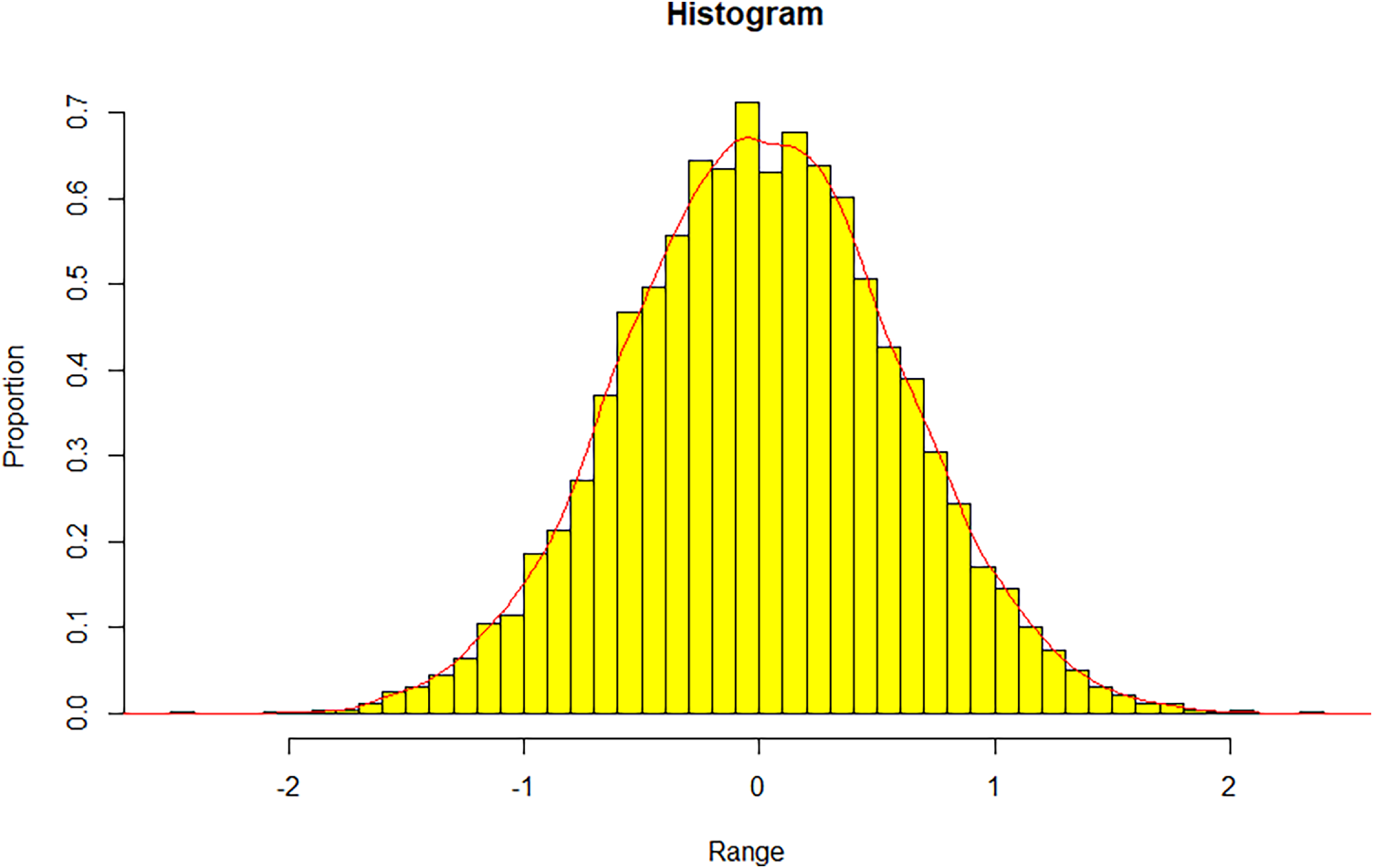


 Open access