





1. Introduction
In high-speed flows the interaction between shock waves and the boundary layer is a common phenomenon. This interaction, referred to in the literature as a shock wave/boundary layer interaction (SBLI), can have significant effects on aerothermodynamic loads and performance during high-speed flight and gas turbine operation. In the case of transonic airfoils, the occurrence of self-sustained shock wave oscillations, known as the buffet phenomenon (Lee Reference Lee2001), adds further complexity.
For these reasons, SBLIs have been one of the most important topics of research within the aeronautical scientific community over the past 70 years (Dolling Reference Dolling2001). Among others, Délery et al. (Reference Délery, Marvin and Reshotko1986), Smits & Dussauge (Reference Smits and Dussauge2006), Doerffer et al. (Reference Doerffer, Hirsch, Dussauge, Babinsky and Barakos2010) and Babinsky & Harvey (Reference Babinsky and Harvey2011) represent the most notable reviews on this topic. Incident normal shock, oblique shock reflection, compression ramps and transonic airfoils were, and still are nowadays, typical geometries employed to explore this phenomenon.
Dolling (Reference Dolling2001) reports that until the 1950s, SBLIs were commonly described as relatively steady. Nowadays, it is now known that this description is incorrect, at least for separated turbulent interactions. Quantitative measurements of turbulent SBLIs reported a low-frequency unsteadiness of the separation shock (Dolling & Murphy Reference Dolling and Murphy1983; Erengil & Dolling Reference Erengil and Dolling1991; Thomas, Putnam & Chu Reference Thomas, Putnam and Chu1994). The two orders of magnitude separating the characteristic frequency of the incoming boundary layer from the frequency of the separation shock explain why the unsteadiness is classified as being low frequency, relative to the higher characteristic frequency of the incoming turbulent boundary layer. The work of Dupont, Haddad & Debiève (Reference Dupont, Haddad and Debiève2006) noted that the rear part of the interaction for an oblique reflected shock geometry also exhibits unsteadiness, which is in quasi-linear dependence with the reflected shock motion. The low-frequency motion of the head shock, coupled to the expansion and contraction of the separated flow, is referred to as a breathing motion.
Whether discussing low-frequency unsteadiness or breathing motion, the necessity to find a consensus on the magnitude of the low-frequency oscillations prompted a search for temporal scaling. Erengil & Dolling (Reference Erengil and Dolling1991) used the interaction length $L_{int}$
, defined as the distance between the average position of the reflected shock and the extrapolation to the wall of the incident shock, and the upstream velocity
$L_{int}$
, defined as the distance between the average position of the reflected shock and the extrapolation to the wall of the incident shock, and the upstream velocity $U_{\infty }$
to scale the low-frequency unsteadiness. Based on this scaling, it was found in different experiments (Dupont et al. Reference Dupont, Haddad and Debiève2006; Dussauge, Dupont & Debiève Reference Dussauge, Dupont and Debiève2006; Ganapathisubramani, Clemens & Dolling Reference Ganapathisubramani, Clemens and Dolling2009; Piponniau et al. Reference Piponniau, Dussauge, Debieve and Dupont2009; Souverein et al. Reference Souverein, Van Oudheusden, Scarano and Dupont2009) and numerical investigations (Pirozzoli & Grasso Reference Pirozzoli and Grasso2006; Wu & Martin Reference Wu and Martin2008; Touber & Sandham Reference Touber and Sandham2009; Priebe & Martín Reference Priebe and Martín2012) that the low-frequency oscillations in turbulent SBLIs falls in the range of the Strouhal number
$U_{\infty }$
to scale the low-frequency unsteadiness. Based on this scaling, it was found in different experiments (Dupont et al. Reference Dupont, Haddad and Debiève2006; Dussauge, Dupont & Debiève Reference Dussauge, Dupont and Debiève2006; Ganapathisubramani, Clemens & Dolling Reference Ganapathisubramani, Clemens and Dolling2009; Piponniau et al. Reference Piponniau, Dussauge, Debieve and Dupont2009; Souverein et al. Reference Souverein, Van Oudheusden, Scarano and Dupont2009) and numerical investigations (Pirozzoli & Grasso Reference Pirozzoli and Grasso2006; Wu & Martin Reference Wu and Martin2008; Touber & Sandham Reference Touber and Sandham2009; Priebe & Martín Reference Priebe and Martín2012) that the low-frequency oscillations in turbulent SBLIs falls in the range of the Strouhal number $St = fL/U_{\infty } = 0.02{-}0.07$
, where
$St = fL/U_{\infty } = 0.02{-}0.07$
, where $f$
is the frequency associated with the low-frequency motion and
$f$
is the frequency associated with the low-frequency motion and $L$
and
$L$
and $U_{\infty }$
are as defined above. While the spatial and temporal dynamics of the global organisation of the flow have been illustrated (Dupont et al. Reference Dupont, Haddad and Debiève2006), and there is a clear comprehension of the qualitative mean flow organisation (Agostini et al. Reference Agostini, Larchevêque, Dupont, Debiève and Dussauge2012), several mechanisms, sometimes conflicting, have been proposed to describe the mechanisms that govern the turbulent unsteady interaction.
$U_{\infty }$
are as defined above. While the spatial and temporal dynamics of the global organisation of the flow have been illustrated (Dupont et al. Reference Dupont, Haddad and Debiève2006), and there is a clear comprehension of the qualitative mean flow organisation (Agostini et al. Reference Agostini, Larchevêque, Dupont, Debiève and Dussauge2012), several mechanisms, sometimes conflicting, have been proposed to describe the mechanisms that govern the turbulent unsteady interaction.
The unsteadiness of reflected shocks has been commonly linked to turbulent structures within the incoming boundary layer (Erengil Reference Erengil1993). Early studies by Uenalmis & Dolling (Reference Uenalmis and Dolling1994) identified a connection between small-scale shock motions and turbulence fluctuations or velocity fluctuations in the boundary layer. Ganapathisubramani, Clemens & Dolling (Reference Ganapathisubramani, Clemens and Dolling2007) later identified large-scale coherent structures, or superstructures, in the upstream boundary layer as responsible for low-frequency shock motion. Numerical simulations by Wu & Martin (Reference Wu and Martin2008) provided further insights, showing that the low-momentum structures of the incoming boundary layer and the separation point have a small correlation, indicating that the influence of the superstructures may be minimal. Additionally, it was found that both the shock motion and the motion of the separation point are correlated with the motion of the reattachment point, suggesting that the downstream flow contributes to the low-frequency unsteadiness. Further research has indicated a potential role for downstream mechanisms. Touber & Sandham (Reference Touber and Sandham2009) observed low-frequency unsteadiness even without upstream coherent structures, while Priebe et al. (Reference Priebe, Tu, Rowley and Martín2016) linked shock motion to downstream Görtler-like vortices. Another line of research has focused on the role of vortical structures emerging from the shear layer. Dussauge et al. (Reference Dussauge, Dupont and Debiève2006) suggested that the source of excitation of the shock motion can be attributed to eddies in the separated zone. Pirozzoli & Grasso (Reference Pirozzoli and Grasso2006) found that eddies in the separated zone interact with the shock, producing acoustic waves that propagate upstream and induce a low-frequency oscillation in the shock, reminiscent of acoustic resonance seen in cavity flows. Piponniau et al. (Reference Piponniau, Dussauge, Debieve and Dupont2009) proposed a model that relates the mass recharge within the separated bubble to the flapping dynamics occurring near the reattachment point. The main parameter controlling the low-frequency shock motions is the spreading rate of the compressible mixing layer. Recent works, such as Chandola & Estruch-Samper (Reference Chandola, Huang and Estruch-Samper2017) and Jenquin & Narayanaswamy (Reference Jenquin, Johnson and Narayanaswamy2023), support the role of mass imbalance within the separated bubble, driven by shear layer entrainment, as the driving mechanism for the pulsation of the separated bubble. A more recent consensus suggests that both upstream and internal mechanisms contribute to low-frequency unsteadiness. The work of Puckett & Narayanaswamy (Reference Puckett and Narayanaswamy2024) suggests that the combined effects of the separation bubbles inherent unsteadiness and the shear layer instabilities are key contributors to the dynamics of swept SBLIs. Thomas et al. (Reference Thomas, Putnam and Chu1994) and Dupont et al. (Reference Dupont, Haddad and Debiève2006) observed strong coherence in pressure fluctuations near the separation bubble and reattachment point, indicative of a ‘breathing’ mode of the separated region. Touber & Sandham (Reference Touber and Sandham2011) extended this understanding by demonstrating that the interaction between the shock and boundary layer could be modelled as a first-order low-pass filter, implying that the low-frequency unsteadiness is an intrinsic property of the system. Clemens & Narayanaswamy (Reference Clemens and Narayanaswamy2014) proposed that while both upstream and internal mechanisms are always present, downstream effects dominate in strongly separated flows, with a combined mechanism prevailing in weaker separations.
It is evident that the focus of researchers has largely centred on turbulent interactions, with only recent efforts directed towards studying laminar and transitional SBLIs. Robinet (Reference Robinet2007) conducted one of the earliest studies examining the temporal dynamics of laminar SBLIs. In his work, both three-dimensional (3-D) direct numerical simulations (DNS) and linearised global stability analysis were carried out on an incident oblique shock impinging onto a laminar boundary layer. Simulations highlighted that for an increasing angle of the incident shock, the flow becomes three dimensional, and the stability analysis revealed a bifurcation, generating the 3-D character of the flow. It was concluded that, beyond a critical angle of the incident shock wave, the two-dimensional (2-D) and stationary flow becomes linearly globally unstable to a 3-D stationary mode. However, Guiho, Alizard & Robinet (Reference Guiho, Alizard and Robinet2016) conducted a global stability analysis on a similar laminar interaction and found that the SBLI is globally stable for a wide range of flow parameters. They showed that unsteadiness is instead associated with nonlinear mechanisms between convective instabilities arising from the shear layer. The very recent study of Niessen et al. (Reference Niessen, Groot, Hickel and Terrapon2023) confirmed that the laminar SBLI they investigated cannot support the temporal growth of a disturbance in a fixed region of the space. Consequently, no 2-D global instabilities exist and, thus, all 2-D instability mechanisms are convective. They determined the most amplified perturbation content of a SBLI in terms of the most amplified spanwise wavelength, which was found to be as large as $10\,\%$
of the separated region, and frequency, about
$10\,\%$
of the separated region, and frequency, about $9\,{\textrm {kHz}}$
at the reattachment location. From these studies, it is clear that the low-frequency unsteadiness cannot be related to any unstable global mode.
$9\,{\textrm {kHz}}$
at the reattachment location. From these studies, it is clear that the low-frequency unsteadiness cannot be related to any unstable global mode.
Between the years $2012$
and
$2012$
and $2016$
, the European TFAST (transitional location effect on SBLI) project promoted several numerical simulations and experimental campaigns focused on transitional SBLIs. This project permitted progress in understanding the role of transition in the context of the mutual interaction between the shock system and the laminar boundary layer. In particular, the DNS work of Sansica, Sandham & Hu (Reference Sansica, Sandham and Hu2014) studied the global response of the separated region to white noise forcing both upstream and inside the bubble. It was concluded that the internal forcing causes the low-frequency response near the separation point. This result is in agreement with Guiho et al. (Reference Guiho, Alizard and Robinet2016), who showed that the low-frequency response at the separation is more effective when the forcing comes from the recirculating region than when forcing the upstream boundary layer. Bugeat et al. (Reference Bugeat, Robinet, Chassaing and Sagaut2022) suggested that the low-frequency dynamics of the SBLI corresponds to a forced damped stable mode, in which background perturbations through the receptivity mechanism continuously excite the flow. The flow thus behaves like a low-pass filter with respect to external disturbances.
$2016$
, the European TFAST (transitional location effect on SBLI) project promoted several numerical simulations and experimental campaigns focused on transitional SBLIs. This project permitted progress in understanding the role of transition in the context of the mutual interaction between the shock system and the laminar boundary layer. In particular, the DNS work of Sansica, Sandham & Hu (Reference Sansica, Sandham and Hu2014) studied the global response of the separated region to white noise forcing both upstream and inside the bubble. It was concluded that the internal forcing causes the low-frequency response near the separation point. This result is in agreement with Guiho et al. (Reference Guiho, Alizard and Robinet2016), who showed that the low-frequency response at the separation is more effective when the forcing comes from the recirculating region than when forcing the upstream boundary layer. Bugeat et al. (Reference Bugeat, Robinet, Chassaing and Sagaut2022) suggested that the low-frequency dynamics of the SBLI corresponds to a forced damped stable mode, in which background perturbations through the receptivity mechanism continuously excite the flow. The flow thus behaves like a low-pass filter with respect to external disturbances.
To study the mechanism in more detail, Sansica, Sandham & Hu (Reference Sansica, Sandham and Hu2016) forced the inlet of the interaction with a pair of monochromatic oblique unstable modes. Despite the clean upstream condition, they observed low-frequency unsteadiness near the separation point, with $St = 0.04$
. They attributed the appearance of unsteadiness to the breakdown of the deterministic turbulence, leading to broadband pressure disturbances travelling upstream through the separated region (within the subsonic layer of the boundary layer) at a phase velocity of
$St = 0.04$
. They attributed the appearance of unsteadiness to the breakdown of the deterministic turbulence, leading to broadband pressure disturbances travelling upstream through the separated region (within the subsonic layer of the boundary layer) at a phase velocity of $- 0.6 U_{\infty }$
. The acoustic nature of the backward travelling pressure waves was challenged by Larchevêque (Reference Larchevêque2016). In his study, fluidic backwards motion, with a possible origin at reattachment, was observed and the corresponding phase velocity, associated with low frequencies, was found to be
$- 0.6 U_{\infty }$
. The acoustic nature of the backward travelling pressure waves was challenged by Larchevêque (Reference Larchevêque2016). In his study, fluidic backwards motion, with a possible origin at reattachment, was observed and the corresponding phase velocity, associated with low frequencies, was found to be $- 0.22 U_{\infty }$
. Bonne et al. (Reference Bonne, Brion, Garnier, Bur, Molton, Sipp and Jacquin2019) conducted Reynolds-averaged Navier–Stokes-based simulations coupled with a resolvent analysis and confirmed the backward motion of waves through the recirculating region. However, they suggested a density or acoustic nature of those waves. Moreover, the low-frequency dynamics was described as a pseudo-resonance process that amplifies the instabilities in the separated shear layer and excites the shock foot, leading to the backward motion of density waves, with a phase velocity of
$- 0.22 U_{\infty }$
. Bonne et al. (Reference Bonne, Brion, Garnier, Bur, Molton, Sipp and Jacquin2019) conducted Reynolds-averaged Navier–Stokes-based simulations coupled with a resolvent analysis and confirmed the backward motion of waves through the recirculating region. However, they suggested a density or acoustic nature of those waves. Moreover, the low-frequency dynamics was described as a pseudo-resonance process that amplifies the instabilities in the separated shear layer and excites the shock foot, leading to the backward motion of density waves, with a phase velocity of $- 0.1 U_{\infty }$
. A similar scenario of density disturbances propagating upstream through the recirculating region with a group velocity of
$- 0.1 U_{\infty }$
. A similar scenario of density disturbances propagating upstream through the recirculating region with a group velocity of $- 0.18 U_{\infty }$
was observed experimentally by Threadgill, Little & Wernz (Reference Threadgill, Little and Wernz2021). Their detailed phase analysis of schlieren data permitted the identification of slow-moving density disturbances within the bubble that convect toward the shock foot and lead to the slow motion of the separation shock. Indeed, high-speed schlieren images showed that the separation shock exhibits low-frequency unsteadiness at
$- 0.18 U_{\infty }$
was observed experimentally by Threadgill, Little & Wernz (Reference Threadgill, Little and Wernz2021). Their detailed phase analysis of schlieren data permitted the identification of slow-moving density disturbances within the bubble that convect toward the shock foot and lead to the slow motion of the separation shock. Indeed, high-speed schlieren images showed that the separation shock exhibits low-frequency unsteadiness at $St = 0.025$
. To the current authors’ knowledge, this Strouhal value associated with the slow dynamics is the only one, in the context of the experiment, that is similar to those reported by numerical simulations.
$St = 0.025$
. To the current authors’ knowledge, this Strouhal value associated with the slow dynamics is the only one, in the context of the experiment, that is similar to those reported by numerical simulations.
Recent studies have suggested a nonlinear mechanism as a possible explanation for the low-frequency unsteadiness. Sansica et al. (Reference Sansica, Sandham and Hu2014) noted that low-frequency unsteadiness occurs even without direct low-frequency forcing, and it is due to weak nonlinear interactions with the shear layer instability modes. Mauriello, Larchevêque & Dupont (Reference Mauriello, Larchevêque and Dupont2022) suggest that quadratic couplings between oblique modes are responsible for the oscillation of the reflected shock. The low-frequency range in the separated region was found to be significantly quadratically coupled to the oblique mixing layer modes of much higher frequencies. They extended the analysis in the wavenumber space and showed that the flow features beneath the reflected shock, sustaining the low-frequency motion, are two dimensional. They also confirmed the existence of a slow upstream convective fluidic motion originating from the vicinity of the reattachment point. In their work, broadband and stochastic forcing was applied to stimulate the transition of the boundary layer to a turbulent state. Despite the non-forced transitional SBLI studied by Saïdi et al. (Reference Saïdi, Wang, Fournier, Tenaud and Robinet2025), similar strong triadic interactions were observed in the downstream region of the shock interaction playing a role in the low-frequency dynamics. However, in all these studies the nature of the nonlinearities that drives the unsteadiness remains unclear.
Building upon this body of work, the present work aims to investigate the presence of any unsteadiness and to address fundamental questions about the nature of nonlinearities in the context of the transitional SBLI. Motivated by the distinct approaches employed in prior research, wherein Mauriello et al.’s (Reference Mauriello, Larchevêque and Dupont2022) work incorporated broadband forcing and Saïdi et al.’s (Reference Saïdi, Wang, Fournier, Tenaud and Robinet2025) study focused on a non-forced SBLI, the decision was to construct a simplified and didactic model. This model was designed to include a modal transition and enable precise control of the input parameters. Accordingly, one-period DNS combined with high-order statistical analysis have been performed on a $M= 1.5$
oblique shock reflection with separation. All details of the numerical set-up and the flow conditions are given in § 2. Starting from the work of Sansica et al. (Reference Sansica, Sandham and Hu2016), which suggests that the origin of the low-frequency unsteadiness is due to the breakdown into turbulence, deterministic simulations have been performed. The deterministic approach allows full control of the input conditions. We first reproduced the basic configuration used in the work of Sansica et al. (Reference Sansica, Sandham and Hu2016), where the incoming laminar boundary layer is stimulated with a pair of monochromatic oblique unstable modes. The result, presented in § 3, showed that a pair of oblique unstable modes is not sufficient to produce the low-frequency response of the head shock, although the breakdown to turbulence is observed to persist. Consequently, we have combined two different (in frequency) and opposite (in wavenumber) arrangements of unstable boundary layer modes. Our aim is to see if the introduction of nonlinearities triggers both the low-frequency unsteadiness and the transition to turbulence in the boundary layer. Results are presented in § 4. This deterministic approach, while providing valuable insights into the fundamental nonlinear interactions, inherently presents certain limitations. The use of specific monochromatic forcing arrangements represents a simplification of the broadband disturbances present in natural flows. Despite these limitations, this work addressed fundamental questions regarding the nature of nonlinearities driving low-frequency unsteadiness. In § 5 we are interested in studying potential triadic interactions between the structures responsible for the boundary layer transition and those arising at the separation point. To achieve this, we have used high-order statistical tools. High-order spectral analysis is also used to identify the signature of low-frequency unsteadiness in wavenumber space. Two additional forcing configurations and a case with a different frequency combination are presented in § 6. The concluding § 7 summarises all the outcomes of this study.
$M= 1.5$
oblique shock reflection with separation. All details of the numerical set-up and the flow conditions are given in § 2. Starting from the work of Sansica et al. (Reference Sansica, Sandham and Hu2016), which suggests that the origin of the low-frequency unsteadiness is due to the breakdown into turbulence, deterministic simulations have been performed. The deterministic approach allows full control of the input conditions. We first reproduced the basic configuration used in the work of Sansica et al. (Reference Sansica, Sandham and Hu2016), where the incoming laminar boundary layer is stimulated with a pair of monochromatic oblique unstable modes. The result, presented in § 3, showed that a pair of oblique unstable modes is not sufficient to produce the low-frequency response of the head shock, although the breakdown to turbulence is observed to persist. Consequently, we have combined two different (in frequency) and opposite (in wavenumber) arrangements of unstable boundary layer modes. Our aim is to see if the introduction of nonlinearities triggers both the low-frequency unsteadiness and the transition to turbulence in the boundary layer. Results are presented in § 4. This deterministic approach, while providing valuable insights into the fundamental nonlinear interactions, inherently presents certain limitations. The use of specific monochromatic forcing arrangements represents a simplification of the broadband disturbances present in natural flows. Despite these limitations, this work addressed fundamental questions regarding the nature of nonlinearities driving low-frequency unsteadiness. In § 5 we are interested in studying potential triadic interactions between the structures responsible for the boundary layer transition and those arising at the separation point. To achieve this, we have used high-order statistical tools. High-order spectral analysis is also used to identify the signature of low-frequency unsteadiness in wavenumber space. Two additional forcing configurations and a case with a different frequency combination are presented in § 6. The concluding § 7 summarises all the outcomes of this study.
It is essential to emphasise that this study focuses specifically on transitional SBLIs. Relating the observed phenomena directly to turbulent SBLIs is challenging due to the fundamental differences in their spectral content and nature of the flows. Moreover, the deterministic approach allows for precise control and analysis of nonlinear interactions, but it also limits the direct extension to fully turbulent scenarios.
2. Flow conditions and numerical set-up
2.1. Numerical method and flow conditions
The 3-D compressible Navier–Stokes equations are solved in the conservative form, and are presented in the Cartesian coordinate system as
 \begin{align} \frac {\partial \rho }{\partial t} + \frac {\partial \rho u_{j}}{\partial x_{j}} = 0, \\[-30pt]\nonumber\end{align}
 \begin{align} \frac {\partial \rho u_{i}}{\partial t} +\frac {\partial \rho u_{i} u_{j}}{\partial x_{j}} = - \frac {\partial p}{\partial x_{i}} + \frac {1}{Re}\frac {\partial \tau _{ij}}{\partial x_{j}} ,\\[-30pt]\nonumber\end{align}
 \begin{align} \frac {\partial \rho E}{\partial t} + \frac {\partial (\rho E + p) u_{j}}{\partial x_{j}} = \frac {1}{(\gamma -1)Re Pr M_{\infty }^2}\frac {\partial }{\partial x_{j}}\left (\mu \frac {\partial T}{\partial x_{j}}\right ) + \frac {1}{Re}\frac {\partial \tau _{ij}u_{i}}{\partial x_{j}}, \end{align}
showing the non-dimensional form of the mass conservation equation, three momentum conservation equations and the energy conservation equation, respectively. The indices $i$
and
$i$
and $j$
run from 1 to 3. In the equations,
$j$
run from 1 to 3. In the equations, $\rho = \rho ^*/\rho _\infty ^*$
is the non-dimensional density,
$\rho = \rho ^*/\rho _\infty ^*$
is the non-dimensional density, $u_1=u=u^*/U_\infty ^*$
,
$u_1=u=u^*/U_\infty ^*$
, $u_2=v=v^*/U_\infty ^*$
and
$u_2=v=v^*/U_\infty ^*$
and $u_3=w=w^*/U_\infty ^*$
are the non-dimensional velocity components respectively in the
$u_3=w=w^*/U_\infty ^*$
are the non-dimensional velocity components respectively in the $x$
,
$x$
, $y$
and
$y$
and $z$
directions scaled with free-stream velocity
$z$
directions scaled with free-stream velocity $U_\infty ^*$
;
$U_\infty ^*$
; $E = e + 1/2 \rho (u^2+v^2+w^2)$
is the total energy per unit mass, with
$E = e + 1/2 \rho (u^2+v^2+w^2)$
is the total energy per unit mass, with $e$
as specific internal energy. The corresponding conservative variables are
$e$
as specific internal energy. The corresponding conservative variables are $\rho$
,
$\rho$
, $\rho u$
,
$\rho u$
, $\rho v$
,
$\rho v$
, $\rho w$
and
$\rho w$
and $\rho E$
. The terms
$\rho E$
. The terms $p$
,
$p$
, $T$
are the non-dimensional pressure and temperature, respectively, while
$T$
are the non-dimensional pressure and temperature, respectively, while $\tau _{ij} = \mu [ \partial u_{i}/\partial x_j + \partial u_{j}/\partial x_i -2/3 (\partial u_{k}/\partial x_k) \delta _{ij} ]$
is the viscous stress tensor, where
$\tau _{ij} = \mu [ \partial u_{i}/\partial x_j + \partial u_{j}/\partial x_i -2/3 (\partial u_{k}/\partial x_k) \delta _{ij} ]$
is the viscous stress tensor, where $\mu$
is the non-dimensional dynamic viscosity given by Sutherland’s law, with a Sutherland temperature of
$\mu$
is the non-dimensional dynamic viscosity given by Sutherland’s law, with a Sutherland temperature of $T_S^*=110.4\,{\textrm {K}}$
, and
$T_S^*=110.4\,{\textrm {K}}$
, and $\delta _{ij}$
is the Kronecker delta function. The various physical variables are normalised using the corresponding free-stream values. However, pressure is normalised using the free-stream dynamic pressure term,
$\delta _{ij}$
is the Kronecker delta function. The various physical variables are normalised using the corresponding free-stream values. However, pressure is normalised using the free-stream dynamic pressure term, $\rho _\infty ^{*} U_\infty ^{*2}$
, i.e.
$\rho _\infty ^{*} U_\infty ^{*2}$
, i.e. $p = p^*/\rho _\infty ^{*} U_\infty ^{*2}$
, while the unit total energy
$p = p^*/\rho _\infty ^{*} U_\infty ^{*2}$
, while the unit total energy $E$
is normalised by
$E$
is normalised by $ U_\infty ^{*2}$
. The dimensional quantities are denoted by a superscript
$ U_\infty ^{*2}$
. The dimensional quantities are denoted by a superscript $ ^{*}$
, which is dropped for non-dimensional quantities unless mentioned otherwise. Also, the subscript `
$ ^{*}$
, which is dropped for non-dimensional quantities unless mentioned otherwise. Also, the subscript ` $_{\infty }$
’ represents the free-stream conditions at the inflow. Here
$_{\infty }$
’ represents the free-stream conditions at the inflow. Here $x=x^*/\delta _{\textit{inlet}}^{*}$
,
$x=x^*/\delta _{\textit{inlet}}^{*}$
, $y=y^*/\delta _{\textit{inlet}}^{*}$
and
$y=y^*/\delta _{\textit{inlet}}^{*}$
and $z=z^*/\delta _{\textit{inlet}}^{*}$
are the non-dimensional coordinates scaled with the displacement thickness
$z=z^*/\delta _{\textit{inlet}}^{*}$
are the non-dimensional coordinates scaled with the displacement thickness $\delta _{\textit{inlet}}^{*}=0.075$
(mm) at the inflow. The characteristic fluid dynamic time scale is
$\delta _{\textit{inlet}}^{*}=0.075$
(mm) at the inflow. The characteristic fluid dynamic time scale is $\delta _{\textit{inlet}}^{*}/U_\infty ^*$
.
$\delta _{\textit{inlet}}^{*}/U_\infty ^*$
.
The OpenSBLI solver (Lusher, Jammy & Sandham Reference Lusher, Jammy and Sandham2021), which is an open-source finite-difference-based solver, is used on structured Cartesian coordinate systems for the shock-reflection set-up. A local Lax--Friedrichs flux splitting approach is used for the inviscid fluxes in characteristic space. Different variations of flux reconstruction schemes, i.e. weighted essentially non-oscillatory (WENO) and targeted essentially non-oscillatory (TENO), are available to compute the inviscid fluxes. As noted in earlier literature, the TENO scheme is less dissipative than the WENO schemes and, hence, an adaptive version of sixtth-order TENO is used to perform the present simulations (Lusher et al. Reference Lusher, Jammy and Sandham2021). The viscous fluxes are computed using fourth-order central differences, while a third-order Runge–Kutta scheme is used for time integration.
Two-dimensional schematic of the numerical set-up, where the computational domain is demarcated with a red dashed line.

A 2-D schematic of the computational set-up is shown in figure 1. The computational domain, marked with a red dashed line, has extents $0 \leqslant x \leqslant 375$
,
$0 \leqslant x \leqslant 375$
, $0 \leqslant y \leqslant 140$
,
$0 \leqslant y \leqslant 140$
, $0 \leqslant z \leqslant 27.32$
, and the number of points (
$0 \leqslant z \leqslant 27.32$
, and the number of points ( $N_x$
,
$N_x$
, $N_y$
,
$N_y$
, $N_z$
) = (2050, 325, 200). The origin is located at the beginning of the computational domain. The grids are stretched in the wall-normal (
$N_z$
) = (2050, 325, 200). The origin is located at the beginning of the computational domain. The grids are stretched in the wall-normal ( $y$
) direction using a tangent hyperbolic stretching function, while the grids are uniform in both streamwise (
$y$
) direction using a tangent hyperbolic stretching function, while the grids are uniform in both streamwise ( $x$
) and spanwise (
$x$
) and spanwise ( $z$
) directions. All the distances are scaled with the displacement thickness
$z$
) directions. All the distances are scaled with the displacement thickness $\delta _{\textit{inlet}}^{*}=0.075$
(mm) at the inflow plane, which is initialised using a similarity solution for a Mach 1.5 flow with a unit Reynolds number of
$\delta _{\textit{inlet}}^{*}=0.075$
(mm) at the inflow plane, which is initialised using a similarity solution for a Mach 1.5 flow with a unit Reynolds number of $10^{7}$
(m−1). Hence, the simulation Reynolds number based on this
$10^{7}$
(m−1). Hence, the simulation Reynolds number based on this $\delta _{\textit{inlet}}^{*}$
is
$\delta _{\textit{inlet}}^{*}$
is $Re=750$
.
$Re=750$
.
The reference conditions are the same as Sansica et al. (Reference Sansica, Sandham and Hu2016), and table 1 summarises the aerodynamic parameters. At the wall, no-slip and isothermal boundary conditions (where the wall temperature is set to the laminar adiabatic wall temperature, i.e. $T_{\textit{wall}} = T^*_{\textit{wall}}/T^*_{\infty } \approx 1.381$
) are used. Here, the reference free-stream temperature is
$T_{\textit{wall}} = T^*_{\textit{wall}}/T^*_{\infty } \approx 1.381$
) are used. Here, the reference free-stream temperature is $T^*_{\infty } = 202.17$
K. An extrapolation method is used at the inflow (for pressure) and outflow, while the span is periodic. The top boundary has shock jump conditions for a wedge angle of 2.5
$T^*_{\infty } = 202.17$
K. An extrapolation method is used at the inflow (for pressure) and outflow, while the span is periodic. The top boundary has shock jump conditions for a wedge angle of 2.5 $^{\circ }$
at
$^{\circ }$
at $x=20$
, resulting in a pressure rise of
$x=20$
, resulting in a pressure rise of $p_{3}/p_{1}= 1.28$
, where
$p_{3}/p_{1}= 1.28$
, where $p_{3}$
indicates the pressure state after the reflected shock. The Reynolds number at the location of inviscid shock impingement from the leading edge of the flat plate is
$p_{3}$
indicates the pressure state after the reflected shock. The Reynolds number at the location of inviscid shock impingement from the leading edge of the flat plate is $Re_{\tilde {x}_{imp}} = 1.95 \times 10^{5}$
. These are further depicted in the schematic of the domain in figure 1.
$Re_{\tilde {x}_{imp}} = 1.95 \times 10^{5}$
. These are further depicted in the schematic of the domain in figure 1.
Aerodynamic flow conditions.

Disturbances are applied, upstream of the separation bubble, as a body-forcing term in the continuity equation, and a sample oblique wave representation with a particular frequency and spanwise wavenumber is given as
 \begin{equation} {\rho '}(x,y,z,t) = {\textrm {Real}} \left[A_0 \exp \left[- (x-x_c)^2 - (y-y_c)^2\right]{\exp} \big[i(\pm \beta z - \omega t)\big]\right], \end{equation}
where $A_0$
represents the amplitude of the forcing, while (
$A_0$
represents the amplitude of the forcing, while ( $x_c$
,
$x_c$
, $y_c$
) = (20, 4) are the coordinates where the forcing is centred, which is roughly located at the edge of the shear layer. The forcing takes a maximum value at the central location and then tapers off in both
$y_c$
) = (20, 4) are the coordinates where the forcing is centred, which is roughly located at the edge of the shear layer. The forcing takes a maximum value at the central location and then tapers off in both $x$
and
$x$
and $y$
directions due to the first exponential term in (2.4). The last exponential term introduces variation in the spanwise and temporal dimensions, representing an oblique wave that travels at different angles with respect to the
$y$
directions due to the first exponential term in (2.4). The last exponential term introduces variation in the spanwise and temporal dimensions, representing an oblique wave that travels at different angles with respect to the $z$
direction depending upon the + or − sign. The values of the spanwise wavenumber and circular frequency (
$z$
direction depending upon the + or − sign. The values of the spanwise wavenumber and circular frequency ( $\beta$
and
$\beta$
and $\omega$
, respectively) are obtained from the linear stability theory (Sansica et al. Reference Sansica, Sandham and Hu2016).
$\omega$
, respectively) are obtained from the linear stability theory (Sansica et al. Reference Sansica, Sandham and Hu2016).
Various combinations of the simple deterministic forcing represented by (2.4) are used to trigger flow transition, the simplest of which is a pair of oblique waves with single circular frequency as used in Sansica et al. (Reference Sansica, Sandham and Hu2016). As the modifications represent a key point in this study, an entire section (see § 4) has been devoted to a comprehensive and detailed treatment of them. At this point in the text it is important to emphasise that, when two frequencies are forced, the combination is designed to be periodic over one cycle of the difference frequency (i.e. $T=2\pi /\Delta \omega$
). This periodicity should be evident in the response flow field under these forcings, and once this was ensured, the wall pressure data was collected over one cycle of this difference frequency to evaluate the frequency spectrum.
$T=2\pi /\Delta \omega$
). This periodicity should be evident in the response flow field under these forcings, and once this was ensured, the wall pressure data was collected over one cycle of this difference frequency to evaluate the frequency spectrum.
2.2. High-order analysis
High-order spectra, corresponding to the Fourier transform of high-order correlation functions, are the preferred tools to study nonlinear interactions since they allow the analysis of the quadratic couplings present in the governing Navier–Stokes equations on a scale-by-scale basis.
One relevant high-order spectrum is the bispectrum (Tynan et al. Reference Tynan, Moyer, Burin and Holland2001). It is formally defined as the Fourier transform of the triple correlation, given by
 \begin{equation} {\textit{Bis}}_{\textit{FGH}}\!\left (\boldsymbol{x_F},\boldsymbol{x_G},\boldsymbol{x_H},f_1,f_2\right )= \langle \hat {F}\!\left (\boldsymbol{x_F},f_1\right )\, \hat {G}\!\left (\boldsymbol{x_G},f_2\right )\, \hat {H}^*\!\left (\boldsymbol{x_H},f_1+f_2\right ) \rangle , \end{equation}
where $\langle \rangle$
denotes the averaging operation over time segments and possibly the homogeneous direction. Here
$\langle \rangle$
denotes the averaging operation over time segments and possibly the homogeneous direction. Here $\hat {F}$
,
$\hat {F}$
, $\hat {G}$
and
$\hat {G}$
and $\hat {H}$
are the temporal Fourier transforms at the locations
$\hat {H}$
are the temporal Fourier transforms at the locations $\boldsymbol{x_{F}}, \boldsymbol{x_{G}}$
and
$\boldsymbol{x_{F}}, \boldsymbol{x_{G}}$
and $\boldsymbol{x_{H}}$
, and the superscript
$\boldsymbol{x_{H}}$
, and the superscript $^{*}$
indicates the complex conjugate. The bispectrum reveals the energy content associated with the cross-interaction between
$^{*}$
indicates the complex conjugate. The bispectrum reveals the energy content associated with the cross-interaction between $\hat {F}$
and
$\hat {F}$
and $\hat {G}$
(
$\hat {G}$
( $\hat {F} \times \hat {G}$
) and a third signal
$\hat {F} \times \hat {G}$
) and a third signal $\hat {H}$
at the frequency
$\hat {H}$
at the frequency $f_1+f_2$
. This tool has been used extensively in the work of Mauriello (Reference Mauriello2024), where a broadband stochastic forcing was used to stimulate the boundary layer transition in the case of a transition SBLI at Mach 1.7. It has been proven to be very powerful in highlighting the triadic interactions that occur between the oblique modes, i.e. the coherent structures responsible for the transition to the turbulent state of the boundary layer, and the structures of a 2-D nature that emerge at the separation point. In the present work, the modal transition has been fostered and a deterministic forcing has been applied (see § 4), plus the periodicity of the present simulations (one-period simulation) imposes that, for the lowest frequency
$f_1+f_2$
. This tool has been used extensively in the work of Mauriello (Reference Mauriello2024), where a broadband stochastic forcing was used to stimulate the boundary layer transition in the case of a transition SBLI at Mach 1.7. It has been proven to be very powerful in highlighting the triadic interactions that occur between the oblique modes, i.e. the coherent structures responsible for the transition to the turbulent state of the boundary layer, and the structures of a 2-D nature that emerge at the separation point. In the present work, the modal transition has been fostered and a deterministic forcing has been applied (see § 4), plus the periodicity of the present simulations (one-period simulation) imposes that, for the lowest frequency $f_{min} = 1/T$
, only a single segment, encompassing fully the period, can be considered. It therefore excludes the possibility of averaging over segments leading to a meaningless value of the normalised form of the bispectrum, i.e. the bicoherence (
$f_{min} = 1/T$
, only a single segment, encompassing fully the period, can be considered. It therefore excludes the possibility of averaging over segments leading to a meaningless value of the normalised form of the bispectrum, i.e. the bicoherence ( $Bic = 1$
). With this in mind, the bispectral analysis presented above is reformulated in terms of spanwise wavenumbers taking advantage of the time/space duality found for both the oblique mode and the low-frequency unsteadiness (Mauriello Reference Mauriello2024). This version of the bispectrum is given by
$Bic = 1$
). With this in mind, the bispectral analysis presented above is reformulated in terms of spanwise wavenumbers taking advantage of the time/space duality found for both the oblique mode and the low-frequency unsteadiness (Mauriello Reference Mauriello2024). This version of the bispectrum is given by
 \begin{align} &{\textit{Bis}}_{\textit{FGH}}\big(({x_F}, {y_F}),({x_G}, {y_G}),({x_H}, {y_H}),k_{z_{1}},k_{z_{2}}\big)\nonumber\\ &\quad=\langle \hat {F}\big(({x_F}, {y_F}),k_{z_{1}},t\big)\hat {G}\big(({x_G}, {y_G}),k_{z_{2}},t\big)\hat {H}^*\big(({x_H}, {y_H}),k_{z_{1}}+k_{z_{2}},t\big)\rangle, \end{align}
where $\langle \rangle$
denotes a time average over one period. In this way, it is possible to detect the wavenumbers responsible for nonlinear interactions among the fixed locations
$\langle \rangle$
denotes a time average over one period. In this way, it is possible to detect the wavenumbers responsible for nonlinear interactions among the fixed locations $({x_F}, {y_F}),({x_G}, {y_G}),({x_H}, {y_H})$
. By time averaging in the wavenumber space, information about the temporal behaviour is lost, but can be partially recovered by introducing a time delay
$({x_F}, {y_F}),({x_G}, {y_G}),({x_H}, {y_H})$
. By time averaging in the wavenumber space, information about the temporal behaviour is lost, but can be partially recovered by introducing a time delay $\tau$
. The time delay can be introduced for the two time series
$\tau$
. The time delay can be introduced for the two time series $F$
and
$F$
and $G$
, consequently
$G$
, consequently $\tau _{1}$
and
$\tau _{1}$
and $\tau _{2}$
identify the time lag occurring with respect to the third time series
$\tau _{2}$
identify the time lag occurring with respect to the third time series $H(f)$
. The formula can be written as
$H(f)$
. The formula can be written as
 \begin{align}&{\textit{Bis}}_{\textit{FGH}}\big(({x_F}, {y_F}),({x_G}, {y_G}),({x_H}, {y_H}),k_{z_{1}},k_{z_{2}}, \tau _{1}, \tau _{2} \big)\nonumber\\&\quad=\langle \hat {F}\big(({x_F}, {y_F}),k_{z_{1}}, t + \tau _{1}\big)\hat {G}\big(({x_G}, {y_G}),k_{z_{2}}, t + \tau _{2}\big)\,\hat {H}^*\big(({x_H}, {y_H}),k_{z_{1}}+k_{z_{2}}, t \big)\rangle,\end{align}
In addition to the standard bispectrum maps defined in (2.7), optimal bispectrum maps can be extracted. These maps are optimal in the sense that, for all possible time-delay pairs, the optimal time delay $\tau _{opt}$
is such that it maximises the bispectral energy content. For the sake of simplicity, the Fourier transforms
$\tau _{opt}$
is such that it maximises the bispectral energy content. For the sake of simplicity, the Fourier transforms $\hat {F}$
,
$\hat {F}$
, $\hat {G}$
and
$\hat {G}$
and $\hat {H}$
will all be referred to by the letter
$\hat {H}$
will all be referred to by the letter $G$
in the remainder of the text, and will be distinguished by subscript numbers running from 1 to 3.
$G$
in the remainder of the text, and will be distinguished by subscript numbers running from 1 to 3.
3. Reference case of transitional SBLI
Sansica (Reference Sansica2015) presented a detailed study using the local linear stability analysis, which identified the most unstable modes for the shock-reflection problem. Sansica et al. (Reference Sansica, Sandham and Hu2016) further performed DNS using these modes to perform the oblique mode transition using a pair of oblique modes to trigger transition. Lusher et al. (Reference Lusher, Jammy and Sandham2021) used the OpenSBLI solver to repeat these oblique mode transition simulations, however, with different numerical methods and forcing set-up. As we use the OpenSBLI solver in the present research, we wanted to first cross-validate our results against Lusher et al. (Reference Lusher, Jammy and Sandham2021), starting with oblique mode transition, before performing more complicated forcing combinations that are further explored in this study. We next explain the validation results in this section.
The modal forcing is applied as a prescribed time-dependent forcing, where the density disturbances $\rho '(x,y,z,t)$
are superimposed on the density laminar flow field at
$\rho '(x,y,z,t)$
are superimposed on the density laminar flow field at $(x_{c}, y_{c}) = (20,4)$
. The values of the streamwise and spanwise wavenumbers (
$(x_{c}, y_{c}) = (20,4)$
. The values of the streamwise and spanwise wavenumbers ( $\alpha$
and
$\alpha$
and $\beta$
, respectively) as well as the pulsation frequency
$\beta$
, respectively) as well as the pulsation frequency $\omega$
were extracted from the temporal stability map (see figure 4.3 of Sansica Reference Sansica2015). The spanwise width of the domain is set as
$\omega$
were extracted from the temporal stability map (see figure 4.3 of Sansica Reference Sansica2015). The spanwise width of the domain is set as $L_{z} = 2 \pi / \beta$
such that it accommodates at least one wavelength of the most unstable oblique mode. Hence, the decision to set
$L_{z} = 2 \pi / \beta$
such that it accommodates at least one wavelength of the most unstable oblique mode. Hence, the decision to set $L_{z} = 2 \pi / \beta = \lambda _{z} = 27.32$
.
$L_{z} = 2 \pi / \beta = \lambda _{z} = 27.32$
.
The first set of simulations, that are performed using the deterministic forcing approach, use a pair of monochromatic oblique unstable modes, as used in Sansica et al. (Reference Sansica, Sandham and Hu2016) and Lusher et al. (Reference Lusher, Jammy and Sandham2021), and the resultant forcing expression is given as
 \begin{equation} {\rho '}(x,y,z,t) = {\textrm {Real}}\left[A_{0}\,{\exp} \left[- (x-x_c)^2 - (y-y_c)^2\right]\left(e^{i( +\beta z - \omega t)} + e^{i( -\beta z - \omega t)}\right)\right]. \end{equation}
The oblique mode pair in the forcing expression uses $A_{0} = 1.25 \times 10^{-3}$
,
$A_{0} = 1.25 \times 10^{-3}$
, $\beta = 0.23$
and a single frequency value of
$\beta = 0.23$
and a single frequency value of $\omega =0.101$
, similar to Sansica et al. (Reference Sansica, Sandham and Hu2016), to force the separated boundary layer. The OpenSBLI solver is used to run these simulations and the set-up is identical to Lusher et al. (Reference Lusher, Jammy and Sandham2021), except that we used a uniform grid in the streamwise direction. The aerodynamic conditions used in Lusher et al. (Reference Lusher, Jammy and Sandham2021), including the free-stream and shock jump conditions and shock impingement location, are the same as Sansica et al. (Reference Sansica, Sandham and Hu2016). However, the present simulation is different from Sansica et al. (Reference Sansica, Sandham and Hu2016) due to the way the forcing is applied. In the current simulations, the forcing is applied as a volumetric forcing in the density term centred at
$\omega =0.101$
, similar to Sansica et al. (Reference Sansica, Sandham and Hu2016), to force the separated boundary layer. The OpenSBLI solver is used to run these simulations and the set-up is identical to Lusher et al. (Reference Lusher, Jammy and Sandham2021), except that we used a uniform grid in the streamwise direction. The aerodynamic conditions used in Lusher et al. (Reference Lusher, Jammy and Sandham2021), including the free-stream and shock jump conditions and shock impingement location, are the same as Sansica et al. (Reference Sansica, Sandham and Hu2016). However, the present simulation is different from Sansica et al. (Reference Sansica, Sandham and Hu2016) due to the way the forcing is applied. In the current simulations, the forcing is applied as a volumetric forcing in the density term centred at $(x_{c}, y_{c}) = (20,4)$
, i.e. downstream of the inlet plane and upstream of the separation bubble, while in Sansica et al. (Reference Sansica, Sandham and Hu2016) the forcing was applied at the inflow in terms of the eigenfunctions for all conservative variables.
$(x_{c}, y_{c}) = (20,4)$
, i.e. downstream of the inlet plane and upstream of the separation bubble, while in Sansica et al. (Reference Sansica, Sandham and Hu2016) the forcing was applied at the inflow in terms of the eigenfunctions for all conservative variables.
As we reran the set-up of Lusher et al. (Reference Lusher, Jammy and Sandham2021) with a uniform grid in the streamwise direction, we performed some initial verification of our results against the skin friction results extracted from the reference. Figure 2(a) shows a comparison of skin friction from the rerun of Lusher et al.’s (Reference Lusher, Jammy and Sandham2021) set-up with two different schemes, i.e. WENO and TENO. The 2-D laminar skin friction is also plotted for reference. It can be seen that the TENO version shows a slightly better agreement with Lusher et al. (Reference Lusher, Jammy and Sandham2021) compared with the WENO version. Some minor deviations are noted towards the exit of the domain perhaps due to streamwise stretching used in the reference simulation of Lusher et al. (Reference Lusher, Jammy and Sandham2021). Figure 2(b) shows minimal variations of non-dimensional wall pressure, which is further non-dimensionalised with the reference pressure $P_{\infty }=1/\gamma M_\infty ^2$
between the schemes. The 2-D laminar wall pressure is also shown as a reference.
$P_{\infty }=1/\gamma M_\infty ^2$
between the schemes. The 2-D laminar wall pressure is also shown as a reference.
Streamwise evolution of the friction coefficient $C_f$
(a) and of the pressure at the wall normalised with the reference pressure
$C_f$
(a) and of the pressure at the wall normalised with the reference pressure $P_{\textit{wall}}/P_{\infty }$
(b).
$P_{\textit{wall}}/P_{\infty }$
(b).

Three-dimensional view showing slices of $\rho u$
. The initial symmetry and its breakdown due to transition at downstream locations is shown.
$\rho u$
. The initial symmetry and its breakdown due to transition at downstream locations is shown.

A 3-D visualisation of the flow is shown in figure 3, which shows streamwise momentum $\rho u$
at equally spaced
$\rho u$
at equally spaced $x$
–
$x$
– $y$
plane slices, with the first slice placed close to the reattachment point at
$y$
plane slices, with the first slice placed close to the reattachment point at $x \approx 190$
. The second slice at
$x \approx 190$
. The second slice at $x\approx 230$
shows the first signs of spanwise non-uniformity due to the production of streamwise vorticity. The spanwise symmetry starts to break once further smaller scales are generated due to the transition to turbulence.
$x\approx 230$
shows the first signs of spanwise non-uniformity due to the production of streamwise vorticity. The spanwise symmetry starts to break once further smaller scales are generated due to the transition to turbulence.
Figure 4 shows the spectral content of the pressure fluctuations at the wall in an $x$
–
$x$
– $f$
plane, where
$f$
plane, where $x$
is the non-dimensional streamwise distance, shown in a linear scale, while
$x$
is the non-dimensional streamwise distance, shown in a linear scale, while $f$
is the non-dimensional frequency, shown with a logarithmic scale. The frequency is normalised using the reference frequency scale
$f$
is the non-dimensional frequency, shown with a logarithmic scale. The frequency is normalised using the reference frequency scale $U^{*}_{\infty }/\delta _{\textit{inlet}}^{*}$
. In this way, the
$U^{*}_{\infty }/\delta _{\textit{inlet}}^{*}$
. In this way, the $y$
axis gives the Strouhal number based on the length scale
$y$
axis gives the Strouhal number based on the length scale $\delta _{\textit{inlet}}^{*}$
. It is worth mentioning that, unless explicitly stated otherwise, the same normalisations (for
$\delta _{\textit{inlet}}^{*}$
. It is worth mentioning that, unless explicitly stated otherwise, the same normalisations (for $x$
and
$x$
and $f$
) will be applied to all the other spectra presented in this study. The spectrum clearly shows the forcing
$f$
) will be applied to all the other spectra presented in this study. The spectrum clearly shows the forcing $f=\omega /2\pi \approx 1.6 \times 10^{-2}$
introduced at
$f=\omega /2\pi \approx 1.6 \times 10^{-2}$
introduced at $x = 20$
. Its energy content extends over the whole domain and, starting from
$x = 20$
. Its energy content extends over the whole domain and, starting from $x=150$
, subsequent harmonics develop towards increasingly higher frequencies. This indicates that in the reattachment zone the boundary layer transitions to a turbulent state containing increasingly smaller structures (small scales) and increasingly higher frequencies. However, the separation point around
$x=150$
, subsequent harmonics develop towards increasingly higher frequencies. This indicates that in the reattachment zone the boundary layer transitions to a turbulent state containing increasingly smaller structures (small scales) and increasingly higher frequencies. However, the separation point around $x=110$
is free of any energy content, indicating that no low-frequency unsteadiness arises with this specific deterministic forcing.
$x=110$
is free of any energy content, indicating that no low-frequency unsteadiness arises with this specific deterministic forcing.
The present power spectrum differs in one respect from Sansica et al. (Reference Sansica, Sandham and Hu2016), where weak low-frequency unsteadiness was identified using a local (in $x$
) normalisation. Besides the difference in the normalisation, there are a few differences in methodology. In the current simulations, the perturbations are introduced as a body-forcing source term through the density equation downstream of the inflow plane, while in Sansica’s case the forcing was applied at the inlet through the entire state vector. Also, the numerical method used in Sansica’s case included a total variation diminishing scheme (Sansica Reference Sansica2015) for shock capturing, while the present study uses a TENO scheme. On the hypothesis that the low-frequency content of the baseline case is sensitive to the numerical noise level, we prefer in the next section to introduce the nonlinearities in a deterministic way.
$x$
) normalisation. Besides the difference in the normalisation, there are a few differences in methodology. In the current simulations, the perturbations are introduced as a body-forcing source term through the density equation downstream of the inflow plane, while in Sansica’s case the forcing was applied at the inlet through the entire state vector. Also, the numerical method used in Sansica’s case included a total variation diminishing scheme (Sansica Reference Sansica2015) for shock capturing, while the present study uses a TENO scheme. On the hypothesis that the low-frequency content of the baseline case is sensitive to the numerical noise level, we prefer in the next section to introduce the nonlinearities in a deterministic way.
Power spectrum of the wall pressure fluctuations for the case with a pair of monochromatic oblique unstable modes.

4. Deterministic forcing of low-frequency
The work of Mauriello et al. (Reference Mauriello, Larchevêque and Dupont2022) on a transitional SBLI similar to the present case highlighted the occurrence of triadic interactions between the unstable boundary layer modes and flow features of a 2-D nature emerging at the separation point. However, in their work, broadband and stochastic fluctuations were used as forcing, which prohibited the complete control of the inlet state of the flow. Nevertheless, according to their results, quadratic interactions are expected to occur and are responsible for the low-frequency unsteadiness phenomena. Considering the clean deterministic approach examined in the previous section, a second family of oblique modes was selected allowing the emergence of low-frequency content.
The choice was made to ensure that the frequency difference between these two wave families fell within the low-frequency range corresponding to the typical Strouhal number of the breathing phenomenon. Therefore, the pulsation frequencies $\omega _{1}$
and
$\omega _{1}$
and $\omega _{2}$
were chosen such that
$\omega _{2}$
were chosen such that $\Delta \omega = \omega _{2} - \omega _{1}$
, where
$\Delta \omega = \omega _{2} - \omega _{1}$
, where $\omega _{1}$
was extracted from the stability analysis of Sansica et al. (Reference Sansica, Sandham and Hu2016) corresponding to the most unstable boundary layer mode, and
$\omega _{1}$
was extracted from the stability analysis of Sansica et al. (Reference Sansica, Sandham and Hu2016) corresponding to the most unstable boundary layer mode, and $\Delta \omega = 2 \pi \Delta f$
.
$\Delta \omega = 2 \pi \Delta f$
. $\Delta f$
was derived from the low-frequency Strouhal number
$\Delta f$
was derived from the low-frequency Strouhal number $St_{\textit{LF}} = 0.04$
found in the work of Sansica et al. (Reference Sansica, Sandham and Hu2016). Based on this, the two 3-D wave families were selected such that
$St_{\textit{LF}} = 0.04$
found in the work of Sansica et al. (Reference Sansica, Sandham and Hu2016). Based on this, the two 3-D wave families were selected such that
 \begin{eqnarray} &\rho '_{1}(x,y,z,t) = {\textrm {Real}}\big[A_0 \exp \big[- (x-x_c)^2 - (y-y_c)^2\big] \exp \big[i(\pm \beta z - \omega _{1} t)\big]\big], \nonumber\\[3pt] &\rho '_{2}(x,y,z,t) = {\textrm {Real}}\big[A_0 \exp \big[- (x-x_c)^2 - (y-y_c)^2\big] \exp \big[i(\pm \beta z - \omega _{2} t)\big]\big]. \end{eqnarray}
The sole distinction between the two families lies in their frequencies, with their spatial dimensions remaining unchanged as well as their initial level of energy $A_{0}$
. Table 2 lists the values of the parameters extracted from the stability analysis (Sansica et al. Reference Sansica, Sandham and Hu2016) and used to characterise the two 3-D unstable wave families.
$A_{0}$
. Table 2 lists the values of the parameters extracted from the stability analysis (Sansica et al. Reference Sansica, Sandham and Hu2016) and used to characterise the two 3-D unstable wave families.
Unstable boundary layer waves characterisation.

Various combinations of the most unstable mode waves are possible, two of which will be presented in this section, with more shown later (see § 6). It is useful to establish the notation that will be used in the following sections before considering the first two wave combinations that were selected.
The general mathematical description of a family of oblique waves is given by (2.4). The formula shows that a family can include two waves of opposite spanwise wavenumber sign ( $ \pm \beta$
). In a more physical sense, the expression represents two identical waves with the same magnitude of wavenumber vector
$ \pm \beta$
). In a more physical sense, the expression represents two identical waves with the same magnitude of wavenumber vector $\boldsymbol {k} = \alpha \hat {i} \pm \beta \hat {k}$
, but travelling at opposite angles concerning the streamwise flow progression. With this in mind, the superscript
$\boldsymbol {k} = \alpha \hat {i} \pm \beta \hat {k}$
, but travelling at opposite angles concerning the streamwise flow progression. With this in mind, the superscript $^{+}$
denotes a set of waves distinguished by a positive wavenumber
$^{+}$
denotes a set of waves distinguished by a positive wavenumber $\beta$
, while the minus superscript
$\beta$
, while the minus superscript $^{-}$
denotes the opposite waves. When waves of both families move in the same direction (same sign of
$^{-}$
denotes the opposite waves. When waves of both families move in the same direction (same sign of $\beta$
), we refer to them as a parallel family, while we use the terms crossing family when the spanwise wavenumbers are opposite. In addition, the subscript
$\beta$
), we refer to them as a parallel family, while we use the terms crossing family when the spanwise wavenumbers are opposite. In addition, the subscript $_{1}$
indicates that the wave propagates with a characteristic frequency equal to the most unstable frequency determined by the stability analysis (
$_{1}$
indicates that the wave propagates with a characteristic frequency equal to the most unstable frequency determined by the stability analysis ( $f_{1} = \omega _{1}/2\pi$
). The subscript
$f_{1} = \omega _{1}/2\pi$
). The subscript $_{2}$
means that the characteristic frequency is set to
$_{2}$
means that the characteristic frequency is set to $f_{2} = \omega _{2}/2\pi$
. According to this notation, the two combinations of 3-D waves are given by
$f_{2} = \omega _{2}/2\pi$
. According to this notation, the two combinations of 3-D waves are given by
 \begin{equation} \begin{array}{ll} \mbox{Crossing waves:}\quad \rho '(x,z,t) = \rho _{1}^{\prime+}(x,z,t) + \rho _{2}^{\prime-}(x,z,t), \\[6pt] \mbox{Parallel beating waves:}\quad \rho '(x,z,t) = \rho _{1}^{\prime+}(x,z,t) + \rho _{2}^{\prime+}(x,z,t). \\ \end{array} \end{equation}
Modal forcing combinations. Panel (a) is representative of the crossing waves family and panel (b) is representative of the parallel beating waves family.

Figure 5 visualises the differences between the selected combinations for an illustrative case with $\omega _{1} = 0.62$
,
$\omega _{1} = 0.62$
, $\omega _{2} = 0.57$
and
$\omega _{2} = 0.57$
and $\Delta \omega = 0.05$
given the period
$\Delta \omega = 0.05$
given the period $T = 2 \pi / \Delta \omega = 111$
. If we exclude waves with negative
$T = 2 \pi / \Delta \omega = 111$
. If we exclude waves with negative $\beta$
from the first family and waves with positive
$\beta$
from the first family and waves with positive $\beta$
from the second family, we generate what we called crossing modes, shown in figure 5(a). Conversely, by eliminating waves with negative spanwise wavenumbers from this combination, we obtain an arrangement known as the parallel beating waves family, shown in figure 5(b).
$\beta$
from the second family, we generate what we called crossing modes, shown in figure 5(a). Conversely, by eliminating waves with negative spanwise wavenumbers from this combination, we obtain an arrangement known as the parallel beating waves family, shown in figure 5(b).
Three-dimensional views of the flow field. Panel (a) is for crossing waves and panel (b) is for parallel waves.

The asymmetric combination of the two forcings is reflected in the organisation of the flow, as can be seen in figure 6. The 3-D view of both flow fields is represented by five equally spaced slices. The contours show the streamwise momentum. Both flow fields show an incoming laminar boundary layer at the respective first slices. However, already at the location of the second slice, positioned at $x=230$
, the scenario starts to differ. In the case of crossing waves (panel a), the development of streamwise vortices is evident. They evolve in the streamwise direction, eventually leading to the transition of the boundary layer (see last slice). On the other hand, parallel beating waves develop smoothly and reach an incipient chaotic state only at the end of the computational domain. The nature of the boundary layer appears to be far from being fully turbulent.
$x=230$
, the scenario starts to differ. In the case of crossing waves (panel a), the development of streamwise vortices is evident. They evolve in the streamwise direction, eventually leading to the transition of the boundary layer (see last slice). On the other hand, parallel beating waves develop smoothly and reach an incipient chaotic state only at the end of the computational domain. The nature of the boundary layer appears to be far from being fully turbulent.
Figure 7 plots the streamwise evolution of the friction coefficient for each family. The 2-D laminar flow solution is also shown for ease of comparison. The black dashed horizontal line indicates $C_{f}=0$
, and helps to visualise the separated region. The extent of the separated zone is thus equal to the interval between the reattachment point
$C_{f}=0$
, and helps to visualise the separated region. The extent of the separated zone is thus equal to the interval between the reattachment point $x_{R}$
and the separation point
$x_{R}$
and the separation point $x_{S}$
, such that
$x_{S}$
, such that
 \begin{equation} L_{\textit{sep}} = x_{R} - x_{S}. \end{equation}
Streamwise evolution of the friction coefficient for each oblique waves combination. The black dashed horizontal line indicates $C_{f}=0$
.
$C_{f}=0$
.

Table 3 summarises information about the flow reversal of each combination. It can be noted that both cases are injected with the same level of maximum perturbation amplitude, i.e. $A_{0}$
, and hence, are equivalent in terms of initial perturbation energy.
$A_{0}$
, and hence, are equivalent in terms of initial perturbation energy.
Length (normalised by inlet displacement thickness) of the separated region for each combination of oblique mode waves. The maximum perturbation amplitude $A_{0}$
that is injected in each combination is shown.
$A_{0}$
that is injected in each combination is shown.

Both combinations reveal an incoming laminar boundary layer. As the shock system is approached, $C_{f}$
departs from the laminar boundary layer branch. The boundary layer in the case of parallel beating waves separates further upstream than the crossing combination and reattaches further downstream, resulting in a longer separation bubble (see table 3). The resulting boundary layer is far from turbulent indicating that this combination is much less efficient than the oblique mode transition mechanism that is active for crossing modes. This is in agreement with Mayer, Wernz & Fasel (Reference Mayer, Wernz and Fasel2011), who already observed that two oblique unstable waves with opposite wave angles can cause transition more rapidly than secondary instability. This also explains why the length of the reverse flow zone is longer for the parallel beating waves. In the case of crossing waves, although the energy level is the same as in the case of parallel beating waves,
$C_{f}$
departs from the laminar boundary layer branch. The boundary layer in the case of parallel beating waves separates further upstream than the crossing combination and reattaches further downstream, resulting in a longer separation bubble (see table 3). The resulting boundary layer is far from turbulent indicating that this combination is much less efficient than the oblique mode transition mechanism that is active for crossing modes. This is in agreement with Mayer, Wernz & Fasel (Reference Mayer, Wernz and Fasel2011), who already observed that two oblique unstable waves with opposite wave angles can cause transition more rapidly than secondary instability. This also explains why the length of the reverse flow zone is longer for the parallel beating waves. In the case of crossing waves, although the energy level is the same as in the case of parallel beating waves, $C_{f}$
keeps increasing and deviates from the laminar boundary layer trend.
$C_{f}$
keeps increasing and deviates from the laminar boundary layer trend.
Power spectra of the wall pressure fluctuations for crossing waves (a) and parallel beating waves (b) families. In each spectra, the white solid vertical lines indicate the separation points, while the white dashed vertical lines indicate the reattachment points.

Besides different lengths of the reversal region and the resulting downstream flow state, the two combinations of unstable boundary layer modes show a very different spectral response. Figure 8 shows the power spectrum of the pressure fluctuations field extracted at the wall for each family. In each spectrum, the white vertical lines indicate the separation (solid line) and reattachment (dashed line) points. All spectra clearly identify the forcing frequencies used upstream of the interaction. Note that two forcing frequencies have been applied, but from the spectra the distinction between them (a frequency difference of $0.0006$
) is barely visible and they appear as a single horizontal line.
$0.0006$
) is barely visible and they appear as a single horizontal line.
A noticeable difference emerges when looking at the separation point. Parallel beating waves show intense activity at low-frequency values, indicating that the head shock is unsteady. This specific arrangement has hence allowed the breathing of the separated region. Although the same level of maximum perturbation energy is continuously added in both combinations, the crossing waves case lacks energy content at the separation point in the low-frequency range.
If one looks at the region downstream of the reattachment point and frequencies higher than the forcing frequencies, the energy content for the crossing waves case shows a cascade towards its harmonics and begins to fill the spectrum up to high frequencies representing the characteristics of turbulence. This cascading process is almost absent in the parallel family case (see figure 8 b) and is consistent with the result that we saw earlier from the skin friction profile variation for the two cases.
Power spectra of the wall pressure fluctuations for the crossing wave (red line) and parallel beating wave (blue line) families extracted at the respective separation points. The light blue line uses detrended data for the parallel beating wave family.

Figure 9 shows the evolution of the amplitude of the power spectrum for pressure fluctuations at the wall extracted at the respective separation points for both families. Both the $x$
and
$x$
and $y$
axes are plotted on a logarithmic scale and show a power-law trend. Note that the spectrum of the parallel case exhibits a
$y$
axes are plotted on a logarithmic scale and show a power-law trend. Note that the spectrum of the parallel case exhibits a $- 2$
power law beyond the very low-frequency range (dark blue line). This can be associated with the Fourier series of a sawtooth wave. This means that the dynamics at the separation point deviates from a strictly periodic behaviour due to a small linear drift. All the flows considered in this study that are associated with a low-frequency dynamics in the vicinity of the separation point are subject to such drifts. However, their amplitude is decreasing from period to period (results not shown). All computations have therefore been extended in time up until the extrapolation of the
$- 2$
power law beyond the very low-frequency range (dark blue line). This can be associated with the Fourier series of a sawtooth wave. This means that the dynamics at the separation point deviates from a strictly periodic behaviour due to a small linear drift. All the flows considered in this study that are associated with a low-frequency dynamics in the vicinity of the separation point are subject to such drifts. However, their amplitude is decreasing from period to period (results not shown). All computations have therefore been extended in time up until the extrapolation of the $- 2$
power law down to the lowest frequency that is at least four orders of magnitude lower than the natural energy content for that frequency. This ensures that the jump associated with the lack of periodicity is equal to at most
$- 2$
power law down to the lowest frequency that is at least four orders of magnitude lower than the natural energy content for that frequency. This ensures that the jump associated with the lack of periodicity is equal to at most $3\,\%$
of the peak-to-peak amplitude of the low-frequency fluctuation. In order to unveil the high-frequency behaviour of the flow in all subsequent analyses that involve in some way the time-Fourier space, the drift is removed by detrending the data in such a way that the
$3\,\%$
of the peak-to-peak amplitude of the low-frequency fluctuation. In order to unveil the high-frequency behaviour of the flow in all subsequent analyses that involve in some way the time-Fourier space, the drift is removed by detrending the data in such a way that the ${\mathcal{C}}^{0}$
continuity of the variable is ensured through the periodicity
${\mathcal{C}}^{0}$
continuity of the variable is ensured through the periodicity
 \begin{equation} \rho _w^d\left (x,z,t\right )=\rho _w\left (x,z,t\right )+\frac {t-t_0}{T}\Big \langle \rho _w\left (x,z,t_0\right )-\rho _w\big(x,z,t_0+T\big)\Big \rangle _z, \end{equation}
where $\langle \rangle _z$
is the averaging operator in the spanwise direction. The rationale behind the detrend scheme built from the spanwise average of the jump induced by periodicity is that discontinuities identified in the separated region are mostly associated with flow features of a 2-D nature (Mauriello Reference Mauriello2024). They have in fact a Fourier series expansion in the spanwise direction fully dominated by the
$\langle \rangle _z$
is the averaging operator in the spanwise direction. The rationale behind the detrend scheme built from the spanwise average of the jump induced by periodicity is that discontinuities identified in the separated region are mostly associated with flow features of a 2-D nature (Mauriello Reference Mauriello2024). They have in fact a Fourier series expansion in the spanwise direction fully dominated by the $k_z=0$
coefficient. Because of the average, the correction tends to zero in the non-deterministic region of the flow, where periodicity is not expected, and therefore, should not be enforced.
$k_z=0$
coefficient. Because of the average, the correction tends to zero in the non-deterministic region of the flow, where periodicity is not expected, and therefore, should not be enforced.
It can be seen in figure 9 that this correction removes the $- 2$
power law and that the corrected spectrum (light blue line) shows no significant higher-order power law, confirming the linear nature of the drift. Analyses described in the following sections, which do not involve moving to the frequency space, were performed on both the raw and detrended data. No significant differences were found between the two approaches, even when considering early periodic datasets with 10 times greater drifts. Therefore, for simplicity and consistency, it was decided to present the metrics obtained from the detrended data only.
$- 2$
power law and that the corrected spectrum (light blue line) shows no significant higher-order power law, confirming the linear nature of the drift. Analyses described in the following sections, which do not involve moving to the frequency space, were performed on both the raw and detrended data. No significant differences were found between the two approaches, even when considering early periodic datasets with 10 times greater drifts. Therefore, for simplicity and consistency, it was decided to present the metrics obtained from the detrended data only.
In the case of parallel waves (using the linear detrended data), the order of magnitude at low frequency is approximately $O(10^{- 6})$
. In the case of crossing waves, the order of magnitude is approximately
$O(10^{- 6})$
. In the case of crossing waves, the order of magnitude is approximately $O(10^{- 12})$
, for which the interaction is steady. The profiles show a constant decrease and both peak at the forcing frequencies. Moreover, both cases show an additional peak corresponding to the first harmonic. This result suggests that nonlinear interactions are already at play at the separation point. From this analysis, we can infer that the distinctive combination of oblique mode families, for the same magnitude of the perturbation energy, is the predominant factor influencing the low-frequency behaviour of the head shock.
$O(10^{- 12})$
, for which the interaction is steady. The profiles show a constant decrease and both peak at the forcing frequencies. Moreover, both cases show an additional peak corresponding to the first harmonic. This result suggests that nonlinear interactions are already at play at the separation point. From this analysis, we can infer that the distinctive combination of oblique mode families, for the same magnitude of the perturbation energy, is the predominant factor influencing the low-frequency behaviour of the head shock.
In the framework of turbulent SBLIs, various numerical and experimental studies have shown that there is a consistent collapse of the magnitude of the low-frequency oscillations when the corresponding frequency is scaled with the interaction length $L_{int}$
, defined as the distance between the average position of the reflected shock
$L_{int}$
, defined as the distance between the average position of the reflected shock $x_{\textit{int}}$
and the extrapolation to the wall of the incident shock
$x_{\textit{int}}$
and the extrapolation to the wall of the incident shock $x_{\textit{imp}}$
. The resulting Strouhal number is thus
$x_{\textit{imp}}$
. The resulting Strouhal number is thus $St_{L_{\textit{int}}} = f L_{int}$
, where both
$St_{L_{\textit{int}}} = f L_{int}$
, where both $f$
and
$f$
and $L_{int}$
are non-dimensional quantities normalised using reference frequency
$L_{int}$
are non-dimensional quantities normalised using reference frequency $U^*_{\infty }/\delta ^*_{\textit{inlet}}$
and
$U^*_{\infty }/\delta ^*_{\textit{inlet}}$
and $\delta ^*_{\textit{inlet}}$
, respectively. On the basis of this scaling, the literature indicates that the low-frequency oscillations in turbulent SBLIs fall in the
$\delta ^*_{\textit{inlet}}$
, respectively. On the basis of this scaling, the literature indicates that the low-frequency oscillations in turbulent SBLIs fall in the $0.02{-}0.07$
range of the Strouhal number. However, the length of the separation bubble
$0.02{-}0.07$
range of the Strouhal number. However, the length of the separation bubble $L_{sep}$
, defined as the distance between the separation point
$L_{sep}$
, defined as the distance between the separation point $x_{S}$
and the reattachment point
$x_{S}$
and the reattachment point $x_{R}$
(see (4.3)), can also be used as a length scale and, hence,
$x_{R}$
(see (4.3)), can also be used as a length scale and, hence, $St_{L_{sep}} = f L_{sep}$
(same as Sansica et al. Reference Sansica, Sandham and Hu2016). Although the correct length scale remains unclear, including whether the same scaling can be applied in the case of a transitional SBLI, a compilation of the different lengths and the corresponding Strouhal number are provided in table 4. Since only the arrangement of parallel beating waves led to an unsteady interaction, the Strouhal number is presented solely for this case.
$St_{L_{sep}} = f L_{sep}$
(same as Sansica et al. Reference Sansica, Sandham and Hu2016). Although the correct length scale remains unclear, including whether the same scaling can be applied in the case of a transitional SBLI, a compilation of the different lengths and the corresponding Strouhal number are provided in table 4. Since only the arrangement of parallel beating waves led to an unsteady interaction, the Strouhal number is presented solely for this case.
Interaction and separation lengths (normalised by inlet boundary layer thickness) and the corresponding Strouhal number for both families of crossing and parallel beating waves.

5. Quadratic couplings
The spectral analysis of the pressure fluctuations at the wall in the previous section showed an approximately steady interaction (lacking the low-frequency content) in the case of the crossing family, while an unsteady interaction was found for the parallel arrangement. This raises the question: How can the influence of specific arrangements of oblique modes on the interaction be explained?
The analysis stems from mathematical considerations starting from the perturbation field described by ansatz (2.4). It is a normal mode reduction and the Fourier transform allows for the identification of frequencies within the original signal. For a single oblique travelling wave in physical space with $(- \omega , +\beta )$
, the ansatz (2.4) in the Fourier space can be expressed in a compact notation as
$(- \omega , +\beta )$
, the ansatz (2.4) in the Fourier space can be expressed in a compact notation as
 \begin{equation} (- \omega , +\beta ) \quad \mbox{and} \quad (+\omega , - \beta ), \end{equation}
where $\omega = 2 \pi f$
is the circular frequency and
$\omega = 2 \pi f$
is the circular frequency and $\beta = 2 \pi /\lambda _{z} = 2 \pi /L_{z}$
, as there is a single wavelength in the spanwise domain length of
$\beta = 2 \pi /\lambda _{z} = 2 \pi /L_{z}$
, as there is a single wavelength in the spanwise domain length of $L_z$
. Hence, the wave velocity is related to the spanwise wavelength
$L_z$
. Hence, the wave velocity is related to the spanwise wavelength $\lambda _{z}$
and frequency
$\lambda _{z}$
and frequency $f$
as
$f$
as $ c_{z}= \omega /\beta$
or
$ c_{z}= \omega /\beta$
or $\lambda _{z} f$
. Note that because the Fourier transform is applied to real data, Hermitian symmetry holds and each signal in spectral space is supported by its complex conjugate (c.c.), shown in the second bracket in (5.1).
$\lambda _{z} f$
. Note that because the Fourier transform is applied to real data, Hermitian symmetry holds and each signal in spectral space is supported by its complex conjugate (c.c.), shown in the second bracket in (5.1).
Fourier modes of different signals can be quadratically combined with each other, resulting in new modes that are included in the new signal. Recalling that in the case of crossing waves two families of oblique modes are included (see (4.2)), in the frequency--wavenumber notation they read $[(- \omega _{1}, +\beta ) + \mbox{c.c.}] \times [(- \omega _{2}, - \beta ) + \mbox{c.c.}]$
. Table 5 shows all possible frequency--wavenumber quadratic combinations, specifically the first column presents the product of various possible combinations for quadratic interactions of modes, while the second column shows the corresponding resulting quadratic combinations after multiplication.
$[(- \omega _{1}, +\beta ) + \mbox{c.c.}] \times [(- \omega _{2}, - \beta ) + \mbox{c.c.}]$
. Table 5 shows all possible frequency--wavenumber quadratic combinations, specifically the first column presents the product of various possible combinations for quadratic interactions of modes, while the second column shows the corresponding resulting quadratic combinations after multiplication.
Frequency--wavenumber combinations of Fourier modes for the crossing wave case. The $^{*}$
symbol indicates the complex conjugate. The first column shows the possible combinations in compact notation, the second column shows the resulting combinations after multiplication.
$^{*}$
symbol indicates the complex conjugate. The first column shows the possible combinations in compact notation, the second column shows the resulting combinations after multiplication.

At this point, it is important to emphasise that our main focus is on the low-frequency unsteadiness that affects the separation point. Consequently, when examining the interactions between crossing waves, we limit our attention to combinations that result in a positive difference between the frequencies, i.e. $(\omega _{2}-\omega _{1})$
. For crossing waves, the only combination that respects this condition gives
$(\omega _{2}-\omega _{1})$
. For crossing waves, the only combination that respects this condition gives $ [ (\omega _{2} - \omega _{1}), 2 \beta ]$
, i.e.
$ [ (\omega _{2} - \omega _{1}), 2 \beta ]$
, i.e.
 \begin{equation} \omega _{\textit{LF}} = \omega _{2} - \omega _{1} \longrightarrow \beta + \beta = 2\beta .\end{equation}
Note also that the combination resulting in $(\omega _{1} -\omega _{2})$
is present. This is the Hermitian symmetric counterpart of
$(\omega _{1} -\omega _{2})$
is present. This is the Hermitian symmetric counterpart of $(\omega _{2}-\omega _{1})$
that is required to reconstruct the real-valued function that mathematically describes the oblique modes (see ansatz (2.4)). However, it yields negative frequencies, and in this context, we only consider resulting frequencies that are positive, hence
$(\omega _{2}-\omega _{1})$
that is required to reconstruct the real-valued function that mathematically describes the oblique modes (see ansatz (2.4)). However, it yields negative frequencies, and in this context, we only consider resulting frequencies that are positive, hence $(\omega _{2}-\omega _{1})$
. Therefore, in the graphical representation of the forthcoming results, only the positive frequency space (i.e. half-plane) is presented.
$(\omega _{2}-\omega _{1})$
. Therefore, in the graphical representation of the forthcoming results, only the positive frequency space (i.e. half-plane) is presented.
One can note that this low-frequency combination for the crossing waves case results in a non-zero resultant spanwise wavenumber ( $k_{\textit{LF}} \ne 0$
), implying that the associated flow features are three dimensional in nature. The work of Mauriello (Reference Mauriello2024) on a transitional SBLI showed that the low-frequency unsteadiness is driven by structures populating the foot of the head shock, whose nature is two dimensional in wavenumber space and they result from quadratic interactions. Based on this result, it can be explained why crossing waves only lead to a steady interaction.
$k_{\textit{LF}} \ne 0$
), implying that the associated flow features are three dimensional in nature. The work of Mauriello (Reference Mauriello2024) on a transitional SBLI showed that the low-frequency unsteadiness is driven by structures populating the foot of the head shock, whose nature is two dimensional in wavenumber space and they result from quadratic interactions. Based on this result, it can be explained why crossing waves only lead to a steady interaction.
By following the same mathematical approach for the parallel beating waves, we obtain
 \begin{equation} \omega _{\textit{LF}} = \omega _{2} - \omega _{1} \longrightarrow \beta - \beta = 0. \end{equation}
The resultant spanwise wavenumber in the low-frequency range is therefore $k_{\textit{LF}} = 0$
, and low-frequency unsteadiness is observed for such a case.
$k_{\textit{LF}} = 0$
, and low-frequency unsteadiness is observed for such a case.
Table 6 summarises all possible combinations at both low frequency $(\omega _{2}-\omega _{1})$
and high frequency
$(\omega _{2}-\omega _{1})$
and high frequency $(\omega _{2}+\omega _{1})$
for each family of oblique modes. The resultant spanwise wavenumber corresponding to the low-frequency (high-frequency) quadratic coupling is also presented as
$(\omega _{2}+\omega _{1})$
for each family of oblique modes. The resultant spanwise wavenumber corresponding to the low-frequency (high-frequency) quadratic coupling is also presented as $k_{\textit{LF}}$
(
$k_{\textit{LF}}$
( $k_{HF}$
), which highlights the 2-D or 3-D nature of the flow features. Note that, for each family, its definition in the frequency--wavenumber space is presented, omitting its complex conjugate part. When the parallel combination is active in the low-frequency range, the topology of the flow is two dimensional in the wavenumber space, with
$k_{HF}$
), which highlights the 2-D or 3-D nature of the flow features. Note that, for each family, its definition in the frequency--wavenumber space is presented, omitting its complex conjugate part. When the parallel combination is active in the low-frequency range, the topology of the flow is two dimensional in the wavenumber space, with $k_{\textit{LF}} = 0$
. Conversely, when dealing with high frequency
$k_{\textit{LF}} = 0$
. Conversely, when dealing with high frequency $(\omega _{2}+\omega _{1})$
, a different scenario emerges, with crossing waves responsible for a 2-D periodicity of the flow.
$(\omega _{2}+\omega _{1})$
, a different scenario emerges, with crossing waves responsible for a 2-D periodicity of the flow.
Summary of the quadratic couplings for the modal forcing combinations. The subscripts ‘ $_{\textit{LF}}$
’ and ‘
$_{\textit{LF}}$
’ and ‘ $_{HF}$
’ in
$_{HF}$
’ in $k$
indicate the low-frequency dynamics
$k$
indicate the low-frequency dynamics $(\omega _{2}-\omega _{1})$
and the high-frequency dynamics
$(\omega _{2}-\omega _{1})$
and the high-frequency dynamics $(\omega _{2}+\omega _{1})$
, respectively.
$(\omega _{2}+\omega _{1})$
, respectively.

5.1. Frequency, wavenumber and location
Streamwise distribution of the power spectra for each normalised wavenumber at selected frequencies: the left column indicates low frequency $(f_{2}-f_{1})$
and the right column indicates high frequency
$(f_{2}-f_{1})$
and the right column indicates high frequency $(f_{2}+f_{1})$
. The white vertical lines indicate the position of the separation point (solid pattern) and the reattachment point (dashed pattern). (a,b) Crossing waves, (c,d) parallel beating waves.
$(f_{2}+f_{1})$
. The white vertical lines indicate the position of the separation point (solid pattern) and the reattachment point (dashed pattern). (a,b) Crossing waves, (c,d) parallel beating waves.

More information about the interactions can be obtained from a spectral analysis of the resulting flow. Figure 10 displays the power spectrum of wall pressure fluctuations in the spanwise wavenumber domain, at fixed frequencies and for each combination of oblique waves. The wavenumber is presented as a multiple of the imposed wavenumber $\beta$
in the form
$\beta$
in the form $k = k_{z}/\beta$
. This approach enables a direct comparison of the results with the theoretical ones presented in table 6. The white vertical lines indicate the position of the separation point (solid line) and the reattachment point (dashed line). For simplicity, we use frequency
$k = k_{z}/\beta$
. This approach enables a direct comparison of the results with the theoretical ones presented in table 6. The white vertical lines indicate the position of the separation point (solid line) and the reattachment point (dashed line). For simplicity, we use frequency $f$
instead of circular frequency
$f$
instead of circular frequency $\omega$
. Consequently, the left column plots the flow organisation in the low-frequency dynamics
$\omega$
. Consequently, the left column plots the flow organisation in the low-frequency dynamics $(f_{2}-f_{1})$
, while the right column shows the space arrangement for
$(f_{2}-f_{1})$
, while the right column shows the space arrangement for $(f_{2}+f_{1})$
. Furthermore, the first row illustrates the results for the crossing family (a,b), while the second row shows the parallel beating family (c,d).
$(f_{2}+f_{1})$
. Furthermore, the first row illustrates the results for the crossing family (a,b), while the second row shows the parallel beating family (c,d).
In the high-frequency dynamics (right column), the crossing combination of waves gives rise to 2-D waves $k= 0$
, originating around the reattachment point and extending downstream. However, a similar downstream contribution at
$k= 0$
, originating around the reattachment point and extending downstream. However, a similar downstream contribution at $k= 0$
is absent for the parallel beating family at high frequency
$k= 0$
is absent for the parallel beating family at high frequency $(f_{2}+f_{1})$
(see panel d). This region is populated by 3-D structures whose value of
$(f_{2}+f_{1})$
(see panel d). This region is populated by 3-D structures whose value of $k$
is equal to −2.
$k$
is equal to −2.
A detailed examination of the slow dynamics (left column) reveals that only the parallel combination (see panel c) leads to 2-D structures, originating before the separation point. Conversely, in the case of crossing waves, the spectral content for 2-D structures does not emerge at this same location, thereby confirming their absence in the slow dynamics at the separation point. These observations are consistent with the findings of the previous section, i.e. that the appearance of low-frequency unsteadiness only occurs for wavenumber combinations that are two dimensional.
5.2. Nonlinear analysis in terms of wavenumber
The previous subsection showed that oblique mode families interact in such a way as to produce 2-D and 3-D flow features at specific locations in both slow and fast dynamics. Exploiting the periodicity of the present simulation (one period of the difference mode $\Delta \omega$
), the extended version of the higher-order spectral analysis, as presented in § 2.2, is applied in order to detect any possible triadic interactions. In addition, a further simplification has been introduced. In the study of Mauriello et al. (Reference Mauriello, Larchevêque and Dupont2022) it was observed from bicorrelation maps that the quadratic interactions between oblique modes are maximal for null time delay between the modes (see figure 8 of their paper, high bispectral content is observed along the diagonal shown in the bispectrum map). In short, for a time
$\Delta \omega$
), the extended version of the higher-order spectral analysis, as presented in § 2.2, is applied in order to detect any possible triadic interactions. In addition, a further simplification has been introduced. In the study of Mauriello et al. (Reference Mauriello, Larchevêque and Dupont2022) it was observed from bicorrelation maps that the quadratic interactions between oblique modes are maximal for null time delay between the modes (see figure 8 of their paper, high bispectral content is observed along the diagonal shown in the bispectrum map). In short, for a time $\tau _{1} = \tau _{2} = \tau$
, the nonlinear interaction between oblique modes is at its maximum energy activity. Consequently, the same time delay
$\tau _{1} = \tau _{2} = \tau$
, the nonlinear interaction between oblique modes is at its maximum energy activity. Consequently, the same time delay $\tau _{1} = \tau _{2}$
is set for the source sensors used to extract possible quadratic couplings between oblique modes with respect to the target sensor. Using these assumptions, (2.7) is reduced to
$\tau _{1} = \tau _{2}$
is set for the source sensors used to extract possible quadratic couplings between oblique modes with respect to the target sensor. Using these assumptions, (2.7) is reduced to
 \begin{align} &{\textit{Bis}}_{\textit{FGH}}\big(({x_F}, {y_F}),({x_G}, {y_G}),({x_H}, {y_H}),k_{z_{1}},k_{z_{2}}, \tau \big)\nonumber\\ &\quad=\big\langle \hat {F}\big(({x_F}, {y_F}),k_{z_{1}}, t + \tau \big)\hat {G}\big(({x_G}, {y_G}),k_{z_{2}}, t + \tau \big)\hat {H}^*\big(({x_H}, {y_H}),k_{z_{1}}+k_{z_{2}}, t \big) \big\rangle. \end{align}
Optimal bispectral maps are presented in this section. The optimality results from the time delay $\tau _{opt}$
, which maximises
$\tau _{opt}$
, which maximises ${\textit{Bis}}_{F,G,H}(k_{z_{1}},k_{z_{2}},\tau )$
. For the sake of simplicity, we drop the subscript ‘
${\textit{Bis}}_{F,G,H}(k_{z_{1}},k_{z_{2}},\tau )$
. For the sake of simplicity, we drop the subscript ‘ $_{z}$
’ in the wavenumber
$_{z}$
’ in the wavenumber $k$
, and the three signals will all be denoted by the sole letter G. Subscripts from 1 to 3 are used to distinguish the signals. The first two signals
$k$
, and the three signals will all be denoted by the sole letter G. Subscripts from 1 to 3 are used to distinguish the signals. The first two signals $G_1$
and
$G_1$
and $G_2$
have been chosen as source signals and are located between the forcing location and the separation point at
$G_2$
have been chosen as source signals and are located between the forcing location and the separation point at $x = 45$
. At this location the spectral decomposition of the wall pressure fluctuations has the same power content in each of the cases (see figure 8) and the flow field in this region is described solely by the dynamics of the oblique modes. This implies full knowledge of the power contribution of the source sensors
$x = 45$
. At this location the spectral decomposition of the wall pressure fluctuations has the same power content in each of the cases (see figure 8) and the flow field in this region is described solely by the dynamics of the oblique modes. This implies full knowledge of the power contribution of the source sensors $G_{1}$
and
$G_{1}$
and $G_{2}$
, which is the same for both families. Consequently, it is natural that the target sensor
$G_{2}$
, which is the same for both families. Consequently, it is natural that the target sensor $G_{3}$
(located either at the separation or at the reattachment points) will have a power contribution that depends only on the power due to the quadratic couplings, which varies according to the case under consideration. An alternative approach would be to use the bicoherence to quantify the level of nonlinear coupling. However, in the latter case, the normalisation used to define the bicoherence yields a measure of the strength of the quadratic coupling regardless of the level of quadratic power involved, thus highlighting a set of quadratic couplings that have no dynamical impact due to negligible energy content. In contrast, the norm of the bispectrum directly reveals the energy content associated with the nonlinear couplings. The location of the three sensors is the same for all further analyses, unless clearly stated.
$G_{3}$
(located either at the separation or at the reattachment points) will have a power contribution that depends only on the power due to the quadratic couplings, which varies according to the case under consideration. An alternative approach would be to use the bicoherence to quantify the level of nonlinear coupling. However, in the latter case, the normalisation used to define the bicoherence yields a measure of the strength of the quadratic coupling regardless of the level of quadratic power involved, thus highlighting a set of quadratic couplings that have no dynamical impact due to negligible energy content. In contrast, the norm of the bispectrum directly reveals the energy content associated with the nonlinear couplings. The location of the three sensors is the same for all further analyses, unless clearly stated.
Modal forcing: maps of the norm of the optimal wavenumber bispectrum, with pairs resulting in a bicoherence value higher than 0.25 encircled in black. Left column: the target sensor $G_{3}$
is located at the separation point; right column: the target sensor
$G_{3}$
is located at the separation point; right column: the target sensor $G_{3}$
is located at the reattachment point. (a,b) Crossing waves; (c,d) parallel beating waves. All maps show quadratic interactions with the two source sensors
$G_{3}$
is located at the reattachment point. (a,b) Crossing waves; (c,d) parallel beating waves. All maps show quadratic interactions with the two source sensors $G_{1} = G_{2}$
located at
$G_{1} = G_{2}$
located at $x = 45$
.
$x = 45$
.

Figure 11 shows maps of the norm of the optimal bispectrum for each oblique mode combination. In all maps, the two source sensors $G_{1}$
and
$G_{1}$
and $G_{2}$
are located at
$G_{2}$
are located at $x= 45$
for the reason previously explained, whereas the destination sensor
$x= 45$
for the reason previously explained, whereas the destination sensor $G_{3}$
is located either at the separation point (left column) or at the reattachment point (right column). This approach allows the 2-D and/or 3-D nature of the flow features responsible for the nonlinear coupling between the upstream region and the separation and reattachment locations to be highlighted. Note that the spanwise wavenumbers are presented with subscripts
$G_{3}$
is located either at the separation point (left column) or at the reattachment point (right column). This approach allows the 2-D and/or 3-D nature of the flow features responsible for the nonlinear coupling between the upstream region and the separation and reattachment locations to be highlighted. Note that the spanwise wavenumbers are presented with subscripts $_{1}$
and
$_{1}$
and $_{2}$
to indicate that the quadratic couplings result from all possible wavenumbers detected by sensor
$_{2}$
to indicate that the quadratic couplings result from all possible wavenumbers detected by sensor $G_{1}$
(i.e.
$G_{1}$
(i.e. $k_{1}$
) and
$k_{1}$
) and $G_{2}$
(i.e.
$G_{2}$
(i.e. $k_{2}$
). Also note that
$k_{2}$
). Also note that $(k_{1}, k_{2})$
pairs resulting in squared bicoherence values higher than
$(k_{1}, k_{2})$
pairs resulting in squared bicoherence values higher than $0.25$
are encircled by a black thick line in order to demarcate couplings effectively resulting in a high level of relative quadratic power.
$0.25$
are encircled by a black thick line in order to demarcate couplings effectively resulting in a high level of relative quadratic power.
When considering the crossing waves combination at the separation point (see figure 11
a), the set of wavenumbers resulting from quadratic nonlinearities of the oblique modes are dominated by couplings involving at least one oblique mode, i.e. $k_{1,2} = \pm 1$
, all with a similar amount of quadratic power (orange circles). In contrast, for the parallel wave case, the bispectral map is dominated by the combination
$k_{1,2} = \pm 1$
, all with a similar amount of quadratic power (orange circles). In contrast, for the parallel wave case, the bispectral map is dominated by the combination $(k_{1},k_{2}) = (- 1,1)$
, for which the level of bispectral content is higher (see figure 11
c). This means that quadratic couplings at the separation point lead to 2-D flow features with
$(k_{1},k_{2}) = (- 1,1)$
, for which the level of bispectral content is higher (see figure 11
c). This means that quadratic couplings at the separation point lead to 2-D flow features with $k_{3} = k_{1} + k_{2} = 0$
. However, it is evident that 2-D quadratic combinations also appear for the subsequent
$k_{3} = k_{1} + k_{2} = 0$
. However, it is evident that 2-D quadratic combinations also appear for the subsequent $k_{2} = - k_{1}$
couplings visible along the diagonal, despite the decrease in the bispectral power content. Nevertheless, at this stage of the analysis, it is still not possible to infer whether the quadratic interactions arise from the interaction of the oblique modes after they have passed through the shock interaction system and, thus, have the possibility of flowing back through the separated region, or whether they are the beginning of pure triadic interactions that are about to develop and will continue to develop along the shear layer. Another important difference between crossing waves and parallel beating waves, when observed at the separation point, is the resulting nonlinear contribution introduced to the mean field
$k_{2} = - k_{1}$
couplings visible along the diagonal, despite the decrease in the bispectral power content. Nevertheless, at this stage of the analysis, it is still not possible to infer whether the quadratic interactions arise from the interaction of the oblique modes after they have passed through the shock interaction system and, thus, have the possibility of flowing back through the separated region, or whether they are the beginning of pure triadic interactions that are about to develop and will continue to develop along the shear layer. Another important difference between crossing waves and parallel beating waves, when observed at the separation point, is the resulting nonlinear contribution introduced to the mean field $(k_{1},k_{2}) = (0,0)$
that occurs in the case of the combination of parallel waves. This nonlinear modulation of the mean field is also present for this particular combination when the target sensor is positioned at the reattachment point (see figure 11
d). However, the corresponding level of the bicoherence is low, indicating that the power issued from this coupling only contributed to a small amount of the total power at
$(k_{1},k_{2}) = (0,0)$
that occurs in the case of the combination of parallel waves. This nonlinear modulation of the mean field is also present for this particular combination when the target sensor is positioned at the reattachment point (see figure 11
d). However, the corresponding level of the bicoherence is low, indicating that the power issued from this coupling only contributed to a small amount of the total power at $k_{3} = 0$
.
$k_{3} = 0$
.
On the other hand, strong quadratic couplings for all integer multiples of the fundamental wavenumber $k_{1,2} = 1$
appear for the crossing wave family at the reattachment point (see figure 11
b). The oblique modes at the reattachment region interact nonlinearly, initiating the cascade process towards higher wavenumbers (smaller scales) typical of the turbulent kinetic energy cascade. For small
$k_{1,2} = 1$
appear for the crossing wave family at the reattachment point (see figure 11
b). The oblique modes at the reattachment region interact nonlinearly, initiating the cascade process towards higher wavenumbers (smaller scales) typical of the turbulent kinetic energy cascade. For small $k_{1,2}$
, the same organisation of the quadratic power is observed as for the separation point. The combination of
$k_{1,2}$
, the same organisation of the quadratic power is observed as for the separation point. The combination of $k_{1,2}=1$
is largest, indicating a direct quadratic interaction between oblique modes resulting in a 3-D organisation of the flow.
$k_{1,2}=1$
is largest, indicating a direct quadratic interaction between oblique modes resulting in a 3-D organisation of the flow.
When restricted to the reattachment point, the parallel waves show a cascade process towards higher $k_{1,2}$
that is at its early stages, as only a few cascading combinations of the fundamental harmonic are visible (see figure 11
d). These results support the previous finding that the crossing arrangement is more prone to turbulence breakdown than the parallel wave arrangement.
$k_{1,2}$
that is at its early stages, as only a few cascading combinations of the fundamental harmonic are visible (see figure 11
d). These results support the previous finding that the crossing arrangement is more prone to turbulence breakdown than the parallel wave arrangement.
Norm of the optimal wavenumber bispectrum for both crossing ( $\times$
) and parallel beating (
$\times$
) and parallel beating ( $\big/\big/$
) waves extracted for the resulting 2-D (
$\big/\big/$
) waves extracted for the resulting 2-D ( $k_3=0$
) and 3-D (
$k_3=0$
) and 3-D ( $k_3= 2$
) flow characteristics. The vertical black lines indicate the separation (solid) and reattachment (dashed) points.
$k_3= 2$
) flow characteristics. The vertical black lines indicate the separation (solid) and reattachment (dashed) points.

Limiting attention to combinations of 2-D ( $ (k_1,k_2 )= (- 1,+1 )$
) and 3-D (
$ (k_1,k_2 )= (- 1,+1 )$
) and 3-D ( $ (k_1,k_2 )= (+1,+1 )$
) wavenumbers from the previous maps, information on the streamwise evolution of the norm of the optimal bispectrum is extracted and presented in figure 12. Note that in this figure, the target sensor
$ (k_1,k_2 )= (+1,+1 )$
) wavenumbers from the previous maps, information on the streamwise evolution of the norm of the optimal bispectrum is extracted and presented in figure 12. Note that in this figure, the target sensor $G_{3}$
is no longer limited to the two locations of separation and reattachment, but extracts information for each point in the
$G_{3}$
is no longer limited to the two locations of separation and reattachment, but extracts information for each point in the $x$
direction. For the clarity of the figure, the crossing waves are indicated in the legend by the symbol
$x$
direction. For the clarity of the figure, the crossing waves are indicated in the legend by the symbol $\times$
, while the parallel beating family is indicated by
$\times$
, while the parallel beating family is indicated by $\big/\big/$
. The vertical black lines indicate the separation (solid line) and reattachment (dashed line) locations for each wave family. A high value of the optimal bispectral content is observed in the separated flow region for the oblique mode coupling resulting in 2-D spanwise organisation of the flow in the case of parallel beating waves, confirming that most of the quadratic couplings result in
$\big/\big/$
. The vertical black lines indicate the separation (solid line) and reattachment (dashed line) locations for each wave family. A high value of the optimal bispectral content is observed in the separated flow region for the oblique mode coupling resulting in 2-D spanwise organisation of the flow in the case of parallel beating waves, confirming that most of the quadratic couplings result in $k_{3} = 0$
(see green line) for such an arrangement. In the same region, nonlinear couplings between the oblique modes resulting in 3-D (parallel beating waves) and 2-D and 3-D (crossing waves) flow characteristics begin to develop within the separation bubble. After the shock interaction, quadratic couplings saturate, with significantly higher plateau levels in the case of the crossing waves, especially if 3-D interactions (
$k_{3} = 0$
(see green line) for such an arrangement. In the same region, nonlinear couplings between the oblique modes resulting in 3-D (parallel beating waves) and 2-D and 3-D (crossing waves) flow characteristics begin to develop within the separation bubble. After the shock interaction, quadratic couplings saturate, with significantly higher plateau levels in the case of the crossing waves, especially if 3-D interactions ( $k_{3} = 2$
) are considered. Those associated with the occurrence of the turbulent energy cascade dominate, confirming the occurrence of the turbulent energy cascade, which is observed to be less pronounced in the case of parallel beating waves for
$k_{3} = 2$
) are considered. Those associated with the occurrence of the turbulent energy cascade dominate, confirming the occurrence of the turbulent energy cascade, which is observed to be less pronounced in the case of parallel beating waves for $k_{3} = 2$
.
$k_{3} = 2$
.
Norm of the time-filtered wavenumber bispectrum. The filter is applied to the target sensor $G_{3}$
, which spans all
$G_{3}$
, which spans all $x$
locations. It retains either the frequencies associated with the low-frequency dynamics
$x$
locations. It retains either the frequencies associated with the low-frequency dynamics $(f_{2}\,{-}\,f_{1})$
(indicated in the legend with
$(f_{2}\,{-}\,f_{1})$
(indicated in the legend with $G_{3} (f_{2} - f_{1})$
) or those associated with the high-frequency dynamics
$G_{3} (f_{2} - f_{1})$
) or those associated with the high-frequency dynamics $(f_{2} + f_{1})$
(indicated in the legend with
$(f_{2} + f_{1})$
(indicated in the legend with $G_{3} (f_{2} + f_{1})$
). Symbols are used when the lines overlap perfectly. The green diamond symbols indicate the presence of self-quadratic couplings, i.e.
$G_{3} (f_{2} + f_{1})$
). Symbols are used when the lines overlap perfectly. The green diamond symbols indicate the presence of self-quadratic couplings, i.e. $f_{1}+f_{1} = 2 f_{1}$
and
$f_{1}+f_{1} = 2 f_{1}$
and $f_{2}+f_{2} = 2 f_{2}$
. The vertical black lines indicate the separation (solid) and reattachment (dashed) locations.
$f_{2}+f_{2} = 2 f_{2}$
. The vertical black lines indicate the separation (solid) and reattachment (dashed) locations.

The norm of the optimal bispectrum does not directly indicate the frequency range in which the quadratic couplings occur. In this context, the time-filtered optimal bispectral maps are computed. They are obtained by bandpass filtering in time the target signal $G_{3}(k_{1}+k_{2},t - \tau )$
. The filter retains either the frequencies associated with the low-frequency dynamics
$G_{3}(k_{1}+k_{2},t - \tau )$
. The filter retains either the frequencies associated with the low-frequency dynamics $(f_{2} - f_{1})$
or those associated with the high-frequency dynamics
$(f_{2} - f_{1})$
or those associated with the high-frequency dynamics $(f_{2} + f_{1})$
. This enables the whole frequency spectrum to distinguish whether the predominant contribution comes from quadratic interactions occurring at low or high frequencies. In each plot of figure 13, the separation (solid line) and reattachment (dashed line) locations are shown to ease visualisation of the separated region. In addition, the colour code uses black for the unfiltered target signal
$(f_{2} + f_{1})$
. This enables the whole frequency spectrum to distinguish whether the predominant contribution comes from quadratic interactions occurring at low or high frequencies. In each plot of figure 13, the separation (solid line) and reattachment (dashed line) locations are shown to ease visualisation of the separated region. In addition, the colour code uses black for the unfiltered target signal $G_{3}$
, red for low-pass filtering and blue for all signals that retain only the high-frequency range. The total frequency spectrum for the 2-D periodicity in the case of the crossing arrangement (see panel a) is fully dominated by quadratic couplings occurring at high frequency
$G_{3}$
, red for low-pass filtering and blue for all signals that retain only the high-frequency range. The total frequency spectrum for the 2-D periodicity in the case of the crossing arrangement (see panel a) is fully dominated by quadratic couplings occurring at high frequency $(f_{2} + f_{1})$
, and the contribution of nonlinear couplings at low frequency is marginal. The opposite situation is observed for the same 2-D organisation of the flow in the case of parallel beating waves (see panel c). Most of the nonlinear interaction is detected in the low-frequency range (see the red diamonds overlapping the black line). The high value of the optimal bispectral content through the separated region again supports the observation that nonlinear coupling due to oblique modes in the specific case of parallel arrangement is responsible for the appearance of 2-D flow features at the separation point. These flow features are in turn sustaining the low-frequency motion of the head shock. In short, in the wavenumber space, the trace of the low-frequency unsteadiness is two dimensional. Indeed, for the crossing waves with periodicity
$(f_{2} + f_{1})$
, and the contribution of nonlinear couplings at low frequency is marginal. The opposite situation is observed for the same 2-D organisation of the flow in the case of parallel beating waves (see panel c). Most of the nonlinear interaction is detected in the low-frequency range (see the red diamonds overlapping the black line). The high value of the optimal bispectral content through the separated region again supports the observation that nonlinear coupling due to oblique modes in the specific case of parallel arrangement is responsible for the appearance of 2-D flow features at the separation point. These flow features are in turn sustaining the low-frequency motion of the head shock. In short, in the wavenumber space, the trace of the low-frequency unsteadiness is two dimensional. Indeed, for the crossing waves with periodicity $k_{3}=0$
, only quadratic couplings acting at high frequency are observed, and in § 4 we have observed that in such a case the interaction is steady. The 3-D periodicity requires careful analysis, as the quadratic couplings also take into account beatings of a different nature. Although most of the contribution to the total bispectral content comes from the low-frequency (crossing waves) and high-frequency (parallel beating waves) range, a complete overlap of the plots is not observed. The full bispectral power is only recovered when the self-quadratic coupling of each single oblique mode is taken into account, i.e.
$k_{3}=0$
, only quadratic couplings acting at high frequency are observed, and in § 4 we have observed that in such a case the interaction is steady. The 3-D periodicity requires careful analysis, as the quadratic couplings also take into account beatings of a different nature. Although most of the contribution to the total bispectral content comes from the low-frequency (crossing waves) and high-frequency (parallel beating waves) range, a complete overlap of the plots is not observed. The full bispectral power is only recovered when the self-quadratic coupling of each single oblique mode is taken into account, i.e. $f_{1}+f_{1} = 2 f_{1}$
and
$f_{1}+f_{1} = 2 f_{1}$
and $f_{2}+f_{2} = 2 f_{2}$
in the frequency range that best maximises the total quadratic power. This is shown in panels (b) and (d) with the green diamond symbols.
$f_{2}+f_{2} = 2 f_{2}$
in the frequency range that best maximises the total quadratic power. This is shown in panels (b) and (d) with the green diamond symbols.
Time-delay map extracted from the real part of the wavenumber bispectrum. The first row shows the crossing waves and the second row shows the parallel beating waves. The vertical black lines indicate the separation (solid) and reattachment (dashed) points.

5.3. The direction of quadratic couplings
Information on the directionality of the quadratic motion can be extracted by mapping the norm of the bispectrum into the time-delay space domain, as shown in figure 14. The contours represent the norm of the bispectral power, and information on the time periodicity and direction of the motion is available from its pattern and the slope associated with it. Note that the contours are saturated such that low amplitude activity can be highlighted. The inverse of the ratio of $\tau$
to
$\tau$
to $x$
directly gives the value of a propagation velocity associated with the quadratic coupling under consideration, normalised with the external velocity, i.e.
$x$
directly gives the value of a propagation velocity associated with the quadratic coupling under consideration, normalised with the external velocity, i.e. $U_{B}/U_{\infty }$
. In each map, the location of the separation and reattachment points is indicated by black vertical lines, solid for the former and dashed for the latter. Propagation velocities deduced from the map in various regions of the flow thus delineated are listed in table 7. Note that the streamwise evolution has been divided into three regions: from the forcing location (
$U_{B}/U_{\infty }$
. In each map, the location of the separation and reattachment points is indicated by black vertical lines, solid for the former and dashed for the latter. Propagation velocities deduced from the map in various regions of the flow thus delineated are listed in table 7. Note that the streamwise evolution has been divided into three regions: from the forcing location ( $x_{\textit{forcing}}= 20$
) to the separation point, within the recirculating region and downstream of the reattachment point.
$x_{\textit{forcing}}= 20$
) to the separation point, within the recirculating region and downstream of the reattachment point.
Downstream motion is observed for crossing waves, regardless of the 2-D (see figure 14
a) or 3-D (see figure 14
b) nature of the flow structures. However, the fundamental periodicity is different. A short period corresponding to $T= 1/(f_{1} + f_{2})$
is observed for
$T= 1/(f_{1} + f_{2})$
is observed for $k_{3}=0$
. This result is consistent with the previous observations, for which most of the quadratic activity concerns the high-frequency range of the total spectrum (see figure 13
a).
$k_{3}=0$
. This result is consistent with the previous observations, for which most of the quadratic activity concerns the high-frequency range of the total spectrum (see figure 13
a).
Indeed, the upstream region of the flow is dominated by slow periodic dynamics corresponding to $T= 1/(f_{2} - f_{1})$
, in agreement with the results presented in the previous section (see figure 13
b). But, as seen in this plot, there are also quadratic couplings of lower amplitude associated with self-interactions of oblique modes towards frequencies
$T= 1/(f_{2} - f_{1})$
, in agreement with the results presented in the previous section (see figure 13
b). But, as seen in this plot, there are also quadratic couplings of lower amplitude associated with self-interactions of oblique modes towards frequencies $2f_{1}$
and
$2f_{1}$
and $2f_{2}$
. In the time-delay domain of figure 14, the sum of these two waves of similar frequencies is visualised, through beating, as a wave at frequency
$2f_{2}$
. In the time-delay domain of figure 14, the sum of these two waves of similar frequencies is visualised, through beating, as a wave at frequency $(f_{1}+f_{2})$
being modulated in amplitude by a wave at frequency
$(f_{1}+f_{2})$
being modulated in amplitude by a wave at frequency $(f_{1}-f_{2})$
. It hence results in spots of high-frequency ripples with a width equal to
$(f_{1}-f_{2})$
. It hence results in spots of high-frequency ripples with a width equal to $T/2$
as seen, for instance, in the first half of the separated region or downstream of the reattachment point. In the Fourier space, however, the only contribution to the
$T/2$
as seen, for instance, in the first half of the separated region or downstream of the reattachment point. In the Fourier space, however, the only contribution to the $(f_{2}-f_{1})$
range comes from the quadratic interaction between modes 1 and 2.
$(f_{2}-f_{1})$
range comes from the quadratic interaction between modes 1 and 2.
Although barely visible, the same observations apply to the parallel beating waves in the case of $k_{3}=2$
organisation of the flow (see figure 14
d). Both crossing and parallel beating wave cases for
$k_{3}=2$
organisation of the flow (see figure 14
d). Both crossing and parallel beating wave cases for $k_{3}=0$
are free of this self-quadratic interaction, since the self-coupling of a single mode towards zero wavenumber corresponds to zero frequency. Consequently, there is no secondary modulation in time in figures 14(a) and 14(c).
$k_{3}=0$
are free of this self-quadratic interaction, since the self-coupling of a single mode towards zero wavenumber corresponds to zero frequency. Consequently, there is no secondary modulation in time in figures 14(a) and 14(c).
In all these cases, the quadratic power couplings move from upstream to downstream, with the exception of the 2-D parallel beating waves. In this case, figure 14(c) clearly shows that there is an upstream motion of period $T= 1/(f_{2} - f_{1})$
within the separated region. The corresponding value of the propagation velocity is
$T= 1/(f_{2} - f_{1})$
within the separated region. The corresponding value of the propagation velocity is $U_{B}/U_{\infty } = - 0.17$
. Such a value is in agreement with the values suggested by Larchevêque (Reference Larchevêque2016), Bonne et al. (Reference Bonne, Brion, Garnier, Bur, Molton, Sipp and Jacquin2019), and Threadgill et al. (Reference Threadgill, Little and Wernz2021). Moreover it falls in the range of values observed in Mauriello et al. (Reference Mauriello, Larchevêque and Dupont2022), who studied transitional SBLI in a similar flow configuration and observed an upstream motion from the reattachment point towards the separation point. The value they found is
$U_{B}/U_{\infty } = - 0.17$
. Such a value is in agreement with the values suggested by Larchevêque (Reference Larchevêque2016), Bonne et al. (Reference Bonne, Brion, Garnier, Bur, Molton, Sipp and Jacquin2019), and Threadgill et al. (Reference Threadgill, Little and Wernz2021). Moreover it falls in the range of values observed in Mauriello et al. (Reference Mauriello, Larchevêque and Dupont2022), who studied transitional SBLI in a similar flow configuration and observed an upstream motion from the reattachment point towards the separation point. The value they found is $U_{B}/U_{\infty } = - 0.09$
for the features sustaining the low-frequency dynamics and
$U_{B}/U_{\infty } = - 0.09$
for the features sustaining the low-frequency dynamics and $U_{B}/U_{\infty } = - 0.25$
for the frequencies falling in the medium range. In our case, after
$U_{B}/U_{\infty } = - 0.25$
for the frequencies falling in the medium range. In our case, after $x = 197$
, the direction of the motion changes to downstream, with a speed of
$x = 197$
, the direction of the motion changes to downstream, with a speed of $ U_{B} = 0.12 U_{\infty }$
.
$ U_{B} = 0.12 U_{\infty }$
.
Value of the propagation velocity of the bispectral content normalised by the external velocity, i.e. $U_{B}/U_{\infty }$
, for each region of the flow: from the forcing location to the separation point, within the recirculating region and downstream of the reattachment point.
$U_{B}/U_{\infty }$
, for each region of the flow: from the forcing location to the separation point, within the recirculating region and downstream of the reattachment point.

5.4. Phenomenology of the nonlinear interactions
The basic phenomenology can now be proposed as follows. As the oblique modes convect downstream in the separated shear layer, they grow in amplitude, developing a high amplitude towards the end of the separation bubble, achieving a maximum quadratic power transfer. After this power input, structures having zero spanwise wavenumber and period $T=1/(f_{2}-f_{1})$
split into two parts just upstream of the reattachment point. A part is convected downstream with the reattaching flow, and is possibly reinforced by further quadratic interactions between the oblique modes still persisting in that region. The other part enters the lower region of the separated zone and is subject to an upstream propagation up towards (and beyond) the separation point. This upstream propagation occurs without further quadratic power supply because of the low oblique mode amplitude in that region. The separation point and the reattaching boundary layer therefore undergo motion similar in amplitude but opposite in sign. In this context, the work of Dupont et al. (Reference Dupont, Haddad and Debiève2006) noted that the rear part of the interaction for an oblique reflected shock geometry also exhibits some degree of unsteadiness that is in quasi-linear dependence with the reflected shock motion, reinforcing the idea that the separation bubble is in a breathing motion. In addition, the work of Touber & Sandham (Reference Touber and Sandham2009) on a turbulent shock-induced separation bubble interaction had already observed a jump in the velocity phase associated with the wall pressure perturbations. However, in their work, this jump is observed to occur at one-third of the length of the separation zone. In the present work, the shift in the velocity direction occurs near the point of minimum
$T=1/(f_{2}-f_{1})$
split into two parts just upstream of the reattachment point. A part is convected downstream with the reattaching flow, and is possibly reinforced by further quadratic interactions between the oblique modes still persisting in that region. The other part enters the lower region of the separated zone and is subject to an upstream propagation up towards (and beyond) the separation point. This upstream propagation occurs without further quadratic power supply because of the low oblique mode amplitude in that region. The separation point and the reattaching boundary layer therefore undergo motion similar in amplitude but opposite in sign. In this context, the work of Dupont et al. (Reference Dupont, Haddad and Debiève2006) noted that the rear part of the interaction for an oblique reflected shock geometry also exhibits some degree of unsteadiness that is in quasi-linear dependence with the reflected shock motion, reinforcing the idea that the separation bubble is in a breathing motion. In addition, the work of Touber & Sandham (Reference Touber and Sandham2009) on a turbulent shock-induced separation bubble interaction had already observed a jump in the velocity phase associated with the wall pressure perturbations. However, in their work, this jump is observed to occur at one-third of the length of the separation zone. In the present work, the shift in the velocity direction occurs near the point of minimum $C_{f}$
at
$C_{f}$
at $x=200$
(see figure 7), after which the skin friction begins to increase. The same observation applies to the other time-delay maps, although instead of a net change in direction, an increase in bispectral activity is observed.
$x=200$
(see figure 7), after which the skin friction begins to increase. The same observation applies to the other time-delay maps, although instead of a net change in direction, an increase in bispectral activity is observed.
We observed in § 5.2 that, at the separation point, both crossing waves and parallel beating waves experienced quadratic couplings towards a wavenumber equal to zero (see figures 11 a and 11 c). It is now possible to add that the nonlinearities observed at the separation point in the case of parallel beating waves result from quadratic interactions of the oblique modes that, after passing through the shock interaction, succeed in entering the separation bubble via the reattachment point and travelling up to the separation point. These triadic interactions result in 2-D structures. In contrast, the 2-D structures that populate the separation point in the case of crossing waves are the result of quadratic interactions in the incoming boundary layer. They begin to develop between the oblique modes and among families of them.
Irrespective of the 2-D or 3-D spanwise structure of the flow and the specific arrangement of the oblique modes in the two families, an upstream motion is observed for $x \leqslant 20$
. This point corresponds to the location of the forcing
$x \leqslant 20$
. This point corresponds to the location of the forcing $x_{\textit{forcing}}$
, and since the perturbations are introduced as density perturbations (leading to pressure perturbations), they are free to move in all directions, including upstream within the subsonic layer of the compressible boundary layer.
$x_{\textit{forcing}}$
, and since the perturbations are introduced as density perturbations (leading to pressure perturbations), they are free to move in all directions, including upstream within the subsonic layer of the compressible boundary layer.
5.5. The frequency-space organisation of the quadratic coupling
The time delay $\tau$
introduced in (5.4) can be exploited to expand the wavenumber bispectrum
$\tau$
introduced in (5.4) can be exploited to expand the wavenumber bispectrum ${\textit{Bis}}_{1,2,3}(k_{z_{1}},k_{z_{2}},\tau )$
into a Fourier series in time . This results in the frequency-transformed wavenumber bispectrum
${\textit{Bis}}_{1,2,3}(k_{z_{1}},k_{z_{2}},\tau )$
into a Fourier series in time . This results in the frequency-transformed wavenumber bispectrum $\widehat {\textit{Bis}}_{1,2,3}(k_{z_{1}},k_{z_{2}},f_n)$
for discrete frequencies
$\widehat {\textit{Bis}}_{1,2,3}(k_{z_{1}},k_{z_{2}},f_n)$
for discrete frequencies $f_n={n}/{T}$
such that
$f_n={n}/{T}$
such that
 \begin{equation} {\textit{Bis}}_{1,2,3}(k_{z_{1}},k_{z_{2}},\tau )=\sum _{n=-\frac {T}{2\Delta \tau }}^{+\frac {T}{2\Delta \tau }} \widehat {\textit{Bis}}_{1,2,3}(k_{z_{1}},k_{z_{2}},f_n)\,e^{2i\pi \frac {n\tau }{T}} .\end{equation}
The space transform provides information about the nature of the structures, while the time transform allows the amount of nonlinear content associated with each frequency and each streamwise location to be determined. Overall, the frequency-transformed wavenumber bispectrum directly highlights the relevant frequency content of the nonlinear coupling involved between selected wavenumbers. For simplicity, the subscript $_{z}$
is dropped in the following discussion.
$_{z}$
is dropped in the following discussion.
Streamwise-frequency distribution of the norm of the frequency-transformed wavenumber bispectrum for selected wavenumber pairs. (a,b) Crossing waves; (c,d) parallel beating waves. The white vertical lines indicate the separation (solid) and reattachment (dashed) points.

Figure 15 shows the norm of the space--frequency-transformed bispectrum for each combination of oblique waves. The streamwise organisation of the quadratic interactions is plotted for each frequency. Only results for selected wavenumbers $k_{1} + k_{2} = k_{3} = 0$
(left column) and
$k_{1} + k_{2} = k_{3} = 0$
(left column) and $k_{1} + k_{2} = k_{3} = 2$
(right column) are presented. Note that, for
$k_{1} + k_{2} = k_{3} = 2$
(right column) are presented. Note that, for $k_{3}=0$
, the wavenumber bispectrum is real, resulting in a time-Fourier series that is even, i.e. symmetric with respect to the origin
$k_{3}=0$
, the wavenumber bispectrum is real, resulting in a time-Fourier series that is even, i.e. symmetric with respect to the origin $f = 0$
. On the other hand, for
$f = 0$
. On the other hand, for $k_{3}=2$
, the bispectrum is inherently complex and the positive and negative frequency regions are no longer symmetric, even in the Hermitian sense. If we take into account the asymmetries inherent in the different arrangements of the waves, the present bispectra are therefore able to reflect these spanwise asymmetries.
$k_{3}=2$
, the bispectrum is inherently complex and the positive and negative frequency regions are no longer symmetric, even in the Hermitian sense. If we take into account the asymmetries inherent in the different arrangements of the waves, the present bispectra are therefore able to reflect these spanwise asymmetries.
In the case of the crossing wave family, figure 15(a) shows that from the reattachment point onwards, the quadratic coupling, associated with the transition mechanism, takes place. The cascade process starts from the forcing frequencies and fills the spectrum with exact nonlinear harmonics of the fundamental frequency, becoming increasingly difficult to visualise in the plot because of their sharp frequency distribution and the use of the logarithmic scale. Evidence of quadratic interactions is clearly detected in the low-frequency range for $k_{3} = 2$
(see figure 15
b), and confirm the results presented in table 6. Specifically, this confirms that 2-D flow features
$k_{3} = 2$
(see figure 15
b), and confirm the results presented in table 6. Specifically, this confirms that 2-D flow features $k_{3} = 0$
lack the low-frequency dynamics.
$k_{3} = 0$
lack the low-frequency dynamics.
Figure 15(c) shows that high values of bispectral content are observed for parallel beating waves when $k_{3} = 0$
. Nevertheless, at the separation point as well as upstream and downstream of it, the range of frequency associated with quadratic couplings spreads up to
$k_{3} = 0$
. Nevertheless, at the separation point as well as upstream and downstream of it, the range of frequency associated with quadratic couplings spreads up to $f \sim 0.005$
. On the contrary, this combination of waves, when quadratically interacting to give
$f \sim 0.005$
. On the contrary, this combination of waves, when quadratically interacting to give $k_{3} = 2$
, does not support the low-frequency dynamics, and only the frequency corresponding to the sum of the forcing contribution emerges (see figure 15
d). Note that this frequency is negative because the wavenumber
$k_{3} = 2$
, does not support the low-frequency dynamics, and only the frequency corresponding to the sum of the forcing contribution emerges (see figure 15
d). Note that this frequency is negative because the wavenumber $k_{3}=2$
under consideration is positive. For the parallel family,
$k_{3}=2$
under consideration is positive. For the parallel family, $k_3=2$
can be obtained from oblique modes only by considering an additive quadratic coupling, i.e. the one involving
$k_3=2$
can be obtained from oblique modes only by considering an additive quadratic coupling, i.e. the one involving $k_{1}=+\beta$
and
$k_{1}=+\beta$
and $k_{2}=+\beta$
. It translates, through the ansatz (2.4), into an (
$k_{2}=+\beta$
. It translates, through the ansatz (2.4), into an ( $- \omega _1$
,
$- \omega _1$
, $- \omega _2$
) coupling into the frequency space. As a consequence of the Hermitian symmetry of the space--time transform, the quadratic interaction resulting in the positive (
$- \omega _2$
) coupling into the frequency space. As a consequence of the Hermitian symmetry of the space--time transform, the quadratic interaction resulting in the positive ( $\omega _1+\omega _2$
) frequency is found for the negative wavenumber
$\omega _1+\omega _2$
) frequency is found for the negative wavenumber $k_{3}=- 2$
.
$k_{3}=- 2$
.
6. Additional considerations
So far we have focused on two cases with a difference-mode nonlinear interaction, in addition to the baseline case where the difference-mode was absent. In this section we expand the discussion to include two additional forcing configurations as well as a case with a different frequency combination.
6.1. A beating crossing combination
The spectral analysis of the pressure fluctuations at the wall showed that an approximately steady interaction (lacking 2-D low-frequency content) is observed in the case of the crossing waves family, while an unsteady interaction was found for the parallel beating arrangement. A third combination of waves that combines both parallel waves and crossing waves is considered next. The aim is to explore whether this new arrangement of waves still retains the properties of parallel waves to stimulate unsteadiness as well as the ability of crossing waves to facilitate the breakdown to turbulence. The arrangement is called beating crossing waves and it is expressed through the notation of (4.2) as
 \begin{align} \mbox{Beating crossing waves:} \quad \rho '(x,z,t) & = \rho _{1}^{\prime+}(x,z,t) + \rho _{1}^{\prime-}(x,z,t) + \rho _{2}^{\prime+}(x,z,t) \nonumber\\&\quad + \rho _{2}^{\prime -}(x,z,t). \end{align}
Panel (a) shows the streamwise evolution of the skin friction coefficient $C_{f}$
for all combinations of waves. The black dashed horizontal lines indicates
$C_{f}$
for all combinations of waves. The black dashed horizontal lines indicates $C_{f} = 0$
. Panel (b) plots the spectral decomposition of the wall pressure fluctuation for the sole beating crossing waves case. The white vertical lines indicate the separation (solid) and reattachment (dashed) points.
$C_{f} = 0$
. Panel (b) plots the spectral decomposition of the wall pressure fluctuation for the sole beating crossing waves case. The white vertical lines indicate the separation (solid) and reattachment (dashed) points.

Figure 16(a) plots the streamwise evolution of the skin friction coefficient, comparing the different cases. The beating crossing waves have the shortest separation zone with $L_{\textit{int}}/\delta ^{*}_{\textit{inlet}} = 44$
(
$L_{\textit{int}}/\delta ^{*}_{\textit{inlet}} = 44$
( $L_{\textit{sep}}/\delta ^{*}_{\textit{inlet}} = 73.4$
) and result in a transitioning boundary layer downstream of the interaction. This result is consistent with the observation that this family possesses a double crossing wave combination and, as observed from the previous results, the breakdown to turbulence is facilitated.
$L_{\textit{sep}}/\delta ^{*}_{\textit{inlet}} = 73.4$
) and result in a transitioning boundary layer downstream of the interaction. This result is consistent with the observation that this family possesses a double crossing wave combination and, as observed from the previous results, the breakdown to turbulence is facilitated.
Since double parallel beating waves are also included, low-frequency unsteadiness is expected to develop. Figure 16(b) shows the spectral decomposition of the wall pressure fluctuations for the beating crossing waves. The same normalisation and structure of the spectra shown in figure 8 is followed here. Downstream of the reattachment point and starting from the forcing frequencies, the energy content cascades over all their harmonics and fills the spectrum up to high frequencies consistent with the results extracted from the $C_{f}$
plot that indicates transition to turbulence. When looking at the separation point, beating crossing waves show high energy activity that results in an unsteady interaction. As observed, the parallel combination induces slow motion at
$C_{f}$
plot that indicates transition to turbulence. When looking at the separation point, beating crossing waves show high energy activity that results in an unsteady interaction. As observed, the parallel combination induces slow motion at $St_{L_{\textit{int}}} = 0.037$
. For the beating crossing family, the head shock moves at
$St_{L_{\textit{int}}} = 0.037$
. For the beating crossing family, the head shock moves at $St_{L_{\textit{int}}} = 0.028$
. This difference is due to the change of
$St_{L_{\textit{int}}} = 0.028$
. This difference is due to the change of $L_{\textit{int}}$
. Hence, the inclusion of the parallel combination of the two wave families proves once again to be responsible for the slow 2-D motion of the head shock, but this time combined with transition to turbulence. Note that all the quadratic metrics used in § 5 to analyse the crossing and parallel cases have been applied to the beating crossing combination. The results, not presented here for the sake of conciseness, confirm that this more complex family combines the individual quadratic features of the two simpler cases.
$L_{\textit{int}}$
. Hence, the inclusion of the parallel combination of the two wave families proves once again to be responsible for the slow 2-D motion of the head shock, but this time combined with transition to turbulence. Note that all the quadratic metrics used in § 5 to analyse the crossing and parallel cases have been applied to the beating crossing combination. The results, not presented here for the sake of conciseness, confirm that this more complex family combines the individual quadratic features of the two simpler cases.
6.2. A streaky crossing combination
Low-speed velocity streaks are often present in laminar boundary layers, for example, when free-stream turbulence or roughness modifies the laminar base flow. They are steady in time ( $\omega = 0$
), but have a non-zero spanwise wavenumber (Schmid & Henningson Reference Schmid and Henningson2001). Hence, it is of interest to take advantage of them to modify the simple crossing case to achieve a 2-D spanwise organisation of the flow at the separation point without altering the incoming frequency content and verify whether the slow bubble breathing motion occurs. The targeted nonlinear coupling involving the streaks and the oblique modes will inherently result in the same frequency as the corresponding nonlinear coupling between the sole oblique modes, but it must result in
$\omega = 0$
), but have a non-zero spanwise wavenumber (Schmid & Henningson Reference Schmid and Henningson2001). Hence, it is of interest to take advantage of them to modify the simple crossing case to achieve a 2-D spanwise organisation of the flow at the separation point without altering the incoming frequency content and verify whether the slow bubble breathing motion occurs. The targeted nonlinear coupling involving the streaks and the oblique modes will inherently result in the same frequency as the corresponding nonlinear coupling between the sole oblique modes, but it must result in $k_{z} = 0$
in the separated flow region. Consequently, the spanwise dimension of the streaks must be carefully chosen. For this purpose, half of the spanwise dimension of the 3-D unstable waves was chosen (
$k_{z} = 0$
in the separated flow region. Consequently, the spanwise dimension of the streaks must be carefully chosen. For this purpose, half of the spanwise dimension of the 3-D unstable waves was chosen ( $\beta _{\textit{streak}} = 2\beta _{OM}$
). The mathematical representation of the streaks is therefore given by
$\beta _{\textit{streak}} = 2\beta _{OM}$
). The mathematical representation of the streaks is therefore given by $\rho '_{\textit{streak}}(x,z, 0) = {\textrm {Real}} [A_{0}\,\hat {\rho } (y) e^{i(2 \beta z)}]$
. By adding the streak to the crossing waves family, the new combination we are considering is called streaky crossing waves, and it is mathematically described by
$\rho '_{\textit{streak}}(x,z, 0) = {\textrm {Real}} [A_{0}\,\hat {\rho } (y) e^{i(2 \beta z)}]$
. By adding the streak to the crossing waves family, the new combination we are considering is called streaky crossing waves, and it is mathematically described by
 \begin{align} \begin{array}{l} \mbox{Streaky crossing waves:}\quad \rho '(x,z,t) = \rho _{1}^{\prime +}(x,z,t) + \rho _{2}^{\prime -}(x,z,t) + \rho^{\prime}_{\textit{streak}}(x,z,0). \end{array} \end{align}
By following the same mathematical approach presented in § 5, for the streaky crossing family, we find that the only nonlinear combination involving the oblique modes with frequency $(f_{2}-f_{1})$
is given by the same relation of (5.2). Nevertheless, if the contribution of the streak is included, many possible nonlinear combinations of the triad of modes can result in the
$(f_{2}-f_{1})$
is given by the same relation of (5.2). Nevertheless, if the contribution of the streak is included, many possible nonlinear combinations of the triad of modes can result in the $(f_{2}-f_{1})$
frequency. The simplest ones are two consecutive quadratic coupling or a single cubic coupling. The five simplest possible nonlinear couplings towards the low-frequency range therefore read
$(f_{2}-f_{1})$
frequency. The simplest ones are two consecutive quadratic coupling or a single cubic coupling. The five simplest possible nonlinear couplings towards the low-frequency range therefore read
 \begin{equation} f_{\textit{LF}} = f_{2} - f_{1}\longleftrightarrow \left \{\begin{array}{r@{\,}c@{\,}ll} \beta + \beta & = & 2\beta & {\textrm{(quadratic coupling)}},\\[3pt] \left (\beta +\beta \right ) + 2\beta & = & 4\beta & {\textrm {(consecutive quadratic couplings)}},\\[3pt] \left (\beta +\beta \right ) - 2\beta & = & 0 & {\textrm {(consecutive quadratic couplings)}},\\[3pt] \beta + \beta + 2\beta & = & 4\beta & {\textrm {(cubic coupling)}},\\[3pt] \beta + \beta - 2\beta & = & 0 & {\textrm {(cubic coupling)}}. \\ \end{array}\right . \end{equation}
The first line corresponds to interactions between oblique modes only, whereas the four subsequent lines are related to couplings involving both the oblique modes and streaks. Thus, the streaky family potentially results at low frequency in both 2-D and 3-D flow features, once either quadratic or cubic couplings involving streaks are taken into account.
Figure 17(a) shows the spectral content of the pressure fluctuations field extracted at the wall for the streaky crossing case. In contrast with the simple crossing arrangement, a low-frequency activity of mostly constant level is found in the separated flow region. It results in a low-frequency power at the separation point being 1.5 orders of magnitude larger for the streaky case compared with the original crossing case. Although such a value is more than four orders of magnitude lower than the one found for the parallel arrangement, it is a clear indication that streaks nonlinearly promote flow structures at low frequency that are sustained in the separated flow region.
Streaky wave family: power spectra of the wall pressure fluctuations (a) and wavenumber bispectrum (b) for sensor $G_3$
located at the separation point, denoted by the white solid vertical lines on plot (a).
$G_3$
located at the separation point, denoted by the white solid vertical lines on plot (a).

Recalling the results from Mauriello (Reference Mauriello2024) and from § 5, it is tempting to postulate that such a sustainability is related to two-dimensionality. Candidate nonlinear couplings having such a property correspond to lines 3 and 5 of (6.3). The former, being quadratic in nature, can be tested using the bicoherence defined in (5.4). Its imprint on the $k_1-k_2$
bispectral map at separation plotted in figure 17(b) would include the primary interaction between oblique modes at
$k_1-k_2$
bispectral map at separation plotted in figure 17(b) would include the primary interaction between oblique modes at $ (k_{1},k_{2} )= (1,1 )$
, already present in the simple crossing case, as well as the secondary interaction between the structures resulting from the primary interaction and the streaks at
$ (k_{1},k_{2} )= (1,1 )$
, already present in the simple crossing case, as well as the secondary interaction between the structures resulting from the primary interaction and the streaks at $ (2,-2 )$
.
$ (2,-2 )$
.
No such extra quadratic coupling is found when comparing figures 11(a) and 17(b) and, in fact, the norms of the bispectra at separation are similar for the pure crossing and streaky crossing cases for all wavenumber pairs under consideration. This demonstrates that, at least in the separated region of the flow, streaks do not contribute to quadratic coupling. Moreover, bicoherence levels are generally lower for the streaky crossing case. This, coupled with similar norms for the bispectra, is a clear indication that the extra power found in the separated region for the streaky case in figure 17(a) does not originate from any additional quadratic coupling.
The cubic coupling hypothesis appears therefore as the most probable explanation. Note that it could be formally tested by computing the wavenumber trispectrum. However its definition involves four distinct time series, three time delays and only limited obvious hypotheses to reduce the dimension of the input space they span. This makes its computation quite cumbersome, even if restricted to a small number of wavenumber triads. As a consequence, a formal demonstration of the actual occurrence of cubic couplings involving streaks at the separation point has not been carried out.
Table 8 integrates table 6 with all possible combinations at both low frequency $(\omega _{2} - \omega _{1})$
and high frequency
$(\omega _{2} - \omega _{1})$
and high frequency $(\omega _{2} + \omega _{1})$
for the new families of oblique mode, i.e. the beating crossing waves and streaky crossing waves. The couplings provided in table 8 supports the results presented in §§ 6.1 and 6.2. Low-frequency spectral content emerges at the separation point when oblique modes are arranged in parallel or include structures that result in a spanwise wavenumber (
$(\omega _{2} + \omega _{1})$
for the new families of oblique mode, i.e. the beating crossing waves and streaky crossing waves. The couplings provided in table 8 supports the results presented in §§ 6.1 and 6.2. Low-frequency spectral content emerges at the separation point when oblique modes are arranged in parallel or include structures that result in a spanwise wavenumber ( $k_z$
) of zero, similar to what we have observed with the streak. These 2-D structures are responsible for the phenomenon of the low-frequency unsteadiness.
$k_z$
) of zero, similar to what we have observed with the streak. These 2-D structures are responsible for the phenomenon of the low-frequency unsteadiness.
Summary of the couplings for all modal forcing combinations. The subscript ‘ $_{\textit{LF}}$
’ and ‘
$_{\textit{LF}}$
’ and ‘ $_{HF}$
’ in
$_{HF}$
’ in $k$
indicate the low-frequency dynamics
$k$
indicate the low-frequency dynamics $(\omega _{2}-\omega _{1})$
and the high-frequency dynamics
$(\omega _{2}-\omega _{1})$
and the high-frequency dynamics $(\omega _{2}+\omega _{1})$
, respectively.
$(\omega _{2}+\omega _{1})$
, respectively.

6.3. Effect of the frequency
At this point it is important to make a few more comments. First, both parallel beating waves and simple crossing wave configurations had the same injected energy level (see table 3). Despite that, they exhibited very differing characteristics in terms of their influence on the unsteady dynamics and transition process. Secondly, regardless of the specific configuration, the system was forced with two high frequencies, such that their difference fell in the low range of the frequency spectrum, i.e. $\Delta St_{L_{\textit{int}}} \simeq 0.04$
. Although the forcing is set in the high-frequency range, thanks to quadratic coupling we observed low frequencies emerging in the spectrum. Nevertheless, it would be interesting to observe the possible consequences for both the low-frequency dynamics and the transition process when the resulting, quadratically induced, Strouhal number falls within a higher range of the frequency spectrum. To this end, we decided to investigate the arrangement of parallel beating waves since they resulted in a strong response at the quadratic couplings in the low-frequency dynamics. The forcing frequency was chosen so that the frequency separating the motion of the two parallel wave families is ten times larger than for the original one, with
$\Delta St_{L_{\textit{int}}} \simeq 0.04$
. Although the forcing is set in the high-frequency range, thanks to quadratic coupling we observed low frequencies emerging in the spectrum. Nevertheless, it would be interesting to observe the possible consequences for both the low-frequency dynamics and the transition process when the resulting, quadratically induced, Strouhal number falls within a higher range of the frequency spectrum. To this end, we decided to investigate the arrangement of parallel beating waves since they resulted in a strong response at the quadratic couplings in the low-frequency dynamics. The forcing frequency was chosen so that the frequency separating the motion of the two parallel wave families is ten times larger than for the original one, with $\Delta St_{L_{\textit{int}}} \simeq 0.4$
. This (similar) value was observed in the work of Mauriello (Reference Mauriello2024), in which the interaction between an incoming laminar boundary layer and an impinging reflected shock system at
$\Delta St_{L_{\textit{int}}} \simeq 0.4$
. This (similar) value was observed in the work of Mauriello (Reference Mauriello2024), in which the interaction between an incoming laminar boundary layer and an impinging reflected shock system at $M=1.7$
was studied, and the nonlinear coupling between the multiple boundary layer modes and the flow features at the separation point were examined. In that work, it was found that the resulting nonlinearities occurring between oblique modes of different frequencies were progressively damped when the frequency difference exceeded
$M=1.7$
was studied, and the nonlinear coupling between the multiple boundary layer modes and the flow features at the separation point were examined. In that work, it was found that the resulting nonlinearities occurring between oblique modes of different frequencies were progressively damped when the frequency difference exceeded $\Delta St_{L_{\textit{int}}} = 0.35$
.
$\Delta St_{L_{\textit{int}}} = 0.35$
.
Power spectrum of the wall pressure fluctuations for the parallel beating waves family with forcing frequency difference $\Delta S_{L_{\textit{int}}} \simeq 0.4$
. The white vertical lines indicate the separation (solid) and reattachment (dashed) points.
$\Delta S_{L_{\textit{int}}} \simeq 0.4$
. The white vertical lines indicate the separation (solid) and reattachment (dashed) points.

Figure 18 shows the power spectrum of the wall pressure fluctuations for the parallel beating waves with a medium forcing frequency difference of $\Delta St_{L_{\textit{int}}} \simeq 0.4$
. For simplicity, in the following discussion we refer to this case as
$\Delta St_{L_{\textit{int}}} \simeq 0.4$
. For simplicity, in the following discussion we refer to this case as $MF$
forcing, whereas the original parallel beating case with the low forcing frequency difference of
$MF$
forcing, whereas the original parallel beating case with the low forcing frequency difference of $\Delta St_{L_{\textit{int}}} \simeq 0.04$
, whose corresponding power spectrum is plotted in figure 8(b), will be referred to as
$\Delta St_{L_{\textit{int}}} \simeq 0.04$
, whose corresponding power spectrum is plotted in figure 8(b), will be referred to as $LF$
forcing.
$LF$
forcing.
When comparing figures 8(b) and 18, it appears that the region downstream of the reattachment point experiences a different transition state, with a slightly more developed energy cascade in the case of $MF$
forcing. Such a difference is consistent with the slightly reduced size of the separated region in that case. One can postulate that the alteration of the early transition is due to the nonlinear process that broadens the frequency ranges
$MF$
forcing. Such a difference is consistent with the slightly reduced size of the separated region in that case. One can postulate that the alteration of the early transition is due to the nonlinear process that broadens the frequency ranges $\omega ^n$
associated with the
$\omega ^n$
associated with the $n$
th nonlinear harmonics of the oblique modes. The broadening is progressively achieved through a succession of forward and backward interactions involving the two kinds of oblique modes:
$n$
th nonlinear harmonics of the oblique modes. The broadening is progressively achieved through a succession of forward and backward interactions involving the two kinds of oblique modes: $(\omega ^n)\times (\pm \omega _{1})\rightarrow (\omega ^n\pm \omega _{1})$
followed by
$(\omega ^n)\times (\pm \omega _{1})\rightarrow (\omega ^n\pm \omega _{1})$
followed by $(\omega ^n\pm \omega _{1})\times (\mp \omega _{2})\rightarrow (\omega ^n\pm \omega _{1}\mp \omega _{2})$
. The frequency extent of the process therefore scales with the
$(\omega ^n\pm \omega _{1})\times (\mp \omega _{2})\rightarrow (\omega ^n\pm \omega _{1}\mp \omega _{2})$
. The frequency extent of the process therefore scales with the $(\omega _{2}-\omega _{1})$
difference, making the
$(\omega _{2}-\omega _{1})$
difference, making the $MF$
-forcing case result more rapidly in the overlapping of the broadened frequency ranges, thus leading to a fuller spectrum at earlier stations.
$MF$
-forcing case result more rapidly in the overlapping of the broadened frequency ranges, thus leading to a fuller spectrum at earlier stations.
Besides the transition mechanism, the larger frequency difference also affects the low-frequency dynamics. Note that the lack of energy content for frequencies below $f=0.0035$
for the
$f=0.0035$
for the $MF$
-forcing case is a direct consequence of the medium frequency-difference forcing that results in a periodicity in time being inversely proportional to
$MF$
-forcing case is a direct consequence of the medium frequency-difference forcing that results in a periodicity in time being inversely proportional to $\Delta St_{L_{\textit{int}}}$
. The power contents of the lowest frequency ranges, being equal to
$\Delta St_{L_{\textit{int}}}$
. The power contents of the lowest frequency ranges, being equal to $\Delta \omega /(2\pi )$
for both cases, is rather similar alongside the last third of the separated region (
$\Delta \omega /(2\pi )$
for both cases, is rather similar alongside the last third of the separated region ( $180\lt x\lt 220)$
and downstream of the reattachment. In the first two thirds of the bubble, however, a significantly lower power is found for the
$180\lt x\lt 220)$
and downstream of the reattachment. In the first two thirds of the bubble, however, a significantly lower power is found for the $MF$
-forcing case compared with the
$MF$
-forcing case compared with the $LF$
-forcing case.
$LF$
-forcing case.
Wavenumber bispectra of the parallel beating waves family with forcing frequency difference $\Delta S_{L_{\textit{int}}}\simeq 0.4$
for the 2-D (
$\Delta S_{L_{\textit{int}}}\simeq 0.4$
for the 2-D ( $k_{z_{3}}=0$
) coupling: time-delay map of the real part (a) and norm of the time-Fourier transform (b) for the streamwise coordinate. The vertical lines indicate the separation (solid) and reattachment (dashed) points. The horizontal dashed lines in panel (a) denote the time boundary of a single period since data have been duplicated through time periodicity for better visualisation.
$k_{z_{3}}=0$
) coupling: time-delay map of the real part (a) and norm of the time-Fourier transform (b) for the streamwise coordinate. The vertical lines indicate the separation (solid) and reattachment (dashed) points. The horizontal dashed lines in panel (a) denote the time boundary of a single period since data have been duplicated through time periodicity for better visualisation.

The power content of the low-frequency range in the separated region having been associated in § 5, for the parallel case, with 2-D quadratic coupling, the various bispectral metrics described in that section have also been applied to the $MF$
-forcing case. Overall, these analyses yielded similar results to those of the
$MF$
-forcing case. Overall, these analyses yielded similar results to those of the $LF$
-forcing case, but two noticeable differences were found in the separated region. The first is related to the upstream propagation velocity of the 2-D bispectral content, which is found to be about 2.5 times larger than for the
$LF$
-forcing case, but two noticeable differences were found in the separated region. The first is related to the upstream propagation velocity of the 2-D bispectral content, which is found to be about 2.5 times larger than for the $LF$
-forcing case, as deduced from the time-delay map of the norm of the bispectrum for the
$LF$
-forcing case, as deduced from the time-delay map of the norm of the bispectrum for the $k_{z_{3}}=0$
coupling, plotted in figure 19(a). It is worth noting that a similar velocity ratio was found in Mauriello et al. (Reference Mauriello, Larchevêque and Dupont2022) between the lower and upper frequency ranges of the low-frequency, upstream propagating structures resulting from quadratic interactions between multiples oblique modes.
$k_{z_{3}}=0$
coupling, plotted in figure 19(a). It is worth noting that a similar velocity ratio was found in Mauriello et al. (Reference Mauriello, Larchevêque and Dupont2022) between the lower and upper frequency ranges of the low-frequency, upstream propagating structures resulting from quadratic interactions between multiples oblique modes.
Beyond a velocity change, the quadratically induced structures of the $MF$
-forcing case are also subject to an extra damping when moving upstream in the separated region. The norm of the time-Fourier-transformed wavenumber bispectrum associated with the 2-D (
$MF$
-forcing case are also subject to an extra damping when moving upstream in the separated region. The norm of the time-Fourier-transformed wavenumber bispectrum associated with the 2-D ( $k_{3}=0$
) coupling experiences a 1.5 order of magnitude drop between
$k_{3}=0$
) coupling experiences a 1.5 order of magnitude drop between $x=180$
and
$x=180$
and $x=155$
, as seen in figure 19(b). In the first half of the bubble this yields a difference of more than one order of magnitude between the bispectral powers at the lowest frequency found in the
$x=155$
, as seen in figure 19(b). In the first half of the bubble this yields a difference of more than one order of magnitude between the bispectral powers at the lowest frequency found in the $LF$
-forcing and
$LF$
-forcing and $MF$
-forcing cases. This fully explains the similar differences seen on the power spectrum in figures 8(b) and 18. It therefore seems that the downstream part of the separated region acts as a low-pass filter (in the wavenumber space) with respect to the 2-D structures originating in the quadratic coupling of oblique modes. This is reminiscent of the low-pass filter nature of the shock/bubble system suggested by Touber & Sandham (Reference Touber and Sandham2011) for a turbulent interaction, even if the upstream part of the separated region was considered in this work. Moreover, this is compatible with the mechanism suggested by Bugeat et al. (Reference Bugeat, Robinet, Chassaing and Sagaut2022).
$MF$
-forcing cases. This fully explains the similar differences seen on the power spectrum in figures 8(b) and 18. It therefore seems that the downstream part of the separated region acts as a low-pass filter (in the wavenumber space) with respect to the 2-D structures originating in the quadratic coupling of oblique modes. This is reminiscent of the low-pass filter nature of the shock/bubble system suggested by Touber & Sandham (Reference Touber and Sandham2011) for a turbulent interaction, even if the upstream part of the separated region was considered in this work. Moreover, this is compatible with the mechanism suggested by Bugeat et al. (Reference Bugeat, Robinet, Chassaing and Sagaut2022).
7. Conclusions
The present work has provided a comprehensive investigation into the unsteady dynamics of transitional SBLIs at Mach 1.5, employing DNS, deterministic forcing and high-order spectral analysis. The study has successfully elucidated the distinct roles of different oblique mode configurations in triggering low-frequency unsteadiness and transition to turbulence. The results unequivocally demonstrate that these two phenomena are decoupled, with the transition to turbulence primarily driven by nonlinear interactions of high-frequency unstable modes (oblique breakdown), while low-frequency unsteadiness arises from the quadratic coupling of low-frequency components. The study further underscores the critical role of the specific arrangement of oblique modes in influencing the flow dynamics. The presence of crossing oblique modes, characterised by opposite orientation of spanwise wavenumbers, was found to facilitate the transition to turbulence. In contrast, parallel oblique modes, with the same orientation of spanwise wavenumber, were more effective in triggering low-frequency unsteadiness. The research also confirmed that the trace of low-frequency unsteadiness in wavenumber space is distinctly two dimensional, originating from nonlinear interactions of oblique modes downstream of the shock interaction that subsequently propagate upstream within the separated flow region.
Additional mode configurations were explored. The beating crossing waves configuration, which combines aspects of both parallel and crossing waves, was shown to exhibit both low-frequency unsteadiness and transition to turbulence, confirming that these phenomena can coexist under certain conditions. Then the streaky crossing waves configuration was investigated, where low-speed streaks are added to the crossing waves. This configuration leads to low-frequency unsteadiness involving cubic interactions, further highlighting the role of 2-D flow structures in this phenomenon.
Finally, the impact of forcing frequency was examined by considering a case where the difference between the forcing frequencies is increased. It is observed that, when the difference between the forcing frequencies falls within a specific range, identified as $\Delta St_{L_{\textit{int}}} \lt 0.4$
, it facilitates the generation of low-frequency unsteadiness, suggesting that the bubble acts as a low-pass filter for nonlinear interactions.
$\Delta St_{L_{\textit{int}}} \lt 0.4$
, it facilitates the generation of low-frequency unsteadiness, suggesting that the bubble acts as a low-pass filter for nonlinear interactions.
The insights gleaned from this study contribute significantly to our understanding of the intricate dynamics of transitional SBLIs. The findings not only enhance our comprehension of the underlying mechanisms but also offer potential avenues for future research and the development of control strategies. For instance, the identification of specific oblique mode arrangements that favour or suppress low-frequency unsteadiness and turbulence transition could pave the way for flow control techniques aimed at mitigating the detrimental effects of SBLIs in high-speed flows. The observed 2-D nature of low-frequency unsteadiness in wavenumber space could also be leveraged to develop simplified models for predicting and controlling such fluctuations.
Acknowledgements
The authors thank Dr Pierre Dupont for fruitful discussions on the physical interpretation of the results.
Funding
MM and LL acknowledge support of TEAMAero European project No. $860909$
– Towards Effective Flow Control and Mitigation of Shock Effects In Aeronautical Applications. NDS and PKS acknowledge support of EPSRC grant EP/W026686/1.
$860909$
– Towards Effective Flow Control and Mitigation of Shock Effects In Aeronautical Applications. NDS and PKS acknowledge support of EPSRC grant EP/W026686/1.
Declaration of interests
The authors report no conflict of interest.


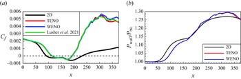


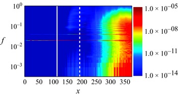

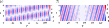
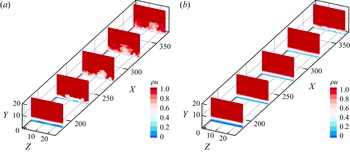
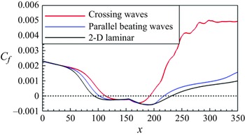


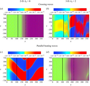


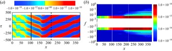


 Open access

