2.1. Governing equations

The three-dimensional compressible Navier–Stokes equations were employed as governing equations. These equations in the Cartesian coordinate system are as follows:

(2.1)\begin{equation}\frac{{\partial \boldsymbol{Q}}}{{\partial t}} + \frac{{\partial \boldsymbol{E}}}{{\partial x}} + \frac{{\partial \boldsymbol{F}}}{{\partial y}} + \frac{{\partial \boldsymbol{G}}}{{\partial z}} = \frac{{\partial {\boldsymbol{E}_{\boldsymbol{v}}}}}{{\partial x}} + \frac{{\partial {\boldsymbol{F}_{\boldsymbol{v}}}}}{{\partial y}} + \frac{{\partial {\boldsymbol{G}_{\boldsymbol{v}}}}}{{\partial z}},\end{equation}

where Q contains conservative variables; E, F and G are the x, y and z components of an inviscid flux, respectively; and E_v, F_v and G_v are the x, y and z components of a viscous flux, respectively.

(2.2)\begin{gather}\left. {\begin{array}{c@{}} \boldsymbol{Q} = {{(\begin{matrix} \rho &{\rho u}&{\rho v}&{\rho w}& e \end{matrix})}^\textrm{T}},\\ \boldsymbol{E} = {{(\begin{matrix} {\rho u}&{\rho {u^2} + p}&{\rho uv}&{\rho uw}&{(e + p)u} \end{matrix})}^\textrm{T}},\\ \boldsymbol{F} = {{(\begin{matrix} {\rho v}&{\rho vu}&{\rho {v^2} + p}&{\rho vw}&{({e + p} )v} \end{matrix})}^\textrm{T}},\\ \boldsymbol{G} = {{(\begin{matrix} {\rho w}&{\rho wu}&{\rho wv}&{\rho {w^2} + p}&{({e + p} )w} \end{matrix})}^\textrm{T}}, \end{array}} \right\}\end{gather}

(2.3)\begin{gather}\left. {\begin{array}{c@{}} {\boldsymbol{E}_{\boldsymbol{v}}} = {{(\begin{matrix} 0&{{\tau_{xx}}}&{{\tau_{xy}}}&{{\tau_{xz}}}&{{\beta_x}} \end{matrix})}^\textrm{T}},\\ {\boldsymbol{F}_{\boldsymbol{v}}} = {{(\begin{matrix} 0&{{\tau_{yx}}}&{{\tau_{yy}}}&{{\tau_{yz}}}&{{\beta_y}} \end{matrix})}^\textrm{T}},\\ {\boldsymbol{G}_{\boldsymbol{v}}} = {{(\begin{matrix} 0&{{\tau_{zx}}}&{{\tau_{zy}}}&{{\tau_{zz}}}&{{\beta_z}} \end{matrix})}^\textrm{T}}, \end{array}} \right\}\end{gather}

(2.4)\begin{gather}\left. {\begin{array}{c@{}} {\beta_x} = {\tau_{xx}}u + {\tau_{xy}}v + {\tau_{xz}}w - {q_x},\\ {\beta_y} = {\tau_{yx}}u + {\tau_{yy}}v + {\tau_{yz}}w - {q_y},\\ {{\beta_z} = {\tau_{zx}}u + \tau_{zy}}v + {\tau_{zz}}w - {q_z}, \end{array}} \right\}\end{gather}

where ρ is the density; u, v and w are the x, y and z components of velocity, respectively; τ is the component of a viscous stress tensor; and q is the heat flux. The total energy per unit volume e is written as follows in terms of an equation of state for ideal gases in the present study

(2.5)\begin{equation}e = \frac{p}{{\gamma - 1}} + \frac{1}{2}\rho ({u^2} + {v^2} + {w^2}).\end{equation}

Here, p and γ are the pressure and the specific heat ratio, respectively. In the present study, the specific heat ratio was set to be 1.4 by assuming air. Also, the Sutherland law (Sutherland Reference Sutherland1893) was employed for accounting the temperature dependence of the dynamic viscosity coefficient

(2.6)\begin{equation}\mu = {\mu _\infty }{\left( {\frac{T}{{{T_\infty }}}} \right)^{3/2}}\left( {\frac{{1 + C/{T_\infty }}}{{(T + C)/{T_\infty }}}} \right),\end{equation}

where C is constant for air in the Sutherland law (C = 110.4) and the Prandtl number was set to be 0.72. In addition, the three-dimensional Navier–Stokes equations in a general coordinate system are expressed as

(2.7)\begin{equation}\frac{{\partial \tilde{\boldsymbol{Q}}}}{{\partial t}} + \frac{{\partial \tilde{\boldsymbol{E}}}}{{\partial \xi }} + \frac{{\partial \tilde{\boldsymbol{F}}}}{{\partial \eta }} + \frac{{\partial \tilde{\boldsymbol{G}}}}{{\partial \zeta }} = \frac{{\partial {{\tilde{\boldsymbol{E}}}_{\boldsymbol{v}}}}}{{\partial \xi }} + \frac{{\partial {{\tilde{\boldsymbol{F}}}_{\boldsymbol{v}}}}}{{\partial \eta }} + \frac{{\partial {{\tilde{\boldsymbol{G}}}_{\boldsymbol{v}}}}}{{\partial \zeta }},\end{equation}

where

(2.8)\begin{gather}\left. {\begin{array}{* {20}{c}} \tilde{\boldsymbol{Q}} = \dfrac{Q}{J},\\ \tilde{\boldsymbol{E}} = \dfrac{1}{J}\left( {\dfrac{{\partial \xi }}{{\partial x}}E + \dfrac{{\partial \xi }}{{\partial y}}F + \dfrac{{\partial \xi }}{{\partial z}}G} \right),\\ \tilde{\boldsymbol{F}} = \dfrac{1}{J}\left( {\dfrac{{\partial \eta }}{{\partial x}}E + \dfrac{{\partial \eta }}{{\partial y}}F + \dfrac{{\partial \eta }}{{\partial z}}G} \right),\\ \tilde{\boldsymbol{G}} = \dfrac{1}{J}\left( {\dfrac{{\partial \zeta }}{{\partial x}}E + \dfrac{{\partial \zeta }}{{\partial y}}F + \dfrac{{\partial \zeta }}{{\partial z}}G} \right), \end{array}} \right\}\end{gather}

(2.9)\begin{gather}\left. {\begin{array}{* {20}{c}} {{\tilde{\boldsymbol{E}}}_{\boldsymbol{v}}} = \dfrac{1}{J}\left( {\dfrac{{\partial \xi }}{{\partial x}}{E_v} + \dfrac{{\partial \xi }}{{\partial y}}{F_v} + \dfrac{{\partial \xi }}{{\partial z}}{G_v}} \right),\\ {{\tilde{\boldsymbol{F}}}_{\boldsymbol{v}}} = \dfrac{1}{J}\left( {\dfrac{{\partial \eta }}{{\partial x}}{E_v} + \dfrac{{\partial \eta }}{{\partial y}}{F_v} + \dfrac{{\partial \eta }}{{\partial z}}{G_v}} \right),\\ {{\tilde{\boldsymbol{G}}}_{\boldsymbol{v}}} = \dfrac{1}{J}\left( {\dfrac{{\partial \zeta }}{{\partial x}}{E_v} + \dfrac{{\partial \zeta }}{{\partial y}}{F_v} + \dfrac{{\partial \zeta }}{{\partial z}}{G_v}} \right). \end{array}} \right\}\end{gather}

Here, J is the Jacobian, and ξ, η and ζ are the general coordinates.

2.2. Computational methods

The simulation was carried out by solving the Navier–Stokes equations on a boundary-fitted grid. The governing equations were non-dimensionalized by the density and speed of sound in the free stream and the sphere diameter. The convection and viscous terms were evaluated by the sixth-order adaptive central and upwind weighted essentially non-oscillatory scheme (WENOCU6-FP) proposed by Nonomura et al. (Reference Nonomura, Terakado, Abe and Fujii2015) and the sixth-order central difference method, respectively. The time integration was conducted by the third-order total variation-diminishing Runge–Kutta method proposed by Gottlieb & Shu (Reference Gottlieb and Shu1998). In the present study, the central difference of WENOCU6-FP was replaced by one of the splitting types proposed by Pirozzoli (Reference Pirozzoli2011) to stabilize the calculation. In particular, the WENO numerical flux F_weno for the convective term can be rewritten as the following expression:

(2.10)\begin{equation}{\boldsymbol{F}_{\boldsymbol{weno}}} = {\boldsymbol{F}_{{\boldsymbol{central}}\textit{-}{\boldsymbol{div}}}} + {\boldsymbol{F}_{{\boldsymbol{weno}}\textit{-}{\boldsymbol{dissipation}}}},\end{equation}

where F_central-div indicates the numerical flux corresponding to the sixth-order central difference, and F_{weno-dissipation} indicates the sixth-order dissipation term for the sixth-order WENOCU. Even though F_central is usually written in the form of a divergence, here it is replaced by the splitting form F_{central-split} of Pirozzoli (Reference Pirozzoli2011).

2.3. Computational grid

A computational grid around the sphere was generated as a body-fitted grid. The coordinate system and computational grid for Re = 300 are shown in figures 1 and 2, respectively. The diameter of the computational region was 100 times as large as that of the sphere. The region of 0.5d ≤ x ≤ 15d and (y ² + z ²)^0.5 ≤ 4d is the high-resolution region, where the high resolution of the computational grid was maintained and the wake structures were resolved. The grid size in the ζ direction was spread by 1.03 times from the minimum grid size, and the grid size became constant when the grid width reached Δζ_max = 0.05d at Re = 300 in the region at ζ ≤ 15d. The minimum grid size in the ζ direction was calculated using the following equation adopted by Johnson & Patel (Reference Johnson and Patel1999):

(2.11)\begin{equation}\Delta {\zeta _{min}} = \frac{{1.13}}{{\sqrt {Re} \times 10.0}}.\end{equation}

It is noted that the maximum grid size in ζ ≤ 15D for higher-Re cases was determined as follows:

(2.12)\begin{equation}\Delta {\zeta _{max}} = \Delta {\zeta _{max\_ref}}\frac{{\sqrt {R{e_{ref}}} }}{{\sqrt {Re} }}\textrm{,}\end{equation}

Figure 1. Coordinate system.

Figure 2. Computational grid (Re = 300).

where the reference value was Re_ref = 300, and Δξ_max and Δη_max were determined the same as in (2.12). The minimum grid size for the ξ and η direction was also determined the same as in (2.12). From 15d outward, the grid size increases by 1.2 times toward the outer boundary as a buffer region to prevent reflection of pressure waves. Note that the distance from the sphere to the outer boundary was much larger than that in previous incompressible simulations. The number of grid points for each Re and calculation conditions are shown in tables 1 and 2, respectively. The conditions investigated in the present study are the compressible low-Re flow because the goal of our project is the modelling of the compressible multiphase flow such as the exhaust jet of the rocket engines. For example, the exhaust jet of the solid rocket motor includes the alumina particles and aluminium droplets with a diameter of 1.1–200 μm (Shimada et al. Reference Shimada, Daimon and Sekino2006), and water droplets introduced by water injection are also included in the exhaust jet of the large-scale liquid rocket. The relative velocity between the particles and fluid becomes large when the particles pass the shock wave or shear layer, and the estimated flow condition around each particle is O(10¹)–O(10³) with the compressible flow. Hence, the knowledge of the compressible low-Re flow is essential for modelling of the compressible multiphase flow. Here, several cases were omitted to reduce the computational cost, for supersonic conditions because most conditions expected to be steady axisymmetric flows. Also, the flow field at M = 0.3 seems to be almost the same as incompressible flows.

Table 1. Number of grid points.

Table 2. Flow conditions.

The boundary conditions on the sphere surface are no-slip and adiabatic conditions. At the boundaries in the ξ and η directions, a periodic boundary condition on the six overlapped grid points was imposed. The inflow and outflow boundary conditions were imposed at the outer boundary where the flow goes inside and outside at one point inside the boundary, respectively. All flow variables were fixed to their free-stream values at the inflow boundaries. All the variables were extrapolated from one point inside of the boundary at the supersonic outflow boundaries. The density and the velocities were similarly extrapolated and the pressure was fixed to its free-stream values in the subsonic outflow condition. All the variables on the singular point on the x-axis were set to be an average of the nearest surrounding nodes.

3.1. Flow regime

According to studies of incompressible flow by Taneda (Reference Taneda1956), Magarvey & Bishop (Reference Magarvey and Bishop1961), Sakamoto & Haniu (Reference Sakamoto and Haniu1990) and Johnson & Patel (Reference Johnson and Patel1999), the flow structure at Re ≤ 1000 can be classified into six regimes. The flow is attached-laminar flow over the entire surface (fully attached flow) at Re < 24. Laminar separation occurs and a steady axisymmetric vortex ring forms behind the sphere at 24 < Re ≤ 210 (steady axisymmetric flow). The flow field is still steady, but axisymmetrical breakup occurs and the vortex ring assumes an asymmetric shape (steady planar–symmetric flow) at 211 ≤ Re ≤ 275. The flow over an isolated sphere becomes unsteady and hairpin vortex shedding begins at Re ≥ 275. The hairpin vortices are periodically released from the recirculation region of the sphere at 275 ≤ Re ≤ 420. The vortex shedding is highly organized (hairpin wake) in this Re range. The hairpin vortices are periodically released up to Re ≤ 800, but the heads of hairpin vortices roll in an azimuthal direction at 420 ≤ Re ≤ 800 (hairpin wake with azimuthal oscillation). The wake vortices become complicated and strongly random at Re ≥ 800. The wake consists of low-mode and high-mode structures and large-scale vortex structure forms and rolls in the azimuthal direction (helical wake).

Figure 3 shows the distribution of the flow regime in the Re–M plane under compressible conditions. The results of the previous studies by Nagata et al. (Reference Nagata, Nonomura, Takahashi, Mizuno and Fukuda2016), Riahi et al. (Reference Riahi, Meldi, Favier, Serre and Goncalves2018) and Sansica et al. (Reference Sansica, Robinet, Alizard and Goncalves2018) are shown for comparison with those of the present study. The result of Nagata et al. (Reference Nagata, Nonomura, Takahashi, Mizuno and Fukuda2016) is obtained by the three-dimensional DNS with a boundary-fitted coordinate (BFC) grid, the result of Riahi et al. (Reference Riahi, Meldi, Favier, Serre and Goncalves2018) is obtained the three-dimensional DNS with IBM, and the result of Sansica et al. (Reference Sansica, Robinet, Alizard and Goncalves2018) is obtained the three-dimensional GSA, respectively. In this plot, the seven different flow regimes described above are indicated as follows: fully attached flow (FA), steady axisymmetric flow (SA), steady planar-symmetric flow (SP), hairpin wake (HaW), hairpin wake 2 (HaW2), hairpin wake with azimuthal oscillation (HaWAO) and helical wake (HeW). However, in the article by Riahi et al. (Reference Riahi, Meldi, Favier, Serre and Goncalves2018), fully attached flow and hairpin wake with azimuthal oscillation did not appear. Those flow regimes seem to be included in steady axisymmetric flow and unsteady periodic flow (HaW in this article) in their articles, respectively. Fully attached flow also did not appear in the literature by Nagata et al. (Reference Nagata, Nonomura, Takahashi, Mizuno and Fukuda2016), but positions of the separation points were provided so that some of the conditions classified as steady axisymmetric flow in their article were re-classified here as fully attached flow. Figure 3 illustrates that the flow regime under the low subsonic flow at M = 0.3 is similar to that of incompressible flow. The regions of steady axisymmetric flow, steady planar–symmetric flow and the hairpin wake are slightly shifted toward the higher-Re side under high subsonic flow. This means that the steady regime expands to the higher-Re side. The relationship between flow regime and Re is drastically changed, and the flow field is significantly stabilized under transonic and supersonic conditions. Particularly, even non-axisymmetric flow does not appear for Re ≤ 1000 at M ≥ 1.5.

Figure 3. Distribution of flow regimes. Symbols: Nagata et al. (Reference Nagata, Nonomura, Takahashi, Mizuno and Fukuda2016) (BFC); Riahi et al. (Reference Riahi, Meldi, Favier, Serre and Goncalves2018) (IBM); Sansica et al. Reference Sansica, Robinet, Alizard and Goncalves2018 (GSA); present study (BFC). Colours: black, fully attached flow (FA); blue, steady axisymmetric flow (SA); light blue, steady planar–symmetric flow (SP); green, hairpin wake (HaW); green with purple, hairpin wake 2 (HaW2); dark green, hairpin wake with azimuthal oscillation (HaWAO); magenta, helical wake (HeW). Note that FA and HaWAO did not appear in Riahi et al. (Reference Riahi, Meldi, Favier, Serre and Goncalves2018), but it seems that those flow regimes are classified as steady axisymmetric flow and unsteady periodic flow (HaW in this article) in their articles, respectively.

3.2. Wake structure

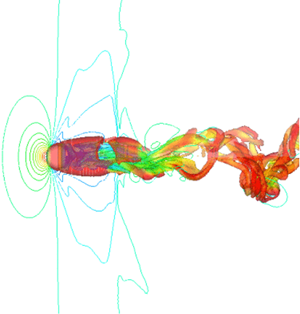
Figure 4 shows a wake structure visualized by the isosurface of the second invariant of the velocity gradient tensor, which is normalized by the free-stream velocity. Several kinds of wake structures appear at M ≤ 2.0 and Re ≤ 1000, and the wake structures become complex and simple as Re and M increase, respectively. The schematic diagram of the flow structure at supersonic conditions is also shown in the figure. As for the incompressible flow, a recirculation region is formed behind the sphere. The most different point between the subsonic and supersonic conditions is the existence of the shock wave. The bow shock is formed in the upstream of the sphere, and the shock standoff distance L_s is defined as the clearance between the bow shock and the upstream stagnation point. In addition, at moderate Re, the expansion wave and recompression wave are formed at around the position of the separation point and the end of the recirculation region, respectively.

Figure 4. Wake structure visualized by the second invariant of velocity gradient tensor $(Q/u_\infty ^2 = 5.0 \times {10^{ - 4}})$. Contours and iso-surface colours represent the pressure coefficient and velocity magnitude distributions, respectively.

Streamwise steady vortices are generated behind the sphere at Re = 250 and M = 0.3. The flow becomes unsteady and hairpin vortices are generated in the recirculation region of the sphere at Re = 300 and 500. When Re further increases to 750 and 1000, the wake vortices form a helical structure with a high mode and a low mode. The size of the recirculation region at M = 0.8 becomes large compared with that at M = 0.3, and the pressure coefficient distribution is different. The Re evolution of the flow patterns for M = 0.8 is similar at M = 0.3 in figure 4, but the wake structure at M = 0.8 seems to be more complicated. Thus, the critical Re for each flow pattern might be different between M = 0.3 and 0.8. However, the details of the value of critical Re for each flow pattern cannot be discussed due to a lack of DNS data in the Re direction. The compressibility effect on the wake vortices becomes obvious for M ≥ 0.95. The pressure coefficient distribution is drastically changed and a recompression wave can be observed around the end of the recirculation region. In this case, there is only a steady recirculation region, and no unsteady wake vortices are formed downstream of the sphere up to Re = 300. At Re = 500, streamwise vortices can be observed, similar to those at Re = 250 and M = 0.3, and the wake becomes helical at Re ≥ 750, as at M = 0.3 and 0.8, but its structure is more complex than that under subsonic conditions. A bow shock is formed upstream of the sphere at M ≥ 1.05, and those waves include expansion and recompression waves that become stronger as M increases. At M = 1.05, the flow behind the sphere remains steady state up to Re = 500, and hairpin structures appear at Re ≥ 750. Stabilization effects of the wake by compressibility become strong as M increases, and the wake is steady at M ≥ 1.5 and Re ≤ 1000.

In the present study, the hysteresis phenomena on the flow field were also explored based on the time variation of the lift coefficients. The hysteresis phenomena were not observed during our simulations in periodic cases (HaW, HaW2 and HaWAO). Also, no hysteresis phenomena such as temporal stabilization of the flow field at the investigated flow conditions were observed.

As shown in the above, the flow pattern is significantly influenced by the compressibility. For example, the wake at Re = 750 of M ≤ 0.95, the wake has a helical structure, but it becomes hairpin wake at M > 0.95. This kind of trend can also be observed at other Re cases investigated in the present study, and the flow field becomes steady at higher-M conditions, eventually. Therefore, the flow pattern at the higher-M condition is similar to that of the incompressible low-Re flows. Since there is an increase in the viscosity coefficient due to aerodynamic heating and decrease of the fluid velocity due to the bow shock, the local Re around the sphere seems to be decreased. However, the dynamics of the released wake vortices should be different due to the influence of the shock wave and the difference in Re based on the free-stream quantities. Detailed structures of the wake vortices are displayed in figure 5. The wake structures at Re = 300 of M = 0.3 and 0.8 is the simple hairpin structure. The wake structure of at Re = 500 of M = 0.3 is a hairpin structure, but the head of the hairpin vortices is oscillating around the streamwise direction. The wake structure at the same Re is helical wake at M = 0.8. The twisting of the vortex tube can be confirmed so that the wake structure seems to be that of the higher-Re one. Since the λ shock wave changes the position of the separation point and the stability of the wake, it is considered that the flow structure behind the sphere becomes different from the incompressible one. Meliga, Sipp & Chomaz (Reference Meliga, Sipp and Chomaz2010) showed a similar trend by global stability analysis with an axisymmetric approximation. They pointed out that the instability of the wake becomes strong because of the modification of the base flow. The direction of the head of the hairpin vortices is slightly swaying at Re = 500 of M = 0.3 and is rotating around the streamwise axis with a twist in vortex tubes at M = 0.8 as shown in figure 5. Also, there is a twist in the vortex tube so that the higher-frequency structure is included compared to the wake at Re = 500 of M = 0.3. The direction of the head of the hairpin vortices is fixed at M = 0.95 and the flow pattern is quite similar to that of the wake structure at Re = 300 of M = 0.3 and 0.8 but there are higher-frequency structures. In addition, the vortex structure under transonic and supersonic conditions at Re = 750 and 1000 are also similar to that of the wake structure at Re = 300 of M = 0.3, but there is the higher-frequency structure similar to the wake at Re = 500 of M = 0.95. Hence, there is the effect of the free-stream Re and a compressibility effect in the wake structure, and the wake structures at lower-Re in subsonic flow and that at higher-Re in transonic and supersonic flow seem to be similar but essentially different.

Figure 5. Effect of M and Re on the structure of wake vortices in each flow regime.

Figure 6 shows the influence of M on St of vortex shedding. The Strouhal number of vortex shedding was computed by the velocity fluctuation at the maximum turbulent kinetic energy (TKE) point in the downstream. There is a discrepancy between the present and previous results (Nagata et al. Reference Nagata, Nonomura, Takahashi, Mizuno and Fukuda2016) at M = 0.95 of Re = 300. The Strouhal number of vortex shedding at Re = 300 by Nagata et al. (Reference Nagata, Nonomura, Takahashi, Mizuno and Fukuda2016) was computed from the time variation of the lift coefficient. In addition, the amplitude of the lift coefficient at Re = 300 and M = 0.95 observed in the previous study was almost zero. It is considered that such small fluctuations did not appear as velocity fluctuations in the wake. The simulation was conducted for a long duration (378–585 flow through times). Also, we checked the effect of the data length on the fast Fourier transformation results. The difference in the first peak of St calculated by full data (excluding the initial phase of the computations) and 66 % of full data was around 1 %. Overall, St of vortex shedding increases as Re increases, and the critical M, where St of vortex shedding becomes zero, move to the higher-M side as Re increases. The Strouhal number of vortex shedding at Re = 300 decreases as M increases under subsonic conditions and rapidly approaches zero around M = 0.95 because there is no vortex shedding at Re = 300 and M ≥ 0.95. The trend of St of vortex shedding at Re = 500 is similar to that at Re = 300, but St of vortex shedding does not decrease up to M = 0.95 and sharply approaches zero around M = 1.0. The Strouhal number of vortex shedding decreases at 0.3 ≤ M ≤ 0.8 and there are no M effects on St of vortex shedding at 0.8 ≤ M ≤ 1.05. It appears that the decrease in St of vortex shedding at 0.3 ≤ M ≤ 0.8 is due to the difference in the wake structure. As shown in figure 4, the wake structure at M = 0.8 and 0.95 of Re = 750 is more complicated and has a larger amplitude (resembling a higher-Re condition) compared to that of M = 0.3 or under incompressible flows. The difference in the wake structure is considered to be caused by the difference in the position of the separation point. Flow separation in the high-subsonic and transonic cases is promoted by the effect of the expansion wave formed near the separation point. This results in the unsteadiness of the recirculation region and complicated vortex structure but St of vortex shedding decreases. Also, the flow field is strongly stabilized under the supersonic regime the same as lower-Re cases, and then St of vortex shedding becomes zero for M ≥ 1.2. The overall trend is similar to Re = 1000 but the different trend of increasing and decreasing St at around M = 1 is observed in this range. This peculiar tendency is considered to be caused by the interference of recompression wave and wake, and the expansion wave and boundary layer. Under sufficiently high-Re conditions, for example for Re ≥ 10⁵, the λ shock wave is formed, and flow separation occurs at around θ = 90°. The effect of the λ shock wave on the boundary layer seems to be limited at lower-Re conditions, as shown in figure 7(a), because the boundary layer on the sphere is quite thick and attenuates the λ shock wave. However, the complex interaction between the λ shock wave and the thick boundary layer might occur at the intermediate Re, which is at approximately 10³ (figure 7b). Although this phenomenon cannot be clarified only by the results of the present study, it can be clarified by performing a global stability analysis or resolvent analysis in future studies.

Figure 6. Effect of M on primary peak St of velocity fluctuation at the maximum TKE point: Re = 300 (St of C_L) (Nagata et al. Reference Nagata, Nonomura, Takahashi, Mizuno and Fukuda2016), Re = 300, Re = 500, Re = 750, Re = 1000 (present study).

Figure 7. Distribution of the divergence of the velocity near the sphere surface at M = 1.05. (a) Re = 250; (b) Re = 1000.

Figure 8 is the lift phase diagram, and the effect of M is illustrated for each Re. The variations in the lift coefficient occur only in the z-direction under subsonic conditions of Re = 300 because the direction of the hairpin vortices is fixed. The diagrams for M ≥ 0.95 converge to a single point because of the steady axisymmetric flow. At Re = 500, the flow regime of the subsonic flow becomes HaWAO or HeW so that there are variations of the lift coefficient in both z- and y-directions. Also, the amplitude of the lift coefficients for M = 0.3 is larger than that for M = 0.8. The difference in the amplitude of the lift coefficient is due to the difference in the flow regime. The randomness of the release location and direction of the wake vortices are strong in the case of HeW, and thus the effect of the oscillation of the wake on the lift coefficient seems to be smaller than that in the case of HaWAO. The amplitude of the lift coefficients at higher-Re conditions is reduced for the same reasons.

Figure 8. Effects of Re and M on the lift phase diagram. (a) Re = 300; (b) Re = 500; (c) Re = 750; (d) Re = 1000.

The effect of M on the relationship between wake oscillation and the amplitude of the lift coefficient can be seen at Re = 750 as shown in figures 4 and 8(c). The amplitude of the lift coefficients is almost the same at M = 0.3 and 0.8, but the amplitude of the wake at M = 0.8 is larger than that at M = 0.3. Destabilization effects of the sphere wake at subsonic flow have been suggested by Meliga et al. (Reference Meliga, Sipp and Chomaz2010). They showed that the critical Re for a transition from steady to unsteady flow decreases as M increases up to M ≈ 0.6 by a global stability analysis of axisymmetric wakes. Therefore, the flow regime at M = 0.8 of Re = 750 is HeW even though the flow regime at M = 0.3 of Re = 750 is a transitional regime between HaWAO and HeW. The difference in the flow regime results in the difference in the amplitude of the wake and the distribution of the turbulent kinetic energy. The effect of M on the turbulent kinetic energy in the wake will be discussed in § 3.3. At M = 0.95 of Re = 750, the amplitude of the lift coefficients is further reduced but the amplitude of the wake is larger than or similar to that of lower-M conditions, and the vortex structure is more complicated. Since the direction of the flow past the sphere is forced close the recirculation region because of the expansion wave, the recirculation region is stabilized and the amplitude of the lift coefficients is reduced. Conversely, the larger amplitude of the wake oscillation appears due to the interaction between the wake and recompression wave formed around the end of the recirculation region. Consequently, the amplitude of the wake oscillation of the transonic flow is larger than that of the shock-free flow in spite of the smaller variation of the lift coefficients.

3.3. Turbulent kinetic energy in the wake

Figure 9 shows the distribution of TKE in the wake region. The TKE was computed and normalized by free-stream kinetic energy as follows:

(3.1)\begin{equation}TKE = \frac{1}{2}\frac{{\mathop {{{u^{\prime}}^2}}\limits^{\_\_\_\_} + \mathop {{{v^{\prime}}^2}}\limits^{\_\_\_\_} + \mathop {{{w^{\prime}}^2}}\limits^{\_\_\_\_} }}{{u_\infty ^2}},\end{equation}

Figure 9. Normalized TKE distribution in the wake region: (a) Re = 500; (b) Re = 1000.

where $u^{\prime}$, $v^{\prime}$ and $w^{\prime}$ are the fluctuation components of fluid velocities which is defined as $u\mathrm{^{\prime}} = u - \bar{u}$. The overbar signifies the time-average value and the prime signifies the fluctuation value so that $\overline {u\mathrm{^{\prime}}} $ is equal to zero and $\overline {{{(u^{\prime})}^2}} $ is the mean square fluctuation. Also, the TKE was calculated in the high-resolution region (0.5d ≤ x ≤ 15d and $\sqrt {{y^2} + {z^2}} \le 4d$), and we determined the volume average by every Δx = 0.2d. Figure 9(a) illustrates that the TKE is continuously increasing approximately up to x = 2.5d. This is because of the end of the recirculation region of the unsteady case exists at around x = 2.0d. The TKE gradually decreases as the distance from the sphere increases. The TKE increases as M increases up to M ≤ 0.95, and it becomes less than 10⁻⁴ at M > 0.95 because the wake is steady. Figure 9(b) illustrates that the trend of the spatial distribution of the TKE at Re = 1000 is similar to that at Re = 500 and its value is higher than that at Re = 500. In addition, the TKE increases and decreases as M increase at M ≤ 0.95 and M ≥ 1.05, respectively. Therefore, it was confirmed that the TKE in the downstream of the sphere under higher-M conditions is larger than that under lower-M conditions with the same flow regime. In contrast, the TKE decreases as M increases at M ≥ 1.05 of Re = 1000 due to a change in the flow regime from helical wake to hairpin wake, and the TKE becomes less than 10⁻⁴ at M > 1.2 because of the steady wake. Hence, the compressibility effect not only leads to the stabilization of the flow field but also leads to the unsteadiness of the wake under an unsteady flow regime. The recirculation region is stabilized as M increases due to the expansion wave. On the other hand, the recompression wave formed in the downstream of the sphere facilitates a transition to turbulence. There is the recompression wave but the expansion wave is still weak at M = 0.95, and thus the TKE becomes maximum at around M = 1 of Re = 1000. The flow field becomes steady at M = 0.95 and M = 0.3 because of the low-Re conditions even though weak expansion waves.

4.1. Flow geometries

Figure 10 shows the M effects on the position of the separation point. The position of the separation point moves upstream as M increases up to M = 0.8 because the flow separation is promoted because of the λ shock formed at around θ = 90°. In contrast, the position of the separation point moves downstream as M increases at M > 0.8 because of the influence of the expansion wave. The flow direction behind the expansion wave changes to the direction toward the recirculation region, which reduces the flow separation, and its effect becomes strong under higher-M conditions. Also, the relative position of the separation point does not change with Re; that is, there is no clear influence of Re on the M effect in the separation point.

Figure 10. Dependence of separation point position on M and Re: (a) M dependence: Re = 300; Re = 500; Re = 750; Re = 1000.

Figure 11 shows the effects of M on the separation length. The separation length increases as M increases under subsonic conditions. The behaviour of the separation length is linked with the position of the separation point. The increment of the separation length rapidly increases at around the transonic regime, except at Re = 1000. On the other hand, the separation length decreases as M increases from the transonic to the supersonic regime, creating an inflection point in the separation length as M evolves. The inflection point moves to the higher-M side as Re increases because the separation length increases to its maximum value at around the critical M, which is the point at which the flow regime changes from steady to unsteady. Also, the maximum value of the separation length decreases as Re increases. A similar inflection point in the separation length exists at Re = 750 of M = 1.2, again because the inflection point appears when the flow changes from steady to unsteady. Therefore, the inflection point for M = 2.0 is considered to appear at Re ≥ 1000. It should be noted that the discrepancy in the length of the recirculation region at Re = 300 is due to the difference in the measurement method. In the study by Nagata et al. (Reference Nagata, Nonomura, Takahashi, Mizuno and Fukuda2016), the end of the recirculation region was explored on the x-axis. In the present study, on the other hand, the position of the end of the recirculation region is not limited to the x-axis. Since the shape of the recirculation region is skewed in the time-averaged field, and the end of the recirculation region is off-axis, the recirculation region provided by the present result is slightly longer than that of the result by Nagata et al. (Reference Nagata, Nonomura, Takahashi, Mizuno and Fukuda2016).

Figure 11. The Mach number dependence of recirculation region length. Re = 300; Re = 500; Re = 750; Re = 1000.

4.2. Distribution of surface stress coefficients

Figures 12 and 13 show the distribution of pressure and friction coefficients, respectively, at Re = 300 and 1000 for various M. In the present study, the pressure and friction coefficients were acquired from the time-averaged field and were averaged around the x-axis. Figure 12(a) illustrates that the pressure coefficient increases as M increases. Discontinuity due to the shock wave, which was confirmed in the previous study with a rotating sphere under compressible low-Re flow (Nagata et al. Reference Nagata, Nonomura, Takahashi, Mizuno and Fukuda2018b), is not observed. The minimum value of C_P exists at around θ = 90°, and its position moves downstream as M increases. Also, the minimum value of C_P decreases and increases as M increases, respectively, under subsonic and supersonic conditions. The minimum value of C_P at M = 2.0 is almost the same as C_P at the downstream stagnation point. The trend of the M effect on C_P distributions under subsonic conditions is similar to that of a cylinder at Re = 20 and 40 for M ≤ 0.5, as reported by Canuto & Taira (Reference Canuto and Taira2015). It should be noted that the change in the position of the separation point from M = 0 to 0.5 is less than 0.5°.

Figure 12. Pressure coefficient distribution on sphere surface: (a) Re = 300; (b) Re = 1000.

Figure 13. Friction coefficient distribution on sphere surface: (a) Re = 300; (b) Re = 1000.

The position where the C_P value at M ≤ 0.8 is minimized moves downstream as M increases, even though the position of the separation point moves upstream. Figure 12(b) illustrates that the influence of M on the C_P distribution at Re = 1000 is similar to that at Re = 300, but the influence of M on the C_P minimum becomes clearer. Figure 13 shows the distribution of C_f at Re = 300 and 1000 for various M. The value of C_f at Re = 300 becomes the maximum at around θ = 70° as shown in figure 13(a), and the peak position moves downstream as M increases. In addition, the peak value of C_f increases and decreases as M increases under subsonic and supersonic conditions, respectively. The maximum value of C_f is smaller than that under the lower-M cases under higher-M conditions in the upstream region, particularly under supersonic conditions, due to the bow shock. The dynamic viscosity coefficient also increases due to aerodynamic heating under supersonic conditions, but the effect of the deceleration of the flow is more effective. In contrast, C_f under the higher-M condition is larger at the downstream side where C_f becomes the maximum because the position of the separation point moves downstream as M increases at M ≥ 0.8. Figure 13(b) illustrates that a similar trend to Re = 300 can be observed at Re = 1000.

4.3. Drag coefficient

Figure 14 illustrates the effect of M on the drag coefficients at Re = 100, 300, 750 and 1000. The total drag coefficient C_D increases as M increases and its increment under transonic conditions is greater than that under subsonic and supersonic conditions due to increased wave drag. Under supersonic conditions, the increment of the drag coefficient becomes almost zero and is independent of M at around M > 1.5. A similar trend for inviscid hypersonic flows is well known as Oswatitsch's Mach number independence principle. The increment of the total drag coefficient by the effect of M is almost equivalent to the increase of the pressure component C_DP, as shown in figure 14(b). The effect of M on the pressure drag coefficient can be predicted by the Prandtl–Glauert transformation shown by the dotted curve up to high-subsonic conditions, and the increment of the pressure component at M > 0.9 is mainly according to the increment of the wave drag. However, the influence of M on the viscous component C_Dv is smaller than that on the pressure component. The viscous component slightly decreases as M increases under subsonic conditions because the position of the separation point moves upstream as M increases. The position of the separation point moves downstream under transonic conditions and the mean velocity gradient on the surface of the sphere increases. In contrast, the viscous component is almost constant under supersonic conditions despite the separation becoming delayed as M increases because the flow is decelerated at the bow shock, and the velocity gradient on the surface of the sphere decreases. The fluid viscosity increases due to increasing temperature, but the decrease in the velocity gradient is more effective, as shown in figure 13.

Figure 14. Effect of M on C_D: (a) total drag coefficient; (b) pressure drag coefficient; (c) viscous drag coefficient. Symbols: Re = 100 (Nagata et al. Reference Nagata, Nonomura, Takahashi, Mizuno and Fukuda2016), Re = 300, Re = 750, Re = 1000 (present study).

Figure 15 shows the relationship between Re and C_D at 0.3 ≤ M ≤ 2.0. The present results are compared to the drag curves predicted by the Loth model (Loth Reference Loth2008) and experimental drag data acquired by Sreekanth (Reference Sreekanth1961), Goin & Lawrence (Reference Goin and Lawrence1968), Zarin & Nicholls (Reference Zarin and Nicholls1971) and Bailey & Starr (Reference Bailey and Starr1976). There are experimental data in a wide range of Re and M, including the conditions investigated in the present study. Those drag data were acquired by wind tunnel experiments using a magnetic balance and suspension system, ballistic experiments and so on. Figure 15 illustrates that the drag coefficient increases as Re decreases for each value of M. The drag coefficients predicted by the drag model and DNS and measured by experiments show good agreement at M = 0.3. The present result agrees well with some experimental data at Re > 600 of M = 0.8, but the drag coefficient predicted by the Loth model is slightly lower than that by experiments and DNS. The difference between experimental and DNS data and the drag model becomes large as M increases under transonic conditions of 0.95 ≤ M ≤ 1.2, particularly in the low-Re conditions. The difference between experimental and DNS data also becomes large at lower-Re conditions because a no-slip boundary condition was used in the previous DNS study by Nagata et al. (Reference Nagata, Nonomura, Takahashi, Mizuno and Fukuda2016) despite the slightly rarefied regime. The drag model and experimental data show good agreement at M = 2.0, but the DNS overestimates the drag coefficient compared with the drag model and experimental data, particularly under the low-Re conditions. The overestimation by DNS is due to the influence of the no-slip boundary condition, and thus the difference between the DNS results and other data becomes small as Re increases. The Knudsen number at M = 2.0 of Re ≳ 250 is less than 0.001 so that the rarefaction effect is sufficiently small in that region, but there is a clear difference between the drag model and the experimental and DNS data.

Figure 15. Relationship between Re and drag coefficient: (a) M ≈ 0.3, (b) M ≈ 0.8, (c) M ≈ 0.95, (d) M ≈ 1.05, (e) M ≈ 1.2, (f) M ≈ 2.0. Symbols: Loth (Reference Loth2008), Goin & Lawrence (Reference Goin and Lawrence1968), Zarin & Nicholls (Reference Zarin and Nicholls1971), Bailey & Starr (Reference Bailey and Starr1976), Bailey & Hiatt (Reference Bailey and Hiatt1971), Bailey & Hiatt (Reference Bailey and Hiatt1972), Sreekanth (Reference Sreekanth1961), Nagata et al. (Reference Nagata, Nonomura, Takahashi, Mizuno and Fukuda2016), present study.

The drag model proposed by Loth (Reference Loth2008) is based on theoretical formulas, experimental formulas and empirical corrections, but the model includes interpolation and approximation due to a lack of experimental data in the transitional regime of continuum and rarefied flows. In other words, the drag model is not based on sufficient experimental data, and thus the accuracy of the drag model gets worse in the transitional condition. According to the original paper of the drag model, the drag model proposed in the previous study is valid in the flow conditions investigated in our study. Such flow conditions appear in compressible particle-laden flow, and the drag models are used in the multiphase flow analysis. The results of the present study, particularly in figure 15, indicate that the drag model proposed by the previous study requires correction to improve the prediction accuracy.

Figure 16 shows the increment of the total drag coefficient with increasing M. In the present study, ΔC_D was defined as follows:

(4.1)\begin{equation}\Delta {C_D} = {C_D}(Re,M) - {C_D}(Re,M = 0),\end{equation}

where C_D(Re, M) indicates the drag coefficient predicted by the present DNS or previous experiments, and C_D (Re, M = 0) indicates the drag coefficient under the incompressible flow, which was predicted by the drag model proposed by Clift & Gauvin (Reference Clift and Gauvin1971). Figure 16(a) illustrates that ΔC_D increases as M increase at M ≥ 0.3, and its value appears to be only a function of M. The increment of ΔC_D under transonic conditions is in particular larger than that under subsonic and supersonic conditions. The increment of ΔC_D under subsonic conditions is caused by a compressibility effect, which can be explained by the Prandtl–Glauert transformation, and the pressure drag increases due to a decrease of the attached region, as illustrated in figure 14(b) and figure 10. The increment of the wave drag is almost constant at M > 1.5 and moderate Re; hence, the increment of ΔC_D becomes small under higher-M conditions but also under low-Re conditions. At M = 0.3, ΔC_D is negative because the drag coefficient at M = 0.3 is slightly smaller than that under incompressible flow conditions, due to the position of the separation point existing upstream compared to that under incompressible flows. The position of the separation point under lower-Re conditions exists downstream compared with that under higher-Re conditions, and thus the decrement of ΔC_D is larger under lower-Re conditions. Figure 16(b) shows ΔC_D as calculated using published experimental data. In this case, ΔC_D is approximately characterized by M at M < 1.5, but Re dependence appears at M = 2.0. The value of ΔC_D decreases as Re decreases for lower-Re conditions of M = 2.0, particularly at Re ≤ 200, because the Knudsen number based on the free-stream velocity and the sphere diameter is greater than 0.01 at Re ≤ 200 and M = 2.0. Hence, the slip effect on the wall caused by the rarefaction effect gradually strengthens as Re decreases.

Figure 16. Increment of drag coefficient by M effect: (a) present study: Re = 300, Re = 500, Re = 750, Re = 1000; (b) published experimental results: Re = 50, Re = 100, Re = 200, Re = 500, Re = 1000, Re = 5000, Re = 10 000, Re = 100 000 (black symbols, Bailey & Hiatt Reference Bailey and Hiatt1972; grey symbols, Bailey & Starr Reference Bailey and Starr1976).