


1. Introduction
Dense turbulent suspensions play a pivotal role in a wide range of industrial applications and natural phenomena such as pneumatic conveying, debris flow, sediment transport and snow avalanches. Here, we term a suspension ‘dense’ when inter-particle interactions are frequent compared with the typical response time of the particles, and ‘dilute’ otherwise (Clift, Grace & Weber Reference Clift, Grace and Weber2005). Despite their prevalence, understanding these complex systems remains elusive due to the intricate interplay of multiple physical mechanisms across different scales. Traditionally, research studies have focused on either dense, viscous suspensions (Guazzelli, Morris & Pic Reference Guazzelli, Morris and Pic2011) or dilute, turbulent ones (Balachandar & Eaton Reference Balachandar and Eaton2010). The study of dense turbulent suspensions has been thwarted by the physical complexities that arise when both inertial effects and inter-particle interactions are combined, and by the difficulty of both measuring and simulating the system behaviour. Recent advances in experimental methods (e.g. refractive index matching and medical imaging) and numerical models (such as particle-resolved simulations) have enabled the investigation of transitional and turbulent dense suspensions, for example in pipe flows (Matas, Morris & Guazzelli Reference Matas, Morris and Guazzelli2003; Hogendoorn & Poelma Reference Hogendoorn and Poelma2018; Agrawal, Choueiri & Hof Reference Agrawal, Choueiri and Hof2019; Hogendoorn et al. Reference Hogendoorn, Breugem, Frank, Bruschewski, Grundmann and Poelma2023), channel flows (Picano, Breugem & Brandt Reference Picano, Breugem and Brandt2015; Wang et al. Reference Wang, Peng, Guo and Yu2016; Zade et al. Reference Zade, Costa, Fornari, Lundell and Brandt2018; Olivieri et al. Reference Olivieri, Brandt, Rosti and Mazzino2020; Fong & Coletti Reference Fong and Coletti2022), boundary layers (Baker & Coletti Reference Baker and Coletti2019), decaying turbulence (Zhang & Rival Reference Zhang and Rival2018) and sediment transport (Vowinckel et al. Reference Vowinckel, Zhao, Zhu and Meiburg2023). The nature of the methodologies, however, entails limitations on the accessible regimes, specifically on the particle properties and concentration, and on the system scale. Thus, while progress is fast, the area can still be considered in its infancy.
An additional layer of complexity arises when particles are confined at fluid interfaces, where their dynamics differs substantially from that in the bulk (Singh & Joseph Reference Singh and Joseph2005; Madivala, Fransaer & Vermant Reference Madivala, Fransaer and Vermant2009; Magnaudet & Mercier Reference Magnaudet and Mercier2020). Previous studies exploring the behaviour of particles at interfaces have mostly focused on low-inertia or microscopic colloidal systems (Hoekstra et al. Reference Hoekstra, Vermant, Mewis and Fuller2003; Fuller & Vermant Reference Fuller and Vermant2012; Garbin Reference Garbin2019). On the other hand, dense turbulent interfacial suspensions are present in both industrial and natural settings, for example froth flotation in process engineering and in patches of marine plastics. Multiple mechanisms may then superpose; for example, particle clustering may manifest itself due to hydrodynamic interactions (Brown & Jaeger Reference Brown and Jaeger2014), inertial effects (Brandt & Coletti Reference Brandt and Coletti2022) and capillarity (Protière Reference Protière2023).
In our prior work (Shin & Coletti Reference Shin and Coletti2024), we examined the interactions of non-Brownian, monodisperse spherical particles at the interface of quasi-two-dimensional (Q2-D) turbulent liquid layers. By systematically varying parameters such as turbulence intensity, interfacial tension, particle size and concentration, we investigated the clustering propensity, cluster size and the particles’ mean kinetic energy, all influenced by the interplay of capillarity, drag and lubrication forces. The balance of these forces was quantified by two key non-dimensional parameters: the capillary number ( $Ca$
) and the areal fraction (
$Ca$
) and the areal fraction ( $\phi$
). The former is the ratio between the drag force pulling nearby particles apart and the capillary attraction keeping them together. The latter is related to the ratio between the footprint of all particles in the domain and the area of the same domain. We proposed a phase diagram identifying three distinct regimes in the
$\phi$
). The former is the ratio between the drag force pulling nearby particles apart and the capillary attraction keeping them together. The latter is related to the ratio between the footprint of all particles in the domain and the area of the same domain. We proposed a phase diagram identifying three distinct regimes in the $Ca-\phi$
space, each associated with a different clustering behaviour and kinetic energy of the particles.
$Ca-\phi$
space, each associated with a different clustering behaviour and kinetic energy of the particles.
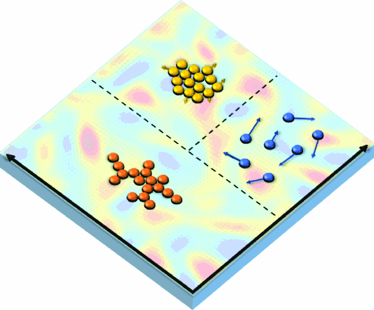
Building on this foundation, the present study explores in detail the individual and collective particle dynamics within these regimes. By analysing the spatio-temporal scales and structure of clusters as well as the Lagrangian particle motion, we elucidate the underlying mechanisms governing the aggregation and dispersion in the various regimes. The paper is organised as follows. Section 2 presents the experimental set-up, defines the physical parameters and describes the measurement approach and data processing. Section 3 discusses the results in terms of cluster properties (3.1) and particle motion (3.2). Section 4 draws conclusions and offers an outlook for future work.
2. Methods
We use a conductive fluid consisting of a 10 % CuSO $_{4}$
aqueous solution by mass, with density
$_{4}$
aqueous solution by mass, with density $\rho _{f}=1.08\,\rm g\, ml^-{^1}$
and kinematic viscosity
$\rho _{f}=1.08\,\rm g\, ml^-{^1}$
and kinematic viscosity $\nu = 1.0 \times 10^{-6}\,\rm m^{2}\,s^{-1}$
. The conductive fluid is contained in a 320
$\nu = 1.0 \times 10^{-6}\,\rm m^{2}\,s^{-1}$
. The conductive fluid is contained in a 320 $\times$
320 mm
$\times$
320 mm $^{2}$
tray, placed above an 8
$^{2}$
tray, placed above an 8 $\times$
8 magnet array arranged in a checkerboard pattern with alternating polarities. The flow is induced by applying DC current through copper electrodes at opposite sides of the tray, generating Lorentz forces in the horizontal direction. The magnets are spaced at a centre-to-centre distance of 35 mm, defining the forcing scale
$\times$
8 magnet array arranged in a checkerboard pattern with alternating polarities. The flow is induced by applying DC current through copper electrodes at opposite sides of the tray, generating Lorentz forces in the horizontal direction. The magnets are spaced at a centre-to-centre distance of 35 mm, defining the forcing scale $L_{F}$
. This set-up aligns with configurations frequently employed in prior Q2-D turbulence studies, and was detailed extensively in our previous study (Shin, Coletti & Conlin Reference Shin, Coletti and Conlin2023).
$L_{F}$
. This set-up aligns with configurations frequently employed in prior Q2-D turbulence studies, and was detailed extensively in our previous study (Shin, Coletti & Conlin Reference Shin, Coletti and Conlin2023).
We employ two distinct fluid layer set-ups and two sizes of polyethylene spheres (Cospheric WPMS-1.00, CPB-0.96). The set-ups include: a single-layer (SL) configuration, where spheres are placed at the free surface of a 7 mm-deep conductive layer: and double-layer (DL) configurations (DL1 and DL2), with a 2 mm-thick mineral oil layer on top of an 8 mm-thick conductive layer, where the spheres are at the liquid–liquid interface. In DL1 and DL2 the fluid layers are identical, but different particle sizes are used. Particles are introduced in varying quantities to adjust the areal fraction $\phi \equiv N_{p} (\pi d_{p}^{2} / 4) / A_{FOV}$
, where
$\phi \equiv N_{p} (\pi d_{p}^{2} / 4) / A_{FOV}$
, where $N_{p}$
is the time-averaged number of particles in the field of view of area
$N_{p}$
is the time-averaged number of particles in the field of view of area $A_{FOV}$
, and
$A_{FOV}$
, and ${d}_p$
is the particle diameter. To explore the full range of concentrations from fully dilute to fully dense, we vary
${d}_p$
is the particle diameter. To explore the full range of concentrations from fully dilute to fully dense, we vary $\phi$
from 1 % to 71 %.
$\phi$
from 1 % to 71 %.
To ensure consistency across experiments, we verify that the Bond number ( $Bo$
) and the Stokes number (
$Bo$
) and the Stokes number ( $St$
) are both much smaller than 1 in all cases. The small Bond number,
$St$
) are both much smaller than 1 in all cases. The small Bond number, $Bo \equiv (\rho _{f} - \rho _{p}) g d_{p}^{2} / (4 \gamma )$
, with
$Bo \equiv (\rho _{f} - \rho _{p}) g d_{p}^{2} / (4 \gamma )$
, with $\rho _{p}$
the particle density, g is the gravitational acceleration and
$\rho _{p}$
the particle density, g is the gravitational acceleration and $\gamma$
the interfacial tension, indicates that interfacial distortion due to buoyancy is negligible. The small Stokes number,
$\gamma$
the interfacial tension, indicates that interfacial distortion due to buoyancy is negligible. The small Stokes number, $St \equiv \tau _{p} u_{rms,f} / L_{F}$
, where
$St \equiv \tau _{p} u_{rms,f} / L_{F}$
, where $\tau _{p} = \rho _{p} d_{p}^{2} / (18 \mu )$
is the particle response time,
$\tau _{p} = \rho _{p} d_{p}^{2} / (18 \mu )$
is the particle response time, $\mu$
is the dynamic viscosity of the carrying fluid (or simply fluid viscosity) and
$\mu$
is the dynamic viscosity of the carrying fluid (or simply fluid viscosity) and $u_{rms,f}$
is the root-mean-square velocity of the flow
$u_{rms,f}$
is the root-mean-square velocity of the flow $u_{rms,f} = \langle \boldsymbol{u}(\boldsymbol{x},t) \cdot \boldsymbol{u}(\boldsymbol{x},t) \rangle _{\boldsymbol{x},t}^{1/2}$
, indicates that particle inertia is insignificant in comparison with the energetic flow scales, justifying the assumption of a Stokesian dynamics. The capillary number is defined as
$u_{rms,f} = \langle \boldsymbol{u}(\boldsymbol{x},t) \cdot \boldsymbol{u}(\boldsymbol{x},t) \rangle _{\boldsymbol{x},t}^{1/2}$
, indicates that particle inertia is insignificant in comparison with the energetic flow scales, justifying the assumption of a Stokesian dynamics. The capillary number is defined as $Ca \equiv 6 \sqrt {2} \pi {d}_p^{6} u_{rms} / (\Theta L_F)$
, where
$Ca \equiv 6 \sqrt {2} \pi {d}_p^{6} u_{rms} / (\Theta L_F)$
, where $\Theta = 12 \gamma h_{qp}^{2} {d}_p^{3} / \mu$
, with
$\Theta = 12 \gamma h_{qp}^{2} {d}_p^{3} / \mu$
, with $\gamma$
the interfacial tension and
$\gamma$
the interfacial tension and $h_{qp}$
the amplitude of the quadrupole mode of the interfacial distortion, whose measurement was discussed in our previous study (Shin & Coletti Reference Shin and Coletti2024). Note that our formulation of
$h_{qp}$
the amplitude of the quadrupole mode of the interfacial distortion, whose measurement was discussed in our previous study (Shin & Coletti Reference Shin and Coletti2024). Note that our formulation of $Ca$
is based on an average extensional strain rate evaluated at a characteristic particle separation; therefore, an increase in
$Ca$
is based on an average extensional strain rate evaluated at a characteristic particle separation; therefore, an increase in $Ca$
indicates that, on average, viscous (or turbulent) drag increasingly overcomes capillary forces, resulting in diminished particle cohesion. Further details of the experimental parameters are provided in table 1.
$Ca$
indicates that, on average, viscous (or turbulent) drag increasingly overcomes capillary forces, resulting in diminished particle cohesion. Further details of the experimental parameters are provided in table 1.
Table 1. Summary of the experimental parameters.
We use a Phantom VEO 640 CMOS camera to record 100-second sequences at rates of 100–240 frames per second, ensuring that inter-frame particle displacements are confined to approximately 5 pixels or $\sim 1\,\rm mm$
. The imaging focuses on the central zone of the tray, approximately
$\sim 1\,\rm mm$
. The imaging focuses on the central zone of the tray, approximately $L_F$
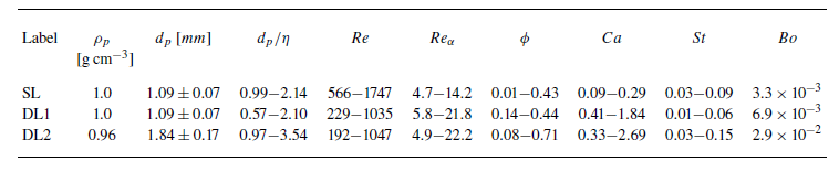
away from its boundaries, to minimise edge effects. The field of view captures a spatially and temporally homogeneous system of particles, with temporal fluctuations in the number of imaged particles typically smaller than 1 % of the mean. Particle centroids are tracked with sub-pixel accuracy using an in-house code, allowing us to reconstruct their Lagrangian trajectories. We define clusters as groups of adjacent particles. For their identification we employ the Density-Based Spatial Clustering of Applications with Noise (DBSCAN) algorithm (Ester et al. Reference Ester, Kriegel, Sander and Xu1996), setting a search radius around each particle centroid to determine adjacency, with a minimum requirement of four neighbours. This is preferred to cluster identification strategies as the Voronoi tessellation (Baker et al. Reference Baker, Frankel, Mani and Coletti2017; Liu et al. Reference Liu, Shen, Zamansky and Coletti2020) requires defining a threshold dependent on the system concentration and excluded volume effects. The search radius
$L_F$
away from its boundaries, to minimise edge effects. The field of view captures a spatially and temporally homogeneous system of particles, with temporal fluctuations in the number of imaged particles typically smaller than 1 % of the mean. Particle centroids are tracked with sub-pixel accuracy using an in-house code, allowing us to reconstruct their Lagrangian trajectories. We define clusters as groups of adjacent particles. For their identification we employ the Density-Based Spatial Clustering of Applications with Noise (DBSCAN) algorithm (Ester et al. Reference Ester, Kriegel, Sander and Xu1996), setting a search radius around each particle centroid to determine adjacency, with a minimum requirement of four neighbours. This is preferred to cluster identification strategies as the Voronoi tessellation (Baker et al. Reference Baker, Frankel, Mani and Coletti2017; Liu et al. Reference Liu, Shen, Zamansky and Coletti2020) requires defining a threshold dependent on the system concentration and excluded volume effects. The search radius $\epsilon {d}_p$
, where
$\epsilon {d}_p$
, where $\epsilon$
is the contact distance between centroids of adjacent pairs of particles normalised by the mean particle diameter, is determined by analysing a low-
$\epsilon$
is the contact distance between centroids of adjacent pairs of particles normalised by the mean particle diameter, is determined by analysing a low- $Ca$
case where tightly bound clusters and a few single particles coexist. We then plot the nearest-neighbour distance for each particle in ascending order and identify the transition point where the distribution flattens (figure 1
a). The results are only weakly dependent on the precise value of
$Ca$
case where tightly bound clusters and a few single particles coexist. We then plot the nearest-neighbour distance for each particle in ascending order and identify the transition point where the distribution flattens (figure 1
a). The results are only weakly dependent on the precise value of $\epsilon$
. This corresponds to an inter-particle gap much smaller than
$\epsilon$
. This corresponds to an inter-particle gap much smaller than ${d}_p$
and comparable to the expected thickness of a lubrication layer between capillarity-bonded particles.
${d}_p$
and comparable to the expected thickness of a lubrication layer between capillarity-bonded particles.
Figure 1(b) displays a resulting example of cluster detection at $Ca=0.33$
and
$Ca=0.33$
and $\phi =0.44$
based on
$\phi =0.44$
based on $\epsilon =1.20$
, our choice for this particle type based on the nearest-neighbour distance distribution. We apply the same value of
$\epsilon =1.20$
, our choice for this particle type based on the nearest-neighbour distance distribution. We apply the same value of $\epsilon$
to all cases with the same type of particles: a search radius of 1.25
$\epsilon$
to all cases with the same type of particles: a search radius of 1.25 ${d}_p$
is used for SL and DL1 and 1.20
${d}_p$
is used for SL and DL1 and 1.20 ${d}_p$
for DL2.
${d}_p$
for DL2.
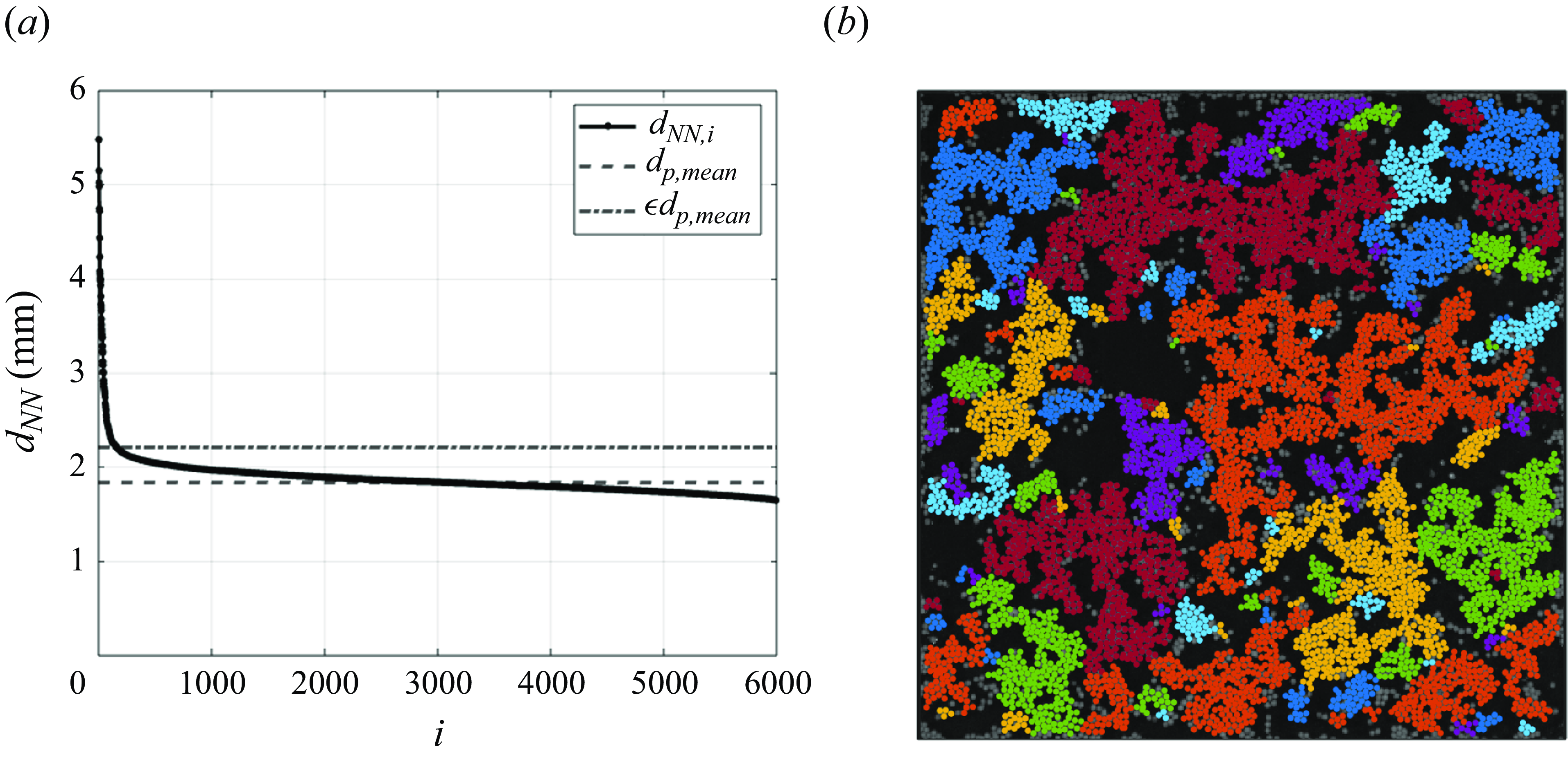
Figure 1. Choice of a searching radius. (a) Distance to the nearest neighbour $d_{NN}$
sorted in descending order. The dashed line represents the mean particle diameter (
$d_{NN}$
sorted in descending order. The dashed line represents the mean particle diameter ( ${d}_p$
), and the dash-dot line indicates the cutoff distance used to identify clustered neighbours. (b) An example of cluster detection from the corresponding experiment at
${d}_p$
), and the dash-dot line indicates the cutoff distance used to identify clustered neighbours. (b) An example of cluster detection from the corresponding experiment at $Ca = 0.33$
and
$Ca = 0.33$
and $\phi = 0.44$
. Particles within the same cluster are indicated with the same colour.
$\phi = 0.44$
. Particles within the same cluster are indicated with the same colour.
To assess turbulence intensity under different electromagnetic forcing, we perform separate particle image velocimetry (PIV) experiments where the fluid is exclusively laden with polyethylene microspheres as tracers ( $d_{p} = 75 - 90\ \unicode{x03BC}$
m, Cospheric UVPMS-BG-1.00). These stay at the free surface (SL) or at the liquid–liquid interface (DL), similarly to the millimetric particles. We calculate the Reynolds number
$d_{p} = 75 - 90\ \unicode{x03BC}$
m, Cospheric UVPMS-BG-1.00). These stay at the free surface (SL) or at the liquid–liquid interface (DL), similarly to the millimetric particles. We calculate the Reynolds number $Re \equiv u_{rms,f} L_F / \nu$
based on
$Re \equiv u_{rms,f} L_F / \nu$
based on $u_{rms,f}$
, which is varied by adjusting the electrical current from 0.09 to 1.00 A. The level of forcing falls within the turbulent regime (Shin et al. Reference Shin, Coletti and Conlin2023), with Kolmogorov scales
$u_{rms,f}$
, which is varied by adjusting the electrical current from 0.09 to 1.00 A. The level of forcing falls within the turbulent regime (Shin et al. Reference Shin, Coletti and Conlin2023), with Kolmogorov scales $\eta$
comparable to
$\eta$
comparable to ${d}_p$
(table 1). The outer-scale Reynolds number
${d}_p$
(table 1). The outer-scale Reynolds number $Re_{\alpha }=u_{rms,f}/(\alpha L_F)$
, where
$Re_{\alpha }=u_{rms,f}/(\alpha L_F)$
, where $\alpha$
is the friction coefficient, equals or exceeds the approximate threshold
$\alpha$
is the friction coefficient, equals or exceeds the approximate threshold $Re_{\alpha }\approx 5$
(figure 2
a) which ensures fully developed 2-D turbulence (Shin et al. Reference Shin, Coletti and Conlin2023). The scaling of the third-order longitudinal structure function
$Re_{\alpha }\approx 5$
(figure 2
a) which ensures fully developed 2-D turbulence (Shin et al. Reference Shin, Coletti and Conlin2023). The scaling of the third-order longitudinal structure function $\langle \delta u_L^3\rangle$
exhibits the expected transition from
$\langle \delta u_L^3\rangle$
exhibits the expected transition from $\sim r^3$
to
$\sim r^3$
to $\sim r$
for separations
$\sim r$
for separations $r\approx L_F$
(figure 2
b), while the energy spectrum is consistent with the scaling
$r\approx L_F$
(figure 2
b), while the energy spectrum is consistent with the scaling $E \sim k^{-3}$
in the wavenumber range
$E \sim k^{-3}$
in the wavenumber range $k\gt k_F$
, where
$k\gt k_F$
, where $k_F=2\pi /L_F$
(figure 2
c); see Boffetta & Ecke (Reference Boffetta and Ecke2012). The limited size of the system does not allow to ascertain the expected scaling
$k_F=2\pi /L_F$
(figure 2
c); see Boffetta & Ecke (Reference Boffetta and Ecke2012). The limited size of the system does not allow to ascertain the expected scaling $E \sim k^{-5/3}$
for
$E \sim k^{-5/3}$
for $k\lt k_F$
.
$k\lt k_F$
.
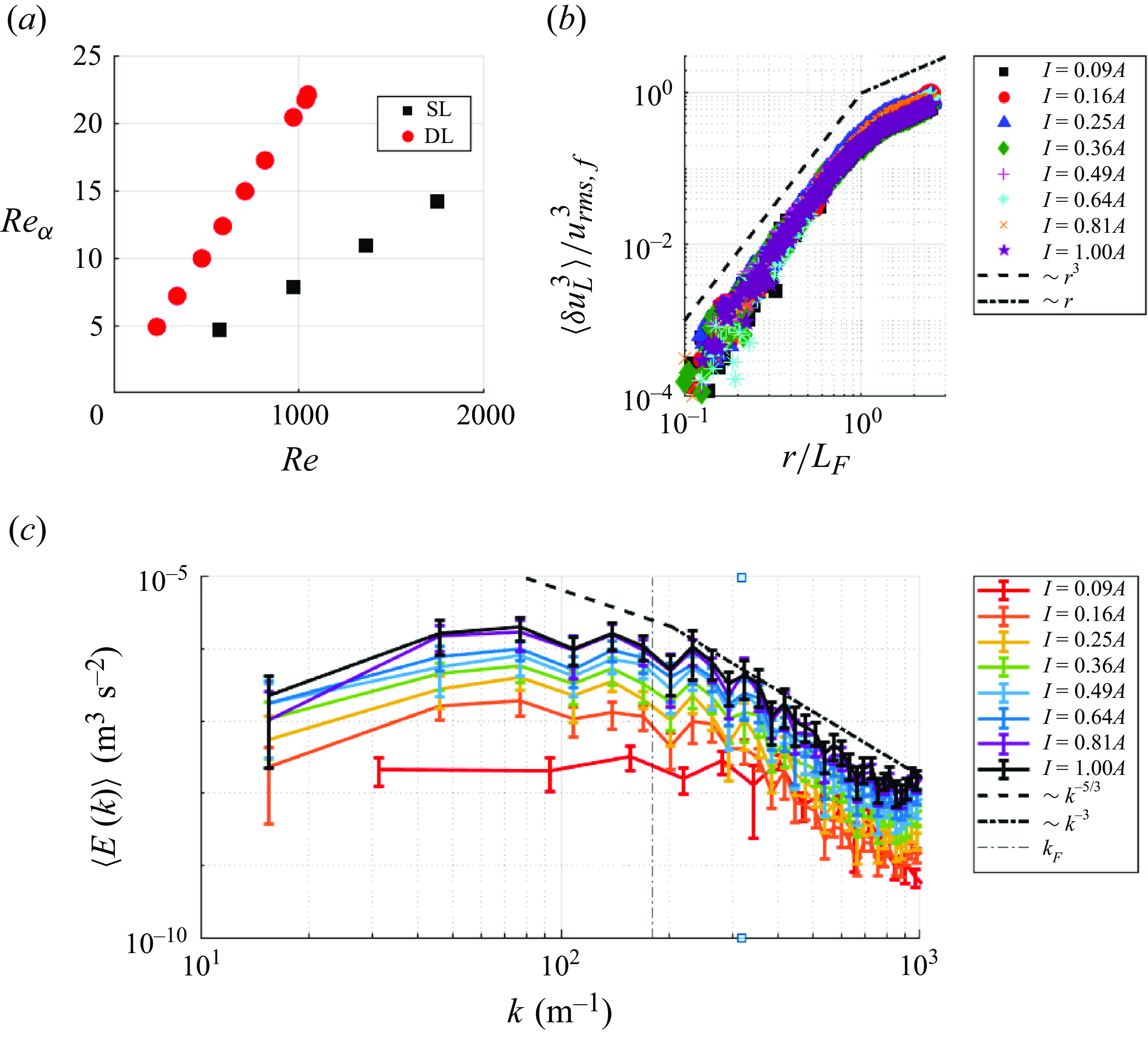
Figure 2. (a) Range of Reynolds numbers $Re$
and
$Re$
and $Re_{\alpha }$
for the SL (black) and DL (red) configurations in this study. (b) Normalised third-order longitudinal structure function,
$Re_{\alpha }$
for the SL (black) and DL (red) configurations in this study. (b) Normalised third-order longitudinal structure function, $\langle \delta u_L^3\rangle / u_{rms,f}^3$
), and (c) energy spectrum,
$\langle \delta u_L^3\rangle / u_{rms,f}^3$
), and (c) energy spectrum, $\langle E(k) \rangle$
, at varying levels of forcing for the DL configuration.
$\langle E(k) \rangle$
, at varying levels of forcing for the DL configuration.
To provide a baseline for comparing the effects of particle–particle and particle–fluid interactions, we use random sequential adsorption (RSA) to virtually distribute non-overlapping circles in the two-dimensional (2-D) domain (Evans Reference Evans1993). The circle sizes are drawn from a normal distribution matching the particle size distribution in our experiments (approximately Gaussian with standard deviation listed in table 1). We generate random configurations up to $\phi =0.54$
, close to the saturation coverage of 0.547 (Hinrichsen, Feder & Jøssang Reference Hinrichsen, Feder and Jøssang1990). This RSA approach mimics a scenario devoid of any forcing length scale and inter-particle interactions (except for the excluded volume). Note that our DBSCAN clustering criterion – using the same threshold
$\phi =0.54$
, close to the saturation coverage of 0.547 (Hinrichsen, Feder & Jøssang Reference Hinrichsen, Feder and Jøssang1990). This RSA approach mimics a scenario devoid of any forcing length scale and inter-particle interactions (except for the excluded volume). Note that our DBSCAN clustering criterion – using the same threshold $\epsilon$
and a minimum requirement of four neighbours – is applied consistently to the RSA-generated configurations.
$\epsilon$
and a minimum requirement of four neighbours – is applied consistently to the RSA-generated configurations.
3. Results
As we demonstrated in Shin & Coletti (Reference Shin and Coletti2024), the behaviour of the particles at the fluid interface is governed by the interplay of capillary, drag and lubrication forces. The ratio between those defines a $Ca-\phi$
phase space that captures different regimes of clustering and particle kinetic energy. Capillarity act as a cohesive mechanism between particles, and it is counteracted by viscous drag which disrupts cluster formation, especially in turbulent flows with locally high strain rates. For large
$Ca-\phi$
phase space that captures different regimes of clustering and particle kinetic energy. Capillarity act as a cohesive mechanism between particles, and it is counteracted by viscous drag which disrupts cluster formation, especially in turbulent flows with locally high strain rates. For large $Ca$
, the drag dominates promoting cluster break-up, particularly at relatively low (henceforth, moderately dense) concentrations. Conversely, when both
$Ca$
, the drag dominates promoting cluster break-up, particularly at relatively low (henceforth, moderately dense) concentrations. Conversely, when both $\phi$
and
$\phi$
and $Ca$
are large, lubrication prevents particles from separating, allowing for large and stable clusters that move relatively slowly. Quantitatively, we identify three distinct regimes in the
$Ca$
are large, lubrication prevents particles from separating, allowing for large and stable clusters that move relatively slowly. Quantitatively, we identify three distinct regimes in the $Ca-\phi$
space: (i) capillary-driven clustering for
$Ca-\phi$
space: (i) capillary-driven clustering for $Ca \lt 1$
, (ii) drag-driven break-up for
$Ca \lt 1$
, (ii) drag-driven break-up for $Ca \gt 1$
and
$Ca \gt 1$
and $\phi \lt 0.40$
and (iii) lubrication-driven clustering for
$\phi \lt 0.40$
and (iii) lubrication-driven clustering for $Ca \gt 1$
and
$Ca \gt 1$
and $\phi \gt 0.40$
(figure 3).
$\phi \gt 0.40$
(figure 3).
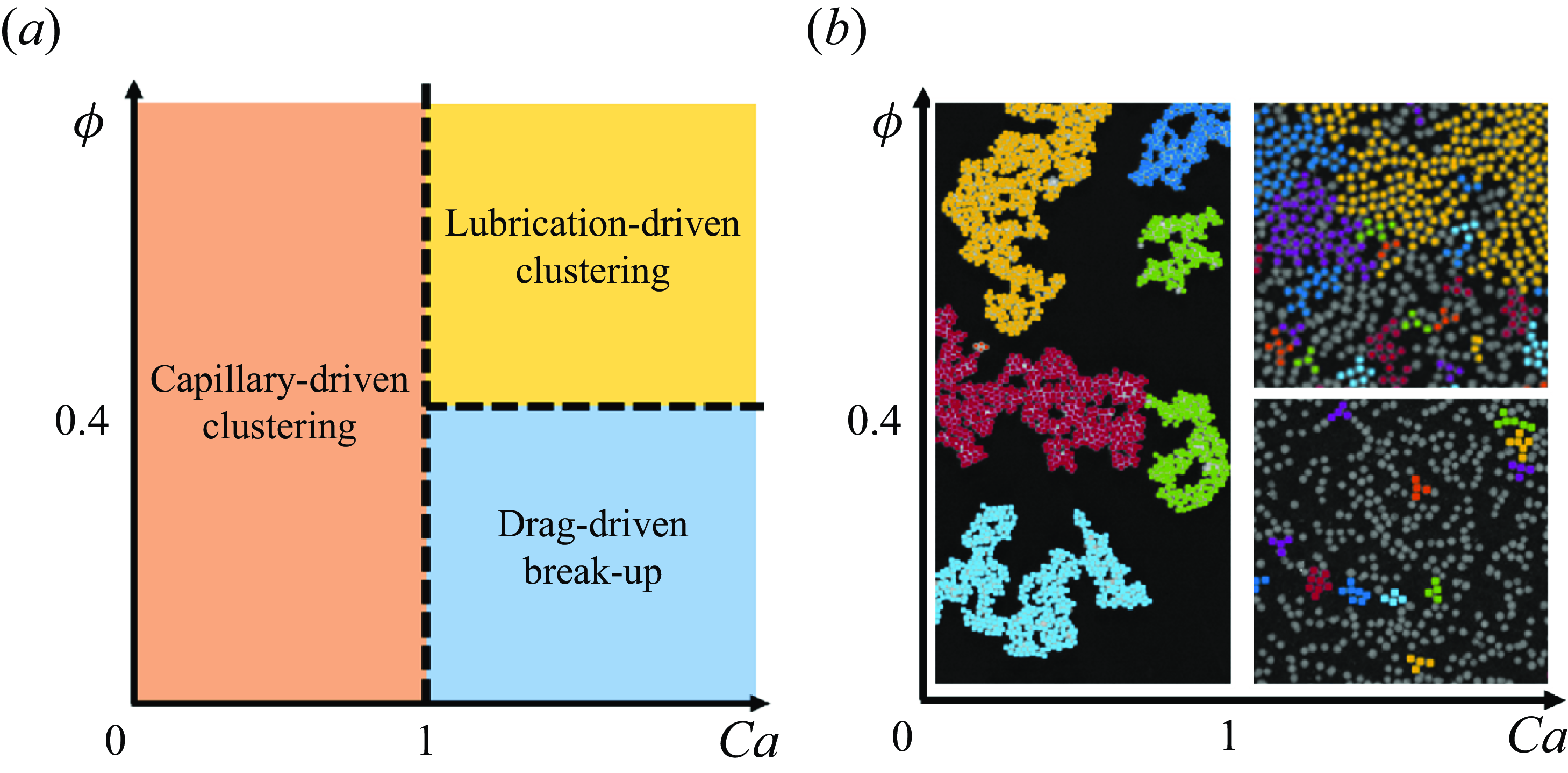
Figure 3. (a) Schematic of the three distinct clustering/break-up regimes within the $Ca-\phi$
phase space, adapted from Shin & Coletti (Reference Shin and Coletti2024). (b) Examples of detected clusters from each regime. Particles within the same cluster are indicated with the same colour.
$Ca-\phi$
phase space, adapted from Shin & Coletti (Reference Shin and Coletti2024). (b) Examples of detected clusters from each regime. Particles within the same cluster are indicated with the same colour.
3.1. Cluster properties
3.1.1. Clustering fraction and length scale
The fraction of particles forming clusters, denoted as $\chi _{cl}$
, is a key metric for understanding how the tendency to aggregating evolves across different flow regimes. This is defined as the number of particles contained in clusters, normalised by the total particle count. Figure 4(a) depicts
$\chi _{cl}$
, is a key metric for understanding how the tendency to aggregating evolves across different flow regimes. This is defined as the number of particles contained in clusters, normalised by the total particle count. Figure 4(a) depicts $\chi _{cl}$
as a function of
$\chi _{cl}$
as a function of $Ca$
at various
$Ca$
at various $\phi$
. As already discussed in Shin & Coletti (Reference Shin and Coletti2024),
$\phi$
. As already discussed in Shin & Coletti (Reference Shin and Coletti2024), $\chi _{cl}$
increases with decreasing
$\chi _{cl}$
increases with decreasing $Ca$
(as capillarity prevails over drag) and increasing
$Ca$
(as capillarity prevails over drag) and increasing $\phi$
(as lubrication prevails over drag). Moreover, for increasing
$\phi$
(as lubrication prevails over drag). Moreover, for increasing $Ca$
at a given
$Ca$
at a given $\phi$
,
$\phi$
, $\chi _{cl}$
approaches the level obtained in the synthetic data by RSA (dotted line). This implies that, when the fluid turbulence is sufficiently high, the statistical proximity of non-overlapping particles is largely responsible for the observed trend.
$\chi _{cl}$
approaches the level obtained in the synthetic data by RSA (dotted line). This implies that, when the fluid turbulence is sufficiently high, the statistical proximity of non-overlapping particles is largely responsible for the observed trend.
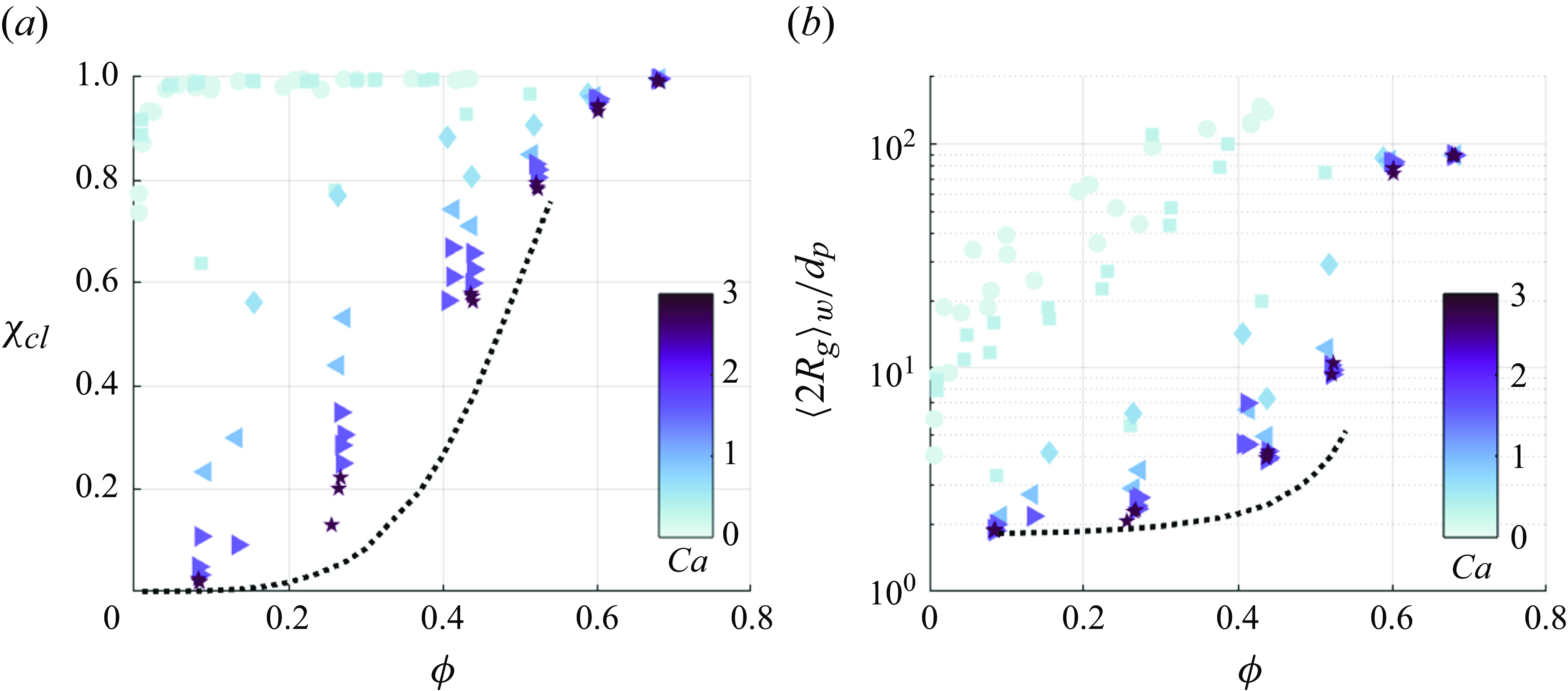
Figure 4. (a) Clustered particle fraction ( $\chi _{cl}$
) as a function of areal fraction (
$\chi _{cl}$
) as a function of areal fraction ( $\phi$
) across different capillary numbers (
$\phi$
) across different capillary numbers ( $Ca$
). (b) Normalised cluster size (
$Ca$
). (b) Normalised cluster size ( $\langle 2R_g \rangle _w/{d}_p$
) as a function of
$\langle 2R_g \rangle _w/{d}_p$
) as a function of $\phi$
at various
$\phi$
at various $Ca$
levels. In each case, the dotted line represents the clustering fractions from random configurations for the respective
$Ca$
levels. In each case, the dotted line represents the clustering fractions from random configurations for the respective $\phi$
values, established through RSA up to
$\phi$
values, established through RSA up to $\phi = 0.54$
.
$\phi = 0.54$
.
Figure 4(b) shows how the mean cluster length scale depends on $Ca$
and
$Ca$
and $\phi$
. To avoid biases induced by the large number of small clusters, we define the weighted-average radius as
$\phi$
. To avoid biases induced by the large number of small clusters, we define the weighted-average radius as
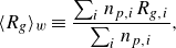 \begin{equation} \langle R_{g} \rangle _{w} \equiv \frac {\sum _{i} n_{p,i} R_{g,i}}{\sum _{i}n_{p,i}}, \end{equation}
where $R_{g,i}$
is the radius of gyration of the
$R_{g,i}$
is the radius of gyration of the $i$
th cluster and
$i$
th cluster and $n_{p,i}$
is the number of particles forming it. At low
$n_{p,i}$
is the number of particles forming it. At low $Ca$
, particles are heavily influenced by strong attractive capillary forces exceeding the disruptive effect of drag, leading to extended clusters. These can grow larger than a typical eddy size
$Ca$
, particles are heavily influenced by strong attractive capillary forces exceeding the disruptive effect of drag, leading to extended clusters. These can grow larger than a typical eddy size $L_F$
, comprising hundreds of particles. With increasing
$L_F$
, comprising hundreds of particles. With increasing $Ca$
, these objects have higher chance of being exposed to extensional strain exceeding the capillarity, leading to more frequent break-up and thus smaller aggregates. Again, with increasing
$Ca$
, these objects have higher chance of being exposed to extensional strain exceeding the capillarity, leading to more frequent break-up and thus smaller aggregates. Again, with increasing $Ca$
the radius obtained by RSA is approached. Overall, both
$Ca$
the radius obtained by RSA is approached. Overall, both $\chi _{cl}$
and
$\chi _{cl}$
and $\langle R_{g} \rangle _{w}$
indicate that, when the turbulent forcing is intense and
$\langle R_{g} \rangle _{w}$
indicate that, when the turbulent forcing is intense and $Ca \gg 1$
, the clustering is increasingly governed by the stochastic adjacency of particles, rather than inter-particle interactions.
$Ca \gg 1$
, the clustering is increasingly governed by the stochastic adjacency of particles, rather than inter-particle interactions.
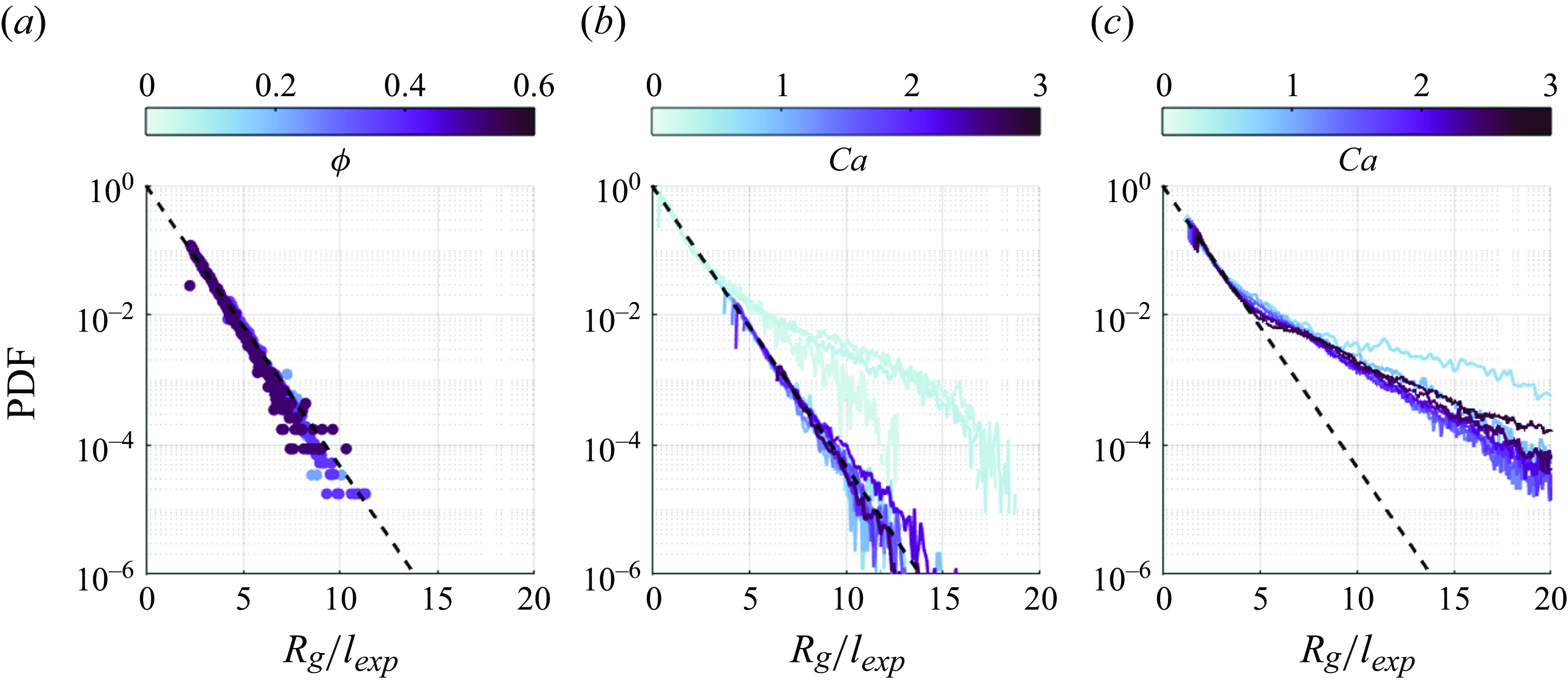
Figure 5. Probability density functions (PDFs) of the cluster size, $R_g$
, normalised by the exponential decay length, (
$R_g$
, normalised by the exponential decay length, ( $l_{exp }$
): (a) RSA-generated random configurations at
$l_{exp }$
): (a) RSA-generated random configurations at $\phi = 0.27$
, 0.44 and 0.53. The corresponding values of
$\phi = 0.27$
, 0.44 and 0.53. The corresponding values of $l_{exp }/{d}_p$
are 0.20, 0.33 and 0.87, respectively. (b) The PDFs at
$l_{exp }/{d}_p$
are 0.20, 0.33 and 0.87, respectively. (b) The PDFs at $\phi = 0.27$
for various experimental capillary numbers:
$\phi = 0.27$
for various experimental capillary numbers: $Ca= 0.16$
, 0.23, 0.29, 0.87, 1.22, 1.51, 1.82, 2.10, 2.49 and 2.69, with the corresponding values of
$Ca= 0.16$
, 0.23, 0.29, 0.87, 1.22, 1.51, 1.82, 2.10, 2.49 and 2.69, with the corresponding values of $l_{exp }/{d}_p= 5.66$
, 4.16, 3.76, 0.41, 0.37, 0.33, 0.29, 0.32, 0.25 and 0.21, respectively. (c) The PDFs at
$l_{exp }/{d}_p= 5.66$
, 4.16, 3.76, 0.41, 0.37, 0.33, 0.29, 0.32, 0.25 and 0.21, respectively. (c) The PDFs at $\phi =0.53$
for
$\phi =0.53$
for $Ca = 0.59$
, 0.87, 1.22, 1.51, 1.82, 2.10, 2.49 and 2.69 with the corresponding values of
$Ca = 0.59$
, 0.87, 1.22, 1.51, 1.82, 2.10, 2.49 and 2.69 with the corresponding values of $l_{exp }= 1.17$
, 1.00, 1.00, 0.95, 0.88, 0.83, 0.79 and 0.74. The black dashed line in each panel represents an exponential decay,
$l_{exp }= 1.17$
, 1.00, 1.00, 0.95, 0.88, 0.83, 0.79 and 0.74. The black dashed line in each panel represents an exponential decay, $\exp (-R_g/l_{exp })$
.
$\exp (-R_g/l_{exp })$
.
The PDFs of $R_{g}$
offer further insight into how the clustering dynamics changes across regimes. Figure 5(a) shows that clusters formed by RSA exhibit an exponential distribution, independently of
$R_{g}$
offer further insight into how the clustering dynamics changes across regimes. Figure 5(a) shows that clusters formed by RSA exhibit an exponential distribution, independently of $\phi$
. An exponential fit of the probability
$\phi$
. An exponential fit of the probability $p(R_g) \sim \exp (-R_g / l_{exp })$
, applied to the RSA data as well as to experimental data that exhibit exponential decay, defines a characteristic length
$p(R_g) \sim \exp (-R_g / l_{exp })$
, applied to the RSA data as well as to experimental data that exhibit exponential decay, defines a characteristic length $l_{exp }$
used to normalise the distributions in the different scenarios. Moderately dense systems (figure 5
b) exhibit a transition with varying
$l_{exp }$
used to normalise the distributions in the different scenarios. Moderately dense systems (figure 5
b) exhibit a transition with varying $Ca$
: in the capillary-driven clustering regime (
$Ca$
: in the capillary-driven clustering regime ( $Ca \lt 1$
) the cluster radius PDFs possess long tails, with significant probability of large aggregates spanning the entire domain; while in the drag-driven break-up regime (
$Ca \lt 1$
) the cluster radius PDFs possess long tails, with significant probability of large aggregates spanning the entire domain; while in the drag-driven break-up regime ( $Ca \gt 1, \phi \lt 0.40$
) drag disrupts the large clusters and the distribution gradually approaches the RSA behaviour. This observation supports the view that the clustering dynamics in moderately dilute systems is predominantly influenced by the random proximity of particles.
$Ca \gt 1, \phi \lt 0.40$
) drag disrupts the large clusters and the distribution gradually approaches the RSA behaviour. This observation supports the view that the clustering dynamics in moderately dilute systems is predominantly influenced by the random proximity of particles.
The scenario is different for denser systems (figure 5
c). Here, both in the capillarity-driven regime ( $Ca \lt 1$
) and in the lubrication-driven clustering regime (
$Ca \lt 1$
) and in the lubrication-driven clustering regime ( $Ca \gt 1, \phi \gt 0.40$
), the decay of the PDFs is much slower compared with RSA. This implies that the formation of very large clusters cannot be explained by excluded volume effect at high concentration, and are instead sustained by lubrication forces. At even higher concentrations, few large clusters percolate through the whole system. This scenario is discussed in the next section.
$Ca \gt 1, \phi \gt 0.40$
), the decay of the PDFs is much slower compared with RSA. This implies that the formation of very large clusters cannot be explained by excluded volume effect at high concentration, and are instead sustained by lubrication forces. At even higher concentrations, few large clusters percolate through the whole system. This scenario is discussed in the next section.
3.1.2. Cluster percolation and self-similarity
Dense particle systems are known to exhibit sharp transitions to a percolating state when their concentration increases above a threshold. In such a state, exceptionally large clusters are formed that span the entire domain. The threshold is system-dependent: for example, Shen, O’Hern & Shattuck (Reference Shen, O’Hern and Shattuck2012) found a critical area fraction $\phi ^{*}=0.549$
by simulating periodic 2-D layers of frictionless particles under compression, while the experiments of Alicke, Stricker & Vermant (Reference Alicke, Stricker and Vermant2023) found
$\phi ^{*}=0.549$
by simulating periodic 2-D layers of frictionless particles under compression, while the experiments of Alicke, Stricker & Vermant (Reference Alicke, Stricker and Vermant2023) found $\phi ^{*}=0.3-0.36$
for particle layers under shear and compression.
$\phi ^{*}=0.3-0.36$
for particle layers under shear and compression.
The present system also exhibits a transition to a percolating state. This is illustrated in figures 6(a) and 6(b), where instantaneous realisations are shown for two representative cases at $Ca = 0.33$
. While both have comparable concentrations
$Ca = 0.33$
. While both have comparable concentrations $\phi = 0.44$
and
$\phi = 0.44$
and $0.53$
, only the latter displays percolating clusters. The transition is quantified in figure 6(c), plotting the percolation fraction
$0.53$
, only the latter displays percolating clusters. The transition is quantified in figure 6(c), plotting the percolation fraction $\chi _p$
(number of imaging frames featuring at least one cluster percolating through the whole field of view, divided by the total number of acquired frames) as a function of
$\chi _p$
(number of imaging frames featuring at least one cluster percolating through the whole field of view, divided by the total number of acquired frames) as a function of $\phi$
, for a representative value of
$\phi$
, for a representative value of $Ca=0.33$
. While we do not vary
$Ca=0.33$
. While we do not vary $\phi$
finely enough to identify a precise threshold
$\phi$
finely enough to identify a precise threshold $\phi ^{*}$
, the transition appears relatively sharp. Visual inspection also confirms that the formation of a percolation cluster is hindered by increasing
$\phi ^{*}$
, the transition appears relatively sharp. Visual inspection also confirms that the formation of a percolation cluster is hindered by increasing $Ca$
, which favours more homogeneous patterns (figure 6
d).
$Ca$
, which favours more homogeneous patterns (figure 6
d).
The trend across the parameter space is summarised in figure 6(e). For $Ca \ll 1$
, we estimate
$Ca \ll 1$
, we estimate $\phi ^{*} \sim 0.4 - 0.5$
, comparable to classic configurations of compressed/sheared particle layers (Alicke et al. Reference Alicke, Stricker and Vermant2023). On the other hand, for
$\phi ^{*} \sim 0.4 - 0.5$
, comparable to classic configurations of compressed/sheared particle layers (Alicke et al. Reference Alicke, Stricker and Vermant2023). On the other hand, for $Ca \geqslant 1$
, the threshold is significantly higher,
$Ca \geqslant 1$
, the threshold is significantly higher, $\phi ^{*} \sim 0.55 - 0.6$
. This is consistent with the notion that percolation naturally emerges in self-similar systems, where the influence of a preferential scale characterising the pattern is weak or absent (Aharony & Stauffer Reference Aharony and Stauffer2003). At large
$\phi ^{*} \sim 0.55 - 0.6$
. This is consistent with the notion that percolation naturally emerges in self-similar systems, where the influence of a preferential scale characterising the pattern is weak or absent (Aharony & Stauffer Reference Aharony and Stauffer2003). At large $Ca$
, the flow increasingly imposes the forcing length scale
$Ca$
, the flow increasingly imposes the forcing length scale $L_F$
that disrupts system-spanning clusters, and percolation can only be attained at the largest concentrations. In particular, as we showed in Shin & Coletti (Reference Shin and Coletti2024), for
$L_F$
that disrupts system-spanning clusters, and percolation can only be attained at the largest concentrations. In particular, as we showed in Shin & Coletti (Reference Shin and Coletti2024), for $Ca\gt 1$
, the typical cluster size exceeds
$Ca\gt 1$
, the typical cluster size exceeds $L_{F}$
only for areal fractions above
$L_{F}$
only for areal fractions above $\phi \sim 0.55$
(which we now identify as the approximate percolation threshold in this regime).
$\phi \sim 0.55$
(which we now identify as the approximate percolation threshold in this regime).
The dominant role of the forcing scale, as opposed to the larger scales where energy accumulates in Q2-D turbulence, was already stressed in studies of Lagrangian dispersion (Xia et al. Reference Xia, Francois, Punzmann and Shats2013, Reference Xia, Francois, Punzmann and Shats2019). For both particle clustering and dispersion, such a role is likely rooted in the persistent nature of eddies of size $L_F$
(see discussion in Xia et al. Reference Xia, Francois, Punzmann and Shats2013). On the other hand, when inter-particle attraction becomes dominant, cohesive clusters much larger than
$L_F$
(see discussion in Xia et al. Reference Xia, Francois, Punzmann and Shats2013). On the other hand, when inter-particle attraction becomes dominant, cohesive clusters much larger than $L_F$
appear. One may hypothesise that those might be related to commensurately large-scale fluid motions, either due to the inverse cascade or engendered by the influence of the clusters themselves on the flow. To investigate this possibility, we define the Eulerian velocity autocorrelation
$L_F$
appear. One may hypothesise that those might be related to commensurately large-scale fluid motions, either due to the inverse cascade or engendered by the influence of the clusters themselves on the flow. To investigate this possibility, we define the Eulerian velocity autocorrelation $\Gamma _E(r)=\langle \boldsymbol{u}(\boldsymbol{x}_0,t) \cdot \boldsymbol{u}(\boldsymbol{x}_0 + \boldsymbol{r},t) \rangle _{\boldsymbol{x}_0,t} / \langle \boldsymbol{u}(\boldsymbol{x}_0,t) \cdot \boldsymbol{u}(\boldsymbol{x}_0,t) \rangle _{\boldsymbol{x}_0,t}$
and compare it for both particles and tracers. This is shown in figure 7 for the representative case
$\Gamma _E(r)=\langle \boldsymbol{u}(\boldsymbol{x}_0,t) \cdot \boldsymbol{u}(\boldsymbol{x}_0 + \boldsymbol{r},t) \rangle _{\boldsymbol{x}_0,t} / \langle \boldsymbol{u}(\boldsymbol{x}_0,t) \cdot \boldsymbol{u}(\boldsymbol{x}_0,t) \rangle _{\boldsymbol{x}_0,t}$
and compare it for both particles and tracers. This is shown in figure 7 for the representative case $Ca=2.69$
and
$Ca=2.69$
and $\phi =0.62$
. It highlights how, even when particles form large percolating clusters, the correlation scale of their motion matches that of the fluid flow (approximately
$\phi =0.62$
. It highlights how, even when particles form large percolating clusters, the correlation scale of their motion matches that of the fluid flow (approximately $0.5L_F$
, see Shin et al. Reference Shin, Coletti and Conlin2023). We deduce that the emergence of system-spanning clusters is not related to fluid motions at scales larger than
$0.5L_F$
, see Shin et al. Reference Shin, Coletti and Conlin2023). We deduce that the emergence of system-spanning clusters is not related to fluid motions at scales larger than $L_F$
.
$L_F$
.
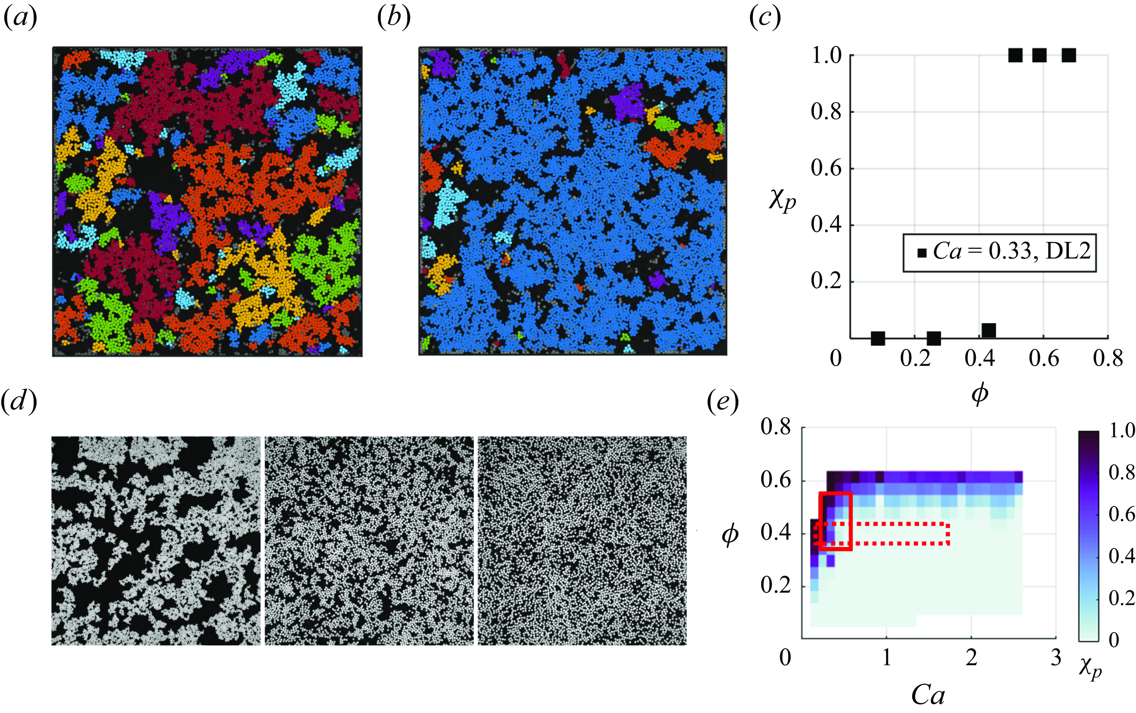
Figure 6. Snapshots with identified clusters at the same $Ca = 0.33$
but different areal fractions: (a)
$Ca = 0.33$
but different areal fractions: (a) $\phi = 0.44$
, and (b)
$\phi = 0.44$
, and (b) $\phi = 0.53$
. Particles within the same cluster are indicated with the same colour. (c) Fraction of frames
$\phi = 0.53$
. Particles within the same cluster are indicated with the same colour. (c) Fraction of frames $\chi _p$
where a system-spanning cluster is present as a function of
$\chi _p$
where a system-spanning cluster is present as a function of $\phi$
at fixed
$\phi$
at fixed $Ca = 0.33$
. (d) Examples of cluster morphology for systems with
$Ca = 0.33$
. (d) Examples of cluster morphology for systems with $\phi \approx 0.44$
at different capillary numbers:
$\phi \approx 0.44$
at different capillary numbers: $Ca = 0.29$
, 0.59 and 1.82 (from left to right). At this
$Ca = 0.29$
, 0.59 and 1.82 (from left to right). At this $\phi$
,
$\phi$
, $Ca \ll 1$
entails the formation of a percolating structure, while higher
$Ca \ll 1$
entails the formation of a percolating structure, while higher $Ca$
results in non-connected structures. (e) Value of
$Ca$
results in non-connected structures. (e) Value of $\chi _p$
in the
$\chi _p$
in the $Ca-\phi$
space. Panels (a) and (b) correspond to the points inside the red solid rectangle, and panel (d) corresponds to cases inside the red dotted rectangle.
$Ca-\phi$
space. Panels (a) and (b) correspond to the points inside the red solid rectangle, and panel (d) corresponds to cases inside the red dotted rectangle.
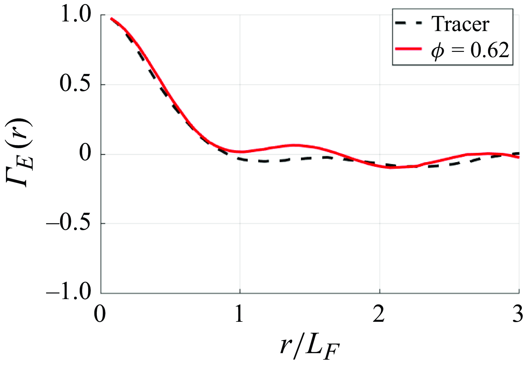
Figure 7. Examples of the Eulerian velocity autocorrelation for the DL configuration. The dashed line represents tracers ( $Re=1047$
), while the red line corresponds to a dense suspension of particles at the same level of forcing (
$Re=1047$
), while the red line corresponds to a dense suspension of particles at the same level of forcing ( $Ca=2.69$
and
$Ca=2.69$
and $\phi =0.62$
), where they form a large, system-spanning cluster.
$\phi =0.62$
), where they form a large, system-spanning cluster.
In order to further characterise the present system within the percolation framework, we analyse the cluster size distributions. Unlike in sub-§ 3.1.1 where we focused on a geometric scale, here, we focus on the size, intended as the number of particles $n_p$
contained in each cluster. In particular, we evaluate the cluster number density
$n_p$
contained in each cluster. In particular, we evaluate the cluster number density $f(n_p)$
, namely the number density of clusters of size
$f(n_p)$
, namely the number density of clusters of size $n_p$
per unit area. In 2-D self-similar particle systems (e.g. patterns of droplets condensing on surfaces (Stricker et al. Reference Stricker, Grillo, Marquez, Panzarasa, Smith-Mannschott and Vollmer2022), we expect
$n_p$
per unit area. In 2-D self-similar particle systems (e.g. patterns of droplets condensing on surfaces (Stricker et al. Reference Stricker, Grillo, Marquez, Panzarasa, Smith-Mannschott and Vollmer2022), we expect $f(n_p) \sim (n_p/n_{p,max})^{-\xi }(n_{p,max} A_p)^{-\theta }$
, where
$f(n_p) \sim (n_p/n_{p,max})^{-\xi }(n_{p,max} A_p)^{-\theta }$
, where $n_{p,max}$
is the size of the largest cluster in the distribution,
$n_{p,max}$
is the size of the largest cluster in the distribution, $\xi$
is the so-called polydispersity exponent characterising the scaling range,
$\xi$
is the so-called polydispersity exponent characterising the scaling range, $A_p=\pi {d}_p^{2}/4$
is the projected area of a particle and
$A_p=\pi {d}_p^{2}/4$
is the projected area of a particle and $\theta$
is a trivial exponent depending on the dimensionality of the system, which has here the value of 1 to guarantee dimensional consistency.
$\theta$
is a trivial exponent depending on the dimensionality of the system, which has here the value of 1 to guarantee dimensional consistency.
Figure 8(a) reports $f(n_p)$
for cases of comparable areal fraction,
$f(n_p)$
for cases of comparable areal fraction, $\phi \sim 0.44$
, displaying self-similar scaling ranges with a polydispersity exponent that varies with
$\phi \sim 0.44$
, displaying self-similar scaling ranges with a polydispersity exponent that varies with $Ca$
(considering comparable or higher concentrations, not shown for brevity, leads to analogous conclusions). To extract the polydispersity exponents, we rescale
$Ca$
(considering comparable or higher concentrations, not shown for brevity, leads to analogous conclusions). To extract the polydispersity exponents, we rescale $f(n_p)$
in figure 8 to have
$f(n_p)$
in figure 8 to have $f(n_p)(n_{p,max}A_p)^{\theta }$
, which is expected to scale as
$f(n_p)(n_{p,max}A_p)^{\theta }$
, which is expected to scale as $(n_p/n_{p,max})^{-\xi }$
.
$(n_p/n_{p,max})^{-\xi }$
.

Figure 8. (a) Cluster size distributions for a particle area fraction $\phi \approx 0.44$
at different capillary numbers
$\phi \approx 0.44$
at different capillary numbers $Ca$
. Here,
$Ca$
. Here, $n_p$
is the number of particles within a cluster, characterising the cluster size and
$n_p$
is the number of particles within a cluster, characterising the cluster size and $f(n_p)$
is the areal number density of clusters of size
$f(n_p)$
is the areal number density of clusters of size $n_p$
. Dashed lines denote experiments in the SL configuration, while solid lines are from the DL2 set-up. (b) Normalised form of the same data, where
$n_p$
. Dashed lines denote experiments in the SL configuration, while solid lines are from the DL2 set-up. (b) Normalised form of the same data, where $n_{p,max}$
is the size of the largest cluster,
$n_{p,max}$
is the size of the largest cluster, $A_p = \pi {d}_p^{2}/4$
is the projected area of a particle and
$A_p = \pi {d}_p^{2}/4$
is the projected area of a particle and $\theta = 1$
is a trivial exponent from dimensional analysis. Two limiting values of the polydispersity exponents,
$\theta = 1$
is a trivial exponent from dimensional analysis. Two limiting values of the polydispersity exponents, $\xi =2.05$
(dash-dot) and
$\xi =2.05$
(dash-dot) and $\xi =5/2$
(dotted), which correspond to the predicted Fisher’s exponent (Fisher Reference Fisher1967), are indicated.
$\xi =5/2$
(dotted), which correspond to the predicted Fisher’s exponent (Fisher Reference Fisher1967), are indicated.
For $Ca \lt 1$
, the scaling range is broad and
$Ca \lt 1$
, the scaling range is broad and $\xi$
is somewhat smaller than but comparable to the value of 2.05 characterising 2-D percolation, as observed in randomly generated clusters on regular lattices (Stauffer Reference Stauffer1979). The discrepancy may be attributed to finite size effects.
$\xi$
is somewhat smaller than but comparable to the value of 2.05 characterising 2-D percolation, as observed in randomly generated clusters on regular lattices (Stauffer Reference Stauffer1979). The discrepancy may be attributed to finite size effects.
This indicates that, in the capillary-driven clustering regime, the present system shares similarities (at least topologically) with classic percolating particle systems. For large capillary numbers $Ca \gt 1$
, on the other hand, the scaling range is narrower as the forcing hinders the formation of self-similar structures. Over approximately a decade, however, the size distribution is consistent with a polydispersity exponent
$Ca \gt 1$
, on the other hand, the scaling range is narrower as the forcing hinders the formation of self-similar structures. Over approximately a decade, however, the size distribution is consistent with a polydispersity exponent $\xi = 5/2$
. This corresponds to the well-known prediction derived by Fisher (Reference Fisher1967) for a coagulation process under the assumption that each agglomerate has equal probability of interacting with any other. Such a condition is typically not satisfied in standard percolation processes, leading to shallower exponents (Hoshent et al. Reference Hoshent, Stauffer, Bishop, Harrison and Quinn1979; Stauffer Reference Stauffer1979). We therefore hypothesise that, in the present configuration, the forcing by the underlying turbulence contributes to randomising the system, effectively restoring the validity of Fisher’s assumption. We remark that this is the first observation of a percolation transition in turbulent particle suspensions, and its detailed properties deserve further investigation.
$\xi = 5/2$
. This corresponds to the well-known prediction derived by Fisher (Reference Fisher1967) for a coagulation process under the assumption that each agglomerate has equal probability of interacting with any other. Such a condition is typically not satisfied in standard percolation processes, leading to shallower exponents (Hoshent et al. Reference Hoshent, Stauffer, Bishop, Harrison and Quinn1979; Stauffer Reference Stauffer1979). We therefore hypothesise that, in the present configuration, the forcing by the underlying turbulence contributes to randomising the system, effectively restoring the validity of Fisher’s assumption. We remark that this is the first observation of a percolation transition in turbulent particle suspensions, and its detailed properties deserve further investigation.
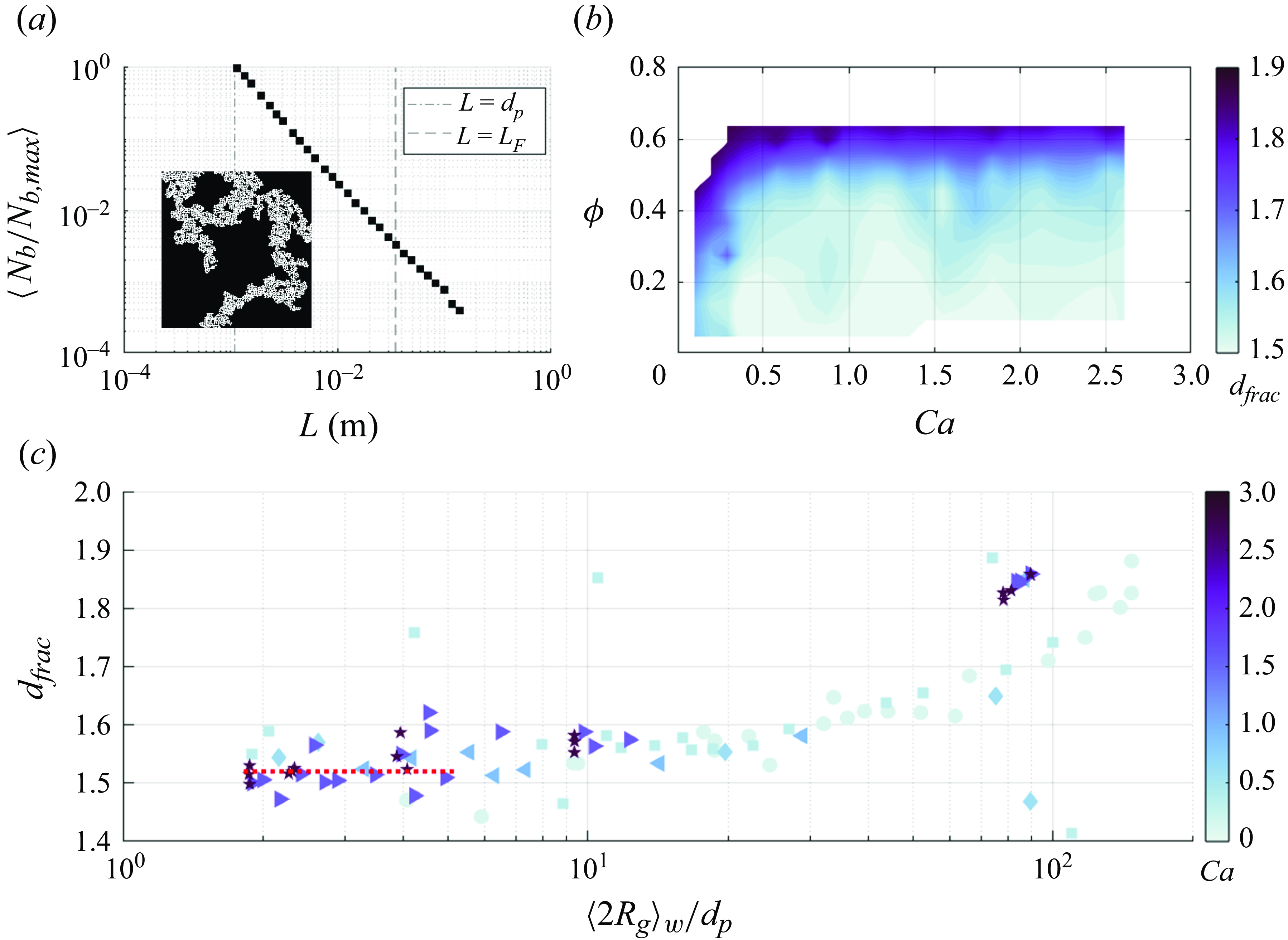
Figure 9. Fractal dimension $d_{frac}$
obtained via the box-counting method. (a) An example of normalised box count as a function of box side length for a cluster (inset), (b)
$d_{frac}$
obtained via the box-counting method. (a) An example of normalised box count as a function of box side length for a cluster (inset), (b) $d_{frac}$
mapped in the
$d_{frac}$
mapped in the $Ca-\phi$
space and (c)
$Ca-\phi$
space and (c) $d_{frac}$
as a function of the mean cluster size. The red dotted line indicates the mean
$d_{frac}$
as a function of the mean cluster size. The red dotted line indicates the mean $d_{frac}$
from varying
$d_{frac}$
from varying $\phi$
values obtained via RSA.
$\phi$
values obtained via RSA.
3.1.3. Clusters’ internal structure
The different mechanisms at play in the $Ca-\phi$
space can affect not only the clusters’ size but also their internal structure. Even though particle patterns may not be strictly self-similar, an operational definition of fractal dimension
$Ca-\phi$
space can affect not only the clusters’ size but also their internal structure. Even though particle patterns may not be strictly self-similar, an operational definition of fractal dimension $d_{frac}$
can be useful to quantify the compactness and complexity of their geometry. To estimate it, we select in each frame the cluster containing the largest number of particles, and we reconstruct its binary image based on the centroids and diameter of its particles. We then apply to it the box-counting method (Monchaux, Bourgoin & Cartellier Reference Monchaux, Bourgoin and Cartellier2012; Baker et al. Reference Baker, Frankel, Mani and Coletti2017), with
$d_{frac}$
can be useful to quantify the compactness and complexity of their geometry. To estimate it, we select in each frame the cluster containing the largest number of particles, and we reconstruct its binary image based on the centroids and diameter of its particles. We then apply to it the box-counting method (Monchaux, Bourgoin & Cartellier Reference Monchaux, Bourgoin and Cartellier2012; Baker et al. Reference Baker, Frankel, Mani and Coletti2017), with $L$
the box size (figure 9
a). The data are normalised by the maximum count
$L$
the box size (figure 9
a). The data are normalised by the maximum count $N_{b,max}$
obtained from the smallest box size (
$N_{b,max}$
obtained from the smallest box size ( $L=O({d}_p)$
) yielding a plot of
$L=O({d}_p)$
) yielding a plot of $N_b / N_{b,max}$
as a function of
$N_b / N_{b,max}$
as a function of $L$
, where
$L$
, where $N_b$
is the number of boxes that cover the binarised cluster. The normalised curves from all analysed clusters are averaged to extract
$N_b$
is the number of boxes that cover the binarised cluster. The normalised curves from all analysed clusters are averaged to extract $d_{frac}$
by linear fitting in logarithmic scale.
$d_{frac}$
by linear fitting in logarithmic scale.
Figure 9(b) maps the fractal dimension in the $Ca-\phi$
space. Similarly to
$Ca-\phi$
space. Similarly to $\chi _{cl}$
and
$\chi _{cl}$
and $\langle R_g \rangle _w$
previously discussed,
$\langle R_g \rangle _w$
previously discussed, $d_{frac}$
drops sharply in moderately dense suspensions (
$d_{frac}$
drops sharply in moderately dense suspensions ( $\phi \lt 0.40$
) within a narrow range of
$\phi \lt 0.40$
) within a narrow range of $Ca\lt 1$
. Further increasing
$Ca\lt 1$
. Further increasing $Ca$
leads to
$Ca$
leads to $d_{frac}$
flattening around 1.5, close to the baseline value of
$d_{frac}$
flattening around 1.5, close to the baseline value of $1.52 \pm 0.2$
from RSA which exhibits negligible
$1.52 \pm 0.2$
from RSA which exhibits negligible $\phi$
dependence. When
$\phi$
dependence. When $Ca \gt 1$
, the contour lines become largely horizontal, signalling a major role of
$Ca \gt 1$
, the contour lines become largely horizontal, signalling a major role of $\phi$
. The lubrication-driven clusters are indeed compact, the particles filling the open spaces in their internal structure.
$\phi$
. The lubrication-driven clusters are indeed compact, the particles filling the open spaces in their internal structure.
We now consider how $d_{frac}$
varies with
$d_{frac}$
varies with $\langle R_{g} \rangle _w$
(figure 9
c). While small clusters (up to
$\langle R_{g} \rangle _w$
(figure 9
c). While small clusters (up to $\langle R_g \rangle _w / {d}_p = O(10)$
) exhibit values of
$\langle R_g \rangle _w / {d}_p = O(10)$
) exhibit values of $d_{frac}$
similar to those generated by RSA, for larger ones
$d_{frac}$
similar to those generated by RSA, for larger ones $d_{frac}$
increases with size, tending to (although never reaching) the value of 2 characteristic of round (non-fractal) objects. For large
$d_{frac}$
increases with size, tending to (although never reaching) the value of 2 characteristic of round (non-fractal) objects. For large $\langle R_g \rangle _w / {d}_p = O(10^{2})$
,
$\langle R_g \rangle _w / {d}_p = O(10^{2})$
, $d_{frac}$
is significantly lower for
$d_{frac}$
is significantly lower for $Ca \lt 1$
. This indicates a convoluted structure, which can be the result of hit-and-stick collisions, frequent when the capillary forces are too strong to be overcome by drag. In contrast, clusters at
$Ca \lt 1$
. This indicates a convoluted structure, which can be the result of hit-and-stick collisions, frequent when the capillary forces are too strong to be overcome by drag. In contrast, clusters at $Ca\gt 1$
have a more dynamic composition, with particles continuously joining and leaving the aggregate due to relatively weaker cohesive forces. Thus, we can draw an analogy between the cluster formation at low
$Ca\gt 1$
have a more dynamic composition, with particles continuously joining and leaving the aggregate due to relatively weaker cohesive forces. Thus, we can draw an analogy between the cluster formation at low $Ca$
and the diffusion-limited cluster aggregation (DLCA) which is known to result in more open (less compact) clusters (Meakin Reference Meakin1983; Lazzari et al. Reference Lazzari, Nicoud, Jaquet, Lattuada and Morbidelli2016). Notably, unlike DLCA of colloids driven by Brownian diffusion, our system employs non-Brownian particles driven by the underlying turbulent flow. In systems exhibiting aggregation of particles in turbulence, the fractal dimension of the aggregates has been evaluated both experimentally (e.g. Maggi, Mietta & Winterwerp Reference Maggi, Mietta and Winterwerp2007) and numerically (e.g. Zhao et al. Reference Zhao, Pomes, Vowinckel, Hsu, Bai and Meiburg2021). In particular, Zhao et al. (Reference Zhao, Pomes, Vowinckel, Hsu, Bai and Meiburg2021) provided empirical scaling for
$Ca$
and the diffusion-limited cluster aggregation (DLCA) which is known to result in more open (less compact) clusters (Meakin Reference Meakin1983; Lazzari et al. Reference Lazzari, Nicoud, Jaquet, Lattuada and Morbidelli2016). Notably, unlike DLCA of colloids driven by Brownian diffusion, our system employs non-Brownian particles driven by the underlying turbulent flow. In systems exhibiting aggregation of particles in turbulence, the fractal dimension of the aggregates has been evaluated both experimentally (e.g. Maggi, Mietta & Winterwerp Reference Maggi, Mietta and Winterwerp2007) and numerically (e.g. Zhao et al. Reference Zhao, Pomes, Vowinckel, Hsu, Bai and Meiburg2021). In particular, Zhao et al. (Reference Zhao, Pomes, Vowinckel, Hsu, Bai and Meiburg2021) provided empirical scaling for $d_{frac}$
as a function of the key non-dimensional parameters. The present results qualitatively agree with their model, e.g. concerning the increase of
$d_{frac}$
as a function of the key non-dimensional parameters. The present results qualitatively agree with their model, e.g. concerning the increase of $d_{frac}$
with larger cluster size. A quantitative comparison, however, is hindered by the fact that the present configuration is quasi-two-dimensional.
$d_{frac}$
with larger cluster size. A quantitative comparison, however, is hindered by the fact that the present configuration is quasi-two-dimensional.
A natural metric to assess the degree of ordering/packing inside clusters is the hexatic order parameter $\psi _{6}$
, which measures the local ordering based on the orientation of the particle’s six nearest neighbours. For the particle
$\psi _{6}$
, which measures the local ordering based on the orientation of the particle’s six nearest neighbours. For the particle $j$
, it is defined as
$j$
, it is defined as
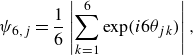 \begin{equation} \psi _{6,j} = \frac {1}{6}\left |\sum _{k=1}^{6}\exp (i6\theta _{jk})\right |, \end{equation}
where $k$
is an index for the six nearest neighbouring particles,
$k$
is an index for the six nearest neighbouring particles, $\theta _{jk}$
is the angle between the reference direction and the line connecting the particle
$\theta _{jk}$
is the angle between the reference direction and the line connecting the particle $j$
and its neighbouring particle
$j$
and its neighbouring particle $k$
.
$k$
.
We assess $\psi _6$
for all individual clustered particles, ranging between 0 (dislocations and disclinations) and 1 (hexagonal crystal). Figure 10(a) compares the PDFs of
$\psi _6$
for all individual clustered particles, ranging between 0 (dislocations and disclinations) and 1 (hexagonal crystal). Figure 10(a) compares the PDFs of $\psi _6$
for the same
$\psi _6$
for the same $\phi =0.44$
and two different
$\phi =0.44$
and two different $Ca$
. It is clear that lower
$Ca$
. It is clear that lower $Ca$
yields higher probabilities of large
$Ca$
yields higher probabilities of large $\psi _6$
values. Increasing
$\psi _6$
values. Increasing $Ca$
pushes the PDF towards lower
$Ca$
pushes the PDF towards lower $\psi _6$
values, approaching the distribution obtained by RSA at the corresponding area fraction.
$\psi _6$
values, approaching the distribution obtained by RSA at the corresponding area fraction.
We further consider the average hexatic order parameter over all clustered particles, $\langle \psi _6 \rangle$
, in the
$\langle \psi _6 \rangle$
, in the $Ca-\phi$
space (figure 10
b). This displays a similar trend to previously discussed metrics: it diminishes as the system transitions from the capillary-driven clustering to drag-driven regime, and increases transitioning to lubrication-driven clustering. Plotting
$Ca-\phi$
space (figure 10
b). This displays a similar trend to previously discussed metrics: it diminishes as the system transitions from the capillary-driven clustering to drag-driven regime, and increases transitioning to lubrication-driven clustering. Plotting $\langle \psi _6 \rangle$
as a function of
$\langle \psi _6 \rangle$
as a function of $\phi$
(figure 10
c) indicates how the high-
$\phi$
(figure 10
c) indicates how the high- $Ca$
cases follow closely the values obtained by RSA. This indicates again that clusters formed under strong turbulence forcing tend to resemble those formed by a random process.
$Ca$
cases follow closely the values obtained by RSA. This indicates again that clusters formed under strong turbulence forcing tend to resemble those formed by a random process.
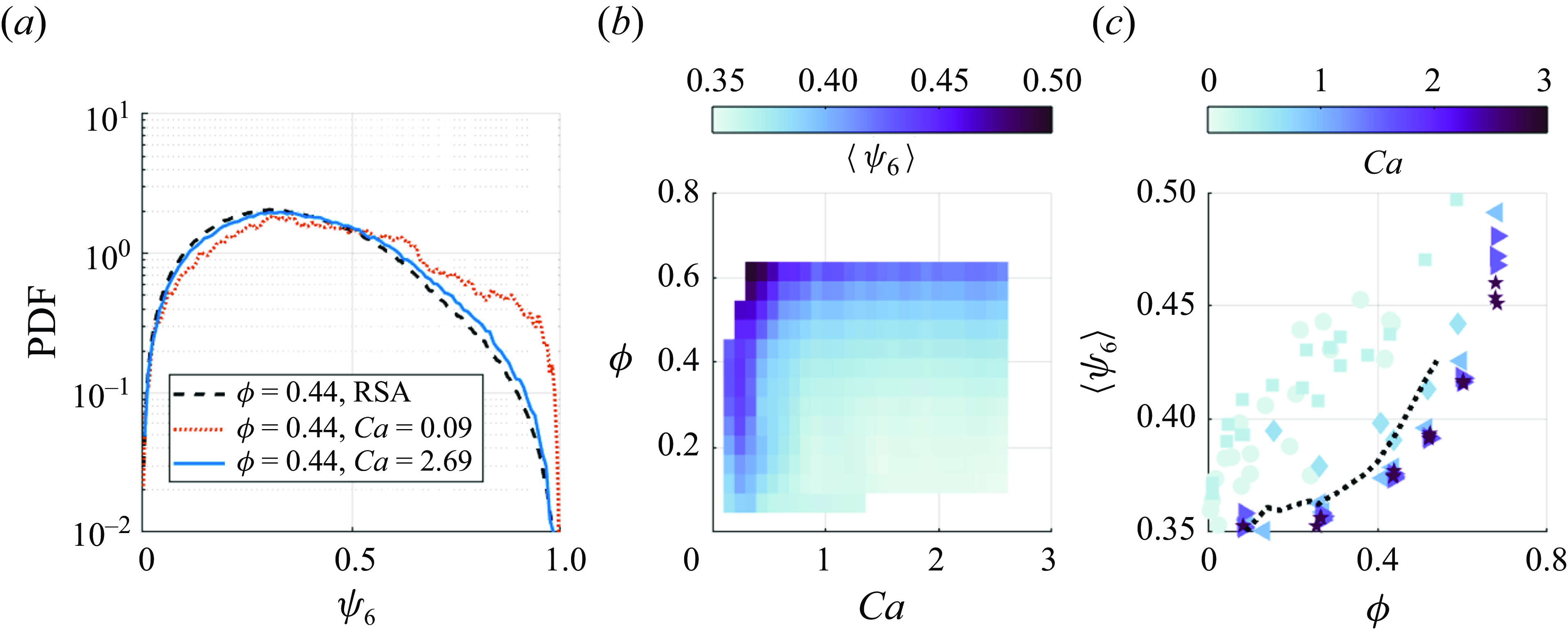
Figure 10. Hexatic order parameter ( $\psi _6$
) of the clustered particles. (a) The PDFs of
$\psi _6$
) of the clustered particles. (a) The PDFs of $\psi _6$
at
$\psi _6$
at $\phi = 0.44$
but different
$\phi = 0.44$
but different $Ca$
values: 0.09 (red) and 2.69 (blue). The black dashed line represents values from RSA for comparison. (b) Value of
$Ca$
values: 0.09 (red) and 2.69 (blue). The black dashed line represents values from RSA for comparison. (b) Value of $\langle \psi _6 \rangle$
mapped in the
$\langle \psi _6 \rangle$
mapped in the $Ca-\phi$
space. (c) Value of
$Ca-\phi$
space. (c) Value of $\langle \psi _6 \rangle$
as a function of
$\langle \psi _6 \rangle$
as a function of $\phi$
across varying
$\phi$
across varying $Ca$
. The black dashed line represents values obtained from RSA.
$Ca$
. The black dashed line represents values obtained from RSA.
3.1.4. Cluster lifetime
The observation that clusters formed at low $Ca$
are more compact than those at high
$Ca$
are more compact than those at high $Ca$
suggests that the former may also be longer lived. Verifying this hypothesis, and in general understanding the temporal dynamics of particle clusters within turbulent flows, requires estimating a cluster’s lifetime. The challenge, however, is represented by the dynamic nature of such entities where particles continuously join and escape.
$Ca$
suggests that the former may also be longer lived. Verifying this hypothesis, and in general understanding the temporal dynamics of particle clusters within turbulent flows, requires estimating a cluster’s lifetime. The challenge, however, is represented by the dynamic nature of such entities where particles continuously join and escape.
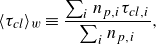
Following Liu et al. (Reference Liu, Shen, Zamansky and Coletti2020), we regard clusters in successive time steps as the same entity if they share the majority of their particles. This method mirrors the philosophical inquiry of the Ship of Theseus (see, e.g. Rea Reference Rea1995). For example, consider two clusters A and B in two successive time steps. The fraction of forward-in-time connection is defined as the number of particles shared by A and B divided by the total number of particles in A; while the fraction of backward-in-time connection is the number of shared particles divided by the total number of particles in B. Clusters A and B are considered continuous manifestations of the same cluster if their fraction of forward- and backward-in-time connections both exceed 0.5, and their lifetime is the time during which such a condition is continuously verified. We then estimate the weighted-averaged cluster lifetime $\langle \tau _{cl} \rangle _{w}$
as
$\langle \tau _{cl} \rangle _{w}$
as
 \begin{equation} \langle \tau _{cl} \rangle _{w} \equiv \frac {\sum _{i} n_{p,i} \tau _{cl,i}}{\sum _{i}n_{p,i}}, \end{equation}
where $\tau _{cl,i}$
is the lifetime of the
$\tau _{cl,i}$
is the lifetime of the $i$
th cluster.
$i$
th cluster.
To compare among different cases, the cluster lifetime is to be normalised by a time scale that reflects the particle–fluid dynamics. A natural choice is the eddy turnover time of the underlying flow, $L_F/u_{rms,f}$
. This is verified by analysing the dispersion and stretching of the group of particles that initially belong to a cluster. We use singular value decomposition (Baker et al. Reference Baker, Frankel, Mani and Coletti2017; Petersen, Baker & Coletti Reference Petersen, Baker and Coletti2019), which identifies the first principal axis along the main direction of spread, the second axis being orthogonal to it. The corresponding singular values,
$L_F/u_{rms,f}$
. This is verified by analysing the dispersion and stretching of the group of particles that initially belong to a cluster. We use singular value decomposition (Baker et al. Reference Baker, Frankel, Mani and Coletti2017; Petersen, Baker & Coletti Reference Petersen, Baker and Coletti2019), which identifies the first principal axis along the main direction of spread, the second axis being orthogonal to it. The corresponding singular values, $s_1$
and
$s_1$
and $s_2$
, are proportional to the spread of particle centroids along these axes. Figure 11(a) shows a representative example of temporal evolution of the normalised length scale
$s_2$
, are proportional to the spread of particle centroids along these axes. Figure 11(a) shows a representative example of temporal evolution of the normalised length scale $\langle R_g (t) / R_{g,0} \rangle$
and anisotropy
$\langle R_g (t) / R_{g,0} \rangle$
and anisotropy $[s_2 (t) / s_1 (t)]/[s_{2,0}/s_{1,0}]$
, where the subscript 0 indicates the time when the cluster is first identified. The trend confirms that sizeable changes to the spatial organisation occur within a time
$[s_2 (t) / s_1 (t)]/[s_{2,0}/s_{1,0}]$
, where the subscript 0 indicates the time when the cluster is first identified. The trend confirms that sizeable changes to the spatial organisation occur within a time $O(L_F / u_{rms,f})$
.
$O(L_F / u_{rms,f})$
.
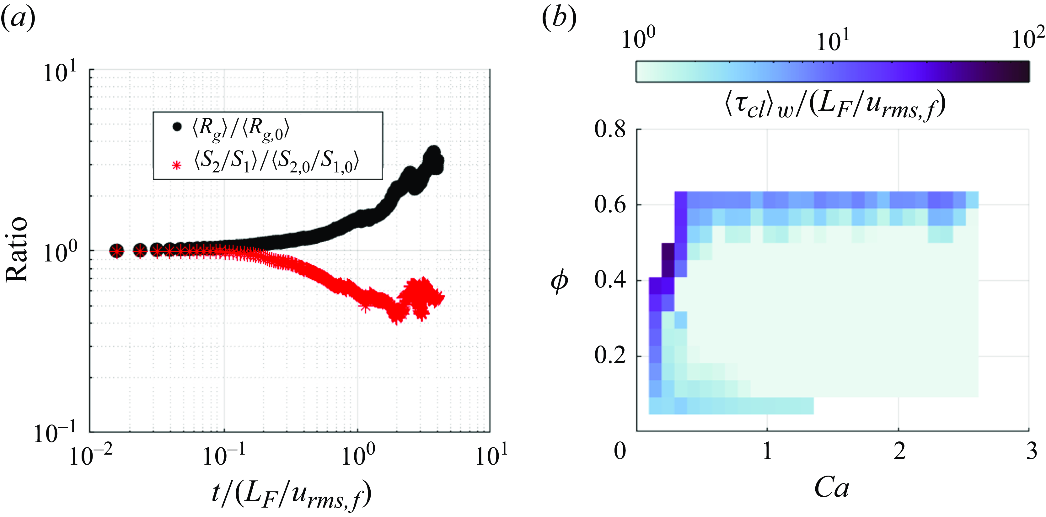
Figure 11. (a) Temporal evolution of the cluster size $\langle R_g(t)/R_{g,0} \rangle$
and cluster anisotropy
$\langle R_g(t)/R_{g,0} \rangle$
and cluster anisotropy $\langle [s_2(t)/s_1(t)]/[s_{2,0}/s_{1,0}] \rangle$
for an example case with
$\langle [s_2(t)/s_1(t)]/[s_{2,0}/s_{1,0}] \rangle$
for an example case with $Ca = 2.49$
and
$Ca = 2.49$
and $\phi = 0.44$
. (b) Contour map of the weighted average cluster lifetime
$\phi = 0.44$
. (b) Contour map of the weighted average cluster lifetime $\langle \tau _{{cl}} \rangle _w$
normalised by the flow turnover time
$\langle \tau _{{cl}} \rangle _w$
normalised by the flow turnover time $L_F/u_{{rms},f}$
across the
$L_F/u_{{rms},f}$
across the $Ca-\phi$
space.
$Ca-\phi$
space.
For a given eddy turnover time, however, the cluster lifetime can be significantly larger or smaller depending on the balance of the forces at play. Figure 11(b) displays a contour map of the normalised cluster lifetime in the $Ca-\phi$
space. As expected, clusters have longer lifetimes for lower
$Ca-\phi$
space. As expected, clusters have longer lifetimes for lower $Ca$
, where cohesive capillary forces dominate. As
$Ca$
, where cohesive capillary forces dominate. As $Ca$
increases, particularly in the moderately dense regime (
$Ca$
increases, particularly in the moderately dense regime ( $\phi \lt 0.4$
), clusters can live for just a fraction of the eddy turnover time before getting disrupted by the high strain rate of the intensely turbulent flow. On the other hand, in the denser regimes (
$\phi \lt 0.4$
), clusters can live for just a fraction of the eddy turnover time before getting disrupted by the high strain rate of the intensely turbulent flow. On the other hand, in the denser regimes ( $\phi \gt 0.4$
) the cluster lifetimes can far exceed
$\phi \gt 0.4$
) the cluster lifetimes can far exceed $L_F/u_{rms,f}$
irrespective of
$L_F/u_{rms,f}$
irrespective of $Ca$
. This is due to large clusters being brought about by excluded volume effects and kept together by lubrication. The particle dynamics within these large clusters, however, does vary substantially depending on
$Ca$
. This is due to large clusters being brought about by excluded volume effects and kept together by lubrication. The particle dynamics within these large clusters, however, does vary substantially depending on $Ca$
, as we show in the next section.
$Ca$
, as we show in the next section.
3.2. Particle dynamics
3.2.1. Single-particle dispersion
In Shin & Coletti (Reference Shin and Coletti2024), we demonstrated how Eulerian properties of the particle motion, in particular their fluctuating kinetic energy, vary within the $Ca-\phi$
space. Here we focus on Lagrangian transport, which we first characterise in terms of the single-particle dispersion. It is worth remarking that the peculiar properties of 2-D turbulent flows impact the Lagrangian dispersion. In particular, as shown by Xia et al. (Reference Xia, Francois, Punzmann and Shats2013) and confirmed by Shin et al. (Reference Shin, Coletti and Conlin2023), the length scale that determines the dispersion process is the forcing scale
$Ca-\phi$
space. Here we focus on Lagrangian transport, which we first characterise in terms of the single-particle dispersion. It is worth remarking that the peculiar properties of 2-D turbulent flows impact the Lagrangian dispersion. In particular, as shown by Xia et al. (Reference Xia, Francois, Punzmann and Shats2013) and confirmed by Shin et al. (Reference Shin, Coletti and Conlin2023), the length scale that determines the dispersion process is the forcing scale $L_F$
. This is at odds with the behaviour of 3-D turbulence, where dispersion is driven by the range of scales in which most energy reside. This characteristic was confirmed also in the transport of finite-size particles in Q2-D turbulence (Xia et al. Reference Xia, Francois, Punzmann and Shats2019).
$L_F$
. This is at odds with the behaviour of 3-D turbulence, where dispersion is driven by the range of scales in which most energy reside. This characteristic was confirmed also in the transport of finite-size particles in Q2-D turbulence (Xia et al. Reference Xia, Francois, Punzmann and Shats2019).
In the following, we consider the displacement $\boldsymbol{r}_i$
of the
$\boldsymbol{r}_i$
of the $i$
th particle from an initial position at time
$i$
th particle from an initial position at time $t_0$
, and calculate the mean squared displacement (MSD) by averaging over all particles and initial times
$t_0$
, and calculate the mean squared displacement (MSD) by averaging over all particles and initial times
 \begin{equation} \big\langle r^{2}(t) \big\rangle = \big\langle |\boldsymbol{x}_{i}(t_{0}+t) - \boldsymbol{x}_{i}(t_{0})|^{2} \big\rangle _{i,t_{0}}, \end{equation}
where $\boldsymbol{x}_i$
represents the centroid position of the
$\boldsymbol{x}_i$
represents the centroid position of the $i$
th particle. As the Lagrangian velocity autocorrelation
$i$
th particle. As the Lagrangian velocity autocorrelation $\Gamma _{L}(t) = \langle {\boldsymbol{u}_{i}(t_{0})\cdot \boldsymbol{u}_{i}(t_{0}+t)}\rangle _{i,t_{0}} / \langle {\boldsymbol{u}_{i}(t_{0})\cdot \boldsymbol{u}_{i}(t_{0})}\rangle _{i,t_{0}}$
approximates an exponential decay of characteristic time
$\Gamma _{L}(t) = \langle {\boldsymbol{u}_{i}(t_{0})\cdot \boldsymbol{u}_{i}(t_{0}+t)}\rangle _{i,t_{0}} / \langle {\boldsymbol{u}_{i}(t_{0})\cdot \boldsymbol{u}_{i}(t_{0})}\rangle _{i,t_{0}}$
approximates an exponential decay of characteristic time $t_L$
, one expects the classic scaling
$t_L$
, one expects the classic scaling $\langle r^{2}(t) \rangle \approx u_{rms}^{2} t^{2}$
for
$\langle r^{2}(t) \rangle \approx u_{rms}^{2} t^{2}$
for $t \ll t_L$
, and
$t \ll t_L$
, and $\langle r^{2}(t) \rangle \approx 2u_{rms}^{2} t_{L} t$
for
$\langle r^{2}(t) \rangle \approx 2u_{rms}^{2} t_{L} t$
for $t \gg t_L$
, where
$t \gg t_L$
, where $u_{rms}$
is the root-mean-squared velocity. The approximately exponential decay of
$u_{rms}$
is the root-mean-squared velocity. The approximately exponential decay of $\Gamma _L$
for the turbulent flow was demonstrated in Shin et al. (Reference Shin, Coletti and Conlin2023) over a Lagrangian time scale of the flow that we term
$\Gamma _L$
for the turbulent flow was demonstrated in Shin et al. (Reference Shin, Coletti and Conlin2023) over a Lagrangian time scale of the flow that we term $t_{L,f}$
. For the particles,
$t_{L,f}$
. For the particles, $\Gamma _L$
is shown by figure 12(a) in the example case
$\Gamma _L$
is shown by figure 12(a) in the example case $Ca = 0.87$
and
$Ca = 0.87$
and $\phi = 0.26$
. The characteristic time of the Lagrangian particle motion,
$\phi = 0.26$
. The characteristic time of the Lagrangian particle motion, $t_{L,p}$
, is taken as the e-fold decay time of
$t_{L,p}$
, is taken as the e-fold decay time of $\Gamma _L$
and found to be comparable to the turnover time of the particle motion,
$\Gamma _L$
and found to be comparable to the turnover time of the particle motion, $L_F/u_{rms,p}$
. Figure 12(b) plots the MSD for the particles, confirming the expected short-time and long-time behaviours with a ballistic-to-diffusive transition around
$L_F/u_{rms,p}$
. Figure 12(b) plots the MSD for the particles, confirming the expected short-time and long-time behaviours with a ballistic-to-diffusive transition around $t \sim t_{L,p}$
.
$t \sim t_{L,p}$
.
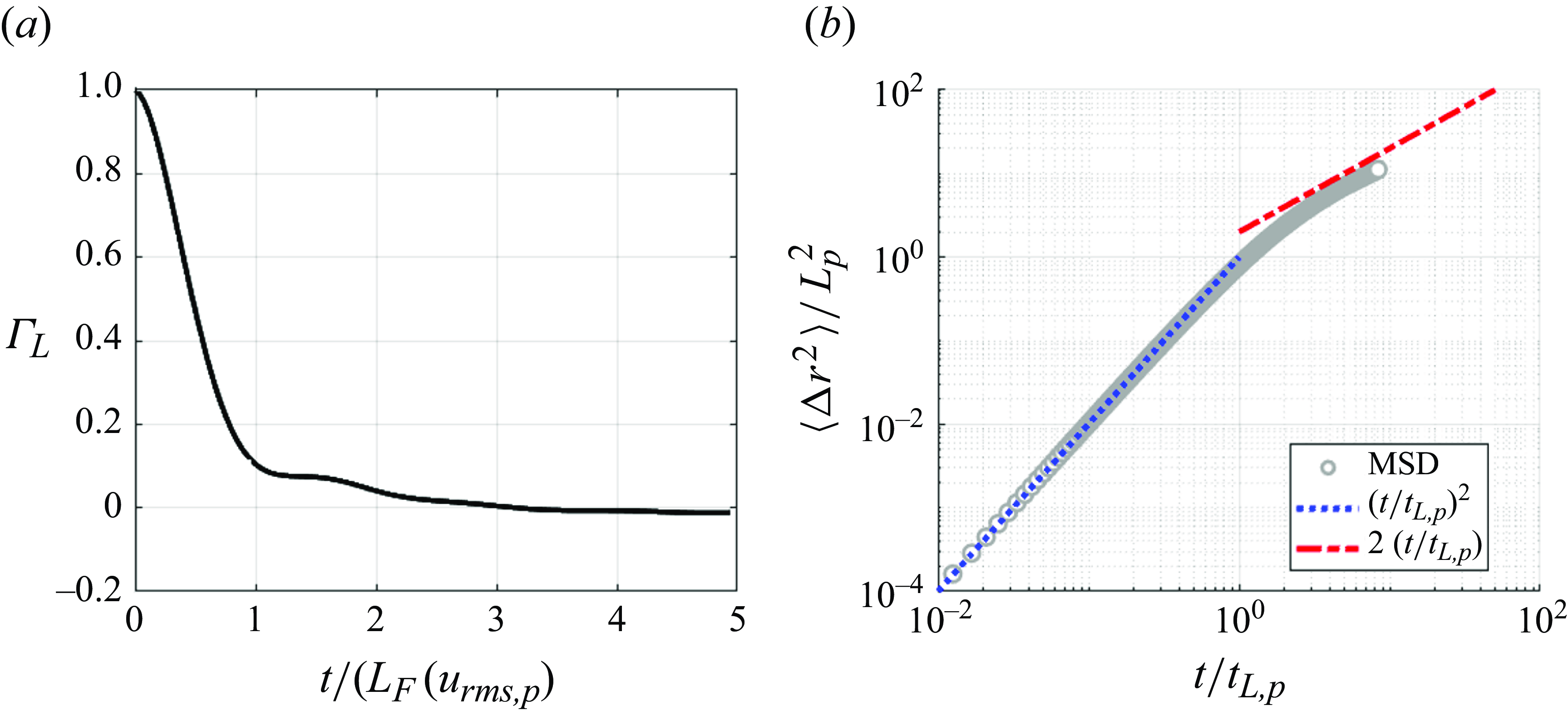
Figure 12. An example of (a) the Lagrangian velocity autocorrelation function (VACF) and (b) the MSD of particles for the case $Ca = 0.87$
and
$Ca = 0.87$
and $\phi = 0.27$
. The blue dotted line and red dash-dot line represent the short-term ballistic and long-term diffusive predictions, respectively, based on an exponentially decaying VACF with characteristic time scale
$\phi = 0.27$
. The blue dotted line and red dash-dot line represent the short-term ballistic and long-term diffusive predictions, respectively, based on an exponentially decaying VACF with characteristic time scale $t_{L,p}$
. The time is normalised by
$t_{L,p}$
. The time is normalised by $t_{L,p}$
, and the MSD is normalised by
$t_{L,p}$
, and the MSD is normalised by $L_p^{2} = (u_{rms,p} t_{L,p})^{2}$
.
$L_p^{2} = (u_{rms,p} t_{L,p})^{2}$
.
The diffusive behaviour allows us to evaluate the long-term diffusivity associated with the particle motion as (Taylor Reference Taylor1922; Davidson Reference Davidson2015)
 \begin{equation} K_p=\frac {1}{2} \frac {d \big\langle r^{2}(t) \big\rangle }{dt} \approx u_{rms,p} L_{p} = u_{rms,p}^{2} t_{L,p}, \end{equation}
where $L_p = u_{rms,p} t_{L,p}$
is a characteristic length scale of the particle motion. This is compared with the turbulent diffusivity of the fluid flow
$L_p = u_{rms,p} t_{L,p}$
is a characteristic length scale of the particle motion. This is compared with the turbulent diffusivity of the fluid flow $K_f$
, defining the normalised particle diffusivity
$K_f$
, defining the normalised particle diffusivity
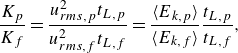 \begin{equation} \frac {K_p}{K_f} = \frac {u_{rms,p}^{2} t_{L,p}}{u_{rms,f}^{2} t_{L,f}} = \frac {\langle E_{k,p} \rangle }{\langle E_{k,f} \rangle } \frac {t_{L,p}}{t_{L,f}}, \end{equation}
where $\langle E_{k,p} \rangle$
and
$\langle E_{k,p} \rangle$
and $\langle E_{k,f} \rangle$
are the mean kinetic energies of particles and fluid, respectively. Figures 13(a) and 13(b) map in the
$\langle E_{k,f} \rangle$
are the mean kinetic energies of particles and fluid, respectively. Figures 13(a) and 13(b) map in the $Ca-\phi$
space the two factors: the particle-to-fluid ratio of fluctuating energy
$Ca-\phi$
space the two factors: the particle-to-fluid ratio of fluctuating energy $\langle E_{k,p} \rangle /\langle E_{k,f} \rangle$
, and the particle-to-fluid ratio of Lagrangian time scales
$\langle E_{k,p} \rangle /\langle E_{k,f} \rangle$
, and the particle-to-fluid ratio of Lagrangian time scales $t_{L,p}/t_{L,f}$
, respectively. Figure 13(a) reflects the observations made by Shin & Coletti (Reference Shin and Coletti2024). In the capillary-driven clustering regime (
$t_{L,p}/t_{L,f}$
, respectively. Figure 13(a) reflects the observations made by Shin & Coletti (Reference Shin and Coletti2024). In the capillary-driven clustering regime ( $Ca \lt 1$
) clusters can grow larger than the typical eddy size
$Ca \lt 1$
) clusters can grow larger than the typical eddy size $L_F$
, thus their motion is hindered as they filter out the energy of the smaller flow scales. In the drag-driven break-up regime (
$L_F$
, thus their motion is hindered as they filter out the energy of the smaller flow scales. In the drag-driven break-up regime ( $Ca \gt 1, \phi \lt 0.4$
), where the tendency to clustering is reduced, individual particles and small clusters have little inertia and thus possess a fluctuating energy comparable to the tracers. In the lubrication-driven clustering regime (
$Ca \gt 1, \phi \lt 0.4$
), where the tendency to clustering is reduced, individual particles and small clusters have little inertia and thus possess a fluctuating energy comparable to the tracers. In the lubrication-driven clustering regime ( $Ca \gt 1, \phi \gt 0.4$
), the particle kinetic energy is largely dissipated by the interaction with adjacent particles. Figure 13(b) shows how, if a particle belongs to a large compact cluster, it exhibits a long-time-correlated motion as it moves collectively with other members of the cluster. This results in
$Ca \gt 1, \phi \gt 0.4$
), the particle kinetic energy is largely dissipated by the interaction with adjacent particles. Figure 13(b) shows how, if a particle belongs to a large compact cluster, it exhibits a long-time-correlated motion as it moves collectively with other members of the cluster. This results in $t_{L,p}/t_{L,f}$
exceeding unity for dense concentrations, in particular in the lubrication-driven clustering regime. The particle diffusivity in figure 13(c) is the result of both competing trends: reduced energy and longer time correlation for large/compact clusters, and vice versa. Quantitatively, the trend of the fluctuating energy prevails, and the map of
$t_{L,p}/t_{L,f}$
exceeding unity for dense concentrations, in particular in the lubrication-driven clustering regime. The particle diffusivity in figure 13(c) is the result of both competing trends: reduced energy and longer time correlation for large/compact clusters, and vice versa. Quantitatively, the trend of the fluctuating energy prevails, and the map of $K_p/K_f$
in the
$K_p/K_f$
in the $Ca-\phi$
space closely resembles that of
$Ca-\phi$
space closely resembles that of $\langle E_{k,p} \rangle /\langle E_{k,f} \rangle$
. In conclusion, the clustering fostered by capillarity and lubrication reduces the particles’ ability to diffuse through the system.
$\langle E_{k,p} \rangle /\langle E_{k,f} \rangle$
. In conclusion, the clustering fostered by capillarity and lubrication reduces the particles’ ability to diffuse through the system.
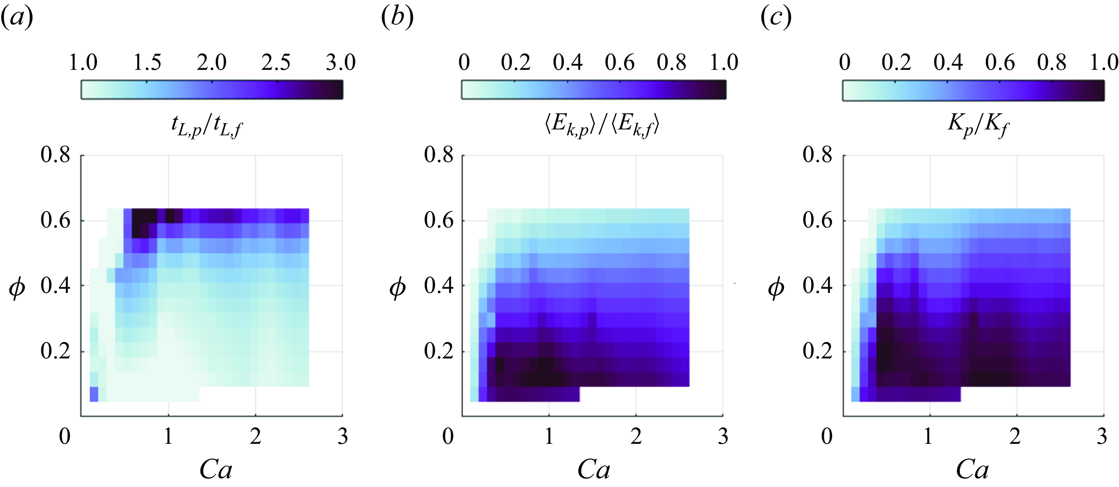
Figure 13. Contour maps in the $Ca-\phi$
space of (a) the ratio of Lagrangian time scales
$Ca-\phi$
space of (a) the ratio of Lagrangian time scales $t_{L,p} / t_{L,f}$
, (b) the ratio of particle to fluid kinetic energy
$t_{L,p} / t_{L,f}$
, (b) the ratio of particle to fluid kinetic energy $\langle E_{k,p} \rangle / \langle E_{k,f} \rangle$
and (c) the normalised particle turbulence diffusivity
$\langle E_{k,p} \rangle / \langle E_{k,f} \rangle$
and (c) the normalised particle turbulence diffusivity $K_p / K_f$
.
$K_p / K_f$
.
3.2.2. Velocity structure functions
Pair statistics are a classic tool to reveal how particles move relatively to each other. In order to highlight the dynamics of the aggregates, we restrict our attention to pairs of particles belonging to the same clusters, although this does not change the trend with respect to the unconditioned data analysis. We begin by considering the longitudinal and transverse second-order velocity structure functions, defined respectively as
 \begin{equation} S_2^L(r) = \left \langle \left ( \delta \boldsymbol{u}_{ij} \cdot \frac {\boldsymbol{r}_{ij}}{r} \right )^{2} \right \rangle , \end{equation}
 \begin{equation} S_2^T(r) = \left \langle \left ( \delta \boldsymbol{u}_{ij} - \delta \boldsymbol{u}_{ij} \cdot \frac {\boldsymbol{r_{ij}}}{r} \right )^{2} \right \rangle . \end{equation}
Here, $\delta \boldsymbol{u}_{ij} = \boldsymbol{u}_j - \boldsymbol{u}_i$
is the velocity difference between the
$\delta \boldsymbol{u}_{ij} = \boldsymbol{u}_j - \boldsymbol{u}_i$
is the velocity difference between the $i$
th and
$i$
th and $j$
th particles whose separation vector is
$j$
th particles whose separation vector is $\boldsymbol{r}_{ij} = \boldsymbol{x}_j - \boldsymbol{x}_i$
, with
$\boldsymbol{r}_{ij} = \boldsymbol{x}_j - \boldsymbol{x}_i$
, with $|\boldsymbol{r}_{ij}| = r$
. The longitudinal component corresponds to
$|\boldsymbol{r}_{ij}| = r$
. The longitudinal component corresponds to $\delta \boldsymbol{u}_{ij}$
projected along the direction of
$\delta \boldsymbol{u}_{ij}$
projected along the direction of $\boldsymbol{r}_{ij}$
, which is responsible for the particles’ separation, and the transverse component accounts for the element of
$\boldsymbol{r}_{ij}$
, which is responsible for the particles’ separation, and the transverse component accounts for the element of $\delta \boldsymbol{u}_{ij}$
perpendicular to
$\delta \boldsymbol{u}_{ij}$
perpendicular to $\boldsymbol{r}_{ij}$
, leading to rotation of the separation vector.
$\boldsymbol{r}_{ij}$
, leading to rotation of the separation vector.
Figures 14(a–c) compares structure functions for both particles and tracers for the same level of forcing, normalised by $u_{rms,p}^{2}$
and
$u_{rms,p}^{2}$
and $u_{rms,f}^{2}$
, respectively. The three identified regimes display distinctly different behaviours. In the capillary-driven clustering regime (figure 14
a), both
$u_{rms,f}^{2}$
, respectively. The three identified regimes display distinctly different behaviours. In the capillary-driven clustering regime (figure 14
a), both $S_2^L$
and
$S_2^L$
and $S_2^T$
are lower than those of tracers. Particles are tightly bound by capillarity within compact clusters, thus they translate collectively with relatively small longitudinal velocity differences. The transverse component of the relative velocity is inhibited to a degree that depends on the cluster size, but in general much less so than its longitudinal counterpart. In the drag-driven break-up regime (figure 14
b), clusters cannot be sustained in the region of high strain rate, thus they tend to reside in large vortex cores where they spin as quasi-rigid bodies. As those compact clusters spin, the particles in them that are separated by relatively large distances attain a rotational motion (with respect to each other) even faster than fluid parcels at equivalent separation. In those same clusters, on the other hand, inter-particle interactions limit the longitudinal separation rate. In the lubrication-driven clustering regime (figure 14
c), particle adjacency imposed by excluded volume leads to the formation of large clusters spanning multiple eddies. While their lifetime is relatively long (see § 3.1.4), they are continuously deformed by the underlying turbulent flow, and their normalised
$S_2^T$
are lower than those of tracers. Particles are tightly bound by capillarity within compact clusters, thus they translate collectively with relatively small longitudinal velocity differences. The transverse component of the relative velocity is inhibited to a degree that depends on the cluster size, but in general much less so than its longitudinal counterpart. In the drag-driven break-up regime (figure 14
b), clusters cannot be sustained in the region of high strain rate, thus they tend to reside in large vortex cores where they spin as quasi-rigid bodies. As those compact clusters spin, the particles in them that are separated by relatively large distances attain a rotational motion (with respect to each other) even faster than fluid parcels at equivalent separation. In those same clusters, on the other hand, inter-particle interactions limit the longitudinal separation rate. In the lubrication-driven clustering regime (figure 14
c), particle adjacency imposed by excluded volume leads to the formation of large clusters spanning multiple eddies. While their lifetime is relatively long (see § 3.1.4), they are continuously deformed by the underlying turbulent flow, and their normalised $S_2^L$
and
$S_2^L$
and $S_2^T$
approach those of tracers.
$S_2^T$
approach those of tracers.
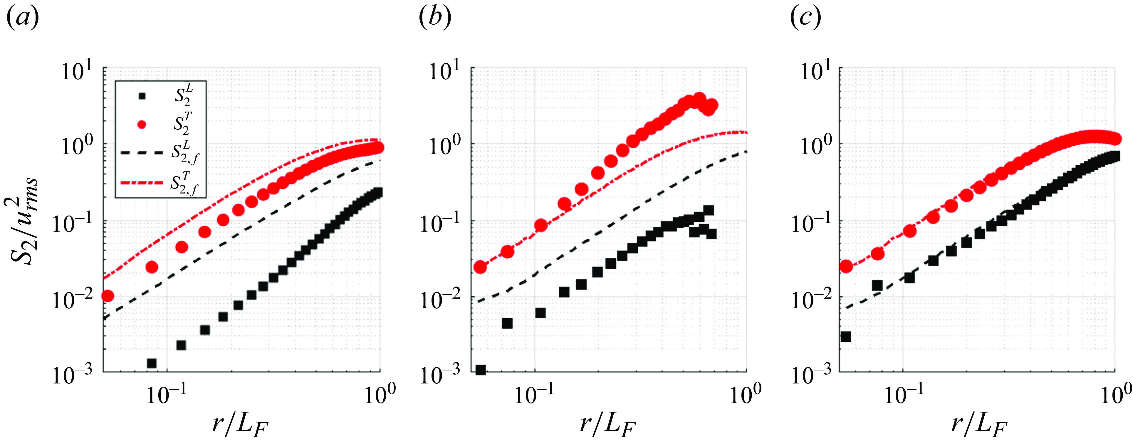
Figure 14. Examples of the second-order velocity structure functions ( $S_2$
) of particles from different experiments: (a)
$S_2$
) of particles from different experiments: (a) $Ca = 0.16$
and
$Ca = 0.16$
and $\phi = 0.14$
, (b)
$\phi = 0.14$
, (b) $Ca = 1.82$
and
$Ca = 1.82$
and $\phi = 0.27$
and (c)
$\phi = 0.27$
and (c) $Ca = 2.69$
and
$Ca = 2.69$
and $\phi = 0.62$
. In each panel,
$\phi = 0.62$
. In each panel, $S_2^L$
(black squares) and
$S_2^L$
(black squares) and $S_2^T$
(red circles) are normalised by
$S_2^T$
(red circles) are normalised by $u_{rms,p}^{2}$
. The dashed and dash-dot lines represent
$u_{rms,p}^{2}$
. The dashed and dash-dot lines represent $S_2^L$
and
$S_2^L$
and $S_2^T$
of tracers at the same level of forcing, respectively, normalised by
$S_2^T$
of tracers at the same level of forcing, respectively, normalised by $u_{rms,f}^{2}$
.
$u_{rms,f}^{2}$
.
3.2.3. Particle pair dispersion
Finally, we characterise the particle relative dispersion in a Lagrangian framework. To this end, we measure the mean squared separation (MSS) by tracking the evolution of the separation vector $\boldsymbol{r}_{ij}$
between particle pairs as a function of time
$\boldsymbol{r}_{ij}$
between particle pairs as a function of time
 \begin{equation} MSS(t) = \big\langle |\boldsymbol{r}_{ij}(t_0 + t) - \boldsymbol{r}_{ij}(t_0)|^{2} \big\rangle . \end{equation}
We focus on particle pairs that are initially adjacent, i.e. for which, at the initial time, $r_{ij,0} \sim {d}_p$
.
$r_{ij,0} \sim {d}_p$
.
To define the normalisation time scale, we first resort to the theory of 2-D turbulence. In the enstrophy cascade subrange, classical arguments for the separation law of particle pairs in smooth flows predict an exponential growth of the MSS at short times, with a characteristic time scale $t_{\zeta } = \zeta ^{-1/3}$
, where
$t_{\zeta } = \zeta ^{-1/3}$
, where $\zeta \equiv \nu \langle |\nabla \omega |^{2} \rangle$
is the enstrophy dissipation rate and
$\zeta \equiv \nu \langle |\nabla \omega |^{2} \rangle$
is the enstrophy dissipation rate and $\omega$
is the vorticity (Jullien Reference Jullien2003). We estimate
$\omega$
is the vorticity (Jullien Reference Jullien2003). We estimate $\zeta$
by modelling the flow field as an array of Taylor–Green vortices (Shin et al. Reference Shin, Coletti and Conlin2023)
$\zeta$
by modelling the flow field as an array of Taylor–Green vortices (Shin et al. Reference Shin, Coletti and Conlin2023)
 \begin{equation} \zeta /\nu = \big\langle |\nabla \omega |^{2} \big\rangle = \frac {4 \pi ^{4} u_{rms,f}^{2}}{L_{F}^{4}} .\end{equation}
This simplification yields quantitative agreement with the PIV measurements (figure 15 a).
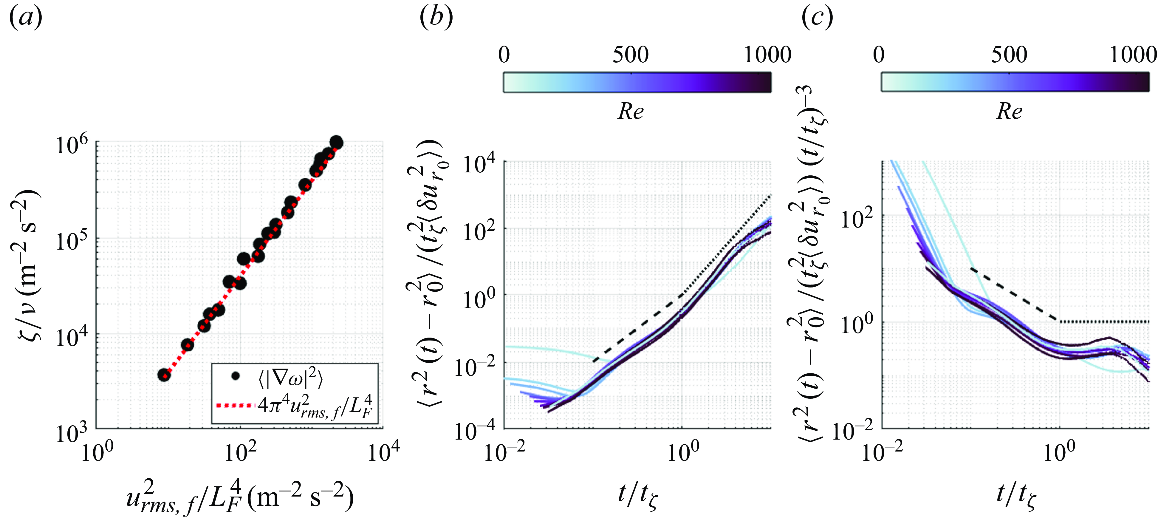
Figure 15. (a) Relationship between the enstrophy dissipation rate divided by the kinematic viscosity ( $\zeta / \nu$
) and
$\zeta / \nu$
) and $u_{rms,f}^{2} / L_F^{4}$
. Markers are obtained from PIV analysis of tracer experiments, and the red dotted line represents the estimation based on Taylor–Green vortices with a slope of
$u_{rms,f}^{2} / L_F^{4}$
. Markers are obtained from PIV analysis of tracer experiments, and the red dotted line represents the estimation based on Taylor–Green vortices with a slope of $4\pi ^{4}$
. (b) Examples of the MSS of tracers in the DL configuration at different levels of forcing, with an initial separation of 1.84 mm. The dashed and dash-dot lines indicate
$4\pi ^{4}$
. (b) Examples of the MSS of tracers in the DL configuration at different levels of forcing, with an initial separation of 1.84 mm. The dashed and dash-dot lines indicate $t^{2}$
and
$t^{2}$
and $t^3$
scalings, respectively. (c) Compensated MSS, where the MSS is divided by
$t^3$
scalings, respectively. (c) Compensated MSS, where the MSS is divided by $(t / t_\zeta )^3$
, highlighting the
$(t / t_\zeta )^3$
, highlighting the $t^3$
scaling as a plateau.
$t^3$
scaling as a plateau.
Based on this estimate, we approximate the characteristic time scale as $t_{\zeta } \approx (4 \pi ^{4} \nu u_{rms,f}^{2} / L_F^{4})^{-1/3}$
. For short times (
$t_{\zeta } \approx (4 \pi ^{4} \nu u_{rms,f}^{2} / L_F^{4})^{-1/3}$
. For short times ( $t \ll t_{\zeta }$
), the MSS is primarily influenced by the initial velocity difference,
$t \ll t_{\zeta }$
), the MSS is primarily influenced by the initial velocity difference, $\langle \delta u_{r}^{2}(t) \rangle \approx \langle \delta u_{r_{0}}^{2} \rangle$
. We therefore rescale the MSS as
$\langle \delta u_{r}^{2}(t) \rangle \approx \langle \delta u_{r_{0}}^{2} \rangle$
. We therefore rescale the MSS as $\langle |\boldsymbol{r}_{ij}(t_0 + t) - \boldsymbol{r}_{ij}(t_0)|^{2} \rangle /(t_{\zeta }^{2} \langle \delta u_{r_{0}}^{2} \rangle )$
, similar to Li et al. (Reference Li, Wang, Qi and Coletti2024) who studied pair-dispersion in free-surface turbulence, with
$\langle |\boldsymbol{r}_{ij}(t_0 + t) - \boldsymbol{r}_{ij}(t_0)|^{2} \rangle /(t_{\zeta }^{2} \langle \delta u_{r_{0}}^{2} \rangle )$
, similar to Li et al. (Reference Li, Wang, Qi and Coletti2024) who studied pair-dispersion in free-surface turbulence, with $t_{\zeta }$
replacing their transition time
$t_{\zeta }$
replacing their transition time $t_{D}$
between ballistic and diffusive behaviours of the relative velocity
$t_{D}$
between ballistic and diffusive behaviours of the relative velocity $\delta u$
.
$\delta u$
.
Figure 15(b) presents normalised MSS curves from tracers in the DL configuration, with an initial separation $r_{ij,0} \sim {d}_p$
. This is close to the range of initial separation of
$r_{ij,0} \sim {d}_p$
. This is close to the range of initial separation of $2-4\eta$
that Tan & Ni (Reference Tan and Ni2022) proposed as an upper limit for observing the super-diffusive scaling
$2-4\eta$
that Tan & Ni (Reference Tan and Ni2022) proposed as an upper limit for observing the super-diffusive scaling $\langle |\boldsymbol{r}_{ij}(t_0 + t) - \boldsymbol{r}_{ij}(t_0)|^{2} \rangle / \sim t^3$
in single-phase homogeneous turbulence. This scaling was originally proposed by Richardson (Reference Richardson1926) based on a scale-dependent diffusivity, and later justified by Obukhov (Reference Obukhov1941) as consistent with Kolmogorov’s (Reference Kolmogorov1941) theory. According to the latter, the dissipation rate of the turbulent kinetic energy is the only governing parameter in the inertial range, which dimensionally leads to the super-diffusive scaling. Here, the MSS curves collapse well on the chosen normalisation. For
$\langle |\boldsymbol{r}_{ij}(t_0 + t) - \boldsymbol{r}_{ij}(t_0)|^{2} \rangle / \sim t^3$
in single-phase homogeneous turbulence. This scaling was originally proposed by Richardson (Reference Richardson1926) based on a scale-dependent diffusivity, and later justified by Obukhov (Reference Obukhov1941) as consistent with Kolmogorov’s (Reference Kolmogorov1941) theory. According to the latter, the dissipation rate of the turbulent kinetic energy is the only governing parameter in the inertial range, which dimensionally leads to the super-diffusive scaling. Here, the MSS curves collapse well on the chosen normalisation. For $t/t_{\zeta } \ll 1$
, we note that experimental limitations such as resolution constraints affect the precise measurement of very small relative displacements of nearby tracers. This is likely the cause of the weak decline in separation observed at low Reynolds numbers. For
$t/t_{\zeta } \ll 1$
, we note that experimental limitations such as resolution constraints affect the precise measurement of very small relative displacements of nearby tracers. This is likely the cause of the weak decline in separation observed at low Reynolds numbers. For $t/t_{\zeta } \gt 1$
, the MSS curves display the super-diffusive scaling, and this persists until the separation grows beyond
$t/t_{\zeta } \gt 1$
, the MSS curves display the super-diffusive scaling, and this persists until the separation grows beyond $L_{F}$
, where the dispersion becomes purely diffusive.
$L_{F}$
, where the dispersion becomes purely diffusive.
The $t^3$
-scaling range (highlighted by the compensated plots in figure 15
c) is therefore limited by the scales of the system, and possibly by factors such as cross-scale contamination, which have made the super-diffusive regime particularly elusive (Bourgoin et al. Reference Bourgoin, Ouellette, Xu, Berg and Bodenschatz2006; Salazar & Collins Reference Salazar and Collins2009; Bitane, Homann & Bec Reference Bitane, Homann and Bec2012; Elsinga, Ishihara & Hunt Reference Elsinga, Ishihara and Hunt2022; Tan & Ni Reference Tan and Ni2022). The limited range over which the super-diffusive scaling is observed, and the fact that such an observation typically requires small initial separations (below the inertial range prescribed by Richardson–Obukhov theory) has created significant debate on the nature of the process in both 2-D and 3-D turbulence (Kellay & Goldburg Reference Kellay and Goldburg2002; Elsinga et al. Reference Elsinga, Ishihara and Hunt2022). This issue is, however, outside the scope of the present study: our interest is rather on how the particle dispersion compares with the fluid tracer dispersion, as we now discuss.
$t^3$
-scaling range (highlighted by the compensated plots in figure 15
c) is therefore limited by the scales of the system, and possibly by factors such as cross-scale contamination, which have made the super-diffusive regime particularly elusive (Bourgoin et al. Reference Bourgoin, Ouellette, Xu, Berg and Bodenschatz2006; Salazar & Collins Reference Salazar and Collins2009; Bitane, Homann & Bec Reference Bitane, Homann and Bec2012; Elsinga, Ishihara & Hunt Reference Elsinga, Ishihara and Hunt2022; Tan & Ni Reference Tan and Ni2022). The limited range over which the super-diffusive scaling is observed, and the fact that such an observation typically requires small initial separations (below the inertial range prescribed by Richardson–Obukhov theory) has created significant debate on the nature of the process in both 2-D and 3-D turbulence (Kellay & Goldburg Reference Kellay and Goldburg2002; Elsinga et al. Reference Elsinga, Ishihara and Hunt2022). This issue is, however, outside the scope of the present study: our interest is rather on how the particle dispersion compares with the fluid tracer dispersion, as we now discuss.
The observable width of the super-diffusive regime depends on the scale separation between the forcing scale $L_F$
and the initial separation. For separations much larger than
$L_F$
and the initial separation. For separations much larger than $L_F$
, the behaviour ultimately becomes diffusive, with a corresponding time scale roughly given by
$L_F$
, the behaviour ultimately becomes diffusive, with a corresponding time scale roughly given by $t_{L,p} \sim L_F/u_{rms,p}$
. In our analysis, the temporal scale separation between the inertial (ballistic or super-diffusive) regime and the diffusive regime scales approximately as
$t_{L,p} \sim L_F/u_{rms,p}$
. In our analysis, the temporal scale separation between the inertial (ballistic or super-diffusive) regime and the diffusive regime scales approximately as $t_{L,p}/t_{\zeta } \sim L_{F}^{-1/3}$
, modulated by the velocity ratio
$t_{L,p}/t_{\zeta } \sim L_{F}^{-1/3}$
, modulated by the velocity ratio $u_{rms,f}/u_{rms,p}$
at the given flow
$u_{rms,f}/u_{rms,p}$
at the given flow $Re$
. Thus, increasing
$Re$
. Thus, increasing $L_F$
would, in a purely temporal sense, slightly reduce the window over which super-diffusion is observed. Conversely, from a spatial perspective, it is crucial that
$L_F$
would, in a purely temporal sense, slightly reduce the window over which super-diffusion is observed. Conversely, from a spatial perspective, it is crucial that $L_F$
is significantly larger than the typical initial separation (which is lower bounded by the particle diameter
$L_F$
is significantly larger than the typical initial separation (which is lower bounded by the particle diameter ${d}_p$
); indeed, our results indicate that, if the initial separation exceeds approximately
${d}_p$
); indeed, our results indicate that, if the initial separation exceeds approximately $0.25L_F$
, the
$0.25L_F$
, the $t^3$
-scaling is not apparent and replaced by ballistic scaling (
$t^3$
-scaling is not apparent and replaced by ballistic scaling ( $\sim t^{2}$
). Moreover, when the particle velocity
$\sim t^{2}$
). Moreover, when the particle velocity $u_{rms,p}$
is much lower than the fluid velocity
$u_{rms,p}$
is much lower than the fluid velocity $u_{rms,f}$
– as observed at high areal fractions – the effective temporal separation is enhanced, thereby extending the super-diffusive regime.
$u_{rms,f}$
– as observed at high areal fractions – the effective temporal separation is enhanced, thereby extending the super-diffusive regime.
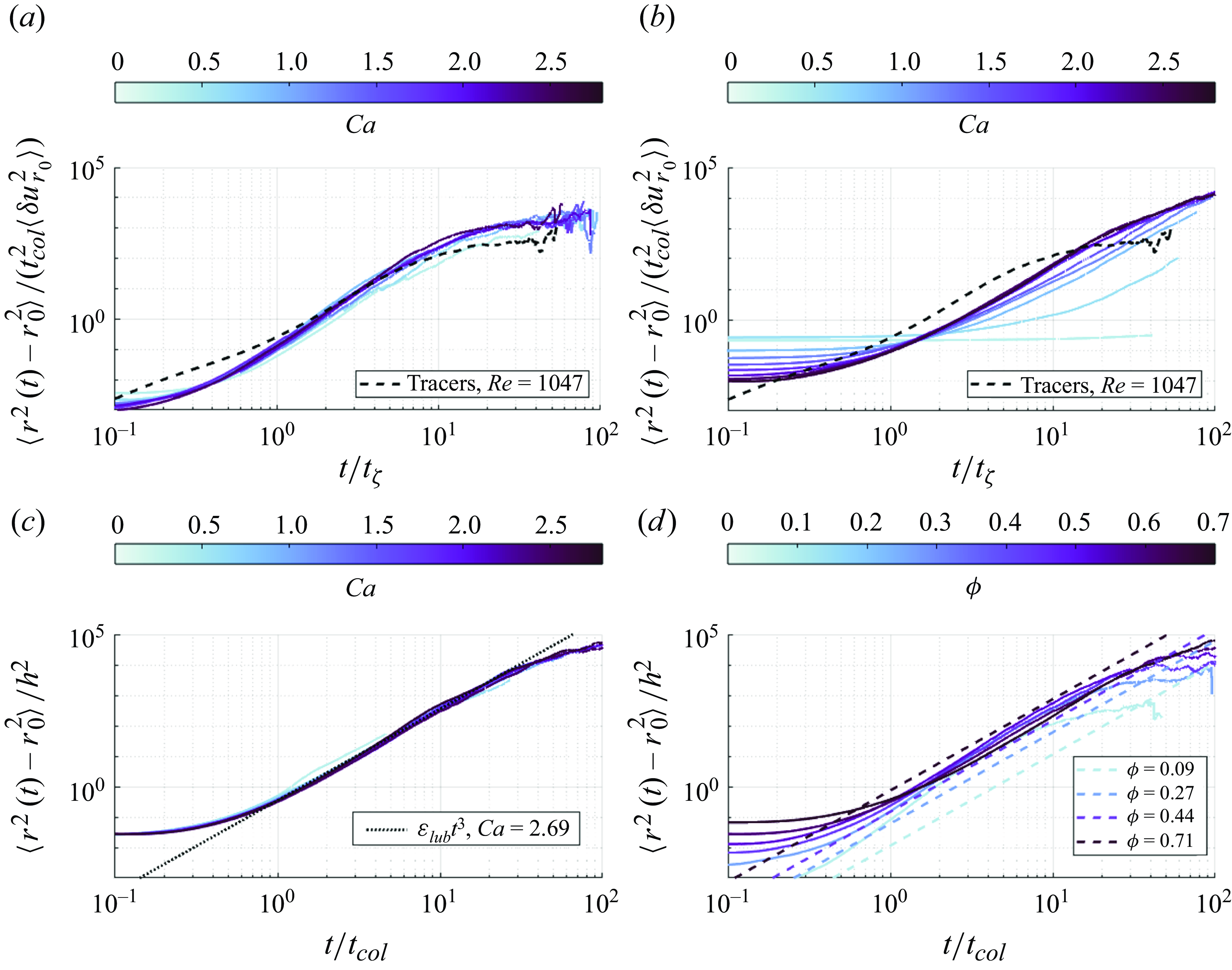
Figure 16. Examples of the MSS of particle pairs with an initial separation of ${d}_p = 1.84$
mm: (a)
${d}_p = 1.84$
mm: (a) $\phi = 0.27$
, and (b)
$\phi = 0.27$
, and (b) $\phi = 0.71$
. The dashed line corresponds to the MSS of tracers from the most turbulent flow in the experiments. (c) The MSS curves for high
$\phi = 0.71$
. The dashed line corresponds to the MSS of tracers from the most turbulent flow in the experiments. (c) The MSS curves for high $\phi = 0.62$
across varying
$\phi = 0.62$
across varying $Ca$
values, with time normalised by the collision time scale
$Ca$
values, with time normalised by the collision time scale $t_{col} = h / u_{rel}$
and MSS by
$t_{col} = h / u_{rel}$
and MSS by $h^{2}$
. The dotted line indicates the MSS prediction by (3.12). (d) The MSS curves at
$h^{2}$
. The dotted line indicates the MSS prediction by (3.12). (d) The MSS curves at $Ca = 2.49$
across different areal fractions, with lines indicating the MSS predictions by (3.12) at
$Ca = 2.49$
across different areal fractions, with lines indicating the MSS predictions by (3.12) at $\phi = 0.09$
, 0.27, 0.44 and 0.71 (dash-dot), respectively.
$\phi = 0.09$
, 0.27, 0.44 and 0.71 (dash-dot), respectively.
The relative dispersion of the particles is illustrated in figure 16 for different values of $Ca$
and
$Ca$
and $\phi$
, again for
$\phi$
, again for $r_0 \sim {d}_p$
. A dashed line showing the MSS of tracers for a representative case (weakly dependent on the forcing, as shown in figure 15) is included for reference. In the moderately dense case (
$r_0 \sim {d}_p$
. A dashed line showing the MSS of tracers for a representative case (weakly dependent on the forcing, as shown in figure 15) is included for reference. In the moderately dense case ( $\phi =0.27$
, figure 16
a), we observe slower initial dispersion at
$\phi =0.27$
, figure 16
a), we observe slower initial dispersion at $t/t_{\zeta } \lt 1$
, due to capillarity and lubrication inhibiting separation at small distances. Once particle pairs grow far enough apart that cohesive interactions become negligible, the curves at different
$t/t_{\zeta } \lt 1$
, due to capillarity and lubrication inhibiting separation at small distances. Once particle pairs grow far enough apart that cohesive interactions become negligible, the curves at different $Ca$
collapse and exhibit a super-diffusive scaling for over a decade, until the separation grows beyond
$Ca$
collapse and exhibit a super-diffusive scaling for over a decade, until the separation grows beyond $L_F$
.
$L_F$
.
At $\phi = 0.71$
(figure 16
b), the effect of
$\phi = 0.71$
(figure 16
b), the effect of $Ca$
becomes more prominent. At
$Ca$
becomes more prominent. At $Ca \ll 1$
, as the particle velocity is significantly slower than the fluid velocity (see figure 12
a), it takes much longer than
$Ca \ll 1$
, as the particle velocity is significantly slower than the fluid velocity (see figure 12
a), it takes much longer than $t_{\zeta }$
for a pair to separate enough to break away from their mutual attraction. Conversely, at
$t_{\zeta }$
for a pair to separate enough to break away from their mutual attraction. Conversely, at $Ca \gt 1$
particle separation occurs more rapidly and the super-diffusive regime is retrieved. This scaling of relative dispersion in such densely packed cases is striking, as most particles remain contained within a massively large, percolating cluster. This highlights the dynamic nature of clusters formed at high
$Ca \gt 1$
particle separation occurs more rapidly and the super-diffusive regime is retrieved. This scaling of relative dispersion in such densely packed cases is striking, as most particles remain contained within a massively large, percolating cluster. This highlights the dynamic nature of clusters formed at high $Ca$
, in contrast to the quasi-rigid clusters formed at low
$Ca$
, in contrast to the quasi-rigid clusters formed at low $Ca$
. This change in behaviour is not captured by the analysis of cluster lifetime, which shows no noticeable trend with
$Ca$
. This change in behaviour is not captured by the analysis of cluster lifetime, which shows no noticeable trend with $Ca$
at
$Ca$
at $\phi = 0.71$
(see figure 11
b).
$\phi = 0.71$
(see figure 11
b).
When using $t_{\zeta }$
for normalisation, the transition to the super-diffusive regime at dense concentrations occurs at different times. This is not surprising, as the fluid enstrophy is unlikely to be the governing factor at such high particle concentrations. We hypothesise that, for dense suspensions at high
$t_{\zeta }$
for normalisation, the transition to the super-diffusive regime at dense concentrations occurs at different times. This is not surprising, as the fluid enstrophy is unlikely to be the governing factor at such high particle concentrations. We hypothesise that, for dense suspensions at high $Ca$
(i.e. in the lubrication-driven clustering regime), the frequent inter-particle interactions via lubrication, rather than the fluid enstrophy, become the dominant mechanism governing the energy dissipation and in turn the relative dispersion. For each particle, the energy dissipation rate due to lubrication is
$Ca$
(i.e. in the lubrication-driven clustering regime), the frequent inter-particle interactions via lubrication, rather than the fluid enstrophy, become the dominant mechanism governing the energy dissipation and in turn the relative dispersion. For each particle, the energy dissipation rate due to lubrication is $\varepsilon _{lub} \sim F_{lub} u_{rel}$
, where
$\varepsilon _{lub} \sim F_{lub} u_{rel}$
, where $F_{lub}$
is the lubrication force experienced by a particle moving with a velocity
$F_{lub}$
is the lubrication force experienced by a particle moving with a velocity $u_{rel}$
relative to its neighbour. Considering the particle number density per area
$u_{rel}$
relative to its neighbour. Considering the particle number density per area $n = 4\phi /(\pi {d}_p^{2})$
and the area density
$n = 4\phi /(\pi {d}_p^{2})$
and the area density $\rho _A = \rho _f \delta$
, where
$\rho _A = \rho _f \delta$
, where $\delta$
is the fluid layer thickness, the relevant short-range energy dissipation rate per unit mass can be approximated as
$\delta$
is the fluid layer thickness, the relevant short-range energy dissipation rate per unit mass can be approximated as
 \begin{equation} \varepsilon _{lub} \approx F_{lub} u_{rel} \frac {n}{\rho _A} \approx \frac {3\pi \mu {d}_p^{2} u_{rel}^{2} }{2h} \frac {4\phi /(\pi {d}_p^{2}) }{\rho _f \delta } = \frac {6 \nu _f u_{rel}^{2}}{\delta {d}_p} \frac {\phi }{[(\phi _{max}/\phi )^{0.5} - 1]}, \end{equation}
where $h = {d}_p[(\phi _{max}/\phi )^{0.5}-1]$
is the mean surface-to-surface separation between neighbouring particles, with
$h = {d}_p[(\phi _{max}/\phi )^{0.5}-1]$
is the mean surface-to-surface separation between neighbouring particles, with $\phi _{max} \approx 0.9064$
being the maximum areal fraction from the 2-D hexagonal close packing.
$\phi _{max} \approx 0.9064$
being the maximum areal fraction from the 2-D hexagonal close packing.
Under the assumption that $\varepsilon _{lub}$
is the main governing parameter, dimensional arguments yield immediately
$\varepsilon _{lub}$
is the main governing parameter, dimensional arguments yield immediately $MSS \sim \varepsilon _{lub} t^3$
, and therefore
$MSS \sim \varepsilon _{lub} t^3$
, and therefore
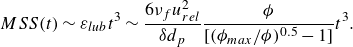 \begin{equation} MSS(t) \sim \varepsilon _{lub} t^3 \sim \frac{6\nu _f u_{rel}^2}{\delta {d}_p} \frac {\phi }{[(\phi _{max}/\phi )^{0.5} - 1]}t^{3} .\end{equation}
Here, the relevant length and time scale are associated with inter-particle collisions (meant in a general sense as direct interaction/contact), which we take as $h$
and
$h$
and $t_{col} = h/u_{rel}$
, respectively. Since the longitudinal second-order structure function
$t_{col} = h/u_{rel}$
, respectively. Since the longitudinal second-order structure function $S_{2,p}^L/u_{rms,p}^{2}$
of particles in the lubrication-driven clustering regime shows excellent quantitative agreement with
$S_{2,p}^L/u_{rms,p}^{2}$
of particles in the lubrication-driven clustering regime shows excellent quantitative agreement with $S_{2,f}^L/u_{rms,f}^{2}$
of tracers (figure 14
c), we approximate
$S_{2,f}^L/u_{rms,f}^{2}$
of tracers (figure 14
c), we approximate $u_{rel}(r) \sim u_{rms,p} (S_{2,f}^L(r)/u_{rms,f}^{2})^{0.5}$
, evaluated at
$u_{rel}(r) \sim u_{rms,p} (S_{2,f}^L(r)/u_{rms,f}^{2})^{0.5}$
, evaluated at $r=h$
. These length and time scales correspond to the distance and time over which a particle in a pair travels to encounter another neighbour whose centre is
$r=h$
. These length and time scales correspond to the distance and time over which a particle in a pair travels to encounter another neighbour whose centre is $h+{d}_p$
away from its own. For
$h+{d}_p$
away from its own. For $\phi \gt 0.4$
, the particles in densely packed suspensions are expected to forget their initial relative velocity through mutual interactions, with lubrication governing the decorrelation of their relative velocity.
$\phi \gt 0.4$
, the particles in densely packed suspensions are expected to forget their initial relative velocity through mutual interactions, with lubrication governing the decorrelation of their relative velocity.
This expectation is confirmed in figure 16(c,d), which plots the MSS curves for $\phi =0.62$
with varying
$\phi =0.62$
with varying $Ca$
values, and for
$Ca$
values, and for $Ca=2.49$
with varying
$Ca=2.49$
with varying $\phi$
values, respectively, normalised by
$\phi$
values, respectively, normalised by $t_{col}$
and
$t_{col}$
and $h^{2}$
. Figure 16(c) shows that this normalisation produces a tight collapse of the curves, which display a super-diffusive regime for
$h^{2}$
. Figure 16(c) shows that this normalisation produces a tight collapse of the curves, which display a super-diffusive regime for $t \gt t_{col}$
. Moreover, the super-diffusive MSS estimated for the highest
$t \gt t_{col}$
. Moreover, the super-diffusive MSS estimated for the highest $Ca$
using (3.12), based on the assumption that lubrication is the dominant energy dissipation mechanism in dense cases (indicated with a dotted line), shows good agreement with the experimental curve. We stress that such a scaling argument is expected to apply within a pre-factor of order unity. The agreement between (3.12) and the experimental MSS implies that
$Ca$
using (3.12), based on the assumption that lubrication is the dominant energy dissipation mechanism in dense cases (indicated with a dotted line), shows good agreement with the experimental curve. We stress that such a scaling argument is expected to apply within a pre-factor of order unity. The agreement between (3.12) and the experimental MSS implies that $\varepsilon _{lub}$
takes on the role of the turbulent dissipation rate in single-phase flows.
$\varepsilon _{lub}$
takes on the role of the turbulent dissipation rate in single-phase flows.
To further inspect the role of short-range interactions in MSS across different concentrations, we plot the normalised MSS curves at $Ca = 2.49$
across varying
$Ca = 2.49$
across varying $\phi$
values in figure 16(d). Dashed lines calculated using (3.12) indicate how the agreement progressively improves for increasing concentrations, as one transitions from the drag-driven break-up to the lubrication-driven clustering regime.
$\phi$
values in figure 16(d). Dashed lines calculated using (3.12) indicate how the agreement progressively improves for increasing concentrations, as one transitions from the drag-driven break-up to the lubrication-driven clustering regime.
4. Conclusion
We have investigated the mechanisms governing particle clustering and dispersion in dense turbulent interfacial suspensions of non-Brownian, monodisperse spherical particles at immiscible fluid interfaces. Building upon the phase diagram in the capillary number ( $Ca$
) and areal fraction (
$Ca$
) and areal fraction ( $\phi$
) space constructed in our previous work (Shin & Coletti Reference Shin and Coletti2024), we have provided a comprehensive analysis of cluster properties and the particle dynamics across different regimes. By systematically varying the capillary number
$\phi$
) space constructed in our previous work (Shin & Coletti Reference Shin and Coletti2024), we have provided a comprehensive analysis of cluster properties and the particle dynamics across different regimes. By systematically varying the capillary number $Ca$
and the areal fraction
$Ca$
and the areal fraction $\phi$
and analysing Lagrangian trajectories, we have characterised the clustering process via clustering fraction, cluster size distributions, percolation, fractal dimensions, hexatic order parameters and cluster lifetime. Additionally, we have explored the particle dynamics by examining single-particle dispersion, velocity structure functions and pair dispersion. Our findings reveal how the interplay between capillary forces, viscous drag and lubrication interactions dictates the behaviour of particles in these suspensions, leading to a distinct dynamics in different regions of the
$\phi$
and analysing Lagrangian trajectories, we have characterised the clustering process via clustering fraction, cluster size distributions, percolation, fractal dimensions, hexatic order parameters and cluster lifetime. Additionally, we have explored the particle dynamics by examining single-particle dispersion, velocity structure functions and pair dispersion. Our findings reveal how the interplay between capillary forces, viscous drag and lubrication interactions dictates the behaviour of particles in these suspensions, leading to a distinct dynamics in different regions of the $Ca-\phi$
phase space. Specifically, concerning clustering:
$Ca-\phi$
phase space. Specifically, concerning clustering:
-
(i) In the capillary-driven clustering regime ( $Ca\lt 1$
), capillary attractions dominate over viscous drag, leading to the formation of large clusters through hit-and-stick type collisions. These clusters can grow to sizes even larger than the typical eddy size and exhibit relatively low fractal dimensions. That is, they have a fractal-like structure akin to what observed in diffusion-limited processes, resulting from particles aggregating via capillary forces without significant rearrangement.
$Ca\lt 1$
), capillary attractions dominate over viscous drag, leading to the formation of large clusters through hit-and-stick type collisions. These clusters can grow to sizes even larger than the typical eddy size and exhibit relatively low fractal dimensions. That is, they have a fractal-like structure akin to what observed in diffusion-limited processes, resulting from particles aggregating via capillary forces without significant rearrangement. -
(ii) In the drag-driven break-up regime (
$Ca\gt 1, \phi \lt 0.40$
), increased turbulent fluctuations enhances viscous drag on the particles, which overcome capillary attraction. Particles tend to remain isolated or form small, short-lived clusters. The statistical properties of the clusters closely resemble those of random configurations generated by RSA processes: the clustering fraction, cluster size distributions and fractal dimensions approach those expected in random, non-interacting particle arrangements, indicating that clustering arises primarily due to random proximity rather than cohesive forces. -
(iii) In the lubrication-driven clustering regime (
$Ca\gt 1$
,
$\phi \gt 0.40$
), frequent inter-particle interactions due to high particle concentration amplify the role of lubrication forces. Despite strong turbulent forcing, particles can form large, dynamically evolving clusters that can span the entire system and live much longer than the energetic eddies. Lubrication forces hinder particle separation, leading to densely packed, crystal-like structures.


Above a threshold level of concentration that depends on $Ca$
, dense interfacial suspensions exhibit a percolation behaviour similar to what is observed in other non-turbulent particle systems. In particular, for
$Ca$
, dense interfacial suspensions exhibit a percolation behaviour similar to what is observed in other non-turbulent particle systems. In particular, for $Ca \lt 1$
the cluster size distribution follows a self-similar shape found in randomly generated aggregates; while for
$Ca \lt 1$
the cluster size distribution follows a self-similar shape found in randomly generated aggregates; while for $Ca \gt 1$
the behaviour resembles what predicted in coagulating agglomerates with equally probable interactions among all particles.
$Ca \gt 1$
the behaviour resembles what predicted in coagulating agglomerates with equally probable interactions among all particles.
As for the particle dispersion, single-particle analysis shows that clustering reduces the diffusivity by lowering their kinetic energy significantly, despite an extended time correlation of the motion. The velocity structure functions indicate that particles in the capillary-driven clustering regime have a limited relative velocity due to the strength of the bonds. This is the case also in the drag-driven break-up regime, in which clusters are mostly found in vortex cores and are spun as quasi-rigid bodies. In the lubrication-driven clustering regime, the large long-lived clusters are deformed by the turbulent flow and the particle relative velocities behave similarly to those of tracers, although with a reduced magnitude.
Analysis of the relative dispersion shows how, in the capillary-driven clustering regime, adjacent particle pairs separate at initially slow rates due to strong capillary attraction. Once this is overcome by turbulent fluctuations, the dispersion becomes super-diffusive until the separation exceeds the large-eddy size. In the drag-driven break-up regime, pair dispersion closely resembles that of passive tracers in turbulence. In the lubrication-driven clustering regime, due to the frequent particle–particle interactions at high concentrations, the collision rate defines the relevant time scale. This results in a regime where, after breaking away from each other, initially adjacent particles separate super-diffusively, but proportionally to the energy dissipation rate of the lubrication forces. Therefore, even though in this regime the clusters appear densely packed, their internal structure at intermediate scales is continuously rearranging.
The present work is limited to Q2-D settings with specific particle types and sizes. Factors like particle shape, size polydispersity and varying interfacial properties (such as the presence of surfactants) could affect the nature of the capillary attraction. The moderate $Re$
achieved may not capture all of the relevant dynamics present in more turbulent environments where the assumption of Stokesian dynamics could break down. Moreover, free-surface turbulent flows with sizeable depth are characterised by a compressible surface-velocity field which influences clustering and dispersion (Lovecchio, Marchioli & Soldati Reference Lovecchio, Marchioli and Soldati2013; Li et al. Reference Li, Wang, Qi and Coletti2024; Qi, Li & Coletti Reference Qi, Li and Coletti2025). Future research is warranted to address these limitations by exploring a broader range of particle characteristics, interfacial conditions and flow regimes to test the generality of our findings. The combination of drag, capillarity and lubrication that we use to rationalise the present system is indeed a simplification which does not take into account higher-order effects. For example, recent studies have demonstrated the existence of fluctuation-induced hydrodynamic forces acting on single or multiple objects (Yang et al. Reference Yang, Davoodianidalik, Xia, Punzmann, Shats and Francois2019; Spandan et al. Reference Spandan, Putt, Ostilla-Mónico and Lee2020; Davoodianidalik et al. Reference Davoodianidalik, Punzmann, Kellay, Xia, Shats and Francois2022). While explicitly quantifying such forces is beyond the scope of the present work, future studies shall investigate their role directly.
$Re$
achieved may not capture all of the relevant dynamics present in more turbulent environments where the assumption of Stokesian dynamics could break down. Moreover, free-surface turbulent flows with sizeable depth are characterised by a compressible surface-velocity field which influences clustering and dispersion (Lovecchio, Marchioli & Soldati Reference Lovecchio, Marchioli and Soldati2013; Li et al. Reference Li, Wang, Qi and Coletti2024; Qi, Li & Coletti Reference Qi, Li and Coletti2025). Future research is warranted to address these limitations by exploring a broader range of particle characteristics, interfacial conditions and flow regimes to test the generality of our findings. The combination of drag, capillarity and lubrication that we use to rationalise the present system is indeed a simplification which does not take into account higher-order effects. For example, recent studies have demonstrated the existence of fluctuation-induced hydrodynamic forces acting on single or multiple objects (Yang et al. Reference Yang, Davoodianidalik, Xia, Punzmann, Shats and Francois2019; Spandan et al. Reference Spandan, Putt, Ostilla-Mónico and Lee2020; Davoodianidalik et al. Reference Davoodianidalik, Punzmann, Kellay, Xia, Shats and Francois2022). While explicitly quantifying such forces is beyond the scope of the present work, future studies shall investigate their role directly.
Finally, the connections made with diffusion-limited aggregation, percolation theory and random particle systems emphasise potentially powerful links with research areas seldom intertwined with particle-laden fluid dynamics. For example, the present finding may be compared with the behaviour exhibited by active particles or colloids (Alert, Casademunt & Joanny Reference Alert, Casademunt and Joanny2022). These are driven by self-propulsion and thermal fluctuations, respectively, rather than turbulence in the carrier fluid. This results in qualitatively different behaviours, particularly concerning the inter-scale energy transfer. At high concentrations, on the other hand, the particle–particle interaction may prevail and similarities with the present class of dense turbulent suspensions might be expected. Any such analogy, however, is to be investigated by dedicated studies.
Funding
This work was supported by the Swiss National Science Foundation, grant number 200021-207318.
Declaration of interests
The authors report no conflict of interest.


 Open access