1. Introduce

Cable-driven parallel robots (CDPRs), as the name implies, are special robots that use flexible cables to connect a platform or gripper to a base, replacing traditional rigid arms. Because cables replace rigid rods, CDPRs have less inertia and a higher load ratio than traditional robots, which means they can achieve higher accelerations and speeds [Reference Zarebidoki, Dhupia and Xu1]. Currently, there are various types of CDPR structures, including classic CDPR with a fixed base [Reference Wang and Li2–Reference Li, Kui, Yao and Wu7], mobile CDPR with an unmanned vehicle as the base [Reference Liu, Cao, Xiong, Du, Cao and Zhang8], mobile CDPR with drones as the base [Reference Jiang and Kumar9, Reference Krizmancic, Arbanas, Petrovic, Petric and Bogdan10], and some CDPRs for special scenarios [Reference Zhang, Li, Wang, Shang, Gao, Ma, Yao, Li, Yin, Yang and Li11–Reference Sun, Tang, Cui and Hou14]. The most notable example is the cable-driven structure of the Five-Hundred-Meter Aperture Spherical Radio Telescope (FAST) in southwestern China, which is used to move the telescope’s feed module [Reference Zhang, Li, Wang, Shang, Gao, Ma, Yao, Li, Yin, Yang and Li11].

Although CDPRs have many advantages, their modeling difficulty is much higher than that of traditional rigid robots due to the use of flexible ropes. It not only includes the flexible nonlinearity and multi-variable coupling of the parallel robot, but it also includes the uncertainty and nonlinearity caused by the sag and stretching of the ropes [Reference Khan, Mohammadi, Rasmussen, Bai and Struijk15]. In order to establish a more accurate model, researchers have also conducted in-depth research on nonlinear friction models [Reference Ji, Shang and Cong6], error transmission models [Reference Gao, Zhou, Zi, Qian and Zhao5], error compensation [Reference Zhang, Shang, Li and Cong16], and measurement confusion identification [Reference Wang, Gao, Kinugawa and Kosuge17].

Even if the theoretical model is perfect, inaccurate model parameters caused by installation errors, rope deformation, etc. will still lead to a poor control effect of CDPR. Most literature often assumes that the rope length remains unchanged, ignores the adverse effects of parameter changes, and seeks to use control algorithms with good robustness to suppress the impact of model uncertainty. Li et al. [Reference Li, Kui, Yao and Wu7] proposed an adaptive integral sliding mode collaborative control algorithm, which effectively improved the robustness of the system. Lu et al. [Reference Lu, Wu, Yao, Sun, Liu and Wu18] designed a reinforcement learning algorithm based on the Lyapunov function and Markov chain, which effectively suppressed the adverse effects of uncertainties such as cable elasticity and mechanical friction. Although these control methods have strong robustness, the inaccuracy of system parameters still affects their accuracy.

At present, the least squares method (LSM) and frequency domain analysis methods are widely used in various system identification works, including drone gimbals, multi-axis rotating platforms, and, of course, CDPRs. The previous three studies used the nonlinear least squares method to fit the system parameters of CDPR, using the system input and output information to obtain the system parameters through an iterative algorithm [Reference Zarebidoki, Dhupia and Xu1, Reference Borgstrom, Jordan, Borgstrom, Stealey, Sukhatme, Batalin and Kaiser19, Reference Liu, Qin, Gao, Sun, Huang and Deng20]. Kraus et al. [Reference Wang and Li21] used frequency domain analysis theory to successfully establish a second-order model with dead zone characteristics and proposed a stability analysis method. Sun [Reference Sun, Tang, Cui and Hou14] identified the dynamic model of CDPR through vibration tests. Wang [Reference Wang, Kinugawa and Kosuge4] established an analytical compact model of CGM, deriving the identification formula of the closed Jacobian matrix and its derivatives.

Although these research results have shown that the algorithm can accurately and effectively identify parameters, the noise contained in the information and the disturbances caused by the unmodeled components still seriously affect its accuracy. With the continuous advancement and improvement of intelligent algorithms, neural network algorithms have been widely used in many fields, especially in curve fitting and system identification, with outstanding advantages such as high-dimensional feature processing capabilities and nonlinear fitting capabilities. Zare [Reference Sancak, Yamac and Itik22] used the Multilayer Perceptron (MLP), LoLiMoT, and Radial Basis Function (RBF) to establish the black box model of CDPR and compared the results, finding that the various indicators of MLP were better than those of the other two networks. Li [Reference Li, Shang and Zhang23] uses an adaptive RBF network to establish a friction black box model of CDPR and effectively suppresses the jitter phenomenon of the controlled object. Piao [Reference Piao, Kim, Kim and Kim24] uses ANN to establish a black box model to estimate the end effector force in Cartesian space to achieve precise force control and continuous uncertainty compensation. Even though these methods are effective, they still need improvements. Traditional methods not only rely too much on the physical model information of the object but also can only model the low-frequency information of the system and cannot handle the high-frequency part well. Although newly proposed neural network methods are able to improve accuracy, the black box model loses its generalization ability due to the lack of physical information.

When dealing with noisy signals, the commonly used Fast Fourier Transform (FFT) method has clear drawbacks. Firstly, it only provides an overall frequency view, making it hard to pinpoint when short-lived events occur. Secondly, spectral leakage can occur, creating false frequency components and raising errors in reconstructed signals [Reference Mohapatra, Nayak, Mishra, Pati, Naik and Swarnkar25]. To reduce spectral leakage, researchers have used window functions and interpolation with FFT, but this is merely a fix that balances frequency resolution and leakage control [Reference Vishwanath, Esakkirajan, Keerthiveena and Pachori26]. In comparison, the wavelet transform uses multi-resolution analysis to precisely locate non-stationary signal parts in time and frequency, and it shows strong noise resistance [Reference Li, Xuan and Shi27]. Additionally, using local wavelet functions that decay quickly and focus energy can avoid this issue from the start [Reference Hasanzadeh Fereydooni, Siahkali, Shayanfar and Mazinan28]. Wavelet-enhanced neural networks have gained attention due to their high performance. Reference [Reference Hamedani, Zekri and Sheikholeslam30] used wavelet neural networks to study human lower limb motion and obtain desired paths for patients. Reference [Reference Panwar29] introduced a robust adaptive control method for dynamic structured fuzzy wavelet neural networks (FWNN). Reference [Reference Hamedani, Zekri and Sheikholeslam30] applied auto-regressive wavelet neural networks to n-link robots. However, even though wavelet-enhanced RNNs have worked well in robot sensing and dynamics, an observation of current research shows that this promising method is mostly untested for cable-driven parallel robots.

According to the research presented above, this paper plans to propose an identification algorithm based on the wavelet method and TCN-Transformer. Firstly, based on the existing results, the CDPR model is improved to separate the parameters that will be identified from the strongly coupled equations. Then, in accordance with the characteristics of TCN and Transformer, a TCN-Transformer network architecture is constructed. The new system identification algorithm proposed in this paper is formed by combining the network with wavelets and a genetic algorithm (GA). Finally, the effectiveness, rapidity, and high precision of the proposed TCN-Transformer are verified using real experimental data. The main contributions of this paper include:

1. 1. Separating the parameters corresponding to each axis from the highly coupled CDPR dynamic model makes the identification process simpler and more efficient;

2. 2. For end-effector trajectory prediction, the TCN is integrated into the Transformer architecture, forming a TCN-Transformer architecture. This improves the network’s prediction accuracy in small-sample learning environments and reduces training costs;

3. 3. Introducing virtual trajectories generated by the TCN-Transformer algorithm into the identification process significantly shortens the data collection cycle while maintaining identification accuracy. A perplexity metric is also proposed to measure the quality of the predicted trajectory;

4. 4. By combining wavelet theory with the GA and the proposed TCN-Transformer, a gray-box model for CDPR is successfully established, addressing the problem that traditional models cannot describe the high-frequency characteristics of the system.

The other sections of this paper are arranged as follows: Section 2 mainly describes the mathematical model and parameter separation method of CDPR; Section 3 proposes the TCN-Transformer network architecture; Section 4 constructs the identification method based on wavelet theory and TCN-Transformer; and Sections 5 and 6 present the experimental results and conclusions of the proposed methods, respectively.

2. CDPR dynamic modeling

In this Section, we will establish a dynamic model of a 3-DOF CDPR controlled by n ropes based on the general structure of CDPR. According to Lu et al. [Reference Lu, Wu, Yao, Sun, Liu and Wu18], the dynamic model of CDPR can be described as:

(1) \begin{align} &\left ({\boldsymbol{M}+{{\boldsymbol{J}}^\mathsf{T}}{\boldsymbol{R}}^{-1}{\boldsymbol{I}_{m}}{\boldsymbol{R}}^{-1}{\boldsymbol{J}}} \right )\ddot {\boldsymbol{x}} + \left ({{{\boldsymbol{J}}^\mathsf{T}}{\boldsymbol{R}}^{-1}{\boldsymbol{I}_{m}}{\boldsymbol{R}}^{-1}\dot {\boldsymbol{J}}+}\boldsymbol{C}+{{\boldsymbol{J}}^\mathsf{T}}{{\boldsymbol{R}}^{-1}{\boldsymbol{F}_{v}}{\boldsymbol{R}}^{-1}\boldsymbol{J}}\right )\dot {\boldsymbol{x}}\nonumber\\&\quad +\boldsymbol{J}^\mathsf{T}\boldsymbol{R}_T^{-1}\boldsymbol{F}_c\text{sign}(\dot {l})+\boldsymbol{G}+\boldsymbol{d}={{\boldsymbol{J}}^\mathsf{T}}{\boldsymbol{R}}^{-1}\boldsymbol{u}, \end{align}

in which, $\boldsymbol{x}$ denotes the system state vector $\left [ x,y,z,\alpha ,\beta ,\theta \right ]^\top$ , representing the absolute position and orientation of the mobile platform. The input vector $\boldsymbol{u}$ corresponds to the motor torques. The matrix $\boldsymbol{M}$ is the system inertia matrix. Assuming the platform possesses a uniform mass distribution and geometric symmetry, $\boldsymbol{M}$ is a positive definite symmetric matrix. The term $\boldsymbol{R}_T$ denotes the constant transmission ratio relating the motor angle to the rope length. $\boldsymbol{I}_M$ is the inertia matrix of the winch assembly, and $\boldsymbol{F}_v$ is the equivalent viscous damping matrix. $\boldsymbol{C}$ and $\boldsymbol{G}$ represent the Coriolis/centripetal matrix and the gravitational vector, respectively. Finally, the Jacobian matrix $\boldsymbol{J}$ is given by:

(2) \begin{equation} \boldsymbol{J} = \left [ \begin{array} {cc} \boldsymbol{k}_1^\mathsf{T} & \left (R_O^P\boldsymbol{a}_1\times \boldsymbol{k}_1^\mathsf{T}\right )^\mathsf{T}\\ \vdots & \vdots \\ \boldsymbol{k}_n^\mathsf{T} & \left (R_O^P\boldsymbol{a}_1\times \boldsymbol{k}_n^\mathsf{T}\right )^\mathsf{T} \end{array} \right ]_{n\times 6}, \end{equation}

in which, $R_O^P$ represents the rotation matrix between the absolute coordinate system and the body coordinate system. $\boldsymbol{k}_i,(i=1,2,\ldots ,n)$ stands for the unit vector along the i-th cable direction, while $\boldsymbol{a}_i,(i=1,2,\ldots ,n)$ represents the position vector of the connection point to the center in the body coordinate system. To simplify the identification process, this study implements the following transformation on (1). Since the collected experimental data already contain the system state variable $\boldsymbol{x}$ as well as its derivatives of various orders, the control value $\boldsymbol{u}$ , the length of each rope, the mass matrix $\boldsymbol{M}$ and the proportional coefficient matrix $\boldsymbol{R}$ have been determined experimentally. $\boldsymbol{M}\ddot {\boldsymbol{x}}$ and $\boldsymbol{G}$ are considered constants, leading to the following mathematical treatment:

(3) \begin{align} &\boldsymbol{J}^\mathsf{T}\boldsymbol{R}^{-1}\boldsymbol{I}_{m}\boldsymbol{R}^{-1}{\boldsymbol{J}} \ddot {\boldsymbol{x}} + \left ({{{\boldsymbol{J}}^\mathsf{T}}{\boldsymbol{R}}^{-1}{\boldsymbol{I}_{m}}{\boldsymbol{R}}^{-1}\dot {\boldsymbol{J}}+}{{\boldsymbol{J}}^\mathsf{T}}{{\boldsymbol{R}}^{-1}{\boldsymbol{F}_{v}}{\boldsymbol{R}}^{-1}\boldsymbol{J}}\right )\dot {\boldsymbol{x}}\nonumber\\&\quad +\boldsymbol{J}^\mathsf{T}\boldsymbol{R}_T^{-1}\boldsymbol{F}_c\text{sign}(\dot {l})+\boldsymbol{d}={{\boldsymbol{J}}^\mathsf{T}}{\boldsymbol{R}}^{-1}\boldsymbol{u} - \boldsymbol{M}\ddot {\boldsymbol{x}}-\boldsymbol{C}\dot {\boldsymbol{x}}-\boldsymbol{G}, \end{align}

By multiplying the transformation matrix $\boldsymbol{R}\left (\boldsymbol{J}^\mathsf{T}\right )^{-1}$ on both sides of Eq. (3), a new equation will be created:

(4) \begin{equation} \boldsymbol{I}_{m}\boldsymbol{R}^{-1}{\boldsymbol{J}} \ddot {\boldsymbol{x}}+\left ({{\boldsymbol{I}_{m}}{\boldsymbol{R}}^{-1}\dot {\boldsymbol{J}}+}{{\boldsymbol{F}_{v}}{\boldsymbol{R}}^{-1}\boldsymbol{J}}\right )\dot {\boldsymbol{x}}+\boldsymbol{F}_c\text{sign}(\dot {l})+\boldsymbol{d} =\boldsymbol{u}- \boldsymbol{R}\left (\boldsymbol{J}^\mathsf{T}\right )^{-1}\boldsymbol{M}\ddot {\boldsymbol{x}}-\boldsymbol{R}\left (\boldsymbol{J}^\mathsf{T}\right )^{-1}\boldsymbol{C}\dot {\boldsymbol{x}}-\boldsymbol{R}\left (\boldsymbol{J}^\mathsf{T}\right )^{-1}\boldsymbol{G}, \end{equation}

In view of the fact that the sign function $\text{sign}(\! \cdot \!)$ is not differentiable at the origin, this study uses the hyperbolic tangent function tanh to construct its smooth approximation. To this end, we define a differentiable alternative function si-tanh, whose mathematical expression is as follows:

\begin{equation*} \text{si-tanh}(x) = \text{tanh}(kx), \end{equation*}

in which $k$ is a preset constant coefficient.

Now we define that:

\begin{equation*} \begin{split} &\boldsymbol{U}^* = \boldsymbol{u}- \boldsymbol{R}\left (\boldsymbol{J}^\mathsf{T}\right )^{-1}\boldsymbol{M}\ddot {\boldsymbol{x}}-\boldsymbol{R}\left (\boldsymbol{J}^\mathsf{T}\right )^{-1}\boldsymbol{C}\dot {\boldsymbol{x}}-\boldsymbol{R}\left (\boldsymbol{J}^\mathsf{T}\right )^{-1}\boldsymbol{G}, \\ & \boldsymbol{T}_1 = \boldsymbol{R}^{-1}{\boldsymbol{J}},\boldsymbol{T}_2 = \boldsymbol{R}^{-1}\dot {\boldsymbol{J}},\boldsymbol{T}_3=\text{si-tanh}(\dot {l}), \end{split} \end{equation*}

(4) will be rewritten as follows:

(5) \begin{equation} \boldsymbol{U}^*=\boldsymbol{I}_{m}\boldsymbol{T}_1 \ddot {\boldsymbol{x}}+\left ({\boldsymbol{I}_{m}}\boldsymbol{T}_2+\boldsymbol{F}_{v}\boldsymbol{T}_1\right )\dot {\boldsymbol{x}}+\boldsymbol{F}_c\boldsymbol{T}_3+\boldsymbol{d} \end{equation}

Each parameter matrix in (5) is defined as follows:

\begin{equation*} \begin{split} &\boldsymbol{U}^* = \left [ \begin{matrix} U_1^* & U_2^* & U_3^* \end{matrix} \right ]^\mathsf{T}, \ddot {\boldsymbol{x}} = \left [ \begin{matrix} \ddot {x}_1 & \ddot {x}_2 & \ddot {x}_3 \end{matrix}\right ]^\mathsf{T},\\[5pt] & \dot {\boldsymbol{x}} = \left [ \begin{matrix} \dot {x}_1 & \dot {x}_2 & \dot {x}_3 \end{matrix}\right ]^\mathsf{T}, \boldsymbol{I}_m = \text{diag}(I_{m1},I_{m2},I_{m3}),\\[5pt] & \boldsymbol{F}_v = \text{diag}(F_{v1},F_{v2},F_{v3}), \boldsymbol{F}_c = \text{diag}(F_{c1},F_{c2},F_{c3}),\\[5pt] & \boldsymbol{T}_i = \left [\begin{matrix} T_{i11} & \quad T_{i12} & \quad T_{i13}\\[5pt] T_{i21} & \quad T_{i22} & \quad T_{i23}\\[5pt] T_{i31} & \quad T_{i32} & \quad T_{i33} \end{matrix}\right ](i=1,2,3), \boldsymbol{d} = \left [ \begin{matrix} d_1 & d_2 & d_3 \end{matrix}\right ]^\mathsf{T}. \end{split} \end{equation*}

Substituting the above equation into (5), (6) will be obtained as follows:

(6) \begin{equation} U_i^* = \left (\sum _{j=1}^3T_{1ij}\ddot {x}_j+T_{2ij}\dot {x}_j\right )I_{mi}+\left (\sum _{j=1}^3T_{1ij}\dot {x}_j\right )F_{vi}+\left (\sum _{j=1}^3T_{3ij}\right )F_{ci}+d_1,(i=1,2,3). \end{equation}

Based on the above method, the parameters $\boldsymbol{I}_m$ , $\boldsymbol{F}_v$ , and $\boldsymbol{F}_c$ , which need to be identified, are successfully separated from the strongly coupled equations and constructed into three independent equations. It should be noted that the matrix $\boldsymbol{T}_i(i=1,2,3)$ and the vectors $\boldsymbol{U}^*$ , $\ddot {\boldsymbol{x}}$ , and $\dot {\boldsymbol{x}}$ are all known quantities (which can be obtained by measurement or calculation). Therefore, the parameter identification problem can be transformed into a typical multivariate linear regression problem.

3. Data-driven trajectory prediction methods

Identification algorithms often require a large amount of actual test data, and using AI algorithms to build digital twin systems has become a research hotspot. Recently, advanced intelligent algorithms such as long short-term memory networks (LSTM) [Reference Alsanwy, Asadi, Qazani, Mohamed and Nahavandi31] and Transformer [Reference Niu, Hassan, Boushaki, Werghi and Hussain32] have been widely applied in the trajectory prediction of various systems, including unmanned aerial vehicles (UAVs) as well as self-driving cars. This chapter aims to introduce an efficient and accurate prediction network architecture and to propose corresponding evaluation indicators to measure prediction performance.

The Transformer, proposed by Vaswani et al. [Reference Vaswani, Shazeer, Parmar, Uszkoreit, Jones, Gomez, Kaiser and Polosukhin33], is a powerful algorithm using the self-attention method. By substituting the recursive and local convolution operations of traditional architectures with a self-attention mechanism, this architecture achieves global dependency modeling and parallel capture of long-range dependencies across sequence elements. Given an input sequence $X$ , Vaswani [Reference Vaswani, Shazeer, Parmar, Uszkoreit, Jones, Gomez, Kaiser and Polosukhin33] introduces three significant matrices $Q$ , $R$ , and $V$ named the ‘Query’ matrix, ‘Key’ matrix, and ‘Value’ matrix, respectively. These matrices can be calculated by following equations:

\begin{equation*} \begin{array}{ccc} Q=X\cdot W_Q, & \quad K=X\cdot W_K, & \quad V=X\cdot W_V, \end{array} \end{equation*}

in which, $W_Q$ , $W_K$ , and $W_V$ are parameter matrices. Therefore, the mathematical expression of the self-attention value can be calculated as follows:

(7) \begin{equation} A(Q,K,V)=\text{softmax}\left (\frac {QK^\mathsf{T}}{\sqrt {d_k}}\right )V, \end{equation}

in (7), $A(Q,K,V)$ stands for the normalized attention weight matrix, while $d_k$ represents the dimension of the ’Key’ vectors (usually consistent with the dimension of the input vector $X$ ). In time series prediction tasks, the key vector can effectively represent the temporal characteristics of historical time points (such as periodicity, trend, etc.). Another core component of the Transformer architecture is the Feedforward Neural Network (FFN). This module consists of nonlinear activation functions and cascaded linear transformations. By increasing the network depth and parameter space dimensions, the model’s ability to represent nonlinear features is significantly enhanced. It is worth noting that FFN has structural similarities with the Temporal Convolutional Network (TCN) in terms of feature mapping mechanisms. Leveraging this capability, we propose a hybrid TCN-Transformer architecture that integrates both models.

Bai, Kolter, and others [Reference Wang, Wang, Zi and Zhang34] built a temporal convolutional network (TCN) based on convolution operations. The network architecture is mainly composed of three core components: causal convolution, dilated convolution, and residual connection. The form of the first part is as follows (8):

(8) \begin{equation} y_t = \sum _{i=0}^{k-1}w_i\cdot x_{t-i}, \end{equation}

where the convolution kernel $W$ is defined as $W=[w_1,w_2,\ldots ,w_k]$ , while $k$ stands for the length of the kernel. This formula serves a crucial function in preventing information leakage; specifically, it blocks the influence of future information on the current prediction.

Another key variant is dilated convolution, characterized by its exponentially expanded receptive field. This design thus enables the effective modeling of long-range dependencies and global context. The mathematical form is as follows:

(9) \begin{equation} y_t = \sum _{i=0}^{k-1}w_i\cdot x_{t-d\cdot i}, \end{equation}

in which an expansion factor $d$ is introduced and increases with the depth of the network. The residual connection mechanism includes a nonlinear activation function and linear transformation, and its mathematical expression is:

(10) \begin{equation} \boldsymbol{O}=\sigma (\boldsymbol{F}(\boldsymbol{X}))+\boldsymbol{W}_d\boldsymbol{X}, \end{equation}

where $\sigma$ represents a nonlinear activation function, often using the ReLU function, and $\boldsymbol{W}_d$ is a learnable parameter matrix. Based on this topological relationship, this study constructed a TCN network module based on dilated causal convolution stacking, and its mathematical representation can be formalized as:

(11) \begin{equation} \begin{split} \boldsymbol{H}_t^{(1)} &= \sigma \left (\sum _{i=0}^{k-1}\boldsymbol{W}_i^{(1)}\cdot \boldsymbol{H}_{t-d\cdot i}^{(0)}+\boldsymbol{b}^{(1)}\right ) \\ \boldsymbol{H}_t^{(2)} &= \sigma \left (\sum _{i=0}^{k-1}\boldsymbol{W}_i^{(2)}\cdot \boldsymbol{H}_{t-d\cdot i}^{(1)}+\boldsymbol{b}^{(2)}\right ) \\ \boldsymbol{O}_t &= \boldsymbol{H}_t^{(2)}+\boldsymbol{W}_d \cdot \boldsymbol{H}_t^{(0)} \end{split} , \end{equation}

in the formula, $\boldsymbol{H}_t^{(i)},i=0,1,2$ represents the feature tensor output by the i-th layer dilated convolution operation. By deeply integrating the above TCN module with the Transformer architecture, the final TCN-Transformer architecture is revealed in Figure 1.

Figure 1. TCN-Transformer network architecture schematic diagram.

After the network is built, its performance needs to be evaluated. Traditional evaluation indicators such as mean square error (MSE) and mean absolute error (MAE) focus on measuring the deviation between the point prediction value and the true value, but their limitation is that they cannot quantify the model’s ability to model the data distribution. To this end, this paper introduces perplexity as a supplementary evaluation indicator, aiming to evaluate the performance of the time series model from the perspective of probability generation. Assume that the output value of the data set is true and reliable, and the error of the predicted output follows a Gaussian distribution with a mean of $\mu$ as well as a variance of $\delta ^2$ . The logarithmic probability density of the observation value of each prediction point $\text{log}\,p(y_t|y_{1:t-1})$ can be obtained:

(12) \begin{equation} \text{ln}\,p(y_t|y_{1:t-1})=-\frac {1}{2}\text{ln}\big(2\pi \delta _t^2\big)-\frac {(y_t-\mu _t)^2}{2\delta _t^2}. \end{equation}

The average negative log-likelihood value is obtained by accumulating the log probability density of each prediction point for the entire prediction output sequence and taking the average value:

(13) \begin{equation} V_{AN \, LL}=-\frac {1}{T}\sum _{t=1}^T\text{ln}\,p(y_t|y_{1:t-1}). \end{equation}

Finally, we can obtain the calculation method of perplexity:

(14) \begin{equation} V_{PPL}=\exp {V_{AN \, LL}}=\exp {\left (-\frac {1}{T}\sum _{t=1}^T\text{ln}\,p(y_t|y_{1:t-1})\right )}. \end{equation}

4. System identification method based on wavelet and TCN-Transformer

While the CDPR dynamic model is effective at characterizing low-frequency behavior, it does not account for high-frequency components, including high-frequency modal responses and noise. To address this limitation, this paper proposes an intelligent identification framework that integrates wavelet multiscale analysis with a deep learning network to estimate the system parameters $I_m$ , $F_v$ , and $F_c$ defined in Section 2. The proposed method begins by decoupling the system output signal in the frequency domain via wavelet transform. A hybrid identification framework is then constructed, in which a GA and a TCN-Transformer network are employed to identify the parameters of the decoupled low-frequency components. Meanwhile, the TCN Transformer architecture is used for collaborative modeling and prediction of high-frequency components. The mathematical principles and implementation steps of the framework are systematically detailed in this section.

Figure 2. Crossover and mutasion operations in GA.

The Daubechies 4th-order wavelet (db4) was used to decompose the original data two times to construct the low-frequency approximate component and the high-frequency component. The mathematical expression is:

(15) \begin{equation} \left \{ \begin{array}{l} S_{\text{low}} = W_{\phi }(s,2)\\[4pt] s_{\text{high}} = W_{\psi }(s,2) \end{array} \right.\!\!, \end{equation}

in which $W$ is the wavelet decomposition operator, while $\phi$ and $\psi$ are the scaling function and wavelet function, respectively. According to actual data testing, this algorithm can solve the problem of spectrum leakage associated with the FFT method. At this time, the low-frequency components we separated include $U^*_{i\text{low}}$ , $\ddot {x}_{i\text{low}}$ , $\dot {x}_{i\text{low}}$ and $\dot {l}_{j\text{low}}$ ( $i=1,2,3$ ). Therefore, (6) can be rewritten as follows:

(16) \begin{equation} \begin{split} U_{i\text{low}}^* = a_{i\text{low}}I_{mi}+b_{i\text{low}}F_{vi}+c_{i\text{low}}F_{ci}+d_{i\text{low}},(i=1,2,3), \end{split} \end{equation}

in which,

\begin{equation*} \begin{split} &a_{i\text{low}} = \sum _{j=1}^3T_{1ij}\ddot {x}_{j\text{low}}+T_{2ij}\dot {x}_{j\text{low}}, b_{i\text{low}} = \sum _{j=1}^3T_{1ij}\dot {x}_{j\text{low}},\\ &c_{i\text{low}} = \sum _{j=1}^3T_{3ij\text{low}} = \sum _{j=1}^3\text{si-tanh},({\dot{l}}_{i\text{low}}),(i=1,2,3) \end{split} \end{equation*}

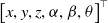
In Section 2, we transform the model identification problem into a multivariate linear regression problem. Genetic algorithms are introduced and combined with prediction networks to identify the required parameters. According to Griffiths [Reference Griffiths, Giannetti, Andrzejewski and Morgan35], the core operating mechanism of GA mainly includes two key genetic operators: crossover recombination and gene mutation. The crossover operation refers to the exchange and recombination of chromosome segments between two parent individuals at specific gene loci to produce new individuals. The mutation operation randomly selects specific gene loci in the individual chromosome and resets their values to valid random values within the value range space. The schematic diagram of the two operations is shown in Figure 2.

The algorithmic process includes generating a population, performing crossover and genetic operations on individuals in the population to generate new individuals, calculating the fitness of each individual according to the fitness function, and selecting the best n individuals to retain. If the required target is not achieved, the above process is repeated until the required target is met. In this paper, each individual contains four genes: $I_m'$ , $F_v'$ , $F_c'$ as well as $d_{\text{bios}}$ . According to (16), the fitness function is constructed:

(17) \begin{equation} f_{\text{fitness}} = \sum _{i=1}^n \left (a_{\text{low}}I_m^{\prime}+b_{\text{low}}F_{\!v}^{\prime}+c_{\text{low}}F_{\!c}^{\prime}+d_{\text{bias}}-U^*_{\text{low}}\right )^2, \end{equation}

where $d_{\text{bias}}$ stands for the fixed bias, which can be fitted by the TCN-Transformer network. At this point, we can present the framework of the entire identification algorithm, as shown in Figure 3.

Figure 3. Framework of system identification based on wavelet and TCN-transformer.

In most cases, obtaining the optimal system parameters requires a large amount of data. According to the trajectory prediction method proposed in Section 2, we can train a trajectory prediction system with a small amount of data and obtain a large amount of data through simulation to identify the optimal system parameters. Based on this, the overall framework of the method is constructed as follows: firstly, the TCN-Transformer model is trained using the collected small sample dataset to establish a virtual trajectory prediction system; secondly, the prediction system is used to generate high-quality virtual trajectories in batches; then, based on the generated virtual trajectory data, the identification method proposed in this study is used to construct a gray-box model of CDPRs; finally, the method proposed in this paper is verified and optimized using physical experimental data. Figure 4 is a schematic diagram of the overall framework.

Figure 4. Flowchart of overall framework.

In the next section, the feasibility and accuracy of this method will be demonstrated through experiments.

5. Simulation and experiments

5.1. Experimental equipment

To verify the performance advantages of the proposed method, experiments are conducted on a 3-DOF CDRS experimental platform, as shown in Figure 5. The CDPR system operates in a $3\ \mathrm{m}\times 3\ \mathrm{m}\times 2\ \mathrm{m}$ rectangular space and consists of a mobile robot platform and three sets of cable-driven components (including winches and guiding devices).

Figure 5. Three-degree-of-freedom CDPR.

This experiment also utilizes the Prime series high-precision motion capture system. Within the experimental space shown in Figure 6, 24 infrared optical capture cameras are evenly distributed according to the spatial geometry, forming a comprehensive three-dimensional tracking network. This enables comprehensive, all-around tracking and pose reconstruction of indoor moving targets. Each camera is equipped with an advanced CMOS sensor that has a resolution of 12 megapixels and a base frame rate of $300$ Hz, which can be increased to $1000$ Hz in high-speed mode, ensuring accurate capture of high-speed motion details. Through sub-pixel marker recognition and multi-camera joint solution technology, the system achieves a spatial positioning accuracy of 0.1 mm, an accuracy indicator verified by international standard metrology instruments.

Figure 6. Prime series high-precision motion capture system.

5.2. Data-driven trajectory generation experiment

To validate the effectiveness and accuracy of the proposed algorithm, we have collected a total of 200 experimental data sets during the normal operations of the CDPR. The trajectories contained in this data set are mainly divided into four categories: flat circle trajectories, oblique circle trajectories, flat Figure 7 trajectories, and oblique Figure 7 trajectories. Each category of trajectory contains 50 complete datasets. In this part of the experiment, we will use this dataset to train the TCN-Transformer network proposed in this paper, TCN, Transformer network, and the BiLSTM, which is widely used. Meanwhile, the mean squared error (MSE), the root mean squared error (RMSE), the MAE, the mean absolute percentage error (MAPE), R-Square ( $R^2$ ), and the proposed perplexity (PPL) will be calculated to measure the performance of these networks. After training, these networks will be tested on unknown trajectory generation to test their generalization performance.

The model input vector includes the time parameter $t$ , the desired position of the mobile platform at the current moment $x_{d}(t)$ , the measured position $x(t)$ , the real-time velocity $v(t)$ , the acceleration $a(t)$ , the rope length $l(t)$ , and the control input $u(t)$ . The output is the predicted value $x(t+1)$ of the platform’s position at the next moment. The experimental parameters are set as follows: TCN-Transformer, TCN, and Transformer all use a four-layer network architecture, trained for 300 cycles, with an initial learning rate set to 0.05 and an Adam optimizer; BiLSTM is configured with 256 hidden units, and the other hyperparameters remain unchanged. The number of attention heads in the Transformer framework is set to $16$ , the number of filters in the TCN is $5$ , whose width is $16$ , and the dropout factor is $10\%$ . 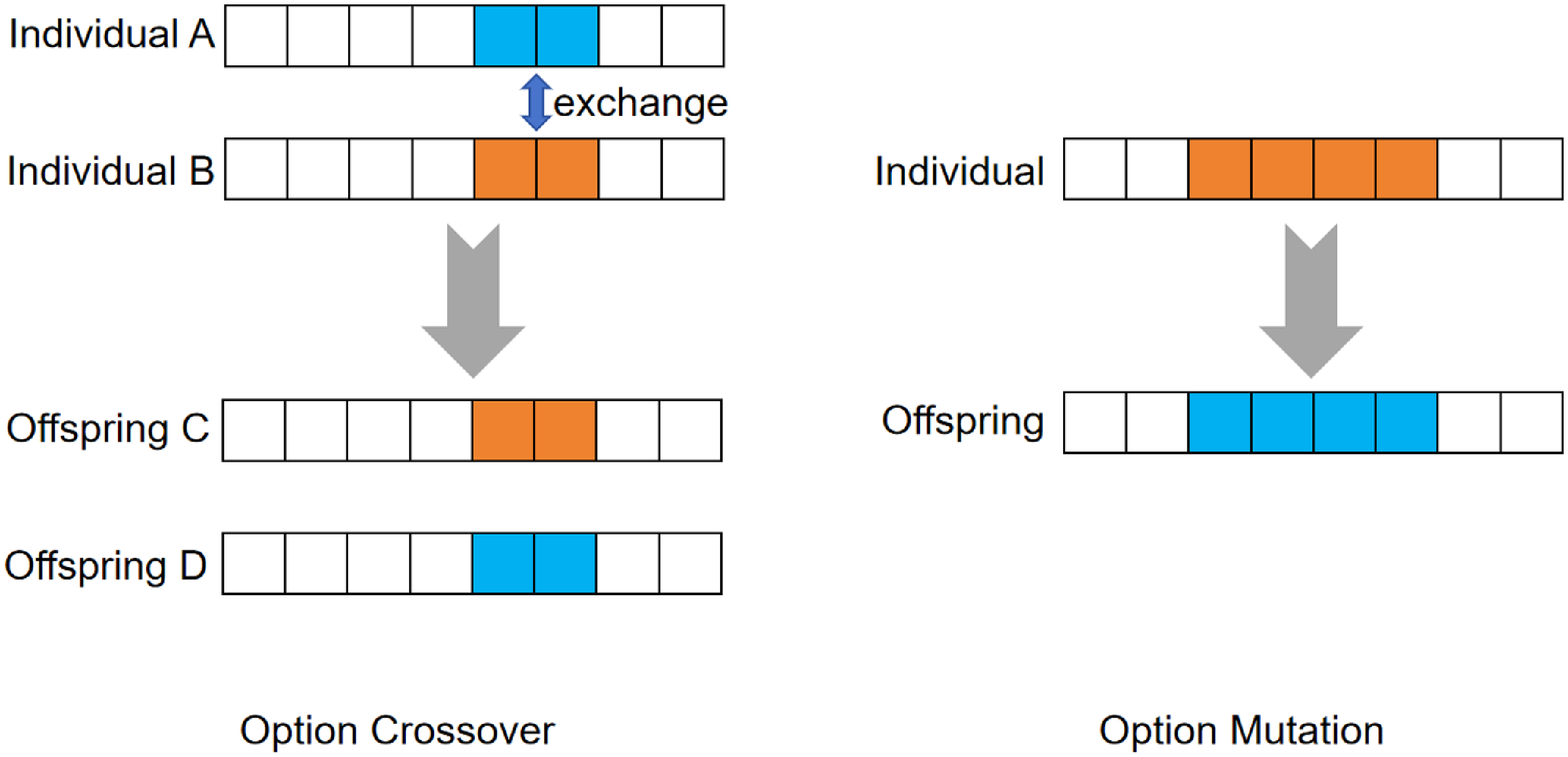Figure 8 shows the training errors of these networks, and Table I shows the values of related indicators.

Figure 7. The result of wavelet decomposition.

Based on the training set performance data in Table I, the TCN-Transformer network demonstrates comprehensive superiority in prediction accuracy, efficiency, and stability. Its core error metrics are significantly superior, with the x-axis MSE as low as $5.5637\times 10^{-6}$ (only $18.9\%$ of TCN’s) and the z-axis MAE as low as $1.5706\times 10^{-3}$ ( $30.9\%$ lower than the Transformer). Seven of the nine metrics used for evaluation were optimal. In particular, both the MSE and MAE were the lowest, $2.1\%$ and $28.2\%$ lower than the second-place Transformer, respectively. Training efficiency also achieved a significant improvement, completing training in just 88 s, a $43.2\%$ speedup compared to the Transformer ( $155\ s$ ) and a $32.8\%$ reduction compared to the BiLSTM ( $131\ s$ ), breaking the barrier that high-precision models often sacrifice speed. The model’s reliability was also double-checked: $R^2$ reaches $99.9914\%$ (surpassing the Transformer’s $99.9759\%$ ), demonstrating its strongest ability to model system dynamics. Furthermore, the perplexity PPL was lower than that of the comparison network on both the x/z axis and the average value, demonstrating the most concentrated distribution of prediction errors. In particular, compared to TCN and BiLSTM, this network, leveraging the local feature extraction capabilities of TCN temporal convolution and the global dependency modeling advantages of the Transformer, exhibits high accuracy, high efficiency, and strong stability.

Moreover, the values of MSE and RMSE can indeed reflect the overall degree of deviation between the predicted value and the actual data; however, the averaging algorithm may cause these indicators to ignore some details, such as the maximum and minimum values of the error. The data from the TCN-Transformer and the Transformer illustrate this conclusion. MAE and MAPE intuitively represent the gap between the predicted and the true value, but they do not take into account the variability of the target variable and may not accurately reflect the performance of the model. The PPL proposed in this paper can address the shortcomings of the aforementioned indicators. PPL not only reflects the overall degree of deviation but also indicates the magnitude of data fluctuation. The greater the fluctuation, the larger the PPL value.

Furthermore, these results demonstrate the high practicality of the proposed method. Firstly, to address the issues of high experimental costs, long experimental cycles, and aging losses, the method can utilize limited real data to generate large volumes of high-fidelity virtual data for parameter identification. This approach significantly shortens development cycles, reduces energy consumption, and minimizes equipment wear during testing, enabling rapid iteration and optimization. Secondly, high-quality trajectory prediction not only improves the accuracy of parameter identification but also provides a reliable model foundation for advanced control methods, enhancing both trajectory tracking precision and system stability.

Table I. Comparison of prediction results of training set.

Figure 8. The error of training set of four network structures. (a) TCN-transformer; (b) TCN; (c) Transformer; (d) LSTM.

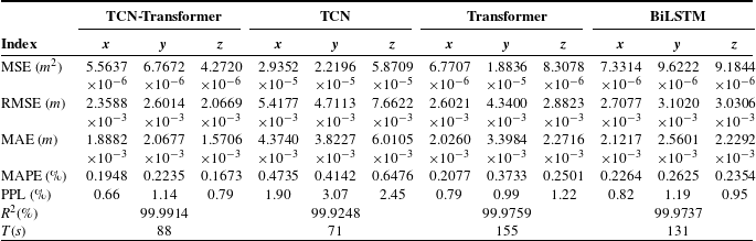
After training, we will use four trajectories to test the generalization ability of these networks: a flat circle, an oblique circle, an oblique 8 trajectory included in the training set, and a spiral trajectory that does not appear in the training set. The test results are shown in Table II.

Table II. Comparison of prediction results of test set.

According to the data in Table II, the TCN-Transformer network demonstrates significant advantages in performance and generalization. In known trajectory testing, its prediction accuracy surpasses that of all competing networks. For planar circular trajectories, the z-axis MSE is over $86\%$ lower than that of the Transformer and BiLSTM, and the z-axis MAE is $87\%$ higher than that of the BiLSTM. For oblique circular trajectories, the x-axis MSE is significantly better than that of the BiLSTM, while all three axes of the PPL are lower than those of other networks, demonstrating a more concentrated error distribution. For highly nonlinear oblique Figure 7 trajectories, the z-axis MAE is $21\%$ to $77\%$ lower than that of the TCN and BiLSTM, and the z-axis PPL is significantly lower than that of the BiLSTM, highlighting its robustness in modeling complex motion. Across 16 coordinate-trajectory combinations, this network achieves the lowest PPL in $75\%$ cases and maintains a leading position in 12 of these results.

In the unknown trajectory generalization test (spiral trajectories), the TCN-Transformer’s advantage further expanded: its x-axis MSE is $77\%$ lower than the best comparison network, the Transformer, while its y-axis MAE is $73\%$ higher than the BiLSTM. It maintained the lowest PPL on the z-axis and achieved an $R^2$ of $99.7396\%$ , significantly outperforming TCN. This demonstrates the network’s strong adaptability to untrained motion patterns. Its core advantages can be summarized in three key points: firstly, the TCN’s local feature extraction and the Transformer’s global dependency modeling capabilities achieved the lowest MSE/MAE in the test scenario; secondly, the innovative PPL metric verified its most stable prediction error distribution; and thirdly, key metrics outperformed the runner-up network by an average of over $35\%$ when faced with unknown spiral trajectories, demonstrating the architecture’s ability to capture high-frequency dynamic characteristics. These characteristics make it an ideal tool for parameter identification of complex systems, particularly in engineering scenarios requiring high-precision virtual trajectory generation.

The following will show the comparative analysis of experimental data and performance indicators between the traditional method and the intelligent identification method based on wavelet theory. Firstly, we show the results of wavelet decomposition in Figure 7. As mentioned in Section 4, the wavelet decomposition has two layers using the db4 wavelet as the base. Therefore, the original signal has been divided into three components: low-frequency components and high-frequency components from the first and second decompositions. As we can see from Figure 7, the frequency of the high-frequency components obtained from the first decomposition is significantly higher than that from the second. The obtained low-frequency components were used to identify system parameters, while the decomposed high-frequency components were used for fitting by the TCN-Transformer.

The identification values of relevant system parameters are provided by two methods based on the measured data:

\begin{equation*} \begin{split} \boldsymbol{M} &= \text{diag}(2,2,2)(kg),\\ \boldsymbol{R}&=\text{diag}(0.06,0.06,0.06). \end{split} \end{equation*}

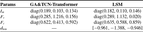
Based on the constructed dataset and the virtual dataset generated by the trajectory prediction method, the system parameter comparison results obtained by this research method and the traditional method (traditional least squares method, LSM) are shown in Table III.

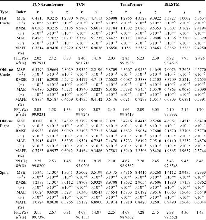
Table III. Comparison of prediction results of spiral trajectory on test sets.

According to the data in Table III, it is found that the system parameters of the x-axis identified by the two methods are almost the same, $F_c$ of the y-axis is significantly different, and $F_v$ and $F_c$ of the z-axis are significantly different. In order to further evaluate the advantages and disadvantages of the two methods, data reconstruction and visualization analysis are carried out based on the helical trajectory results from the aforementioned trajectory prediction and the parameter identification results. Due to space limitations, this paper only shows the reconstruction curve under the condition of $i=1$ , as shown in Figure 9.

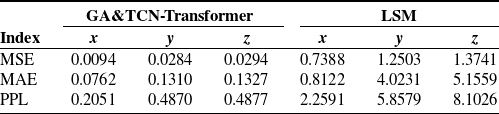
The error metrics, including MSE, MAE, and PPL, associated with the two methods are shown in Table IV.

The comparative analysis in Figure 9 shows that the traditional parameter identification method has significant deviations, while the proposed improved algorithm has significant advantages in parameter identification accuracy, and its residual range converges to the interval $[-0.207, 0.470]$ . Comparing the data in Table IV, it can be found that the three indicators of the proposed method are superior to those of LSM. Especially in the PPL index, the value of the new method is much lower than that of LSM. This shows that the traditional methods are not able to deal with high-frequency components and noise, leading to an underestimation of the friction effect. Through wavelet enhancement and genetic algorithm optimization, the new method can more comprehensively characterize the high-frequency dynamics of the system, especially the friction nonlinearity.

It should be pointed out that although the parameter identification accuracy is improved, the signal reconstruction error is still maintained at a high level due to the inherent structure of the model, which suggests that subsequent research needs to optimize the structure of the model described in Chapter 2. Substitute the optimized parameters into the identification framework proposed in this paper, dynamically identify the system disturbance $d$ through TCN-Transformer, and implement signal reconstruction based on Eq. (1). The reconstruction effect verification is shown in Figure 7.

Table IV. Comparison of signal reconstruction results.

Figure 9. Comparison between TCN-transformer and LSM. (a) Signal. (b) Error.

The error ranges between the three-axis reconstructed signal and the original signal are $[\!-0.3294,0.3206]$ , $[-0.7967, 0.6641]$ and $[-0.5372, 0.9366]$ respectively. The analysis results show that the parameter identification method proposed in this study can accurately obtain the system dynamic parameters $\boldsymbol{I}_m$ , $\boldsymbol{F}_v$ , and $\boldsymbol{F}_c$ , and realize the dynamic prediction of the system disturbance $\boldsymbol{d}$ .

Applying the above results to the actual dataset, the result of one oblique circle trajectory is shown in Table V.

Table V. The results of applying simulation results to actual trajectories.

Figure 10. Comparison of the signal reconstructed by the new method with the original signal.

Figure 10 illustrates the comparison between the calculated results and the original signal, and Table V gives the index values. Thus, t we can draw a conclusion that the identification results calculated by the previously constructed virtual trajectory can still achieve a good fitting effect when applied to the actual trajectory.