


1. Introduction
Capsules, consisting of a liquid core surrounded by a membrane, are common in both nature (e.g. cells) and bioengineering applications (Pozrikidis Reference Pozrikidis2003b ). Since the membrane is elastic, it deforms under flow. Due to the possibility of breakup, there is interest in mechanical modelling of deformation (Barthés-Biesel Reference Barthés-Biesel2016). In particular, the desire to characterise the mechanical properties of cell membranes has led to the development of deformability cytometry (Mietke et al. Reference Mietke, Otto, Girardo, Rosendahl, Taubenberger, Golfier, Ulbricht, Aland, Guck and Fischer-Friedrich2015; Otto et al. Reference Otto2015; Rosendahl et al. Reference Rosendahl2018), where cells are subject to shearing flow in microfluidic devices, with their deformation being recorded by high-speed cameras.
It is common to model the thin membrane by a two-dimensional surface with an elastic constitutive law that introduces resistance to shear and area dilatation, but not to bending. The canonical problem involves the specification of simple shear flow, under which the membrane deforms. More generally, other types of linear flows have been considered, in particular two-dimensional elongational flow and axially symmetric hyperbolic flow. In these flows, the capsule shape can reach a steady state (which is unattainable under simple shear). For that reason, such flows are convenient for experimental observations and possibly for characterising material response (Chang & Olbricht Reference Chang and Olbricht1993). With a steady state, moreover, the internal liquid is stationary, so its viscosity does not play a role.
The deformed shape of the membrane is determined by static equilibrium, where the hydrodynamic tractions are balanced by the (surface divergence of the) elastic stresses. There is a fundamental difference in determining the hydrodynamic and elastic forces. The hydrodynamic problem, and in particular the resulting traction, is determined by the deformed shape alone. The elastic stresses are set by the deformation from a given reference (typically spherical) shape to the present shape. The theoretical calculation of capsule deformation falls under the broader framework of fluid–structure interactions (Dowell & Hall Reference Dowell and Hall2001). Given the typical small size of capsules (e.g. approximately 10 μm for a red blood cell), inertia is typically negligible; the flow is therefore governed by the Stokes equations.
Modelling the elastic response to deformation requires a constitutive law for the stresses. The neo-Hookean law, a particular case of the Mooney–Rivlin law, constitutes the thin limit of an incompressible solid; it appropriately describes rubber-like materials. Another common model is the Skalak law (Skalak et al. Reference Skalak, Tozeren, Zarda and Chien1973), an isotropic two-dimensional model with independent surface shear and area dilatation moduli that was specifically designed to model red blood cells. Both constitutive descriptions are nonlinear. With the deformed shape itself being unknown, the equilibrium problem is inherently nonlinear.
The key parameter governing the dimensionless problem is the elastic capillary number $Ca$
, representing the characteristic ratio of viscous stresses to elastic stresses. Initial investigations (Barthés-Biesel Reference Barthés-Biesel1980; Barthés-Biesel & Rallison Reference Barthés-Biesel and Rallison1981) considered the stiff limit
$Ca$
, representing the characteristic ratio of viscous stresses to elastic stresses. Initial investigations (Barthés-Biesel Reference Barthés-Biesel1980; Barthés-Biesel & Rallison Reference Barthés-Biesel and Rallison1981) considered the stiff limit ${Ca}\ll 1$
, where the membrane deforms only slightly. Given the interest in significant deformations, these were later supplemented by numerical simulations at finite values of
${Ca}\ll 1$
, where the membrane deforms only slightly. Given the interest in significant deformations, these were later supplemented by numerical simulations at finite values of $Ca$
(Li, Barthés-Biesel & Helmy Reference Li, Barthés-Biesel and Helmy1988; Pozrikidis Reference Pozrikidis1990, Reference Pozrikidis2003a
; Dodson III & Dimitrakopoulos Reference Dodson and Dimitrakopoulos2008, Reference Dodson and Dimitrakopoulos2009). The ultimate goal of the theoretical analysis is the calculation of the capsule deformation; representing it by appropriate lumped scalar measures, it is desirable to understand how they vary as a function of
$Ca$
(Li, Barthés-Biesel & Helmy Reference Li, Barthés-Biesel and Helmy1988; Pozrikidis Reference Pozrikidis1990, Reference Pozrikidis2003a
; Dodson III & Dimitrakopoulos Reference Dodson and Dimitrakopoulos2008, Reference Dodson and Dimitrakopoulos2009). The ultimate goal of the theoretical analysis is the calculation of the capsule deformation; representing it by appropriate lumped scalar measures, it is desirable to understand how they vary as a function of $Ca$
.
$Ca$
.
At large $Ca$
the capsule undergoes large deformation whose nature, as observed numerically, depends critically on the elastic behaviour. For certain constitutive laws, the most notable being neo-Hookean, there exists a critical capillary number beyond which no steady shape is attained under elongation (Li et al. Reference Li, Barthés-Biesel and Helmy1988). For that reason the neo-Hookean law is classified as ‘strain softening’. For ‘strain hardening’ laws, such as the Skalak description, the capsule does attain a steady slender shape for large
$Ca$
the capsule undergoes large deformation whose nature, as observed numerically, depends critically on the elastic behaviour. For certain constitutive laws, the most notable being neo-Hookean, there exists a critical capillary number beyond which no steady shape is attained under elongation (Li et al. Reference Li, Barthés-Biesel and Helmy1988). For that reason the neo-Hookean law is classified as ‘strain softening’. For ‘strain hardening’ laws, such as the Skalak description, the capsule does attain a steady slender shape for large $Ca$
(Li et al. Reference Li, Barthés-Biesel and Helmy1988; Barthès-Biesel et al. Reference Barthès-Biesel, Diaz and Dhenin2002; Walter et al. Reference Walter, Salsac, Barthès-Biesel and Le Tallec2010). In fact, numerical computations (Dodson III & Dimitrakopoulos Reference Dodson and Dimitrakopoulos2008, Reference Dodson and Dimitrakopoulos2009) reveal slender shapes even at moderately large capillary numbers,
$Ca$
(Li et al. Reference Li, Barthés-Biesel and Helmy1988; Barthès-Biesel et al. Reference Barthès-Biesel, Diaz and Dhenin2002; Walter et al. Reference Walter, Salsac, Barthès-Biesel and Le Tallec2010). In fact, numerical computations (Dodson III & Dimitrakopoulos Reference Dodson and Dimitrakopoulos2008, Reference Dodson and Dimitrakopoulos2009) reveal slender shapes even at moderately large capillary numbers, ${Ca}\approx 2.5$
.
${Ca}\approx 2.5$
.
Motivated by the interest in large deformation (Eggleton & Popel Reference Eggleton and Popel1998; Navot Reference Navot1998; Ramanujan & Pozrikidis Reference Ramanujan and Pozrikidis1998) we conduct here an asymptotic investigation in the limit ${Ca}\gg 1$
. Our key goal is to determine the asymptotic dependence of the slenderness
${Ca}\gg 1$
. Our key goal is to determine the asymptotic dependence of the slenderness $\epsilon$
upon
$\epsilon$
upon $Ca$
. For simplicity we consider uniaxial extensional flow, where the problem is axially symmetric, and seek the steady shape attained by the capsule.
$Ca$
. For simplicity we consider uniaxial extensional flow, where the problem is axially symmetric, and seek the steady shape attained by the capsule.
In classical slender-body analyses about rigid bodies (Batchelor Reference Batchelor1970; Cox Reference Cox1970) the slenderness $\epsilon \ll 1$
is prescribed in the problem formulation. A key challenge in the present problem is that the slenderness is unknown to begin with, and is in fact a part of the problem. In that sense, our problem is reminiscent of bubble deformation (Buckmaster Reference Buckmaster1972, Reference Buckmaster1973; Acrivos & Lo Reference Acrivos and Lo1978; Sherwood Reference Sherwood1981). It is, however, significantly more complicated. The free surface in the bubble problem is characterised by a uniform surface tension; consequently, its mechanical model is expressed via an internal force that acts normal to the surface. The membrane of a capsule is described by more elaborate mechanics that result in both normal and tangential internal forces. In that aspect, the present problem is closer to that describing a bubble whose boundary is contaminated by surfactants (Booty & Siegel Reference Booty and Siegel2005). Another challenge we face, which seems new in slender-body analyses, has to do with the conflict between the ‘Lagrangian’ description required for the calculation of the elastic stress and the ‘Eulerian’ description required for the hydrodynamic formulation.
$\epsilon \ll 1$
is prescribed in the problem formulation. A key challenge in the present problem is that the slenderness is unknown to begin with, and is in fact a part of the problem. In that sense, our problem is reminiscent of bubble deformation (Buckmaster Reference Buckmaster1972, Reference Buckmaster1973; Acrivos & Lo Reference Acrivos and Lo1978; Sherwood Reference Sherwood1981). It is, however, significantly more complicated. The free surface in the bubble problem is characterised by a uniform surface tension; consequently, its mechanical model is expressed via an internal force that acts normal to the surface. The membrane of a capsule is described by more elaborate mechanics that result in both normal and tangential internal forces. In that aspect, the present problem is closer to that describing a bubble whose boundary is contaminated by surfactants (Booty & Siegel Reference Booty and Siegel2005). Another challenge we face, which seems new in slender-body analyses, has to do with the conflict between the ‘Lagrangian’ description required for the calculation of the elastic stress and the ‘Eulerian’ description required for the hydrodynamic formulation.
In analysing the deformation problem at large $Ca$
it is necessary to allow for cusped ends. The transition from spindled-to-cusped edges was originally observed in experiments (Barthés-Biesel Reference Barthés-Biesel1991) using a four-roller apparatus (e.g. Bentley & Leal Reference Bentley and Leal1986). In fact, the inability of ‘state of the art’ computation schemes (at that time) to reach large capillary numbers, beyond that transition, motivated the use of spectral boundary-element algorithms (Wang & Dimitrakopoulos Reference Wang and Dimitrakopoulos2006; Dodson III & Dimitrakopoulos Reference Dodson and Dimitrakopoulos2008) that do predict cusped ends. In our asymptotic analysis, we allow for pointed ends at the very outset. This affects the boundary conditions governing the deformed shape.
$Ca$
it is necessary to allow for cusped ends. The transition from spindled-to-cusped edges was originally observed in experiments (Barthés-Biesel Reference Barthés-Biesel1991) using a four-roller apparatus (e.g. Bentley & Leal Reference Bentley and Leal1986). In fact, the inability of ‘state of the art’ computation schemes (at that time) to reach large capillary numbers, beyond that transition, motivated the use of spectral boundary-element algorithms (Wang & Dimitrakopoulos Reference Wang and Dimitrakopoulos2006; Dodson III & Dimitrakopoulos Reference Dodson and Dimitrakopoulos2008) that do predict cusped ends. In our asymptotic analysis, we allow for pointed ends at the very outset. This affects the boundary conditions governing the deformed shape.
Following the numerical classification of strain softening and strain hardening materials, we employ here the Skalak model which was numerically observed to result in steady-state large deformation. Indeed, it seems that the Skalak model has become the de facto constitutive description for capsules in the literature (Dodson III & Dimitrakopoulos Reference Dodson and Dimitrakopoulos2008, Reference Dodson and Dimitrakopoulos2009). We also briefly discuss the strain softening neo-Hookean model, which was numerically observed to burst under strong flows.
2. Problem formulation
2.1. Physical problem
A capsule is made of a liquid core and an elastic encapsulating membrane, whose reference shape is spherical, say of radius $R$
. The thin membrane is described by an effective two-dimensional elasticity which represents resistance to shear (captured by the modulus
$R$
. The thin membrane is described by an effective two-dimensional elasticity which represents resistance to shear (captured by the modulus $G$
) and area dilatation (captured by the modulus
$G$
) and area dilatation (captured by the modulus $K$
), but no resistance to bending. The two material coefficients have the dimensions of surface tension, i.e. force per unit length.
$K$
), but no resistance to bending. The two material coefficients have the dimensions of surface tension, i.e. force per unit length.
The capsule is suspended in a viscous liquid of viscosity $\mu$
and is exposed to a uniaxial extensional flow of extension rate
$\mu$
and is exposed to a uniaxial extensional flow of extension rate $E$
. The capsule reaches a steady shape whose symmetry axis is aligned with the axis of extension. The capsule length along that axis is denoted by
$E$
. The capsule reaches a steady shape whose symmetry axis is aligned with the axis of extension. The capsule length along that axis is denoted by $2L$
; its ‘waist’ radius in the midway symmetry plane is denoted by
$2L$
; its ‘waist’ radius in the midway symmetry plane is denoted by $\epsilon L$
. Our interest is in the evaluation of the geometric parameters
$\epsilon L$
. Our interest is in the evaluation of the geometric parameters $\epsilon$
and
$\epsilon$
and $L/R$
, which quantify the overall deformation. By dimensional arguments, these parameters can only depend upon the two dimensionless parameters of the problem, namely
$L/R$
, which quantify the overall deformation. By dimensional arguments, these parameters can only depend upon the two dimensionless parameters of the problem, namely $K/G$
and the elastic capillary number
$K/G$
and the elastic capillary number
 \begin{equation} {Ca} = \frac {\mu R E}{G}, \end{equation}
which expresses the relative magnitude of viscous and elastic stresses. Once the capsule reaches a steady shape, its core liquid is stationary. The ratio of the core viscosity to the external-liquid viscosity – a third dimensionless parameter which affects the transient problem – is accordingly irrelevant.
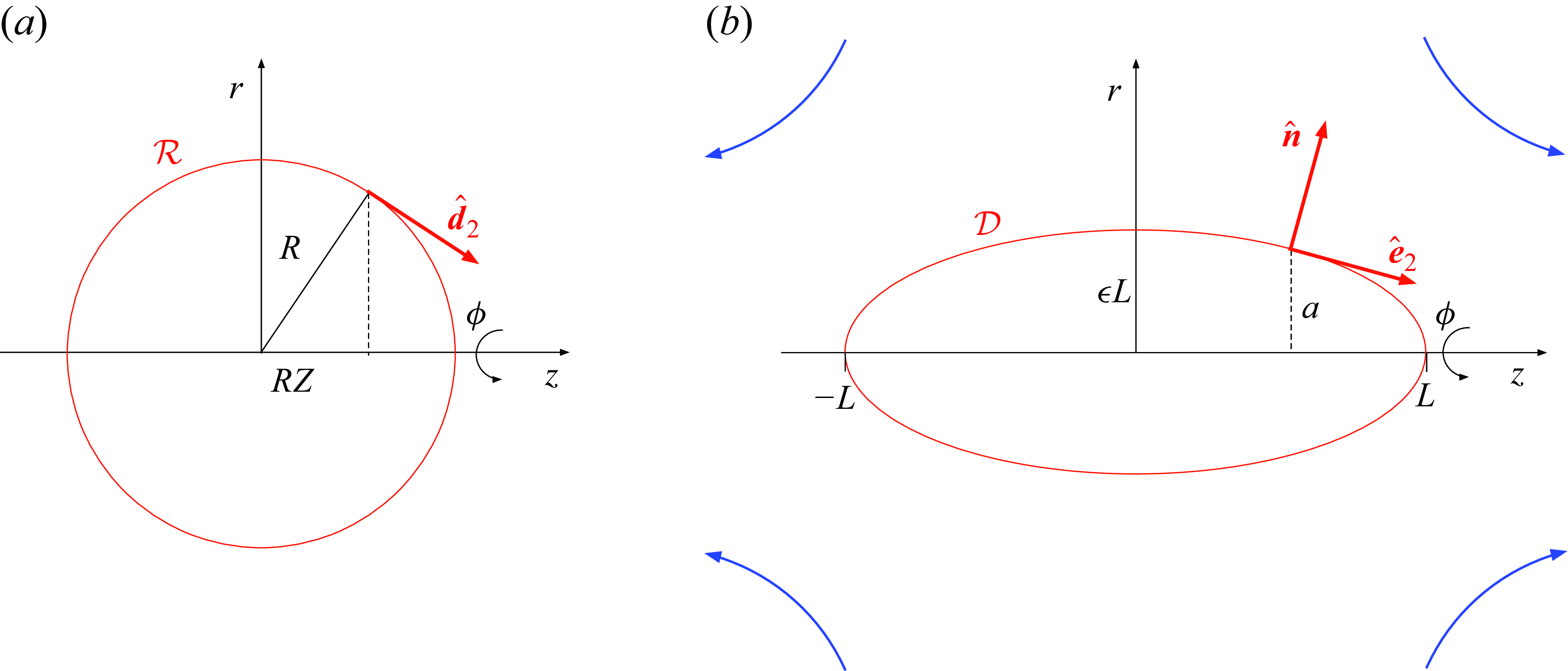
2.2. Geometry
We employ cylindrical $({r},\phi,z)$
coordinates with the
$({r},\phi,z)$
coordinates with the $z$
-axis coinciding with axis of symmetry and
$z$
-axis coinciding with axis of symmetry and $z=0$
coinciding with the symmetry plane of the extensional flow. We write the shape of the deformed membrane
$z=0$
coinciding with the symmetry plane of the extensional flow. We write the shape of the deformed membrane $\mathcal D$
as
$\mathcal D$
as
 \begin{equation} {r} = a(z), \end{equation}
see figure 1. Since the deformed shape is symmetric about the plane $z=0$
,
$z=0$
, $a$
is an even function:
$a$
is an even function: $a(-z)= a(z)$
. By definition,
$a(-z)= a(z)$
. By definition,
 \begin{equation} a(\pm L)=0. \end{equation}
Given the definition of $\epsilon$
, the shape function also satisfies
$\epsilon$
, the shape function also satisfies
 \begin{equation} a(0) = \epsilon L. \end{equation}
Since the capsule core is incompressible, volume conservation gives the constraint
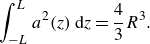 \begin{equation} \int _{-L}^L a^2(z)\,\mathrm{d} z=\frac {4}{3}R^3. \end{equation}
Schematic of the reference (a) and deformed (b) geometries.
Using $z$
and
$z$
and $\phi$
for parametrisation, the position vector pointing to the deformed membrane
$\phi$
for parametrisation, the position vector pointing to the deformed membrane $\mathcal D$
is
$\mathcal D$
is
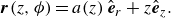 \begin{equation} \boldsymbol{r}(z,\phi)=a(z)\,\hat {\boldsymbol{e}}_r + z\hat {\boldsymbol{e}}_z. \end{equation}
By differentiating (2.6) we obtain
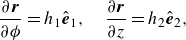 \begin{align} \frac {\partial \boldsymbol{r}}{\partial \phi }=h_1\hat {\boldsymbol{e}}_1, \quad \frac {\partial \boldsymbol{r}}{\partial z}=h_2\hat {\boldsymbol{e}}_2, \end{align}
where the associated basis vectors and corresponding scale factors are
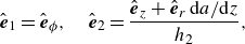 \begin{align} \hat{\boldsymbol{e}}_1=\hat{\boldsymbol{e}}_\phi, \quad\hat{\boldsymbol{e}}_2=\frac{\hat{\boldsymbol{e}}_z+\hat{\boldsymbol{e}}_r\, {\text{d} a}/{\text{d} z}}{h_2},\end{align}
and
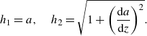 \begin{align} h_1=a, \quad h_2=\sqrt {1 + \left(\dfrac{\mathrm{d} a}{\mathrm{d} z} \right)^2}. \end{align}
The (outward-pointing) unit normal is therefore given by
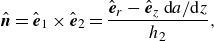 \begin{equation} \hat {\boldsymbol{n}}=\hat {\boldsymbol{e}}_1\times \hat {\boldsymbol{e}}_2 =\frac {\hat {\boldsymbol{e}}_r-\hat {\boldsymbol{e}}_z\, {\mathrm{d} a}/{\mathrm{d} z}}{h_2}, \end{equation}
see figure 1.
2.3. Deformation
In principle, the prescription of the deformation from the reference shape $\mathcal R$
to the deformed shape
$\mathcal R$
to the deformed shape $\mathcal D$
requires: (i) parametrisation of
$\mathcal D$
requires: (i) parametrisation of $\mathcal R$
using two variables and (ii) mapping each point on
$\mathcal R$
using two variables and (ii) mapping each point on $\mathcal R$
to a point in
$\mathcal R$
to a point in $\mathcal D$
. Due to the axial symmetry this requires two functions, providing the axial and radial coordinates of the mapped point. Recalling that
$\mathcal D$
. Due to the axial symmetry this requires two functions, providing the axial and radial coordinates of the mapped point. Recalling that $\mathcal R$
is a sphere of radius
$\mathcal R$
is a sphere of radius $R$
, each point on it is parametrised using its azimuthal coordinate
$R$
, each point on it is parametrised using its azimuthal coordinate $\phi$
and its
$\phi$
and its $z$
-coordinate, say
$z$
-coordinate, say $RZ$
(
$RZ$
( $Z\in [-1,1]$
). The two aforementioned functions, which depend only upon
$Z\in [-1,1]$
). The two aforementioned functions, which depend only upon $Z$
, are represented by the mappings
$Z$
, are represented by the mappings
 \begin{align} Z\mapsto z, \quad Z\mapsto r. \end{align}
While this procedure may be suitable to numerical solutions, it does not merge with the eventual need to perform an asymptotic analysis in the slender limit. For example, in analysing the flow problem the natural parametrisation is expressed in the context of the deformed shape.
This incompatibility is resolved using a parametrisation in $\mathcal D$
in conjunction with the inverse of (2.11a
). To that end, we denote the preimage of
$\mathcal D$
in conjunction with the inverse of (2.11a
). To that end, we denote the preimage of $z$
as
$z$
as $Z(z)$
. The function
$Z(z)$
. The function $a(z)$
, introduced in the previous subsection, is formally constructed by the composition of
$a(z)$
, introduced in the previous subsection, is formally constructed by the composition of $Z(z)$
with (2.11b
).
$Z(z)$
with (2.11b
).
It is evident that $Z(z)$
is an odd function that satisfies
$Z(z)$
is an odd function that satisfies
 \begin{equation} Z(\pm L)=\pm 1. \end{equation}
It is tempting to add a condition representing the extrema attained by (2.11a
) at the two ‘ends’ of the capsule. In terms of the mapping $Z(z)$
, this gives
$Z(z)$
, this gives
 \begin{equation} \lim _{|z|\nearrow L} \frac {\sqrt {1-Z}}{{\mathrm{d}{Z}}/{\mathrm{d}{z}}} = 0. \end{equation}
However, given the anticipation of a cusped-end, we avoid that ‘spindle-end’ condition which only holds for smooth ends. We will provide later the appropriate condition replacing (2.13).
Consider now the deformation of a line element corresponding to infinitesimal increments $(\mathrm{d}\phi,\mathrm{d} z)$
. The deformation displaces a point with ‘initial’ position
$(\mathrm{d}\phi,\mathrm{d} z)$
. The deformation displaces a point with ‘initial’ position
 \begin{equation} \boldsymbol{R}(z,\phi)=\hat {\boldsymbol{e}}_r R\sqrt {1-Z^2(z)} + \hat {\boldsymbol{e}}_zRZ(z) \end{equation}
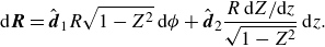
to the ‘new’ position (2.6). Upon differentiating (2.14) we find that
 \begin{equation} \mathrm{d}\boldsymbol{R}=\hat {\boldsymbol{e}}_\phi R\sqrt {1-Z^2}\,\mathrm{d}\phi + \left (\hat {\boldsymbol{e}}_z-\frac {Z}{\sqrt {1-Z^2}}\,\hat {\boldsymbol{e}}_r\right)R\frac {\mathrm{d} {Z}}{\mathrm{d} {z}}\,\mathrm{d} z. \end{equation}
Noting that the two basis vectors in $\mathcal R$
are (see figure 1)
$\mathcal R$
are (see figure 1)
 \begin{equation} \hat {\boldsymbol{d}}_1=\hat {\boldsymbol{e}}_\phi, \quad \hat {\boldsymbol{d}}_2= \hat {\boldsymbol{e}}_z \sqrt {1-Z^2} - \hat {\boldsymbol{e}}_r Z, \end{equation}
we find that
 \begin{equation} \mathrm{d}\boldsymbol{R}=\hat {\boldsymbol{d}}_1R\sqrt {1-Z^2}\,\mathrm{d}\phi +\hat {\boldsymbol{d}}_2\frac {R\,{\mathrm{d} Z}/{\mathrm{d} z}}{\sqrt {1-Z^2}}\,\mathrm{d} z. \end{equation}
Since (2.7) gives
 \begin{equation} \mathrm{d}\boldsymbol{r}=\hat {\boldsymbol{e}}_1h_1\,\mathrm{d}\phi + \hat {\boldsymbol{e}}_2h_2\,\mathrm{d} z, \end{equation}
we can read off the principal stretches, namely
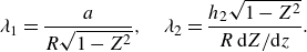 \begin{align} \lambda _1=\frac {a}{R\sqrt {1-Z^2}}, \quad \lambda _2=\frac {h_2\sqrt {1-Z^2}}{R\,{\mathrm{d} Z}/{\mathrm{d} z}}. \end{align}
Note that $\lambda _1$
is the ratio of the deformed radius
$\lambda _1$
is the ratio of the deformed radius $a(z)$
to the reference radius at
$a(z)$
to the reference radius at $Z(z)$
, see (2.14).
$Z(z)$
, see (2.14).
2.4. Flow
Consider now the flow field in the membrane exterior, where the velocity field is denoted by $\boldsymbol{u}$
and the associated stress tensor by
$\boldsymbol{u}$
and the associated stress tensor by $\boldsymbol{\sigma }$
. The flow is governed by the continuity and Stokes equations,
$\boldsymbol{\sigma }$
. The flow is governed by the continuity and Stokes equations,
 \begin{align} \boldsymbol{\nabla }\boldsymbol{\cdot }\boldsymbol{u}=0, \quad \boldsymbol{\nabla }\boldsymbol{\cdot }\boldsymbol{\sigma } = \boldsymbol{0}. \end{align}
At the deformed membrane it satisfies the no-slip condition,
 \begin{equation} \boldsymbol{u}=\boldsymbol{0} \quad \text{for} \quad r=a(z), \end{equation}
while at large distances it approaches the imposed flow
 \begin{equation} \boldsymbol{u}\sim E\left (z\hat {\boldsymbol{e}}_z-\frac {r}{2}\hat {\boldsymbol{e}}_{r}\right) \quad \text{as} \quad r^2 + z^2\to \infty. \end{equation}
As this is the same problem governing the flow outside a rigid body, the flow is uniquely determined by the shape of the deformed capsule, as provided by the distribution $a(z)$
. Since the interior fluid is stationary, the stress there is isotropic, say
$a(z)$
. Since the interior fluid is stationary, the stress there is isotropic, say $-P{I}$
.
$-P{I}$
.
For an incompressible flow, the pressure field is generally defined to within an arbitrary additive constant; since the pressure difference across the membrane is physically meaningful, this arbitrariness may only be exploited once, either in the membrane interior or its exterior. With no loss of generality, we set the pressure at infinity to zero, The constant $P$
thereby represents the difference between the uniform interior pressure and the far-field pressure in the exterior region. With that choice, the magnitude of both
$P$
thereby represents the difference between the uniform interior pressure and the far-field pressure in the exterior region. With that choice, the magnitude of both $\boldsymbol{\sigma }$
and
$\boldsymbol{\sigma }$
and $P$
is proportional to
$P$
is proportional to $\mu E$
; in particular,
$\mu E$
; in particular, $P$
may be interpreted as a ‘dynamic’ pressure.
$P$
may be interpreted as a ‘dynamic’ pressure.
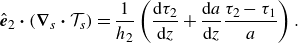
Due to axial symmetry, the velocity must be of the form
 \begin{equation} \boldsymbol{u} = \hat {\boldsymbol{e}}_r u + \hat {\boldsymbol{e}}_z w, \end{equation}
where $u$
and
$u$
and $w$
are functions of
$w$
are functions of $r$
and
$r$
and $z$
, but not of
$z$
, but not of $\phi$
. Consequently, the Newtonian stress must be of the form
$\phi$
. Consequently, the Newtonian stress must be of the form
 \begin{equation} \boldsymbol{\sigma } = \hat {\boldsymbol{e}}_r\hat {\boldsymbol{e}}_r \sigma _{rr} + \hat {\boldsymbol{e}}_z\hat {\boldsymbol{e}}_z \sigma _{zz} + (\hat {\boldsymbol{e}}_r\hat {\boldsymbol{e}}_z + \hat {\boldsymbol{e}}_z\hat {\boldsymbol{e}}_r) \sigma _{rz}, \end{equation}
where $\sigma _{rr}$
,
$\sigma _{rr}$
, $\sigma _{zz}$
and
$\sigma _{zz}$
and $\sigma _{rz}$
are functions of
$\sigma _{rz}$
are functions of $r$
and
$r$
and $z$
.
$z$
.
2.5. Static equilibrium
The shape $\mathcal D$
of the deformed membrane is governed by the force balance
$\mathcal D$
of the deformed membrane is governed by the force balance
 \begin{equation} \boldsymbol{\nabla }_s \boldsymbol{\cdot } \mathcal{T}_s + \hat {\boldsymbol{n}} \boldsymbol{\cdot } \boldsymbol{\sigma } + \hat {\boldsymbol{n}} P = \boldsymbol{0} \quad \text{at} \quad {r} = a(z), \end{equation}
applying for $-L\lt z\lt L$
, where
$-L\lt z\lt L$
, where $\boldsymbol{\nabla }_s$
is the surface-gradient operator and
$\boldsymbol{\nabla }_s$
is the surface-gradient operator and $\mathcal{T}_s$
the surface stress. By forming the dot product of (2.25) with
$\mathcal{T}_s$
the surface stress. By forming the dot product of (2.25) with $\hat {\boldsymbol{e}}_2$
we obtain the meridional balance
$\hat {\boldsymbol{e}}_2$
we obtain the meridional balance
 \begin{equation} \hat {\boldsymbol{e}}_2 \boldsymbol{\cdot } (\boldsymbol{\nabla }_s \boldsymbol{\cdot } \mathcal{T}_s) + \hat {\boldsymbol{n}} \boldsymbol{\cdot } \boldsymbol{\sigma } \boldsymbol{\cdot } \hat {\boldsymbol{e}}_2=0. \end{equation}
Similarly, by forming the dot product of (2.25) with $\hat {\boldsymbol{n}}$
we obtain the normal balance
$\hat {\boldsymbol{n}}$
we obtain the normal balance
 \begin{equation} \hat {\boldsymbol{n}} \boldsymbol{\cdot } (\boldsymbol{\nabla }_s \boldsymbol{\cdot } \mathcal{T}_s) + \hat {\boldsymbol{n}} \boldsymbol{\cdot } \boldsymbol{\sigma } \boldsymbol{\cdot } \hat {\boldsymbol{n}} + P=0. \end{equation}
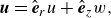
It is evident from the problem symmetry that the principal directions of the Cauchy tension $\mathcal{T}_s$
are provided by the unit vectors (2.8). We therefore write the Cauchy tension in the form
$\mathcal{T}_s$
are provided by the unit vectors (2.8). We therefore write the Cauchy tension in the form
 \begin{equation} \mathcal{T}_s = \tau _1\hat {\boldsymbol{e}}_1\hat {\boldsymbol{e}}_1 + \tau _2\hat {\boldsymbol{e}}_2\hat {\boldsymbol{e}}_2. \end{equation}
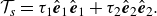
The component of $\boldsymbol{\nabla }_s \boldsymbol{\cdot } \mathcal{T}_s$
in the meridional direction is
$\boldsymbol{\nabla }_s \boldsymbol{\cdot } \mathcal{T}_s$
in the meridional direction is
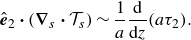
 \begin{equation} \hat {\boldsymbol{e}}_2 \boldsymbol{\cdot } (\boldsymbol{\nabla }_s \boldsymbol{\cdot } \mathcal{T}_s) = \frac {\mathrm{d} {\tau _2}}{\mathrm{d} {s}} + \frac {1}{a}\frac {\mathrm{d} {a}}{\mathrm{d} {s}}(\tau _2-\tau _1), \end{equation}
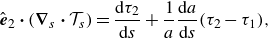
wherein $s$
is the arclength in the meridional plane, increasing in the direction of
$s$
is the arclength in the meridional plane, increasing in the direction of $\hat {\boldsymbol{e}}_2$
; making use of (2.7b
) yields
$\hat {\boldsymbol{e}}_2$
; making use of (2.7b
) yields
 \begin{equation} \hat {\boldsymbol{e}}_2 \boldsymbol{\cdot } (\boldsymbol{\nabla }_s \boldsymbol{\cdot } \mathcal{T}_s) =\frac {1}{h_2}\left (\frac {\mathrm{d} {\tau _2}}{\mathrm{d} {z}} + \frac {\mathrm{d} {a}}{\mathrm{d} {z}}\frac {\tau _2-\tau _1}{a}\right). \end{equation}
The component of $\boldsymbol{\nabla }_s \boldsymbol{\cdot } \mathcal{T}_s$
in the normal direction is
$\boldsymbol{\nabla }_s \boldsymbol{\cdot } \mathcal{T}_s$
in the normal direction is
 \begin{equation} \hat {\boldsymbol{n}} \boldsymbol{\cdot } (\boldsymbol{\nabla }_s \boldsymbol{\cdot } \mathcal{T}_s) = \kappa _1 \tau _1 + \kappa _2\tau _2, \end{equation}
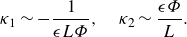
where the principal curvatures are given by
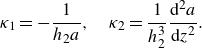 \begin{align} \kappa _1=-\frac {1}{h_2a}, \quad \kappa _2=\frac {1}{h_2^3}\frac {\mathrm{d}^2a }{\mathrm{d} {z^2}}. \end{align}
Last, making use of (2.8) and (2.10) we find from (2.24) that
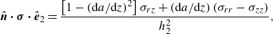 \begin{align} \hat {\boldsymbol{n}} \boldsymbol{\cdot } \boldsymbol{\sigma } \boldsymbol{\cdot } \hat {\boldsymbol{e}}_2 & = \frac {\left [1- \left({\mathrm{d} a}/{\mathrm{d} z} \right)^2\right]\sigma _{rz} + \left({\mathrm{d} a}/{\mathrm{d} z} \right)(\sigma _{rr}-\sigma _{zz})}{h_2^2}, \end{align}
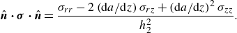 \begin{align} \hat {\boldsymbol{n}} \boldsymbol{\cdot } \boldsymbol{\sigma } \boldsymbol{\cdot } \hat {\boldsymbol{n}} & = \frac {\sigma _{rr}-2 \left({\mathrm{d} a}/{\mathrm{d} z} \right)\sigma _{rz} + \left({\mathrm{d} a}/{\mathrm{d} z} \right)^2\sigma _{zz}}{h_2^2}. \\[6pt] \nonumber \end{align}
2.6. Axial balance
Substituting expressions (2.30) and (2.33a ) into the meridional balance (2.26) yields
 \begin{equation} \frac {\left [1 - \left({\mathrm{d} a}/{\mathrm{d} z} \right)^2\right]\sigma _{rz} + \left({\mathrm{d} a}/{\mathrm{d} z} \right)(\sigma _{rr}-\sigma _{zz})}{h_2^2} +\frac {1}{h_2}\left (\frac {\mathrm{d} {\tau _2}}{\mathrm{d} {z}}+\frac {\mathrm{d} {a}}{\mathrm{d} {z}}\frac {\tau _2-\tau _1}{a}\right)=0. \end{equation}
Similarly, substituting (2.31) and (2.33b ) into the normal balance (2.27) yields
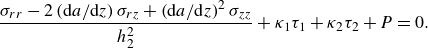 \begin{equation} \frac {\sigma _{rr}-2 \left({\mathrm{d} a}/{\mathrm{d} z} \right)\sigma _{rz} + \left({\mathrm{d} a}/{\mathrm{d} z} \right)^2\sigma _{zz}}{h_2^2}+\kappa _1\tau _1+\kappa _2\tau _2+P=0. \end{equation}
Note that (2.34)–(2.35) can be combined to get the axial stress balance
 \begin{equation} \frac {\mathrm{d}}{\mathrm{d} z}\left (T-\pi {a}^2 P\right)=2\pi {a}\left (\frac {\mathrm{d} {a}}{\mathrm{d} {z}}\sigma _{zz}-\sigma _{rz}\right), \end{equation}
where
 \begin{equation} T=\frac {2\pi a\tau _2}{h_2} \end{equation}
is the net axial elastic tension.
For a cusped shape we replace (2.13) by the requirement of zero axial tension at the ends of the capsule,
 \begin{equation} T(\pm L) =0. \end{equation}
This condition eliminates the possibility of point singularities at the tips, thus selecting the least-singular solution (Van Dyke Reference Van Dyke1964). Note that (2.38) is trivially satisfied for rounded ends, where $a\to 0$
and
$a\to 0$
and $|h_2|\to \infty$
(recall (2.7b
)).
$|h_2|\to \infty$
(recall (2.7b
)).
2.7. Elasticity
The evaluation of the Cauchy elastic tension $\mathcal{T}_s$
requires consideration of the elastic deformation. The principal values of
$\mathcal{T}_s$
requires consideration of the elastic deformation. The principal values of $\mathcal{T}_s$
,
$\mathcal{T}_s$
, $\tau _{1,2}$
, are functions of the principal extensional stretches (4.8). Dimensional arguments for the state of stretch imply that
$\tau _{1,2}$
, are functions of the principal extensional stretches (4.8). Dimensional arguments for the state of stretch imply that
 \begin{equation} \tau _{1,2}/G = \text{functions of }\lambda _1,\lambda _2,K/G. \end{equation}
Hereafter, we assume the Skalak model (Skalak et al. Reference Skalak, Tozeren, Zarda and Chien1973), where
 \begin{align} \frac {\tau _1}{G}=\frac {\lambda _1\left (\lambda _1^2-1\right)}{\lambda _2} + C\lambda _1\lambda _2\left (\lambda _1^2\lambda _2^2-1\right), \quad \frac {\tau _2}{G}=\frac {\lambda _2\left (\lambda _2^2-1\right)}{\lambda _1} + C\lambda _1\lambda _2\left (\lambda _1^2\lambda _2^2-1\right). \end{align}
The dimensionless parameter,
 \begin{equation} C=\frac {K/G-1}{2}, \end{equation}
is associated with resistance to area dilatation (Barthès-Biesel et al. Reference Barthès-Biesel, Diaz and Dhenin2002).
3. Strong flow: scaling
Henceforth, we focus upon the case of strong flow,
 \begin{equation} {Ca} \gg 1. \end{equation}
In this asymptotic limit, we expect $\epsilon$
to be small,
$\epsilon$
to be small,
 \begin{equation} \epsilon \ll 1. \end{equation}
Our interest is in the dependence of $\epsilon$
and
$\epsilon$
and $L/R$
upon
$L/R$
upon $Ca$
in the limit (3.1). It is preferable to temporarily adopt a mathematically equivalent approach where
$Ca$
in the limit (3.1). It is preferable to temporarily adopt a mathematically equivalent approach where $\epsilon$
and
$\epsilon$
and $L$
are considered as known, the former satisfying (3.2). The capillary number
$L$
are considered as known, the former satisfying (3.2). The capillary number $Ca$
and the reference radius
$Ca$
and the reference radius $R$
are then effectively considered as functions of
$R$
are then effectively considered as functions of $\epsilon$
and
$\epsilon$
and $L$
.
$L$
.
Prior to carrying an approximate scheme in the limit (3.2), we perform a scaling analysis. In what follows, we employ $\simeq$
to imply ‘of order’. In that context, the key estimates are
$\simeq$
to imply ‘of order’. In that context, the key estimates are
 \begin{align} z \simeq L, \quad a \simeq \epsilon L. \end{align}
It is evident from (2.5) and (3.3) that
 \begin{equation} R\simeq L \epsilon ^{2/3}. \end{equation}
We consider first the elastic stresses. Formulae (2.19) for the principal stretches in conjunction with (3.3) imply that $\lambda _1\simeq \epsilon L/R$
and
$\lambda _1\simeq \epsilon L/R$
and $\lambda _2\simeq L/R$
. Using (3.4) we find
$\lambda _2\simeq L/R$
. Using (3.4) we find
 \begin{align} \lambda _1 \simeq \epsilon ^{1/3}, \quad \lambda _2 \simeq \epsilon ^{-2/3} \end{align}
and, consequently, $\lambda _1\lambda _2\simeq \epsilon ^{-1/3}$
. Substitution into (2.40) gives
$\lambda _1\lambda _2\simeq \epsilon ^{-1/3}$
. Substitution into (2.40) gives
 \begin{align} \tau _1 \simeq G\epsilon ^{-1}, \quad \tau _2 \simeq G\epsilon ^{-7/3}, \end{align}
so that
 \begin{equation} \tau _2\gg \tau _1, \end{equation}
as would be expected under strong elongation.
It is evident from (2.32) that
 \begin{align} \kappa _1 \simeq \frac {1}{\epsilon L}, \quad \kappa _2 \simeq \frac {\epsilon }{L}, \end{align}
whereby
 \begin{align} \kappa _1 \tau _1\simeq GL^{-1}\epsilon ^{-2}, \quad \kappa _2 \tau _2\simeq GL^{-1}\epsilon ^{-4/3}, \end{align}
so, despite (3.7),
 \begin{equation} \kappa _1 \tau _1 \gg \kappa _2 \tau _2. \end{equation}
Consider now the divergence of $\mathcal{T}_s$
. It is evident from (2.30) and (3.7) that
$\mathcal{T}_s$
. It is evident from (2.30) and (3.7) that
 \begin{equation} \hat {\boldsymbol{e}}_2 \boldsymbol{\cdot } (\boldsymbol{\nabla }_s \boldsymbol{\cdot } \mathcal{T}_s) \simeq \tau _2/L. \end{equation}
It also follows from (2.31) and (3.10) that
 \begin{equation} \hat {\boldsymbol{n}} \boldsymbol{\cdot } (\boldsymbol{\nabla }_s \boldsymbol{\cdot } \mathcal{T}_s) \simeq \kappa _1 \tau _1. \end{equation}
Substituting (3.6) and (3.9a ) into (3.11) and (3.12) yields
 \begin{align} \hat {\boldsymbol{e}}_2 \boldsymbol{\cdot } (\boldsymbol{\nabla }_s \boldsymbol{\cdot } \mathcal{T}_s) \simeq GL^{-1}\epsilon ^{-7/3}, \quad \hat {\boldsymbol{n}} \boldsymbol{\cdot } (\boldsymbol{\nabla }_s \boldsymbol{\cdot } \mathcal{T}_s) \simeq GL^{-1}\epsilon ^{-2}. \end{align}
With the azimuthal component subdominant, the scaling relation between $Ca$
and
$Ca$
and $\epsilon$
is determined by the meridional balance (2.26). (In that sense, the present problem is fundamentally different from the classical problem of a deforming bubble.) To determine that relation we need to estimate the hydrodynamic stress. We first recall that
$\epsilon$
is determined by the meridional balance (2.26). (In that sense, the present problem is fundamentally different from the classical problem of a deforming bubble.) To determine that relation we need to estimate the hydrodynamic stress. We first recall that $\boldsymbol{\sigma }$
scales as
$\boldsymbol{\sigma }$
scales as $\mu E$
. For small
$\mu E$
. For small $\epsilon$
the shear-stress magnitude is amplified by
$\epsilon$
the shear-stress magnitude is amplified by $1 / \epsilon$
, so
$1 / \epsilon$
, so
 \begin{equation} \hat {\boldsymbol{n}}\boldsymbol{\cdot }\boldsymbol{\sigma }\boldsymbol{\cdot }\hat {\boldsymbol{e}}_2 \simeq \frac {\mu E}{\epsilon }. \end{equation}
Making use of (3.13a ) and (3.14), the meridional balance (2.26) gives
 \begin{equation} \frac {G}{L\epsilon ^{7/3}} \simeq \frac {\mu E}{\epsilon }. \end{equation}
Making use of (2.1) and (3.4) we obtain the requisite scaling
 \begin{equation} {Ca} \simeq \epsilon ^{-2/3}. \end{equation}
For future reference we note from (3.13) that the ratio of $\hat {\boldsymbol{n}} \boldsymbol{\cdot } (\boldsymbol{\nabla }_s \boldsymbol{\cdot } \mathcal{T}_s)$
to
$\hat {\boldsymbol{n}} \boldsymbol{\cdot } (\boldsymbol{\nabla }_s \boldsymbol{\cdot } \mathcal{T}_s)$
to $ \hat {\boldsymbol{e}}_2 \boldsymbol{\cdot } (\boldsymbol{\nabla }_s \boldsymbol{\cdot } \mathcal{T}_s)$
is
$ \hat {\boldsymbol{e}}_2 \boldsymbol{\cdot } (\boldsymbol{\nabla }_s \boldsymbol{\cdot } \mathcal{T}_s)$
is $\simeq \epsilon ^{1/3}$
.
$\simeq \epsilon ^{1/3}$
.
4. Analysis
We now go beyond scaling, carrying out a systematic approximation scheme. We retain our ‘inverted’ approach where $\epsilon$
and
$\epsilon$
and $L$
are considered as given.
$L$
are considered as given.
4.1. Dimensionless variables
At this stage we find it useful to introduce the dimensionless axial coordinate (recall (3.3a )),
 \begin{equation} \zeta = z / L. \end{equation}
This induces the definition of the dimensionless mapping $\varPsi (\zeta)$
,
$\varPsi (\zeta)$
,
 \begin{equation} Z(z) = \varPsi (\zeta), \end{equation}
and the dimensionless shape function $\varPhi (\zeta)$
(recall (3.3b
))
$\varPhi (\zeta)$
(recall (3.3b
))
 \begin{equation} a(z) = \epsilon L \varPhi (\zeta). \end{equation}
We note that $\varPhi (\zeta)$
is an even function while
$\varPhi (\zeta)$
is an even function while $\varPsi (\zeta)$
is an odd function.
$\varPsi (\zeta)$
is an odd function.
In dimensionless form, conditions (2.3) and (2.12) are
 \begin{align} \varPhi (\pm 1)=0, \quad \varPsi (\pm 1)=\pm 1, \end{align}
while the waist condition (2.4) becomes
 \begin{equation} \varPhi (0) = 1. \end{equation}
Following (3.4) we define
 \begin{equation}R= L \epsilon^{2/3} \chi,\end{equation}
The volume constraint (2.5) thus becomes
 \begin{equation} \int _{-1}^1\varPhi ^2(\zeta)\,\mathrm{d}\zeta =\frac {4\chi ^3}{3}. \end{equation}
The principal stretches (2.19) become, in terms of $\varPhi$
and
$\varPhi$
and $\varPsi$
,
$\varPsi$
,
 \begin{align} \lambda _1=\frac {\epsilon L }{R}\,\frac {\varPhi }{\sqrt {1-\varPsi ^2}}, \quad \lambda _2= \frac {L}{R}\,\frac {h_2\sqrt {1-\varPsi ^2}}{{\mathrm{d}\varPsi}/{\mathrm{d}\zeta}}. \end{align}
4.2. Approximations for elastic stresses
We proceed with a leading-order analysis. In what follows, the symbol ‘ $\sim$
’ implies ‘asymptotic to,’ with the understanding that the associated error is ‘algebraically small’ (i.e. asymptotically smaller than some positive power of
$\sim$
’ implies ‘asymptotic to,’ with the understanding that the associated error is ‘algebraically small’ (i.e. asymptotically smaller than some positive power of $\epsilon$
).
$\epsilon$
).
We begin with the geometric quantities. Using (4.1) and (4.3), we see that the scale factors introduced in (2.9) are given by
 \begin{align} h_1=\epsilon L \varPhi, \quad h_2\sim 1, \end{align}
while the principal curvatures (2.32) become
 \begin{align} \kappa _1\sim -\frac {1}{\epsilon L\varPhi }, \quad \kappa _2\sim \frac {\epsilon \varPhi }{L}. \end{align}
Upon making use of (4.6) and (4.9b ), the principal stretches (4.8) simplify to
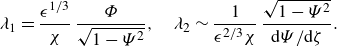 \begin{align} \lambda _1=\frac {\epsilon ^{1/3}}{\chi }\,\frac {\varPhi }{\sqrt {1-\varPsi ^2}}, \quad \lambda _2\sim \frac {1}{\epsilon ^{2/3}\chi }\,\frac {\sqrt {1-\varPsi ^2}}{{\mathrm{d}\varPsi}/{\mathrm{d}\zeta}}. \end{align}
Consider now the elastic constitutive relations (2.40). Making use of (3.5), we find that they are approximated by
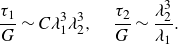 \begin{align} \frac {\tau _1}{G}\sim C\lambda _1^3\lambda _2^3, \quad \frac {\tau _2}{G}\sim \frac {\lambda _2^3}{\lambda _1}. \end{align}
Substituting (4.11) thus gives
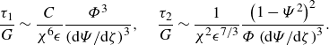 \begin{align} \frac {\tau _1}{G}\sim \frac {C}{\chi ^6\epsilon }\frac {\varPhi ^3}{\left({\mathrm{d}\varPsi}/{\mathrm{d}\zeta} \right)^3}, \quad \frac {\tau _2}{G}\sim \frac {1}{\chi ^2\epsilon ^{7/3}}\frac {\left (1-\varPsi ^2\right)^2}{\varPhi \left({\mathrm{d}\varPsi}/{\mathrm{d}\zeta} \right)^3}. \end{align}
Consider now the divergence of $\mathcal{T}_s$
. Making use of (2.30) and noting that
$\mathcal{T}_s$
. Making use of (2.30) and noting that $\tau _2\gg \tau _1$
we obtain the meridional component
$\tau _2\gg \tau _1$
we obtain the meridional component
 \begin{equation} \hat {\boldsymbol{e}}_2 \boldsymbol{\cdot } (\boldsymbol{\nabla }_s \boldsymbol{\cdot } \mathcal{T}_s) \sim \frac {1}{a} \frac {\mathrm{d} }{\mathrm{d} {z}}(a \tau _2). \end{equation}
Upon substituting (4.1)–(4.3) and (4.13b ) we obtain
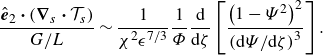 \begin{equation} \frac {\hat {\boldsymbol{e}}_2 \boldsymbol{\cdot } (\boldsymbol{\nabla }_s \boldsymbol{\cdot } \mathcal{T}_s)}{{G}/{L}} \sim \frac {1}{\chi ^2\epsilon ^{7/3}} \frac {1}{\varPhi } \frac {\mathrm{d} }{\mathrm{d} {\zeta }}\left [\frac {\left (1-\varPsi ^2\right)^2}{\left({\mathrm{d}\varPsi}/{\mathrm{d}\zeta}\right)^3}\right]. \end{equation}
Making use of (2.31) and (3.10) we obtain $\hat {\boldsymbol{n}} \boldsymbol{\cdot } (\boldsymbol{\nabla }_s \boldsymbol{\cdot } \mathcal{T}_s) \sim \kappa _1 \tau _1$
. Substitution of (4.10a
) and (4.13a
) gives
$\hat {\boldsymbol{n}} \boldsymbol{\cdot } (\boldsymbol{\nabla }_s \boldsymbol{\cdot } \mathcal{T}_s) \sim \kappa _1 \tau _1$
. Substitution of (4.10a
) and (4.13a
) gives
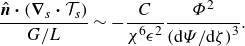 \begin{equation} \frac {\hat {\boldsymbol{n}} \boldsymbol{\cdot } (\boldsymbol{\nabla }_s \boldsymbol{\cdot } \mathcal{T}_s)}{{G}/{L}} \sim -\frac {C}{\chi ^6\epsilon ^2} \frac {\varPhi ^2}{\left({\mathrm{d}\varPsi}/{\mathrm{d}\zeta}\right)^3}. \end{equation}
The negative sign implies a surface-tension-like ‘inward’ contribution to the normal force balance.
4.3. Flow
In the limit (3.2), the flow coincides with that about a slender rigid body (Batchelor Reference Batchelor1970; Cox Reference Cox1970; Tillett Reference Tillett1970). In analysing flows about rigid bodies, interest typically lies in the hydrodynamic force acting on the body (or, by extension, in the hydrodynamic couple or the net stresslet strength). For these quantities, it suffices to determine the distribution of Stokeslets that represent the body.
In the present problem, however, we need the actual shear stress at the boundary of the body. For that reason, it is desirable to employ an analysis in the spirit of matched asymptotic expansions, where the Stokeslet distribution represents an approximation on the ‘long’ scale of body length which is supplemented by a comparable approximation on the ‘short’ cross-sectional scale $\epsilon$
.
$\epsilon$
.
Given our desire for an algebraically accurate approximation, we prefer to employ the analysis of Keller & Rubinow (Reference Keller and Rubinow1976), which for the most part avoids an expansion in inverse powers of $\ln \epsilon$
. Adapting their analysis to the present notation, the long-scale flow is written as a superposition of the ambient flow (2.22) and a collection of Stokeslets (of strength
$\ln \epsilon$
. Adapting their analysis to the present notation, the long-scale flow is written as a superposition of the ambient flow (2.22) and a collection of Stokeslets (of strength $\mu E L \mathcal F$
per unit length) along the symmetry axis,
$\mu E L \mathcal F$
per unit length) along the symmetry axis,
 \begin{equation} \frac {\boldsymbol{u}}{EL}\sim \zeta \hat {\boldsymbol{e}}_z-\frac {\rho }{2}\hat {\boldsymbol{e}}_{r} + \frac {1}{8\pi }\def\negativespace{} \int _{-1}^1 \def\negativespace{}\mathcal F(\xi)\def\negativespace{} \left \{ \frac {\hat {\boldsymbol{e}}_z}{\left [\rho ^2 + (\zeta -\xi)^2\right]^{1/2}} + (\zeta -\xi) \frac {\hat {\boldsymbol{e}}_r \rho + \hat {\boldsymbol{e}}_z(\zeta -\xi)}{\left [\rho ^2 + (\zeta -\xi)^2\right]^{3/2}}\def\negativespace{}\right \} \mathrm{d}\xi, \end{equation}
wherein (cf. (4.1))
 \begin{equation} \rho =r/L. \end{equation}
On the cross-sectional scale, where $\rho =O(\epsilon)$
, the flow is primarily in the axial direction. Thus, making use of the form (2.23),
$\rho =O(\epsilon)$
, the flow is primarily in the axial direction. Thus, making use of the form (2.23), ${w}/{EL}=O(1)$
while
${w}/{EL}=O(1)$
while $u/EL$
is
$u/EL$
is $O(\epsilon)$
. In particular, imposing the no slip condition at
$O(\epsilon)$
. In particular, imposing the no slip condition at $\rho / \epsilon =\varPhi$
and compatibility with (4.17) yields (see equations (1), (2) and (9) in Keller & Rubinow (Reference Keller and Rubinow1976))
$\rho / \epsilon =\varPhi$
and compatibility with (4.17) yields (see equations (1), (2) and (9) in Keller & Rubinow (Reference Keller and Rubinow1976))
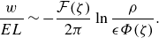 \begin{equation} \frac {w}{EL} \sim -\frac {\mathcal F(\zeta)}{2\pi }\ln \frac {\rho }{\epsilon \varPhi (\zeta)}. \end{equation}
The integral equation governing the Stokelet distribution $\mathcal F(\zeta)$
was determined by Keller & Rubinow (Reference Keller and Rubinow1976) via matching between the long-scale and short-scale solutions (see equation (12) in Keller & Rubinow (Reference Keller and Rubinow1976)). Adapting to the present notation, this equation reads
$\mathcal F(\zeta)$
was determined by Keller & Rubinow (Reference Keller and Rubinow1976) via matching between the long-scale and short-scale solutions (see equation (12) in Keller & Rubinow (Reference Keller and Rubinow1976)). Adapting to the present notation, this equation reads
 \begin{equation} 4\pi \zeta + [\ln (1-\zeta ^2)-1] \mathcal F(\zeta) + \int _{-1}^1 \frac {\mathcal F(\xi)-\mathcal F(\zeta)}{|\xi -\zeta |}\,\mathrm{d}\xi = 2\mathcal F(\zeta) \ln \frac {\epsilon \varPhi (\zeta)}{2}. \end{equation}
Consistently with our approach (and, more generally, with established asymptotic practices (Fraenkel Reference Fraenkel1969)), we retain terms that are logarithmically small in $\epsilon$
while neglecting algebraically small corrections.
$\epsilon$
while neglecting algebraically small corrections.
We can now calculate the hydrodynamic shear stress in terms of $\mathcal F$
. It is evident that on the cross-sectional scale
$\mathcal F$
. It is evident that on the cross-sectional scale $\sigma _{rz} \sim \mu \,\partial {w}/\partial {r}$
. Substituting (4.18) and (4.19) we obtain the
$\sigma _{rz} \sim \mu \,\partial {w}/\partial {r}$
. Substituting (4.18) and (4.19) we obtain the $O(\epsilon ^{-1})$
stress (cf. (3.14)),
$O(\epsilon ^{-1})$
stress (cf. (3.14)),
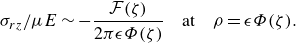 \begin{equation} \sigma _{rz}/\mu E \sim -\frac {\mathcal F(\zeta)}{2\pi \epsilon \varPhi (\zeta)} \quad \text{at} \quad \rho = \epsilon \varPhi (\zeta). \end{equation}
It is readily verified that both $\sigma _{rr}/\mu E$
and
$\sigma _{rr}/\mu E$
and $\sigma _{zz}/\mu E$
are
$\sigma _{zz}/\mu E$
are $O(1)$
on the cross-sectional scale. From (2.33) we then conclude that
$O(1)$
on the cross-sectional scale. From (2.33) we then conclude that
 \begin{align} \frac {\hat {\boldsymbol{n}} \boldsymbol{\cdot } \boldsymbol{\sigma } \boldsymbol{\cdot } \hat {\boldsymbol{e}}_2}{\mu E} \sim -\frac {\mathcal F(\zeta)}{2\pi \epsilon \varPhi (\zeta)}, \quad \frac {\hat {\boldsymbol{n}} \boldsymbol{\cdot } \boldsymbol{\sigma } \boldsymbol{\cdot } \hat {\boldsymbol{n}}}{\mu E} = O(1). \end{align}
4.4. Dominant balances
Requiring that the two terms in meridional equilibrium (2.26) balance, we find using (4.15) and (4.22a ) that
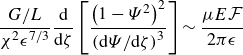 \begin{equation}\frac{G/L}{\chi^2\epsilon^{7/3}} \frac{\text{d}}{\text{d}\zeta}\left[\frac{\left(1-\varPsi^2\right)^2}{\left({\text{d}\varPsi}/{\text{d}\zeta} \right)^3}\right]\sim \frac{\mu E\mathcal F}{2\pi\epsilon}\end{equation}
Making use of (2.1) and (4.6) we obtain
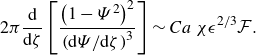 \begin{equation} 2\pi \frac {\mathrm{d} }{\mathrm{d} {\zeta }}\left [\frac {\left (1-\varPsi ^2\right)^2}{ \left({\mathrm{d}\varPsi}/{\mathrm{d}\zeta} \right)^3}\right] \sim {Ca} \, \chi \epsilon ^{2/3} \mathcal F. \end{equation}
Thus, $Ca$
scales as
$Ca$
scales as $\epsilon ^{-2/3}$
, as already anticipated in (3.16). Defining the rescaled capillary number
$\epsilon ^{-2/3}$
, as already anticipated in (3.16). Defining the rescaled capillary number
 \begin{equation} \widetilde {Ca} = {Ca} \, \chi \epsilon ^{2/3} \end{equation}
we obtain
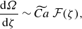 \begin{equation} \frac {\mathrm{d} {\varOmega }}{\mathrm{d} {\zeta }} \sim \widetilde {Ca} \, \mathcal F(\zeta), \end{equation}
wherein
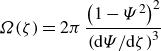 \begin{equation} \varOmega (\zeta)=2\pi \,\frac {\left (1-\varPsi ^2\right)^2}{ \left({\mathrm{d}\varPsi}/{\mathrm{d}\zeta} \right)^3} \end{equation}
is a (leading-order) dimensionless version of the axial tension (2.37),
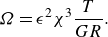 \begin{equation} \varOmega = \epsilon ^2\chi ^3 \frac {T}{GR}. \end{equation}
Consider now the normal balance (2.27). It follows from (2.1), (4.6), (4.16) and (4.22b
) that the ratio of $\hat {\boldsymbol{n}} \boldsymbol{\cdot } \boldsymbol{\sigma } \boldsymbol{\cdot } \hat {\boldsymbol{n}}$
to
$\hat {\boldsymbol{n}} \boldsymbol{\cdot } \boldsymbol{\sigma } \boldsymbol{\cdot } \hat {\boldsymbol{n}}$
to $\hat {\boldsymbol{n}} \boldsymbol{\cdot } (\boldsymbol{\nabla }_s \boldsymbol{\cdot } \mathcal{T}_s)$
is of order
$\hat {\boldsymbol{n}} \boldsymbol{\cdot } (\boldsymbol{\nabla }_s \boldsymbol{\cdot } \mathcal{T}_s)$
is of order ${Ca}\,\epsilon ^{4/3}$
, or, using (3.16), of order
${Ca}\,\epsilon ^{4/3}$
, or, using (3.16), of order $\epsilon ^{2/3}$
. This was to be expected, we already saw from the scaling estimate (3.13) that the normal component of
$\epsilon ^{2/3}$
. This was to be expected, we already saw from the scaling estimate (3.13) that the normal component of $\boldsymbol{\nabla }_s \boldsymbol{\cdot } \mathcal{T}_s$
is
$\boldsymbol{\nabla }_s \boldsymbol{\cdot } \mathcal{T}_s$
is $O(\epsilon ^{1/3})$
relative to meridional component. The hydrodynamic considerations, on the other hand, have revealed that the ratio of the normal Newtonian stress to the shear Newtonian stress is of order
$O(\epsilon ^{1/3})$
relative to meridional component. The hydrodynamic considerations, on the other hand, have revealed that the ratio of the normal Newtonian stress to the shear Newtonian stress is of order $\epsilon$
. It follows that the hydrodynamic traction does not participate at the dominant balance of (2.27), which must therefore involve the elastic force (4.16) and the core pressure. Defining the dimensionless pressure
$\epsilon$
. It follows that the hydrodynamic traction does not participate at the dominant balance of (2.27), which must therefore involve the elastic force (4.16) and the core pressure. Defining the dimensionless pressure
 \begin{equation} \varPi = \frac {P}{\mu E}, \end{equation}
we therefore obtain
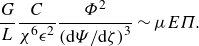 \begin{equation} \frac {G}{L}\frac {C}{\chi ^6\epsilon ^2} \frac {\varPhi ^2}{\left({\mathrm{d}\varPsi}/{\mathrm{d}\zeta} \right)^3}\sim \mu E \varPi. \end{equation}
Making use of (2.1), (4.6) and (4.25) yields the dimensionless balance
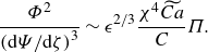 \begin{equation} \frac {\varPhi ^2}{\left({\mathrm{d}\varPsi}/{\mathrm{d}\zeta}\right)^3} \sim \epsilon ^{2/3} \frac {\chi ^4 \widetilde {Ca}}{C} \varPi. \end{equation}
It follows that $\varPi$
scales as
$\varPi$
scales as $\epsilon ^{-2/3}$
– namely as the capillary number. Defining the rescaled pressure,
$\epsilon ^{-2/3}$
– namely as the capillary number. Defining the rescaled pressure,
 \begin{equation} \widetilde \varPi = \epsilon ^{2/3} \frac {\chi ^4 \widetilde {Ca}}{C} \varPi, \end{equation}
we find that (4.31) is simplified to
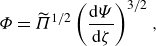 \begin{equation} \varPhi = {\widetilde \varPi }^{1/2} \left (\frac {\mathrm{d} {\varPsi }}{\mathrm{d} {\zeta }}\right)^{ \def\negativespace{} 3/2}, \end{equation}
where we used the fact that both $\varPhi$
and
$\varPhi$
and $\mathrm{d}\varPsi /\mathrm{d}\zeta$
are non-negative.
$\mathrm{d}\varPsi /\mathrm{d}\zeta$
are non-negative.
5. Reduced problem
We now summarise the reduced problem governing the mapping $\varPsi$
and the tension
$\varPsi$
and the tension $\varOmega$
introduced in (4.27). Relation (4.27) is rewritten as a first-order differential equation,
$\varOmega$
introduced in (4.27). Relation (4.27) is rewritten as a first-order differential equation,
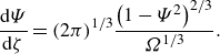 \begin{equation} \frac {\mathrm{d} {\varPsi }}{\mathrm{d} {\zeta }}=(2\pi)^{1/3}\frac {\left (1-\varPsi ^2\right)^{2/3}}{\varOmega ^{1/3}}. \end{equation}
The shape is obtained from (4.33) and (5.1)
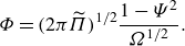 \begin{equation} \varPhi = (2\pi \widetilde \varPi)^{1/2}\frac {1-\varPsi ^2}{\varOmega ^{1/2}}. \end{equation}
Substituting (4.26) and (5.2) into (4.20), we obtain
 \begin{equation} 4\pi \widetilde {Ca}\,\zeta + \left [\ln (1-\zeta ^2)-1\right] \varOmega ^{\prime}(\zeta) + \int _{-1}^1 \frac {\varOmega ^{\prime}(\xi)-\varOmega ^{\prime}(\zeta)}{|\xi -\zeta |}\,\mathrm{d}\xi = \varOmega ^{\prime}(\zeta) \ln \frac {\epsilon ^2 \pi \widetilde \varPi (1-\varPsi ^{2})}{2\varOmega }, \end{equation}
where the prime denotes differentiation. The deformation problem is therefore governed by the set (5.1) and (5.3).
Since $\varPsi (\zeta)$
is an odd function,
$\varPsi (\zeta)$
is an odd function, $\varOmega (\zeta)$
must be even: see (4.27). We therefore solve only for
$\varOmega (\zeta)$
must be even: see (4.27). We therefore solve only for $\zeta \gt 0$
, replacing (5.3) by
$\zeta \gt 0$
, replacing (5.3) by
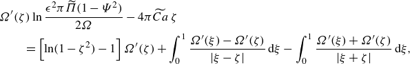 \begin{align} &\varOmega ^{\prime}(\zeta) \ln \frac {\epsilon ^2 \pi \widetilde \varPi (1-\varPsi ^{2})}{2\varOmega } - 4\pi \widetilde {Ca}\,\zeta \nonumber \\ &\qquad = \left [\ln (1-\zeta ^2)-1\right] \varOmega ^{\prime}(\zeta) + \int _0^1 \frac {\varOmega ^{\prime}(\xi)-\varOmega ^{\prime}(\zeta)}{|\xi -\zeta |}\,\mathrm{d}\xi - \int _0^1 \frac {\varOmega ^{\prime}(\xi) + \varOmega ^{\prime}(\zeta)}{|\xi + \zeta |}\,\mathrm{d}\xi, \end{align}
and adding the symmetry conditions
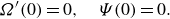 \begin{align} \varOmega ^{\prime}(0) = 0, \quad \varPsi (0) =0. \end{align}
These are supplemented by the end condition,
 \begin{equation} \varPsi ( 1)=1, \end{equation}
which follows from (4.4) and (5.2); the waist condition
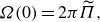 \begin{equation} \varOmega (0)=2\pi {\widetilde \varPi }, \end{equation}
which follows from (4.5) and (5.2); and the tip condition,
 \begin{equation} \varOmega (1)=0, \end{equation}
which constitutes the dimensionless version of (2.38).
We note that (5.5a
) is trivially satisfied by (5.4). Thus, (5.1) and (5.4) together with the four conditions (5.5b
)–(5.8) presumably provide a closed system for $\varOmega (\zeta)$
and
$\varOmega (\zeta)$
and $\varPsi (\zeta)$
, in which the dimensionless parameters
$\varPsi (\zeta)$
, in which the dimensionless parameters $\widetilde {Ca}$
and
$\widetilde {Ca}$
and $\widetilde \varPi$
are determined as part of the solution. Conveniently, the above problem is independent of
$\widetilde \varPi$
are determined as part of the solution. Conveniently, the above problem is independent of $\chi$
. Once the problem is solved,
$\chi$
. Once the problem is solved, $\chi$
may be determined from the relation
$\chi$
may be determined from the relation
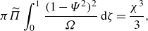 \begin{equation} \pi \widetilde \varPi \int _0^1 \frac {(1-\varPsi ^2)^2}{\varOmega }\,\mathrm{d}\zeta = \frac {\chi ^3}{3}, \end{equation}
which follows from (4.7) in conjunction with (5.2). The dimensionless capsule length and capillary number corresponding to the chosen value of $\epsilon$
are then recovered from (4.6) and (4.25), respectively.
$\epsilon$
are then recovered from (4.6) and (4.25), respectively.
We note that the reduced problem is independent of $C$
. Once the problem is solved and
$C$
. Once the problem is solved and $\widetilde \varPi$
is calculated, the value of
$\widetilde \varPi$
is calculated, the value of $C$
affects the core pressure
$C$
affects the core pressure $\varPi$
, see (4.32). Otherwise,
$\varPi$
, see (4.32). Otherwise, $C$
does not affect the capsule shape at the present leading-order approximation scheme.
$C$
does not affect the capsule shape at the present leading-order approximation scheme.
6. Logarithmic approximation
Let us derive a ‘logarithmically accurate’ approximation by considering $\ln (2/\epsilon ^2)$
as being asymptotically large. The associated leading-order balance in (5.4) then takes place between the two terms on the left-hand side. We can therefore make the leading-order approximation
$\ln (2/\epsilon ^2)$
as being asymptotically large. The associated leading-order balance in (5.4) then takes place between the two terms on the left-hand side. We can therefore make the leading-order approximation
 \begin{equation} \frac {\mathrm{d} {\varOmega }}{\mathrm{d} {\zeta }}\approx -\frac {4\pi \widetilde {Ca}\,\zeta }{\ln \left ({2}/{\epsilon^2}\right)}, \end{equation}
where the symbol ‘ $\approx$
’ is used to represent the ‘logarithmic’ approximation.
$\approx$
’ is used to represent the ‘logarithmic’ approximation.
We can immediately integrate (6.1) and apply the tip condition (5.8) to get the leading-order tension
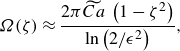 \begin{equation} \varOmega (\zeta)\approx \frac {2\pi \widetilde {Ca}\, \left (1-\zeta ^2\right)}{\ln \left ({2}/{\epsilon ^2}\right)}, \end{equation}
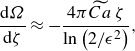
whereby condition (5.7) yields
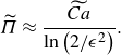 \begin{equation} \widetilde \varPi \approx \frac {\widetilde {Ca}}{\ln \left ({2}/{\epsilon ^2}\right)}. \end{equation}
From (5.1) we then obtain the separable equation
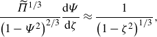 \begin{equation} \frac {{\widetilde \varPi }^{1/3}}{\left (1-\varPsi ^2\right)^{2/3}} \frac {\mathrm{d} {\varPsi }}{\mathrm{d} {\zeta }}\approx \frac {1}{\left (1-\zeta ^2\right)^{1/3}}, \end{equation}
which may be immediately integrated to give
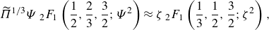 \begin{equation} {\widetilde \varPi }^{1/3}\varPsi \,{}_2F_1\left (\frac {1}{2},\frac {2}{3},\frac {3}{2};\varPsi ^2\right)\approx \zeta \,{}_2F_1\left (\frac {1}{3},\frac {1}{2},\frac {3}{2};\zeta ^2\right), \end{equation}
in which ${}_2F_1$
is a hypergeometric function, and the integration constant vanishes because of condition (5.5b
).
${}_2F_1$
is a hypergeometric function, and the integration constant vanishes because of condition (5.5b
).
Application of (5.6) gives
 \begin{equation} \widetilde \varPi \approx {\left [\frac {_2F_1\left ({1}/{3}, {1}/{2}, {3}/{2};1\right)}{_2F_1\left ({1}/{2}, {2}/{3}, {3}/{2};1\right)}\right]}^3 = \frac {\pi ^{3/2} \left[\Gamma \left({5}/{6} \right) \right]^3}{54 \left[\Gamma \left({7}/{6} \right) \right]^6}. \end{equation}
By expanding (6.5) near $\zeta =1$
and
$\zeta =1$
and $\varPsi =1$
we obtain, using (6.6),
$\varPsi =1$
we obtain, using (6.6),
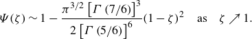 \begin{equation} \varPsi (\zeta) \sim 1 - \frac {\pi ^{3/2} \left[\Gamma \left({7}/{6} \right) \right]^3}{2 \left[\Gamma \left({5}/{6} \right)\right]^6}(1-\zeta)^2 \quad \text{as} \quad \zeta \nearrow 1. \end{equation}
Given (6.6), the implicit relation (6.5) provides $\varPsi$
as a function of
$\varPsi$
as a function of $\zeta$
, independent of
$\zeta$
, independent of $\epsilon$
. Substituting (6.2) and (6.3) into (5.2) yields the shape
$\epsilon$
. Substituting (6.2) and (6.3) into (5.2) yields the shape
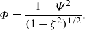 \begin{equation} \varPhi = \frac {1-\varPsi ^2}{(1-\zeta ^2)^{1/2}}. \end{equation}
Note that (6.7) and (6.8) implies that $\varPhi$
behaves like
$\varPhi$
behaves like $(1-\zeta)^{3/2}$
as
$(1-\zeta)^{3/2}$
as $\zeta \nearrow 1$
, consistently with the assumption of a cusp. The universal shape, as obtained from substitution of (6.5) and (6.6) into (6.8), is shown in figure 2(a).
$\zeta \nearrow 1$
, consistently with the assumption of a cusp. The universal shape, as obtained from substitution of (6.5) and (6.6) into (6.8), is shown in figure 2(a).
Logarithmic approximation: (a) universal shape, $\varPhi$
versus
$\varPhi$
versus $\zeta$
; (b) physical shape in the
$\zeta$
; (b) physical shape in the $(r/R,z/R)$
coordinates for
$(r/R,z/R)$
coordinates for ${Ca}=5$
.
${Ca}=5$
.
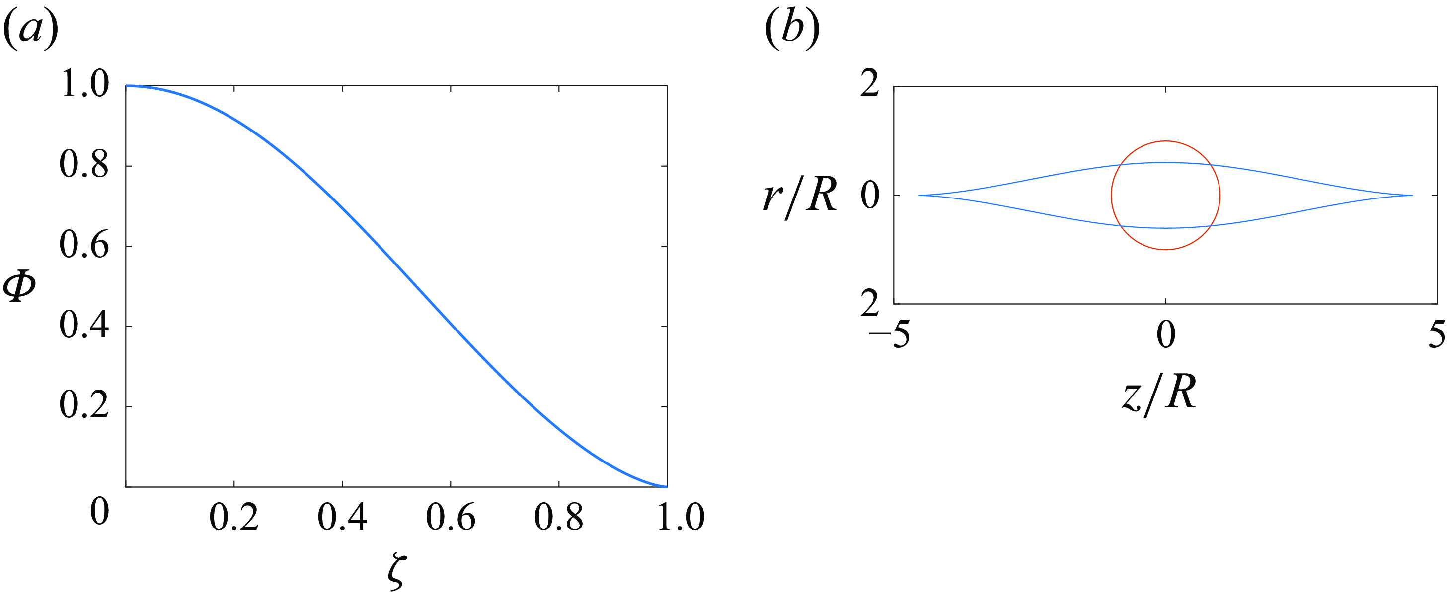
The volume constraint (5.9) reads here
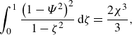 \begin{equation} \int _0^1 \frac {\left (1-\varPsi ^2\right) ^2}{1-\zeta ^2}\,\mathrm{d}\zeta = \frac {2\chi ^3}{3}, \end{equation}
independently of $\epsilon$
. Evaluation using the universal function provided by (6.5) and (6.6) yields
$\epsilon$
. Evaluation using the universal function provided by (6.5) and (6.6) yields
 \begin{equation} \chi =0.8448\ldots. \end{equation}
The capsule length is obtained from (4.6) as
 \begin{equation} L/R \approx 1.1837 \epsilon ^{-2/3}, \end{equation}
while evaluation of (6.6) gives
 \begin{equation} \widetilde \varPi =0.2326\ldots. \end{equation}
The capillary number is obtained from (4.25), which upon using (6.3), (6.10) and (6.12) gives
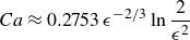 \begin{equation} {Ca} \approx 0.2753\,\epsilon ^{-2/3}\ln \dfrac{2}{\epsilon ^2}\end{equation}
With the universal shape $\varPhi (\zeta)$
available, we may employ (4.1), (4.3) and (6.11) to plot the ‘physical shape’ of the capsule on the length scale
$\varPhi (\zeta)$
available, we may employ (4.1), (4.3) and (6.11) to plot the ‘physical shape’ of the capsule on the length scale $R$
for a given capillary number, with the slenderness
$R$
for a given capillary number, with the slenderness $\epsilon$
determined from (6.13). In figure 2(b) we plot that physical shape for
$\epsilon$
determined from (6.13). In figure 2(b) we plot that physical shape for ${Ca}=5$
. The reference spherical shape is also shown.
${Ca}=5$
. The reference spherical shape is also shown.
Normalised capsule length $L/R$
as a function of
$L/R$
as a function of $Ca$
: solid, logarithmic approximation, (6.11) and (6.13); squares, data set from Dodson III & Dimitrakopoulos (Reference Dodson and Dimitrakopoulos2009); diamonds, data set from Dupont & Barthés-Biesel (Reference Dupont and Barthés-Biesel2024).
$Ca$
: solid, logarithmic approximation, (6.11) and (6.13); squares, data set from Dodson III & Dimitrakopoulos (Reference Dodson and Dimitrakopoulos2009); diamonds, data set from Dupont & Barthés-Biesel (Reference Dupont and Barthés-Biesel2024).
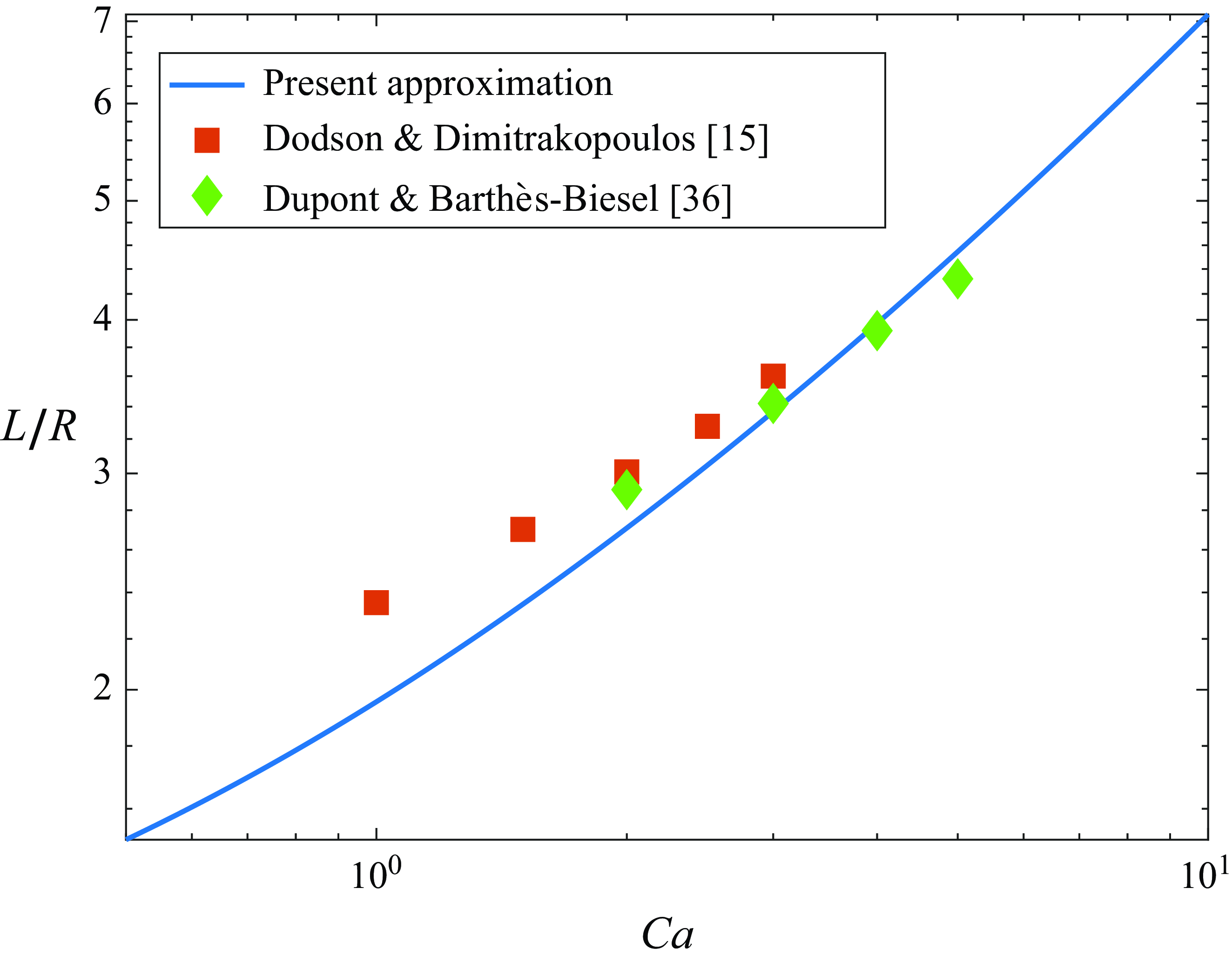
In comparing our approximation with the existing literature we employ two sets of data points, both obtained for the Skalak law (2.40) with $C=1$
. The first is obtained from the numerical simulations of Dodson III & Dimitrakopoulos (Reference Dodson and Dimitrakopoulos2009). While these authors consider planar hyperbolic flow, it is plausible that these results are quantitatively similar to those of uniaxial flow; indeed, Hinch & Acrivos (Reference Hinch and Acrivos1979) analysed bubble deformation in planar flow by viewing it as a perturbation of the axisymmetric case. By interpolating from figure 16 in Dodson III & Dimitrakopoulos (Reference Dodson and Dimitrakopoulos2009), we obtained values of
$C=1$
. The first is obtained from the numerical simulations of Dodson III & Dimitrakopoulos (Reference Dodson and Dimitrakopoulos2009). While these authors consider planar hyperbolic flow, it is plausible that these results are quantitatively similar to those of uniaxial flow; indeed, Hinch & Acrivos (Reference Hinch and Acrivos1979) analysed bubble deformation in planar flow by viewing it as a perturbation of the axisymmetric case. By interpolating from figure 16 in Dodson III & Dimitrakopoulos (Reference Dodson and Dimitrakopoulos2009), we obtained values of $L/R$
for the
$L/R$
for the $Ca$
values 1, 1.5, 2 and 2.5; in addition, Dodson III & Dimitrakopoulos (Reference Dodson and Dimitrakopoulos2009) cite the value
$Ca$
values 1, 1.5, 2 and 2.5; in addition, Dodson III & Dimitrakopoulos (Reference Dodson and Dimitrakopoulos2009) cite the value $L/R=3.6$
for
$L/R=3.6$
for ${Ca}=3$
. The second set was kindly provided by Dupont & Barthés-Biesel (Reference Dupont and Barthés-Biesel2024) who recently performed numerical simulations of the present problem. We used their results for the
${Ca}=3$
. The second set was kindly provided by Dupont & Barthés-Biesel (Reference Dupont and Barthés-Biesel2024) who recently performed numerical simulations of the present problem. We used their results for the $Ca$
values 2, 3, 4 and 5. Note that the physical shape in figure 2(b) has been portrayed for their maximal value of
$Ca$
values 2, 3, 4 and 5. Note that the physical shape in figure 2(b) has been portrayed for their maximal value of $Ca$
.
$Ca$
.
The comparison is shown in figure 3 where the theoretical approximation for $L/R$
as a function of
$L/R$
as a function of $Ca$
is obtained from (6.11) and (6.13). Given the crude nature of the logarithmic approximation and the rather modest
$Ca$
is obtained from (6.11) and (6.13). Given the crude nature of the logarithmic approximation and the rather modest $Ca$
-values which have been employed in the simulations, the agreement is gratifying.
$Ca$
-values which have been employed in the simulations, the agreement is gratifying.
7. Neo-Hookean membranes
The preceding analysis was carried out for an elastic membrane governed by the Skalak constitutive description. In principle, it can be carried out for other elastic models, provided the membrane reaches a steady state under large deformation.
In fact, the very possibility of steady state can be inferred from a scaling analysis akin to that carried out in § 3. As an illustration, consider the neo-Hookean model (Barthès-Biesel et al. Reference Barthès-Biesel, Diaz and Dhenin2002) where (2.40) is replaced by
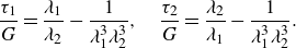 \begin{align} \frac {\tau _1}{G}=\frac {\lambda _1}{\lambda _2} - \frac {1}{\lambda _1^3\lambda _2^3}, \quad \frac {\tau _2}{G}=\frac {\lambda _2}{\lambda _1} - \frac {1}{\lambda _1^3\lambda _2^3}. \end{align}
Making use of (3.5), we find that the stress estimates (3.6) are replaced by
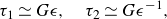 \begin{align} \tau _1 \simeq G\epsilon, \quad \tau _2 \simeq G\epsilon ^{-1}, \end{align}
while the estimates (3.9) are replaced by
 \begin{equation} \kappa _1 \tau _1,\kappa _2 \tau _2\simeq GL^{-1}. \end{equation}
Since (3.11) still holds, we find using (7.2 b) that (3.13 a) is replaced by
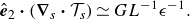 \begin{equation} \hat {\boldsymbol{e}}_2 \boldsymbol{\cdot } (\boldsymbol{\nabla }_s \boldsymbol{\cdot } \mathcal{T}_s) \simeq GL^{-1}\epsilon ^{-1}. \end{equation}
Also, from (2.31) and (7.3) it follows that (3.13 b) is replaced by
 \begin{equation} \hat {\boldsymbol{n}} \boldsymbol{\cdot } (\boldsymbol{\nabla }_s \boldsymbol{\cdot } \mathcal{T}_s) \simeq GL^{-1}. \end{equation}
Thus, just like in the Skalak model, $\hat {\boldsymbol{e}}_2 \boldsymbol{\cdot } (\boldsymbol{\nabla }_s \boldsymbol{\cdot } \mathcal{T}_s) \gg \hat {\boldsymbol{n}} \boldsymbol{\cdot } (\boldsymbol{\nabla }_s \boldsymbol{\cdot } \mathcal{T}_s)$
. Balancing (7.4) with (3.14), the meridional balance (2.26) gives (cf. (3.15))
$\hat {\boldsymbol{e}}_2 \boldsymbol{\cdot } (\boldsymbol{\nabla }_s \boldsymbol{\cdot } \mathcal{T}_s) \gg \hat {\boldsymbol{n}} \boldsymbol{\cdot } (\boldsymbol{\nabla }_s \boldsymbol{\cdot } \mathcal{T}_s)$
. Balancing (7.4) with (3.14), the meridional balance (2.26) gives (cf. (3.15))
 \begin{equation} \frac {G}{L\epsilon } \simeq \frac {\mu E}{\epsilon }.\end{equation}
Making use of (2.1) and (3.4) we obtain the scaling
 \begin{equation} {Ca} \simeq \epsilon ^{2/3}, \end{equation}
which contradicts (3.2). This indicates the impossibility of a steady slender shape. Our conclusion is compatible with the numerical simulations of Barthès-Biesel et al. (Reference Barthès-Biesel, Diaz and Dhenin2002), who observed that a neo-Hookean capsule stretches indefinitely in an elongational flow.
The key to a possible slender limit is the need for the elastic stresses to increase sufficiently fast with diminishing $\epsilon$
so as to overcome the viscous stress that grows as
$\epsilon$
so as to overcome the viscous stress that grows as $\epsilon ^{-1}$
, see (3.14). For a given reference radius
$\epsilon ^{-1}$
, see (3.14). For a given reference radius $R$
, the meridional components of
$R$
, the meridional components of $\boldsymbol{\nabla }_s \boldsymbol{\cdot } \mathcal{T}_s$
increases with diminishing
$\boldsymbol{\nabla }_s \boldsymbol{\cdot } \mathcal{T}_s$
increases with diminishing $\epsilon$
in both the Skalak and neo-Hookean models, but at quite different rates. In the Skalak model, it scales as
$\epsilon$
in both the Skalak and neo-Hookean models, but at quite different rates. In the Skalak model, it scales as $\epsilon ^{-5/3}$
(recall (3.4) and (3.13a
)), thus giving rise to the scaling relation (3.16) which is compatible with (3.2). In the neo-Hookean model, it scales as
$\epsilon ^{-5/3}$
(recall (3.4) and (3.13a
)), thus giving rise to the scaling relation (3.16) which is compatible with (3.2). In the neo-Hookean model, it scales as $\epsilon ^{-1/3}$
(see (3.4) and (7.4)); since the modest growth rate with diminishing
$\epsilon ^{-1/3}$
(see (3.4) and (7.4)); since the modest growth rate with diminishing $\epsilon$
does not overcome that in (3.14), the resulting scaling (7.7) is incompatible with the slenderness assumption (3.2).
$\epsilon$
does not overcome that in (3.14), the resulting scaling (7.7) is incompatible with the slenderness assumption (3.2).
The scaling analyses in the present paper thus provide a rigorous manner to discriminate between strain-softening and strain-hardening models.
8. Discussion
Using slender-body approximations, we derived a reduced model governing the deformation of an elastic capsule in a strong hyperbolic straining flow. The asymptotic description consists of the integral equation (5.3) and the first-order differential equation (5.1). The former may be considered as an equation governing the tension $\varOmega$
; the latter as an equation governing the mapping
$\varOmega$
; the latter as an equation governing the mapping $\varPsi$
relating the reference and present membrane geometries. Interpreting these equations as two first-order ordinary differential equations, their solution introduces two integration constants. Since these equations also involve the two unknown parameters
$\varPsi$
relating the reference and present membrane geometries. Interpreting these equations as two first-order ordinary differential equations, their solution introduces two integration constants. Since these equations also involve the two unknown parameters $\widetilde {Ca}$
and
$\widetilde {Ca}$
and $\widetilde \varPi$
, four auxiliary conditions are required. These are provided by (5.5b
)–(5.8). Of the original six conditions, (5.5a
) is trivially satisfied while the two conditions
$\widetilde \varPi$
, four auxiliary conditions are required. These are provided by (5.5b
)–(5.8). Of the original six conditions, (5.5a
) is trivially satisfied while the two conditions $\varPhi (1)=0$
and
$\varPhi (1)=0$
and $\varPsi (1)=1$
are not independent because of (5.2).
$\varPsi (1)=1$
are not independent because of (5.2).
It is important to emphasise, however, that all the original six conditions are required when $\epsilon$
is not small. This is compatible with the effective reduction of order that takes place in the limit
$\epsilon$
is not small. This is compatible with the effective reduction of order that takes place in the limit $\epsilon \to 0$
. Indeed, with
$\epsilon \to 0$
. Indeed, with $\kappa _2$
algebraically small compared with
$\kappa _2$
algebraically small compared with $\kappa _1$
(recall (4.10)), the second derivative of
$\kappa _1$
(recall (4.10)), the second derivative of $\varPhi$
does not appear in the reduced problem. The reduction of order suggests that the scale disparity (3.8) should fail in a neighbourhood of the capsule tips, where the highest-derivative term in
$\varPhi$
does not appear in the reduced problem. The reduction of order suggests that the scale disparity (3.8) should fail in a neighbourhood of the capsule tips, where the highest-derivative term in $\kappa _2$
must come into play. For the case of an inviscid bubble, Buckmaster (Reference Buckmaster1972) speculates that slender-body theory breaks down in a region near the tips that is exponentially small in
$\kappa _2$
must come into play. For the case of an inviscid bubble, Buckmaster (Reference Buckmaster1972) speculates that slender-body theory breaks down in a region near the tips that is exponentially small in $\epsilon$
, and the same may be true in our case. It is also possible that our approximation becomes non-uniform near the equator, where the assumption of strong flow breaks down (Acrivos & Lo Reference Acrivos and Lo1978).
$\epsilon$
, and the same may be true in our case. It is also possible that our approximation becomes non-uniform near the equator, where the assumption of strong flow breaks down (Acrivos & Lo Reference Acrivos and Lo1978).
The end goal of our contribution has been the calculation of the capsule deformation, and in particular its lumped description by the scalar quantities $\epsilon$
and
$\epsilon$
and $L/R$
. Our analysis has additionally provided asymptotic information on the elastic stress system created by the imposed elongation. We here wish to address two aspects of that system, both associated with the parameter
$L/R$
. Our analysis has additionally provided asymptotic information on the elastic stress system created by the imposed elongation. We here wish to address two aspects of that system, both associated with the parameter $C$
, as given by (2.41).
$C$
, as given by (2.41).
The first has to do with the possibility of buckling. If the azimuthal stress is compressive ( $\tau _1\lt 0)$
the axisymmetric shape may become unstable, resulting in a cross-sectional buckling. This symmetry breaking cannot be captured by (numerical or asymptotic) models that are predicated upon axial symmetry. In the present asymptotic description,
$\tau _1\lt 0)$
the axisymmetric shape may become unstable, resulting in a cross-sectional buckling. This symmetry breaking cannot be captured by (numerical or asymptotic) models that are predicated upon axial symmetry. In the present asymptotic description, $\tau _1$
is given by (4.13a
), representing a situation where the first term on the right-hand side of (2.40a
) is subdominant. While
$\tau _1$
is given by (4.13a
), representing a situation where the first term on the right-hand side of (2.40a
) is subdominant. While $C$
is strictly
$C$
is strictly $\gt -1/2$
, it is universally considered non-negative in the literature. (For example, Barthès-Biesel et al. (Reference Barthès-Biesel, Diaz and Dhenin2002) considered the
$\gt -1/2$
, it is universally considered non-negative in the literature. (For example, Barthès-Biesel et al. (Reference Barthès-Biesel, Diaz and Dhenin2002) considered the $C$
values 0, 1, 10 and 100.) With (4.13a
) being non-negative for
$C$
values 0, 1, 10 and 100.) With (4.13a
) being non-negative for $C\geqslant 0$
, our axisymmetric profiles are stable. This observation agrees with the (fully three-dimensional) numerical simulations of Dupont & Barthés-Biesel (Reference Dupont and Barthés-Biesel2024), carried out for
$C\geqslant 0$
, our axisymmetric profiles are stable. This observation agrees with the (fully three-dimensional) numerical simulations of Dupont & Barthés-Biesel (Reference Dupont and Barthés-Biesel2024), carried out for $C=1$
, which predict buckling only for small values of
$C=1$
, which predict buckling only for small values of $Ca$
.
$Ca$
.
The second observation has to do with the limit of large $C$
. The terms proportional to
$C$
. The terms proportional to $C$
in (2.40) are associated with resistance to area dilatation. Indeed, nearly inextensible membranes (e.g. lipid bilayers) have been analysed in the literature assuming
$C$
in (2.40) are associated with resistance to area dilatation. Indeed, nearly inextensible membranes (e.g. lipid bilayers) have been analysed in the literature assuming $C\gg 1$
(Skalak et al. Reference Skalak, Tozeren, Zarda and Chien1973). It may appear as though the limit
$C\gg 1$
(Skalak et al. Reference Skalak, Tozeren, Zarda and Chien1973). It may appear as though the limit $C\gg 1$
in the present description merely results in a core pressure that is much larger than
$C\gg 1$
in the present description merely results in a core pressure that is much larger than $\epsilon ^{-2/3}$
(recall (4.32)). However, the underlying approximation (4.12b
) breaks down for
$\epsilon ^{-2/3}$
(recall (4.32)). However, the underlying approximation (4.12b
) breaks down for $C=O(\epsilon ^{-4/3})$
, when the second term on the right-hand side of (2.40b
) is no longer subdominant.
$C=O(\epsilon ^{-4/3})$
, when the second term on the right-hand side of (2.40b
) is no longer subdominant.
9. Concluding remarks
We have addressed the deformation of a Skalak capsule under strong uniaxial elongation. The desire to employ slender-body theory has been impeded by two obstacles. The first is that the slender geometry, and in particular the slenderness $\epsilon$
, is unknown to begin with. This obstacle is quite familiar from classical analyses of deformable bubbles in such flows (Buckmaster Reference Buckmaster1972, Reference Buckmaster1973; Acrivos & Lo Reference Acrivos and Lo1978; Sherwood Reference Sherwood1981) as well as comparable investigations of both hydrostatic (Sherwood Reference Sherwood1991; Stone, Lister & Brenner Reference Stone, Lister and Brenner1999; Rhodes & Yariv Reference Rhodes and Yariv2010) and hydrodynamic (Dubash & Mestel Reference Dubash and Mestel2007; Yariv & Rhodes Reference Yariv and Rhodes2013) deformations under an electric field. It is handled by temporarily considering the shape to be known. The second obstacle, unique to membrane deformation, has to do with the intrinsic conflict between Lagrangian and Eulerian descriptions. In the present contribution, it was tackled via the use of the inverse of the standard mapping from the reference state.
$\epsilon$
, is unknown to begin with. This obstacle is quite familiar from classical analyses of deformable bubbles in such flows (Buckmaster Reference Buckmaster1972, Reference Buckmaster1973; Acrivos & Lo Reference Acrivos and Lo1978; Sherwood Reference Sherwood1981) as well as comparable investigations of both hydrostatic (Sherwood Reference Sherwood1991; Stone, Lister & Brenner Reference Stone, Lister and Brenner1999; Rhodes & Yariv Reference Rhodes and Yariv2010) and hydrodynamic (Dubash & Mestel Reference Dubash and Mestel2007; Yariv & Rhodes Reference Yariv and Rhodes2013) deformations under an electric field. It is handled by temporarily considering the shape to be known. The second obstacle, unique to membrane deformation, has to do with the intrinsic conflict between Lagrangian and Eulerian descriptions. In the present contribution, it was tackled via the use of the inverse of the standard mapping from the reference state.
The slender-body ansatz allows us to obtain elementary approximations for the elastic stresses in the membrane. Making use of the paradigm of Keller & Rubinow (Reference Keller and Rubinow1976), it also provides closed-form approximations for the hydrodynamic stresses. This approach eventually results in a reduced problem, consisting of (5.1) and (5.4) and conditions (5.5b
)–(5.8), governing two functions of the axial coordinate. The first is the net cross-sectional tension; the second is the above-mentioned inverse map. The asymptotic error in the reduced problem is algebraically small in $\epsilon$
(and therefore also in
$\epsilon$
(and therefore also in $Ca$
). In solving it, however, we have eventually resorted to a ‘logarithmic’ approximation, neglecting terms of order
$Ca$
). In solving it, however, we have eventually resorted to a ‘logarithmic’ approximation, neglecting terms of order $1/\ln \epsilon$
. The shape prediction of the resulting closed-form solution is in surprising agreement with numerical results in the literature, obtained at rather mild values of the capillary number.
$1/\ln \epsilon$
. The shape prediction of the resulting closed-form solution is in surprising agreement with numerical results in the literature, obtained at rather mild values of the capillary number.
It would be of interest to solve the reduced problem numerically (Tornberg & Shelley Reference Tornberg and Shelley2004) and compare the results, where the asymptotic error is ensured to be algebraically small, to the logarithmic approximation derived herein. Another natural direction is motivated by the experimental observation of capsule breakup in strong flows (Barthés-Biesel Reference Barthés-Biesel1991): for a given lytic tension, one could use the asymptotic results in the present contribution as a basis for rupture prediction (Dodson III & Dimitrakopoulos Reference Dodson and Dimitrakopoulos2009), possibly allowing the identification of a critical capillary number. Also, given the instabilities that are encountered in numerical simulations, is is desirable to use the steady shape identified in the present contribution as a basis for a stability calculation, possibly allowing the identification of a critical capillary number.
Otherwise, future extensions of the present work fall into three categories. The first involves the limit of large capillary numbers with nearly inextensible membranes. As observed in § 8, our asymptotic analysis breaks down when $C$
becomes comparable to
$C$
becomes comparable to $\epsilon ^{-4/3}$
. Assuming that the scaling (3.16) is retained, this suggests the analysis of the distinguished limit where
$\epsilon ^{-4/3}$
. Assuming that the scaling (3.16) is retained, this suggests the analysis of the distinguished limit where $Ca$
and
$Ca$
and $C$
are large with
$C$
are large with $C^{1/2}/{Ca}$
fixed.
$C^{1/2}/{Ca}$
fixed.
The second category entails the same flow problem with a more sophisticated membrane model (Barthés-Biesel Reference Barthés-Biesel2016). Perhaps the most important modification is the introduction of a small resistance to bending which necessarily follows from the small but finite membrane thickness. This modification is expected to be significant near the tips, where it excludes the possibility of cusped ends.
The third category involves the consideration of different ambient flows. Perhaps the most important direction in that category is the consideration of planar extensional flow. This flow has been ubiquitous in theoretical analysis (Dodson III & Dimitrakopoulos Reference Dodson and Dimitrakopoulos2009), perhaps because of the feasibility of simple experimental realisation via a four-roller mill set-up (Bentley & Leal Reference Bentley and Leal1986). Since it results in a steady state, it is simpler to analyse than, say, shear flow. Nonetheless, the resulting problem is more challenging than the present one as it does not possess axial symmetry. In particular, the cross-sectional shape is not circular. This requires a more sophisticated use of slender-body theory (Batchelor Reference Batchelor1970; Borker & Koch Reference Borker and Koch2019).
Acknowledgements
We are grateful to D. Barthés-Biesel and C. Dupont (UMR CNRS 7338, Université de Technologie de Compiègne) for insightful discussions and for providing us with their recent numerical data. We thank the NSF for support from CBET-2246791 and NIH via the National Heart, Lung and Blood Institute under grant no. R01HL132906.
Declaration of interests
The authors report no conflict of interest.


 Open access