1 Introduction
We investigate the equilibrium configurations of elastic curves featuring an additional scalar density variable which influences the bending rigidity. Our interest is motivated by the variational modelisation of the shapes of biological membranes, originally proposed by Canham [Reference Canham6] and Helfrich [Reference Helfrich15] to explain the characteristic biconcave shape of a human red blood cell. According to this model, the equilibrium membrane shape
 $\Sigma$
minimises the bending energy
$\Sigma$
minimises the bending energy
 \begin{equation*}E_{\textrm{CH}}(\Sigma)=\int_\Sigma \left(\frac{\beta}{2}\,(H-H_0)^2+\gamma\, K\right)\textrm{d} S\end{equation*}
under suitable constraints on membrane area and enclosed volume. Here,
 $\Sigma$
is a smooth closed surface embedded in
$\Sigma$
is a smooth closed surface embedded in
 ${\mathbb{R}}^3$
, H and K are the mean and the Gauss curvature of
${\mathbb{R}}^3$
, H and K are the mean and the Gauss curvature of
 $\Sigma$
, respectively, and the material parameters comprise the stiffnesses (bending rigidities)
$\Sigma$
, respectively, and the material parameters comprise the stiffnesses (bending rigidities)
 $\beta>0$
,
$\beta>0$
,
 $\gamma<0$
as well as the spontaneous curvature
$\gamma<0$
as well as the spontaneous curvature
 $H_0\in{\mathbb{R}}$
. The material parameters of heterogeneous biomembranes are assumed to depend on the variable membrane composition, which is described by a scalar function
$H_0\in{\mathbb{R}}$
. The material parameters of heterogeneous biomembranes are assumed to depend on the variable membrane composition, which is described by a scalar function
 $\rho\colon\Sigma\to{\mathbb{R}}$
which we interpret as a density of fixed total mass. On the other hand, the geometry of the membrane influences the distribution of the density
$\rho\colon\Sigma\to{\mathbb{R}}$
which we interpret as a density of fixed total mass. On the other hand, the geometry of the membrane influences the distribution of the density
 $\rho$
, which originates a coupling effect between curvature and composition. Indeed, the energy for heterogeneous biomembranes has to be minimised with respect to both membrane geometry
$\rho$
, which originates a coupling effect between curvature and composition. Indeed, the energy for heterogeneous biomembranes has to be minimised with respect to both membrane geometry
 $\Sigma$
and composition
$\Sigma$
and composition
 $\rho$
simultaneously. Configurations featuring this coupling have been experimentally observed, e.g. by Baumgart et al. [Reference Baumgart, Hess and Webb3] in case of giant unilamellar vesicles. Furthermore, the coupling effect also plays an essential role in the dynamic morphology changes of cells, where special curved membrane proteins are involved, cf. McMahon & Gallop [Reference McMahon and Gallop21].
$\rho$
simultaneously. Configurations featuring this coupling have been experimentally observed, e.g. by Baumgart et al. [Reference Baumgart, Hess and Webb3] in case of giant unilamellar vesicles. Furthermore, the coupling effect also plays an essential role in the dynamic morphology changes of cells, where special curved membrane proteins are involved, cf. McMahon & Gallop [Reference McMahon and Gallop21].
Results on the mathematical analysis of the variational problem for heterogeneous biomembranes have been obtained by Choksi et al. [Reference Choksi, Morandotti and Veneroni7] as well as Helmers [Reference Helmers17], who proved the existence of multiphase minimisers in the axisymmetric regime. By dropping the symmetry restriction, existence of multiphase minimisers has been recently obtained by [Reference Brazda, Lussardi and Stefanelli5] in the weak setting of varifolds. For a collection of recent results on both single- and multiphase Canham–Helfrich models, the reader is referred to [Reference Barrett, Garcke and Nürnberg2, Reference Brazda, Lussardi and Stefanelli5, Reference Deckelnick, Doemeland and Grunau10, Reference Eichmann12, Reference Elliott and Hatcher13, Reference Lussardi19, Reference Mondino and Scharrer22, Reference Peletier and Röger24, Reference Wojtowytsch26].
To the best of our knowledge, proving existence of minimisers for membranes featuring continuous phase densities and general material parameter models is an open problem. We move a first step in this direction in the present paper, by focusing on the lower dimensional setting of curves instead. A classical elastic curve in the plane,
 $\gamma\colon [0,L]\to{\mathbb{R}}^2$
, minimises the Euler–Bernoulli elastic bending energy (also known as the Willmore energy)
$\gamma\colon [0,L]\to{\mathbb{R}}^2$
, minimises the Euler–Bernoulli elastic bending energy (also known as the Willmore energy)
 \begin{align*}E(\gamma)=\frac{1}{2}\int_\gamma\kappa^2\,\textrm{d} s,\end{align*}
where
 $\kappa$
is the scalar curvature of
$\kappa$
is the scalar curvature of
 $\gamma$
. The stationary points are called elasticae and can be analytically described in terms of elliptic functions. As was already clear to Euler, the only closed elasticae of fixed length in the plane are the circle and Bernoulli’s Figure 8 curve, the single covered circle being the unique global minimiser of E, see for example Truesdell [Reference Truesdell25] and Langer & Singer [Reference Langer and Singer18].
$\gamma$
. The stationary points are called elasticae and can be analytically described in terms of elliptic functions. As was already clear to Euler, the only closed elasticae of fixed length in the plane are the circle and Bernoulli’s Figure 8 curve, the single covered circle being the unique global minimiser of E, see for example Truesdell [Reference Truesdell25] and Langer & Singer [Reference Langer and Singer18].
We now modify the setting by taking the additional scalar density
 $\rho$
into the picture. The density
$\rho$
into the picture. The density
 $\rho$
modulates the elastic behaviour of the curve. For this purpose, we consider the following elastic bending energy with density-modulated stiffness,
$\rho$
modulates the elastic behaviour of the curve. For this purpose, we consider the following elastic bending energy with density-modulated stiffness,
 \begin{align*}E_0(\rho,\gamma)=\frac{1}{2}\int_\gamma\beta(\rho)\,\kappa^2\textrm{d} s.\end{align*}
Our interest lies on the effects of the variable stiffness
 $\beta$
and we dispense with the spontaneous curvature
$\beta$
and we dispense with the spontaneous curvature
 $H_0$
, for simplicity. In order to take into account the coupling between shape and composition, we have to minimise
$H_0$
, for simplicity. In order to take into account the coupling between shape and composition, we have to minimise
 $E_0$
with respect to both
$E_0$
with respect to both
 $\gamma$
and
$\gamma$
and
 $\rho$
. Admissible curves
$\rho$
. Admissible curves
 $\gamma$
are asked to be planar, regular,
$\gamma$
are asked to be planar, regular,
 $C^1$
-closed, and have fixed length L, whereas admissible densities
$C^1$
-closed, and have fixed length L, whereas admissible densities
 $\rho$
are required to have fixed mass
$\rho$
are required to have fixed mass
 $\int_\gamma\rho\,\textrm{d} s=M$
.
$\int_\gamma\rho\,\textrm{d} s=M$
.
The application of the Direct Method for the minimisation of
 $E_0$
calls for checking lower semicontinuity with respect to weak topologies, which in turn asks for the convexity of the integrand of
$E_0$
calls for checking lower semicontinuity with respect to weak topologies, which in turn asks for the convexity of the integrand of
 $E_0$
. Yet, if such convexity is imposed, only the trivial minimiser exists, namely the constant density
$E_0$
. Yet, if such convexity is imposed, only the trivial minimiser exists, namely the constant density
 $\rho_0=M/L$
on a circle with curvature
$\rho_0=M/L$
on a circle with curvature
 $\kappa_0=2\pi/L$
. This however is insufficient for describing the rich geometric morphologies that can be observed in biological membranes.
$\kappa_0=2\pi/L$
. This however is insufficient for describing the rich geometric morphologies that can be observed in biological membranes.
In the following, we will therefore not assume convexity of the integrand of
 $E_0$
. This lack of convexity may however lead to nonexistence of minimisers, see Section 3 below. We are hence forced to consider a regularised energy
$E_0$
. This lack of convexity may however lead to nonexistence of minimisers, see Section 3 below. We are hence forced to consider a regularised energy
 $E_\mu$
, featuring an additional length scale in terms of a gradient term in
$E_\mu$
, featuring an additional length scale in terms of a gradient term in
 $\rho$
, namely,
$\rho$
, namely,
 \begin{equation}E_\mu(\rho,\gamma)=\frac{1}{2}\int_\gamma\left(\beta(\rho)\,\kappa^2+\mu\,\dot\rho^2\right)\textrm{d} s,\end{equation}
where
 $\dot \rho := \frac{\textrm{d}}{\textrm{d} s} \rho$
. The parameter
$\dot \rho := \frac{\textrm{d}}{\textrm{d} s} \rho$
. The parameter
 $\mu$
may be physically interpreted as the diffusivity of the density, cf. (2.5). For
$\mu$
may be physically interpreted as the diffusivity of the density, cf. (2.5). For
 $\mu$
large, the only minimiser is the trivial one, see Proposition 3.3. By lowering
$\mu$
large, the only minimiser is the trivial one, see Proposition 3.3. By lowering
 $\mu$
, one observes the onset of bifurcations from the trivial state. The main focus of this study is the rigorous bifurcation analysis in terms of
$\mu$
, one observes the onset of bifurcations from the trivial state. The main focus of this study is the rigorous bifurcation analysis in terms of
 $\mu$
. We analytically classify the bifurcation behaviour of solutions of the Euler–Lagrange equations of
$\mu$
. We analytically classify the bifurcation behaviour of solutions of the Euler–Lagrange equations of
 $E_\mu$
. Moreover, we provide an exhaustive suite of numerical experiments, illustrating the distinguished patterning of minimisers of
$E_\mu$
. Moreover, we provide an exhaustive suite of numerical experiments, illustrating the distinguished patterning of minimisers of
 $E_\mu$
, depending on
$E_\mu$
, depending on
 $\mu$
.
$\mu$
.
A variational model for planar elastic curves with density has also been studied by Helmers [Reference Helmers16]. He focused on the effect of spontaneous curvature and established a
 $\Gamma$
-convergence result to the sharp interface limit. Let us mention also the recent work by Palmer & Pámpano [Reference Palmer and Pámpano23], who presented analysis and numerics for the shapes of elastic rods with anisotropic bending energies.
$\Gamma$
-convergence result to the sharp interface limit. Let us mention also the recent work by Palmer & Pámpano [Reference Palmer and Pámpano23], who presented analysis and numerics for the shapes of elastic rods with anisotropic bending energies.
We conclude this introduction by presenting the outline of the study. In Section 2, we briefly describe the mathematical setting and explain our notation. Section 3 is devoted to the justification of our model by existence and non-existence results for minimisers. In Section 4, we analytically discuss the local bifurcation structure of solutions to the associated Euler–Lagrange equations. Numerical results for the bifurcation branches as well as for the configurations of the curves are presented in Section 5. Finally, Section 6 summarises our findings.
2 Mathematical setting
We devote this section to make the mathematical setting precise and fix notation.
2.1 Notation and preliminaries on curves
We collect some basic information on curves [Reference do Carmo11]. In the following, we will consider closed planar curves
 $\gamma\in H^2(\mathbb{T}_{L})^2$
, where
$\gamma\in H^2(\mathbb{T}_{L})^2$
, where
 $\mathbb{T}_{L} := \mathbb{R}/L\mathbb{Z}$
is the one-dimensional torus with period
$\mathbb{T}_{L} := \mathbb{R}/L\mathbb{Z}$
is the one-dimensional torus with period
 $L>0$
. The fact that
$L>0$
. The fact that
 $H^2(\mathbb{T}_{L})\subset C^1(\mathbb{T}_{L})$
ensures that
$H^2(\mathbb{T}_{L})\subset C^1(\mathbb{T}_{L})$
ensures that
 $\gamma\colon[0,L]\to\mathbb{R}^2$
represents a
$\gamma\colon[0,L]\to\mathbb{R}^2$
represents a
 $C^1$
-closed curve and
$C^1$
-closed curve and
 $\gamma(0)=\gamma(L)$
with
$\gamma(0)=\gamma(L)$
with
 $\dot\gamma(0)=\dot\gamma(L)$
. We systematically assume
$\dot\gamma(0)=\dot\gamma(L)$
. We systematically assume
 $\gamma$
to be parametrised by arc length s, namely,
$\gamma$
to be parametrised by arc length s, namely,
 $|\dot\gamma| =1$
. This induces that
$|\dot\gamma| =1$
. This induces that
 $\ddot\gamma\in L^2(\mathbb{T}_{L})^2$
is orthogonal to
$\ddot\gamma\in L^2(\mathbb{T}_{L})^2$
is orthogonal to
 $\dot\gamma$
. The normal vector n to the curve is defined pointwise by counterclockwise rotating
$\dot\gamma$
. The normal vector n to the curve is defined pointwise by counterclockwise rotating
 $\dot\gamma$
by
$\dot\gamma$
by
 $\pi/2$
. That is, by denoting
$\pi/2$
. That is, by denoting
 $\gamma(s) = (x(s), y(s))$
,
$\gamma(s) = (x(s), y(s))$
,
 $n(s)=\dot\gamma(s)^\bot:=(-\dot y(s), \dot x(s))$
. The rate of change of
$n(s)=\dot\gamma(s)^\bot:=(-\dot y(s), \dot x(s))$
. The rate of change of
 $\dot\gamma$
in direction n is measured by the scalar curvature
$\dot\gamma$
in direction n is measured by the scalar curvature
 $\kappa=n\cdot\ddot\gamma=\det(\dot\gamma,\ddot\gamma)\in L^2(\mathbb{T}_{L})$
of the curve, so that
$\kappa=n\cdot\ddot\gamma=\det(\dot\gamma,\ddot\gamma)\in L^2(\mathbb{T}_{L})$
of the curve, so that
 $\ddot\gamma=(n\cdot\ddot\gamma)\,n=\kappa\,n$
.
$\ddot\gamma=(n\cdot\ddot\gamma)\,n=\kappa\,n$
.
The inclination angle
 $\theta\in L^2(\mathbb{T}_{L})$
is the angle between the x-axis and the tangent
$\theta\in L^2(\mathbb{T}_{L})$
is the angle between the x-axis and the tangent
 $\dot\gamma$
, that is
$\dot\gamma$
, that is
 $\dot\gamma=(\dot x,\dot y) = (\cos\theta,\sin\theta)$
. Note that even for smooth
$\dot\gamma=(\dot x,\dot y) = (\cos\theta,\sin\theta)$
. Note that even for smooth
 $\gamma$
,
$\gamma$
,
 $\theta$
is discontinuous on
$\theta$
is discontinuous on
 $\mathbb{T}_{L}$
. However, the map
$\mathbb{T}_{L}$
. However, the map
 $s\mapsto \theta(s) - \frac{2\pi}{L}\, I\, s$
is an element of
$s\mapsto \theta(s) - \frac{2\pi}{L}\, I\, s$
is an element of
 $H^1(\mathbb{T}_{L})$
, where the rotation index of the curve
$H^1(\mathbb{T}_{L})$
, where the rotation index of the curve
 $I\in \mathbb{Z}$
counts the number of complete turns of
$I\in \mathbb{Z}$
counts the number of complete turns of
 $\dot \gamma$
according to the standard orientation, see below. The curvature function
$\dot \gamma$
according to the standard orientation, see below. The curvature function
 $\kappa\in L^2(\mathbb{T}_{L})$
uniquely determines the curve
$\kappa\in L^2(\mathbb{T}_{L})$
uniquely determines the curve
 $\gamma\in H^2(\mathbb{T}_{L})^2$
up to translations and rotations in
$\gamma\in H^2(\mathbb{T}_{L})^2$
up to translations and rotations in
 ${\mathbb{R}}^2$
[Reference do Carmo11, Sections 1--5, pp.19, 24, and Sections 1--7, p.36]. In particular, if
${\mathbb{R}}^2$
[Reference do Carmo11, Sections 1--5, pp.19, 24, and Sections 1--7, p.36]. In particular, if
 $|\dot\gamma|=1$
, then the following holds:
$|\dot\gamma|=1$
, then the following holds:
 \begin{equation}\kappa=\dot\theta, \quad \theta(s')=\theta(0)+\int_{0}^{s'}\kappa(s'')\,\textrm{d} s'',\quad\gamma(s)=\begin{pmatrix}x(s)\\ \\[-7pt] y(s)\end{pmatrix}=\begin{pmatrix}x(0)\\ \\[-7pt] y(0)\end{pmatrix}+\int_0^s\begin{pmatrix}\cos\theta(s') \\ \\[-7pt] \sin\theta(s')\end{pmatrix}\textrm{d} s'.\end{equation}
Identifying all curves whose images only differ by isometries in
 ${\mathbb{R}}^2$
, one may adapt the coordinate system to
${\mathbb{R}}^2$
, one may adapt the coordinate system to
 $x(0)=y(0)=\theta(0)=0$
, corresponding indeed to the choice
$x(0)=y(0)=\theta(0)=0$
, corresponding indeed to the choice
 $\gamma(0)=(0,0)$
and
$\gamma(0)=(0,0)$
and
 $\dot\gamma(0)=(1,0)$
. A curve
$\dot\gamma(0)=(1,0)$
. A curve
 $\gamma\in H^2(\mathbb{T}_{L})^2$
parametrised by arc length satisfies the following identities:
$\gamma\in H^2(\mathbb{T}_{L})^2$
parametrised by arc length satisfies the following identities:
 \begin{align*}&0=\gamma(L)-\gamma(0)=\int_0^L\dot \gamma(s)\textrm{d} s=\int_0^L\begin{pmatrix}\cos\theta(s) \\ \\[-7pt] \sin\theta(s)\end{pmatrix}\textrm{d} s=\int_0^L\begin{pmatrix}\cos\left(\theta(0)+\int_{0}^s\kappa(t)\,\textrm{d} t\right) \\ \\[-7pt] \sin\left(\theta(0)+\int_{0}^s\kappa(t)\,\textrm{d} t\right)\end{pmatrix}\textrm{d} s\,, \\[3pt] &{0=\dot\gamma(L)-\dot\gamma(0)=(\cos\theta(L) - \cos\theta(0), \sin\theta(L)-\sin\theta(0))}\,.\end{align*}
The latter is equivalent to
 $\theta(L)-\theta(0)=\int_0^L\kappa(s)\,\textrm{d} s=2\pi \, I$
. A curve
$\theta(L)-\theta(0)=\int_0^L\kappa(s)\,\textrm{d} s=2\pi \, I$
. A curve
 $\gamma\colon [0,L]\to{\mathbb{R}}^2$
is called simple if it is an injective map and regular, if it is
$\gamma\colon [0,L]\to{\mathbb{R}}^2$
is called simple if it is an injective map and regular, if it is
 $C^1$
and
$C^1$
and
 $\dot\gamma(t)\neq 0$
for all
$\dot\gamma(t)\neq 0$
for all
 $t\in[0,L]$
. By the Theorem of Turning Tangents [Reference do Carmo11, Sections 5--6, Theorem 2, p.396], a simple
$t\in[0,L]$
. By the Theorem of Turning Tangents [Reference do Carmo11, Sections 5--6, Theorem 2, p.396], a simple
 $C^1$
-closed regular planar positively oriented
$C^1$
-closed regular planar positively oriented
 $C^1$
curve has rotation index
$C^1$
curve has rotation index
 $I=1$
. This allows us to represent a simple
$I=1$
. This allows us to represent a simple
 $C^1$
-closed curve
$C^1$
-closed curve
 $\gamma\in H^2(\mathbb{T}_{L})^2$
parametrised by arc length by its inclination angle
$\gamma\in H^2(\mathbb{T}_{L})^2$
parametrised by arc length by its inclination angle
 $\theta$
, granted that
$\theta$
, granted that
 $\theta - \frac{2\pi}{L}\, I\, s\in H^1(\mathbb{T}_{L})$
and
$\theta - \frac{2\pi}{L}\, I\, s\in H^1(\mathbb{T}_{L})$
and
 \begin{align*}{\theta(0)=0, \ \ \theta(L)=2\pi\quad\text{and}\quad\int_0^L\begin{pmatrix}\cos\theta(s) \\ \\[-7pt] \sin\theta(s)\end{pmatrix}\textrm{d} s=0},\end{align*}
or by its curvature
 $\kappa\in L^2(\mathbb{T}_{L})$
, additionally satisfying
$\kappa\in L^2(\mathbb{T}_{L})$
, additionally satisfying
 \begin{align*}\displaystyle{\int_0^L\kappa(s)\,\textrm{d} s=2\pi}\quad\text{and}\quad \displaystyle{\int_0^L\begin{pmatrix}\cos\left(\int_{0}^s\kappa(t)\,\textrm{d} t\right)\\ \\[-7pt] \sin\left(\int_{0}^s\kappa(t)\,\textrm{d} t\right)\end{pmatrix}\textrm{d} s=0}.\end{align*}
Eventually, note that by requiring a planar curve to be closed restricts the possible curvature functions. According to the Four Vertex Theorem [Reference do Carmo11, Sections 1--7, Theorem 2, p.37], a smooth simple closed regular planar curve has either constant curvature (i.e. is a circle) or the curvature function possesses at least four vertices, i.e. two local minima and two local maxima. The converse statement is given in [Reference Dahlberg9]: every continuous function which either is a non-zero constant or has at least four vertices is the curvature of a simple closed regular planar curve.
2.2 Elastic energies with modulated stiffness
We consider planar curves
 $\gamma\in H^2(\mathbb{T}_{L})^2$
parametrised by arc length. With no loss of generality, we will assume from now on the length L of the curve to be
$\gamma\in H^2(\mathbb{T}_{L})^2$
parametrised by arc length. With no loss of generality, we will assume from now on the length L of the curve to be
 $2\pi$
. The scalar density field
$2\pi$
. The scalar density field
 $\rho\colon[0,2\pi]\to {\mathbb R}$
is considered to be a function of the arc length of the curve. Moreover, we are given a density-modulated stiffness
$\rho\colon[0,2\pi]\to {\mathbb R}$
is considered to be a function of the arc length of the curve. Moreover, we are given a density-modulated stiffness
 \begin{equation} \beta \in C^2({\mathbb{R}}) \ \ \text{with} \ \ \inf \beta =:\beta_m>0.\end{equation}
In the following, we will assume (2.2) to hold throughout, without explicit mention. Note that however some results in this section are valid under weaker conditions on
 $\beta$
as well.
$\beta$
as well.
Admissible curves are defined as elements of the set
 \begin{align*} \mathscr{A} & := \left\{\gamma\in H^2(\mathbb{T}_{2\pi})^2: \: \begin{gathered} |\dot\gamma|=1,\:\gamma(0)=\gamma(2\pi)=(0,0),\:\dot\gamma(0)=\dot\gamma(2\pi)=(1,0),\: \\ \\[-7pt] \int_0^{2\pi}\det(\dot\gamma(s),\ddot\gamma(s))\,\textrm{d} s=2\pi \end{gathered} \right\}.\end{align*}
In particular, admissible curves are planar, arc length parametrised and
 $C^1$
-closed. Note that we are not enforcing injectivity of
$C^1$
-closed. Note that we are not enforcing injectivity of
 $\gamma$
(i.e.
$\gamma$
(i.e.
 $\gamma$
being simple) and we just require the weaker condition
$\gamma$
being simple) and we just require the weaker condition
 $I=1$
. This simplifies our tractation, having no effect on the bifurcation result (Section 4).
$I=1$
. This simplifies our tractation, having no effect on the bifurcation result (Section 4).
By the representation theorem for plane curves, any admissible curve
 $\gamma\in\mathscr{A}$
can be recovered from its inclination angle
$\gamma\in\mathscr{A}$
can be recovered from its inclination angle
 $\theta$
or its curvature
$\theta$
or its curvature
 $\kappa$
. Correspondingly, we can equivalently indicate admissible curves as
$\kappa$
. Correspondingly, we can equivalently indicate admissible curves as
 \begin{equation}\mathscr{A}=\left\{\theta\in L^2(\mathbb{T}_{2\pi}): \theta - s \in H^1(\mathbb{T}_{2\pi}), \, \int_0^{2\pi}\begin{pmatrix}\cos\theta(s) \\ \\[-7pt] \sin\theta(s)\end{pmatrix}\textrm{d} s=\begin{pmatrix}0\\ \\[-7pt] 0\end{pmatrix},\:\theta(0)=0 \right\}\end{equation}
or
 \begin{align*}\mathscr{A}= \left\{\kappa\in L^2(\mathbb{T}_{2\pi}): \: \int_0^{2\pi}\begin{pmatrix}\cos\left(\int_{0}^s\kappa(t)\textrm{d} t\right) \\ \\[-7pt] \sin\left(\int_{0}^s\kappa(t)\textrm{d} t\right)\end{pmatrix}\textrm{d} s=\begin{pmatrix}0\\ \\[-7pt] 0\end{pmatrix},\:\int_0^{2\pi}\kappa(s)\,\textrm{d} s=2\pi \right\}.\end{align*}
The abuse of notation in defining the set
 $\mathscr{A}$
is motivated by the above-mentioned equivalence of the representations via
$\mathscr{A}$
is motivated by the above-mentioned equivalence of the representations via
 $\gamma$
,
$\gamma$
,
 $\theta$
and
$\theta$
and
 $\kappa$
, up to fixing
$\kappa$
, up to fixing
 $\gamma(0)=(0,0)$
and
$\gamma(0)=(0,0)$
and
 $\dot \gamma(0)=(1,0)$
or
$\dot \gamma(0)=(1,0)$
or
 $\theta(0)=0$
.
$\theta(0)=0$
.
Admissible densities
 $\rho$
are asked to have fixed total mass. By possibly redefining
$\rho$
are asked to have fixed total mass. By possibly redefining
 $\beta$
, one may assume such mass to be
$\beta$
, one may assume such mass to be
 $2\pi$
, which simplifies notation. Given the parameter
$2\pi$
, which simplifies notation. Given the parameter
 $\mu \in [0,\infty)$
, we define
$\mu \in [0,\infty)$
, we define
 \begin{equation}\mathscr{P}:=\left\{\rho\in L^1(\mathbb{T}_{2\pi}): \: \mu\rho \in H^1(\mathbb{T}_{2\pi}),\: \int_0^{2\pi}\rho(s)\,\textrm{d} s=2\pi \right\}.\end{equation}
For the sake of simplicity, we do not restrict the values of
 $\rho$
to be non-negative, which would however be sensible, for
$\rho$
to be non-negative, which would however be sensible, for
 $\rho$
is interpreted as a density. Note that this simplification has no effect on the bifurcation results, which are actually addressing a neighbourhood of the trivial state only, where
$\rho$
is interpreted as a density. Note that this simplification has no effect on the bifurcation results, which are actually addressing a neighbourhood of the trivial state only, where
 $\rho$
is constant and positive. The elastic energy with modulated stiffness is defined as
$\rho$
is constant and positive. The elastic energy with modulated stiffness is defined as
 \begin{equation}E_\mu(\rho,\gamma):=\int_0^{2\pi} \left(\frac12 \beta(\rho) \ddot \gamma^2 + \frac{\mu}{2}\dot \rho^2 \right) \textrm{d} s.\end{equation}
Note that the energy
 $E_\mu$
can be equivalently rewritten as
$E_\mu$
can be equivalently rewritten as
 $E_\mu(\rho,\gamma)=E_\mu(\rho,\theta)=E_\mu(\rho,\kappa)$
, again by abusing notation.
$E_\mu(\rho,\gamma)=E_\mu(\rho,\theta)=E_\mu(\rho,\kappa)$
, again by abusing notation.
We identify elastic curves with modulated stiffness as minimisers of
 $E_\mu$
. In particular, we consider the following minimisation problem
$E_\mu$
. In particular, we consider the following minimisation problem
 \begin{equation} \boxed{\min_{(\rho,\gamma)\in\mathscr{P}\times\mathscr{A}}E_\mu(\rho,\gamma).}\end{equation}
In contrast to the classical Euler–Bernoulli model for elasticae [Reference Langer and Singer18, Reference Truesdell25], which is a purely geometric variational problem, here the density plays an active role in the selection of the optimal geometry.
3 Existence and nonexistence
As mentioned in the introduction, the minimisation of
 $E_0$
turns out to be of limited interest. Indeed, if the integrand
$E_0$
turns out to be of limited interest. Indeed, if the integrand
 \begin{align*}\Phi(\rho,\kappa) = \frac12 \beta(\rho) \kappa^2\end{align*}
is strictly convex, problem (2.6) for
 $\mu=0$
admits only the trivial solution
$\mu=0$
admits only the trivial solution
 \begin{equation}(\rho_0,\kappa_0):=(1,1).\end{equation}
This can be directly checked via Jensen’s inequality by computing, for any
 $(\rho,\kappa)\in\mathscr{P}\times\mathscr{A}$
,
$(\rho,\kappa)\in\mathscr{P}\times\mathscr{A}$
,
 \begin{align*} E_0(\rho,\kappa) &= \int_0^{2\pi} \Phi(\rho,\kappa) \, \textrm{d} s\\[3pt] &\geq 2\pi\,\Phi\left( \frac{1}{2\pi}\int_0^{2\pi} \rho \, \textrm{d} s, \frac{1}{2\pi}\int_0^{2\pi} \kappa \, \textrm{d} s \right) = 2\pi\,\Phi(1,1) = E_0(\rho_0,\kappa_0)\end{align*}
where the inequality is strict whenever
 $\rho$
or
$\rho$
or
 $\kappa$
are not constant, namely, whenever
$\kappa$
are not constant, namely, whenever
 $(\rho,\kappa)\not =(\rho_0,\kappa_0)$
. Let us mention that the integrand
$(\rho,\kappa)\not =(\rho_0,\kappa_0)$
. Let us mention that the integrand
 $\Phi$
is strictly convex if and only if
$\Phi$
is strictly convex if and only if
 \begin{equation}\beta''>0\qquad \text{and}\qquad \beta''\beta>2(\beta')^2.\end{equation}
In order to allow the complex geometrical patterning of biological shapes to possibly be described by the minimisation problem (2.6), one is hence forced to dispense of (3.2), for in that case the only minimiser of
 $E_0$
(and, a fortiori
$E_0$
(and, a fortiori
 $E_\mu$
) would be the trivial one
$E_\mu$
) would be the trivial one
 $(\rho_0,\kappa_0)$
. In the setting of our bifurcation results, our choices for
$(\rho_0,\kappa_0)$
. In the setting of our bifurcation results, our choices for
 $\beta$
will then fulfill
$\beta$
will then fulfill
 \begin{equation}\beta''(\rho)\leq 0\qquad \text{or}\qquad\beta''(\rho)\beta(\rho)\leq 2(\beta'(\rho))^2\qquad \text{for some}\ \rho\geq 0,\end{equation}
at least in a neighbourhood of the trivial state
 $\rho_0$
.
$\rho_0$
.
On the other hand, lacking convexity of the integrand
 $\Phi$
, the energy
$\Phi$
, the energy
 $E_0$
fails to be weakly lower semicontinuous on
$E_0$
fails to be weakly lower semicontinuous on
 $\mathscr{P} \times\mathscr{A}$
, e.g. [Reference Fonseca and Leoni14, Thm. 5.14], and existence of minimisers may genuinely fail. We collect a remark in this direction in the following.
$\mathscr{P} \times\mathscr{A}$
, e.g. [Reference Fonseca and Leoni14, Thm. 5.14], and existence of minimisers may genuinely fail. We collect a remark in this direction in the following.
Proposition 3.1 (No minimisers for
 $E_0$
) Assume that
$E_0$
) Assume that
 $\begin{equation}\beta(0)<\beta(\rho)\quad \forall\rho>0.\end{equation}$
Then, the minimisation problem (2.6) with
 $\mu=0$
admits no solution.
$\mu=0$
admits no solution.
Before moving to the proof, let us point out that condition (3.4) implies in particular that
 $\Phi$
is not convex. Indeed, if
$\Phi$
is not convex. Indeed, if
 $\Phi$
were convex, one could take any
$\Phi$
were convex, one could take any
 $\rho>0$
and
$\rho>0$
and
 $\lambda \in (0,1) $
and compute
$\lambda \in (0,1) $
and compute
 \begin{align*}\frac12 \beta(\rho)\kappa_0^2 &= \lim_{\lambda \to 1}\Phi\big(\lambda (0,\kappa_0/\lambda) +(1-\lambda) (\rho/(1-\lambda),0)\big)\\[3pt] &\leq \lim_{\lambda \to 1} \Big( \lambda \Phi(0,\kappa_0/\lambda) + (1-\lambda) \Phi(\rho/(1-\lambda),0) \Big)=\lim_{\lambda \to 1} \lambda \Phi(0,\kappa_0/\lambda) = \frac12 \beta(0) \kappa_0^2,\end{align*}
contradicting (3.4). Note that the role of the value
 $\kappa_0$
in the latter computation is immaterial as one can argue with any
$\kappa_0$
in the latter computation is immaterial as one can argue with any
 $\kappa \not =0$
.
$\kappa \not =0$
.
Proof of Proposition 3.1. Let us show that
 $E_0$
cannot be minimised on
$E_0$
cannot be minimised on
 $\mathscr{P} \times\mathscr{A}$
. We firstly remark that
$\mathscr{P} \times\mathscr{A}$
. We firstly remark that
 $${E_0}(\rho ,\kappa )\mathop \ge \limits^{(3.4)} {E_0}(0,\kappa )\mathop \ge \limits^{{\rm{Jensen}}} {E_0}(0,{\kappa _0})\qquad \forall (\rho ,\kappa ) \in \mathscr{P} \times \mathscr{A}.$$
In fact, the first inequality is strict as soon as
 $\rho \kappa \not \equiv 0$
almost everywhere while the second one is strict as soon as
$\rho \kappa \not \equiv 0$
almost everywhere while the second one is strict as soon as
 $\kappa$
is not constantly equal to
$\kappa$
is not constantly equal to
 $\kappa_0$
(recall that
$\kappa_0$
(recall that
 $\beta(0)>0$
). For all
$\beta(0)>0$
). For all
 $\lambda\in(0,1)$
, we now define
$\lambda\in(0,1)$
, we now define
 \begin{align*} \rho_\lambda (s) &=\left\{ \begin{array}{ll} 0\quad &\text{for} \ \ s \in [0,\lambda \pi]\\ \\[-7pt] \rho_0/(1-\lambda)&\text{for} \ \ s \in (\lambda \pi, \pi]\\ \\[-7pt] 0\quad &\text{for} \ \ s \in (\pi,(1+\lambda) \pi]\\ \\[-7pt] \rho_0/(1-\lambda)&\text{for} \ \ s \in ((1+\lambda) \pi, 2 \pi],\\ \\[-7pt] \end{array}\right.\\ \\[-7pt] \kappa_\lambda (s) &=\left\{ \begin{array}{ll} \kappa_0/\lambda\quad &\text{for} \ \ s \in [0,\lambda \pi]\\ \\[-7pt] 0&\text{for} \ \ s \in (\lambda \pi, \pi]\\ \\[-7pt] \kappa_0/\lambda\quad &\text{for} \ \ s \in (\pi,(1+\lambda) \pi]\\ \\[-7pt] 0&\text{for} \ \ s \in ( (1+\lambda) \pi, 2 \pi].\\ \end{array}\right.\end{align*}
We now check that
 $(\rho_\lambda,\kappa_\lambda)\in \mathscr{P} \times \mathscr{A}$
. Indeed,
$(\rho_\lambda,\kappa_\lambda)\in \mathscr{P} \times \mathscr{A}$
. Indeed,
 \begin{align*}&\int_0^{2\pi} \rho_\lambda \textrm{d} s = 2\pi(1-\lambda) \frac{\rho_0}{1-\lambda} = 2\pi\rho_0 = 2\pi,\qquad \int_0^{2\pi} \kappa_\lambda \textrm{d} s = 2\lambda \pi \frac{\kappa_0}{ \lambda} = 2\pi\kappa_0 = 2\pi.\end{align*}
Moreover, by letting
 $\displaystyle{K_\lambda(s) = \int_0^s \kappa_\lambda(r)\, \textrm{d} r}$
, namely,
$\displaystyle{K_\lambda(s) = \int_0^s \kappa_\lambda(r)\, \textrm{d} r}$
, namely,
 \begin{align*}K_\lambda(s)=\left\{ \begin{array}{ll} \kappa_0s/\lambda\quad &\text{for} \ \ s \in [0,\lambda \pi]\\ \\[-7pt] \kappa_0 \pi&\text{for} \ \ s \in (\lambda \pi, \pi]\\ \\[-7pt] \kappa_0(s - (1-\lambda) \pi)/\lambda\quad &\text{for} \ \ s \in (\pi,(1+\lambda) \pi]\\ \\[-7pt] \kappa_02 \pi&\text{for} \ \ s \in ( (1+\lambda) \pi, 2 \pi], \end{array}\right.\end{align*}
we can compute
 \begin{align*}& \int_0^{2\pi}\cos \left(\int_0^s \kappa_\lambda(r)\, \textrm{d} r \right) \textrm{d} s= \int_0^{2\pi} \cos(K_\lambda(s))\, \textrm{d} s\\[3pt] & \quad= \int_0^{\lambda \pi} \cos(\kappa_0s/\lambda)\, \textrm{d} s+ \int_{\lambda \pi}^{\pi}\cos(\kappa_0 \pi)\, \textrm{d} s\\[3pt] & \qquad+ \int_{\pi}^{(1+\lambda) \pi}\cos(\kappa_0(s-(1-\lambda) \pi)/\lambda)\, \textrm{d} s+ \int_{(1+\lambda) \pi}^{2 \pi}\cos(2\kappa_0 \pi)\, \textrm{d} s\\[3pt] & \quad= \frac{\lambda}{\kappa_0}\sin\left( \kappa_0 \pi \right)- \frac{\lambda}{\kappa_0}\sin 0+ \cos(\kappa_0 \pi)(1-\lambda)\pi\\[3pt] & \qquad+ \frac{\lambda}{\kappa_0}\sin\left( 2\kappa_0 \pi\right)- \frac{\lambda}{\kappa_0}\sin\left(\kappa_0 \pi \right) +\cos(2\kappa_0 \pi)(1-\lambda) \pi\\[3pt] & \quad= \lambda\sin\pi - \lambda\sin 0 + (\cos\pi)(1-\lambda)\pi+ \lambda\sin 2\pi - \lambda\sin\pi + (\cos 2\pi)(1-\lambda) \pi=0,\end{align*}
and analogously
 \begin{align*}& \int_0^{2\pi}\sin \left(\int_0^s \kappa_\lambda(r)\, \textrm{d} r \right) \textrm{d} s = \int_0^{2 \pi} \sin(K_\lambda(s))\, \textrm{d} s \\&\qquad= -\lambda\cos\pi + \lambda\cos 0 + (\sin \pi) (1-\lambda) \pi- \lambda\cos 2\pi + \lambda\cos\pi + (\sin 2\pi) (1-\lambda) \pi=0.\end{align*}
The latter ensures in particular that
 $(\rho_\lambda,\kappa_\lambda) \in \mathscr{P} \times \mathscr{A}$
.
$(\rho_\lambda,\kappa_\lambda) \in \mathscr{P} \times \mathscr{A}$
.
Let us now compute
 \begin{align*}E_0(\rho_\lambda,\kappa_\lambda) = \lambda E_0(0,\kappa_0/\lambda) +(1-\lambda)E_0(\rho/(1-\lambda),0) = \lambda E_0(0,\kappa_0/\lambda)\end{align*}
and note that
 $E_0(\rho_\lambda,\kappa_\lambda) \to E_0(0,\kappa_0) $
as
$E_0(\rho_\lambda,\kappa_\lambda) \to E_0(0,\kappa_0) $
as
 $\lambda \to 1$
. Owing to (3.5), this entails that
$\lambda \to 1$
. Owing to (3.5), this entails that
 $E_0(\rho_\lambda,\kappa_\lambda)$
is an infimising sequence on
$E_0(\rho_\lambda,\kappa_\lambda)$
is an infimising sequence on
 $\mathscr{P} \times \mathscr{A}$
. On the other hand, the value
$\mathscr{P} \times \mathscr{A}$
. On the other hand, the value
 $E_0(0,\kappa_0)$
cannot be reached in
$E_0(0,\kappa_0)$
cannot be reached in
 $\mathscr{P} \times \mathscr{A}$
. Indeed, assume by contradiction to have
$\mathscr{P} \times \mathscr{A}$
. Indeed, assume by contradiction to have
 $(\rho,\kappa)\in \mathscr{P}\times \mathscr{A}$
with
$(\rho,\kappa)\in \mathscr{P}\times \mathscr{A}$
with
 $E_0(\rho,\kappa)=E_0(0,\kappa_0)$
. Recalling (3.5), we have that
$E_0(\rho,\kappa)=E_0(0,\kappa_0)$
. Recalling (3.5), we have that
 $\rho\kappa=0$
almost everywhere and
$\rho\kappa=0$
almost everywhere and
 $\kappa=\kappa_0$
. This entails that
$\kappa=\kappa_0$
. This entails that
 $\rho=0$
almost everywhere so that necessarily
$\rho=0$
almost everywhere so that necessarily
 $(\rho,\kappa)=(0,\kappa_0)$
, which however does not belong to
$(\rho,\kappa)=(0,\kappa_0)$
, which however does not belong to
 $\mathscr{P} \times \mathscr{A}$
.
$\mathscr{P} \times \mathscr{A}$
.
Despite the lack of lower semicontinuity and the possible non-existence of minimisers of variational problems, in some cases information may still be retrieved by analysing the structure of infimising sequences, see [Reference Ball and James1]. This perspective seems however to be of little relevance here. Assume
 $(\rho,\kappa)$
to be a minimiser of
$(\rho,\kappa)$
to be a minimiser of
 $E_0$
in
$E_0$
in
 $\mathscr{P} \times \mathscr{A}$
and let
$\mathscr{P} \times \mathscr{A}$
and let
 $(\rho_\#,\kappa_\#)$
denote its periodic extension to
$(\rho_\#,\kappa_\#)$
denote its periodic extension to
 $\mathbb R$
. Let the fine-scaled trajectories
$\mathbb R$
. Let the fine-scaled trajectories
 \begin{align*}\rho_n(s) = \rho_\#(ns), \ \ \kappa_n(s) = \kappa_\#(ns)\ \ \forall s \in [0,2\pi]\end{align*}
be defined. One may check that
 $(\rho_n,\kappa_n)\in \mathscr{P} \times \mathscr{A} $
as well and that
$(\rho_n,\kappa_n)\in \mathscr{P} \times \mathscr{A} $
as well and that
 $E_0(\rho_n,\kappa_n)=E_0(\rho,\kappa)$
, so that all
$E_0(\rho_n,\kappa_n)=E_0(\rho,\kappa)$
, so that all
 $(\rho_n,\kappa_n)$
are minimisers (infimising, in particular). On the other hand,
$(\rho_n,\kappa_n)$
are minimisers (infimising, in particular). On the other hand,
 $(\rho_n,\kappa_n) $
weakly converges to its mean
$(\rho_n,\kappa_n) $
weakly converges to its mean
 $(\rho_0,\kappa_0)$
. This shows that, the limiting behaviour of infimising sequences may deliver scant information, for we recover the trivial state.
$(\rho_0,\kappa_0)$
. This shows that, the limiting behaviour of infimising sequences may deliver scant information, for we recover the trivial state.
These facts motivate our interest for focusing on the case
 $\mu >0$
in the minimisation problem (2.6). In contrast to the case
$\mu >0$
in the minimisation problem (2.6). In contrast to the case
 $\mu=0$
of Proposition 3.1, energy
$\mu=0$
of Proposition 3.1, energy
 $E_\mu$
can be minimised in
$E_\mu$
can be minimised in
 $\mathscr{P}\times\mathscr{A}$
for all
$\mathscr{P}\times\mathscr{A}$
for all
 $\mu>0$
.
$\mu>0$
.
Proposition 3.2 (Existence for positive
 $\mu$
) Let
$\mu$
) Let
 $\mu>0$
. Then, the minimisation problem (2.6) admits a solution.
$\mu>0$
. Then, the minimisation problem (2.6) admits a solution.
Proof. This is an immediate application of the Direct Method. Let
 $(\rho_n,\kappa_n)\in \mathscr{P}\times \mathscr{A}$
be an infimising sequence for
$(\rho_n,\kappa_n)\in \mathscr{P}\times \mathscr{A}$
be an infimising sequence for
 $E_{\mu}$
(such a sequence exists, for
$E_{\mu}$
(such a sequence exists, for
 $E_\mu(\rho_0,\kappa_0) >-\infty$
). We can assume with no loss of generality that
$E_\mu(\rho_0,\kappa_0) >-\infty$
). We can assume with no loss of generality that
 $\sup E_\mu(\rho_n,\kappa_n)<\infty$
. In particular, as
$\sup E_\mu(\rho_n,\kappa_n)<\infty$
. In particular, as
 $\beta\geq \beta_m>0$
we have that
$\beta\geq \beta_m>0$
we have that
 $\rho_n$
and
$\rho_n$
and
 $\kappa_n$
are uniformly bounded in
$\kappa_n$
are uniformly bounded in
 $H^1(\mathbb{T}_{2\pi})$
and in
$H^1(\mathbb{T}_{2\pi})$
and in
 $L^2(\mathbb{T}_{2\pi})$
, respectively. This implies, at least for a not relabeled subsequence, that
$L^2(\mathbb{T}_{2\pi})$
, respectively. This implies, at least for a not relabeled subsequence, that
 $\rho_n \rightharpoonup \rho $
in
$\rho_n \rightharpoonup \rho $
in
 $H^1(\mathbb{T}_{2\pi})$
hence strongly in
$H^1(\mathbb{T}_{2\pi})$
hence strongly in
 $C(\mathbb{T}_{2\pi})$
and
$C(\mathbb{T}_{2\pi})$
and
 $\kappa_n \rightharpoonup \kappa$
in
$\kappa_n \rightharpoonup \kappa$
in
 $L^2(\mathbb{T}_{2\pi})$
. We can hence pass to the limit in the relations
$L^2(\mathbb{T}_{2\pi})$
. We can hence pass to the limit in the relations
 \begin{align*}\int_0^{2\pi}\rho_n\, \textrm{d} s = 2\pi, \quad\int_0^{2\pi}\begin{pmatrix}\cos\left(\int_{0}^s\kappa_n(t)\textrm{d} t\right) \\ \\[-7pt] \sin\left(\int_{0}^s\kappa_n(t)\textrm{d} t\right)\end{pmatrix}\textrm{d} s=\begin{pmatrix}0\\ \\[-7pt] 0\end{pmatrix},\quad \int_0^{2\pi}\kappa_n\,\textrm{d} s=2\pi\end{align*}
and obtain that
 $(\rho,\kappa)\in \mathscr{P} \times \mathscr{A}$
as well. Moreover,
$(\rho,\kappa)\in \mathscr{P} \times \mathscr{A}$
as well. Moreover,
 $\beta(\rho_n)\to \beta(\rho)$
strongly in
$\beta(\rho_n)\to \beta(\rho)$
strongly in
 $C(\mathbb{T}_{2\pi})$
as
$C(\mathbb{T}_{2\pi})$
as
 $\beta$
is locally Lipschitz continuous. This implies that
$\beta$
is locally Lipschitz continuous. This implies that
 $(\beta(\rho_n))^{1/2}\kappa_n \rightharpoonup (\beta(\rho))^{1/2}\kappa $
in
$(\beta(\rho_n))^{1/2}\kappa_n \rightharpoonup (\beta(\rho))^{1/2}\kappa $
in
 $L^2(\mathbb{T}_{2\pi})$
and lower semicontinuity ensures that
$L^2(\mathbb{T}_{2\pi})$
and lower semicontinuity ensures that
 $E_\mu(\rho,\kappa) \leq \liminf_{n\to \infty} E_\mu(\rho_n,\kappa_n) = \inf E_\mu$
, so that
$E_\mu(\rho,\kappa) \leq \liminf_{n\to \infty} E_\mu(\rho_n,\kappa_n) = \inf E_\mu$
, so that
 $(\rho,\kappa)$
is a solution of problem (2.6).
$(\rho,\kappa)$
is a solution of problem (2.6).
The parameter
 $\mu$
is a datum of the problem and it is in particular related to the characteristic length scale at which
$\mu$
is a datum of the problem and it is in particular related to the characteristic length scale at which
 $\rho$
changes along the curve. If
$\rho$
changes along the curve. If
 $\mu$
is chosen to be large compared with the length of the curve, the minimiser is again forced to be trivial. Let us make these heuristics precise in the following.
$\mu$
is chosen to be large compared with the length of the curve, the minimiser is again forced to be trivial. Let us make these heuristics precise in the following.
Proposition 3.3 (Trivial minimiser for
 $\mu$
large) For
$\mu$
large) For
 $\mu$
large enough, the trivial state
$\mu$
large enough, the trivial state
 $(\rho_0, \theta_0)$
is the unique solution of the minimisation problem (2.6).
$(\rho_0, \theta_0)$
is the unique solution of the minimisation problem (2.6).
Proof. We structure the proof into two steps. In Step 1 we show that, for
 $\mu$
large, the trivial state
$\mu$
large, the trivial state
 $u_0 = (\rho_0, \theta_0)$
with
$u_0 = (\rho_0, \theta_0)$
with
 $\rho_0=1$
and
$\rho_0=1$
and
 $\theta_0(s)=s$
is a strict minimiser in a neighbourhood which is independent of
$\theta_0(s)=s$
is a strict minimiser in a neighbourhood which is independent of
 $\mu$
. In Step 2, we prove that all minimisers converge to
$\mu$
. In Step 2, we prove that all minimisers converge to
 $u_0$
in the
$u_0$
in the
 $H^1$
norm as
$H^1$
norm as
 $\mu \rightarrow\infty$
. The combination of these two steps entails then that all minimisers necessarily coincide with
$\mu \rightarrow\infty$
. The combination of these two steps entails then that all minimisers necessarily coincide with
 $u_0$
for
$u_0$
for
 $\mu$
sufficiently large, for they are arbitrarily close to
$\mu$
sufficiently large, for they are arbitrarily close to
 $u_0$
(Step 2) which is locally the unique minimiser (Step 1).
$u_0$
(Step 2) which is locally the unique minimiser (Step 1).
Step 1: The trivial state is a strict local minimiser. Let us check that, for
 $\mu$
large enough, the second variation
$\mu$
large enough, the second variation
 $ \delta^2 E_\mu(u_0)$
of
$ \delta^2 E_\mu(u_0)$
of
 $E_\mu=\frac12 \int_0^{2\pi}(\beta(\rho) \dot\theta^2 + \mu \dot\rho^2)\textrm{d} s$
is positive. Indeed, for the arbitrary directions
$E_\mu=\frac12 \int_0^{2\pi}(\beta(\rho) \dot\theta^2 + \mu \dot\rho^2)\textrm{d} s$
is positive. Indeed, for the arbitrary directions
 $u_1=(\rho_1,\theta_1)$
and
$u_1=(\rho_1,\theta_1)$
and
 $\tilde u_1=(\tilde\rho_1,\tilde\theta_1)$
, we can compute
$\tilde u_1=(\tilde\rho_1,\tilde\theta_1)$
, we can compute
 \begin{align}&\delta^2 E_\mu(u_0)(u_1,\tilde u_1) \nonumber\\[3pt] &\quad=\int_0^{2\pi}\left(\frac{1}{2}\beta''(\rho_0)\,\dot\theta_0^2\,\rho_1\tilde\rho_1+\beta'(\rho_0)\dot\theta_0\Big(\dot\theta_1\tilde\rho_1+\rho_1\dot{\tilde\theta}_1\Big)+\beta(\rho_0)\,\dot\theta_1\dot{\tilde\theta}_1+\mu^2\,\dot\rho_1\dot{\tilde\rho}_1\right)\textrm{d} s, \end{align}
which is uniformly continuous around
 $u_0$
. In particular, with
$u_0$
. In particular, with
 $\dot\theta_0=1$
and rearranging terms,
$\dot\theta_0=1$
and rearranging terms,
 \begin{align*}\delta^2 E_\mu(u_0)(u_1, u_1)= \int_0^{2\pi}\left(\mu \dot\rho_1^2 + \beta(\rho_0) \dot \theta_1^2+ 2 \beta'(\rho_0) \rho_1 \dot \theta_1 + \frac{\beta''(\rho_0)}{2} \rho_1^2\right)\textrm{d} s.\end{align*}
By integrating by parts and using the Cauchy–Schwarz inequality in the third term, we get
 \begin{align*}\delta^2 E_\mu(u_0)(u_1, u_1) &\ge \mu \int_0^{2\pi}\dot\rho_1^2 \,\textrm{d} s + \beta(\rho_0) \int_0^{2\pi}\dot\theta_1^2 \,\textrm{d} s \\[3pt] &- \left(\frac{4 \beta'(\rho_0)^2}{C \beta(\rho_0)}\right)^{\frac{1}{2}} \|\dot \rho_1\|_{L^2(0,2\pi)} \left(C \beta(\rho_0)\right)^{\frac{1}{2}} \|\theta_1\|_{L^2(0,2\pi)} - \frac{|\beta''(\rho_0)|}{2}\int_0^{2\pi} \rho_1^2\,\textrm{d} s,\end{align*}
where C is the Poincaré constant on
 $(0,2\pi)$
. Using again Poincaré’s inequality to bound the second and last term in the right-hand side above, and Young’s inequality for the third term we are left with
$(0,2\pi)$
. Using again Poincaré’s inequality to bound the second and last term in the right-hand side above, and Young’s inequality for the third term we are left with
 \begin{align*}\delta^2 E_\mu(u_0)(u_1, u_1) \ge \left(\mu - \frac{2 \beta'(\rho_0)^2}{C \beta(\rho_0)} - \frac{|\beta''(\rho_0)|}{2C}\right) \int_0^{2\pi}\dot \rho_1^2\,\textrm{d} s+ \frac{\beta(\rho_0)}{2} \int_0^{2\pi}\dot \theta_1^2\,\textrm{d} s,\end{align*}
which is positive for
 \begin{align*}\mu > \frac{2\beta'(\rho_0)^2}{C\beta(\rho_0)} + \frac{|\beta''(\rho_0)|}{2C}\,.\end{align*}
As
 $\delta^2E_\mu(u_0)$
is positive,
$\delta^2E_\mu(u_0)$
is positive,
 $u_0$
minimises
$u_0$
minimises
 $E_\mu$
on some neighbourhood
$E_\mu$
on some neighbourhood
 $U_\mu \subset \mathscr{P} \times \mathscr{A}$
for
$U_\mu \subset \mathscr{P} \times \mathscr{A}$
for
 $\mu\ge \mu_0$
and for some
$\mu\ge \mu_0$
and for some
 $\mu_0 > 0$
. Since
$\mu_0 > 0$
. Since
 $E_\mu$
is increasing in
$E_\mu$
is increasing in
 $\mu$
and
$\mu$
and
 $E_\mu(u_0)$
does not depend on
$E_\mu(u_0)$
does not depend on
 $\mu$
,
$\mu$
,
 $U_\mu$
may be taken to be increasing in
$U_\mu$
may be taken to be increasing in
 $\mu$
as well. Thus,
$\mu$
as well. Thus,
 $u_0$
minimises
$u_0$
minimises
 $E_\mu$
on
$E_\mu$
on
 $U_{\mu_0}$
for all
$U_{\mu_0}$
for all
 $\mu \ge \mu_0$
.
$\mu \ge \mu_0$
.
Step 2: Global minimisers converge to the trivial state. We next prove that, for any
 $\delta > 0$
there exists
$\delta > 0$
there exists
 $\mu_c > 0$
such that for any
$\mu_c > 0$
such that for any
 $\mu > \mu_c$
, any global minimiser
$\mu > \mu_c$
, any global minimiser
 $(\rho,\theta)$
of
$(\rho,\theta)$
of
 $E_\mu$
is such that
$E_\mu$
is such that
 \begin{equation}\| \rho - \rho_0\|_{L^2(0,2\pi)} + \|\theta - \theta_0\|_{L^2(0,2\pi)}\lesssim \|\dot\rho\|_{L^2(0,2\pi)} + \|\dot\theta - \dot\theta_0\|_{L^2(0,2\pi)} < \delta\end{equation}
where we use the sign
 $\lesssim$
to indicate the implicit occurrence of a constant just depending on data. In fact, we have that
$\lesssim$
to indicate the implicit occurrence of a constant just depending on data. In fact, we have that
 \begin{align}E_\mu(\rho_0,\theta_0) \ge E_\mu(\rho,\theta)& = \int_0^{2\pi} \left(\frac12 \beta(\rho) \dot \theta^2 + \frac{\mu}{2} \dot \rho^2 \right) \textrm{d} s \nonumber\\[3pt] & \ge\int_0^{2\pi} \left( \frac12 \beta_m \dot \theta^2 + \frac{\mu}{2} \dot \rho^2 \right)\textrm{d} s\ge \int_0^{2\pi}\left(\frac12 \beta_m \dot \theta^2_0+ \frac{\mu}{2} \dot \rho^2 \right) \textrm{d} s ,\end{align}
since
 $\theta_0$
minimises the Dirichlet energy
$\theta_0$
minimises the Dirichlet energy
 $\int_0^{2\pi}\dot \theta^2 \, \textrm{d} s $
under the conditions
$\int_0^{2\pi}\dot \theta^2 \, \textrm{d} s $
under the conditions
 $\theta(0) = 0$
,
$\theta(0) = 0$
,
 $\theta(2\pi) = 2\pi$
. Since
$\theta(2\pi) = 2\pi$
. Since
 $E_\mu(\rho_0,\theta_0)=\frac12\int_0^{2\pi}\beta(\rho_0)\dot\theta_0^2=\pi\beta(\rho_0)<\infty$
, both terms in the above right-hand side are bounded. We hence deduce that
$E_\mu(\rho_0,\theta_0)=\frac12\int_0^{2\pi}\beta(\rho_0)\dot\theta_0^2=\pi\beta(\rho_0)<\infty$
, both terms in the above right-hand side are bounded. We hence deduce that
 $\int_0^{2\pi} \dot \theta^2\, \textrm{d} s$
is bounded uniformly in
$\int_0^{2\pi} \dot \theta^2\, \textrm{d} s$
is bounded uniformly in
 $\mu$
and
$\mu$
and
 $\int_0^{2\pi} \dot \rho^2\, \textrm{d} s = O(\mu^{-1}) = o(\mu^{-1/2})$
, so that there exists
$\int_0^{2\pi} \dot \rho^2\, \textrm{d} s = O(\mu^{-1}) = o(\mu^{-1/2})$
, so that there exists
 $\mu_1 > 0$
such that for
$\mu_1 > 0$
such that for
 $\mu > \mu_1$
we have
$\mu > \mu_1$
we have
 $\int_0^{2\pi} \dot \rho^2 \, \textrm{d} s < \delta/2$
. Now,
$\int_0^{2\pi} \dot \rho^2 \, \textrm{d} s < \delta/2$
. Now,
 $\rho\in\mathscr{P}$
implies
$\rho\in\mathscr{P}$
implies
 $\int_0^{2\pi}(\rho-\rho_0)\textrm{d} s=0$
and by the Poincaré inequality as well as the continuous embedding in
$\int_0^{2\pi}(\rho-\rho_0)\textrm{d} s=0$
and by the Poincaré inequality as well as the continuous embedding in
 $L^\infty(0,2\pi)$
,
$L^\infty(0,2\pi)$
,
 \begin{align*}\| \rho - \rho_0\|_{L^\infty(0,2\pi)}\lesssim \| \dot \rho\|_{L^2(0,2\pi)}= o(\mu^{-1/4}),\end{align*}
and, by the local Lipschitz continuity of
 $\beta$
,
$\beta$
,
 \begin{align*}\| \beta(\rho) - \beta(\rho_0)\|_{L^\infty(0,2\pi)}= o(\mu^{-1/4}).\end{align*}
This allows us to refine estimate (3.8) as follows:
 \begin{align}E_\mu(\rho_0,\theta_0) \ge E_\mu(\rho,\theta) &\ge \int_0^{2\pi} \left(\frac12 \beta(\rho_0) \dot \theta^2_0 + \frac{\mu}{2} \dot \rho^2 \right)\textrm{d} s+ o(\mu^{-1/4})\nonumber\\[3pt] & = E_\mu(\rho_0,\theta_0)+ \frac{\mu}{2} \int_0^{2\pi} \dot \rho^2 \textrm{d} s + o(\mu^{-1/4}),\end{align}
from which we get
 $\lim\limits_{\mu \rightarrow \infty}\mu\int_0^{2\pi} \dot \rho^2 \, \textrm{d} s= 0$
, and then
$\lim\limits_{\mu \rightarrow \infty}\mu\int_0^{2\pi} \dot \rho^2 \, \textrm{d} s= 0$
, and then
 \begin{align*}\lim\limits_{\mu \rightarrow \infty} E_\mu(\rho,\theta)= \lim\limits_{\mu \rightarrow \infty} \int_0^{2\pi}\frac12\beta(\rho) \dot \theta^2 \, \textrm{d} s= E_\mu(\rho_0,\theta_0).\end{align*}
Finally, we control
 \begin{align*}\left| \int_0^{2\pi} \frac12\beta(\rho) \dot\theta^2 \, \textrm{d} s- E_\mu(\rho_0,\theta_0)\right|= \left|\int_0^{2\pi} \frac{\beta(\rho_0)}{2} (\dot\theta^2 - \dot\theta_0^2) \textrm{d} s+ o(\mu^{-1/4})\right|,\end{align*}
so to prove that
 $\lim\limits_{\mu\to \infty} \int_0^{2\pi} \dot \theta^2 \, \textrm{d} s = \lim\limits_{\mu\to \infty} \int_0^{2\pi} \dot \theta_0^2 \, \textrm{d} s = 2\pi$
. This is enough to conclude that
$\lim\limits_{\mu\to \infty} \int_0^{2\pi} \dot \theta^2 \, \textrm{d} s = \lim\limits_{\mu\to \infty} \int_0^{2\pi} \dot \theta_0^2 \, \textrm{d} s = 2\pi$
. This is enough to conclude that
 \begin{align*}\lim\limits_{\mu \rightarrow \infty} \|\dot\theta - \dot\theta_0\|_{L^2(0,2\pi)} = 0.\end{align*}
We can then choose
 $\mu_2$
such that, for
$\mu_2$
such that, for
 $\mu > \mu_2$
,
$\mu > \mu_2$
,
 $\|\dot\theta - \dot\theta_0\|_{L^2(0,2\pi)} < \delta/2$
and set
$\|\dot\theta - \dot\theta_0\|_{L^2(0,2\pi)} < \delta/2$
and set
 $\mu_c = \max\{\mu_1, \mu_2\}$
for which the second inequality in (3.7) holds. The first inequality follows from Poincaré’s inequality.
$\mu_c = \max\{\mu_1, \mu_2\}$
for which the second inequality in (3.7) holds. The first inequality follows from Poincaré’s inequality.
We present now a symmetry result which will turn out useful later on, when interpreting the numerical findings.
Proposition 3.4 (Symmetry of
 $E_\mu$
) If
$E_\mu$
) If
 $(\rho, \theta)$
is a local minimiser of
$(\rho, \theta)$
is a local minimiser of
 $E_\mu$
for
$E_\mu$
for
 $\beta$
, then
$\beta$
, then
 $(2\rho_0 - \rho, \theta)$
is a local minimiser of
$(2\rho_0 - \rho, \theta)$
is a local minimiser of
 $E_\mu$
for
$E_\mu$
for
 $\tilde\beta$
, defined as
$\tilde\beta$
, defined as
 $\tilde\beta(\rho) = \beta(2\rho_0 - \rho)$
.
$\tilde\beta(\rho) = \beta(2\rho_0 - \rho)$
.
Proof. The integrand is unchanged by this transformation, so that the first and second variations of
 $E_\mu$
at
$E_\mu$
at
 $(\rho,\theta)$
and
$(\rho,\theta)$
and
 $(2\rho_0 - \rho, \theta)$
when considering respectively
$(2\rho_0 - \rho, \theta)$
when considering respectively
 $\beta$
and
$\beta$
and
 $\tilde\beta$
are identical.
$\tilde\beta$
are identical.
4 Bifurcation analysis
By Proposition 3.3, the circle with constant density is the global minimiser of the energy
 $E_\mu$
(1.1) for large enough values of the diffusivity
$E_\mu$
(1.1) for large enough values of the diffusivity
 $\mu$
. In this section, candidates for nontrivial minimisers are constructed by bifurcation from this trivial critical point with decreasing
$\mu$
. In this section, candidates for nontrivial minimisers are constructed by bifurcation from this trivial critical point with decreasing
 $\mu > 0$
as bifurcation parameter. The analysis will be based on the Euler–Lagrange equations of a suitable Lagrangian, incorporating the constraints of closedness of the curve and of given total mass. Additional auxiliary conditions will eliminate symmetries resulting from arbitrary positioning of the curve in the plane.
$\mu > 0$
as bifurcation parameter. The analysis will be based on the Euler–Lagrange equations of a suitable Lagrangian, incorporating the constraints of closedness of the curve and of given total mass. Additional auxiliary conditions will eliminate symmetries resulting from arbitrary positioning of the curve in the plane.
4.1 Euler–Lagrange equations
We introduce the Lagrange multipliers
 $(\lambda_x,\lambda_y)\in \mathbb{R}^2$
for the closedness constraint and
$(\lambda_x,\lambda_y)\in \mathbb{R}^2$
for the closedness constraint and
 $\lambda_M \in \mathbb{R}$
for the mass constraint (cf. the definitions (2.3) and (2.4) of admissible
$\lambda_M \in \mathbb{R}$
for the mass constraint (cf. the definitions (2.3) and (2.4) of admissible
 $\theta$
and
$\theta$
and
 $\rho$
respectively), and define the Lagrangian
$\rho$
respectively), and define the Lagrangian
 \begin{align*} \mathcal{L}(\bar u) := \frac{1}{2} {\int_0^{2\pi}{\left(\beta(\rho)\dot\theta^2 + \mu \dot\rho^2\right)}\,\textrm{d} s} + {\int_0^{2\pi}{(\lambda_x \cos \theta + \lambda_y \sin \theta + \lambda_M(\rho - 1))}\,\textrm{d} s} \,,\end{align*}
with
 $\bar u=(\rho,\theta,\lambda_x,\lambda_y,\lambda_M)$
, where
$\bar u=(\rho,\theta,\lambda_x,\lambda_y,\lambda_M)$
, where
 $\rho, \theta - s \in H^1(\mathbb{T}_{2\pi})$
. Critical points of the energy subject to the constraints solve the Euler–Lagrange equations
$\rho, \theta - s \in H^1(\mathbb{T}_{2\pi})$
. Critical points of the energy subject to the constraints solve the Euler–Lagrange equations
 \begin{align}\mu\ddot\rho-\frac{1}{2}\,\beta'(\rho)\,\dot\theta^2&=\lambda_M \,,\end{align}
 \begin{align}\qquad\qquad\quad\qquad\qquad\frac{d}{ds}\left(\beta(\rho)\,\dot\theta\right)&=-\lambda_x\sin\theta+\lambda_y\cos\theta \,, \end{align}
along with the boundary conditions
 \begin{equation}\rho(2\pi) - \rho(0) = 0\,, \quad \dot\rho(2\pi) - \dot\rho(0) = 0\,, \quad \theta(0)=0\,, \quad \theta(2\pi) = 2\pi\,,\end{equation}
and mass and closedness constraints
 \begin{equation}{\int_0^{2\pi}{\rho}\,\textrm{d} s}=2\pi \,,\qquad \int_0^{2\pi}\begin{pmatrix}\cos\theta \\ \sin\theta\end{pmatrix}\textrm{d} s=\begin{pmatrix}0\\ 0\end{pmatrix} \,,\end{equation}
respectively. For every solution, new solutions can be produced by arbitrary shifts in s. In order to eliminate this degree of freedom, we add the condition
 \begin{equation} \rho(0)=1 \,,\end{equation}
where we note that 1 is the average value of
 $\rho$
by the mass constraint, which is assumed by every continuous solution. One symmetry remains: the problem is still invariant under the flip symmetry
$\rho$
by the mass constraint, which is assumed by every continuous solution. One symmetry remains: the problem is still invariant under the flip symmetry
 $s\leftrightarrow -s$
(with
$s\leftrightarrow -s$
(with
 $\theta\leftrightarrow -\theta$
,
$\theta\leftrightarrow -\theta$
,
 $\lambda_y\leftrightarrow -\lambda_y$
).
$\lambda_y\leftrightarrow -\lambda_y$
).
The trivial solution
 $\bar u_0$
of (4.1)–(4.5) (and the minimiser for large enough
$\bar u_0$
of (4.1)–(4.5) (and the minimiser for large enough
 $\mu$
) is the unit circle with constant density:
$\mu$
) is the unit circle with constant density:
 \begin{equation} \theta_0(s) = s \,,\quad \rho_0(s) = 1 \,,\quad \lambda_{x0} = \lambda_{y0} = 0 \,,\quad \lambda_{M0} = -\frac{1}{2}\beta'(1) \,.\end{equation}
For the stiffness coefficient
 $\beta$
, we shall assume the following local behaviour close to the trivial solution:
$\beta$
, we shall assume the following local behaviour close to the trivial solution:
 \begin{equation} \beta(\rho) = 1 + m(\rho-1) + h \frac{(\rho-1)^2}{2} + O\left((\rho-1)^5\right) \qquad\mbox{as } \rho\to 1 \,.\end{equation}
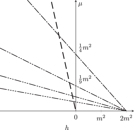
The bifurcation behaviour will be characterised in terms of the Taylor coefficients
 $m,h\in\mathbb{R}$
. The complexity of the bifurcation computations below have motivated the simplifying assumption that the third- and fourth-order coefficients vanish. Including these higher order terms would only alter the sub-/supercritical nature of the bifurcation, but not the critical values for the parameter
$m,h\in\mathbb{R}$
. The complexity of the bifurcation computations below have motivated the simplifying assumption that the third- and fourth-order coefficients vanish. Including these higher order terms would only alter the sub-/supercritical nature of the bifurcation, but not the critical values for the parameter
 $\mu$
.
$\mu$
.
4.2 Linearisation around the trivial state
In terms of a small correction
 $\bar u_1 := \bar u - \bar u_0$
, the linearisation of problem (4.1)–(4.5) reads (using (4.7))
$\bar u_1 := \bar u - \bar u_0$
, the linearisation of problem (4.1)–(4.5) reads (using (4.7))
 \begin{align} \mu\ddot \rho_1(s)-m\,\dot\theta_1(s)-\frac{h}{2}\,\rho_1(s) - \lambda_{M1} &= f(s)\,, \end{align}
 \begin{align} \frac{d}{ds}\left(\dot\theta_1(s)+m\,\rho_1(s)\right) + \lambda_{x1}\sin s - \lambda_{y1}\cos s &= g(s)\,,\end{align}
subject to the boundary conditions
 \begin{equation}\rho_{1}(2\pi) - \rho_{1}(0) = 0\,, \quad \dot\rho_{1}(2\pi) - \dot\rho_{1}(0) = 0\,, \quad \theta_{1}(0)=0\,, \quad \theta_{1}(2\pi) = 0\,,\end{equation}
the constraints
 \begin{equation}\int_0^{2\pi}\rho_1(s)\,\textrm{d} s=0 \,,\qquad \int_0^{2\pi}\begin{pmatrix}-\sin s \\ \\[-7pt] \:\:\:\cos s\end{pmatrix}\theta_1(s)\textrm{d} s=\begin{pmatrix}\alpha_x\\ \\[-7pt] \alpha_y\end{pmatrix} \,,\end{equation}
and the auxiliary condition
 \begin{equation}\rho_1(0) = 0 \,.\end{equation}
The inhomogeneities
 $f(s), g(s), \alpha_x, \alpha_y$
can be interpreted as non-linear corrections.
$f(s), g(s), \alpha_x, \alpha_y$
can be interpreted as non-linear corrections.
Proposition 4.1 (Solution of the homogeneous linearised system) A nonzero solution of (4.8)–(4.12) with
 $f=g=\alpha_x=\alpha_y=0$
,
$f=g=\alpha_x=\alpha_y=0$
,
 $\mu>0$
,
$\mu>0$
,
 $m,h\in\mathbb{R}$
, only exists in the following cases:
$m,h\in\mathbb{R}$
, only exists in the following cases:
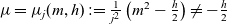
Case 1: There exists
 $j\in\mathbb{N}$
,
$j\in\mathbb{N}$
,
 $j\ge 2$
, such that
$j\ge 2$
, such that
 $\mu=\mu_j(m,h) := \frac{1}{j^2}\left(m^2-\frac{h}{2}\right) \ne -\frac{h}{2}$
. The space of solutions is one-dimensional and given by
$\mu=\mu_j(m,h) := \frac{1}{j^2}\left(m^2-\frac{h}{2}\right) \ne -\frac{h}{2}$
. The space of solutions is one-dimensional and given by
 \begin{align} \rho_1(s) = a_1 \sin(js) \,,\; \theta_1(s) = \frac{a_1 m}{j}(\cos(js)-1) \,, \nonumber \\ \lambda_{x1}=\lambda_{y1}=\lambda_{M1}=0 \,,\; a_1\in\mathbb{R}\,.\end{align}
Case 2:
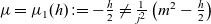 $\mu=\mu_1(h) := -\frac{h}{2}\neq\frac{1}{j^2}\left(m^2-\frac{h}{2}\right)$
for all
$\mu=\mu_1(h) := -\frac{h}{2}\neq\frac{1}{j^2}\left(m^2-\frac{h}{2}\right)$
for all
 $j\in\mathbb{N}$
,
$j\in\mathbb{N}$
,
 $j\ge 2$
. The space of solutions is one-dimensional and given by
$j\ge 2$
. The space of solutions is one-dimensional and given by
 \begin{equation} \rho_1(s) = b_1 \sin s \,,\; \theta_1(s) = 0 \,,\; \lambda_{x1}=\lambda_{M1}=0 \,,\; \lambda_{y1} = b_1 m \,,\; b_1\in\mathbb{R}\,.\end{equation}
Case 3: There exists
 $j\in\mathbb{N}$
,
$j\in\mathbb{N}$
,
 $j\ge 2$
, such that
$j\ge 2$
, such that
 $\mu=\mu_j(m,h) = \mu_1(h)$
. The space of solutions is two-dimensional and given by
$\mu=\mu_j(m,h) = \mu_1(h)$
. The space of solutions is two-dimensional and given by
 \begin{gather*} \rho_1(s) = a_1 \sin(js) + b_1 \sin s \,,\quad \theta_1(s) = \frac{a_1 m}{j}(\cos(js)-1) \,, \\ \lambda_{x1}=\lambda_{M1}=0 \,,\quad \lambda_{y1} = b_1 m \,,\qquad a_1,b_1\in\mathbb{R}\,. \end{gather*}
Remark 4.2
-
(1) As expected, bifurcations only occur under the condition (see (3.3))
 \begin{align*} 2m^2-h = 2\beta'(1)^2 - \beta(1)\beta''(1)>0 \,.\end{align*}
-
(2) For Case 1 solutions, the curvature correction
$\kappa_1 = \dot\theta_1$
satisfies
$\kappa_1 = -m\rho_1$
. This means that the sign of
$m=\beta'(1)$
decides if curvature maxima coincide with density maxima (
$m<0$
) or with density minima (
$m>0$
), which is not a surprising result. The condition
$j\ge 2$
is a manifestation of the Four Vertex Theorem (see Section 2). -
(3) Case 2 solutions exhibit only one maximum and one minimum of the density without any effect on the circular shape of the curve. The numerical computations reported in Section 5 show, however, that these solutions initiate bifurcating branches strongly deviating from the circular shape far enough from the bifurcation point.
-
(4) Whereas Cases 1 and 2 correspond to codimension-one bifurcations, Case 3 represents a bifurcation of codimension two, whose nonlinear structure will not be analyzed in the following.
-
(5) In a bifurcation scenario, where the values of m and h are fixed and the value of
$\mu$
is decreased, there are several situations. For
$h\ge2m^2$
no bifurcations occur by convexity (see above). For
$0\le h < 2m^2$
an infinite series of Case 1 bifurcations occurs at the bifurcation values
$\mu_j$
,
$j\ge 2$
, with the first one at
$\mu=\mu_2$
. For
$h<0$
, apart from the bifurcations at
$\mu=\mu_2,\mu_3,\ldots$
, there is also a Case 2 bifurcation at
$\mu=\mu_1$
. There are two subcases concerning the question, which bifurcation occurs first, determined by the criterion Codimension-two bifurcations occur whenever
\begin{align*} \mu_1 > \mu_2 \quad\Longleftrightarrow\quad h < -\frac{2}{3}m^2 \,.\end{align*}
$\mu_1=\mu_j$
, i.e.
$h = -2m^2/(j^2-1)$
for some
$j\ge 2$
. These observations are illustrated in Figure 1 in the (m,h)-plane and in Figure 2 in the (
$h\hbox{-}\mu$
)-plane.
Figure 1.Regions of different bifurcation behaviour in the (m,h)-plane according to Proposition 4.1: No bifurcations above the parabola
$h=2m^2$
. Only Case 1 bifurcations between the parabola and the m-axis. Case 1 and Case 2 bifurcations below the m axis, with codimension-two bifurcations on the parabolas
$h=-2m^2/(j^2-1)$
,
$j\ge 2$
. The first bifurcation is a Case 2 bifurcation below the parabola
$h=-2m^2/3$
, and a Case 1 bifurcation with
$j=2$
otherwise.Figure 2.Critical values of
$\mu$
for Case 1 (thin) and Case 2 (bold). The intersections correspond to (the degenerate) Case 3 which is not studied in this paper. The dashes indicate the value of j: — — for
$j=1$
, — - — for
$j=2$
, etc.


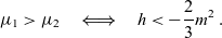


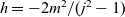


Proof. By the smoothness of solutions of ordinary differential equations, we can employ Fourier representation and write
 \begin{align*} \rho_1(s) = \sum_{k\in\mathbb{Z}} \widehat\rho_{1,k} e^{iks} \,,\qquad \theta_1(s) = \sum_{k\in\mathbb{Z}} \widehat\theta_{1,k} e^{iks} \,.\end{align*}
We keep the inhomogeneities for the moment, since this will be useful for the proof of the following result, and we use their Fourier series
 \begin{align*} f(s) = \sum_{k\in\mathbb{Z}} \widehat f_k e^{iks} \,,\qquad g(s) = \sum_{k\in\mathbb{Z}} \widehat g_k e^{iks} \,.\end{align*}
The constraints (4.11) imply
 \begin{equation} \widehat\rho_{1,0} = 0 \,,\qquad \widehat\theta_{1,\pm 1} = \frac{1}{2\pi}(\alpha_y \pm i\alpha_x) \,.\end{equation}
Comparing Fourier coefficients for
 $k=0$
in (4.8), (4.9) implies
$k=0$
in (4.8), (4.9) implies
 \begin{equation} \lambda_{M1} = -\widehat f_0 \qquad\mbox{and}\qquad \widehat g_0=0 \,,\end{equation}
where the latter has to be seen as a solvability condition for the inhomogeneous problem. Coefficients for
 $k=\pm 1$
in (4.8) and (4.9) give
$k=\pm 1$
in (4.8) and (4.9) give
 \begin{align} &-\left(\mu - \mu_1\right)\widehat\rho_{1,\pm 1} = \widehat f_{\pm 1} - \frac{m}{2\pi}(\alpha_x \mp i\alpha_y) \,,\end{align}
 \begin{align} & \pm mi \widehat\rho_{1,\pm 1} \mp \frac{i}{2}\lambda_{x1} - \frac{1}{2}\lambda_{y1} = \widehat g_{\pm 1} + \frac{1}{2\pi}(\alpha_y \pm i\alpha_x)\,.\end{align}
For coefficients with
 $|k|\ge 2$
, we obtain
$|k|\ge 2$
, we obtain
 \begin{align*} - \left( \mu k^2 + \frac{h}{2}\right)\widehat\rho_{1,k} - ikm \widehat\theta_{1,k} = \widehat f_k \,,\qquad -k^2\widehat\theta_{1,k} + ikm\widehat\rho_{1,k} = \widehat g_k \,,\end{align*}
implying
 \begin{equation} -k^2(\mu-\mu_{|k|})\widehat \rho_{1,k} = \widehat f_k - \frac{im}{k}\widehat g_k \,,\qquad \widehat\theta_{1,k} - \frac{im}{k}\widehat\rho_{1,k} = - \frac{1}{k^2}\widehat g_k\,.\end{equation}
The results follow immediately from the homogeneous (
 $f=g=\alpha_x=\alpha_y=0$
) versions of (4.15)–(4.19), using the auxiliary conditions (4.12).
$f=g=\alpha_x=\alpha_y=0$
) versions of (4.15)–(4.19), using the auxiliary conditions (4.12).
Lemma 4.3 (Solvability conditions) Case 1. Problem (4.8)–(4.12) with
 $0<\mu=\mu_j\ne\mu_1$
,
$0<\mu=\mu_j\ne\mu_1$
,
 $j\ge 2$
, has a solution if and only if
$j\ge 2$
, has a solution if and only if
 \begin{align} j{\int_0^{2\pi}{f(s)\cos(js)}\,\textrm{d} s} &= m{\int_0^{2\pi}{g(s)\sin(js)}\,\textrm{d} s} \,,\nonumber\\[3pt] j{\int_0^{2\pi}{f(s)\sin(js)}\,\textrm{d} s} &= -m{\int_0^{2\pi}{g(s)\cos(js)}\,\textrm{d} s} \,,\qquad\qquad {\int_0^{2\pi}{g(s)}\,\textrm{d} s} = 0\,.\end{align}
Case 2. Problem (4.8)–(4.12) with
 $0<\mu=\mu_1\ne\mu_j$
,
$0<\mu=\mu_1\ne\mu_j$
,
 $\forall\,j\ge 2$
, has a solution if and only if
$\forall\,j\ge 2$
, has a solution if and only if
 \begin{equation} {\int_0^{2\pi}{f(s)\cos s}\,\textrm{d} s} = m\alpha_x \,,\; {\int_0^{2\pi}{f(s)\sin s}\,\textrm{d} s} = m\alpha_y \,,\;{\int_0^{2\pi}{g(s)}\,\textrm{d} s} = 0\,.\end{equation}
Proof. For Case 1, the solvability conditions follow from (4.16), (4.19), and for Case 2 from (4.16), (4.17).
4.3 Asymptotic expansion around bifurcation points
For the codimension-one bifurcations identified above (Cases 1 and 2 in Proposition 4.1), the existence of bifurcating solution branches is guaranteed by general results on bifurcations from simple eigenvalues [Reference Crandall and Rabinowitz8]. The local shape of these branches will be analysed by perturbation expansions. By the presence of a flip symmetry in problem (4.1)–(4.5), pitchfork bifurcations can be expected, at least generically. For the bifurcation at
 $\mu=\mu_j$
,
$\mu=\mu_j$
,
 $j\in\mathbb{N}$
, we therefore introduce
$j\in\mathbb{N}$
, we therefore introduce
 \begin{align*} \mu = \mu_j - \sigma A^2 \,,\qquad 0<A\ll 1\,,\quad \sigma\in \{1,-1\} \,.\end{align*}
The small parameter A measures the distance from the bifurcation point, whereas the sign
 $\sigma$
, to be determined by the analysis, tells us whether the bifurcation is supercritical for
$\sigma$
, to be determined by the analysis, tells us whether the bifurcation is supercritical for
 $\sigma>0$
or subcritical for
$\sigma>0$
or subcritical for
 $\sigma<0$
. This convention is in line with the scenario of decreasing
$\sigma<0$
. This convention is in line with the scenario of decreasing
 $\mu$
(see Remark 4.2, 5.). The solution
$\mu$
(see Remark 4.2, 5.). The solution
 $\bar u=(\rho,\theta,\lambda_x,\lambda_y,\lambda_M)$
of (4.1)–(4.5) will be approximated by an asymptotic expansion
$\bar u=(\rho,\theta,\lambda_x,\lambda_y,\lambda_M)$
of (4.1)–(4.5) will be approximated by an asymptotic expansion
 \begin{equation} \bar u = \bar u_0 + A \bar u_1 + A^2 \bar u_2 + A^3 \bar u_3 + O(A^4) \,,\end{equation}
where the reason for going up to third order will become apparent below.
Remark 4.4 (Bifurcation diagram for classical elasticae) The expectation of pitchfork bifurcations and, thus, the ansatz (4.22) can also be motivated by the bifurcation diagram for classical elasticae (e.g. [Reference Marsden and Hughes20, Ch.7]). The diagram shows an infinite series of bifurcations similar to the series of Case 1 bifurcations in (4.1)–(4.5). In the classical elastica problem all these bifurcations are supercritical pitchforks.
The notation in (4.22) is consistent with the above. The trivial rotationally symmetric solution of (4.1)–(4.5) is denoted by
 $\bar u_0$
, and the first correction
$\bar u_0$
, and the first correction
 $\bar u_1$
has to satisfy the homogeneous version (
$\bar u_1$
has to satisfy the homogeneous version (
 $f=g=\alpha_x=\alpha_y=0$
) of the linearised problem (4.8)–(4.12) with
$f=g=\alpha_x=\alpha_y=0$
) of the linearised problem (4.8)–(4.12) with
 $\mu=\mu_j$
, whose solution is unique up to a scalar constant (
$\mu=\mu_j$
, whose solution is unique up to a scalar constant (
 $a_1$
in Case 1 and
$a_1$
in Case 1 and
 $b_1$
in Case 2). The problems for
$b_1$
in Case 2). The problems for
 $\bar u_2$
and
$\bar u_2$
and
 $\bar u_3$
are determined by substituting the ansatz (4.22) into (4.1)–(4.5), expanding the nonlinearities and comparing coefficients of
$\bar u_3$
are determined by substituting the ansatz (4.22) into (4.1)–(4.5), expanding the nonlinearities and comparing coefficients of
 $A^2$
and
$A^2$
and
 $A^3$
. Both
$A^3$
. Both
 $\bar u_2$
and
$\bar u_2$
and
 $\bar u_3$
solve inhomogeneous versions of the linearised problem (4.8)–(4.12) with
$\bar u_3$
solve inhomogeneous versions of the linearised problem (4.8)–(4.12) with
 $\mu=\mu_j$
and with the inhomogeneities
$\mu=\mu_j$
and with the inhomogeneities
 \begin{align} f_2 = \frac{m}{2}\dot\theta_1^2 + h\rho_1\dot\theta_1\,,\qquad g_2 = - \frac{d}{ds}\Big(m\rho_1\dot\theta_1+{\frac{h}{2}}\rho_1^2\Big) -\theta_1(\lambda_{x1}\cos s+\lambda_{y1}\sin s) \,,\end{align}
 \begin{align} \begin{pmatrix}\alpha_{x2}\\ \\[-7pt] \alpha_{y2}\end{pmatrix} = \frac{1}{2}{\int_0^{2\pi}{\theta_1^2\begin{pmatrix}\cos s\\ \\[-7pt] \sin s\end{pmatrix}}\,\textrm{d} s} \,,\end{align}
for
 $\bar u_2$
, and
$\bar u_2$
, and
 \begin{align}& f_3 = \sigma \ddot\rho_1 + m\dot\theta_1\dot\theta_2 + \frac{h}{2}\Big(2\rho_2\dot\theta_1+2\rho_1\dot\theta_2+\rho_1\dot\theta_1^2\Big) \,,\nonumber\\& g_3 = - \frac{d}{ds}\Big(m\rho_1\dot\theta_2+m\rho_2\dot\theta_1+\textstyle{\frac{h}{2}}\rho_1^2\dot\theta_1+h\rho_1\rho_2 \Big) \nonumber\\ &\qquad -\theta_1(\lambda_{x2}\cos s+\lambda_{y2}\sin s)-\theta_2(\lambda_{x1}\cos s+\lambda_{y1}\sin s) \end{align}
 \begin{align} +\frac{1}{2}\theta_1^2(\lambda_{x1}\sin s-\lambda_{y1}\cos s) \,,\qquad\qquad\qquad\quad \end{align}
 \begin{align} \begin{pmatrix}\alpha_{x3}\\ \\[-7pt] \alpha_{y3}\end{pmatrix} = {\int_0^{2\pi}{\begin{pmatrix}\theta_1\theta_2\cos s - \dfrac{1}{6}\theta_1^3\sin s\\ \\[-7pt] \theta_1\theta_2\sin s + \dfrac{1}{6}\theta_1^3\cos s\end{pmatrix}}\,\textrm{d} s} \,, \end{align}
for
 $\bar u_3$
. Note that the inhomogeneities depend on lower order terms. So the terms in the asymptotic expansion (4.22) can be computed recursively. However, this comes with two problems, which are connected: the solution of the linearised problem is not unique (see Proposition 4.1), and it does not have a solution for arbitrary inhomogeneities (see Lemma 4.3). The strategy is to recover the lacking information for uniqueness from the solvability conditions for higher order problems. It will turn out (as a consequence of the above mentioned flip symmetry) that the inhomogeneities (4.23), (4.24) of the second-order problem satisfy the solvability conditions, no matter what the value of the missing first-order constant (
$\bar u_3$
. Note that the inhomogeneities depend on lower order terms. So the terms in the asymptotic expansion (4.22) can be computed recursively. However, this comes with two problems, which are connected: the solution of the linearised problem is not unique (see Proposition 4.1), and it does not have a solution for arbitrary inhomogeneities (see Lemma 4.3). The strategy is to recover the lacking information for uniqueness from the solvability conditions for higher order problems. It will turn out (as a consequence of the above mentioned flip symmetry) that the inhomogeneities (4.23), (4.24) of the second-order problem satisfy the solvability conditions, no matter what the value of the missing first-order constant (
 $a_1$
in Case 1 and
$a_1$
in Case 1 and
 $b_1$
in Case 2) is. This is the reason why the third-order problem has to be considered, whose solvability condition will provide an equation for the missing first-order constant. In the following, the essential results of these straightforward but lengthy computations will be given. They have been carried out manually and checked with the help of MATHEMATICA.
$b_1$
in Case 2) is. This is the reason why the third-order problem has to be considered, whose solvability condition will provide an equation for the missing first-order constant. In the following, the essential results of these straightforward but lengthy computations will be given. They have been carried out manually and checked with the help of MATHEMATICA.
Case 1 bifurcations
The goal is to determine the value of the constant
 $a_1$
in the first-order correction
$a_1$
in the first-order correction
 $\bar u_1$
of the expansion (4.22), given in (4.13). The first step is the computation of the second-order terms.
$\bar u_1$
of the expansion (4.22), given in (4.13). The first step is the computation of the second-order terms.
Lemma 4.5 (Case 1: second-order solution) Let
 $j\ge 2$
and
$j\ge 2$
and
 $\bar u_1$
be given by (4.13). Then every solution of (4.8)–(4.12) with
$\bar u_1$
be given by (4.13). Then every solution of (4.8)–(4.12) with
 $0<\mu=\mu_j\ne\mu_1$
and with the inhomogeneities given by (4.23), (4.24) can be written as
$0<\mu=\mu_j\ne\mu_1$
and with the inhomogeneities given by (4.23), (4.24) can be written as
 \begin{align}& \rho_2(s)=a_2\sin(js) + \frac{a_1^2(m(m^2-h))}{2(2m^2-h)}(\cos(2js)-\cos(js)) \,,\nonumber\\& \theta_2(s)={a_2 \frac{m}{j}(\cos(js)-1)-\frac{a_1^2(6m^4-6m^2h+h^2)}{8j(2m^2-h)}\sin(2js)} \,,\qquad a_2\in\mathbb{R}\,,\nonumber\\[3pt] & \lambda_{x2}=\lambda_{y2}=0,\quad{\lambda_{M2}=-\frac{a_1^2 m(m^2-2h)}{4}} \,.\end{align}
Lemma 4.6 (Case 1: the missing constant) Let
 $j\ge 2$
,
$j\ge 2$
,
 $0<\mu_j\ne\mu_1$
, and
$0<\mu_j\ne\mu_1$
, and
 $\bar u_1, \bar u_2$
be given by (4.13), (4.28). Then the inhomogeneities given by (4.25)–(4.27) satisfy the solvability conditions (4.20), if and only if
$\bar u_1, \bar u_2$
be given by (4.13), (4.28). Then the inhomogeneities given by (4.25)–(4.27) satisfy the solvability conditions (4.20), if and only if
 \begin{equation}a_1\left(j^2\sigma - a_1^2\frac{Z(m,h)}{8(2m^2-h)}\right)=0 \,,\qquad\text{with}\quad Z(m,h):=-14m^6+36m^4h-18m^2h^2+h^3 \,.\quad\end{equation}
This shows that Case 1 bifurcations are pitchforks if and only if
 $Z(m,h)\ne 0$
. The amplitude of the first-order term along the bifurcating branch is determined by the nontrivial solutions of (4.29):
$Z(m,h)\ne 0$
. The amplitude of the first-order term along the bifurcating branch is determined by the nontrivial solutions of (4.29):
 \begin{equation}a_1^2=\frac{8j^2\sigma(2m^2-h)}{Z(m,h)} \,,\end{equation}
which shows for the criticality
 $\sigma = \mbox{sign }Z(m,h)$
that the bifurcation is supercritical for
$\sigma = \mbox{sign }Z(m,h)$
that the bifurcation is supercritical for
 $Z(m,h)>0$
and subcritical for
$Z(m,h)>0$
and subcritical for
 $Z(m,h)<0$
. Writing
$Z(m,h)<0$
. Writing
 $Z(m,h)=m^6(z^3-18z^2+36z-14)$
with
$Z(m,h)=m^6(z^3-18z^2+36z-14)$
with
 $z:=h/m^2<2$
shows that
$z:=h/m^2<2$
shows that
 $Z(m,h)>0$
and
$Z(m,h)>0$
and
 $2m^2>h$
are equivalent to
$2m^2>h$
are equivalent to
 \begin{equation}z_1<z<z_2\quad\text{with}\quad z_1\approx 0.52\quad\text{and}\quad z_2\approx 1.71.\end{equation}
Consequently, a supercritical pitchfork bifurcation occurs in the parabolic region
 \begin{align*} \{(m,h)\in{\mathbb{R}}^2:\:z_1m^2<h<z_2m^2\}.\end{align*}
Conversely, if (m,h) is such that
 $Z(m,h)<0$
, which holds for
$Z(m,h)<0$
, which holds for
 $h<z_1m^2$
or
$h<z_1m^2$
or
 $2m^2>h>z_2m^2$
, then the bifurcation is subcritical. The situation is illustrated in Figure 3. Note that the criticality is independent from j. For a fixed pair (m,h), the whole series of Case 1 bifurcations has the same criticality.
$2m^2>h>z_2m^2$
, then the bifurcation is subcritical. The situation is illustrated in Figure 3. Note that the criticality is independent from j. For a fixed pair (m,h), the whole series of Case 1 bifurcations has the same criticality.
Contour plot of Z(m,h) given by (4.29). The solution in Case 1 has the structure of a supercritical pitchfork bifurcation whenever
 $Z(m,h)>0$
and
$Z(m,h)>0$
and
 $h<2m^2$
. These conditions define the crosshatched region
$h<2m^2$
. These conditions define the crosshatched region
 $z_1m^2<h<z_2m^2$
below the parabola
$z_1m^2<h<z_2m^2$
below the parabola
 $h=2m^2$
(black line);
$h=2m^2$
(black line);
 $z_1\approx 0.52$
and
$z_1\approx 0.52$
and
 $z_2\approx 1.71$
, see (4.31). Conversely, if
$z_2\approx 1.71$
, see (4.31). Conversely, if
 $Z(m,h)<0$
which is true when
$Z(m,h)<0$
which is true when
 $h<z_1m^2$
or in the narrow white region given by
$h<z_1m^2$
or in the narrow white region given by
 $z_2m^2<h<2m^2$
, then the bifurcation is subcritical.
$z_2m^2<h<2m^2$
, then the bifurcation is subcritical.

Case 2 bifurcations
Lemma 4.7 (Case 2: second-order solution) Let
 $\bar u_1$
be given by (4.14). Then every solution of (4.8)–(4.12) with
$\bar u_1$
be given by (4.14). Then every solution of (4.8)–(4.12) with
 $0<\mu=\mu_1\ne\mu_j$
,
$0<\mu=\mu_1\ne\mu_j$
,
 $\forall j\ge 2$
, and with the inhomogeneities given by (4.23), (4.24) can be written as
$\forall j\ge 2$
, and with the inhomogeneities given by (4.23), (4.24) can be written as
 \begin{align}& \rho_2(s)=b_2\sin s + \frac {b_1^2 mh}{2(2m^2+3h)} (\cos(2s)-\cos s) \,,\qquad b_2\in\mathbb{R}\,,\nonumber\\[3pt]& \theta_2(s)=\frac{b_1^2 3h^2}{8(2m^2+3h)} \sin(2s) \,,\\[3pt] & \lambda_{x2}= -\frac{b_1^2 m^2 h}{2(2m^2+3h)}\,,\quad \lambda_{y2}=b_2 m \,,\quad \lambda_{M2}=0 \,.\nonumber\end{align}
Lemma 4.8 (Case 2: the missing constant) Let
 $0<\mu_1\ne\mu_j$
,
$0<\mu_1\ne\mu_j$
,
 $\forall j\ge 2$
, and
$\forall j\ge 2$
, and
 $\bar u_1, \bar u_2$
be given by (4.14), (4.32). Then the inhomogeneities given by (4.25)–(4.27) satisfy the solvability conditions (4.21), if and only if
$\bar u_1, \bar u_2$
be given by (4.14), (4.32). Then the inhomogeneities given by (4.25)–(4.27) satisfy the solvability conditions (4.21), if and only if
 \begin{equation}b_1\Big(\sigma +b_1^2\,\frac{3h^3}{8(2m^2+3h)}\Big)=0 \,.\quad\end{equation}
This shows that Case 2 bifurcations are pitchforks, since
 \begin{align*} b_1^2 = -\frac{8\sigma(2m^2+3h)}{3h^3} \,\end{align*}
is finite by
 $\mu_1 = -h/2 >0$
and nonvanishing by
$\mu_1 = -h/2 >0$
and nonvanishing by
 $2m^2+3h = 8(\mu_2-\mu_1) \ne 0$
. The bifurcation is subcritical for
$2m^2+3h = 8(\mu_2-\mu_1) \ne 0$
. The bifurcation is subcritical for
 $2m^2+3h<0$
, i.e. when the Case 2 bifurcation is the first one for decreasing
$2m^2+3h<0$
, i.e. when the Case 2 bifurcation is the first one for decreasing
 $\mu$
(see Remark 4.2, 5.). It is supercritical for
$\mu$
(see Remark 4.2, 5.). It is supercritical for
 $2m^2+3h>0$
. It is also noteworthy that the circular shape of the trivial solution curve is now perturbed at the order of
$2m^2+3h>0$
. It is also noteworthy that the circular shape of the trivial solution curve is now perturbed at the order of
 $A^2$
with the perturbation given in (4.32). The leading order density perturbation
$A^2$
with the perturbation given in (4.32). The leading order density perturbation
 $\rho_1$
has both its extrema coinciding either with the maxima of the curvature perturbation
$\rho_1$
has both its extrema coinciding either with the maxima of the curvature perturbation
 $\dot\theta_2$
(in the subcritical case) or with its minima (in the supercritical case). This can be verified numerically, see Cases (iv) and (v) in Section 5.3 and Figure 6 for
$\dot\theta_2$
(in the subcritical case) or with its minima (in the supercritical case). This can be verified numerically, see Cases (iv) and (v) in Section 5.3 and Figure 6 for
 $j=1$
.
$j=1$
.
4.4 Energy and stability
As an indicator for the stability of bifurcating solutions, we investigate the changes of the energy (1.1) along bifurcating branches. For this purpose, we substitute
 $\mu = \mu_j - \sigma A^2$
and the asymptotic expansion (4.22) of the bifurcating solution into the energy and re-expand:
$\mu = \mu_j - \sigma A^2$
and the asymptotic expansion (4.22) of the bifurcating solution into the energy and re-expand:
 \begin{align*}E_\mu(\rho,\theta)=\frac{1}{2}\int_0^{2\pi}(\beta(\rho)\,\dot\theta^2+\mu\dot\rho^2)\,\textrm{d} s=E_0+AE_1+A^2E_2+A^3E_3+A^4E_4+ O(A^5) \,.\end{align*}
For the coefficients, we obtain (all computations of this section were again verified with MATHEMATICA)
 \begin{align}E_0&=\frac{1}{2}\int_0^{2\pi}\textrm{d} s=\pi=E_{\mu_j}(\rho_0,\theta_0) \,,\qquad E_1=\frac{1}{2}\int_0^{2\pi}\left(m\rho_1+2\dot\theta_1\right)\textrm{d} s = 0 \,,\end{align}
 \begin{align}E_2&=\frac{1}{2}\int_0^{2\pi}\left(2m\rho_1\dot\theta_1+\textstyle{\frac{h}{2}}\rho_1^2+\dot\theta_1^2+\mu_j\dot\rho_1^2\right)\textrm{d} s \,,\end{align}
 \begin{align}E_3&=\frac{1}{2}\int_0^{2\pi}\left(2m\rho_1\dot\theta_2+2m\rho_2\dot\theta_1+m\rho_1\dot\theta_1^2 +h\rho_1\rho_2+h\rho_1^2\dot\theta_1+ 2 \dot\theta_1\dot\theta_2 +2\mu_j\dot\rho_1 \dot\rho_2\right)\textrm{d} s \,,\end{align}
 \begin{align}E_4&=\frac{1}{2}\int_0^{2\pi}\biggl(2m\rho_1\dot\theta_3+2m\rho_3\dot\theta_1+ m\rho_2\dot\theta_1^2+2m\rho_2\dot\theta_2+2m\rho_1\dot\theta_1\dot\theta_2+\frac{h}{2}\rho_2^2+h\rho_1\rho_3\nonumber\\&+2h\rho_1\rho_2\dot\theta_1+{\frac{h}{2}}\rho_1^2\dot\theta_1^2+h\rho_1^2\dot\theta_2+2 \dot\theta_1 \dot\theta_3+\dot\theta_2^2+\mu_j\dot\rho_2^2 +2\mu_j\dot\rho_1 \dot\rho_3-\sigma\dot\rho_1^2\biggr)\textrm{d} s \,.\end{align}
Lemma 4.9 (Energy expansion) Let
 $j\in\mathbb{N}$
, let
$j\in\mathbb{N}$
, let
 $\bar u_1,\bar u_2$
be given by (4.13), (4.28) in Case 1,
$\bar u_1,\bar u_2$
be given by (4.13), (4.28) in Case 1,
 $j\ge 2$
, or by (4.14), (4.32) in Case 2,
$j\ge 2$
, or by (4.14), (4.32) in Case 2,
 $j=1$
. Let the constants
$j=1$
. Let the constants
 $a_1$
in Case 1 or
$a_1$
in Case 1 or
 $b_1$
in Case 2 be chosen such that the third-order inhomogeneities (4.25)–(4.27) satisfy the solvability conditions of Lemma 4.6 in Case 1 and Lemma 4.8 in Case 2. Let
$b_1$
in Case 2 be chosen such that the third-order inhomogeneities (4.25)–(4.27) satisfy the solvability conditions of Lemma 4.6 in Case 1 and Lemma 4.8 in Case 2. Let
 $\bar u_3$
be a corresponding solution of the linearised problem (4.8)–(4.12) with
$\bar u_3$
be a corresponding solution of the linearised problem (4.8)–(4.12) with
 $\mu=\mu_j$
. Then the coefficients in the energy expansion above satisfy
$\mu=\mu_j$
. Then the coefficients in the energy expansion above satisfy
 $E_1=E_2=E_3=0$
in both cases, as well as
$E_1=E_2=E_3=0$
in both cases, as well as
 \begin{equation}E_{4}=-\frac{2\pi j^4(2m^2-h)}{Z(m,h)}\end{equation}
in Case 1 with the notation of Lemma 4.6. In Case 2, we have
 \begin{align*}E_4=\frac{2\pi (3h+2m^2)}{3h^3} \,.\end{align*}
As expected, the sign of
 $E_4$
goes with criticality of the bifurcating branch. Stability is gained (
$E_4$
goes with criticality of the bifurcating branch. Stability is gained (
 $E_4<0$
) along supercritical branches and lost (
$E_4<0$
) along supercritical branches and lost (
 $E_4>0$
) along subcritical branches. In particular, this can be expected to decide the stability of the branch corresponding to the first bifurcation for decreasing
$E_4>0$
) along subcritical branches. In particular, this can be expected to decide the stability of the branch corresponding to the first bifurcation for decreasing
 $\mu$
.
$\mu$
.
5 Numerical continuation of bifurcation branches
5.1 Discretisation
The Euler–Lagrange equations (4.1) and (4.2) are discretised by finite differences as follows. For
 $N\in\mathbb{N}$
, we discretise the interval [0,L] by introducing
$N\in\mathbb{N}$
, we discretise the interval [0,L] by introducing
 $\Delta s = L (N-1)^{-1}$
and
$\Delta s = L (N-1)^{-1}$
and
 $s_i = i \Delta s$
,
$s_i = i \Delta s$
,
 $0 \le i \le N-1$
, which naturally leads to the (abuse of) notation
$0 \le i \le N-1$
, which naturally leads to the (abuse of) notation
 $\rho=({\rho}_i)_{i=1}^{N-1}$
,
$\rho=({\rho}_i)_{i=1}^{N-1}$
,
 $\theta=({\theta}_i)_{i=1}^{N-1}$
with
$\theta=({\theta}_i)_{i=1}^{N-1}$
with
 ${\rho}_i = \rho(s_i)$
,
${\rho}_i = \rho(s_i)$
,
 ${\theta}_i = \theta(s_i)$
. This can be thought of as considering a polygonal approximation of the curve
${\theta}_i = \theta(s_i)$
. This can be thought of as considering a polygonal approximation of the curve
 $\gamma$
, where
$\gamma$
, where
 $\theta_i$
is the angle of the ith side and where
$\theta_i$
is the angle of the ith side and where
 $\rho_i$
is a piecewise constant approximation of
$\rho_i$
is a piecewise constant approximation of
 $\rho$
on that side (i.e.
$\rho$
on that side (i.e.
 $\rho_i$
is not associated to a vertex).
$\rho_i$
is not associated to a vertex).
Using the notation
 $u = (\rho, \theta)$
and
$u = (\rho, \theta)$
and
 $\Lambda=(\lambda_x,\lambda_y,\lambda_M)$
, we propose the following natural finite differences approximation for (4.1) and (4.2), respectively:
$\Lambda=(\lambda_x,\lambda_y,\lambda_M)$
, we propose the following natural finite differences approximation for (4.1) and (4.2), respectively:
 \begin{align} EL_\rho(u, \Lambda) &= \mu \left(\frac{\rho_{i-1} - 2 \rho_i + \rho_{i+1}}{\Delta s^2}\right) - \frac{1}{2} \beta'(\rho_i) \left(\frac{\rho_{i+1} - \rho_{i-1}}{2 \Delta s}\right)^2 - \lambda_M = 0\,, \end{align}
 \begin{align} EL_\theta(u, \Lambda) &= \frac{1}{\Delta s}\left(\beta\left(\frac{\rho_{i+1}+\rho_i}{2}\right)\left(\frac{\theta_{i+1} - \theta_{i}}{\Delta s}\right) - \beta\left(\frac{\rho_{i}+\rho_{i-1}}{2}\right) \left(\frac{\theta_{i} - \theta_{i-1}}{\Delta s}\right)\right) \nonumber \\[3pt] & \quad + \lambda_x \sin \theta_i - \lambda_y \cos \theta_i = 0\,, \end{align}
for
 $0 \le i \le N-1$
.
$0 \le i \le N-1$
.
To remove the degree of freedom associated to solid rotations, we can set
 $\theta(0) = 0$
at the continuous level. This is reflected by the choice
$\theta(0) = 0$
at the continuous level. This is reflected by the choice
 $\theta_0 = 0$
at the discrete level. We also need to provide values for indices
$\theta_0 = 0$
at the discrete level. We also need to provide values for indices
 $i = {-1, N}$
. Again by periodicity we set
$i = {-1, N}$
. Again by periodicity we set
 $\rho_{-1} = \rho_{N-1}$
,
$\rho_{-1} = \rho_{N-1}$
,
 $\rho_{N} = \rho_0$
,
$\rho_{N} = \rho_0$
,
 $\theta_{-1} = \theta_{N-1} - 2\pi$
, and
$\theta_{-1} = \theta_{N-1} - 2\pi$
, and
 $\theta_{N} = \theta_0 + 2\pi$
. Thus, we only consider (5.1) for
$\theta_{N} = \theta_0 + 2\pi$
. Thus, we only consider (5.1) for
 $0 \le i < N-1$
and (5.2) for
$0 \le i < N-1$
and (5.2) for
 $0 < i < N-1$
.
$0 < i < N-1$
.
The mass and closedness constraints can be naturally approximated as
 \begin{align*} C_M(u, \Lambda) &= \Delta s \sum_{i=0}^{N-1} \rho_i - M = 0\,,\\[3pt] \begin{pmatrix} C_{x}\\ \\[-7pt] C_{y}\end{pmatrix}(u, \Lambda) &= \Delta s \sum_{i=0}^{N-1} \begin{pmatrix}\cos \theta_i \\ \\[-7pt] \sin \theta_i\end{pmatrix} = 0\,.\end{align*}
We are left with a system of
 $2N + 1$
nonlinear equations which we propose to solve using a damped Newton method. If we assume
$2N + 1$
nonlinear equations which we propose to solve using a damped Newton method. If we assume
 $\bar{u}^k = \left(u^k, \Lambda^k\right)$
to be known, we look for
$\bar{u}^k = \left(u^k, \Lambda^k\right)$
to be known, we look for
 $\bar{u}^{k+1}$
as a solution to
$\bar{u}^{k+1}$
as a solution to
 \begin{equation} J(\bar{u}^k)\, (\bar{u}^{k+1} - \bar{u}^k) = - \eta\, r(\bar{u}^k)\,,\end{equation}
where
 $r(\bar{u}^k) = \left(EL_\rho, EL_\theta, C_x, C_y, C_M\right)$
, J is the Jacobian of r with respect to
$r(\bar{u}^k) = \left(EL_\rho, EL_\theta, C_x, C_y, C_M\right)$
, J is the Jacobian of r with respect to
 $\bar{u}$
, and
$\bar{u}$
, and
 $\eta \le 1$
is the damping parameter with
$\eta \le 1$
is the damping parameter with
 $\eta = 1$
corresponding to the standard Newton’s method.
$\eta = 1$
corresponding to the standard Newton’s method.
5.1.1 Continuation of branches
To follow numerically the bifurcation branches, one can pick some
 $\mu$
close to the critical value
$\mu$
close to the critical value
 $\mu_j$
and take as initial value a perturbation of the trivial solution (corresponding to the circle with homogeneous
$\mu_j$
and take as initial value a perturbation of the trivial solution (corresponding to the circle with homogeneous
 $\rho$
). The position of
$\rho$
). The position of
 $\mu$
relative to the critical value and the amplitude of the bifurcation are given precisely by the results of Section 4. Solving (5.3) yields a numerical approximation of a critical point, which can be used as initial condition for neighbouring values of
$\mu$
relative to the critical value and the amplitude of the bifurcation are given precisely by the results of Section 4. Solving (5.3) yields a numerical approximation of a critical point, which can be used as initial condition for neighbouring values of
 $\mu$
. By iterating this process, one can move along the branch, provided that
$\mu$
. By iterating this process, one can move along the branch, provided that
-
(1) the branch is locally smooth (for example, this is not the case when
$\rho$
hits zeros of
$\beta$
, where one could expect the branch to terminate), -
(2) the features of the solution can be resolved by the discretisation with the chosen value of N.


5.2 Choice of parameters
In what follows we will consider a number of different situations, depending on the choice of parameters (m, h) for the function
 $\beta$
, which will be of the form (4.7) with
$\beta$
, which will be of the form (4.7) with
 $\beta_0=1$
, namely
$\beta_0=1$
, namely
 \begin{equation*} \beta(\rho) = 1 + m\left(\rho - \rho_0\right) + \frac{h}{2} \left(\rho-\rho_0\right)^2.\end{equation*}
As before we will take
 $M = L = 2\pi$
, so that
$M = L = 2\pi$
, so that
 $\rho_0 = 1$
. We consider six sets of parameters:
$\rho_0 = 1$
. We consider six sets of parameters:
-
(i)
$(m,h) = (1,1.85)$
corresponding to Case 1 with
$\sigma = -1$
(subcritical bifurcation), -
(ii)
$(m,h) = (1,1)$
corresponding to Case 1 with
$\sigma = 1$
(supercritical bifurcation), -
(iii)
$(m,h) = (1,1/4)$
corresponding to Case 1 with
$\sigma = -1$
(subcritical bifurcation), -
(iv)
$(m,h) = (1, -1/2)$
corresponding to Case 1 with
$\sigma = -1$
(subcritical bifurcation) and supercritical Case 2, -
(v)
$(m,h) = (1, -2)$
corresponding to Case 1 with
$\sigma = -1$
(subcritical bifurcation) and subcritical Case 2, -
(vi)
$(m,h) = (0, -1)$
, which is similar to (v) in the special choice
$m=0$
. At first order,
$\gamma$
should remain a circle, including for Case 1, as the correction coefficient
$\theta_1 \equiv 0$
for
$m=0$
, see (4.13).


For the definition of the different cases, we refer to Proposition 4.1. The parameters in (i)–(vi) are represented in Figure 4. The corresponding results are presented in Figures 5 and 6.
The different sets of model parameters (m,h) represented on the parameter space. The grey region corresponds to parameters which have no critical points except the trivial solution. The crosshatched region corresponds to supercritical bifurcations (Case 1 for
 $h>0$
, Case 2 for
$h>0$
, Case 2 for
 $h<0$
), and the plain white region to subcritical bifurcations. The dashed parabolas indicate where Case 3 occurs, for j up to 8.
$h<0$
), and the plain white region to subcritical bifurcations. The dashed parabolas indicate where Case 3 occurs, for j up to 8.

Numerical results for Cases (i) to (vi), in columns, for
 $j=1,2,3$
. The first column shows the amplitude in
$j=1,2,3$
. The first column shows the amplitude in
 $\rho$
, where the lower and greatest values of
$\rho$
, where the lower and greatest values of
 $\rho$
are represented. The horizontal grey line corresponds to the trivial solution, for which
$\rho$
are represented. The horizontal grey line corresponds to the trivial solution, for which
 $\rho \equiv 1$
. The second column shows the energy
$\rho \equiv 1$
. The second column shows the energy
 $E_\mu$
, with the horizontal grey line again corresponding to the trivial solution, for which
$E_\mu$
, with the horizontal grey line again corresponding to the trivial solution, for which
 $E_\mu = \pi$
. The dashes indicate the value of j for each branch: — — for
$E_\mu = \pi$
. The dashes indicate the value of j for each branch: — — for
 $j=1$
(absent in (i) to (iii)), — - — for
$j=1$
(absent in (i) to (iii)), — - — for
 $j=2$
, — - - — for
$j=2$
, — - - — for
 $j=3$
. The grey vertical lines indicate the theoretical critical values for
$j=3$
. The grey vertical lines indicate the theoretical critical values for
 $\mu$
. In Cases (i) to (iii), the secondary bifurcation branch is plotted in gray. As detailed in (4.22), at a supercritical (resp. subcritical) bifurcation point, the branch will appear for values of
$\mu$
. In Cases (i) to (iii), the secondary bifurcation branch is plotted in gray. As detailed in (4.22), at a supercritical (resp. subcritical) bifurcation point, the branch will appear for values of
 $\mu$
greater (resp. lower) than the critical value.
$\mu$
greater (resp. lower) than the critical value.

The shapes corresponding to each case, with
 $j = 1,2,3$
increasing with each column. These correspond to the last point computed on the branches shown in Figure 5. In Cases (i) to (iii), the shapes in the first column are in grey, as they do not correspond to branches bifurcating from the trivial state, and j is not defined in this case. They are placed in the first column due to their resemblance to shapes obtained for
$j = 1,2,3$
increasing with each column. These correspond to the last point computed on the branches shown in Figure 5. In Cases (i) to (iii), the shapes in the first column are in grey, as they do not correspond to branches bifurcating from the trivial state, and j is not defined in this case. They are placed in the first column due to their resemblance to shapes obtained for
 $h < 0$
, in Cases (iv) to (vi). Thicker lines denote larger values of
$h < 0$
, in Cases (iv) to (vi). Thicker lines denote larger values of
 $\rho$
.
$\rho$
.

5.3 Results
The method described above (Section 5.1) was implemented in Julia [Reference Bezanson, Edelman, Karpinski and Shah4]. Figure 5 presents the bifurcating branches both in terms of the amplitude of the density
 $\rho$
and in terms of the energy
$\rho$
and in terms of the energy
 $E_\mu$
. It offers a partial confirmation of the results of Section 4 in that:
$E_\mu$
. It offers a partial confirmation of the results of Section 4 in that:
-
• For Case (ii),
$j \ge 2$
and (iv),
$j = 1$
, the bifurcation appears supercritical, i.e., the branch bifurcates to the left of the critical
$\mu$
. Additionally, the energy decreases close to the trivial state. These branches offer critical points of
$E_\mu$
which are candidates to be global minimisers. -
• For all other cases, the bifurcation is subcritical, i.e., the branch bifurcates to the right of the critical
$\mu$
, and the energy initially increases as one gets further from the trivial state.


Interestingly, Cases (i) and (iv) feature turning points, where the derivative of
 $E_\mu$
along the branch seems to change sign. In Case (i) it becomes negative, leading to critical points of lower energy with respect to the trivial state, and potentially global minimisers. This fact precludes uniqueness of minimisers of
$E_\mu$
along the branch seems to change sign. In Case (i) it becomes negative, leading to critical points of lower energy with respect to the trivial state, and potentially global minimisers. This fact precludes uniqueness of minimisers of
 $E_\mu$
in general.
$E_\mu$
in general.
We were able to track an additional branch in Cases (i) to (iii), which seems to bifurcate from the
 $j=2$
branch. No analytical results are available at this point, but we can make the following observations. The corresponding shapes, presented in grey in Figure 6, look like the ones obtained for
$j=2$
branch. No analytical results are available at this point, but we can make the following observations. The corresponding shapes, presented in grey in Figure 6, look like the ones obtained for
 $j=1$
in Cases (iv) to (vi). This justifies the placement in the first column, although j has no meaning for this branch. In Cases (i) and (iii), it bifurcates from the
$j=1$
in Cases (iv) to (vi). This justifies the placement in the first column, although j has no meaning for this branch. In Cases (i) and (iii), it bifurcates from the
 $j=2$
branch with decreasing energy for the choice of parameter considered. Case (ii) is a bit different, in that the bifurcation leads to critical points of higher energy, although the branch features a turning point, after which
$j=2$
branch with decreasing energy for the choice of parameter considered. Case (ii) is a bit different, in that the bifurcation leads to critical points of higher energy, although the branch features a turning point, after which
 $E_\mu$
starts decreasing and eventually becomes smaller than for the
$E_\mu$
starts decreasing and eventually becomes smaller than for the
 $j=2$
branch, for a given value of
$j=2$
branch, for a given value of
 $\mu$
.
$\mu$
.
Other features of the critical points further along the branch can be seen in Figure 6. For Cases (i) to (v) and
 $j>1$
, one can identify the value of j with the number of flatter sections in each closed curve. These correspond to higher values of
$j>1$
, one can identify the value of j with the number of flatter sections in each closed curve. These correspond to higher values of
 $\rho$
, which agree with the fact that for all choices of parameters presented here,
$\rho$
, which agree with the fact that for all choices of parameters presented here,
 $m\ge0$
. This can be roughly thought as higher values of
$m\ge0$
. This can be roughly thought as higher values of
 $\rho$
penalising higher values of the curvature
$\rho$
penalising higher values of the curvature
 $\dot\theta$
. For
$\dot\theta$
. For
 $j=1$
or in Case (vi), the situation is different, since the first-order correction
$j=1$
or in Case (vi), the situation is different, since the first-order correction
 $\theta_1 \equiv 0$
. If one goes further in the expansion, one can expect that the next-order correction
$\theta_1 \equiv 0$
. If one goes further in the expansion, one can expect that the next-order correction
 $\theta_2$
have the form
$\theta_2$
have the form
 $\cos(2js)$
, that is half the period of
$\cos(2js)$
, that is half the period of
 $\rho_1$
. This could explain that in these cases,
$\rho_1$
. This could explain that in these cases,
 $\rho$
seems to have j maxima when
$\rho$
seems to have j maxima when
 $\dot\theta$
has 2j.
$\dot\theta$
has 2j.
Additionally, far from the bifurcation point and after potential turning points, one can distinguish Cases (i) and (ii) from Cases (iii) to (vi). For the former,
 $\mu$
decreases along the branch,
$\mu$
decreases along the branch,
 $E_\mu$
decreases and
$E_\mu$
decreases and
 $\rho$
seems to concentrate on flat sections. For the latter, the situation is the opposite:
$\rho$
seems to concentrate on flat sections. For the latter, the situation is the opposite:
 $\mu$
increases along the branch,
$\mu$
increases along the branch,
 $E_\mu$
increases and
$E_\mu$
increases and
 $\rho$
stays rather smooth.
$\rho$
stays rather smooth.
Remark 5.1 In Proposition 3.3 it is stated that for
 $\beta$
bounded away from 0, only the trivial state
$\beta$
bounded away from 0, only the trivial state
 $(\rho_0, \theta_0)$
is a minimiser of
$(\rho_0, \theta_0)$
is a minimiser of
 $E_\mu$
. The branches in Figure 5 which seem to continue far to large values of
$E_\mu$
. The branches in Figure 5 which seem to continue far to large values of
 $\mu$
have an energy clearly larger than
$\mu$
have an energy clearly larger than
 $\pi = E_\mu(\rho_0, \theta_0)$
. We also recall that for the results presented here, the choice of
$\pi = E_\mu(\rho_0, \theta_0)$
. We also recall that for the results presented here, the choice of
 $\beta$
is quadratic, and thus not bounded away from 0. There is then no contradiction of our analysis.
$\beta$
is quadratic, and thus not bounded away from 0. There is then no contradiction of our analysis.
A systematic study of the stability in terms of the energy would be interesting, although probably necessarily limited to numerics, as it would help identifying local minimisers. Such an investigation is however out of the scope of this paper.
6 Conclusion
To describe elastic curves in the plane, we introduced a regularised Canham–Helfrich type functional which includes a density-modulated stiffness
 $\beta$
. We proved that the associated minimisation problem has a solution if the regularisation parameter is positive. If not, the problem has no solution in general. Conditions on the first derivatives of
$\beta$
. We proved that the associated minimisation problem has a solution if the regularisation parameter is positive. If not, the problem has no solution in general. Conditions on the first derivatives of
 $\beta$
were derived so that the problem has non-trivial solutions. In this case, a bifurcation analysis around the trivial solution was performed, the regularisation parameter playing the role of the bifurcation parameter. A family of both subcritical and supercritical pitchfork bifurcations was found, depending on the choice of
$\beta$
were derived so that the problem has non-trivial solutions. In this case, a bifurcation analysis around the trivial solution was performed, the regularisation parameter playing the role of the bifurcation parameter. A family of both subcritical and supercritical pitchfork bifurcations was found, depending on the choice of
 $\beta$
. This contrasts with the classical elastic curves, which display supercritical bifurcations only. An expansion of the energy confirmed that subcritical (resp. supercritical) solutions correspond to a gain (resp. a loss) of energy compared to the trivial state. This analysis was completed by numerical continuation of the bifurcating branches, which confirmed the theoretical findings. Secondary bifurcations and turning points – found numerically – testify of the intricate mathematical structure of the model. In particular, no uniqueness should be expected for the minimisation problem, except for large regularisation.
$\beta$
. This contrasts with the classical elastic curves, which display supercritical bifurcations only. An expansion of the energy confirmed that subcritical (resp. supercritical) solutions correspond to a gain (resp. a loss) of energy compared to the trivial state. This analysis was completed by numerical continuation of the bifurcating branches, which confirmed the theoretical findings. Secondary bifurcations and turning points – found numerically – testify of the intricate mathematical structure of the model. In particular, no uniqueness should be expected for the minimisation problem, except for large regularisation.
Acknowledgements
This work has been supported by the Austrian Science Fund (FWF) projects F 65, W 1245, P 32788, by the Vienna Science and Technology Fund (WWTF) through Project MA14-009, and by the Austrian Academy of Sciences via the New Frontier’s grant NST 0001.