


1. Introduction
Confirmation theory studies the formal patterns of how (and how much) evidence speaks in favor of or against hypotheses. Contrary to deductive logic, it allows for nuanced assessments of hypotheses in light of the evidence. This makes confirmation theory central to the epistemological dimension of the philosophy of science, for it is the exception, and not the rule, that the evidence logically entails a scientific hypothesis of interest or its negation.
The logical empiricists took two distinct approaches to confirmation theory. The first, championed by Hempel, studied confirmation qualitatively. It asked under which conditions evidence can be said to confirm or disconfirm a hypothesis (Hempel Reference Hempel1945). The second, championed by Carnap, studied confirmation quantitatively. It asked to what degree a hypothesis is confirmed by the evidence (Carnap Reference Carnap1962). This article is concerned with the quantitative notion.
Quantitative confirmation is generally understood in one of two ways: either incrementally as “increase in firmness” or absolutely as “firmness” of a hypothesis in view of the evidence (Carnap Reference Carnap1962, xvi). While I shall consider confirmation in the absolute sense, my considerations may be relevant for the incremental conception too, since incremental confirmation can be seen as measuring changes in absolute confirmation.
It is commonplace to represent degrees of confirmation by conditional probabilities of hypotheses on the evidence. Axiomatic characterizations of degrees of confirmation are usually directly modeled after the axioms of conditional probability. This is as true for the pioneering work of Hosiasson-Lindenbaum (Reference Hosiasson-Lindenbaum1940), who drew on Mazurkiewicz’s conditional probability axioms, as it is for contemporary textbook accounts (notably Hawthorne Reference Hawthorne, Prasanta and Malcolm2011). For Carnap (Reference Carnap1945, Reference Carnap1962), “degree of confirmation” referred to the same concept as “logical probability”; this made it natural for him to explicate it in accordance with the mathematical probability calculus. And even though most proponents of the now dominant Bayesian mainstream identify (or replace) degrees of confirmation with rational degrees of belief, these are likewise assumed to behave like conditional probabilities by virtue of Bayes’ rule (Howson and Urbach Reference Howson and Urbach2006).Footnote 1
The philosophical justifications for representing degrees of confirmation with conditional probabilities fall into two groups. The first, studying confirmation independently of (or prior to) rational belief, has largely followed Carnap in motivating probabilities by way of explication (see, e.g., Maher Reference Maher and Hitchcock2004; Hawthorne Reference Hawthorne, Prasanta and Malcolm2011). Probabilities—in the mathematical sense—are argued to provide an adequate and particularly fruitful precisification (explicatum) of the pretheoretic concept of “confirmation” (the explicandum). The second group, studying confirmation as derivative from rational belief, argues that degrees of belief that do not comply with the calculus of probabilities and Bayesian conditionalization exhibit symptoms of irrationality: They make an agent vulnerable to accepting sure-loss bets or “Dutch books” (de Finetti Reference De Finetti1937; Teller Reference Teller1973), or they are less “accurate” than degrees of belief that accord with Bayesian norms (Joyce Reference Joyce1998; Briggs and Pettigrew Reference Briggs and Pettigrew2020).
There are at least three reasons why confirmation theorists may not be content with the current state of these justifications. First, the justifications via explication seem incomplete so long as there is no systematic study of alternative explicata. Since the Carnapian desiderata for good explications (e.g., fruitfulness and simplicity) are a matter of degree, the fact that one explicatum may be adequate in many cases does not ipso facto make it optimal under all circumstances.
Second, the alternative of building confirmation theory on the standard vindications of Bayesianism not only imports their known difficulties (see Norton Reference Norton2021b, chaps. 10 and 11); it also renders confirmation theory entirely dependent on the epistemology of degrees of belief. Every conceptual problem that plagues the latter (e.g., concerning the nature of “credence” or the notion of “ideal rationality”) carries over to the former—not at its periphery but at its very foundation. Even confirmation theorists who would not wish to divorce their discipline from the epistemology of belief might appreciate some level of conceptual autonomy.
Third, there are prima facie plausible applications of confirmation theory that seem fundamentally at odds with the probability calculus (Norton Reference Norton2021b, chaps. 13–16). An example—that I will treat in some detail—comes from fair infinite lotteries. These are not only well known in the philosophical literature, since de Finetti’s (Reference De Finetti, Machí and Smith1974) influential discussion, but also scientifically relevant because of their connection with the measure problem in cosmological theories of eternal inflation (Smeenk Reference Smeenk2014; Norton Reference Norton2021a). Probabilities seem ill-suited because there is no uniform (countably additive) probability measure on a countably infinite outcome space.
The present article intends to improve on this situation. It develops a general account of degrees of confirmation beyond the presupposition of probabilities, and it studies how probabilities naturally arise as a special case. I will argue that degrees of confirmation generally are the result of what I call truth-value aggregation: The possible truth-values of a hypothesis given the evidence are “aggregated” into a joint evaluation.
Truth-value aggregation is formally analogous to the general notion of a mathematical mean. A straightforward choice, the (weighted) arithmetic mean, gives rise to the standard calculus of probabilities. If the chosen weights are held constant, degrees of confirmation are conditional probabilities. Yet mathematicians have long generalized the arithmetic mean; I show that for a large class of popular means, degrees of confirmation can be transformed to (conditional) probabilities, whereby probabilities can be chosen by convention. Furthermore, the general formalism of truth-value aggregation accommodates cases such as fair infinite lotteries (where it reproduces Norton’s [Reference Norton2021a] “infinite lottery inductive logic”).
An important exception in the literature to the probabilist mainstream is John Norton’s material theory of induction, according to which logics of confirmation are grounded in contingent material facts (Norton Reference Norton2003, Reference Norton2021b). It is these facts that locally determine which calculus for degrees of confirmation is warranted. While the present article is not committed to any particular theory of induction (nor to any particular interpretation of degrees of confirmation), the framework it advances accommodates most of the formalized examples discussed by Norton.
Plan: Section 2 introduces my general account of degrees of confirmation. Sections 3 and 4 discuss two special cases: (conditional) probabilities and fair infinite lotteries, respectively. Section 5 shows how a large class of nonstandard calculi can be transformed into the calculus of conditional probabilities.
2. A general account of degrees of confirmation
This section develops a formal framework for degrees of confirmation that extends beyond their standard probabilistic representation. My approach lies within the Carnapian tradition of conceptual engineering and proceeds by formulating desiderata or axioms for a precisified concept of confirmation. In contrast to Carnap and his successors, I will avoid an immediate commitment to the calculus of probabilities; instead, I will spell out the desiderata without presupposing any specific calculus. In a second step, I shall translate the desiderata into mathematical language, which will define a formal framework. The next section will situate probabilities within it.
I wish to start with a disclaimer. My ambition is not to formulate immutable axioms that are unquestionable a priori truths for all conceivable cases of confirmation. Rather, I acknowledge that instances of conceptual engineering are generally limited in scope. For example, the explication of degrees of confirmation by conditional probabilities is certainly highly fruitful in a vast array of applications; however, it is not ipso facto the right explication for exotic cases such as fair infinite lotteries. My explication will be considerably more general, but I do not claim it to be entirely unrestricted either.
Throughout, I adopt the standard notation by which c(h, e) denotes the degree of confirmation of h with respect to e (Hosiasson-Lindenbaum Reference Hosiasson-Lindenbaum1940, 133). Here, h stands for a hypothesis, and e stands for some evidence. There are two plausible ways of understanding h and e. The first considers them to be (declarative) sentences of some formal language. This is the choice made in early writings (see Hosiasson-Lindenbaum Reference Hosiasson-Lindenbaum1940; Carnap Reference Carnap1962), and it has more recently been defended by Hawthorne (Reference Hawthorne, Prasanta and Malcolm2011). The alternative is to take h and e to be propositions, possibly corresponding to subsets of an outcome space or a set of possible worlds. Carnap (Reference Carnap, Carnap and Richard1971) made and justified this choice in his later work on inductive logic.
Even if one chooses to understand h and e as sentences, orthodoxy holds that degrees of confirmation are intensional (Hosiasson-Lindenbaum Reference Hosiasson-Lindenbaum1940; Hempel Reference Hempel1945; Carnap Reference Carnap1962):
(Intensionality) If h is logically equivalent to h′ and e to e′, then $c(h, e) = c(h', e')$
.
$c(h, e) = c(h', e')$
.
Confirmation is commonly supposed to be concerned with the factual content of statements and not with how this content is presented to us. As we shall see, this diminishes the relevance of the distinction between declarative sentences and propositions.
The second desideratum states that degrees of confirmation are a quantitative generalization of the logical entailment relation. Logical entailment provides the limiting cases of confirmation: Nothing confirms h stronger than evidence e that entails it, and nothing disconfirms h stronger than evidence that entails its negation $\overline{h}$
.
$\overline{h}$
.
(Logicality) If e logically entails h ( $\overline{h}$
), then c(h, e) reaches its maximal (minimal) value.Footnote
2
$\overline{h}$
), then c(h, e) reaches its maximal (minimal) value.Footnote
2
Of course, this implies a quantitative generalization of the entailment relation only if there are more than two possible values that degrees of confirmation can take. In fact, the very notion of “degrees” alludes to the possibility of nuance and comparability. This brings me to the next desideratum.
(Comparability) There is a partial order relation $\leq$
on the set of values of c with a unique maximal and distinct minimal value.
$\leq$
on the set of values of c with a unique maximal and distinct minimal value.
A partial order is reflexive, antisymmetric, and transitive, yet being partial, it does not guarantee that any two values can be compared. A possible strengthening would be to demand a total order. This would suggest itself if we presupposed a probabilistic representation because probabilities take values in the real unit interval, whose natural order is total. Yet if we considered imprecise probabilities represented by intervals, it would already no longer be clear how to compare two overlapping intervals with the same center, such as $[0.1, 0.9]$
and
$[0.1, 0.9]$
and $[0.2, 0.8]$
(for further discussion, see Norton Reference Norton2007, 147–49). So if we wish not to anticipate a particular formalism, we should refrain from demanding a total order.
$[0.2, 0.8]$
(for further discussion, see Norton Reference Norton2007, 147–49). So if we wish not to anticipate a particular formalism, we should refrain from demanding a total order.
Norton (Reference Norton2007, 149–50) goes a step further; he not only questions totality but even transitivity. He imagines a confirmation theory in which degrees of confirmation are fundamentally evaluated along several dimensions, each corresponding to a different theoretical virtue. The evaluations are then combined by “majority vote”: A hypothesis is preferred over another if it scores higher on the majority of theoretical virtues considered. It is easy to conceive of examples where this procedure violates transitivity.Footnote 3 There are two possible replies. The first is to acknowledge, as I have done, that my desiderata do not claim entirely unrestricted applicability. The second is to state more precisely that degrees of confirmation as understood in this work are only intended to measure how “likely” a hypothesis is to be true on the evidence; this is a fundamentally one-dimensional assessment. If we aid ourselves by using distinct dimensions and they disagree among one another, then instead of settling on an incoherent evaluation, we may simply refuse the comparison. On this interpretation, Norton’s argument speaks more against totality than against transitivity.
The next and final desideratum states that it is harder to confirm logically stronger hypotheses:
(Monotonicity) If h is logically at least as strong as h′ given e (i.e., the conjunction $h \land e$
entails h′), then
$h \land e$
entails h′), then $c(h, e) \leq c(h', e)$
.Footnote
4
$c(h, e) \leq c(h', e)$
.Footnote
4
This requirement again follows from the idea that degrees of confirmation measure how likely a hypothesis is to be true on the evidence. Since a logically weaker hypothesis is guaranteed to be true when a stronger hypothesis obtains, its degree of confirmation cannot be smaller.
Had we wanted to anticipate the calculus of conditional probabilities, we would have added two further desiderata. The first would have to ensure additivity, and the second would have to ensure conditionalization.Footnote 5 Both would presuppose algebraic operations on the set of possible values of degrees of confirmation (addition and division), essentially prefiguring the algebraic structure of a field such as the real numbers. While this may be seen as an advantage because of the mathematical power and convenience that come with it, the algebraic structure is also restrictive. For example, it is the (countably) additive structure of probabilities that conflicts with the idea of a fair infinite lottery.
My next step is to translate the desiderata into mathematical language, which will lead to a straightforward representation theorem. In short, degrees of confirmation that satisfy all the desiderata are defined by truth-value aggregation: They are obtained via an aggregation function $m_e$
, which aggregates the possible truth-values of h, under the assumption of e, into a joint evaluation.
$m_e$
, which aggregates the possible truth-values of h, under the assumption of e, into a joint evaluation.
In order to get there, some formal preparation has to be done. The first concerns the formalization of h and e. I hold that we may follow the late Carnap (Reference Carnap, Carnap and Richard1971) in taking h and e to be propositions or events corresponding to subsets of a set $\Omega$
of outcomes or possible worlds. In the familiar way, the logical connectives
$\Omega$
of outcomes or possible worlds. In the familiar way, the logical connectives $h \land h'$
(conjunction),
$h \land h'$
(conjunction), $h \lor h'$
(disjunction), and
$h \lor h'$
(disjunction), and $\overline{h}$
(negation) then correspond to the set-theoretic operations
$\overline{h}$
(negation) then correspond to the set-theoretic operations $h \cap h'$
(intersection),
$h \cap h'$
(intersection), $h \cup h'$
(union), and
$h \cup h'$
(union), and $\Omega \setminus h$
(complement).
$\Omega \setminus h$
(complement).
Suppose that we had wanted instead to understand h and e as declarative sentences of some formal language of classical logic (as suggests Hawthorne Reference Hawthorne, Prasanta and Malcolm2011). Then, by virtue of i ntensionality, we could redefine the confirmation function so that it takes as arguments not h and e but their respective classes of logically equivalent sentences. The collection of these equivalence classes forms a Boolean algebra (Halmos Reference Halmos1956), and every Boolean algebra is isomorphic to an algebra of subsets (Stone Reference Stone1936). In other words, the class of sentences that are logically equivalent to a given declarative sentence defines a proposition in the sense of the basic possible-worlds account.
A valuation ${\unicode{x27E6}{\mkern 1mu} \cdot {\mkern 1mu} \unicode{x27E7}}$
is a function that determines the truth-values of propositions for all possible worlds. I write
${\unicode{x27E6}{\mkern 1mu} \cdot {\mkern 1mu} \unicode{x27E7}}$
is a function that determines the truth-values of propositions for all possible worlds. I write ${\unicode{x27E6}h\unicode{x27E7}^\omega }$
for the truth-value of h at the world
${\unicode{x27E6}h\unicode{x27E7}^\omega }$
for the truth-value of h at the world $\omega$
:
$\omega$
: ${\unicode{x27E6}h\unicode{x27E7}^\omega } = 1$
if
${\unicode{x27E6}h\unicode{x27E7}^\omega } = 1$
if $\omega$
represents h as true, and
$\omega$
represents h as true, and ${\unicode{x27E6}h\unicode{x27E7}^\omega } = 0$
if
${\unicode{x27E6}h\unicode{x27E7}^\omega } = 0$
if $\omega$
represents h as false. We will also need restricted valuations
$\omega$
represents h as false. We will also need restricted valuations ${\unicode{x27E6}\cdot \unicode{x27E7}_e}$
to a subset e of possible worlds, corresponding to the evidence; they are only defined on e-worlds.
${\unicode{x27E6}\cdot \unicode{x27E7}_e}$
to a subset e of possible worlds, corresponding to the evidence; they are only defined on e-worlds.
I call $\mathcal{F}$
the algebraFootnote
6
of propositions under consideration. The set of valuations
$\mathcal{F}$
the algebraFootnote
6
of propositions under consideration. The set of valuations $\unicode{x27E6}h\unicode{x27E7}$
of propositions h on the algebra
$\unicode{x27E6}h\unicode{x27E7}$
of propositions h on the algebra $\mathcal{F}$
is written as
$\mathcal{F}$
is written as $\unicode{x27E6}{\mathcal F}\unicode{x27E7}$
; likewise,
$\unicode{x27E6}{\mathcal F}\unicode{x27E7}$
; likewise, ${\unicode{x27E6}{\mathcal F}\unicode{x27E7}_e}$
denotes the set of the restricted valuations on e-worlds.Footnote
7
${\unicode{x27E6}{\mathcal F}\unicode{x27E7}_e}$
denotes the set of the restricted valuations on e-worlds.Footnote
7
In standard theories of confirmation built on conditional probabilities, one usually defines degrees of confirmation c(h, e) only if e has some nonzero prior probability. Similarly, I will allow for a restriction to “admissible” evidence, yet I shall not spell out any specific condition. Minimally, admissible evidence has to be logically possible.
Now I can state the representation theorem for degrees of confirmation under the chosen desiderata. Its proof is provided in the appendix.
Theorem 1 (representation of degrees of confirmation). A confirmation function c satisfies i
ntensionality, l
ogicality, c
omparability, and m
onotonicity on an algebra of propositions $\mathcal{F}$
if and only if, for every admissible evidence
$\mathcal{F}$
if and only if, for every admissible evidence $e \in \mathcal{F}$
, there is a function
$e \in \mathcal{F}$
, there is a function ${m_e}:{\unicode{x27E6}{\mathscr F}\unicode{x27E7}_e} \to X$
(the “aggregation function”) from the set of restricted valuations to a partially ordered set X with two special values
${m_e}:{\unicode{x27E6}{\mathscr F}\unicode{x27E7}_e} \to X$
(the “aggregation function”) from the set of restricted valuations to a partially ordered set X with two special values ${\bf{0}} \lt {\bf{1}}$
so that
${\bf{0}} \lt {\bf{1}}$
so that $c(h,e) = {m_e}({\unicode{x27E6}h\unicode{x27E7}_e})$
for all
$c(h,e) = {m_e}({\unicode{x27E6}h\unicode{x27E7}_e})$
for all $h \in \mathcal{F}$
and
$h \in \mathcal{F}$
and
-
(1) ${\bf{0}} = {m_e}({\unicode{x27E6} \bot \unicode{x27E7}_e}) \lt {m_e}({\unicode{x27E6} \top \unicode{x27E7}_e}) = {\bf{1}}$
, and
${\bf{0}} = {m_e}({\unicode{x27E6} \bot \unicode{x27E7}_e}) \lt {m_e}({\unicode{x27E6} \top \unicode{x27E7}_e}) = {\bf{1}}$
, and -
(2) if
${\unicode{x27E6}h\unicode{x27E7}_e} \le {\unicode{x27E6}h'\unicode{x27E7}_e}$
, then
${m_e}({\unicode{x27E6}h\unicode{x27E7}_e}) \le {m_e}({\unicode{x27E6}h'\unicode{x27E7}_e})$
.



Let me briefly unwrap the theorem. Degrees of confirmation c(h, e) that satisfy the desiderata can be represented by an aggregation function $m_e$
. This function takes in the truth-values of h at e-worlds—encoded in the restricted valuation
$m_e$
. This function takes in the truth-values of h at e-worlds—encoded in the restricted valuation ${\unicode{x27E6}h\unicode{x27E7}_e}$
—to produce a graded assessment between two limiting values
${\unicode{x27E6}h\unicode{x27E7}_e}$
—to produce a graded assessment between two limiting values $\mathbf{0}$
and
$\mathbf{0}$
and $\mathbf{1}$
. The first value is attained if h is false at all e-worlds; the second is attained if h is true at all e-worlds. Between the two extremes, there is room for nuance, depending on how fine-grained the set X of possible values is chosen to be. The gradation has to be compatible with m
onotonicity: If a hypothesis h′ is true at all e-worlds where h is true, then its aggregated value is at least as high as that of h.
$\mathbf{1}$
. The first value is attained if h is false at all e-worlds; the second is attained if h is true at all e-worlds. Between the two extremes, there is room for nuance, depending on how fine-grained the set X of possible values is chosen to be. The gradation has to be compatible with m
onotonicity: If a hypothesis h′ is true at all e-worlds where h is true, then its aggregated value is at least as high as that of h.
It is perhaps easiest to understand this in the finite case, for example, where e only consists of two possible worlds $\omega_1$
and
$\omega_1$
and $\omega_2$
. Restricted valuations
$\omega_2$
. Restricted valuations ${\unicode{x27E6}h\unicode{x27E7}_e}$
then are equivalent to truth-value pairs
${\unicode{x27E6}h\unicode{x27E7}_e}$
then are equivalent to truth-value pairs $\langle {\unicode{x27E6}h\unicode{x27E7}^{{\omega _1}}},{\unicode{x27E6}h\unicode{x27E7}^{{\omega _2}}}\rangle $
, and the aggregation function can be interpreted as a function of these two values. The theorem states first that
$\langle {\unicode{x27E6}h\unicode{x27E7}^{{\omega _1}}},{\unicode{x27E6}h\unicode{x27E7}^{{\omega _2}}}\rangle $
, and the aggregation function can be interpreted as a function of these two values. The theorem states first that ${\bf{0}} = {m_e}(0,0) \lt {m_e}(1,1) = {\bf{1}}$
. Truth-value aggregation respects something like idempotency: The constantly zero valuation is aggregated into the value
${\bf{0}} = {m_e}(0,0) \lt {m_e}(1,1) = {\bf{1}}$
. Truth-value aggregation respects something like idempotency: The constantly zero valuation is aggregated into the value $\bf{0}$
; the valuation that yields 1 everywhere is aggregated into
$\bf{0}$
; the valuation that yields 1 everywhere is aggregated into $\bf{1}$
. The second statement of the theorem translates to the inequalities
$\bf{1}$
. The second statement of the theorem translates to the inequalities $m_e(0, 0) \leq m_e(0, 1) \leq m_e(1, 1)$
and
$m_e(0, 0) \leq m_e(0, 1) \leq m_e(1, 1)$
and $m_e(0, 0) \leq m_e(1, 0) \leq m_e(1, 1)$
. As more truth is added, degrees of confirmation increase (or stay constant).
$m_e(0, 0) \leq m_e(1, 0) \leq m_e(1, 1)$
. As more truth is added, degrees of confirmation increase (or stay constant).
All this may sound very abstract, but what it describes is utterly familiar. Imagine a judge who assesses the hypothesis h that the suspect is guilty of the crime, given the accepted evidence e. She will consider several scenarios compatible with the evidence so that in each of them, the suspect’s guilt or innocence is clearly established. Ideally, all remotely plausible courses of events are taken into consideration. These scenarios correspond to the possible e-worlds. The respective determinate truth-values of the hypothesis define the restricted valuation ${\unicode{x27E6}h\unicode{x27E7}_e}$
. If the suspect has committed the crime in all scenarios, the judge will evaluate the hypothesis to be maximally confirmed by the evidence; if the suspect is innocent in all scenarios, the opposite will be the case. This is in line with (1) of the theorem. Between these extremes, the more scenarios add to the truth of the hypothesis (without subtraction of other scenarios), the more strongly the hypothesis is confirmed; this corresponds to (2). Nothing here hinges on the particular example; truth-value aggregation, as described by the theorem, seems to capture something fairly generic about confirmation.
${\unicode{x27E6}h\unicode{x27E7}_e}$
. If the suspect has committed the crime in all scenarios, the judge will evaluate the hypothesis to be maximally confirmed by the evidence; if the suspect is innocent in all scenarios, the opposite will be the case. This is in line with (1) of the theorem. Between these extremes, the more scenarios add to the truth of the hypothesis (without subtraction of other scenarios), the more strongly the hypothesis is confirmed; this corresponds to (2). Nothing here hinges on the particular example; truth-value aggregation, as described by the theorem, seems to capture something fairly generic about confirmation.
3. Special case: The calculus of probabilities
I have argued earlier that degrees of confirmation are the result of truth-value aggregation. In this section, I show that if the aggregation function is chosen to be the weighted arithmetic mean, degrees of confirmation are probabilities in the mathematical sense. If the weights are constant, degrees of confirmation are conditional probabilities.
Truth-value aggregation (as characterized by theorem 1) can be thought of as something like a mathematical mean or average of truth-values. In a very general sense, a mathematical mean $M(x_1, x_2, \ldots, x_n)$
of values
$M(x_1, x_2, \ldots, x_n)$
of values $x_1, x_2, \ldots, x_n$
is a value that is intermediate,
$x_1, x_2, \ldots, x_n$
is a value that is intermediate,
 $$\min \{ {x_1}, \ldots, {x_n}\} \le {M}({x_1}, \ldots, {x_n}) \le \max \{ {x_1}, \ldots, {x_n}\}, $$
and increasing in each argument:
 $${\rm{if}}\;{x_i} \le {x'_i},\;{\rm{then }}\ {M}({x_1}, \ldots, {x_i}, \ldots, {x_n}) \le M({x_1}, \ldots, {x'_i}, \ldots, {x_n}).$$
Truth-value aggregation satisfies precisely these two properties by (1) and (2) of theorem 1.Footnote 8
The most familiar mean is the arithmetic mean; it corresponds to how we ordinarily compute averages of numbers. We shall need its weighted version, where each value $x_i$
has a nonnegative weight
$x_i$
has a nonnegative weight $\alpha_i$
:
$\alpha_i$
:
 $${M}_\alpha ^{{\rm{ari}}}({x_1}, \ldots, {x_n})\mathop = \limits^{{\rm{df}}} {{{\alpha _1}{x_1} + \ldots + {\alpha _n}{x_n}} \over {{\alpha _1} + \ldots + {\alpha _n}}}.$$
Here, the weights are collected in the tuple $\alpha = \langle \alpha_1, \ldots, \alpha_n \rangle$
, and at least one of the weights has to be positive. The natural generalization to an infinite collection of values draws on measure theory.Footnote
9
Used for truth-value aggregation, the weighted arithmetic mean produces the probability calculus:
$\alpha = \langle \alpha_1, \ldots, \alpha_n \rangle$
, and at least one of the weights has to be positive. The natural generalization to an infinite collection of values draws on measure theory.Footnote
9
Used for truth-value aggregation, the weighted arithmetic mean produces the probability calculus:
Proposition 1 (probability from weighted arithmetic mean). If the aggregation function $m_e$
is a weighted arithmetic mean on
$m_e$
is a weighted arithmetic mean on $X = [0, 1]$
with the natural order, then c(h, e), as a function of h, is a probability function.
$X = [0, 1]$
with the natural order, then c(h, e), as a function of h, is a probability function.
A brief proof is given in the appendix.
That the proposition is mathematically straightforward can be seen by a simple illustration. Imagine a fair die is thrown, and we ask for the probability that it shows a number divisible by 3. The quick reply would simply count possibilities: two favorable ones (3 and 6) out of six, so a probability of one-third. A more tedious solution could go over each outcome (1, 2, etc.), adding the outcome’s probability if it is a favorable case and nothing otherwise: $0 + 0 + {1 \over 6} + 0 + 0 + {1 \over 6} = {1 \over 3}$
. This is just the calculation of a weighted arithmetic mean of the possible truth-values of the hypothesis:
$0 + 0 + {1 \over 6} + 0 + 0 + {1 \over 6} = {1 \over 3}$
. This is just the calculation of a weighted arithmetic mean of the possible truth-values of the hypothesis:
 $${M}_{\langle {1 \over 6}, \ldots, {1 \over 6}\rangle }^{{\rm{ari}}}(0,0,1,0,0,1) = {{{1 \over 6} \cdot 0 + {1 \over 6} \cdot 0 + {1 \over 6} \cdot 1 + {1 \over 6} \cdot 0 + {1 \over 6} \cdot 0 + {1 \over 6} \cdot 1} \over {{1 \over 6} + \ldots + {1 \over 6}}} = {1 \over 3}.$$
We could have chosen any other constant positive number for the weights in this calculation; if the weights, like in the example, are normalized (their sum is 1), they behave like probabilities for the individual outcomes. Normalized weights thereby correspond to a probability mass function.
It may be less apparent that Bayesian conditionalization is also a weighted arithmetic average of truth-values, as can be seen by rewriting the formula of conditional probability in a slightly unusual way:
 $$P(h\mid e) = {{P(h \wedge e)} \over {P(e)}} = {{P(h \wedge e) \cdot 1 + P(\bar h \wedge e) \cdot 0} \over {P(h \wedge e) + P(\bar h \wedge e)}} = M_{\langle P(h \wedge e),P(\bar h \wedge e)\rangle }^{{\rm{ari}}}(1,0).$$
Here, we average the truth-values of h given e by distinguishing $h \land e$
(where h’s truth-value is 1) and
$h \land e$
(where h’s truth-value is 1) and $\overline{h} \land e$
(where it is 0). The weights are the probabilities of these two cases. In turn, each of these probabilities is the sum over the probability masses (or weights) of the corresponding individual outcomes. Hence, this connects to proposition 1, leading to the following observation:
$\overline{h} \land e$
(where it is 0). The weights are the probabilities of these two cases. In turn, each of these probabilities is the sum over the probability masses (or weights) of the corresponding individual outcomes. Hence, this connects to proposition 1, leading to the following observation:
Proposition 2 (conditionalization from constant weights). If for all admissible e, the aggregation function is a weighted arithmetic mean (on the real unit interval with the natural order) with weights assigned to the outcomes in $\Omega$
(independently of e), then there is a probability function P on
$\Omega$
(independently of e), then there is a probability function P on $\Omega$
so that for all h and admissible
$\Omega$
so that for all h and admissible $e \in \mathcal{F}$
,
$e \in \mathcal{F}$
, $c(h, e) = P(h \mid e)$
.
$c(h, e) = P(h \mid e)$
.
Qua truth-value aggregation, the weighted arithmetic mean produces not only the calculus of probability but specifically of conditional probability. The only additional assumption is that the weights used in the average are constant, irrespective of the evidence e. This ensures that the probability function $c(\,\cdot\,, e)$
given e remains the same, up to normalization, as the prior probability function
$c(\,\cdot\,, e)$
given e remains the same, up to normalization, as the prior probability function $P = c(\,\cdot\,, \top)$
restricted to e, a property characteristic of conditionalization.Footnote
10
$P = c(\,\cdot\,, \top)$
restricted to e, a property characteristic of conditionalization.Footnote
10
If the additional condition is violated and the weights assigned to the outcomes are changed when evidence is added, degrees of confirmation no longer conform to conditionalization. In orthodox Bayesian terms, this would correspond to changing the prior ex post, a move often criticized as irrational (Teller Reference Teller1973; Briggs and Pettigrew Reference Briggs and Pettigrew2020). However, alternative updating schemes upon learning new evidence have been defended in the literature. Williamson (Reference Williamson2010, chap. 4) holds that probabilities should be updated on the grounds of the principle of maximum entropy, whose application can deviate from standard conditionalization. Douven (Reference Douven2022, chap. 4) defends an alternative updating rule in which the hypothesis that best explains the evidence is more strongly confirmed than Bayesian conditionalization would have it. These accounts are compatible with proposition 1 but reject the additional premise of proposition 2.
Mathematically, the results of this section are unremarkable and, fundamentally, nothing new.Footnote 11 Philosophically, however, they show how (conditional) probabilities naturally arise in the broader framework of truth-value aggregation. Truth-value aggregation is analogous to a mathematical mean, and the most straightforward mean with a fine-grained value set is the arithmetic mean. And it is the (weighted) arithmetic mean that defines the probability calculus. Section 5 will show how probabilities also arise in a more general setting via a transform.
There are even simpler aggregation methods than the arithmetic mean once we reduce the value space for degrees of confirmation. Instead of the real unit interval [0, 1] chosen for the probability calculus in this section, one could, for instance, consider degrees of confirmation with only three possible values—only one intermediate value between the minimal value ${\bf 0}$
and the maximal value
${\bf 0}$
and the maximal value ${\bf 1}$
.Footnote
12
The corresponding aggregation methods would be simple but indiscriminating. It is not merely simplicity that distinguishes the arithmetic mean but the combination of its relative simplicity with the extraordinary richness of its set of possible values: The real unit interval is totally ordered, dense,Footnote
13
and complete.Footnote
14
${\bf 1}$
.Footnote
12
The corresponding aggregation methods would be simple but indiscriminating. It is not merely simplicity that distinguishes the arithmetic mean but the combination of its relative simplicity with the extraordinary richness of its set of possible values: The real unit interval is totally ordered, dense,Footnote
13
and complete.Footnote
14
4. Special case: Fair infinite lotteries
In this section, I show how the general framework of truth-value aggregation accommodates fair infinite lotteries, which defy the probability calculus. This illustrates the usefulness of the framework in a philosophically and scientifically relevant example. The final result will be equivalent to Norton’s (Reference Norton2021a) “infinite lottery inductive logic.”
In a fair infinite lottery, a ticket is drawn randomly out of an infinite set of tickets. The most discussed case is that of a countable set so that we may label the tickets by the natural numbers $1, 2, 3, \ldots$
In its most stringent and faithful interpretation, “fairness” here means that the chance of an outcome (a particular ticket) or an event (a subset of tickets) does not depend on the labeling. A relabeling is a permutation, a bijective map from the sample space onto itself. The following condition imposes this on the resulting degrees of confirmation on an algebra
$1, 2, 3, \ldots$
In its most stringent and faithful interpretation, “fairness” here means that the chance of an outcome (a particular ticket) or an event (a subset of tickets) does not depend on the labeling. A relabeling is a permutation, a bijective map from the sample space onto itself. The following condition imposes this on the resulting degrees of confirmation on an algebra $\mathcal{F}$
of events:
$\mathcal{F}$
of events:
(Label independence) For all $h, e \in \mathcal{F}$
,
$h, e \in \mathcal{F}$
, $e \ne\emptyset$
, and every permutation
$e \ne\emptyset$
, and every permutation $\pi : \Omega \to \Omega$
, one has
$\pi : \Omega \to \Omega$
, one has $c(h, e) = c(\pi(h), \pi(e))$
.Footnote
15
$c(h, e) = c(\pi(h), \pi(e))$
.Footnote
15
Here, the propositions or events h and e again correspond to subsets of possible outcomes. For instance, h could be the proposition that the ticket has an odd number (corresponding to the set of all odd numbers), and e could be the proposition that the ticket has a number between 1 and 3 (corresponding to the set $\{1, 2, 3\}$
). Then c(h, e) is the degree to which the ticket lying between 1 and 3 confirms the hypothesis that the ticket is odd. By label independence, a situation that only differs by labeling, such as for the hypothesis h′ (that the ticket is even) and the evidence e′ (that it is between 2 and 4), must yield the same result,
$\{1, 2, 3\}$
). Then c(h, e) is the degree to which the ticket lying between 1 and 3 confirms the hypothesis that the ticket is odd. By label independence, a situation that only differs by labeling, such as for the hypothesis h′ (that the ticket is even) and the evidence e′ (that it is between 2 and 4), must yield the same result, $c(h', e') = c(h, e)$
.Footnote
16
$c(h', e') = c(h, e)$
.Footnote
16
It is easy to see that the standard probability calculus cannot satisfy label independence if e corresponds to an infinite set (and the algebra contains all singletons). For any two different outcomes, there is a permutation that exchanges them. So every individual outcome has to receive the same probability by label independence, which confronts the probabilist with a dilemma. Either this probability is zero, or it is nonzero. If it is zero, then (by countable additivity) the probability of the certain event (to draw any ticket at all) is also zero. If it is nonzero, then the probability of the certain event diverges to infinity, which violates normalization.
This observation famously motivated de Finetti (Reference De Finetti, Machí and Smith1974) to reject countable additivity of probabilities in favor of finite additivity, allowing him to escape the dilemma’s first horn. A zero probability of each ticket no longer contradicted the probability of 1 for the whole sample space because we would have to add up an infinity of terms to relate the former to the latter. De Finetti’s solution, however, faces two problems. First, Williamson (Reference Williamson1999) shows that de Finetti’s Dutch-book argument extends to countable additivity; thus, giving up on countable additivity threatens to undermine de Finetti’s original justification of the probability calculus. Second, a zero probability for each ticket seems to be too small, for it is perfectly sensible to suppose that it is strictly more likely to draw one of the tickets between 1 and 1,000 than it is to draw the particular ticket 466, which in turn seems more likely than the impossible event of drawing no ticket at all. Yet according to de Finetti, the corresponding probabilities are all the same—namely, zero.
There is a natural temptation to suspect that the real numbers are simply not fine-grained enough for the job. On the one hand, the probability of each ticket should not be strictly zero; on the other hand, every positive real number is too big. What we seem to need are infinitesimals, infinitely small yet nonzero numbers. Wenmackers and Horsten (Reference Wenmackers and Horsten2013) pursue this route with mathematical rigor. Their solution, however, violates label independence; in a sense, they have exchanged the original problem for another: The lottery they describe is not fair according to the original, stringent understanding.Footnote 17
In contrast to the probability calculus, the more general framework of truth-value aggregation, introduced in section 2, is compatible with label independence. The mathematical starting point is an observation that relates label independence to considerations of cardinality. The cardinality $|S|$
of a set S is a measure of how many elements it contains. If S is finite, its cardinality simply is the number of its elements. If S is infinite, cardinalities can still be compared: One has
$|S|$
of a set S is a measure of how many elements it contains. If S is finite, its cardinality simply is the number of its elements. If S is infinite, cardinalities can still be compared: One has $|S| = |S'|$
if there is a bijective map (one-to-one and onto) between them, and one has
$|S| = |S'|$
if there is a bijective map (one-to-one and onto) between them, and one has $|S| \leq |S'|$
if there is an injective map (one-to-one but not necessarily onto) from S to S′. Accordingly,
$|S| \leq |S'|$
if there is an injective map (one-to-one but not necessarily onto) from S to S′. Accordingly, $|S| \lt |S'|$
is defined by
$|S| \lt |S'|$
is defined by $|S| \leq |S'|$
and
$|S| \leq |S'|$
and $|S| \ne |S'|$
.
$|S| \ne |S'|$
.
Proposition 3 (cardinality criterion). Label independence entails $c(h, e) = c(h', e)$
if and only if
$c(h, e) = c(h', e)$
if and only if $|h \cap e| = |h' \cap e|$
and
$|h \cap e| = |h' \cap e|$
and $|\overline{h} \cap e| = |\overline{h'} \cap e|$
.
$|\overline{h} \cap e| = |\overline{h'} \cap e|$
.
This result states that label independence forces degrees of confirmation of two hypotheses to be equal just in case the hypotheses, as well as their complements, each intersected with e, have equal cardinality; I give a proof in the appendix.
Whenever the cardinalities of two hypotheses or of their complements differ, a discrimination is possible. I shall next define the maximally fine-grained order relation that makes these discriminations.
(Cardinality order) $c(h, e) \lt c(h', e)$
if and only if
$c(h, e) \lt c(h', e)$
if and only if $|h \cap e| \lt |h' \cap e|$
or
$|h \cap e| \lt |h' \cap e|$
or $|\overline{h} \cap e| \gt |\overline{h'} \cap e|$
.
$|\overline{h} \cap e| \gt |\overline{h'} \cap e|$
.
This strict order is turned into a total order $\leq$
by inclusion of equality in accordance with proposition 3.
$\leq$
by inclusion of equality in accordance with proposition 3.
It is easiest to get an intuitive grasp of this order relation if we think of h and e as sets of tickets; we know that the ticket lies in e, and we ask what the “chance” is that it lies in h. In a finite fair lottery, it is clear that the chance of the ticket being in h (for fixed e) is higher the more tickets are in the intersection of h with e. This directly corresponds to the first part of cardinality order: c(h, e) increases if the number of tickets in $h \cap e$
does. The second part of cardinality order is redundant in the finite case; as the number of tickets in
$h \cap e$
does. The second part of cardinality order is redundant in the finite case; as the number of tickets in $h \cap e$
increases, the number of tickets in the complement
$h \cap e$
increases, the number of tickets in the complement $\overline{h} \cap e$
decreases accordingly because their sum is the constant number of tickets in e.
$\overline{h} \cap e$
decreases accordingly because their sum is the constant number of tickets in e.
The infinite case, however, comes with a few twists. For one, an infinite set does not increase in cardinality when a finite number of elements is added. As a consequence, the cardinality of $h \cap e$
may change while the cardinality of the complement in e,
$h \cap e$
may change while the cardinality of the complement in e, $\overline{h} \cap e$
, does not, or vice versa, since one may be finite and the other infinite. Hence, cardinality order looks at the cardinality of both
$\overline{h} \cap e$
, does not, or vice versa, since one may be finite and the other infinite. Hence, cardinality order looks at the cardinality of both $h \cap e$
and its complement. For another, two sets that may appear very different in size can have equal cardinality. As an example, the set of even numbers, whose asymptotic densityFootnote
18
in the natural numbers is one-half, has the same cardinality as the comparatively sparse set of squared integers (whose asymptotic density is zero); the respective complements are also equal in cardinality so that the cardinality order, with
$h \cap e$
and its complement. For another, two sets that may appear very different in size can have equal cardinality. As an example, the set of even numbers, whose asymptotic densityFootnote
18
in the natural numbers is one-half, has the same cardinality as the comparatively sparse set of squared integers (whose asymptotic density is zero); the respective complements are also equal in cardinality so that the cardinality order, with $e = \mathbb{N}$
, does not distinguish between the hypothesis h that the ticket has an even label and h′ that the ticket’s label is a square number:
$e = \mathbb{N}$
, does not distinguish between the hypothesis h that the ticket has an even label and h′ that the ticket’s label is a square number: $c(h, e) = c(h', e)$
.Footnote
19
While this may seem counterintuitive, it is a direct consequence of label independences: There is a relabeling of the natural numbers that maps h onto h′.Footnote
20
That the set of even numbers appears bigger than the set of squares depends on how the natural numbers are arranged. If fairness of a lottery means that labels are confirmationally irrelevant, both sets have to be treated alike.
$c(h, e) = c(h', e)$
.Footnote
19
While this may seem counterintuitive, it is a direct consequence of label independences: There is a relabeling of the natural numbers that maps h onto h′.Footnote
20
That the set of even numbers appears bigger than the set of squares depends on how the natural numbers are arranged. If fairness of a lottery means that labels are confirmationally irrelevant, both sets have to be treated alike.
Formally, we can use the strict order to give a name to each possible value for degrees of confirmation. I write these values as $v_{\kappa, \lambda}$
, where
$v_{\kappa, \lambda}$
, where $\kappa$
is the cardinal number of
$\kappa$
is the cardinal number of $|h \cap e|$
and
$|h \cap e|$
and $\lambda$
of
$\lambda$
of $|\overline{h} \cap e|$
; so we may write
$|\overline{h} \cap e|$
; so we may write $c(h, e) = v_{|h \cap e|, |\overline{h} \cap e|}$
. Consider the case where e is countably infinite. Then its cardinality is that of the natural numbers, commonly represented by the cardinal number
$c(h, e) = v_{|h \cap e|, |\overline{h} \cap e|}$
. Consider the case where e is countably infinite. Then its cardinality is that of the natural numbers, commonly represented by the cardinal number $\aleph_0$
(with the Hebrew letter aleph). The set of possible values for degrees of confirmation under the cardinality order is exhausted by
$\aleph_0$
(with the Hebrew letter aleph). The set of possible values for degrees of confirmation under the cardinality order is exhausted by
 $${\bf 0} = v_{0, \aleph_0} \lt v_{1, \aleph_0} \lt v_{2, \aleph_0} \lt \ldots ; \lt v_{\aleph_0, \aleph_0} \lt ; \ldots \lt v_{\aleph_0, 2} \lt v_{\aleph_0, 1} \lt v_{\aleph_0, 0} = {\bf 1},$$
where a semicolon delimits an infinite sequence. An equivalent characterization is found in Norton (Reference Norton2021a). The method does not presuppose that e is countably infinite, and it directly generalizes to higher cardinalities.Footnote 21
To demonstrate how this fits into the framework of truth-value aggregation of section 2 is merely an exercise in formal rewriting. In this framework, the value of c(h, e) is determined by an aggregation function $m_e$
whose argument is the valuation
$m_e$
whose argument is the valuation $\unicode{x27E6}h\unicode{x27E7}_e$
of h restricted to outcomes in e. Now
$\unicode{x27E6}h\unicode{x27E7}_e$
of h restricted to outcomes in e. Now $h \cap e$
equals the subset of e on which the valuation
$h \cap e$
equals the subset of e on which the valuation $\unicode{x27E6}h\unicode{x27E7}_e$
is 1; that is, it equals the preimage
$\unicode{x27E6}h\unicode{x27E7}_e$
is 1; that is, it equals the preimage $\unicode{x27E6}h\unicode{x27E7}_e^{-1}(1)$
. Likewise,
$\unicode{x27E6}h\unicode{x27E7}_e^{-1}(1)$
. Likewise, $\overline{h} \cap e = \unicode{x27E6}h\unicode{x27E7}_e^{-1}(0)$
. This indicates how we can obtain the degrees of confirmation of a fair infinite lottery by means of an aggregation function:
$\overline{h} \cap e = \unicode{x27E6}h\unicode{x27E7}_e^{-1}(0)$
. This indicates how we can obtain the degrees of confirmation of a fair infinite lottery by means of an aggregation function: $c(h, e) = m_e(\unicode{x27E6}h\unicode{x27E7}_e) = v_{|\unicode{x27E6}h\unicode{x27E7}_e^{-1}(1)|, |\unicode{x27E6}h\unicode{x27E7}_e^{-1}(0)|}$
. With the cardinality order stated earlier, this aggregation function manifestly satisfies the statements of theorem 1.
$c(h, e) = m_e(\unicode{x27E6}h\unicode{x27E7}_e) = v_{|\unicode{x27E6}h\unicode{x27E7}_e^{-1}(1)|, |\unicode{x27E6}h\unicode{x27E7}_e^{-1}(0)|}$
. With the cardinality order stated earlier, this aggregation function manifestly satisfies the statements of theorem 1.
So far, I have only defined an ordering of the possible values of degrees of confirmation without specifying these values in a quantitative sense. I shall now partially fill this lacuna and retain, as expected, that when starting from a fair infinite lottery and learning the evidence e that the ticket is in a set of N tickets (with finite N), the degrees of confirmation c(h, e) automatically turn into a standard uniform probability distribution with the numerical probability ${1 \over N}$
for each of these tickets. This is achieved as follows. Define the value
${1 \over N}$
for each of these tickets. This is achieved as follows. Define the value $p_\kappa \mathop = \limits^{{\rm{df}}} v_{1, \kappa - 1}$
; this is the chance of drawing an individual ticket out of a set of cardinality
$p_\kappa \mathop = \limits^{{\rm{df}}} v_{1, \kappa - 1}$
; this is the chance of drawing an individual ticket out of a set of cardinality $\kappa$
, where subtraction is defined as usual for cardinal numbers.Footnote
22
If
$\kappa$
, where subtraction is defined as usual for cardinal numbers.Footnote
22
If $\kappa$
is infinite, we may think of
$\kappa$
is infinite, we may think of $p_\kappa$
as an infinitesimal number. We assume multiples of
$p_\kappa$
as an infinitesimal number. We assume multiples of $p_\kappa$
satisfying
$p_\kappa$
satisfying $n p_\kappa = v_{n, \kappa - n}$
for all finite n (and if
$n p_\kappa = v_{n, \kappa - n}$
for all finite n (and if $\kappa$
is finite,
$\kappa$
is finite, $n \leq \kappa$
). This ensures that the likelihood of an event with n tickets is n times the chance of each particular ticket. We may also assume
$n \leq \kappa$
). This ensures that the likelihood of an event with n tickets is n times the chance of each particular ticket. We may also assume ${\bf 1} - n p_\kappa = v_{\kappa - n, n}$
so that the chance of drawing a ticket out of a set of n tickets accords, in the usual way, with the chance of the complementary event. In the finite case
${\bf 1} - n p_\kappa = v_{\kappa - n, n}$
so that the chance of drawing a ticket out of a set of n tickets accords, in the usual way, with the chance of the complementary event. In the finite case $\kappa = N \in \mathbb{N}$
, we find
$\kappa = N \in \mathbb{N}$
, we find $N p_N = v_{N, 0} = {\bf 1}$
, so after identifying the maximal degree of confirmation
$N p_N = v_{N, 0} = {\bf 1}$
, so after identifying the maximal degree of confirmation ${\bf 1}$
with the ordinary number 1, we get the probability of each ticket as
${\bf 1}$
with the ordinary number 1, we get the probability of each ticket as ${p_N} = {1 \over N}$
.
${p_N} = {1 \over N}$
.
5. Conditional probabilities by convention
Truth-value aggregation—which defines degrees of confirmation in the framework introduced in section 2—can be thought of as a mathematical mean of truth-values, where the notion of a mean is understood quite broadly. In section 3, I have shown that if the mathematical mean is chosen to be the familiar weighted arithmetic mean, then truth-value aggregation imposes the standard calculus of probabilities on degrees of confirmation. In the present section, I will considerably generalize this result. I will look at a standard class encompassing all popular mathematical means, the weighted generalized f-means, and show that if any of these defines truth-value aggregation, then the resulting degrees of confirmation satisfy a probability transform, whereby they can be represented by probabilities. I shall also introduce a generalized version of conditioning that holds for degrees of confirmation defined by a generalized f-mean with constant weights.
Readers well versed in mathematics will immediately think of a number of alternatives to the arithmetic mean: the geometric mean, the harmonic mean, the root mean square, the power means, and so forth. All these popular choices are examples of generalized f-means, where f is a continuous injective function defined on an interval of real numbers. In its weighted version with nonnegative weights $\alpha = \langle \alpha_1, \ldots, \alpha_n \rangle$
(see Bullen Reference Bullen2003, 266), it reads
$\alpha = \langle \alpha_1, \ldots, \alpha_n \rangle$
(see Bullen Reference Bullen2003, 266), it reads
 $${M}_\alpha ^f({x_1}, \ldots, {x_n})\mathop = \limits^{{\rm{df}}} {f^{ - 1}}\left[ {{{{\alpha _1}\ f({x_1}) + \ldots + {\alpha _n}\ f({x_n})} \over {{\alpha _1} + \ldots + {\alpha _n}}}} \right].$$
In the infinite case, a finite measure takes the place of the weights.Footnote
23
Different choices for the function f define different means: If f is a linear function, the f-mean is the arithmetic mean; if f is a quadratic function, the f-mean is the root mean square; if f is a logarithm, the f-mean is the geometric mean; if $f(x) = 1/x$
, the f-mean is the harmonic mean; and so forth.
$f(x) = 1/x$
, the f-mean is the harmonic mean; and so forth.
If f is defined on the real unit interval, then the generalized f-mean can be employed for truth-value aggregation.Footnote
24
This means that we aggregate the possible truth-values of a hypothesis h given the evidence e by calculating their generalized f-mean. If e corresponds to the set of outcomes $\{\omega_1, \ldots, \omega_n\}$
,
$\{\omega_1, \ldots, \omega_n\}$
,
 $$c(h, e) = m_e(\unicode{x27E6}h\unicode{x27E7}_e) = {M}^f_\alpha\!\left( \unicode{x27E6}h\unicode{x27E7}^{\omega_1}, \ldots, \unicode{x27E6}h\unicode{x27E7}^{\omega_n} \right).$$
For example, if we asked—as in section 3—for the degree of confirmation c(h, e) of the hypothesis h that a fair die shows a number divisible by 3 without additional evidence, and choosing $f(x) = x^2$
(corresponding to the root mean square), we would obtain
$f(x) = x^2$
(corresponding to the root mean square), we would obtain
 $${M}_{\langle {1 \over 6}, \ldots, {1 \over 6}\rangle }^f(0,0,1,0,0,1) = \sqrt {{0^2} + {0^2} + {1 \over 6} \cdot {1^2} + {0^2} + {0^2} + {1 \over 6} \cdot {1^2}} = {1 \over {\sqrt 3 }},$$
where uniform weights are chosen because of the assumed fairness of the die. The arithmetic mean, corresponding to the standard probability calculus, would have given the standard answer of $1/3$
.
$1/3$
.
Although generalized f-means except the arithmetic mean produce unfamiliar degrees of confirmation that violate the axioms of probability, it is easy to transform these degrees of confirmation to standard probabilities post hoc. In the previous example, this is as straightforward as calculating the square, which transforms the result $1/\sqrt{3}$
to the standard probability
$1/\sqrt{3}$
to the standard probability $1/3$
. The following theorem assures that this observation holds generally. It is demonstrated in the appendix.
$1/3$
. The following theorem assures that this observation holds generally. It is demonstrated in the appendix.
Theorem 2 (probability transform). For given evidence e, let c(h, e) on an algebra $\mathcal{F}$
of propositions be defined by truth-value aggregation according to a generalized f-mean. Then there is a bijective continuous function g from the real unit interval onto itself such that
$\mathcal{F}$
of propositions be defined by truth-value aggregation according to a generalized f-mean. Then there is a bijective continuous function g from the real unit interval onto itself such that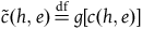 $\tilde{c}(h, e) \mathop = \limits^{{\rm{df}}} g[c(h, e)]$
, as a function of h, is a probability function.
$\tilde{c}(h, e) \mathop = \limits^{{\rm{df}}} g[c(h, e)]$
, as a function of h, is a probability function.
This theorem is a considerable generalization of proposition 1, which stated that the weighted arithmetic mean gives rise to the probability calculus. If the function f is a linear function (defining the arithmetic mean), then the probability transform g is the identity. All other f-means defined on the unit interval produce nonprobabilistic degrees of confirmation, which, however, can be transformed to probabilities. Hence, if truth-value aggregation is explicated by any generalized f-mean, probabilities can still be chosen to represent degrees of confirmation.
Proposition 1 had an important addendum: If the weights chosen for the arithmetic mean attributed to the outcomes are constant (that is, independent of e), then degrees of confirmation c(h, e) are conditional probabilities of the hypotheses h on the evidence e (see proposition 2). I shall next establish an analogous result for the generalized f-mean.
Beforehand, I have to explain what conditioning means in the generalized case. Since degrees of confirmation given by truth-value aggregation with some f-mean are, in general, not even probabilities, they cannot be conditional probabilities either. Nonetheless, there are two natural ways of defining conditioning for them; both will turn out to be equivalent.
The first is to use standard conditioning for the transformed degrees of confirmation (which are probabilities by virtue of theorem 2) and to transform them back using the inverse of the probability transform. So with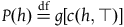 $P(h) \mathop = \limits^{{\rm{df}}} g[c(h, \top)]$
being the probability function corresponding to the prior degrees of confirmation, we say that c(h, e) satisfies generalized conditioning if
$P(h) \mathop = \limits^{{\rm{df}}} g[c(h, \top)]$
being the probability function corresponding to the prior degrees of confirmation, we say that c(h, e) satisfies generalized conditioning if $c(h, e) = g^{-1}[P(h \mid e)]$
.
$c(h, e) = g^{-1}[P(h \mid e)]$
.
The second idea is to generalize the observation made in section 3 to the effect that standard conditionalization is itself a weighted arithmetic mean of truth-values; namely, $P(h \mid e) = M^\mathrm{ari}_{\langle P(h \land e), P(\overline{h} \land e) \rangle}(1, 0)$
. Likewise, we may say that generalized conditioning should be a weighted f-mean of truth-values: c(h, e) is said to respect generalized conditioning if
$P(h \mid e) = M^\mathrm{ari}_{\langle P(h \land e), P(\overline{h} \land e) \rangle}(1, 0)$
. Likewise, we may say that generalized conditioning should be a weighted f-mean of truth-values: c(h, e) is said to respect generalized conditioning if $c(h, e) = M^f_{\langle g[c(h \land e, \top)], g[c(\overline{h} \land e, \top)] \rangle} (1, 0)$
. Here, the probability transform has been used in the weights because weights are additive. The following result, shown in the appendix, states that the two ideas coincide.
$c(h, e) = M^f_{\langle g[c(h \land e, \top)], g[c(\overline{h} \land e, \top)] \rangle} (1, 0)$
. Here, the probability transform has been used in the weights because weights are additive. The following result, shown in the appendix, states that the two ideas coincide.
Proposition 4 (generalized conditioning). Both ways of defining generalized conditioning for degrees of confirmation relative to a generalized f-mean are equivalent.
If the weights used in the generalized f-mean are attributed directly to the outcomes and held constant irrespective of the evidence, the resulting degrees of confirmation are guaranteed to fall in line with generalized conditioning. This important corollary to theorem 2 is demonstrated in the appendix.
Corollary 1 (generalized conditioning from constant weights). If for all admissible e, the aggregation function is a weighted generalized f-mean with weights assigned to the outcomes in $\Omega$
(independently of e), then the resulting degrees of confirmation satisfy generalized conditioning.
$\Omega$
(independently of e), then the resulting degrees of confirmation satisfy generalized conditioning.
When nonprobabilistic degrees of confirmation respect generalized conditioning, we can employ standard conditional probabilities to do all the calculations. At any stage, the nonprobabilistic degrees of confirmation are retained by applying the inverse of the probability transform. In this sense, conditional probabilities may be chosen by convention to represent degrees of confirmation.
There are two important qualifications. First, the mathematical correspondence between nonprobabilistic and probabilistic degrees of confirmation does not guarantee their equivalence in other ways. Different calculi may be motivated philosophically, for example, by different interpretations of degrees of confirmation or different background assumptions or facts. Mathematically, they vary in how they quantify differences in confirmation; only ordinal comparisons of degrees of confirmation are invariant under the probability transform.Footnote 25 That said, pursuing these considerations would lead outside the scope of this work, which has tried to steer clear of specific interpretations of degrees of confirmation and theories of induction.
Second, although the generalized f-means form a large class of prima facie plausible aggregation methods, they remain limited in important ways. For instance, they do not provide any advantage over standard probabilities in the treatment of fair infinite lotteries. The calculus introduced in section 4 is incompatible with any f-mean. So while (conditional) probabilities can be used widely to represent degrees of confirmation, they arguably cannot be employed universally.
6. Conclusion
This work has put forward a formal framework for degrees of confirmation that does not presuppose probabilities or any other particular calculus; its fundamental desiderata or axioms do not anticipate algebraic operations like addition (as in the additivity of probabilities) or multiplication (as in the multiplication rule for conditional probabilities). In this framework, degrees of confirmation are the result of what I have called truth-value aggregation. The possible truth-values of a hypothesis given the evidence are aggregated into a joint evaluation: its degree of confirmation.
Truth-value aggregation is comparable to a mathematical mean or average of truth-values. If it is spelled out by the standard weighted arithmetic mean, degrees of confirmation become probabilities; if the weights are always held constant, degrees of confirmation satisfy Bayesian conditionalization.
For a large and well-known class of alternative mathematical means—the weighted generalized f-means—degrees of confirmation obtained via truth-value aggregation generally cease to be probabilities. Yet they allow for a probability transform and hence for a probabilistic representation, underscoring the wide applicability of probabilities.
Wide applicability, however, does not equal universal applicability. Fair infinite lotteries, for example, fundamentally defy the standard calculus of probabilities. This is not merely a philosophical footnote, because fair infinite lotteries are reminiscent of the measure problem in early-universe cosmology (Smeenk Reference Smeenk2014). In the general formalism of truth-value aggregation, they give rise to an inherently nonprobabilistic calculus, equivalent to Norton’s (Reference Norton2021a) “infinite lottery inductive logic.” The general framework developed in this work thus not only helps to situate and to support but also to delimit the role of probabilities in confirmation theory.
Acknowledgments
I am very grateful to Anouk Barberousse, Igor Douven, Isabelle Drouet, Sarah Reboullet, and Jon Williamson for inspiring discussions and comments. I would also like to thank two anonymous reviewers for helpful and valuable suggestions.
Funding Information
None to declare.
Declarations
None to declare.
Appendix A. Mathematical proofs
Proof of theorem 1. “ $\Rightarrow$
”. Let c be a confirmation function on
$\Rightarrow$
”. Let c be a confirmation function on $\mathcal{F}$
that satisfies all the desiderata. By intensionality, c(h, e)—for admissible e and as a function of h—only depends on the valuation
$\mathcal{F}$
that satisfies all the desiderata. By intensionality, c(h, e)—for admissible e and as a function of h—only depends on the valuation $\unicode{x27E6}h\unicode{x27E7}$
, and by monotonicity, this dependence reduces to the restricted valuation
$\unicode{x27E6}h\unicode{x27E7}$
, and by monotonicity, this dependence reduces to the restricted valuation $\unicode{x27E6}h\unicode{x27E7}_e$
(see also footnote 4). So we may write
$\unicode{x27E6}h\unicode{x27E7}_e$
(see also footnote 4). So we may write $c(h, e) = m_e(\unicode{x27E6}h\unicode{x27E7}_e)$
. The codomain X is partially ordered by c
omparability, and it contains the minimal and maximal elements conventionally labeled
$c(h, e) = m_e(\unicode{x27E6}h\unicode{x27E7}_e)$
. The codomain X is partially ordered by c
omparability, and it contains the minimal and maximal elements conventionally labeled $\mathbf{\bf 0}$
and
$\mathbf{\bf 0}$
and $\mathbf{\bf 1}$
by virtue of
logicality, which also implies (1). Finally, (2) is a direct consequence of m
onotonicity.
$\mathbf{\bf 1}$
by virtue of
logicality, which also implies (1). Finally, (2) is a direct consequence of m
onotonicity.
“ $\Leftarrow$
”. Let
$\Leftarrow$
”. Let $c(h, e) = m_e(\unicode{x27E6}h\unicode{x27E7}_e)$
for all admissible e and
$c(h, e) = m_e(\unicode{x27E6}h\unicode{x27E7}_e)$
for all admissible e and $h \in \mathcal{F}$
such that
$h \in \mathcal{F}$
such that $m_e : \unicode{x27E6}\mathcal{F}\unicode{x27E7}_e \to X$
, with a partially ordered set X, satisfies (1) and (2). Intensionality concerning h is guaranteed because
$m_e : \unicode{x27E6}\mathcal{F}\unicode{x27E7}_e \to X$
, with a partially ordered set X, satisfies (1) and (2). Intensionality concerning h is guaranteed because $m_e$
only depends on the valuation of h. Concerning e, intensionality follows from the choice to represent propositions as subsets because logically equivalent propositions e, e′ are equal qua subsets, and hence
$m_e$
only depends on the valuation of h. Concerning e, intensionality follows from the choice to represent propositions as subsets because logically equivalent propositions e, e′ are equal qua subsets, and hence $m_e = m_{e'}$
. (Had we chosen to represent propositions differently, we would have had to demand, in addition, that
$m_e = m_{e'}$
. (Had we chosen to represent propositions differently, we would have had to demand, in addition, that $m_e$
only depends on e’s truth-conditional content.) Logicality follows from (1). The partial order relation in comparability is inherited from the partial order on the codomain X; the (unique) minimality of the value
$m_e$
only depends on e’s truth-conditional content.) Logicality follows from (1). The partial order relation in comparability is inherited from the partial order on the codomain X; the (unique) minimality of the value ${\bf 0}$
and the (unique) maximality of the value
${\bf 0}$
and the (unique) maximality of the value ${\bf 1}$
follow from (1) and (2). Finally, m
onotonicity holds as a result of (2).□
${\bf 1}$
follow from (1) and (2). Finally, m
onotonicity holds as a result of (2).□
Proof of proposition 1. The gist of the proof is that calculating degrees of confirmation by a weighted arithmetic mean is formally equivalent to calculating a probability measure from a probability mass function. In the finite case, without loss of generality, $e = \{\omega_1, \ldots, \omega_n\}$
and
$e = \{\omega_1, \ldots, \omega_n\}$
and $\Omega = \{\omega_1, \ldots, \omega_{n+k}\}$
with
$\Omega = \{\omega_1, \ldots, \omega_{n+k}\}$
with $k \geq 0$
. The normalized weights of the weighted arithmetic mean act as a probability mass function
$k \geq 0$
. The normalized weights of the weighted arithmetic mean act as a probability mass function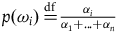 $p({\omega _i})\mathop = \limits^{{\rm{df}}} {{{\alpha _i}} \over {{\alpha _1} + \ldots + {\alpha _n}}}$
on
$p({\omega _i})\mathop = \limits^{{\rm{df}}} {{{\alpha _i}} \over {{\alpha _1} + \ldots + {\alpha _n}}}$
on $e \subseteq \Omega$
(i.e., for
$e \subseteq \Omega$
(i.e., for $1 \leq i \leq n$
), which can be extended to all of
$1 \leq i \leq n$
), which can be extended to all of $\Omega$
by setting
$\Omega$
by setting $p(\omega_{n+j}) \mathop = \limits^{{\rm{df}}} 0$
for all
$p(\omega_{n+j}) \mathop = \limits^{{\rm{df}}} 0$
for all $1 \leq j \leq k$
. Now
$1 \leq j \leq k$
. Now $c(h,e) = {{\sum\nolimits_{i = 1}^n {{\alpha _i}} {{\unicode{x27E6}h\unicode{x27E7}}^{{\omega _i}}}} \over {\sum\nolimits_{i = 1}^n {{\alpha _i}} }} = \sum\nolimits_{\omega \in h \wedge e} p (\omega ) = \sum\nolimits_{\omega \in h} p (\omega )$
, where the last step uses
$c(h,e) = {{\sum\nolimits_{i = 1}^n {{\alpha _i}} {{\unicode{x27E6}h\unicode{x27E7}}^{{\omega _i}}}} \over {\sum\nolimits_{i = 1}^n {{\alpha _i}} }} = \sum\nolimits_{\omega \in h \wedge e} p (\omega ) = \sum\nolimits_{\omega \in h} p (\omega )$
, where the last step uses $p(\omega) = 0$
for
$p(\omega) = 0$
for $\omega \in \Omega \setminus e$
. Degrees of confirmation c(h, e) thus satisfy the probability axioms as a function of h by virtue of being constructed in the standard way from a probability mass function.
$\omega \in \Omega \setminus e$
. Degrees of confirmation c(h, e) thus satisfy the probability axioms as a function of h by virtue of being constructed in the standard way from a probability mass function.
In the infinite case, the normalized weights are replaced by a normalized measure $\alpha$
on an algebra
$\alpha$
on an algebra $\mathcal{F}_e$
over e (see also footnote 9). It is extended to a normalized measure
$\mathcal{F}_e$
over e (see also footnote 9). It is extended to a normalized measure $\tilde\alpha$
on the full algebra
$\tilde\alpha$
on the full algebra $\mathcal{F}$
by defining
$\mathcal{F}$
by defining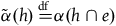 $\tilde\alpha(h) \mathop = \limits^{{\rm{df}}} \alpha(h \cap e)$
. Then
$\tilde\alpha(h) \mathop = \limits^{{\rm{df}}} \alpha(h \cap e)$
. Then $c(h, e) = \alpha(h \cap e) = \tilde\alpha(h)$
. Normalized measures are formally the same as probability measures. Note that the existence of a measure presupposes that the propositions form a
$c(h, e) = \alpha(h \cap e) = \tilde\alpha(h)$
. Normalized measures are formally the same as probability measures. Note that the existence of a measure presupposes that the propositions form a $\sigma$
-algebra: an algebra closed under countable (not only finite) disjunctions and conjunctions. This could be avoided by moving to finitely additive measures, leading to merely finitely additive probability functions.□
$\sigma$
-algebra: an algebra closed under countable (not only finite) disjunctions and conjunctions. This could be avoided by moving to finitely additive measures, leading to merely finitely additive probability functions.□
Proof of proposition 3. “ $\Leftarrow$
”. If
$\Leftarrow$
”. If $|h \cap e| = |h' \cap e|$
and
$|h \cap e| = |h' \cap e|$
and $|\overline{h} \cap e| = |\overline{h'} \cap e|$
, there are two bijections
$|\overline{h} \cap e| = |\overline{h'} \cap e|$
, there are two bijections $\pi_1 : h \cap e \to h' \cap e$
and
$\pi_1 : h \cap e \to h' \cap e$
and $\pi_2 : \overline{h} \cap e \to \overline{h'} \cap e$
. They combine to a bijection
$\pi_2 : \overline{h} \cap e \to \overline{h'} \cap e$
. They combine to a bijection $\pi_e$
on e that can be completed by the identity on
$\pi_e$
on e that can be completed by the identity on $\Omega \setminus e$
to a permutation
$\Omega \setminus e$
to a permutation $\pi$
on
$\pi$
on $\Omega$
with
$\Omega$
with $\pi(h) = h'$
and
$\pi(h) = h'$
and $\pi(e) = e$
. So label independence entails
$\pi(e) = e$
. So label independence entails $c(h, e) = c(\pi(h), \pi(e)) = c(h', e)$
.
$c(h, e) = c(\pi(h), \pi(e)) = c(h', e)$
.
“ $\Rightarrow$
”. We assume that label independence entails
$\Rightarrow$
”. We assume that label independence entails $c(h, e) = c(h', e)$
. Then there is a permutation
$c(h, e) = c(h', e)$
. Then there is a permutation $\pi : \Omega \to \Omega$
whose restriction on e defines a bijection
$\pi : \Omega \to \Omega$
whose restriction on e defines a bijection $\pi_e : e \to e$
with
$\pi_e : e \to e$
with $\pi_e(h \cap e) = h' \cap e$
. Then also
$\pi_e(h \cap e) = h' \cap e$
. Then also $\pi_e(\overline{h} \cap e) = \overline{h'} \cap e$
because
$\pi_e(\overline{h} \cap e) = \overline{h'} \cap e$
because $\pi_e$
is onto. Two sets related by a bijection have equal cardinality, so
$\pi_e$
is onto. Two sets related by a bijection have equal cardinality, so $|h \cap e| = |h' \cap e|$
and
$|h \cap e| = |h' \cap e|$
and $|\overline{h} \cap e| = |\overline{h'} \cap e|$
.□
$|\overline{h} \cap e| = |\overline{h'} \cap e|$
.□
Proof of theorem 2. Define $g : [0, 1] \to [0, 1]$
,
$g : [0, 1] \to [0, 1]$
,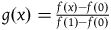 $g(x) = {{f(x) - f(0)} \over {f(1) - f(0)}}$
. Since g is a linear transform of f, it is easy to see and well known that the g-mean always equals the f-mean,
$g(x) = {{f(x) - f(0)} \over {f(1) - f(0)}}$
. Since g is a linear transform of f, it is easy to see and well known that the g-mean always equals the f-mean, $M^g_\alpha = M^f_\alpha$
(see, e.g., Bullen Reference Bullen2003, 271). Also,
$M^g_\alpha = M^f_\alpha$
(see, e.g., Bullen Reference Bullen2003, 271). Also, $g(0) = 0$
and
$g(0) = 0$
and $g(1) = 1$
: Truth-values are fixed points of g. Without loss of generality, assume that the weights are normalized. In the finite case, let
$g(1) = 1$
: Truth-values are fixed points of g. Without loss of generality, assume that the weights are normalized. In the finite case, let $e = \{ \omega_1, \ldots, \omega_n \}$
,
$e = \{ \omega_1, \ldots, \omega_n \}$
, $n \geq 1$
, without loss of generality. Then
$n \geq 1$
, without loss of generality. Then $c(h, e) = M^f_\alpha(\unicode{x27E6}h\unicode{x27E7}^{\omega_1}, \ldots, \unicode{x27E6}h\unicode{x27E7}^{\omega_n}) = M^g_\alpha(\unicode{x27E6}h\unicode{x27E7}^{\omega_1}, \ldots, \unicode{x27E6}h\unicode{x27E7}^{\omega_n}) = g^{-1}\!\left( \sum_{i=1}^{n} \alpha_i g(\unicode{x27E6}h\unicode{x27E7}^{\omega_i} \right) = g^{-1}\!\left( \sum_{i=1}^{n} \alpha_i \,\unicode{x27E6}h\unicode{x27E7}^{\omega_i} \right)$
. So
$c(h, e) = M^f_\alpha(\unicode{x27E6}h\unicode{x27E7}^{\omega_1}, \ldots, \unicode{x27E6}h\unicode{x27E7}^{\omega_n}) = M^g_\alpha(\unicode{x27E6}h\unicode{x27E7}^{\omega_1}, \ldots, \unicode{x27E6}h\unicode{x27E7}^{\omega_n}) = g^{-1}\!\left( \sum_{i=1}^{n} \alpha_i g(\unicode{x27E6}h\unicode{x27E7}^{\omega_i} \right) = g^{-1}\!\left( \sum_{i=1}^{n} \alpha_i \,\unicode{x27E6}h\unicode{x27E7}^{\omega_i} \right)$
. So $g[c(h, e)] = \sum_{i=1}^{n} \alpha_i \,\unicode{x27E6}h\unicode{x27E7}^{\omega_i}$
, which is the weighted arithmetic mean
$g[c(h, e)] = \sum_{i=1}^{n} \alpha_i \,\unicode{x27E6}h\unicode{x27E7}^{\omega_i}$
, which is the weighted arithmetic mean $M^{\rm ari}_\alpha(\unicode{x27E6}h\unicode{x27E7}^{\omega_1}, \ldots, \unicode{x27E6}h\unicode{x27E7}^{\omega_n})$
and thus a probability function by proposition 1. In the infinite case with a normalized measure (see also footnote 5), we likewise have
$M^{\rm ari}_\alpha(\unicode{x27E6}h\unicode{x27E7}^{\omega_1}, \ldots, \unicode{x27E6}h\unicode{x27E7}^{\omega_n})$
and thus a probability function by proposition 1. In the infinite case with a normalized measure (see also footnote 5), we likewise have $c(h, e) = M^f_\alpha(\unicode{x27E6}h\unicode{x27E7}_e) = M^g_\alpha(\unicode{x27E6}h\unicode{x27E7}_e) = g^{-1}\!\left( \int_{e} g \circ \unicode{x27E6}h\unicode{x27E7}_e \,{\rm d}\alpha \right) = g^{-1}\!\left( \int_{e} \,\unicode{x27E6}h\unicode{x27E7}_e \,{\rm d}\alpha \right)$
, and hence
$c(h, e) = M^f_\alpha(\unicode{x27E6}h\unicode{x27E7}_e) = M^g_\alpha(\unicode{x27E6}h\unicode{x27E7}_e) = g^{-1}\!\left( \int_{e} g \circ \unicode{x27E6}h\unicode{x27E7}_e \,{\rm d}\alpha \right) = g^{-1}\!\left( \int_{e} \,\unicode{x27E6}h\unicode{x27E7}_e \,{\rm d}\alpha \right)$
, and hence $g\left[ M^f_\alpha(\unicode{x27E6}h\unicode{x27E7}_e)\right] = \int_{e} \,\unicode{x27E6}h\unicode{x27E7}_e \,{\rm d}\alpha = M^{\rm ari}_\alpha(\unicode{x27E6}h\unicode{x27E7}_e)$
.□
$g\left[ M^f_\alpha(\unicode{x27E6}h\unicode{x27E7}_e)\right] = \int_{e} \,\unicode{x27E6}h\unicode{x27E7}_e \,{\rm d}\alpha = M^{\rm ari}_\alpha(\unicode{x27E6}h\unicode{x27E7}_e)$
.□
Proof of proposition 4. Starting from the second definition, we use that for arbitrary weights, $M^f_{\langle \alpha_1, \alpha_2 \rangle}(1, 0) = M^g_{\langle \alpha_1, \alpha_2 \rangle}(1, 0)$
(see the proof of theorem 2). So
$M^f_{\langle \alpha_1, \alpha_2 \rangle}(1, 0) = M^g_{\langle \alpha_1, \alpha_2 \rangle}(1, 0)$
(see the proof of theorem 2). So $M_{\langle g[c(h \wedge e, \top )],g[c(\bar h \wedge e, \top )]\rangle }^f(1,0)=$ ${g^{ - 1}}\left[ {{{g[c(h \wedge e, \top )] \cdot 1 + g[c(\bar h \wedge e, \top )] \cdot 0} \over {g[c(h \wedge e, \top )] + g[c(\bar h \wedge e, \top )]}}} \right] = {g^{ - 1}}\left[ {{{g[c(h \wedge e, \top )]} \over {g[c(e, \top )]}}} \right] = {g^{ - 1}}\left[ {{{P(h \wedge e)} \over {P(e)}}} \right] = {g^{ - 1}}[P(h\mid e)]$
. This equals the first definition. □
${g^{ - 1}}\left[ {{{g[c(h \wedge e, \top )] \cdot 1 + g[c(\bar h \wedge e, \top )] \cdot 0} \over {g[c(h \wedge e, \top )] + g[c(\bar h \wedge e, \top )]}}} \right] = {g^{ - 1}}\left[ {{{g[c(h \wedge e, \top )]} \over {g[c(e, \top )]}}} \right] = {g^{ - 1}}\left[ {{{P(h \wedge e)} \over {P(e)}}} \right] = {g^{ - 1}}[P(h\mid e)]$
. This equals the first definition. □
Proof of corollary 1. In the finite case, assume $e = \{\omega_1, \ldots, \omega_k\}$
and
$e = \{\omega_1, \ldots, \omega_k\}$
and $\Omega = \{\omega_1, \ldots, \omega_n\}$
with
$\Omega = \{\omega_1, \ldots, \omega_n\}$
with $1 \leq k \lt n$
without loss of generality. I shall use that the generalized f-mean equals the generalized g-mean, where g is the probability transform, and that truth-values are fixed points of g—that is,
$1 \leq k \lt n$
without loss of generality. I shall use that the generalized f-mean equals the generalized g-mean, where g is the probability transform, and that truth-values are fixed points of g—that is, $g(0) = 0$
and
$g(0) = 0$
and $g(1) = 1$
(see the proof of theorem 2). Then by truth-value aggregation for any h out of the algebra,
$g(1) = 1$
(see the proof of theorem 2). Then by truth-value aggregation for any h out of the algebra, $c(h,e) = M_\alpha ^f\left( {{{\unicode{x27E6}h\unicode{x27E7}}^{{\omega _1}}}, \ldots, {{\unicode{x27E6}h\unicode{x27E7}}^{{\omega _k}}}} \right) = {g^{ - 1}}\left[ {{{\sum\nolimits_{i = 1}^k {{\alpha _i}} g({{\unicode{x27E6}h\unicode{x27E7}}^{{\omega _i}}})} \over {\sum\nolimits_{i = 1}^k {{\alpha _i}} }}} \right] = {g^{ - 1}}\left[ {{{\sum\nolimits_{i = 1}^k {{\alpha _i}} {\mkern 1mu} {{\unicode{x27E6}h\unicode{x27E7}}^{{\omega _i}}}} \over {\sum\nolimits_{i = 1}^k {{\alpha _i}} }}} \right] = {g^{ - 1}}[P(h\mid e)]$
, where I have identified the weighted arithmetic mean in the argument with a conditional probability by virtue of proposition 2. The infinite case is completely analogous; sums are replaced by corresponding integrals. □
$c(h,e) = M_\alpha ^f\left( {{{\unicode{x27E6}h\unicode{x27E7}}^{{\omega _1}}}, \ldots, {{\unicode{x27E6}h\unicode{x27E7}}^{{\omega _k}}}} \right) = {g^{ - 1}}\left[ {{{\sum\nolimits_{i = 1}^k {{\alpha _i}} g({{\unicode{x27E6}h\unicode{x27E7}}^{{\omega _i}}})} \over {\sum\nolimits_{i = 1}^k {{\alpha _i}} }}} \right] = {g^{ - 1}}\left[ {{{\sum\nolimits_{i = 1}^k {{\alpha _i}} {\mkern 1mu} {{\unicode{x27E6}h\unicode{x27E7}}^{{\omega _i}}}} \over {\sum\nolimits_{i = 1}^k {{\alpha _i}} }}} \right] = {g^{ - 1}}[P(h\mid e)]$
, where I have identified the weighted arithmetic mean in the argument with a conditional probability by virtue of proposition 2. The infinite case is completely analogous; sums are replaced by corresponding integrals. □





































 Open access

