A) Collection protocol

In order to develop a technique for quantifying the cognitive state/stress level of drivers, driving data are recorded under various driving conditions with four different secondary tasks. Detailed descriptions of the tasks and examples of the spoken sentences are follow as:

• • Signboard reading task: Drivers read aloud words on signboards, such as names of shops and restaurants, seen from the driver seat while driving, e.g., “7–11”, “Dennys”.

• • Navigation dialog task: Drivers are guided to an unfamiliar location by a navigator via a cell phone with a hands-free headset. Drivers do not have maps, and only the navigator knows the route to the destination.

• • Alphanumeric reading task: Drivers repeat random four-character strings consisting of the letters a–z and digits 0–9, e.g., “UKZ5”, “IHD3”, “BJB8”. The original four-character strings are supplied through an earphone.

• • Music retrieval task: Drivers retrieve and play music using a spoken dialog interface. Music can be retrieved by the artist's name or the song title, e.g., “Beatles”, “Yesterday”.

Drivers start from Nagoya University and return after about 70 min of driving. Driving data are recorded under the above four task conditions on city roads, and under two task conditions on an expressway. Driving data without any tasks are recorded as a reference before, between, and after the tasks. Figure 3 shows some samples of driving signals.

Fig. 3.

Examples of driving behavior signals.

After completing the route, the participant is asked to assess his or her subjective level of frustration while driving, by simultaneously viewing the front-view camera and facial videos while listening to the corresponding audio recording. The assessment is done on a custom designed computer interface, on which the driver continuously indicates the intensity of their frustration by sliding a bar along a scale from 0 to 30, i.e., from “no frustration” to “extremely frustrated”. The interface output is a continuous signal, and the level of frustration is recorded every 0.1 s.

B) Data annotation

An effective annotation of the collected multimedia information is crucial for providing a more meaningful description of the situations drivers experience. In our study, we proposed a data annotation protocol that covers most of the factors that might affect drivers and influence their subjective feedback responses. The annotation labels are comprised of six major groups: driver's affective state (level of irritation), driver actions (e.g., facial expression), driver's secondary task, driving environment (e.g., type of road, traffic density), vehicle status (e.g., turning, stopped), and speech/background noise. The annotation protocol designed in this research is comprehensive, and can be used in a wide range of research fields. Further details of the annotation protocol and a more detailed description can be found in [Reference Malta, Angkititrakul, Miyajima and Takeda11]. Having introduced our driving corpus, in the following sections we will discuss signal processing techniques and data-driven approaches for various vehicle applications.

A) Spectral features of pedal operation signals

As shown in Fig. 5, in driver modeling we assume that the command signal for hitting a pedal e(n) is filtered with driver model H(e ^jω), represented as the spectral envelope, and that the output of the system is observed as pedal signal x(n). In other words, a command signal is generated when the driver decides to apply pressure to the gas pedal, and H(e ^jω) represents the process of acceleration. This can be described in the frequency domain as follows:

(3)$$X\lpar e^{j\omega}\rpar =E\lpar e^{j\omega}\rpar H\lpar e^{j\omega }\rpar \comma$$

where X(e ^jω) and E(e ^jω) are the Fourier transforms of x(n) and e(n), respectively. We focus on driver characteristics represented as frequency response H(e ^jω).

Fig. 5.

General modeling of a driving signal.

A cepstrum is a widely used spectral feature for speech and speaker recognition [Reference Rabiner and Juang14], defined as the inverse Fourier transform of the log power spectrum of the signal. Cepstral analysis allows us to smooth the structure of the spectrum by keeping only the first several lower-order cepstral coefficients, and setting the remaining coefficients to zero. Assuming that individual differences in pedal operation patterns can be represented by the smoothed spectral envelope of pedal operation signals, we modeled the pedal operation patterns of each driver with lower-order cepstral coefficients. In addition, assuming that the spectral envelope can capture the differences between the characteristics of different drivers, we focused on the differences in spectral envelopes represented by cepstral coefficients (cepstrum), which were also modeled with GMMs.

1) DYNAMIC FEATURES OF DRIVING SIGNALS

In a way similar to research done on speech and speaker recognition, we found that the dynamic features of driving signals contain large amounts of information about driving behavior. Dynamic features are defined as the following linear regression coefficients:

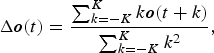(4)$$\Delta {\bi o}\lpar t\rpar ={\sum^{K}_{k=-K}k{\bi o}\lpar t+k\rpar \over \sum^{K}_{k=-K}k^2}\comma$$

where o(t) is a static feature of raw signals or cepstral coefficients at time t and K is the half window size for calculating the Δ coefficients. We determined from preliminary experiments that the regression window is 2K = 800 ms for both raw pedal signals and cepstral coefficients. If o (t) is a D-dimensional vector, D dynamic coefficients are obtained from the static coefficients, combined into a 2D-dimensional feature vector, and modeled with GMMs.

B) Driver identification experiments

1) EXPERIMENTAL CONDITIONS

Driving data from 276 drivers, collected on city roads in the data collection vehicle, were used, excluding data collected while the vehicle was not moving. Three minutes of driving signals were used for GMM training and another 3 min for testing. We used both brake and gas pedal signals in the real-vehicle experiments because drivers use the brake pedal more often during city driving than during expressway driving.

Cepstral coefficients obtained from the gas and brake pedal signals are modeled with two separated GMMs, and their log-likelihood scores were linearly combined. For driver identification, the unknown driver was identified as driver $\hat{k}$ who gave the maximum weighted GMM log-likelihood over the gas and brake pedal signals:

(5)$$\eqalign{\hat{k}&=\arg\max_{k}\lcub \gamma\log P\lpar {\bi G}\mid\lambda_{G\comma k}\rpar \cr & \quad +\lpar 1-\gamma\rpar \log P\lpar {\bi B}\mid\lambda_{B\comma k}\rpar \rcub \comma \; \quad 0\leq \gamma \leq 1\comma}$$

where G and B are the cepstral sequences of the gas and brake pedals and λ_{G, k} and λ_{B, k} are the kth driver models of the gas and brake pedals, respectively. γ is a linear combination weight for the log-likelihood of gas pedal signals.

2) EXPERIMENTAL RESULTS

The results for the 16-component GMMs are summarized in Fig. 6. The identification performance was rather low when using raw driving signals: the best identification rate for raw signals was 47.5% with γ = 0.80. By applying cepstral analysis, however, the identification rate increased to 76.8% with γ = 0.76. We thus conclude that cepstral features capture individual variations in driving behavior better than raw driving signals and achieve better performance in driver identification.

Fig. 6.

Comparison of identification rates using raw pedal signals and cepstral coefficients.

A) Car following

Car following characterizes longitudinal behavior of a driver while following behind another vehicle [Reference Brackstone and McDonald18]. In this study, we focus on the way the behavior of the driver of the following vehicle is affected by the driving environment and by the states of his or her own vehicle. There are several factors that affect car-following behavior, such as relative position and velocity of following vehicle with respect to lead vehicle, acceleration and deceleration of both vehicles, and perception ability and reaction time of the follower. Figure 7 shows a basic diagram of car following and the corresponding parameters, where v _t^f, a _t^f, f _t, x_t^f represent vehicle velocity, acceleration/deceleration, distance between vehicles, and observed feature vector at time t, respectively.

Fig. 7.

Car following with corresponding parameters.

The GMM-based driver-behavior model represents patterns of pedal operation corresponding to the observed velocity and following distance. The underlying premise of this modeling framework is that a driver determines gas and brake pedal operation in response to the stimulus of vehicle velocity and following distance. Consequently, such relationship can be modeled by the joint distribution of all the correlated parameters. Figure 8 illustrates a car-following trajectory (gray dashed line) on different 2-D parameter spaces, overlaid with the contour of corresponding two-mixture GMM distribution.

Fig. 8.

A car-following trajectory (gray dashed line) on different two-dimensional parameter spaces, overlaid with the contour of corresponding two-mixture GMM distribution.

1) FEATURE EXTRACTION AND MODEL REPRESENTATION

In our framework to model a pedal pattern, an observed feature vector at time t, x_t, consists of vehicle velocity, following distance, and pedal pattern (G _t) with their first- (Δ) and second-order (Δ²) time derivatives as

(6)$${\bf x}_t = \lsqb v_t^f\comma \; \Delta v_t^f\comma \; \Delta^2 v_t^f\comma \; f_t\comma \; \Delta f_t\comma \; \Delta^2 f_t\comma \; G_t\comma \; \Delta G_t\comma \; \Delta^2 G_t\rsqb ^T\comma$$

where, in this modeling, the Δ(·) operator is defined as

(7)$$\Delta x_t = x_t - {\sum_{\tau=1}^{\open T}\tau x_{t-\tau}\over \sum_{\tau=1}^{\open T} \tau}\comma$$

where $\open T$ is a window length (e.g., 0.8 s). Next, let us define a set of augmented feature vectors y_t as

(8)$${\bf y}_t = \lsqb {\bf x}_t^T {G}_{t+1}\rsqb ^T.$$

Consequently, the joint density between the observed driving signals x_t and the next pedal operation G _t+1 can be modeled by a GMM Φ, with a mean vector μ_k^y and a covariance matrix ∑_k^yy of the kth mixture expressed as

(9)$$\mu_k^y =\left[\matrix {\mu^{\bf x}_k \cr \mu_k^G }\right]\, \hbox{and}\, {\Sigma_{k}^{yy}}=\left[\matrix{\Sigma_k^{\bf xx}\quad\Sigma_k^{{\bf x}G}\cr \Sigma_k^{G{\bf x}}\quad\Sigma_k^{GG}}\right].$$

2) PEDAL PATTERN PREDICTION

The predicted gas pedal pattern Ĝ _t+1 is computed using the weighted predictions resulting from all the mixture components of the GMM, as

(10)$${\hat G}_{t+1} = \sum_{k=1}^K h_k\lpar {\bf x}_t\rpar \cdot {\hat G}_{t+1}^{\lpar k\rpar }\lpar {\bf x}_t\rpar \comma$$

where Ĝ _t+1^(k)(x_t) is a maximum a posteriori (MAP) prediction of the observed parameters x_t given the kth mixture component which is given by

(11)$$\eqalign{{\hat G}_{t+1}^{\lpar k\rpar }\lpar {\bf x}_t\rpar &= arg\max_{G_{t+1}} \lcub p\lpar G_{t+1} \vert {\bf x}_t\comma \; \phi_k\rpar \rcub \cr & \quad =\mu_k^{G} + \Sigma_k^{{G}x}\lpar \Sigma_k^{xx}\rpar ^{-1}\lpar {\bf x}_t-\mu_k^x\rpar .}$$

The term h _k(x_t) is the posterior probability of the observed parameter x_t belonging to the kth-mixture component, as

(12)$$h_k\lpar {\bf x}_t\rpar = {\alpha_k p\lpar {\bf x}_t\vert\phi_k^x\rpar \over\sum_{i=1}^K \alpha_i p\lpar {\bf x}_t\vert\phi_i^x\rpar }\comma \; 1 \leq k \leq K\comma$$

where p(x_t|ϕ_i^x) is the marginal probability of the observed parameter x_t generated by the ith Gaussian component, and α_k is the prior probability of the kth mixture component.

4) EXPERIMENTAL EVALUATION

Evaluation is performed using approximately 300 min worth of clean and realistic car-following data from 68 drivers. Manual annotation is exploited to verify that only concrete car-following events with legitimate driving signals that last more than 10 s are considered. The prediction was performed on every sample (i.e., every 0.1 s). Figure 9 compares the prediction performance of the universal, driver-adapted, and 30 s-on-line-adapted (using 30 s of driving data) driver models with 4, 8, 16, and 32 mixtures, in terms of SDR.

Fig. 9.

Comparison of pedal prediction performance for car-following task using different driver models.

The measurement SDR is defined as follows:

(13)$$SDR = 10\log_{10} {\sum_{t=1}^T G^2\lpar t\rpar \over \sum_{t=1}^T \lpar G\lpar t\rpar -{\hat G}\lpar t\rpar \rpar ^2} \lsqb \hbox{dB}\rsqb \comma$$

where T is the length of a signal, G(t) is the actually observed signal, and Ĝ (t) is the predicted signal. From the results, we can see that the driver-adapted models showed the best performance (approximately 19 dB SDR or 11.22% normalized errors with 32-mixture GMMs).

B) Lane changing

In this section, we consider driving behavior related to control of vehicle trajectory during lane changes. Since lane change activity consists of multiple states (i.e., examining the safety of traffic environments, assessing the positions of other vehicles, moving into the next lane, and adjusting driving speed to traffic flow) [Reference Chee and Tomizuka19], a single dynamic system cannot model vehicle trajectory. In addition, the boundaries between states cannot be observed from the vehicle's trajectory.

To study lane-changing behavior, a set of vehicle movement observations were made using a driving simulator. Relative longitudinal and lateral distances from a vehicle's position when starting a lane change, x _i[n], y _i[n], and the velocity of the vehicle, $\dot{x}_{i}\lsqb n\rsqb \comma \; \dot{y}_{i}\lsqb n\rsqb $, were recorded every 160 ms. Here, i = 1, 2, 3 are the indexes for the locations of surrounding vehicles (Fig. 10), and {x₀[n], y ₀[n]} represents the position of the driver's own vehicle. The duration of lane-change activity, n = 1, 2, …, N, starts when V ₀ (the drivers own vehicle) and V ₂ are at the same longitudinal position and ends when V ₀’s lateral position reaches the local minimum as shown in Fig. 10.

Fig. 10.

Lane-change trajectory and geometric positions of surrounding vehicles.

1) MODELING TRAJECTORY USING A HMM

We used a three-state HMM [Reference Rabiner20] to describe the three different stages of a lane change: preparation, shifting, and adjusting. In the proposed model, each state is characterized by a joint distribution of eight variables:

(14)$$v = \lsqb \dot{x}_0\comma \; y_0\comma \; \Delta\dot{x}_0\comma \; \Delta\dot{y}_0\comma \; \Delta^2\dot{x}_0\comma \; \Delta^2\dot{y}_0\comma \; \dot{x}_1\comma \; \dot{x}_2\rsqb ^T.$$

Here, the Δ operator is defined as in equation (4). In general, longitudinal distance, x ₀, monotonically increases in time and cannot be modeled by an i.i.d. process. Therefore, we use longitudinal speed $\dot{x}_{0}$ as a variable to characterize the trajectory. Finally, after training the HMM using a set of recorded trajectories, the mean vector μ_j and covariance matrix Σ_j of the trajectory variable v are estimated for each state (j = 1, 2, 3). The distribution of duration N is modeled using a Gaussian distribution.

The shape of a trajectory is controlled by the HMM and the total duration of the lane change activity. When a driver performs a lane change in a shorter time, this results in a sharper trajectory. We generate a set of probable lane-change trajectories by determining state durations d _j using uniform re-sampling. Once a set of state durations is determined, we apply either the maximum likelihood HMM signal synthesis algorithm (ML method) [Reference Tokuda, Yoshimura, Masuko, Kobayashi and Kitamura21] or the sampling algorithm [Reference Rubinstein and Kroese22] to generate the most probable trajectory. Simply repeating this process will produce a set of probable vehicle trajectories which characterize a driver's typical lane-change behavior.

2) TRAJECTORY SELECTION

Although various natural driving trajectories may exist, the number of lane-change trajectories that can be realized under given traffic circumstances is limited. Furthermore, the selection criteria of the trajectory, based on the traffic context, differs among drivers (e.g., some drivers are more sensitive to the position of the leading vehicle than to those of vehicles to the side.) Therefore, we model the selection criterion of each driver with a scoring function for lane-change trajectories based on vehicular contexts, i.e., relative distances to the surrounding vehicles.

In the proposed method, a hazard map function M is defined in a stochastic domain based on the histograms of the relative positions of the surrounding vehicles r _i = [x _i − x ₀, y _i − y ₀]^t. To model sensitivity to surrounding vehicles, we calculated a covariance matrix R _i for each of three distances r _i, i = 1, 2, 3, using training data. Since the distance varies more widely at less sensitive distances, we use the quadratic form of inverse covariance matrices (R _i⁻¹) as a metric of the cognitive distance. Then we calculate the hazard map function M _i for surrounding vehicle V _i as follows:

(15)$$M_i ={1 \over 1+exp\lcub \alpha_i\lpar r_i^tR_i^{-1}r_i - \beta_i\rpar \rcub }\comma$$

where α_i is a parameter of the minimum safe distance defined so that the minimum value of cognitive distance r _i^tR _i⁻¹r _i of the training data corresponds to the lower 5% distribution values, and β_i is the mean value of r _i^tR _i⁻¹r _i.

Each hazard map M _i can be regarded as a posteriori probability of being in the safe driving condition within the range of distances Pr(safe|r_i), when the likelihood is given as an exponential quadratic form. Therefore, integrating the hazard maps for all surrounding vehicles can be done simply by interpolating three probabilities with weights λ_i into an integrated map 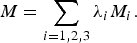$M = \sum_{i=1\comma 2\comma 3} \lambda_{i} M_{i}.$ Once the positions of the surrounding vehicles at time n, r _i[n], are determined, M _i can be calculated for each point in time, and by averaging the value over the duration of the lane change, we can compare the possible trajectories. Then the optimal trajectory that has the lowest value is selected from among the possible trajectories.

3) EXPERIMENTAL EVALUATION

Thirty lane-change trials were recorded for two drivers using a driving simulator which simulated a two-lane urban expressway with moderate traffic. The velocity of the vehicles in the passing lane ranged from 82.8 to 127.4 km/h and the distance between successive vehicles in the passing lane ranged between 85 and 315 m. The drivers were instructed to pass the lead vehicle when they were able to, once during each trial. The trained hazard maps M for the two drivers shown in Fig. 11 depicts differences in sensitivity to surrounding vehicles.

Fig. 11.

Hazard maps for two drivers when surrounding vehicles were in the same positions.

We generated possible lane-change trajectories for the vehicles over a 20-s period using the two above-mentioned methods, and then selected the optimal trajectory. Figure 12 illustrates sample trajectories generated using the sampling method and the corresponding optimal trajectory, and compares them with the actual trajectory. For quantitative evaluation, we calculated the difference between the predicted and actual trajectories based on dynamic time warping (DTW) [Reference Sakoe and Chiba23], using the normalized square difference as a local distance, and measured it in terms of signal-to-deviation ratio (SDR). Figure 13 (top) shows average SDRs of the best trajectory hypothesis and all trajectory hypotheses (mean), using the ML method (left) and the sampling method (right). The sampling method was better at generating vehicle trajectories similar to the actual driver trajectories than the ML method. Figure 13 (bottom) also shows the SDRs when driver A's model was used for predicting driver B's trajectory and vice versa. The SDR decreased by 2.2 dB when the other driver's model was used to make the prediction. This result confirmed the effectiveness of the proposed model for capturing individual characteristics of lane-change behavior. We also tested our method using actual lane-change duration. When the actual lane-change duration N is given, the root mean square error (RMSE) between the predicted and actual trajectories can be calculated. The average RMSE for 60 tests was 17.6 m, as a result of predicting vehicle trajectories over a distance of about 600 m (i.e., over a 20-s time period).

Fig. 12.

Examples of generated trajectories (black dotted lines) and optimal trajectory (blue dashed line) using sampling method, compared with actual trajectory (red solid line).

Fig. 13.

Average SDRs of lane-change trajectories. Top: the best and mean trajectories using ML method (left) versus sampling method (right). Bottom: using a driver's own model (left) versus using the other driver's model (right).

A) Analysis

A method for combining all of the different features and annotation results in an efficient language was needed, and a BN [Reference Murphy25] was the natural choice to deal with such a task. One of the important characteristics of a BN is the ability to infer the state of an unobserved variable, given the state of the observed ones. In our case, we wanted to infer a participant's frustration given the driving environment, speech recognition errors (i.e., communication environment), and the participant's responses measured through the physiological state, overall facial expression, and pedal actuation.

The graph structure proposed to integrate all of the available information is shown in Fig. 14. This model was based on the following assumptions: (1) environmental factors that may have an impact on goal-directed behavior (i.e., traffic density, stops at red-lights, obstructions, turns or curves, and speech recognition errors) may also result in driver frustration; (2) a frustrated driver is likely to exhibit changes in his or her facial expression, physiological state, and gas- and brake-pedal actuation behavior. In Fig. 14, the squares represent discrete (tabular) nodes and the circle represents a continuous (Gaussian) node. The number inside each node represents the number of mutually exclusive states that the node can assume (e.g., “2” for yes/no binary states, “4” for four levels of arousal). Random variables were identified by a label outside each node: “F” (frustration), “E” (environment), and “R” (responses).

Fig. 14.

Proposed BN structure. Squares represent discrete (tabular) nodes, and the circle represents a continuous (Gaussian) mode. The number inside each node represents the number of mutually exclusive states the node can assume. Labels outside nodes identify random variable type.

In addition to the graph structure, it is also necessary to specify the parameters of the model, obtained here using a training set. During parameterization, we calculate the conditional probability distribution (CPD) at each node. If the variables are discrete, this can be represented as a table (CPT), which lists the probability of a child node taking on each of its different values for each combination of the values of its parent nodes. On the other hand, if the variable is continuous, the CPD is assumed to have a linear-Gaussian distribution. For example, the continuous node pedal actuation, which has only one binary parent, was represented by two different multivariate Gaussians, one for each emotional state: frustrated and not frustrated. For each observed environment (driving and communication) and the corresponding driver responses, we can use Bayes’ rule to compute the posterior probability of frustration as

(16)$$\eqalign{& P\lpar F \vert E_1\comma \; E_2\comma \; E_3\comma \; E_4\comma \; E_5\comma \; R_1\comma \; R_2\comma \; R_3\comma \; R_4\rpar \cr & \quad =P\lpar F \vert E_1\comma \; E_2\comma \; E_3\comma \; E_4\comma \; E_5\rpar \cr & \quad \quad \times\displaystyle{{P\lpar R_1 \vert F\rpar P\lpar R_2 \vert F\rpar P\lpar R_3 \vert F\rpar P\lpar R_4 \vert F\rpar } \over {P\lpar E_1\comma \; E_2\comma \; E_3\comma \; E_4\comma \; E_5\comma \; R_1\comma \; R_2\comma \; R_3\comma \; R_4\rpar }}}$$

The denominator was calculated by summing (marginalizing) out F. In addition, in this study we set a uniform Dirichlet prior [Reference Ferguson26] to every discrete node in the network. This was done in order to avoid over-fitted results due to the ML approach used for calculating the CPTs. Without a priori, patterns that were not observed in the training set would be assigned zero probability, compromising the estimation.

The network input data are all of the available data–pedal actuation signals, skin potential, and other binary signals (environmental factors and speech recognition errors). At a given time step t, frames of sizes L and M were used to extract features from the skin potential and pedal actuation signals, respectively. The results served as the network inputs. The value of each binary label at the current time step was directly entered into the network without further processing. Frame shift was kept fixed at 0.5 s. For two consecutive frames, the value of current traffic density continues to remain in effect, for example, on future skin potential and pedal actuation signals, in order to account for delayed physiological and behavioral reactions. In addition, frustration was estimated for every frame (i.e., we did not pre-select segments where we were certain of the presence or absence of frustration, while ignoring ambiguous regions.)

B) Experimental evaluation

Within the data used in our experiments, 129 scenes of frustration (segments with an original value above 0) were found. On average, participants became frustrated 6.5 times while driving in our experiment. The mean strength of frustration scenes was 10.5, and the mean duration was 11.8 s. Figure 15 shows the estimation results for all drivers concatenated side by side: actual frustration detected for all 20 participants (top); the posterior probability of the frustration node calculated using the entire network (center); and the quantized posterior probability using a threshold of 0.5 (bottom). The quantized probability for each driver was further median-filtered to remove unwanted spikes. The overall results show that the model achieved a TP rate of 80% with a FP rate of 9% (i.e., the system correctly estimate 80% of the frustration and, when drivers were not frustrated, mistakenly detected frustration 9% of the time).

Fig. 15.

Results for individual drivers (arranged side by side) calculated using the entire network. Comparison between actual frustration detected for all drivers (top), posterior probability of the frustration node (center), and its quantized version using a threshold of 0.5 (bottom).

A) Experimental evaluation

In order to validate the effectiveness of our system in reducing the number of detected hazardous situations (e.g., to improve driving behavior), we recruited 33 drivers, including 6 expert drivers, to participate in our experiment. The subjects were asked to drive the instrumented vehicle three times on three different days, following the same route, which takes approximately 90 min to complete. We used data from the second and the third sessions for our analysis, because we allowed the subjects to get familiar with the vehicle during the first session. After the second session, 27 subjects used the driving diagnosis browser and received feedback before taking part in the third session. We compared the number of hazardous situations detected during the second and third sessions. Figure 18 compares the number of detected hazardous situations. We can see that the number of detected hazardous scenes for the non-expert drivers decreased by more than 50% after using the system, while there was no significant change for the drivers who did not use the system.

Fig. 18.

Number of detected hazardous scenes for non-expert drivers who did not receive feedback (top), and for non-expert and expert drivers before and after using the system (bottom).