





1. Introduction
Markov chain Monte Carlo (MCMC) algorithms, and in particular the Hamiltonian Monte Carlo (HMC) algorithms, are workhorses in many scientific fields including physics [Reference Duane, Kennedy, Pendleton and Roweth20], statistics and machine learning [Reference Andrieu, de Freitas, Doucet and Jordan2, Reference Girolami and Calderhead22, Reference Hoffman and Gelman28, Reference Mangoubi and Vishnoi41, Reference Welling and Teh60], and molecular biology [Reference Christensen, Linnet, Borg, Boomsma, Lindorff-Larsen, Hamelryck and Jense1]. An important question practitioners face is how to choose an algorithm for a particular problem. Are there any general principles that allow users to prefer one algorithm to another for generic but simple problems? One of the most fruitful branches of MCMC theory has focused on analyzing MCMC algorithms by studying their scaling limits.
One natural idea is to study how an MCMC algorithm’s speed depends on some underlying parameter, such as the dimension d of the target distribution. Results from the theory of scaling limits [Reference Beskos, Pillai, Roberts, Sanz-Serna and Stuart4], as well as non-asymptotic bounds [Reference Chen and Gatmiry18], suggest that HMC often has a running time of $O(d^{0.25})$
. This is in contrast to the random-walk metropolis (RWM) algorithm, which has a much longer running time of O(d) steps under very broad conditions [Reference Bédard3, Reference Mattingly, Pillai and Stuart43, Reference Roberts, Gelman and Gilks50]. These results and other evidence, both empirical and theoretical (see, e.g., [Reference Betancourt6, Reference Bou-Rabee, Eberle and Zimmer12, Reference Chen, Dwivedi, Wainwright and Yu17, Reference Lee, Shen and Tian31, Reference Mangoubi and Smith37, Reference Mangoubi and Smith39]) have lead to the widespread understanding that HMC is superior to RWM for a variety of problems, especially those that are high-dimensional and essentially unimodal. In this paper, we investigate the extent to which this superiority holds in another natural scaling regime: ‘highly multimodal’ target distributions that have several well-defined and well-separated modes. There is no a priori reason to believe that algorithms superior in one of these regimes are also superior in the other.
$O(d^{0.25})$
. This is in contrast to the random-walk metropolis (RWM) algorithm, which has a much longer running time of O(d) steps under very broad conditions [Reference Bédard3, Reference Mattingly, Pillai and Stuart43, Reference Roberts, Gelman and Gilks50]. These results and other evidence, both empirical and theoretical (see, e.g., [Reference Betancourt6, Reference Bou-Rabee, Eberle and Zimmer12, Reference Chen, Dwivedi, Wainwright and Yu17, Reference Lee, Shen and Tian31, Reference Mangoubi and Smith37, Reference Mangoubi and Smith39]) have lead to the widespread understanding that HMC is superior to RWM for a variety of problems, especially those that are high-dimensional and essentially unimodal. In this paper, we investigate the extent to which this superiority holds in another natural scaling regime: ‘highly multimodal’ target distributions that have several well-defined and well-separated modes. There is no a priori reason to believe that algorithms superior in one of these regimes are also superior in the other.
To give a simple example, consider the mixture of Gaussians
 \begin{equation} \frac{1}{2} \mathcal{N}(-1,\sigma^2) + \frac{1}{2} \mathcal{N}(1,\sigma^2).\end{equation}
A natural regime to study is when $\sigma \mapsto 0$
. Let us tune both algorithms to optimize their performance within a single mode. To this end, for the RWM algorithm, results of [Reference Roberts, Gelman and Gilks50] (and also simple scale-invariance of the mixture components) imply that the proposal variance must be
$\sigma \mapsto 0$
. Let us tune both algorithms to optimize their performance within a single mode. To this end, for the RWM algorithm, results of [Reference Roberts, Gelman and Gilks50] (and also simple scale-invariance of the mixture components) imply that the proposal variance must be $O(\sigma^2)$
. For the classical HMC algorithm [Reference Duane, Kennedy, Pendleton and Roweth20] with isotropic momentum, we set the integration length to be
$O(\sigma^2)$
. For the classical HMC algorithm [Reference Duane, Kennedy, Pendleton and Roweth20] with isotropic momentum, we set the integration length to be $O(\sigma)$
; this is the first time we would expect the algorithm to take a U-turn (and is also suggested by scale-invariance of the mixture components). For the above example, with these tuning parameters, Theorem 2 of this paper and Theorem 3 of our companion paper [Reference Mangoubi, Pillai and Smith36] imply that the spectral gap of HMC and RWM both decay exactly like
$O(\sigma)$
; this is the first time we would expect the algorithm to take a U-turn (and is also suggested by scale-invariance of the mixture components). For the above example, with these tuning parameters, Theorem 2 of this paper and Theorem 3 of our companion paper [Reference Mangoubi, Pillai and Smith36] imply that the spectral gap of HMC and RWM both decay exactly like $\mathrm{e}^{-\frac{1}{2} \sigma^{-2}}$
as
$\mathrm{e}^{-\frac{1}{2} \sigma^{-2}}$
as $\sigma \rightarrow 0$
. Of course, we expect that the spectral gap goes to 0 quickly in both cases, just as it does in the high-dimensional scaling regime of [Reference Beskos, Pillai, Roberts, Sanz-Serna and Stuart4, Reference Roberts, Gelman and Gilks50]. The interesting fact is that they go to 0 at the same rate, so that the asymptotic performance of the two algorithms, with this conventional tuning, is the same. Thus, our main conclusion is that, for this example, HMC is not better than RWM. Very similar results also hold for higher-dimensional analogues of (1.1); see Section 4.2 for details.
$\sigma \rightarrow 0$
. Of course, we expect that the spectral gap goes to 0 quickly in both cases, just as it does in the high-dimensional scaling regime of [Reference Beskos, Pillai, Roberts, Sanz-Serna and Stuart4, Reference Roberts, Gelman and Gilks50]. The interesting fact is that they go to 0 at the same rate, so that the asymptotic performance of the two algorithms, with this conventional tuning, is the same. Thus, our main conclusion is that, for this example, HMC is not better than RWM. Very similar results also hold for higher-dimensional analogues of (1.1); see Section 4.2 for details.
It is natural to ask if this comparison is a result of bad tuning. Our new conductance formula allows us to quickly check that this is not the case: tuning the integration length of HMC cannot improve its relative performance. In fact. the natural tuning for HMC used above is essentially optimal, in the sense of maximizing the effective sample size per unit computation. This near-optimality is not obvious from the ‘usual’ conductance formula, and is in fact not true for RWM; see Sections 4.3 and 5.2 for a more detailed discussion of tuning parameters and optimality.
Other variants of HMC have different tuning parameters, and we have not systematically investigated them. However, at least some of these algorithms have similar qualitative behaviour. For example, the ‘Riemannian’ HMC (RHMC) algorithm [Reference Girolami and Calderhead22] suggests choosing a metric that scales like the inverse of the Fisher information, rather than the default of isotropic momentum that we discuss above; in this case the spectral gap still decays like $\mathrm{e}^{-\frac{1}{2} \sigma^{-2}}$
as
$\mathrm{e}^{-\frac{1}{2} \sigma^{-2}}$
as $\sigma \mapsto 0$
.
$\sigma \mapsto 0$
.
We give a further discussion of scaling results, as well as related open questions, in Section 5. We highlight here one fact from Section 5 that is particularly interesting for our simple target distribution (1.1): considering other tuning parameters makes HMC look even worse than RWM. More precisely, the computational cost of the HMC algorithm is always at least on the order of $\mathrm{e}^{-\frac{1}{2} \sigma^{-2}}$
even for much longer integration times, while well-chosen tuning parameters can make RWM much more efficient (again detailed in Sections 4.3 and 5).
$\mathrm{e}^{-\frac{1}{2} \sigma^{-2}}$
even for much longer integration times, while well-chosen tuning parameters can make RWM much more efficient (again detailed in Sections 4.3 and 5).
Readers and practitioners familiar with the MCMC literature may be surprised at the tone of the above paragraph, since HMC is generally viewed as having much better performance than many older and simpler random-walk-based MCMC algorithms [Reference Beskos, Pillai, Roberts, Sanz-Serna and Stuart4, Reference Betancourt6, Reference Bou-Rabee, Eberle and Zimmer12, Reference Mangoubi and Smith40, Reference Roberts, Gelman and Gilks50]. However, the main heuristics justifying the dominance of HMC in the high-dimensional regime do not apply in our highly multimodal regime. In particular, HMC can use knowledge of the gradient of the log-likelihood to make larger moves than RWM in the high-dimensional regime, but the gradient cannot detect multimodality. While this paper focuses on HMC, we expect similar qualitative behaviour from other ‘optimizer’- or ‘gradient’-based samplers, such as MALA [Reference Grenander and Miller24].
1.1. Conductance results
One of the main tools we use in our calculations is Cheeger’s inequality. This well-known tool provides a coarse estimate of the efficiency of an MCMC algorithm in terms of a geometric quantity called the conductance (see [Reference Cheeger15, Reference Lawler and Sokal30] and a survey of variants [Reference Montenegro and Tetali46]). It is useful primarily because it can be easier to estimate than more precise measures of efficiency.
Unfortunately, the conductance can still be difficult to compute. One of the main contributions of this paper is a simple exact formula for the conductance of both HMC and RHMC (see Theorem 1). This formula relates the conductance of a set $S \subset \mathbb{R}^{d}$
to the integral of a function, which we interpret as its ‘crossing rate’, on the boundary
$S \subset \mathbb{R}^{d}$
to the integral of a function, which we interpret as its ‘crossing rate’, on the boundary $\partial S$
of S. For the ‘standard’ HMC algorithm that uses isotropic momentum, Theorem 1 (see Corollary 1) yields the following bound for conductance of a set S whose boundary
$\partial S$
of S. For the ‘standard’ HMC algorithm that uses isotropic momentum, Theorem 1 (see Corollary 1) yields the following bound for conductance of a set S whose boundary $\partial S$
is a ‘sufficiently nice’ manifold:
$\partial S$
is a ‘sufficiently nice’ manifold:
 \begin{equation} \mathrm{Conductance}(S) \leq \frac{T}{\sqrt{2 \pi}} \frac{ \int_{\partial S} \pi(q) \mathrm{d}_{\partial S}q}{\pi(S)}.\end{equation}
In this formula, T is the integration length, $\pi$
is the target density, and we use the notation
$\pi$
is the target density, and we use the notation $\int_{\partial S} f(q) \mathrm{d}_{\partial S} q$
to denote the integral of f over the boundary
$\int_{\partial S} f(q) \mathrm{d}_{\partial S} q$
to denote the integral of f over the boundary $\partial S$
of the set S with respect to the ‘usual’ volume measure on the
$\partial S$
of the set S with respect to the ‘usual’ volume measure on the $(d-1)$
-dimensional manifold
$(d-1)$
-dimensional manifold $\partial S$
inherited from the Lebesgue measure on the ambient space
$\partial S$
inherited from the Lebesgue measure on the ambient space $\mathbb{R}^{d}$
(see, e.g., Chapter 5 of [Reference Spivak57] for a precise definition of how submanifolds ‘inherit’ measures). In particular, this is not an integral with respect to the Lebesgue measure on the full ambient space, which would clearly be 0.
$\mathbb{R}^{d}$
(see, e.g., Chapter 5 of [Reference Spivak57] for a precise definition of how submanifolds ‘inherit’ measures). In particular, this is not an integral with respect to the Lebesgue measure on the full ambient space, which would clearly be 0.
One immediate consequence of Inequality (1.2) is that the conductance can increase at most linearly with the integration time for the HMC algorithm. This is also true for RHMC. In Section 4.3, we use this observation to show that changing the integration length cannot yield a very large improvement on the performance of the HMC algorithm in multimodal regimes.
Markov chains do not typically have conductance formulas that can easily be expressed in terms of surface integrals. As seen from above, our new formula is much easier to use. Having a simple formula for HMC is particularly useful because HMC algorithms are some of the most widely used [Reference Cheung and Beck19, Reference Girolami and Calderhead22, Reference Mehlig, Heermann and Forrest44] modern MCMC algorithms, but their theoretical properties are not yet well-understood and many of the sharpest estimates to date are based on conductance calculations [Reference Chen, Dwivedi, Wainwright and Yu17, Reference Lee, Shen and Tian31, Reference Livingstone and Zanella35]. Understanding the conductance of HMC algorithms can help us understand when these algorithms perform poorly, and often suggest what has gone wrong.
As with, e.g., [Reference Seiler, Rubinstein-Salzedo and Holmes55], we study an ‘idealized’ version of HMC. That is, we ignore the error introduced by solving Hamilton’s equations with a numerical integrator such as the leapfrog integrator and instead assume that we can solve the Hamilton’s ordinary differential equations (ODEs) exactly. We expect similar qualitative conclusions to hold for appropriate practical implementations of HMC, and there is substantial work on relating ‘ideal’ Monte Carlo schemes to their numerical implementations (see, e.g., [Reference Durmus and Moulines21, Reference Lee and Vempala32, Reference Livingstone, Betancourt, Byrne and Girolami34, Reference Mangoubi and Smith38, Reference Mangoubi and Smith39, Reference Mangoubi and Vishnoi42]).
1.2. When can HMC beat RWM for multimodal targets?
We envision that there may be some classes of highly multimodal target densities where the HMC algorithm is superior to random-walk-based algorithms. One such example is shown in Figure 1. The basic idea is that HMC can often explore long, skinny modes much more quickly than RWM. If we consider an example with several modes, at least one of which is very long and skinny, the running time for RWM may be determined by the time it takes to traverse the long and skinny mode, whereas the running time for HMC will be determined by the time it takes to travel between the modes. This ‘energy–entropy’ competition could lead to different performances of the two algorithms, and certainly merits further study. In particular, the HMC algorithm in this example could exhibit ‘metastability’ while the RWM algorithm does not. In our companion paper [Reference Mangoubi, Pillai and Smith36], we derive simple conditions for checking the metastability of commonly used MCMC algorithms.
We see a small deep mode next to a ‘banana’-shaped mode. HMC can often explore long, skinny modes much more quickly than RWM. Thus, it is possible to tune the length of the banana-shaped mode, in relation to the distance between the centers of the banana and the circle, so that the time for RWM to mix on the long mode is much larger than the time to escape the small mode, while the time for HMC to mix on the long mode is much smaller than the time to escape the small mode. In this case, the HMC algorithm can exhibit metastability while the RWM algorithm does not; we would expect HMC to mix more quickly than RWM in this situation.

It is also natural to ask if any of the popular HMC variants can substantially improve the performance of HMC on multimodal targets. We believe that this is an important research question, but there are many HMC variants and a careful survey of their performance is beyond the scope of the present paper; instead we give a quick summary in relation to our results. Our main results do not apply as stated to the popular NUTS algorithm [Reference Hoffman and Gelman28], though we expect very similar bounds to be true. Our main conductance bounds, Theorem 1 and Corollary 1, do apply as stated to the RHMC algorithm. For the toy example (1.1), these bounds can be used to show that the RHMC algorithm with its ‘usual’ tuning (the inverse of the Fisher information as suggested in [Reference Girolami and Calderhead22]) does not offer substantial improvements on the RWM algorithm with the ‘usual’ tuning discussed above. On the other hand, it does appear possible to use extremely unusual tuning parameters for RHMC to substantially improve performance, just as this is possible for RWM (see Section 5.2 for detailed discussion of this tuning for RWM). As with RWM, there does not seem any obvious way to ‘guess’ these good tuning parameters without unrealistically good knowledge of the locations of the modes, and so it is not clear if the existence of good tuning parameters has any practical importance.
In practice, it is common to combine parallel tempering (or related algorithms) with either RWM or HMC to target multimodal distributions. Analysis of these algorithms is beyond the scope of this paper, but the conductance bounds we prove in this paper can be applied in this context as well (see, e.g., [Reference Woodard, Schmidler and Huber61]).
1.3. Guide to paper
In Section 2, we review basic notation and the definitions of the MCMC algorithms that we study in this paper: an ‘ideal’ version of the standard HMC and RHMC algorithms, as well as a simple metropolis–Hastings algorithm for comparison. We then prove bounds on the conductance for HMC in Section 3. Finally, we illustrate the uses of our results by analyzing the performance of HMC for two simple but important examples in Section 4: a mixture of Gaussians and a highly degenerate Gaussian. Finally, we discuss the consequences of our work and give related conjectures in Section 5. The longer proofs are deferred to Appendices A and B. In Appendix C, we give some conditions for existence and uniqueness of solutions to Hamilton’s equations.
1.4. Basic notation
We review the standard ‘big-O’ notation, which is used throughout the paper. For two non-negative functions or sequences f, g, we write $f = O(g)$
as shorthand for the statement: there exist constants
$f = O(g)$
as shorthand for the statement: there exist constants $0 < C_{1},C_{2} < \infty$
so that for all
$0 < C_{1},C_{2} < \infty$
so that for all $x > C_{1}$
, we have
$x > C_{1}$
, we have $f(x) \leq C_{2} \, g(x)$
. We write
$f(x) \leq C_{2} \, g(x)$
. We write $f = \Omega(g)$
for
$f = \Omega(g)$
for $g = O(f)$
, and we write
$g = O(f)$
, and we write $f = \Theta(g)$
if both
$f = \Theta(g)$
if both $f= O(g)$
and
$f= O(g)$
and $g=O(f)$
. Relatedly, we write
$g=O(f)$
. Relatedly, we write $f = o(g)$
as shorthand for the statement:
$f = o(g)$
as shorthand for the statement: $\lim_{x \mapsto \infty} ({f(x)}/{g(x)}) = 0$
. We write
$\lim_{x \mapsto \infty} ({f(x)}/{g(x)}) = 0$
. We write $f = \tilde{O}(g)$
if there exist constants
$f = \tilde{O}(g)$
if there exist constants $0 < C_{1},C_{2}, C_{3} < \infty$
so that for all
$0 < C_{1},C_{2}, C_{3} < \infty$
so that for all $x > C_{1}$
, we have
$x > C_{1}$
, we have $f(x) \leq C_{2} \, g(x) \log(x)^{C_{3}}$
, and write
$f(x) \leq C_{2} \, g(x) \log(x)^{C_{3}}$
, and write $f = \tilde{\Omega}(g)$
for
$f = \tilde{\Omega}(g)$
for $g = \tilde{O}(f)$
. Finally, we say that a function f is ‘bounded by a polynomial’ if there exists
$g = \tilde{O}(f)$
. Finally, we say that a function f is ‘bounded by a polynomial’ if there exists $0 < c < \infty$
so that
$0 < c < \infty$
so that $f(x) = O(x^{c})$
.
$f(x) = O(x^{c})$
.
Throughout the paper, we often study a set $S \subset \mathbb{R}^{d}$
whose boundary
$S \subset \mathbb{R}^{d}$
whose boundary $\partial S$
is a smooth embedded
$\partial S$
is a smooth embedded $(d-1)$
-dimensional manifold. We recall that such embedded manifolds inherit a measure from Lebesgue measure on the ambient space
$(d-1)$
-dimensional manifold. We recall that such embedded manifolds inherit a measure from Lebesgue measure on the ambient space $\mathbb{R}^{d}$
, as given in, e.g., Chapter 5 of [Reference Spivak57]. Throughout this paper, we use
$\mathbb{R}^{d}$
, as given in, e.g., Chapter 5 of [Reference Spivak57]. Throughout this paper, we use $\int_{\partial S} f(q) \mathrm{d}_{\partial S} q$
to denote integration with respect to this measure. For those unfamiliar with this measure, we give an informal description: in the special case that S is a half-space, we note that
$\int_{\partial S} f(q) \mathrm{d}_{\partial S} q$
to denote integration with respect to this measure. For those unfamiliar with this measure, we give an informal description: in the special case that S is a half-space, we note that $\partial S$
is a
$\partial S$
is a $(d-1)$
-dimensional hyperplane, and the inherited measure is just
$(d-1)$
-dimensional hyperplane, and the inherited measure is just $(d-1)$
-dimensional Lebesgue measure on this hyperplane. For more general S, the associated measure is the one you might expect to find by approximating
$(d-1)$
-dimensional Lebesgue measure on this hyperplane. For more general S, the associated measure is the one you might expect to find by approximating $\partial S$
using a very fine collection of tangent hyperplanes.
$\partial S$
using a very fine collection of tangent hyperplanes.
Throughout the remainder of the paper, we denote by $\pi$
the
$\pi$
the $C^{2}$
density function (with respect to Lebesgue measure) of a probability distribution on
$C^{2}$
density function (with respect to Lebesgue measure) of a probability distribution on $\mathbb{R}^{d}$
. When there is no possibility of confusion, we sometimes use
$\mathbb{R}^{d}$
. When there is no possibility of confusion, we sometimes use $\pi$
to denote the distribution rather than merely the density; that is, we may write
$\pi$
to denote the distribution rather than merely the density; that is, we may write $\pi(S)$
as a shorthand for
$\pi(S)$
as a shorthand for $\int_{S} \pi(x) \, \mathrm{d} x$
.
$\int_{S} \pi(x) \, \mathrm{d} x$
.
We denote by $\mathcal{L}(X)$
the distribution of a random variable X. Similarly, if
$\mathcal{L}(X)$
the distribution of a random variable X. Similarly, if $\mu$
is a probability measure, we write ‘
$\mu$
is a probability measure, we write ‘ $X \sim \mu$
’ for ‘X has distribution
$X \sim \mu$
’ for ‘X has distribution $\mu$
’. Throughout, we generically let
$\mu$
’. Throughout, we generically let $Q \sim \pi$
and
$Q \sim \pi$
and $P \sim \mathcal{N}(0, \mathrm{Id})$
be independent random variables, where Id is the d-dimensional identity matrix.
$P \sim \mathcal{N}(0, \mathrm{Id})$
be independent random variables, where Id is the d-dimensional identity matrix.
Finally, for a set $A \subset \mathbb{R}^{d}$
and a constant
$A \subset \mathbb{R}^{d}$
and a constant $c > 0$
, define the c-thickening of A to be
$c > 0$
, define the c-thickening of A to be
 \begin{equation*}A_{c} = \{x \in \mathbb{R}^{d}\, :\, \inf_{a \in A} \, \|x-a\| \leq c\}.\end{equation*}
2. Algorithms and notation
In this section we review two important HMC algorithms, as well as the commonly used RWM algorithm. We also review some important definitions for MCMC algorithms, including careful definitions of the conductance, spectral gap, and Cheeger inequality.
2.1. RWM
The RWM algorithm (Algorithm 1) is the most basic commonly used MCMC algorithm. At each step i of the Markov chain, the RWM algorithm proposes a new value $\hat{x}_{i+1}$
obtained by adding a small random increment to the current position
$\hat{x}_{i+1}$
obtained by adding a small random increment to the current position $x_i$
. The proposal is accepted with a probability of
$x_i$
. The proposal is accepted with a probability of $\mathrm{min}\{{\pi(\hat{x}_{i+1})}/{\pi(x_{i})}, 1\}$
, in which case we set
$\mathrm{min}\{{\pi(\hat{x}_{i+1})}/{\pi(x_{i})}, 1\}$
, in which case we set $x_{i+1} = \hat{x}_{i+1}$
. Otherwise, we say that the step is rejected and we set
$x_{i+1} = \hat{x}_{i+1}$
. Otherwise, we say that the step is rejected and we set $x_{i+1} = x_{i}$
, so that the algorithm stays at its current position until the next time step.
$x_{i+1} = x_{i}$
, so that the algorithm stays at its current position until the next time step.
Note that we describe here the simple but important special case of Gaussian increments; see, e.g., [Reference Robert and Casella49] for a more general survey.
Random walk metropolis [Reference Metropolis, Rosenbluth, Rosenbluth, Teller and Teller45]

2.2. HMC algorithms
HMC algorithms [Reference Duane, Kennedy, Pendleton and Roweth20] seek to avoid quadratic slowdowns associated with diffusive ‘random walk’ behavior. They do so by adding a notion of ‘momentum’ to the random walk, which encourages the underlying Markov chain to propose longer steps without incurring a large chance of rejection. For this reason HMC algorithms work especially well in high dimensions: concentration of the posterior measure $\pi$
causes most other MCMC algorithms to either propose steps that are very small or larger steps that are rejected with high probability (see, e.g., [Reference Beskos, Pillai, Roberts, Sanz-Serna and Stuart4, Reference Roberts and Rosenthal52] for discussion of these heuristics).
$\pi$
causes most other MCMC algorithms to either propose steps that are very small or larger steps that are rejected with high probability (see, e.g., [Reference Beskos, Pillai, Roberts, Sanz-Serna and Stuart4, Reference Roberts and Rosenthal52] for discussion of these heuristics).
In this section we review two commonly used HMC algorithms. Both algorithms are based on Hamiltonian dynamics, which we review here. Fix a $C^{2}$
function
$C^{2}$
function $H\, :\, \mathbb{R}^{2d} \mapsto \mathbb{R}^{+}$
, which we call the Hamiltonian function, and starting points
$H\, :\, \mathbb{R}^{2d} \mapsto \mathbb{R}^{+}$
, which we call the Hamiltonian function, and starting points $p_{0},q_{0} \in \mathbb{R}^{d}$
. We then define Hamilton’s equations to be the pair of differential equations
$p_{0},q_{0} \in \mathbb{R}^{d}$
. We then define Hamilton’s equations to be the pair of differential equations
 \begin{equation} \frac{\mathrm{d}}{\mathrm{d} t} p(t) = - \frac{\partial H(p,q)}{\partial q}, \quad \frac{\mathrm{d}}{\mathrm{d} t} q(t) = \frac{\partial H(p,q)}{\partial p},\end{equation}
with initial condition $q(0) = q_{0}$
,
$q(0) = q_{0}$
, $p(0) = p_{0}$
. Throughout the paper, we denote by
$p(0) = p_{0}$
. Throughout the paper, we denote by $\gamma_{p,q}(t) = q(t)$
the first component of the solution to these equations with these initial conditions, so that, e.g.,
$\gamma_{p,q}(t) = q(t)$
the first component of the solution to these equations with these initial conditions, so that, e.g., $\gamma_{p,q}'(t) = p(t)$
for the ‘standard’ choice of Hamiltonian in (2.4). Throughout the paper, we consider only Hamiltonians H for which the solution
$\gamma_{p,q}'(t) = p(t)$
for the ‘standard’ choice of Hamiltonian in (2.4). Throughout the paper, we consider only Hamiltonians H for which the solution $\{ \gamma_{p,q}(t)\}$
exists for all
$\{ \gamma_{p,q}(t)\}$
exists for all $p,q \in \mathbb{R}^{d}$
and all
$p,q \in \mathbb{R}^{d}$
and all $t \in \mathbb{R}^{+}$
; see Appendix C for some simple sufficient conditions under which this holds, and which are satisfied by all of our examples. Our notation elides the dependence on the associated Hamiltonian function H, which will always be clear from the context.
$t \in \mathbb{R}^{+}$
; see Appendix C for some simple sufficient conditions under which this holds, and which are satisfied by all of our examples. Our notation elides the dependence on the associated Hamiltonian function H, which will always be clear from the context.
The solutions to Hamilton’s equations have a number of special properties. Two of the most important are conservation of energy and conservation of volume.
-
1. Conservation of energy. For $\gamma_{p,q}$
as above, we have (2.2)
\begin{equation} \frac{\mathrm{d}}{\mathrm{d} t} H(\gamma_{p,q}'(t), \gamma_{p,q}(t)) \equiv 0.\end{equation}
$\gamma_{p,q}$
as above, we have (2.2)
\begin{equation} \frac{\mathrm{d}}{\mathrm{d} t} H(\gamma_{p,q}'(t), \gamma_{p,q}(t)) \equiv 0.\end{equation}
-
2. Conservation of volume. Define
$\mu_{H} = {\mathrm{e}^{-H(p,q)}}/{\int_{p,q} \mathrm{e}^{-H(p,q)} \,\mathrm{d} q \,\mathrm{d} p}$
, which we call ‘Hamilton’s distribution’ (it has several names in the literature, including the more generic ‘Boltzmann–Gibbs’ distribution). If we sample
$(P,Q) \sim \mu_{H}$
, then we also have (2.3)for all
\begin{equation} \mathcal{L}(\gamma_{P,Q}'(t), \gamma_{P,Q}(t)) = \mu_{H}\end{equation}
$t \in \mathbb{R}^{+}$
. This fact is a restatement of Liouville’s theorem in probabilistic language.


We refer the reader to [Reference Lanczos29] for proofs of these facts. The second fact motivates the standard choice of Hamiltonian
 \begin{equation} H(p,q) = -\log(\pi(q)) + \frac{1}{2} \| p \|^{2}.\end{equation}
Under this measure, if $Q \sim \pi$
and
$Q \sim \pi$
and $P \sim \mathcal{N}(0,1)$
, then
$P \sim \mathcal{N}(0,1)$
, then $\gamma_{P,Q}(t) \sim \pi$
for all
$\gamma_{P,Q}(t) \sim \pi$
for all $t \in \mathbb{R}$
. This choice leads to the HMC algorithm (Algorithm 2), developed in [Reference Mehlig, Heermann and Forrest44].
$t \in \mathbb{R}$
. This choice leads to the HMC algorithm (Algorithm 2), developed in [Reference Mehlig, Heermann and Forrest44].
Isotropic-momentum HMC (idealized symplectic integrator) [Reference Mehlig, Heermann and Forrest44]

Although this is not obvious by inspection, Algorithm 2 is reversible with respect to $\mu_{H}$
.
$\mu_{H}$
.
Riemannian manifold HMC seeks to take longer steps by choosing initial momenta from a multivariate Gaussian distribution that agrees with the local geometry of the posterior density $\pi$
. This is achieved by using trajectories that evolve according to Hamiltonian dynamics on a Riemannian manifold, with metric defined by some symmetric and positive definite matrix G(q). For the special case of Algorithm 2, we have
$\pi$
. This is achieved by using trajectories that evolve according to Hamiltonian dynamics on a Riemannian manifold, with metric defined by some symmetric and positive definite matrix G(q). For the special case of Algorithm 2, we have $G(q) = I_d$
. Alternatively, one may choose G(q) to be a regularization of the Hessian of
$G(q) = I_d$
. Alternatively, one may choose G(q) to be a regularization of the Hessian of $U(q) \equiv - \log(\pi(q))$
, which acts as a local pre-conditioner for U [Reference Betancourt5]. This can result in much faster mixing for distributions that are not close to isotropic; for example, it avoids the bad performance of Algorithm 2 on the nearly degenerate Gaussian that is observed in Theorem 3. The algorithm is identical to Algorithm 2, except for the choice of the Hamiltonian H.
$U(q) \equiv - \log(\pi(q))$
, which acts as a local pre-conditioner for U [Reference Betancourt5]. This can result in much faster mixing for distributions that are not close to isotropic; for example, it avoids the bad performance of Algorithm 2 on the nearly degenerate Gaussian that is observed in Theorem 3. The algorithm is identical to Algorithm 2, except for the choice of the Hamiltonian H.
Riemannian manifold HMC (idealized symplectic integrator) [Reference Girolami and Calderhead22, Reference Girolami, Calderhead and Chin23]

For both algorithms, we make the following assumption.
Assumption 1. Let $\lambda_{0}(q), \lambda_{1}(q)$
be the smallest and largest singular values of G(q). Assume that for any compact set
$\lambda_{0}(q), \lambda_{1}(q)$
be the smallest and largest singular values of G(q). Assume that for any compact set $A \subset \mathbb{R}^{d}$
we have both
$A \subset \mathbb{R}^{d}$
we have both
 \begin{equation*}\sup_{q \in A} \max \left( \frac{1}{\lambda_{0}(q)}, \, \lambda_{1}(q) \right) < \infty\end{equation*}
and
 \begin{equation*}\sup_{q \in A} \| \frac{ \partial H}{\partial q} \| < \infty.\end{equation*}
Assumption 1 says that the singular values of the metric G are bounded away from 0 and $\infty$
on compact sets, and also that the target distribution does not ‘blow up’ on compact sets. The former assumption is satisfied when G is continuous and positive definite, and in particular in the special case
$\infty$
on compact sets, and also that the target distribution does not ‘blow up’ on compact sets. The former assumption is satisfied when G is continuous and positive definite, and in particular in the special case $G = Id$
used by Algorithm 2. The latter assumption is satisfied when H has continuous derivatives.
$G = Id$
used by Algorithm 2. The latter assumption is satisfied when H has continuous derivatives.
2.3. Cheeger’s inequality and the spectral gap
We recall the basic definitions used to measure the efficiency of MCMC algorithms. Let L be a reversible transition kernel with unique stationary distribution $\mu$
on
$\mu$
on $\mathbb{R}^{d}$
. We view L as an operator from
$\mathbb{R}^{d}$
. We view L as an operator from $L_{2}(\pi)$
to itself:
$L_{2}(\pi)$
to itself:
 \begin{equation*}(L f)(x) = \int_{y \in \mathbb{R}^{d}} L(x,\mathrm{d} y) f(y).\end{equation*}
The constant function is always an eigenfunction of this operator, with eigenvalue 1. We define the space $W^{\perp} = \{ f \in L_{2}(\mu)\, :\, \int_{x} f(x) \mu(\mathrm{d} x) = 0\}$
of functions that are orthogonal to the constant function, and denote by
$W^{\perp} = \{ f \in L_{2}(\mu)\, :\, \int_{x} f(x) \mu(\mathrm{d} x) = 0\}$
of functions that are orthogonal to the constant function, and denote by $L^{\perp}$
the restriction of the operator L to the space
$L^{\perp}$
the restriction of the operator L to the space $W^{\perp}$
. We then define the spectral gap
$W^{\perp}$
. We then define the spectral gap $\rho$
of L by the formula
$\rho$
of L by the formula
 \begin{equation} \rho = \rho(L) \equiv 1 - \sup \{ \lambda \,:\, \lambda \in \mathrm{Spectrum}(L^{\perp}) \},\end{equation}
where Spectrum refers to the usual spectrum of an operator. Geometric ergodicity of HMC algorithms was proved under very general conditions in [Reference Bou-Rabee and Sanz-Serna13, Reference Livingstone, Betancourt, Byrne and Girolami34], implying existence of a non-zero spectral gap under those conditions [Reference Roberts and Rosenthal51]. We call ${1}/{\rho(L)}$
the relaxation time of L.
${1}/{\rho(L)}$
the relaxation time of L.
Remark 1. In many sources, the relaxation time refers to the inverse of the absolute spectral gap, rather than the ‘non-absolute’ version in (2.5). We made this choice because the ‘non-absolute’ spectral gap is both more closely related to the arguments in this paper and more closely related to the performance of the MCMC algorithm (see [Reference Rosenthal54] for discussion of the latter point). In practice, they are often similar and can easily be made equal by small modifications to the algorithm.
Cheeger’s inequality [Reference Cheeger15, Reference Lawler and Sokal30] provides bounds for the spectral gap in terms of the ability of L to move from any set to its complement in a single step. This ability is measured by the conductance $\Phi(L)$
, which is defined by the pair of equations
$\Phi(L)$
, which is defined by the pair of equations
 \begin{align*}\Phi(L) &= \inf_{S \in \mathcal{A}\, :\, 0 < \mu(S) < \frac{1}{2}} \Phi(L,S) \\\Phi(L,S) &= \frac{ \int_{x} \unicode{x1D7D9}\{x \in S\} L(x,S^{c}) \mu(\mathrm{d} x)}{\mu(S) },\end{align*}
where $\mathcal{A}= \mathcal{A}(\mathbb{R}^{d})$
denotes the usual collection of Lebesgue-measurable subsets of
$\mathcal{A}= \mathcal{A}(\mathbb{R}^{d})$
denotes the usual collection of Lebesgue-measurable subsets of $\mathbb{R}^{d}$
. Note that the conductance has essentially the same behaviour as the ‘Cheeger constant’ and ‘bottleneck ratio’, which are also common in the MCMC literature.
$\mathbb{R}^{d}$
. Note that the conductance has essentially the same behaviour as the ‘Cheeger constant’ and ‘bottleneck ratio’, which are also common in the MCMC literature.
One version of Cheeger’s inequality for Markov chains, first proved in [Reference Lawler and Sokal30], gives
 \begin{equation} \frac{\Phi(L)^2}{8} \leq \rho(L) \leq 2 \Phi(L).\end{equation}
We note that there are several small variants of Cheeger’s inequality and the conductance in the Markov chain literature, and all are essentially equivalent for our purposes. In fact, the original version of conductance from [Reference Lawler and Sokal30] is slightly different from ours: it defines a quantity k(L, S) that differs by a multiplicative factor of $1 \leq {1}/({1-\pi(S)}) \leq 2$
from our
$1 \leq {1}/({1-\pi(S)}) \leq 2$
from our $\Phi(L,S)$
. We chose the definition
$\Phi(L,S)$
. We chose the definition $\Phi(L,S)$
because it seemed most common in the Markov chain literature (as evidenced by, e.g., the extremely popular textbook [Reference Levin, Peres and Wilmer33]), but it is straightforward to translate our results to other definitions of conductance.
$\Phi(L,S)$
because it seemed most common in the Markov chain literature (as evidenced by, e.g., the extremely popular textbook [Reference Levin, Peres and Wilmer33]), but it is straightforward to translate our results to other definitions of conductance.
3. Conductance of HMC
We derive equations for the conductance of HMC. Our main result, Theorem 1, is based on the following two heuristics about HMC started at stationarity.
-
1. The conductance of a Markov chain measures the probability that a Markov chain will jump from some set S to its complement in a single step. In the special case of HMC, this should be almost equal to the probability that the path
$\gamma_{P,Q}$
will cross the boundary
$\partial S$
an odd number of times. -
2. By Liouville’s theorem and reversibility, the ‘rate’ at which the path
$\gamma_{P,Q}$
intersects the boundary
$\partial S$
is constant. Informally, we wish to think of the rate as the derivative
$({\mathrm{d}}/{\mathrm{d} t}) | \gamma_{P,Q}([0,t]) \cap (\partial S)|$
, though as-written this formula could be infinite or undefined for poorly behaved paths
$\gamma_{p,q}$
and sets S.


Theorem 1 describes the conductance of a set purely in terms of this constant ‘crossing rate’ and the probability that the total number of crossings will be odd. Unfortunately, defining ‘crossings’ in a precise way requires a substantial amount of additional notation, which we give in Section 3.1. Readers primarily interested in upper bounds on the conductance may skip to Corollary 1, which gives an easier-to-state upper bound on the conductance that is often close to sharp.
Although we introduce some restrictions on the set S before giving our formula for the conductance of a particular set S, we later prove that is possible to compute the conductance of the entire Markov chain exactly using only the sets that satisfy these assumptions; see Lemma 2 for details. Thus, our formula can, in fact, be used to compute the conductance exactly.
3.1. Notation related to manifolds and intersections
In this section, we give some basic results about intersections of manifolds. As our target audience consists mostly of probabilists, we:
-
1. spend extra time stating and illustrating the consequences of our definitions that will be most important, even though these illustrations are not required for the rest of the paper;
-
2. give references for the existence of various objects under the assumptions made in this section.
Fix a set $S \subset \mathbb{R}^{d}$
whose topological boundary
$S \subset \mathbb{R}^{d}$
whose topological boundary $\partial S$
is an embedded
$\partial S$
is an embedded $(d-1)$
-dimensional smooth manifold (see, e.g., p. 17 of [Reference Guillemin and Pollack25] for the definition of an embedding; an embedded submanifold of
$(d-1)$
-dimensional smooth manifold (see, e.g., p. 17 of [Reference Guillemin and Pollack25] for the definition of an embedding; an embedded submanifold of $\mathbb{R}^{d}$
is one for which the inclusion map is an embedding). Fix also an integration time
$\mathbb{R}^{d}$
is one for which the inclusion map is an embedding). Fix also an integration time $T \in \mathbb{R}^{+}$
. In this special case, we define the (possibly infinite) number of intersections
$T \in \mathbb{R}^{+}$
. In this special case, we define the (possibly infinite) number of intersections $N_{\partial S}$
as follows.
$N_{\partial S}$
as follows.
Definition 1. For fixed $T > 0$
, define the set
$T > 0$
, define the set $\mathcal{G}_{S} = \mathcal{G}_{S}(T) \subset \mathbb{R}^{2d}$
to be all pairs
$\mathcal{G}_{S} = \mathcal{G}_{S}(T) \subset \mathbb{R}^{2d}$
to be all pairs $(p,q) \in \mathbb{R}^{2d}$
satisfying:
$(p,q) \in \mathbb{R}^{2d}$
satisfying:
-
1. the function
$\gamma_{p,q}\, :\, \mathbb{R} \mapsto \mathbb{R}^{d}$
is transverse to the manifold
$\partial S$
; -
2. the set
$\{ t \in [0,T]\, :\, \gamma_{p,q}(t) \in \partial S\}$
is finite.


For $(p,q) \in \mathcal{G}_{S}$
, define
$(p,q) \in \mathcal{G}_{S}$
, define
 \begin{equation*}N_{\partial S} = N_{\partial S}(p,q) \equiv |\{ t \in [0,T]\, :\, \gamma_{p,q}(t) \in \partial S\}|.\end{equation*}
To recall a precise definition of a transverse intersection, see, e.g., p. 30 of [Reference Guillemin and Pollack25]. In this paper, we are primarily interested in the following property of transverse intersections. Let $\partial S \subset \mathbb{R}^{d}$
be a closed surface that partitions
$\partial S \subset \mathbb{R}^{d}$
be a closed surface that partitions $\mathbb{R}^{d}$
into two open pieces
$\mathbb{R}^{d}$
into two open pieces $P_{1}'$
,
$P_{1}'$
, $P_{2}'$
with closures
$P_{2}'$
with closures $P_{1},P_{2}$
, and let
$P_{1},P_{2}$
, and let $\gamma\, :\, [0,1] \mapsto \mathbb{R}^{d}$
be a curve that is transverse to
$\gamma\, :\, [0,1] \mapsto \mathbb{R}^{d}$
be a curve that is transverse to $\partial S$
. Assume that
$\partial S$
. Assume that $|\gamma([0,1]) \cap \partial S| < \infty$
. Then
$|\gamma([0,1]) \cap \partial S| < \infty$
. Then $\gamma(0) \notin \partial S, \, \gamma(1)$
are in the same closed piece of
$\gamma(0) \notin \partial S, \, \gamma(1)$
are in the same closed piece of $\mathbb{R}^{d}$
if and only if
$\mathbb{R}^{d}$
if and only if $|\gamma([0,1]) \cap \partial S| < \infty$
is even.
$|\gamma([0,1]) \cap \partial S| < \infty$
is even.
In other words, if all intersections are transverse, we can tell which side of a curve a path will end on by simply counting the number of intersections. This is not true for non-transverse intersections. For example, consider the intersection of the circle given by $x^{2} + y^{2} = 1$
and the curve
$x^{2} + y^{2} = 1$
and the curve $\gamma(t)=(2t - 1, 1)$
; they intersect at exactly one point but the curve never enters the inside of the circle. See also Figure 2.
$\gamma(t)=(2t - 1, 1)$
; they intersect at exactly one point but the curve never enters the inside of the circle. See also Figure 2.
A boundary $\partial S$
is shown in black. The intersection of
$\partial S$
is shown in black. The intersection of $\partial S$
with the top curve is transverse; the intersection with the show right-hand curve is not.
$\partial S$
with the top curve is transverse; the intersection with the show right-hand curve is not.

We next show that this definition of $N_{\partial S}(p,q)$
can easily be extended to all
$N_{\partial S}(p,q)$
can easily be extended to all $(p,q) \in \mathbb{R}^{2d}$
, under modest assumptions about S. We need the following notation.
$(p,q) \in \mathbb{R}^{2d}$
, under modest assumptions about S. We need the following notation. $\bullet$
For
$\bullet$
For $q \in \partial S$
, define
$q \in \partial S$
, define $\eta(q)$
to be the unit normal vector of
$\eta(q)$
to be the unit normal vector of $\partial S$
at q that points away from the interior of S, and for
$\partial S$
at q that points away from the interior of S, and for $p \in \mathbb{R}^{d}$
define
$p \in \mathbb{R}^{d}$
define
 \begin{equation*}p_{q} = \langle G^{-1}(q) p, \eta(q) \rangle\end{equation*}
to be the component of $ G^{-1}(q) p$
in the direction orthogonal to
$ G^{-1}(q) p$
in the direction orthogonal to $\partial S$
at q.
$\partial S$
at q. $\bullet$
For
$\bullet$
For $q \in \partial S$
, define the set
$q \in \partial S$
, define the set
 \begin{equation*}\mathcal{P}^{+}_{S}(q) = \{ p \in \mathbb{R}^{d}\, :\, p_{q} > 0 \}\end{equation*}
to be the half-space of momentum vectors pointing away from S at $q \in \partial S$
.
$q \in \partial S$
.
For $x \in \partial S$
, denote by
$x \in \partial S$
, denote by $\mathcal{T}_{x}$
the tangent space of
$\mathcal{T}_{x}$
the tangent space of $\partial S$
at x (see, e.g., p. 9 of [Reference Guillemin and Pollack25] for the definition of a tangent space in this context). We view this tangent space as being embedded in the same copy of
$\partial S$
at x (see, e.g., p. 9 of [Reference Guillemin and Pollack25] for the definition of a tangent space in this context). We view this tangent space as being embedded in the same copy of $\mathbb{R}^{d}$
as S and being based at the point x (so that, for example, it will generally not include 0). Denote by
$\mathbb{R}^{d}$
as S and being based at the point x (so that, for example, it will generally not include 0). Denote by $\mathbb{Proj}_{x}\, :\, \mathbb{R}^{d} \mapsto \mathcal{T}_{x}$
the usual orthogonal projection map from
$\mathbb{Proj}_{x}\, :\, \mathbb{R}^{d} \mapsto \mathcal{T}_{x}$
the usual orthogonal projection map from $\mathbb{R}^{d}$
to the tangent space. We assume.
$\mathbb{R}^{d}$
to the tangent space. We assume.
Assumption 2. (Locally well-behaved manifold.) We say that S is locally well-behaved if, $\partial S$
is a smooth embedded submanifold of
$\partial S$
is a smooth embedded submanifold of $\mathbb{R}^{d}$
with
$\mathbb{R}^{d}$
with $\int_{\partial S} 1 \,\mathrm{d} x < \infty$
and for every compact set
$\int_{\partial S} 1 \,\mathrm{d} x < \infty$
and for every compact set $A \subset \mathbb{R}^{d}$
, there exist constants
$A \subset \mathbb{R}^{d}$
, there exist constants $0 < \epsilon, C < \infty$
so that:
$0 < \epsilon, C < \infty$
so that:
-
1. for every ball
$A' \subset A$
of diameter less than
$\epsilon$
, the set
$A' \cap \partial S$
has a single connected component in the usual topology on
$\mathbb{R}^{d}$
induced by the Euclidean metric; and -
2. for every
$x, y \in (A \cap \partial S)$
, and
\begin{equation*}\| y - \mathbb{Proj}_{x}(y) \| \leq C \|x - \mathbb{Proj}_{x}(y) \|^{2}\end{equation*}
\begin{equation*}\| \eta(x) - \eta(y) \| \leq C \|x-y \|.\end{equation*}


Remark 2. We have not tried to provide the weakest-possible assumptions in Assumption 2. Since Lemma 2 implies that the conductance of most realistic HMC chains can be computed entirely in terms of sets that satisfy Assumption 2, these assumptions are weak enough for our purposes. Here, we explain why something like Assumption 2 is needed at all.
The goal is to rule out the possibility that solutions to Hamilton’s equations will pass through $\partial S$
very many times over very short intervals. To give a simple pathological example in
$\partial S$
very many times over very short intervals. To give a simple pathological example in $d=2$
dimensions, we wish to avoid sets such as
$d=2$
dimensions, we wish to avoid sets such as
 \begin{equation} S_{\infty} = \bigcup_{n \in \mathbb{N}} [0,1] \times [(4n+1)^{-2}, (4n)^{-2}] \subset \mathbb{R}^{2}.\end{equation}
The problem with $S_{\infty}$
is that the boundary
$S_{\infty}$
is that the boundary $\partial S$
contains a countably infinite union of parallel lines within the compact set
$\partial S$
contains a countably infinite union of parallel lines within the compact set $[0,1]^{2}$
, and so arbitrarily short Hamiltonian paths can cross
$[0,1]^{2}$
, and so arbitrarily short Hamiltonian paths can cross $\partial S$
arbitrarily (or even infinitely) often.
$\partial S$
arbitrarily (or even infinitely) often.
On the other hand, ‘nice’ sets such as the usual Euclidean ball satisfy our assumption. In fact, we only need easily drawn sets, such as rectangles with rounded corners, in our proofs.
We next note that $N_{\partial S}$
can be defined
$N_{\partial S}$
can be defined $\mathbb{R}^{2d}$
-almost everywhere.
$\mathbb{R}^{2d}$
-almost everywhere.
Lemma 1. Let S satisfy Assumption 2 and let $\mathcal{G}_{S}$
be as in Definition 1. Then, for all
$\mathcal{G}_{S}$
be as in Definition 1. Then, for all $T \in \mathbb{R}^{+}$
, the set
$T \in \mathbb{R}^{+}$
, the set $\mathcal{G}_{S}^{c}(T)$
has Lebesgue measure 0.
$\mathcal{G}_{S}^{c}(T)$
has Lebesgue measure 0.
Proof. The proof is deferred to Appendix A.1.
By this lemma, for all fixed $T \in \mathbb{R}^{+}$
we can define a measurable function
$T \in \mathbb{R}^{+}$
we can define a measurable function $N_{\partial S}\, :\, \mathbb{R}^{2d} \mapsto \mathbb{N}$
that agrees with Definition 1 for almost every value of
$N_{\partial S}\, :\, \mathbb{R}^{2d} \mapsto \mathbb{N}$
that agrees with Definition 1 for almost every value of $(p,q) \in \mathbb{R}^{2d}$
. Throughout the rest of the paper, we always assume that all intersections are transverse. By this lemma, the complement of the set
$(p,q) \in \mathbb{R}^{2d}$
. Throughout the rest of the paper, we always assume that all intersections are transverse. By this lemma, the complement of the set $\cap_{n \in \mathbb{N}} \mathcal{G}_{S}(n)$
has measure 0, and so this assumption will not influence the results of any calculations.
$\cap_{n \in \mathbb{N}} \mathcal{G}_{S}(n)$
has measure 0, and so this assumption will not influence the results of any calculations.
Next, we define a family of measures on $\mathbb{R}^{2d}$
obtained by ‘tilting’
$\mathbb{R}^{2d}$
obtained by ‘tilting’ $\mu_{H}$
according to the number
$\mu_{H}$
according to the number $N_{\partial S}$
of crossings of
$N_{\partial S}$
of crossings of $\partial S$
. Define
$\partial S$
. Define
 \begin{equation} \Phi^+ = \frac{1}{2} T \cdot \int_{\partial S} \int_{\mathbb{R}^d}\mu_{H}(p,q) \cdot |p_q| (\mathrm{d}p\,\mathrm{d} _{\partial S}q).\end{equation}
When $0 < \Phi^{+} < \infty$
, we can make the following definition.
$0 < \Phi^{+} < \infty$
, we can make the following definition.
Definition 2. (Tilted measures.) Define $\mathbb{Q}$
to be the probability measure on
$\mathbb{Q}$
to be the probability measure on $\mathbb{R}^{2d}$
with density
$\mathbb{R}^{2d}$
with density
 \begin{equation*}\mathbb{Q}(p,q) \propto \mathrm{e}^{-H(p,q)} \, N_{\partial S}(p,q).\end{equation*}
Although $\Phi^{+}$
can be infinite (and, thus, the tilted measure can fail to exist), we will see that it is always finite under the main assumptions of this paper.
$\Phi^{+}$
can be infinite (and, thus, the tilted measure can fail to exist), we will see that it is always finite under the main assumptions of this paper.
3.2. Main conductance formula
Our main theorem is as follows.
Theorem 1. Let $T \in \mathbb{R}^{+}$
, let
$T \in \mathbb{R}^{+}$
, let $\pi$
be any
$\pi$
be any $C^{2}$
probability density (with respect to Lebesgue measure) on
$C^{2}$
probability density (with respect to Lebesgue measure) on $\mathbb{R}^d$
, let K and H be the transition kernel and Hamiltonian of either Algorithm 2 or Algorithm 3 with these parameters, and let
$\mathbb{R}^d$
, let K and H be the transition kernel and Hamiltonian of either Algorithm 2 or Algorithm 3 with these parameters, and let $\mu_{H}(p,q) \propto \mathrm{e}^{-H(p,q)}$
be the associated Hamiltonian measure. Assume that the associated solutions
$\mu_{H}(p,q) \propto \mathrm{e}^{-H(p,q)}$
be the associated Hamiltonian measure. Assume that the associated solutions $\{ \gamma_{p,q}(t)\}$
to Hamilton’s equations exist for all
$\{ \gamma_{p,q}(t)\}$
to Hamilton’s equations exist for all $p, q \in \mathbb{R}^{d}$
and
$p, q \in \mathbb{R}^{d}$
and $t \in \mathbb{R}^{+}$
, and that the solutions are
$t \in \mathbb{R}^{+}$
, and that the solutions are $C^{2}$
. Let
$C^{2}$
. Let $S \subset \mathbb{R}^{d}$
satisfy Assumption 2. Finally, in the case of Algorithm 3, let Assumption 1 also hold.
$S \subset \mathbb{R}^{d}$
satisfy Assumption 2. Finally, in the case of Algorithm 3, let Assumption 1 also hold.
Then $0 < \Phi^{+} < \infty$
, and the conductance of K satisfies
$0 < \Phi^{+} < \infty$
, and the conductance of K satisfies
 \begin{equation}\Phi(K,S) = \Phi^+ \cdot \mathrm{E}\bigg[\frac{1}{N_{\partial S}(P,Q)} \cdot \unicode{x1D7D9}\{N_{\partial S}(P,Q) \, \mathrm{odd}\}\bigg] \bigg/ \pi(S),\end{equation}
where the expectation is taken with respect to the random variables $(P,Q) \sim \mathbb{Q}$
and we use the convention that
$(P,Q) \sim \mathbb{Q}$
and we use the convention that $({1}/{N_{\partial S}(P,Q)}) \cdot \unicode{x1D7D9}\{N_{\partial S}(P,Q) \, \mathrm{odd}\} = 0$
if
$({1}/{N_{\partial S}(P,Q)}) \cdot \unicode{x1D7D9}\{N_{\partial S}(P,Q) \, \mathrm{odd}\} = 0$
if $N_{\partial S}(P,Q)$
is almost-surely equal to 0. Furthermore, in the special case of Algorithm 2,
$N_{\partial S}(P,Q)$
is almost-surely equal to 0. Furthermore, in the special case of Algorithm 2, $\Phi^{+}$
can be written as the following simpler integral:
$\Phi^{+}$
can be written as the following simpler integral:
 \begin{equation} \Phi^+ = \frac{T}{\sqrt{2 \pi}} \cdot \int_{\partial S} \pi(q) \, \mathrm{d}_{\partial S}q.\end{equation}
Proof. The proof of this result is given in Appendix A.2.
Recall that, in (3.2) and (3.4), the integral over $\partial S$
is taken with respect to the volume measure on the
$\partial S$
is taken with respect to the volume measure on the $(d-1)$
-dimensional manifold
$(d-1)$
-dimensional manifold $\partial S$
, not with respect to the Lebesgue measure on the d-dimensional space
$\partial S$
, not with respect to the Lebesgue measure on the d-dimensional space $\mathbb{R}^{d}$
.
$\mathbb{R}^{d}$
.
In many applications, it is more important to get a good bound on the conductance than to compute it directly. Observing that $\mathrm{E}_\mathbb{Q} [({1}/{N_{\partial S}}) \cdot \unicode{x1D7D9}\{N_{\partial S} \, \mathrm{odd}\}] \leq 1$
, we have the following useful consequence of Theorem 1.
$\mathrm{E}_\mathbb{Q} [({1}/{N_{\partial S}}) \cdot \unicode{x1D7D9}\{N_{\partial S} \, \mathrm{odd}\}] \leq 1$
, we have the following useful consequence of Theorem 1.
Corollary 1. (Simple conductance bound.) Set notation as in Theorem 1. Then the conductance for Algorithm 2 is bounded by
 \begin{equation*}\Phi(K,S) \leq \frac{T}{\sqrt{2 \pi}} \frac{\int_{\partial S} \pi(q) \, \mathrm{d}_{\partial S}q }{\pi(S)}.\end{equation*}
In simple examples, this bound lets us immediately check that the time it takes HMC chains to search for sub-Gaussian modes grows exponentially with both the dimension and the distance between modes. Numerical simulations for various two-mode densities that approximate Gaussian mixture models (Figure 3) suggest that this upper bound is nearly tight in many cases where T is not too large.
3.3. Removing Assumption 2
Theorem 1 only applies to sets that satisfy Assumption 2. Fortunately, it is not necessary to consider any other sets to compute the conductance of typical HMC Markov chains.
Lemma 2. (Sufficiency of compact locally good manifolds.) Let $\pi \in C^{2}$
, fix
$\pi \in C^{2}$
, fix $0 < T < \infty$
, and let K be the transition kernel given by Algorithm 2 with these parameters. Let
$0 < T < \infty$
, and let K be the transition kernel given by Algorithm 2 with these parameters. Let $\mathfrak{B}$
be the Lebesgue measurable subsets of
$\mathfrak{B}$
be the Lebesgue measurable subsets of $\mathbb{R}^{d}$
, and let
$\mathbb{R}^{d}$
, and let $\mathfrak{A} \subset \mathfrak{B}$
be the subsets that also satisfy Assumption 2. Then
$\mathfrak{A} \subset \mathfrak{B}$
be the subsets that also satisfy Assumption 2. Then
 \begin{equation} \inf_{S \in \mathfrak{A}} \Phi(K,S) = \inf_{S \in \mathfrak{B}} \Phi(K,S).\end{equation}
Proof. The proof is deferred to Appendix A.4.
4. Examples and applications
We illustrate our conductance bounds with two examples.
-
1. In Section 4.1, we use Theorem 3.2 to compute the conductance of an HMC algorithm targeting a mixture of Gaussians. We also compute the spectral gap of this Markov chain, showing that it is roughly equal to the conductance. In particular, the upper bound of inequality (2.6) is close to sharp in this example.
-
2. In Section 4.4, we use Theorem 1 to compute the conductance of an HMC algorithm targeting a multivariate Gaussian with nearly singular covariance matrix. We also compute the spectral gap of this Markov chain, showing that it is roughly equal to the square of the conductance. In particular, the lower bound of inequality (2.6) is close to sharp.
-
3. In Section 4.5, we numerically compute the spectral gap and conductance of an HMC algorithm to illustrate Theorem 1.
4.1. Application: HMC targeting mixture of Gaussians
For $\sigma > 0$
, define the mixture distribution
$\sigma > 0$
, define the mixture distribution
 \begin{equation} \pi_{\sigma} = \frac{1}{2} \mathcal{N}(-1,\sigma^2) + \frac{1}{2} \mathcal{N}(1,\sigma^2)\end{equation}
and denote its density by $f_{\sigma}$
. Let
$f_{\sigma}$
. Let $K_{\sigma}$
be the transition kernel of Algorithm 2 with target distribution
$K_{\sigma}$
be the transition kernel of Algorithm 2 with target distribution $\pi = \pi_{\sigma}$
and time-step
$\pi = \pi_{\sigma}$
and time-step $T = T_{\sigma} \equiv \sigma$
. Denote by
$T = T_{\sigma} \equiv \sigma$
. Denote by $\lambda_{\sigma}$
the relaxation time of
$\lambda_{\sigma}$
the relaxation time of $K_{\sigma}$
, and denote by
$K_{\sigma}$
, and denote by $\Phi_{\sigma} = \Phi(K_{\sigma}, (\!-\infty,0))$
the conductance associated with kernel
$\Phi_{\sigma} = \Phi(K_{\sigma}, (\!-\infty,0))$
the conductance associated with kernel $K_{\sigma}$
and set
$K_{\sigma}$
and set $(\!-\infty,0)$
.
$(\!-\infty,0)$
.
For fixed $x \in (\!-\infty,0)$
, let
$x \in (\!-\infty,0)$
, let $\{X_{t}^{(\sigma)}\}_{t \in \mathbb{N}}$
be a Markov chain with transition kernel
$\{X_{t}^{(\sigma)}\}_{t \in \mathbb{N}}$
be a Markov chain with transition kernel $K_{\sigma}$
and initial point
$K_{\sigma}$
and initial point $X_{1}^{(\sigma)} = x$
. Define the hitting time
$X_{1}^{(\sigma)} = x$
. Define the hitting time
 \begin{equation} \tau_{x}^{(\sigma)} = \inf \{ t > 0\, :\, X_{t}^{(\sigma)} \notin (\!-\infty,0)\}.\end{equation}
We show the following result.
Theorem 2. (HMC for multimodal distributions.) The conductance $\Phi_{\sigma}$
satisfies
$\Phi_{\sigma}$
satisfies
 \begin{equation} \lim_{\sigma \mapsto 0} (-2 \sigma^{2}) \log(\Phi_{\sigma}) = 1.\end{equation}
Furthermore, for all $\epsilon > 0$
and fixed
$\epsilon > 0$
and fixed $x \in (\!-\infty,0)$
, the hitting time
$x \in (\!-\infty,0)$
, the hitting time $\tau_{x}^{(\sigma)}$
satisfies
$\tau_{x}^{(\sigma)}$
satisfies
 \begin{equation} \lim_{\sigma \mapsto 0} \mathrm{P} \left[\frac{\log(\tau_{x}^{(\sigma)})}{\log(\Phi_{\sigma})} < 1 + \epsilon \right] = 1\end{equation}
and the relaxation time satisfies
 \begin{equation} \lim_{\sigma \mapsto 0} \frac{\log(\lambda_{\sigma})}{\log(\Phi_{\sigma})} = \lim_{\sigma \mapsto 0} \frac{\log(\lambda_{\sigma})}{\log(\Phi(K_{\sigma}))} = 1.\end{equation}
We defer the proof to Appendix B.2. Note that (4.3)–(4.5) exactly match the spectral gap for an optimally tuned RWM algorithm with the same target distribution (see Theorem 3 of our companion paper [Reference Mangoubi, Pillai and Smith36]).
We also observe that this result implies the conductance $\Phi(K_{\sigma})$
of the kernel
$\Phi(K_{\sigma})$
of the kernel $K_{\sigma}$
is close to the conductance
$K_{\sigma}$
is close to the conductance $\Phi_{\sigma} = \Phi(K_{\sigma}, (\!-\infty,0))$
associated with the specific test set
$\Phi_{\sigma} = \Phi(K_{\sigma}, (\!-\infty,0))$
associated with the specific test set $(\!-\infty,0)$
, at least for
$(\!-\infty,0)$
, at least for $\sigma$
very small. The set
$\sigma$
very small. The set $(\!-\infty,0)$
is of course a natural guess for the set with the ‘worst’ conductance, though we do not know of any simple argument that would prove something like this. Deriving simple criteria to verify this fact was the motivation behind our companion paper [Reference Mangoubi, Pillai and Smith36].
$(\!-\infty,0)$
is of course a natural guess for the set with the ‘worst’ conductance, though we do not know of any simple argument that would prove something like this. Deriving simple criteria to verify this fact was the motivation behind our companion paper [Reference Mangoubi, Pillai and Smith36].
4.2. High-dimensional analogue
Almost all of the work in the proof of Theorem 2 is checking that the spectral gap is not much smaller than the natural guess and upper bound $\Phi(K_{\sigma}, (\!-\infty,0))$
. If we merely wish to check that HMC is ‘slow’ for
$\Phi(K_{\sigma}, (\!-\infty,0))$
. If we merely wish to check that HMC is ‘slow’ for $\sigma$
small, it is straightforward to compute an upper bound on
$\sigma$
small, it is straightforward to compute an upper bound on $\Phi(K_{\sigma}, (\!-\infty,0))$
that is good enough by using Theorem 1. This last fact remains true in higher-dimensional examples. For example, considering the mixture distribution
$\Phi(K_{\sigma}, (\!-\infty,0))$
that is good enough by using Theorem 1. This last fact remains true in higher-dimensional examples. For example, considering the mixture distribution
 \begin{equation*}\pi_{\sigma} = \frac{1}{2} \mathcal{N}((-1,0,\ldots,0),\sigma^2 \mathrm{Id}) + \frac{1}{2}\mathcal{N}((1,0,\ldots,0),\sigma^2 \mathrm{Id})\end{equation*}
on $\mathbb{R}^{d}$
. It is natural to guess that, for the HMC algorithm with typical time step
$\mathbb{R}^{d}$
. It is natural to guess that, for the HMC algorithm with typical time step $T_{\sigma} = O(\sigma)$
, the set
$T_{\sigma} = O(\sigma)$
, the set $\{ x \in \mathbb{R}^{d}\, :\, x[1] < 0 \}$
has (nearly) the worst conductance. Theorem 1 can be used to get a very good estimate of this conductance. In particular, the same calculation as inequality (B11) at the start of the proof of Theorem 2 immediately yields the bound
$\{ x \in \mathbb{R}^{d}\, :\, x[1] < 0 \}$
has (nearly) the worst conductance. Theorem 1 can be used to get a very good estimate of this conductance. In particular, the same calculation as inequality (B11) at the start of the proof of Theorem 2 immediately yields the bound
 \begin{equation*}\Phi_{\sigma} \leq T_{\sigma} \left( \frac{1}{\sqrt{2 \pi} \sigma} \mathrm{e}^{-\frac{1}{2 \sigma^{2}}}\right)^{d}.\end{equation*}
4.3. Choice of integration time and computational cost
It is natural to ask: why do we study the choice $T_{\sigma} = \sigma$
, rather than some other choice of integration time? The simplest answer is that it is impossible to substantially improve the performance of the algorithm by choosing a larger integration time. To make this statement precise, we note that the computational cost of running a single step of the HMC algorithm is approximately proportional to the integration time T. Thus, the effective computational cost of a sample from a target distribution
$T_{\sigma} = \sigma$
, rather than some other choice of integration time? The simplest answer is that it is impossible to substantially improve the performance of the algorithm by choosing a larger integration time. To make this statement precise, we note that the computational cost of running a single step of the HMC algorithm is approximately proportional to the integration time T. Thus, the effective computational cost of a sample from a target distribution $\pi$
is roughly the ratio of the integration time to the spectral gap (this is a standard way to compare the efficiency of MCMC algorithms with widely differing costs per step; see [Reference Bornn, Pillai, Smith and Woodard10, Reference Sherlock, Thiery and Lee56] and references therein). It is this effective computational cost that is bounded below: we always have
$\pi$
is roughly the ratio of the integration time to the spectral gap (this is a standard way to compare the efficiency of MCMC algorithms with widely differing costs per step; see [Reference Bornn, Pillai, Smith and Woodard10, Reference Sherlock, Thiery and Lee56] and references therein). It is this effective computational cost that is bounded below: we always have
 \begin{equation*}\limsup_{\sigma \mapsto 0} 2 \sigma^{2} (\log(\lambda_{\sigma}) - \log(T_{\sigma})) \leq 1,\end{equation*}
for all $T_{\sigma} \geq \sigma$
(see the discussion in Section 5.2 for a proof of this fact). Thus,
$T_{\sigma} \geq \sigma$
(see the discussion in Section 5.2 for a proof of this fact). Thus, $T_{\sigma} = \sigma$
is essentially the optimal choice for
$T_{\sigma} = \sigma$
is essentially the optimal choice for $T_{\sigma}$
in this case.
$T_{\sigma}$
in this case.
Having said this, we find this simple answer slightly misleading. In practice, one never knows the optimal value of $T_{\sigma}$
. Instead, one often tunes an MCMC algorithm according to some ‘Goldilocks principle’. For HMC, one chooses
$T_{\sigma}$
. Instead, one often tunes an MCMC algorithm according to some ‘Goldilocks principle’. For HMC, one chooses $T_{\sigma}$
so that the probability of an HMC trajectory making a ‘U-turn’ (in the sense of [Reference Hoffman and Gelman28]) is not too close to 0 and not too close to 1. In this example, this means choosing
$T_{\sigma}$
so that the probability of an HMC trajectory making a ‘U-turn’ (in the sense of [Reference Hoffman and Gelman28]) is not too close to 0 and not too close to 1. In this example, this means choosing $T_{\sigma} = \Theta(\sigma)$
. Note that this heuristic is very similar to the ‘Goldilocks principle’ for tuning RWM: one should choose the standard deviation of the proposal distribution so that the probability of rejecting a proposal is not too close to 0 and not too close to 1. This popular tuning choice is exactly the one that we study in our companion paper [Reference Mangoubi, Pillai and Smith36], though it is not close to optimal in that context. The difference comes from the fact that, unlike HMC, RWM can ‘jump over’ low-density regions. This means that the globally optimal choice of step size can be much larger than the ‘locally optimal’ choice that is typically made.
$T_{\sigma} = \Theta(\sigma)$
. Note that this heuristic is very similar to the ‘Goldilocks principle’ for tuning RWM: one should choose the standard deviation of the proposal distribution so that the probability of rejecting a proposal is not too close to 0 and not too close to 1. This popular tuning choice is exactly the one that we study in our companion paper [Reference Mangoubi, Pillai and Smith36], though it is not close to optimal in that context. The difference comes from the fact that, unlike HMC, RWM can ‘jump over’ low-density regions. This means that the globally optimal choice of step size can be much larger than the ‘locally optimal’ choice that is typically made.
4.4. Application: HMC targeting degenerate multivariate Gaussian
This section is motivated by the study of the standard HMC Algorithm 2 with target distribution of the form $\mathcal{N}(0, M_{\sigma})$
, where the two-dimensional covariance matrix
$\mathcal{N}(0, M_{\sigma})$
, where the two-dimensional covariance matrix $M_{\sigma}$
is given by
$M_{\sigma}$
is given by
 \begin{equation*} M_{\sigma}= \left[ {\begin{array}{c@{\quad}c} 1 & 0 \\ 0 & \sigma^{2} \\ \end{array} } \right].\end{equation*}
We next observe that the target distribution $\mathcal{N}(0,M_{\sigma})$
is special: if
$\mathcal{N}(0,M_{\sigma})$
is special: if $\{X_{t}\}_{t \in \mathbb{N}}$
is a Markov chain drawn from Algorithm 2 targeting
$\{X_{t}\}_{t \in \mathbb{N}}$
is a Markov chain drawn from Algorithm 2 targeting $\mathcal{N}(0,M_{\sigma})$
, then the coordinate sequences
$\mathcal{N}(0,M_{\sigma})$
, then the coordinate sequences $\{X_{t}[1]\}_{t \in \mathbb{N}}$
and
$\{X_{t}[1]\}_{t \in \mathbb{N}}$
and $\{X_{t}[2]\}_{t \in \mathbb{N}}$
are each Markov chains as well. Furthermore, they both evolve independently, and they evolve according to Algorithm 2, with
$\{X_{t}[2]\}_{t \in \mathbb{N}}$
are each Markov chains as well. Furthermore, they both evolve independently, and they evolve according to Algorithm 2, with $\{X_{t}[1]\}_{t \in \mathbb{N}}$
targeting
$\{X_{t}[1]\}_{t \in \mathbb{N}}$
targeting $\mathcal{N}(0,1)$
and
$\mathcal{N}(0,1)$
and $\{X_{t}[2]\}_{t \in \mathbb{N}}$
targeting
$\{X_{t}[2]\}_{t \in \mathbb{N}}$
targeting $\mathcal{N}(0,\sigma^{2})$
. Thus, rather than analyzing the full chain
$\mathcal{N}(0,\sigma^{2})$
. Thus, rather than analyzing the full chain $\{X_{t}\}_{t \in \mathbb{N}}$
, to calculate the spectral gap it is enough to analyze the slower-mixing marginal chain
$\{X_{t}\}_{t \in \mathbb{N}}$
, to calculate the spectral gap it is enough to analyze the slower-mixing marginal chain $\{X_{t}[1]\}_{t \in \mathbb{N}}$
.
$\{X_{t}[1]\}_{t \in \mathbb{N}}$
.
Denote by $K_{\sigma}$
the transition kernel associated with target distribution
$K_{\sigma}$
the transition kernel associated with target distribution $\mathcal{N}(0,1)$
and integration time
$\mathcal{N}(0,1)$
and integration time $T_{\sigma}$
satisfying
$T_{\sigma}$
satisfying $T_{\sigma} = o(1)$
. Denote by
$T_{\sigma} = o(1)$
. Denote by $\Phi_{\sigma}$
the conductance associated with this transition kernel and the set
$\Phi_{\sigma}$
the conductance associated with this transition kernel and the set $(\!-\infty,0)$
; denote by
$(\!-\infty,0)$
; denote by $\rho_{\sigma}$
the spectral gap of
$\rho_{\sigma}$
the spectral gap of $K_{\sigma}$
. We have the following result.
$K_{\sigma}$
. We have the following result.
Theorem 3. The conductance $\Phi_{\sigma}$
satisfies
$\Phi_{\sigma}$
satisfies
 \begin{equation} \lim_{\sigma \mapsto 0} \frac{\log(\Phi_{\sigma})}{\log(T_{\sigma})} \leq 1.\end{equation}
Furthermore, the relaxation time satisfies
 \begin{equation} \limsup_{\sigma \mapsto 0} \frac{\log(\rho_{\sigma})}{\log(T_{\sigma})} \geq \frac{1}{2}.\end{equation}
The proof is deferred to the appendix. Note that we do not give a bound for the hitting time in this example. This is not an accident: the target distribution is unimodal, and so the HMC algorithm does not exhibit metastability and the fluctuations of the hitting time remain large relative to the relaxation time as $\sigma$
goes to 0.
$\sigma$
goes to 0.
4.5. Numerical simulation: spectral gap of HMC
In this section we plot the spectral gap (Figure 3) of Algorithm 2 when $\pi$
is a two-mode density; the plot was generated by numerically diagonalizing an analytical solution for the transition matrix of the HMC Markov chain. The results of the calculation agree closely with the upper bounds on the spectral gap given by applying Corollary 1 with inequality (2.6).
$\pi$
is a two-mode density; the plot was generated by numerically diagonalizing an analytical solution for the transition matrix of the HMC Markov chain. The results of the calculation agree closely with the upper bounds on the spectral gap given by applying Corollary 1 with inequality (2.6).
The spectral gap for the isotropic-momentum HMC algorithm with stationary distribution $\pi(q) = ({1}/{2F_{\mathcal{N}(0,1)}(a)})\max (f_{\mathcal{N}(0,1)}(q-a),f_{\mathcal{N}(0,1)}(q-a))$
, for different inter-modal distances 2a and different Hamiltonian trajectory times T. The results agree closely with the asymptotic formula in Theorem 1.
$\pi(q) = ({1}/{2F_{\mathcal{N}(0,1)}(a)})\max (f_{\mathcal{N}(0,1)}(q-a),f_{\mathcal{N}(0,1)}(q-a))$
, for different inter-modal distances 2a and different Hamiltonian trajectory times T. The results agree closely with the asymptotic formula in Theorem 1.

In this simulation we computed the spectral gap for Algorithm 2 with the stationary distributions of the form $\pi_{a}(q) = ({1}/{2F_{\mathcal{N}(0,1)}(a)})\max(f_{\mathcal{N}(0,1)}(q-a),f_{\mathcal{N}(0,1)}(q+a))$
, where
$\pi_{a}(q) = ({1}/{2F_{\mathcal{N}(0,1)}(a)})\max(f_{\mathcal{N}(0,1)}(q-a),f_{\mathcal{N}(0,1)}(q+a))$
, where $f_{\mathcal{N}(0,1)}$
and
$f_{\mathcal{N}(0,1)}$
and $F_{\mathcal{N}(0,1)}$
denote the probability distribution function (PDF) and cumulative distribution function (CDF) of the standard normal density. Note that
$F_{\mathcal{N}(0,1)}$
denote the probability distribution function (PDF) and cumulative distribution function (CDF) of the standard normal density. Note that $\pi_{a}(q)$
approximates the Gaussian mixture model
$\pi_{a}(q)$
approximates the Gaussian mixture model $\tilde{\pi}_{a}(q) = \tfrac{1}{2}f_{\mathcal{N}(0,1)}(q-a) + \tfrac{1}{2}f_{\mathcal{N}(0,1)}(q+a)$
; indeed
$\tilde{\pi}_{a}(q) = \tfrac{1}{2}f_{\mathcal{N}(0,1)}(q-a) + \tfrac{1}{2}f_{\mathcal{N}(0,1)}(q+a)$
; indeed $\lim_{a \mapsto \infty} \| \pi_{a} - \tilde{\pi}_{a} \|_{\mathrm{TV}} = 0$
.
$\lim_{a \mapsto \infty} \| \pi_{a} - \tilde{\pi}_{a} \|_{\mathrm{TV}} = 0$
.
As suggested by the formula for the conductance in Theorem 1, the spectral gap is bounded above by a linear function of T, and in fact increases approximately linearly with T when $a=0$
for
$a=0$
for $T\leq {\pi}/{2}$
. Note that, for fixed a small, the spectral gap
$T\leq {\pi}/{2}$
. Note that, for fixed a small, the spectral gap $(1 - \lambda_{2})$
looks like a periodic function of T. This is due to the fact that the trajectories themselves are very close to periodic with period
$(1 - \lambda_{2})$
looks like a periodic function of T. This is due to the fact that the trajectories themselves are very close to periodic with period $\geq {\pi}/{2}$
, meaning that the expectation term in (3.3) also varies (approximately) periodically with T. The exponential decay in
$\geq {\pi}/{2}$
, meaning that the expectation term in (3.3) also varies (approximately) periodically with T. The exponential decay in $a^2$
is explained by considering the set
$a^2$
is explained by considering the set $S = (\!-\infty,0)$
and noting that
$S = (\!-\infty,0)$
and noting that $\int_{\partial S} \pi_{a}(q) \mathrm{d}_{\partial S}q = f_{\mathcal{N}(0,1)}(q-a)$
, so the corresponding term in Corollary 1 of Theorem 1 decreases exponentially in
$\int_{\partial S} \pi_{a}(q) \mathrm{d}_{\partial S}q = f_{\mathcal{N}(0,1)}(q-a)$
, so the corresponding term in Corollary 1 of Theorem 1 decreases exponentially in $a^2$
.
$a^2$
.
5. Discussion and open problems
We give some consequences of Theorem 1, and discuss open questions related to the performance of HMC.
5.1. Application to numerical HMC and related methods
This paper has studied ‘ideal’ HMC, for which Hamilton’s equations (2.1) are solved exactly. In practice, HMC is always implemented with a numerical integrator such as the Verlet integrator (see discussion in [Reference Neal47]) or with a more complicated scheme that relies heavily on such an integrator (see, e.g., [Reference Hoffman and Gelman28] and recent variations such as [Reference Bou-Rabee, Carpenter, Kleppe and Liu11]). It is natural to ask which of our conclusions hold for practical HMC algorithms, and perhaps for related piecewise-deterministic Markov processes.
We first point out that a massive violation of our main qualitative conclusion is possible. For example, if we choose a very large step-size h for the Verlet integrator, it is possible to ‘jump over’ regions of very small probability (note that the step size h for the integrator is not the same as the integration length, which we have denoted T; one always has $h \leq T$
, but both in practice and in theory h is usually much smaller, as in e.g. [Reference Betancourt, Byrne and Girolami7]). This is closely analogous to the ‘jumping’ of optimal RWM mentioned in Section 4.3. We thought it was important to point out this potential violation, but we think it has little practical relevance: it would be very unusual to choose a step size that was so large compared with the local gradient.
$h \leq T$
, but both in practice and in theory h is usually much smaller, as in e.g. [Reference Betancourt, Byrne and Girolami7]). This is closely analogous to the ‘jumping’ of optimal RWM mentioned in Section 4.3. We thought it was important to point out this potential violation, but we think it has little practical relevance: it would be very unusual to choose a step size that was so large compared with the local gradient.
We see, essentially, two approaches to generalizing our results for practically relevant choices of integrator and step size. The simpler option is to view numerical implementations of HMC as small perturbations of ‘ideal’ HMC. One could then (i) use continuity arguments to check that the conductance of ‘nice’ sets is similar under both algorithms (see, e.g., Lemma 6 of [Reference Chen, Dwivedi, Wainwright and Yu17] for an example of such a bound for HMC), and then (ii) check that the worst-case conductance is well-approximated by the conductance of ‘nice’ sets (as we do in our Lemma 2). This approach uses well-understood tools to approximate the conductance of an actual HMC chain, though we do not see any way to get an exact formula for the conductance this way.
A second option is to try to more closely mimic our proofs to obtain stronger results. Our arguments make crucial use of the following fact: if we sample (P, Q) from the stationary measure of HMC, then the ‘rate’ at which HMC paths cross the boundary $\partial S$
is constant throughout the full sample path (see (A3) for a precise definition of the ‘rate’). This fact is a consequence of the conservation of volume property for Hamilton’s equations. A quick calculation shows that, even for a single standard Gaussian in two dimensions, Verlet integrators do not have this property, and so directly mimicking our proof cannot possibly work. Nonetheless, we suspect that the variability is usually quite small, and so bounding this variation should allow one to obtain similar conductance bounds. We note that the Verlet integrator actually comes closer to preserving a quantity that is slightly different from the target Hamiltonian, called the shadow Hamiltonian (see the textbook [Reference Hairer, Wanner and Lubich26] for definitions). Using an appropriate shadow Hamiltonian, rather than the nominal Hamiltonian, may allow for tighter analyses.
$\partial S$
is constant throughout the full sample path (see (A3) for a precise definition of the ‘rate’). This fact is a consequence of the conservation of volume property for Hamilton’s equations. A quick calculation shows that, even for a single standard Gaussian in two dimensions, Verlet integrators do not have this property, and so directly mimicking our proof cannot possibly work. Nonetheless, we suspect that the variability is usually quite small, and so bounding this variation should allow one to obtain similar conductance bounds. We note that the Verlet integrator actually comes closer to preserving a quantity that is slightly different from the target Hamiltonian, called the shadow Hamiltonian (see the textbook [Reference Hairer, Wanner and Lubich26] for definitions). Using an appropriate shadow Hamiltonian, rather than the nominal Hamiltonian, may allow for tighter analyses.
It is natural to ask whether similar formulas exist for other piecewise-deterministic Markov processes, such as the bouncy particle sampler [Reference Bouchard-Côté, Vollmer and Doucet14]. We believe that essentially the same comments apply to these samplers as apply to numerical HMC: the ‘rate’ function is not constant and so the final conductance formula cannot be the same, but we expect perturbation arguments to yield good bounds.
5.2. Bounds on HMC improvements
One immediate consequence of Theorem 1 and Lemma 2 is that it is not possible to dramatically improve the performance of Algorithm 2 by tuning the trajectory integration time T. We give a quick discussion of this fact and some related open problems.
Fix a probability distribution with $C^{2}$
density
$C^{2}$
density $\pi$
and denote by
$\pi$
and denote by $K_{T}$
the transition kernel defined by Algorithm 2 with parameters
$K_{T}$
the transition kernel defined by Algorithm 2 with parameters $\pi$
and
$\pi$
and $T > 0$
; we emphasize the parameter T due to its importance in the following discussion. Define
$T > 0$
; we emphasize the parameter T due to its importance in the following discussion. Define
 \begin{align*}\Phi_{0}(\pi,S) &= \frac{1}{2} \frac{\int_{\partial S} \pi(q) \, \mathrm{d}_{\partial S}q }{\pi(S)}\\\Phi_{0}(\pi) &= \inf_{S \in \mathfrak{A}} \Phi_{0}(\pi,S),\end{align*}
for $S \in \mathfrak{A}$
. By Corollary 1 of Theorem 1, combined with Lemma 2, we have the upper bound
$S \in \mathfrak{A}$
. By Corollary 1 of Theorem 1, combined with Lemma 2, we have the upper bound
 \begin{equation} T^{-1} \Phi(K_{T}) \leq \Phi_{0}(\pi),\end{equation}
so that $\Phi(K_{T})$
is bounded by a linear function in the integration time T.
$\Phi(K_{T})$
is bounded by a linear function in the integration time T.
This observation is already in stark contrast to RWM as given in Algorithm 1, whose tuning parameter $\epsilon > 0$
can have very large effects on performance. As an illustration of this large change in performance, consider the family of transition kernels
$\epsilon > 0$
can have very large effects on performance. As an illustration of this large change in performance, consider the family of transition kernels $\{ Q_{\sigma} \}_{0<\sigma <1}$
given by Algorithm 1 with target distribution
$\{ Q_{\sigma} \}_{0<\sigma <1}$
given by Algorithm 1 with target distribution $\pi_{\sigma}$
given in (4.1) and tuning parameter
$\pi_{\sigma}$
given in (4.1) and tuning parameter $\epsilon \equiv 10$
for all
$\epsilon \equiv 10$
for all $\sigma$
. It is a straightforward exercise to check that
$\sigma$
. It is a straightforward exercise to check that $\log(\rho(Q_{\sigma})^{-1}) = O(\log(\sigma^{-1}))$
for
$\log(\rho(Q_{\sigma})^{-1}) = O(\log(\sigma^{-1}))$
for $\sigma$
small. (For example, one could apply Theorem 5 of [Reference Rosenthal53] with ‘small set’
$\sigma$
small. (For example, one could apply Theorem 5 of [Reference Rosenthal53] with ‘small set’ $(-5,5)$
and ‘Lyapunov function’
$(-5,5)$
and ‘Lyapunov function’ $V(x) = \mathrm{e}^{\|x\|}$
to obtain a bound on the rate of convergence of the walk to stationarity. One could then apply Theorem 2.1 of [Reference Roberts and Rosenthal51] to convert this bound on the convergence rate to a bound on the spectral gap.) Comparing this with the result of Theorem 3 of [Reference Mangoubi, Pillai and Smith36], we see that changing the tuning parameter
$V(x) = \mathrm{e}^{\|x\|}$
to obtain a bound on the rate of convergence of the walk to stationarity. One could then apply Theorem 2.1 of [Reference Roberts and Rosenthal51] to convert this bound on the convergence rate to a bound on the spectral gap.) Comparing this with the result of Theorem 3 of [Reference Mangoubi, Pillai and Smith36], we see that changing the tuning parameter $\epsilon$
of Algorithm 1 by a factor on the order of
$\epsilon$
of Algorithm 1 by a factor on the order of $\sigma$
will vastly decrease the size of the log of the relaxation time, from
$\sigma$
will vastly decrease the size of the log of the relaxation time, from $\Theta(\sigma^{-2})$
to
$\Theta(\sigma^{-2})$
to $O(-\log(\sigma))$
.
$O(-\log(\sigma))$
.
This dramatic performance improvement does not have obvious practical applications, since choosing a good tuning parameter for multimodal targets requires a more detailed understanding of the target than a user will typically have. Our point is just that such dramatic improvements are possible for RWM with multimodal targets, while they are not possible for HMC.
We interpret the linear bound (5.1) in terms of computational cost. Roughly speaking, the computational cost of a step of Algorithm 2 is proportional to the integration time T. Paraphrasing inequality (5.1), it is impossible to improve the cost-normalized conductance of Algorithm 2 by increasing the integration time T. This immediately implies, via Cheeger’s inequality (2.6), that the spectral gap is bounded by a quadratic in T. We point out that this behaviour is very similar to that of ‘lifted’ Markov chains (see [Reference Chen, Lovász and Pak16] for a definition). Roughly speaking, like HMC, ‘lifted’ Markov chains attempt to combat diffusive behaviour of RWM by adding an abstract notion of ‘momentum’. The central idea behind the non-improvement theorems for lifted chains in [Reference Chen, Lovász and Pak16, Reference Ramanan and Smith48] is that it is impossible to increase the conductance of a Markov chain by ‘lifting’ it. By Cheeger’s inequality, this gives an upper bound on the best-possible improvement due to lifting.
We close this discussion with an open question. We have shown that the conductance of a given set can increase at most linearly in T. Via Cheeger’s inequality (2.6), this suggests that the spectral gap should satisfy a similar quadratic inequality in T. To make this rigorous, it would be sufficient to show the following problem.
Open Problem 1. Prove the limit
 \begin{equation} \lim_{T \mapsto 0} \inf_{S \in \mathfrak{A}} T^{-1} \Phi(K_{T},S) = \inf_{S \in \mathfrak{A}} \Phi_{0}(\pi,S).\end{equation}
Note that equality (A21) already implies that, for fixed $S \in \mathfrak{A}$
,
$S \in \mathfrak{A}$
,
 \begin{equation*}\lim_{T \mapsto 0} T^{-1} \Phi(K_{T},S) = \Phi_{0}(\pi,S).\end{equation*}
5.3. Multimodal targets
In Theorem 2 and Theorem 3 of the companion paper [Reference Mangoubi, Pillai and Smith36], we showed that Algorithm 2 has very similar performance to Algorithm 1 for a strongly multimodal example. However, our comparison is not direct: we prove that the two algorithms have similar spectral gaps by laboriously computing the spectral gaps of both algorithms. We suspect that this behaviour is quite general, and propose the following informal problem.
Open Problem 2. Let $\pi_{\sigma}$
be a mixture distribution of the form
$\pi_{\sigma}$
be a mixture distribution of the form
 \begin{equation*}\pi_{\sigma}(x) \propto \sum_{i=1}^{k} \mu_{i} f_{i}\left(\frac{x}{\sigma}\right),\end{equation*}
where $f_{1},\ldots,f_{k}$
are the densities of probability distributions and
$f_{1},\ldots,f_{k}$
are the densities of probability distributions and $\mu_{1},\ldots,\mu_{k} \geq 0$
are fixed weights that sum to
$\mu_{1},\ldots,\mu_{k} \geq 0$
are fixed weights that sum to $\sum_{i=1}^{k} \mu_{i} = 1$
.
$\sum_{i=1}^{k} \mu_{i} = 1$
.
Let $K_{\sigma}$
,
$K_{\sigma}$
, $Q_{\sigma}$
be the transition kernels of Algorithms 2 and 1 respectively, with target distribution
$Q_{\sigma}$
be the transition kernels of Algorithms 2 and 1 respectively, with target distribution $\pi_{\sigma}$
, integration time
$\pi_{\sigma}$
, integration time $T_{\sigma} \propto \sigma$
, and standard deviation
$T_{\sigma} \propto \sigma$
, and standard deviation $\epsilon_{\sigma} \propto \sigma$
. We wish to know: what are sufficient conditions for
$\epsilon_{\sigma} \propto \sigma$
. We wish to know: what are sufficient conditions for $\{ \mu_{i}\}_{i=1}^{k}$
so that
$\{ \mu_{i}\}_{i=1}^{k}$
so that
 \begin{equation} \lim_{\sigma \mapsto 0} \frac{\log(\rho(K_{\sigma}))}{\log(\rho(Q_{\sigma}))} \geq 1?\end{equation}
Note that the constant ‘1’ in the limit (5.3) is important. We expect all algorithms to perform poorly for multimodal targets, and thus for the limit (5.3) to be strictly greater than 0. A limit of ‘1’ would suggest that HMC exhibits no asymptotic improvement over RWM; a limit of, e.g., $\frac{1}{2}$
would suggest a quadratic improvement over RWM, which is substantial.
$\frac{1}{2}$
would suggest a quadratic improvement over RWM, which is substantial.
We conjecture that inequality (5.3) holds as long as the level sets of $f_{i}$
are fairly ball-like; for example, if the sets
$f_{i}$
are fairly ball-like; for example, if the sets $S_{i,C} \equiv \{x\, :\, f_{i}(x) \leq C\}$
are all convex, with the ratio of the inner and outer radii
$S_{i,C} \equiv \{x\, :\, f_{i}(x) \leq C\}$
are all convex, with the ratio of the inner and outer radii
 \begin{align*}r_{\mathrm{inner}}(i,C) &\equiv \sup\{r\, :\, \exists \, x \in S_{i,C} \text{ s.t. } B_{r}(x) \subset S_{i,C} \} \\r_{\mathrm{outer}}(i,C) &\equiv \inf\{r\, :\, \exists \, x \in S_{i,C} \text{ s.t. } B_{r}(x) \supset S_{i,C} \} \end{align*}
uniformly bounded. We mention that we do not expect this to hold in complete generality. For example, if the level sets $S_{i,C}$
of
$S_{i,C}$
of $\pi_{\sigma}$
for
$\pi_{\sigma}$
for $0 <C \ll \mathrm{e}^{\sigma^{-1}}$
look like Figure 1.
$0 <C \ll \mathrm{e}^{\sigma^{-1}}$
look like Figure 1.
More generally, we are interested in determining which ‘momentum-based’ algorithms satisfy the limit (5.3). We note that not all similar chains satisfy this equality. In particular, lifted Markov chains can replace the ‘1’ with a ‘ $\tfrac{1}{2}$
’ for realistic examples (see, e.g., [Reference Bierkens and Roberts9]). It would be valuable to determine if other generic algorithms, such as Algorithm 3 or [Reference Bierkens, Fearnhead and Roberts8], can also achieve this.
$\tfrac{1}{2}$
’ for realistic examples (see, e.g., [Reference Bierkens and Roberts9]). It would be valuable to determine if other generic algorithms, such as Algorithm 3 or [Reference Bierkens, Fearnhead and Roberts8], can also achieve this.
Finally, we suggest a more straightforward question. The level sets of the multimodal densities studied in this paper are completely disconnected below some (fairly large) threshold. Thus, the multimodality is essentially invisible to the gradient of the log-likelihood within each mode. Can HMC, and especially Riemannian manifold HMC under an appropriate implementable choice of Riemannian metric, improve on metropolitan–Hastings for multimodal examples in which the level sets are connected, and multimodality is induced by these level sets being merely very narrow? Note that this is only possible in two or more dimensions.
Open Problem 3 (Mixing time upper bounds?). Our formula for the conductance does not directly lead to mixing time upper bounds for idealized HMC. It is therefore an interesting open problem whether our conductance formula can be used as a starting point to derive mixing time upper bounds.
That being said, we note that, in subsequent works (e.g. [Reference Chen, Dwivedi, Wainwright and Yu17, Reference Chen and Gatmiry18]) appearing after the appearance of a preprint of our paper on arXiv, mixing time upper bounds were obtained for a numerical implementation of HMC via a conductance argument. However, deriving upper mixing time bounds from our conductance formula for idealized HMC would be highly non-trivial and would require overcoming a number of challenges that are beyond the scope of our paper. We describe some of the challenges below.
Recall that our formula for the conductance of a partition $\mathbb{R}^d = S \cup S^c$
of Euclidean space (Theorem 3.1) takes as input the number of times
$\mathbb{R}^d = S \cup S^c$
of Euclidean space (Theorem 3.1) takes as input the number of times $N_{\partial S}$
that the HMC trajectory crosses the boundary
$N_{\partial S}$
that the HMC trajectory crosses the boundary $\partial S$
of the partition S. When proving a lower bound, this is not an issue as the quantity
$\partial S$
of the partition S. When proving a lower bound, this is not an issue as the quantity $({1}/{N_{\partial S}}) \unicode{x1D7D9}\{N_{\partial S} \textrm{ odd}\}$
which appears in our formula is trivially upper bounded by 1. This immediately implies a simple upper bound on the conductance that does not require as input the number of crossings
$({1}/{N_{\partial S}}) \unicode{x1D7D9}\{N_{\partial S} \textrm{ odd}\}$
which appears in our formula is trivially upper bounded by 1. This immediately implies a simple upper bound on the conductance that does not require as input the number of crossings $N_{\partial S}$
(our Corollary 1), which in turn implies a lower bound on the mixing time via Cheeger’s inequality.
$N_{\partial S}$
(our Corollary 1), which in turn implies a lower bound on the mixing time via Cheeger’s inequality.
Unfortunately, showing a lower bound on the conductance (which would imply an upper bound on the mixing time, via Cheeger’s inequality) requires one to show a lower bound on the (expectation of) the quantity $({1}/{N_{\partial S}}) \unicode{x1D7D9}\{N_{\partial S} \textrm{ odd}\}$
. To show an upper bound on the mixing time, one must bound the infinum of the conductance over all possible choices of partitions S. For many choices of S, the boundary
$({1}/{N_{\partial S}}) \unicode{x1D7D9}\{N_{\partial S} \textrm{ odd}\}$
. To show an upper bound on the mixing time, one must bound the infinum of the conductance over all possible choices of partitions S. For many choices of S, the boundary $\partial S$
is highly non-smooth, which means that even a very smooth HMC trajectory can have a large number of intersections with the boundary
$\partial S$
is highly non-smooth, which means that even a very smooth HMC trajectory can have a large number of intersections with the boundary $\partial S$
. This makes it very challenging to obtain a lower bound on the quantity
$\partial S$
. This makes it very challenging to obtain a lower bound on the quantity $({1}/{N_{\partial S}}) \unicode{x1D7D9}\{N_{\partial S} \textrm{ odd}\}$
.
$({1}/{N_{\partial S}}) \unicode{x1D7D9}\{N_{\partial S} \textrm{ odd}\}$
.
Appendix A. Proofs of main theoretical results
We prove our main theoretical bounds.
A.1. Proof of Lemma 1
Define $F\, :\, \mathbb{R}^{2d} \times \mathbb{R} \mapsto \mathbb{R}^{d}$
by
$F\, :\, \mathbb{R}^{2d} \times \mathbb{R} \mapsto \mathbb{R}^{d}$
by
 \begin{equation} F(p,q,t) = \gamma_{p,q}(t),\end{equation}
and $G\, :\, \mathbb{R}^{2d} \times \mathbb{R} \mapsto \mathbb{R}^{2d}$
the analogous function mapping initial conditions (p, q) and integration time t to full solutions of Hamilton’s equations (2.1).
$G\, :\, \mathbb{R}^{2d} \times \mathbb{R} \mapsto \mathbb{R}^{2d}$
the analogous function mapping initial conditions (p, q) and integration time t to full solutions of Hamilton’s equations (2.1).
We now argue that F has full ‘rank’. Recall from linear algebra that the ‘rank’ of a matrix is the dimension of the space spanned by its columns, and from differential topology that the ‘rank’ of a function between manifolds at a point is the linear-algebraic rank of the derivative matrix at the same point. By the conservation-of-volume property of Hamiltonian flows, G has rank 2d almost everywhere; in fact, the associated volume form is almost-surely constant. By the assumption that solutions are $C^{2}$
and the continuity of solutions and derivatives of solutions of ODEs with respect to their initial conditions (see, e.g., Chapter 5 of [Reference Hartman27]), in fact G must have rank 2d everywhere. But F is obtained from G by simply dropping half of the coordinates, and so the fact that G has full rank everywhere implies that F also has full rank everywhere.
$C^{2}$
and the continuity of solutions and derivatives of solutions of ODEs with respect to their initial conditions (see, e.g., Chapter 5 of [Reference Hartman27]), in fact G must have rank 2d everywhere. But F is obtained from G by simply dropping half of the coordinates, and so the fact that G has full rank everywhere implies that F also has full rank everywhere.
Since F is full rank at all points, it is immediate that F is transverse to $\partial S$
. Applying the parametric transversality theorem, this implies that the function
$\partial S$
. Applying the parametric transversality theorem, this implies that the function $\gamma_{p,q}(\!\cdot\!)$
is transverse to
$\gamma_{p,q}(\!\cdot\!)$
is transverse to $\partial S$
for almost all values of
$\partial S$
for almost all values of $(p,q) \in \mathbb{R}^{2d}$
.
$(p,q) \in \mathbb{R}^{2d}$
.
Remark 3. We do not know the standard reference for ‘the’ parametric transversality theorem. For our purposes, the version on p. 68 of [Reference Guillemin and Pollack25] suffices with $X = \mathbb{R}$
and
$X = \mathbb{R}$
and $S = \mathbb{R}^{2d}$
. We note that the boundaries
$S = \mathbb{R}^{2d}$
. We note that the boundaries $\partial X = \partial S = \emptyset$
of the domains are empty, and so the conditions associated with the boundaries are automatically satisfied.
$\partial X = \partial S = \emptyset$
of the domains are empty, and so the conditions associated with the boundaries are automatically satisfied.
Fix (p, q) for which $\gamma_{p,q}(\!\cdot\!)$
is transverse to
$\gamma_{p,q}(\!\cdot\!)$
is transverse to $\partial S$
. We show that
$\partial S$
. We show that $\gamma_{p,q}([0,T]) \cap \partial S$
is finite, and begin by checking that it is a compact zero-dimensional manifold. Since we have chosen (p, q) so that
$\gamma_{p,q}([0,T]) \cap \partial S$
is finite, and begin by checking that it is a compact zero-dimensional manifold. Since we have chosen (p, q) so that $\gamma_{p,q}(\!\cdot\!)$
is transverse to
$\gamma_{p,q}(\!\cdot\!)$
is transverse to $\partial S$
, the intersection
$\partial S$
, the intersection $\gamma_{p,q}([0,T]) \cap \partial S$
must be a zero-dimensional manifold. Next, we check that it is compact. The compactness of
$\gamma_{p,q}([0,T]) \cap \partial S$
must be a zero-dimensional manifold. Next, we check that it is compact. The compactness of $\gamma_{p,q}([0,T])$
follows from the facts that [0, T] is compact and (since it solves Hamilton’s equations)
$\gamma_{p,q}([0,T])$
follows from the facts that [0, T] is compact and (since it solves Hamilton’s equations) $\gamma_{p,q}(\!\cdot\!)$
is a continuous function. Since
$\gamma_{p,q}(\!\cdot\!)$
is a continuous function. Since $\partial S$
is closed and
$\partial S$
is closed and $\gamma_{p,q}([0,T])$
is compact,
$\gamma_{p,q}([0,T])$
is compact, $\gamma_{p,q}([0,T]) \cap \partial S$
must also be compact.
$\gamma_{p,q}([0,T]) \cap \partial S$
must also be compact.
Having shown that $\gamma_{p,q}([0,T]) \cap \partial S$
is a compact zero-dimensional manifold, we show it is finite. Since
$\gamma_{p,q}([0,T]) \cap \partial S$
is a compact zero-dimensional manifold, we show it is finite. Since $\gamma_{p,q}(\!\cdot\!)$
is transverse to
$\gamma_{p,q}(\!\cdot\!)$
is transverse to $\partial S$
, at all points
$\partial S$
, at all points $0 < t < T$
there exists
$0 < t < T$
there exists $\epsilon = \epsilon(t) > 0$
so that
$\epsilon = \epsilon(t) > 0$
so that $|\gamma_{p,q}((t- \epsilon, t + \epsilon)) \cap \partial S| \leq 1$
- in other words, points of the intersection
$|\gamma_{p,q}((t- \epsilon, t + \epsilon)) \cap \partial S| \leq 1$
- in other words, points of the intersection $\gamma_{p,q}([0,T]) \cap \partial S$
are isolated and there are no accumulation points. Having shown that the intersection
$\gamma_{p,q}([0,T]) \cap \partial S$
are isolated and there are no accumulation points. Having shown that the intersection $\gamma_{p,q}([0,T]) \cap \partial S$
is compact and all points are isolated, we conclude that
$\gamma_{p,q}([0,T]) \cap \partial S$
is compact and all points are isolated, we conclude that $\gamma_{p,q}([0,T]) \cap \partial S$
must be finite.
$\gamma_{p,q}([0,T]) \cap \partial S$
must be finite.
Putting these facts together, we see that for almost every value of $(p,q) \in \mathbb{R}^{2d}$
, we have both:
$(p,q) \in \mathbb{R}^{2d}$
, we have both:
-
1.
$F(p,q,\cdot)$
is transverse to
$\partial S$
; and -
2. the set
$\gamma_{p,q}([0,T]) \cap \partial S$
is finite.


This completes the proof.
A.2. Proof of Theorem 1
The proof is based on the following observations.
-
1. Taking a step of HMC involves constructing an entire solution path
$\gamma_{p,q}\, :\, [0,T] \mapsto \mathbb{R}^{d}$
. Thus, as long as the path is sufficiently well-behaved, we can determine the probability of crossing from S to
$S^{c}$
by computing the probability that the size of the intersection
$|\gamma_{p,q}([0,T]) \cap \partial S|$
of the path
$\gamma_{p,q}$
with the boundary
$\partial S$
is odd. -
2. The expected rate at which random paths cross
$\partial S$
is constant.


These suggest the conductance of HMC can be expressed in terms of the rate at which very short random paths cross $\partial S$
.
$\partial S$
.
Proof of Theorem
1. Let $(P,Q) \sim \mu_{H}$
and let
$(P,Q) \sim \mu_{H}$
and let $(\hat{P},\hat{Q}) \sim \mathbb{Q}$
. Recall that the total positive flux
$(\hat{P},\hat{Q}) \sim \mathbb{Q}$
. Recall that the total positive flux $\Phi^{+}$
across
$\Phi^{+}$
across $\partial S$
is given by
$\partial S$
is given by
 \begin{equation} \Phi^{+} \, :\!= \, \frac{1}{2} \sum_{n=1,2,3,\ldots} n \, \mathrm{P}(N_{\partial S}(P,Q)=n) = \frac{1}{2} \mathrm{E}(N_{\partial S}(P,Q)).\end{equation}
We now check that $\Phi^{+} < \infty$
under the conditions of our theorem, deferring one technical lemma in the argument to later. For
$\Phi^{+} < \infty$
under the conditions of our theorem, deferring one technical lemma in the argument to later. For $0 < a < c < \infty$
, define
$0 < a < c < \infty$
, define
 \begin{equation*}N_{\partial S}(p,q,a,c) \equiv |\{ t \in [a,c]\, :\, \gamma_{p,q}(t) \in \partial S\}|.\end{equation*}
Recall that, by the conservation of volume formula in (2.3), we have
 \begin{equation*}\mathrm{E}[N_{\partial S} (P,Q,a,c)] = \mathrm{E}[N_{\partial S} (P,Q,0,b-a)] + \mathrm{E}[N_{\partial S} (P,Q,0,c-b)]\end{equation*}
for all $0 < a < b < c < \infty$
; note that all three expectations are well-defined by Lemma 1. Viewing
$0 < a < b < c < \infty$
; note that all three expectations are well-defined by Lemma 1. Viewing $\Phi^{+} = \Phi^{+}(T)$
as a function of the integration time
$\Phi^{+} = \Phi^{+}(T)$
as a function of the integration time $T \in \mathbb{R}^{+}$
, this decomposition formula implies that
$T \in \mathbb{R}^{+}$
, this decomposition formula implies that ${\mathrm{d} \Phi^{+}(t)}/{\mathrm{d} t}$
is a constant (if it exists). We must now compute, and establish the existence of, the derivative
${\mathrm{d} \Phi^{+}(t)}/{\mathrm{d} t}$
is a constant (if it exists). We must now compute, and establish the existence of, the derivative
 \begin{equation} \frac{\mathrm{d} \Phi^{+}(t)}{\mathrm{d} t} = \frac{1}{2} \lim_{h \mapsto 0} h^{-1} \mathrm{E} [N_{\partial S}(P,Q,0,h)],\end{equation}
which computes the number of times that very short Hamiltonian paths cross the surface $\partial S$
. Since the paths are very short and neither the paths nor
$\partial S$
. Since the paths are very short and neither the paths nor $\partial S$
‘bend’ very much, linearizing and ignoring multiple crossings suggests
$\partial S$
‘bend’ very much, linearizing and ignoring multiple crossings suggests
 \begin{equation*}\frac{\mathrm{d} \Phi^{+}(t)}{\mathrm{d} t} = \int_{\partial S} \int_{\mathbb{R}^d} \mu_{H}(p,q) \cdot \langle v^+(p,q), \eta(q) \rangle \,\mathrm{d}p \,\mathrm{d}_{\partial S}q,\end{equation*}
where
 \begin{equation} v^+(p,q) = \gamma_{p,q}'(0) \, \unicode{x1D7D9} \{ \langle \gamma_{p,q}'(0), \eta(q) \rangle \geq 0\}.\end{equation}
This turns out to be correct, but we do not know a standard reference for this fact. We summarize it as the following technical lemma, whose proof is deferred to Appendix A.3.
Lemma 3. Under the assumptions in Theorem 1, the flux defined in (A2) satisfies
 \begin{equation*}\Phi^+ = T \cdot \int_{\partial S} \int_{\mathbb{R}^d} \mu_{H}(p,q) \cdot \langle v^+(p,q), \eta(q) \rangle \, \mathrm{d}p \, \mathrm{d}_{\partial S}q.\end{equation*}
Since $| \langle v^+(p,q), \eta(q) \rangle| \leq 1$
,
$| \langle v^+(p,q), \eta(q) \rangle| \leq 1$
, $\mu_{H}(p,q)$
is integrable with respect to p for any fixed p, and
$\mu_{H}(p,q)$
is integrable with respect to p for any fixed p, and $\partial S$
has finite area by assumption, Lemma 3 immediately implies that
$\partial S$
has finite area by assumption, Lemma 3 immediately implies that $\Phi^{+} < \infty$
.
$\Phi^{+} < \infty$
.
Continuing, by reversibility and the fact that $\partial S$
has measure 0, we have
$\partial S$
has measure 0, we have
 \begin{equation*}\mathrm{P}(\gamma_{P,Q}(T) \notin S, Q \in S) = \mathrm{P}(\gamma_{P,Q}(T) \in S, Q \notin S)\end{equation*}
and, for odd n,
 \begin{equation} \mathrm{P}(N_{\partial S}(P,Q)=n, Q \in S) = \mathrm{P}(N_{\partial S}(P,Q)=n, Q \in S^c) = \frac{1}{2}\mathrm{P}(N_{\partial S}(P,Q)=n).\end{equation}
This implies
 \begin{align} \sum_{n=1,3,5,\ldots} \mathrm{P}( N_{\partial S}(P,Q) = n) &\stackrel{{\scriptsize \mathrm{Equation }}\mathrm{(A5)}}{=} \sum_{n=1,3,5,\ldots}(\mathrm{P}(N_{\partial S}(P,Q)=n, Q\in S)\nonumber\\& \quad + \mathrm{P}(N_{\partial S}(P,Q)=n, Q \in S^c))\nonumber\\& = 2 \sum_{n=1,3,5,\ldots} \mathrm{P}(N_{\partial S}(P,Q) =n, Q \in S).\end{align}
This allows us to compute
 \begin{align*}\mathrm{P}(\gamma_{P,Q}(T) \in S^c, \, Q \in S) &= \sum_{n=1,3,\ldots} \mathrm{P}(N_{\partial S}(P,Q) =n, Q \in S) \\&\stackrel{{\scriptsize \mathrm{Equation }}\mathrm{(A6)}}{=} \frac{1}{2}\sum_{n=1,3,\ldots} \mathrm{P}(N_{\partial S}(P,Q)=n) \\&= \frac{1}{2}\sum_{n=1,3,\ldots} \frac{2\Phi^+}{n} \mathrm{P}(N_{\partial S}(\hat{P},\hat{Q})=n) \\&\stackrel{{\scriptsize \mathrm{Equation }}\mathrm{(A2)}}{=} \Phi^+ \cdot \sum_{n=1,3,\ldots} \frac{1}{n} \mathrm{P}(N_{\partial S}(\hat{P},\hat{Q})=n) \\&= \Phi^+ \cdot \mathrm{E} \bigg[\frac{1}{N_{\partial S}(\hat{P},\hat{Q})} \cdot \unicode{x1D7D9}\{N_{\partial S}(\hat{P},\hat{Q}) \, \mathrm{odd}\}\bigg].\end{align*}
Applying Hamilton’s equations (2.1), we have
 \begin{equation*}\langle v^+(p,q) , \eta(q) \rangle =|p_q|\cdot \unicode{x1D7D9} \{ p \in \mathcal{P}^+_S(q) \},\end{equation*}
and so by Lemma 3
 \begin{equation}\Phi^+ = T \cdot \int_{\partial S} \int_{\mathcal{P}^+_S(q)} \mu_{H}(p,q) \cdot |p_q| \, \mathrm{d}p \, \mathrm{d}_{\partial S}q.\end{equation}
This completes the proof of (3.2). In the case of Algorithm 2, (A7) simplifies to
 \begin{align*}\Phi^+ &= T \cdot \int_{\partial S} \int_{\mathcal{P}^+_S(q)} \mu_{H}(p,q) \cdot |p_q| \, \mathrm{d}p \, \mathrm{d}_{\partial S}q\\&= T \cdot \int_{\partial S} \int_0^\infty \pi(q) \frac{1}{\sqrt{2 \pi}} y \mathrm{e}^{-\frac{1}{2}y^2} \, \mathrm{d}y , \mathrm{d}_{\partial S}q\\&= \frac{T}{\sqrt{2 \pi}} \cdot \int_{\partial S} \pi(q) \mathrm{d}_{\partial S}q. \end{align*}
This completes the proof of the theorem.
A.3. Proof of Lemma 3
We prove Lemma 3, a technical bound used in the proof of Theorem 1. Before doing so, we need a bound on the difference between the Hamiltonian path $\gamma_{p,q}(t)$
and its obvious linear approximation, defined by
$\gamma_{p,q}(t)$
and its obvious linear approximation, defined by
 \begin{equation*}\hat{\gamma}_{p,q}(t) = \gamma_{p,q}(0) + t \, \gamma_{p,q}'(0).\end{equation*}
The following bound is used frequently in the proof of Lemma 3.
Lemma 4. Fix initial points $(p,q) \in \mathbb{R}^{2d}$
, let H be a
$(p,q) \in \mathbb{R}^{2d}$
, let H be a $C^{2}$
Hamiltonian, let
$C^{2}$
Hamiltonian, let $\{(p(t),q(t))\}_{t \geq 0}$
be the solution to Hamilton’s equations (2.1) associated with this Hamiltonian and initial conditions, and define
$\{(p(t),q(t))\}_{t \geq 0}$
be the solution to Hamilton’s equations (2.1) associated with this Hamiltonian and initial conditions, and define $\gamma_{p,q}$
as in the remainder of the paper. Assume that there exists some set
$\gamma_{p,q}$
as in the remainder of the paper. Assume that there exists some set $\mathcal{X} \subset \mathbb{R}^{d}$
and some constant
$\mathcal{X} \subset \mathbb{R}^{d}$
and some constant $0 < C < \infty$
so that
$0 < C < \infty$
so that $\sup_{p,q \in \mathcal{X}} \| ({\partial}/{\partial q}) H(p,q) \| < C$
. Let
$\sup_{p,q \in \mathcal{X}} \| ({\partial}/{\partial q}) H(p,q) \| < C$
. Let $\tau_{\mathrm{exit}} = \inf \{ t \geq 0\, :\, \gamma_{p,q} \notin \mathcal{X}\}$
. Then for all
$\tau_{\mathrm{exit}} = \inf \{ t \geq 0\, :\, \gamma_{p,q} \notin \mathcal{X}\}$
. Then for all $0 \leq s \leq t \leq \tau_{\mathrm{exit}}$
,
$0 \leq s \leq t \leq \tau_{\mathrm{exit}}$
,
 \begin{equation} \max_{s \leq u \leq t} \| \gamma_{p,q}(u) - \hat{\gamma}_{\gamma_{p,q}'(s), \gamma_{p,q}(s)}(u-s) \| \leq \frac{C}{2}(t-s)^{2}\end{equation}
and
 \begin{equation} \max_{s \leq u \leq t} \| \gamma_{p,q}'(u) - \hat{\gamma}_{p,q}'(s) \| \leq C (t-s).\end{equation}
Proof. Note that, by reparameterization, we can assume without loss of generality that $s=0$
. By Hamilton’s equations, for all
$s=0$
. By Hamilton’s equations, for all $0 \leq t \leq \tau_{\mathrm{exit}}$
,
$0 \leq t \leq \tau_{\mathrm{exit}}$
,
 \begin{align*}\| \gamma_{p,q}'(t) - \gamma_{p,q}'(0) \| &\leq \int_{0}^{t} \| \gamma_{p,q}'(s) \| \,\mathrm{d} s \\&\leq \int_{0}^{t} C\, \mathrm{d} s = Ct.\end{align*}
This proves inequality (A9). Applying this bound, we have for $0 \leq t \leq \tau_{\mathrm{exit}}$
,
$0 \leq t \leq \tau_{\mathrm{exit}}$
,
 \begin{align*}\| \gamma_{p,q}(t) - \hat{\gamma}_{p,q}(t) \| &\leq \int_{0}^{t} \| \gamma_{p,q}'(s) - \hat{\gamma}_{p,q}'(s) \| \,\mathrm{d} s \\&\leq \int_{0}^{t} C s \,\mathrm{d} s = \frac{C}{2} t^{2}.\end{align*}
This proves inequality (A8) and completes the proof of the lemma.
We now prove Lemma 3.
Proof of Lemma 3 Our proof strategy is to break $\mathbb{R}^{2d}$
into pieces, and then estimate the contributions of each piece to the derivative (A3). We repeat the observation that the result of this calculation is exactly what one might expect from, e.g., taking nave Taylor expansions at this point and ignoring the possibility that any curve will intersect S more than once.
$\mathbb{R}^{2d}$
into pieces, and then estimate the contributions of each piece to the derivative (A3). We repeat the observation that the result of this calculation is exactly what one might expect from, e.g., taking nave Taylor expansions at this point and ignoring the possibility that any curve will intersect S more than once.
Define the nearly disjoint cover $\mathfrak{R} = \{ \mathbb{R}^{d} \times [a_{1},a_{1}+1] \times[a_{2},a_{2}+1] \times \ldots \times [a_{d},a_{d}+1] \, :\, a_{1},\ldots,a_{d} \in \mathbb{Z}\}$
of
$\mathfrak{R} = \{ \mathbb{R}^{d} \times [a_{1},a_{1}+1] \times[a_{2},a_{2}+1] \times \ldots \times [a_{d},a_{d}+1] \, :\, a_{1},\ldots,a_{d} \in \mathbb{Z}\}$
of $\mathbb{R}^{2d}$
, whose elements look like rectangular ‘slabs’ that have side width 1 in their first d dimensions and ‘infinite’ side width in their last d dimensions. By the monotone convergence theorem, we can rewrite (A3) as
$\mathbb{R}^{2d}$
, whose elements look like rectangular ‘slabs’ that have side width 1 in their first d dimensions and ‘infinite’ side width in their last d dimensions. By the monotone convergence theorem, we can rewrite (A3) as
 \begin{align} \frac{\mathrm{d} \Phi^{+}(t)}{\mathrm{d} t} &= \frac{1}{2} \lim_{h \mapsto 0} h^{-1} \mathrm{E} [N_{\partial S}(P,Q,0,h)] \nonumber\\[2pt]&= \frac{1}{2} \sum_{A \in \mathfrak{R}} \lim_{h \mapsto 0} h^{-1} \mathrm{E} [N_{\partial S}(P,Q,0,h) \, \unicode{x1D7D9}_{(P,Q) \in A }].\end{align}
We now estimate the terms on the right-hand side of this formula. Fix $A \in \mathfrak{R}$
. For
$A \in \mathfrak{R}$
. For $(p,q) \in \mathbb{R}^{2d}$
and
$(p,q) \in \mathbb{R}^{2d}$
and $t \in \mathbb{R}$
, recall that
$t \in \mathbb{R}$
, recall that $\hat{\gamma}_{p,q}(t) = \gamma_{p,q}(0) + t \, \gamma_{p,q}'(0) \in \mathbb{R}^{d}$
is the usual linear approximation to the path
$\hat{\gamma}_{p,q}(t) = \gamma_{p,q}(0) + t \, \gamma_{p,q}'(0) \in \mathbb{R}^{d}$
is the usual linear approximation to the path $\gamma_{p,q}(t)$
. We then define
$\gamma_{p,q}(t)$
. We then define
 \begin{equation*}\hat{N}_{\partial S}(p,q,a,b) \, :\!= \, | \{t \in [a,b]\, :\, \hat{\gamma}_{p,q}(t) \in \partial S\} |\end{equation*}
when the set on the right-hand side is finite. By exactly the same argument as in the proof of Lemma 1, the path $\hat{\gamma}_{p,q}(t)$
is transverse to
$\hat{\gamma}_{p,q}(t)$
is transverse to $\partial S$
for almost every value of
$\partial S$
for almost every value of $(p,q) \in \mathbb{R}^{2d}$
. As we are only interested in calculating integrals, we can ignore sets of measure 0 and so restrict our attention to values of (p, q) for which
$(p,q) \in \mathbb{R}^{2d}$
. As we are only interested in calculating integrals, we can ignore sets of measure 0 and so restrict our attention to values of (p, q) for which $\gamma_{p,q}$
and
$\gamma_{p,q}$
and $\hat{\gamma}_{p,q}$
are transverse to
$\hat{\gamma}_{p,q}$
are transverse to $\partial S$
over their entire paths.
$\partial S$
over their entire paths.
We now show that $\hat{N}_{\partial S}(p,q,0,h)$
agrees with
$\hat{N}_{\partial S}(p,q,0,h)$
agrees with $N_{\partial S}(p,q,0,h)$
outside of a set of measure o(h), which will turn out to be negligible. Assume for the remainder of the proof that
$N_{\partial S}(p,q,0,h)$
outside of a set of measure o(h), which will turn out to be negligible. Assume for the remainder of the proof that $h < 0.1$
and define
$h < 0.1$
and define
 \begin{equation} \epsilon(h) = h^{0.95}.\end{equation}
Although our argument involves checking several cases, all of our estimates are based on the following two heuristics.
-
1. For h small we have
$\mathrm{P}[ \|P \| > \epsilon(h)] = o(h^{2})$
. Thus, we can ignore everything outside of a ball of radius
$\epsilon(h)$
around a point q of interest. -
2. Within a small ball of radius
$\epsilon(h)$
around q, the path
$\gamma_{p,q}$
is close to its linear approximation
$\hat{\gamma}_{p,q}$
, and similarly the surface
$\partial S$
is close to its linear approximation
$\mathcal{T}_{x}$
. In particular, Lemma 4 and Assumption 2 tell us that we can approximate
$\gamma_{p,q}$
and
$\partial S$
by
$\hat{\gamma}_{p,q}$
and
$\mathcal{T}_{x}$
respectively, up to
$O(\epsilon(h)^{2})$
errors.


Most of the proof is checking that the $O(\epsilon(h)^{2})$
deviations in paths that occur in the second heuristic can be translated into
$O(\epsilon(h)^{2})$
deviations in paths that occur in the second heuristic can be translated into $O(\epsilon(h)^{2})$
bounds on possible initial conditions p, q.
$O(\epsilon(h)^{2})$
bounds on possible initial conditions p, q.
We now begin bounding the measure of the set
 \begin{equation*}\{ (p,q) \in A\, :\, N_{\partial S}(p,q,0,h) \neq \hat{N}_{\partial S}(p,q,0,h) \}\end{equation*}
for h small by noting that $N_{\partial S}(p,q,0,h) = \hat{N}_{\partial S}(p,q,0,h)$
unless at least one of the following ‘bad events’ occurs.
$N_{\partial S}(p,q,0,h) = \hat{N}_{\partial S}(p,q,0,h)$
unless at least one of the following ‘bad events’ occurs.
Definition 3.
-
1. The Hamiltonian path is unusually fast: that is,
\begin{equation*}\mathcal{E}_{1} = \{ (p,q) \in A\, :\, \sup_{ 0 \leq t \leq h} \| \gamma_{p,q}'(t) \| \geq h^{-1} \epsilon(h) \}.\end{equation*}
-
2. The approximate path just barely misses the boundary: that is,
\begin{equation*}\mathcal{E}_{2} = \{ (p,q) \in A\, :\, N_{\partial S} (p,q,0,h) > 0, \, \hat{N}_{\partial S}(p,q,0,h) = 0 \}.\end{equation*}
-
3. The Hamiltonian path just barely misses the boundary: that is,
\begin{equation*}\mathcal{E}_{3} = \{ (p,q) \in A\, :\, N_{\partial S} (p,q,0,h) = 0, \, \hat{N}_{\partial S}(p,q,0,h) > 0 \}.\end{equation*}
-
4. One or both paths intersect the boundary more than once: that is,
\begin{equation*}\mathcal{E}_{4} = \{ (p,q) \in A\, :\, \max(N_{\partial S}(p,q,0,h), \hat{N}_{\partial S }(p,q,0,h)) > 1 \}.\end{equation*}


More carefully, for $(p,q) \in A \backslash (\mathcal{E}_{1} \cup \mathcal{E}_{2} \cup \mathcal{E}_{3} \cup \mathcal{E}_{4})$
, we have
$(p,q) \in A \backslash (\mathcal{E}_{1} \cup \mathcal{E}_{2} \cup \mathcal{E}_{3} \cup \mathcal{E}_{4})$
, we have $N_{\partial S}(p,q,0,h) = \hat{N}_{\partial S}(p,q,0,h)$ $ \in \{0,1\}$
. See Figure 4 for a quick illustration of why we do not expect short paths to intersect
$ \in \{0,1\}$
. See Figure 4 for a quick illustration of why we do not expect short paths to intersect $\partial S$
more than once.
$\partial S$
more than once.
A long boundary curve $\partial S$
is shown in black. The top trajectory intersects only once; the right trajectory hits a highly curved region more than once. By Assumption 2, these ‘highly curved’ regions are not possible for very short paths.
$\partial S$
is shown in black. The top trajectory intersects only once; the right trajectory hits a highly curved region more than once. By Assumption 2, these ‘highly curved’ regions are not possible for very short paths.

We now show that, for $i \in \{1,2,3,4\}$
,
$i \in \{1,2,3,4\}$
,
 \begin{equation} \mathrm{P}[\mathcal{E}_{i}] = o(h).\end{equation}
This will allow us to ignore these events when calculating the expectation in (A3).
Most of the remainder of this proof is dedicated to proving inequality (A12). We state a few conventions that we use throughout this proof. We often say that an inequality ‘holds for h sufficiently small’. This is always shorthand for the longer phrase: ‘there exists some $H_{0} = H_{0}(A)$
so that the following inequality holds for all
$H_{0} = H_{0}(A)$
so that the following inequality holds for all $h < H_{0}$
’. In particular, these bounds will always hold uniformly in A, but will generally not hold uniformly in
$h < H_{0}$
’. In particular, these bounds will always hold uniformly in A, but will generally not hold uniformly in $\mathbb{R}^{2d}$
. We use c, C, C’, etc. as generic constants. In general, we use c, c’, etc. for a constant that appears only in the next line, whereas C, C’, etc. are used for constants that persist over a longer section of the proof.
$\mathbb{R}^{2d}$
. We use c, C, C’, etc. as generic constants. In general, we use c, c’, etc. for a constant that appears only in the next line, whereas C, C’, etc. are used for constants that persist over a longer section of the proof.
We begin by showing that $\mathcal{E}_{1}$
has negligible probability.
$\mathcal{E}_{1}$
has negligible probability.
Proposition 1. Let the assumptions of Theorem 1 hold and let $\mathcal{E}_{1} = \mathcal{E}_{1}(h)$
be the collection of sets (parameterized by
$\mathcal{E}_{1} = \mathcal{E}_{1}(h)$
be the collection of sets (parameterized by $h >0$
) from Definition 3. Then
$h >0$
) from Definition 3. Then
 \begin{equation} \mathrm{P}[(P,Q) \in \mathcal{E}_{1} ] = o(h^{2}).\end{equation}
Proof. Recall that we denote by $A_{10}$
the 10-thickening of the set A and that
$A_{10}$
the 10-thickening of the set A and that $U(q) = - \log(\pi(q))$
. Define
$U(q) = - \log(\pi(q))$
. Define $\tau_{\mathrm{far}}(p,q) = \min(h, \inf \{t \geq 0\, :\, \gamma_{p,q}(t) \notin A_{10}\})$
. Since the projection of
$\tau_{\mathrm{far}}(p,q) = \min(h, \inf \{t \geq 0\, :\, \gamma_{p,q}(t) \notin A_{10}\})$
. Since the projection of $A_{10}$
onto the position space is contained in a compact subset of
$A_{10}$
onto the position space is contained in a compact subset of $\mathbb{R}^d$
and
$\mathbb{R}^d$
and $\nabla U$
is continuous,
$\nabla U$
is continuous, $\|\nabla U(x)\|$
must be bounded on
$\|\nabla U(x)\|$
must be bounded on $A_{10}$
. Therefore, by Lemma 4 and the assumption that S satisfies Assumption 2,
$A_{10}$
. Therefore, by Lemma 4 and the assumption that S satisfies Assumption 2,
 \begin{equation*}\sup_{0 \leq t \leq \tau_{\mathrm{far}} (p,q)} \| \gamma_{p,q}'(t) \| \leq \| \gamma_{p,q}'(0) \| + c_{1} h\end{equation*}
for some constant $0 < c_{1} < \infty$
that does not depend on the starting point
$0 < c_{1} < \infty$
that does not depend on the starting point $(p,q) \in A$
. Since
$(p,q) \in A$
. Since $\inf_{x \in A, \, y \notin A_{10}} \|x - y \| = 10$
, we have for all
$\inf_{x \in A, \, y \notin A_{10}} \|x - y \| = 10$
, we have for all $0< h \ll c_{1}^{-2}$
sufficiently small that
$0< h \ll c_{1}^{-2}$
sufficiently small that
 \begin{align*}\mathrm{P}\bigg[ \!\{ (P,Q) \in A\} \cap \bigg\{ \sup_{ 0 \leq t \leq h} \| \gamma_{P,Q}'(t) \| \geq h^{-1} \epsilon(h) \bigg\}\bigg] &\leq \mathrm{P}[ \{(P,Q) \in A\} \cap \{ \| \gamma_{P,Q}'(0) \| \\&\geq h^{-1} \epsilon(h) - c_{1} h\}] \\&\leq \mathrm{P}[ \| \gamma_{P,Q}'(0) \| \geq h^{-1} \epsilon(h) - c_{1} h\}] \\&\leq \mathrm{e}^{- \Omega(h^{-2} \epsilon(h))} =o(h^{2}),\end{align*}
where in the case of RHMC the second-last line uses Assumption 1.
Thus, we conclude
 \begin{equation*}\mathrm{P}[(P,Q) \in \mathcal{E}_{1} ] = o(h^{2}),\end{equation*}
completing the proof.
Next, we estimate the probability of $\mathcal{E}_{2} \backslash \mathcal{E}_{1}$
.
$\mathcal{E}_{2} \backslash \mathcal{E}_{1}$
.
Proposition 2. Let the assumptions of Theorem 1 hold and let $\mathcal{E}_{k} = \mathcal{E}_{k}(h)$
be the collection of sets (parameterized by
$\mathcal{E}_{k} = \mathcal{E}_{k}(h)$
be the collection of sets (parameterized by $h >0$
and
$h >0$
and $k \in \{1,2,3,4\}$
) from Definition 3 Then
$k \in \{1,2,3,4\}$
) from Definition 3 Then
 \begin{equation} \mathrm{P}[ (P,Q) \in \mathcal{E}_{2} \backslash \mathcal{E}_{1}] = o(h).\end{equation}
Proof. Roughly speaking, this event has small probability because it can only occur if $\hat{\gamma}_{p,q}(h)$
is very close to
$\hat{\gamma}_{p,q}(h)$
is very close to $\partial S$
. To make this intuition rigorous, define
$\partial S$
. To make this intuition rigorous, define
 \begin{equation*}\mathcal{C}(h) = \{ q \in \mathbb{R}^{d}\, :\, (0,q) \in A, \, q \in (\partial S)_{\epsilon(h)} \}\end{equation*}
to be the second coordinates of the elements of A that are near $\partial S$
. For
$\partial S$
. For $q \in \mathcal{C}(h)$
, let
$q \in \mathcal{C}(h)$
, let
 \begin{equation*}s(q) = \mathrm{argmin}_{s \in \partial S} ( \|q - s \|)\end{equation*}
be the closest element of $\partial S$
to q. Note that, by Assumption 2 and the fact that
$\partial S$
to q. Note that, by Assumption 2 and the fact that $\partial S \cap A$
is compact,
$\partial S \cap A$
is compact, $\sup_{q \in \mathcal{C}(h)} |s(q)| = 1$
for all h sufficiently small; thus, by a slight abuse of notation we treat s(q) as if it were a point rather than a set. Let
$\sup_{q \in \mathcal{C}(h)} |s(q)| = 1$
for all h sufficiently small; thus, by a slight abuse of notation we treat s(q) as if it were a point rather than a set. Let $v(q) = ({s(q) - q})/{\|s(q) - q\|}$
be the unit vector from q to s(q).
$v(q) = ({s(q) - q})/{\|s(q) - q\|}$
be the unit vector from q to s(q).
For a set $B \subset \mathbb{R}^{d}$
and a point
$B \subset \mathbb{R}^{d}$
and a point $x \in \mathbb{R}^{d}$
, define the usual notion of set translation
$x \in \mathbb{R}^{d}$
, define the usual notion of set translation
 \begin{equation*}B + x = \{ b + x\, :\, b \in B\}.\end{equation*}
By Lemma 4 and Assumption 2, we have the containment condition
 \begin{equation} (\partial S) \cap (\mathcal{C}(h)_{10 \epsilon(h)}) \subset \cup_{- C \epsilon(h)^{2} \leq \delta \leq C \epsilon(h)^{2}} (\mathcal{T}_{s(q)} + \delta \, v(q))\end{equation}
for some $0 < C < \infty$
. That is, the part of
$0 < C < \infty$
. That is, the part of $\partial S$
contained in
$\partial S$
contained in $\mathcal{C}(h)_{10 \epsilon(h)}$
is sandwiched between the two affine planes
$\mathcal{C}(h)_{10 \epsilon(h)}$
is sandwiched between the two affine planes
 \begin{equation*}H_{1}(C) = \mathcal{T}_{s(q)} - C \epsilon h^{2} \, v(q), \, H_{2}(C) = \mathcal{T}_{s(q)} + C \epsilon h^{2} \, v(q).\end{equation*}
Next, fix $(p,q) \in \mathcal{E}_{2} \backslash \mathcal{E}_{1}$
satisfying
$(p,q) \in \mathcal{E}_{2} \backslash \mathcal{E}_{1}$
satisfying
 \begin{equation} \gamma_{p,q}([0,h]) \cap \partial S \cap \mathcal{C}(h)_{10 \epsilon(h)} \neq \emptyset.\end{equation}
Since the path $\gamma_{p,q}([0,h])$
passes through
$\gamma_{p,q}([0,h])$
passes through $\partial S \cap \mathcal{C}(h)_{10 \epsilon(h)}$
, and that set is sandwiched between two hyperplanes
$\partial S \cap \mathcal{C}(h)_{10 \epsilon(h)}$
, and that set is sandwiched between two hyperplanes $H_{1}(C)$
,
$H_{1}(C)$
, $H_{2}(C)$
by the containment bound (A15), the path must either stay entirely between the two hyperplanes or must intersect one of them; in particular, for all
$H_{2}(C)$
by the containment bound (A15), the path must either stay entirely between the two hyperplanes or must intersect one of them; in particular, for all $C' \geq C$
, it must satisfy at least one of:
$C' \geq C$
, it must satisfy at least one of:
-
1.
$\gamma_{p,q}([0,h]) \cap H_{1}(C') \neq \emptyset$
; -
2.
$\gamma_{p,q}([0,h]) \cap H_{2}(C') \neq \emptyset$
; or -
3.
$\gamma_{p,q}([0,h]) \subset \cup_{- C' \epsilon(h)^{2} \leq \delta \leq C' \epsilon(h)^{2}} (\mathcal{T}_{s(q)} + \delta \, v(q))$
.


Thus, applying Lemma 4 again, for all $C'' \gg C' $
sufficiently large compared with
$C'' \gg C' $
sufficiently large compared with $C' \geq C$
we must have that at least one of the following hold:
$C' \geq C$
we must have that at least one of the following hold:
-
1.
$\hat{\gamma}_{p,q}([0,h]) \cap H_{1}(C'') \neq \emptyset$
; -
2.
$\hat{\gamma}_{p,q}([0,h]) \cap H_{2}(C'') \neq \emptyset$
; or -
3.
$\hat{\gamma}_{p,q}([0,h]) \subset \cup_{- C'' \epsilon(h)^{2} \leq \delta \leq C'' \epsilon(h)^{2}} (\mathcal{T}_{s(q)} + \delta \, v(q))$
.


For $r > 0$
, denote by
$r > 0$
, denote by $B_{r} = B_{r}(q)$
the ball of radius r around q. Note that, by Assumption 2, for all
$B_{r} = B_{r}(q)$
the ball of radius r around q. Note that, by Assumption 2, for all $0 < r < R_{0} = R_{0}(A)$
sufficiently small, the surface
$0 < r < R_{0} = R_{0}(A)$
sufficiently small, the surface $(\partial S) \cap B_{r}$
must separate
$(\partial S) \cap B_{r}$
must separate $H_{1}(C'') \cap B_{r}$
from
$H_{1}(C'') \cap B_{r}$
from $H_{2}(C'') \cap B_{r}$
, as shown in Figure 5.
$H_{2}(C'') \cap B_{r}$
, as shown in Figure 5.
In each of the two pictures, we see the central curve $\partial S$
, a ball
$\partial S$
, a ball $B_{r}$
, and the two left- and right-curves
$B_{r}$
, and the two left- and right-curves $H_{1}, H_{2}$
. The right-hand side picture is only possible for r large, as it would require the normal vector of
$H_{1}, H_{2}$
. The right-hand side picture is only possible for r large, as it would require the normal vector of $\partial S$
to have a derivative of size that goes to infinity as r goes to 0.
$\partial S$
to have a derivative of size that goes to infinity as r goes to 0.

Thus, the containment condition (A15) implies that $\hat{\gamma}_{p,q}$
cannot pass through both hyperplanes
$\hat{\gamma}_{p,q}$
cannot pass through both hyperplanes $H_{1}(C'')$
,
$H_{1}(C'')$
, $H_{2}(C'')$
(or else it would intersect
$H_{2}(C'')$
(or else it would intersect $\partial S$
). Thus, for the same value of C”, we must have
$\partial S$
). Thus, for the same value of C”, we must have
 \begin{equation*}\min( |\hat{\gamma}_{p,q}([0,h]) \cap H_{1}(C'')|, \, |\hat{\gamma}_{p,q}([0,h]) \cap H_{2}(C'')|) = 0.\end{equation*}
Summarizing, we have found that $\hat{\gamma}_{p,q}([0,h])$
must either:
$\hat{\gamma}_{p,q}([0,h])$
must either:
-
1. remain sandwiched between
$H_{1}(C'')$
and
$H_{2}(C'')$
; or
-
2. intersect with exactly one of
$H_{1}(C'')$
,
$H_{2}(C'')$
.


This implies that at least one endpoint of $\hat{\gamma}_{p,q}([0,h])$
must also be sandwiched between
$\hat{\gamma}_{p,q}([0,h])$
must also be sandwiched between $H_{1}(C'')$
and
$H_{1}(C'')$
and $H_{2}(C'')$
. More precisely, if we define
$H_{2}(C'')$
. More precisely, if we define $W = \cup_{- C'' \epsilon(h)^{2} \leq \delta \leq C'' \epsilon(h)^{2}} (\mathcal{T}_{s(q)} + \delta \, v(q))$
, we have shown that at least one of the following must hold:
$W = \cup_{- C'' \epsilon(h)^{2} \leq \delta \leq C'' \epsilon(h)^{2}} (\mathcal{T}_{s(q)} + \delta \, v(q))$
, we have shown that at least one of the following must hold:
-
1.
$q \in W$
; and/or
-
2.
$\hat{\gamma}_{p,q}(h) \in W$
.


Thus, for all h sufficiently small,
 \begin{align} &\mathrm{P}[ \{Q \in \mathcal{C}(h)\} \cap \{ (P,Q) \in \mathcal{E}_{2} \backslash \mathcal{E}_{1} \}] \leq \mathrm{P}[Q \in \mathcal{C}(h) \cap W] \\& \qquad + \mathrm{P}[ \{ \hat{\gamma}_{P,Q}(h) \in W \} \cap \{ Q \in \mathcal{C}(h)\} \cap \{(P,Q) \in \mathcal{E}_{2} \backslash \mathcal{E}_{1}\}] \nonumber\\&\qquad \leq \mathrm{P}[Q \in \mathcal{C}(h) \cap W] + \mathrm{P}[ Q \in \mathcal{C}(h)] \times \mathrm{P}[\hat{\gamma}_{(P,Q)}(h) \in W | Q \in \mathcal{C}(h)] \nonumber\\& \qquad \leq O(\epsilon(h)^{2}) + \mathrm{P}[ Q \in \mathcal{C}(h)] \sup_{q \in \mathcal{C}(h)} \mathrm{P}[\hat{\gamma}_{(P,q)}(h) \in W] \nonumber\\&\qquad = O( \epsilon(h)^{2}) + O( \epsilon(h))\, \sup_{q \in \mathcal{C}(h)} \mathrm{P}[\hat{\gamma}(P,q) \in W] , \nonumber\end{align}
where the third inequality holds by independence of P and Q.
To bound the last term, note that $\hat{\gamma}(P,q)$
is a d-dimensional Gaussian with covariance matrix of norm
$\hat{\gamma}(P,q)$
is a d-dimensional Gaussian with covariance matrix of norm $O(h^{2})$
(by Assumption 1 in the case of RHMC), whereas W is the product of a hyperplane with an interval of length
$O(h^{2})$
(by Assumption 1 in the case of RHMC), whereas W is the product of a hyperplane with an interval of length $C''\, \epsilon(h)^{2}$
. Thus, if we let Z be the standard d-dimensional Gaussian, we have by rescaling and rotation:
$C''\, \epsilon(h)^{2}$
. Thus, if we let Z be the standard d-dimensional Gaussian, we have by rescaling and rotation:
 \begin{align*}\mathrm{P}[\hat{\gamma}(P,q) \in W] &\leq \mathrm{P}[Z \in [-C''' h^{-1} \epsilon(h)^{2},C''' h^{-1} \epsilon(h)^{2}] \times \mathbb{R}^{d-1}] \\&= \mathrm{P}[|Z[1]| \leq C''' h^{-1} \epsilon(h)^{2}] = O(h^{-1} \epsilon(h)^{2}),\end{align*}
where the constant $C''' = C''$
in the case of isotropic HMC but may be larger in the case of RHMC. Combining this bound with inequality (A17), we conclude
$C''' = C''$
in the case of isotropic HMC but may be larger in the case of RHMC. Combining this bound with inequality (A17), we conclude
 \begin{equation} \mathrm{P}[ \{Q \in \mathcal{C}(h)\} \cap \{ (P,Q) \in \mathcal{E}_{2} \backslash \mathcal{E}_{1} \}] = O(h^{-1} \epsilon(h)^{3}) = o(h).\end{equation}
Finally, we consider the case that $(p,q) \in \mathcal{E}_{2} \backslash \mathcal{E}_{1}$
but
$(p,q) \in \mathcal{E}_{2} \backslash \mathcal{E}_{1}$
but $q \notin \mathcal{C}(h)$
. In this case, Lemma 4 implies
$q \notin \mathcal{C}(h)$
. In this case, Lemma 4 implies
 \begin{equation*}\| \gamma_{p,q}'(0) \| \geq c h^{-1} \epsilon(h)\end{equation*}
for some $c > 0$
that does not depend on h (since otherwise
$c > 0$
that does not depend on h (since otherwise $\gamma_{p,q}([0,h])$
would not intersect
$\gamma_{p,q}([0,h])$
would not intersect $\partial S$
). Thus,
$\partial S$
). Thus,
 \begin{equation} \mathrm{P}[ \{Q \notin \mathcal{C}(h)\} \cap \{ (P,Q) \in \mathcal{E}_{2} \backslash \mathcal{E}_{1} \}] \leq \mathrm{P}[\| \gamma_{P,Q}'(0) \| \geq c h^{-1} \epsilon(h)] = o(h),\end{equation}
where again the last line uses Assumption 1 in the case of RHMC.
The proof that
 \begin{equation} \mathrm{P}[(P,Q) \in\mathcal{E}_{3} \backslash \mathcal{E}_{1}] = o(h)\end{equation}
is essentially the same; we omit the details.
Finally, we bound $\mathrm{P}[\mathcal{E}_{4}]$
.
$\mathrm{P}[\mathcal{E}_{4}]$
.
Proposition 3. Let the assumptions of Theorem 1 hold and let $\mathcal{E}_{k} = \mathcal{E}_{k}(h)$
be the collection of sets (parameterized by
$\mathcal{E}_{k} = \mathcal{E}_{k}(h)$
be the collection of sets (parameterized by $h >0$
and
$h >0$
and $k \in \{1,2,3,4\}$
) from Definition 3. Then
$k \in \{1,2,3,4\}$
) from Definition 3. Then
 \begin{equation} \mathrm{P}[(P,Q) \in \mathcal{E}_{4}] = o(h).\end{equation}
Proof. We check that both $\hat{N}_{\partial S}(P,Q,0,h) \leq 1$
and
$\hat{N}_{\partial S}(P,Q,0,h) \leq 1$
and $N_{\partial S}(P,Q,0,h) \leq 1$
with probability at least
$N_{\partial S}(P,Q,0,h) \leq 1$
with probability at least $1 - o(h)$
.
$1 - o(h)$
.
We begin by bounding $\hat{N}_{\partial S}(P,Q,0,h)$
, since it will be simpler. We consider two cases:
$\hat{N}_{\partial S}(P,Q,0,h)$
, since it will be simpler. We consider two cases:
-
1.
$\hat{\gamma}_{p,q}$
travels very far; that is,
\begin{equation*}\widehat{\mathcal{E}}_{4,1} = \{ (p,q) \in A\, :\, \hat{N}_{\partial S}(p,q,0,h) > 1, \, \| \gamma_{p,q}'(0) \| \geq \epsilon(h) \, h^{-1} \};\end{equation*}
-
2.
$\hat{\gamma}_{p,q}$
must intersect
$\partial S$
in two somewhat nearby positions; that is,
\begin{equation*}\widehat{\mathcal{E}}_{4,2} = \{ (p,q) \in A\, :\, \hat{N}_{\partial S}(p,q,0,h) > 1, \, \| \gamma_{p,q}'(0) \| < \epsilon(h) \, h^{-1} \}.\end{equation*}


We note immediately that
 \begin{equation} \mathrm{P}[(P,Q) \in \widehat{\mathcal{E}}_{4,1}] \leq \mathrm{P}[\|\gamma_{P,Q}'(0)\| \geq h^{-1} \epsilon(h)] = o(h^{2}),\end{equation}
where again the last line uses Assumption 1 in the case of RHMC.
Next, we estimate the probability of $\widehat{\mathcal{E}}_{4,2}$
. Let
$\widehat{\mathcal{E}}_{4,2}$
. Let $(p,q) \in \widehat{\mathcal{E}}_{4,2}$
. Define the first collision times
$(p,q) \in \widehat{\mathcal{E}}_{4,2}$
. Define the first collision times
 \begin{align*}\tau_{\mathrm{hit}}(p,q) &= \inf \{t \geq 0\, :\, \gamma_{p,q}(t) \in \partial S \}, \\\hat{\tau}_{\mathrm{hit}}(p,q) &= \inf \{t \geq 0\, :\, \hat{\gamma}_{p,q}(t) \in \partial S \}.\end{align*}
By Assumption 2, there exists $C > 0$
so that
$C > 0$
so that
 \begin{equation} (\partial S \cap A_{10}) \subset \hat{\gamma}_{p,q}(\hat{\tau}_{\mathrm{hit}}(p,q)) + \widehat{W}'(p,q),\end{equation}
where $\widehat{W}'(p,q)$
is the envelope with quadratic boundary:
$\widehat{W}'(p,q)$
is the envelope with quadratic boundary:
 \begin{equation*}\widehat{W}'(p,q) = \{ x \in \mathbb{R}^{d}\, :\, \| \mathbb{Proj}_{\hat{\gamma}_{p,q}(\hat{\tau}_{\mathrm{hit}}(p,q))} (x) - x \| \leq C \| \mathbb{Proj}_{\hat{\gamma}_{p,q}(\hat{\tau}_{\mathrm{hit}}(p,q))} (x) - \hat{\gamma}_{p,q}(\hat{\tau}_{\mathrm{hit}}(p,q)) \|^{2} \}.\end{equation*}
Note that, since the boundary of $\widehat{W}'$
consists of two quadratic functions, we have for all sufficiently small h that there exists
$\widehat{W}'$
consists of two quadratic functions, we have for all sufficiently small h that there exists $C_{1} > 0$
so that
$C_{1} > 0$
so that
 \begin{equation*}\widehat{W}'(p,q) \cap \{x\, :\, \|q- x \| \leq \epsilon(h)\} \subset \widehat{W}''(p,q),\end{equation*}
where
 \begin{equation*}\widehat{W}''(p,q) = \{ \hat{\gamma}_{p,q}(\hat{\tau}_{\mathrm{hit}}(p,q)) + v\, :\, \frac{|\langle v, \eta(\hat{\gamma}_{p,q}(\hat{\tau}_{\mathrm{hit}}(p,q))) \rangle|}{ \|v \| } \leq C_{1} \epsilon(h)^{2} \}\end{equation*}
is a linear envelope in the neighbourhood of the intersection point $\hat{\gamma}_{p,q}(\hat{\tau}_{\mathrm{hit}}(p,q))$
. Thus,
$\hat{\gamma}_{p,q}(\hat{\tau}_{\mathrm{hit}}(p,q))$
. Thus,
 \begin{equation} \frac{|\langle \gamma_{p,q}'(0), \eta(\hat{\gamma}_{p,q}(\hat{\tau}_{\mathrm{hit}}(p,q))) \rangle|}{\| \gamma_{p,q}'(0) \|} \leq C_{1}' \epsilon(h),\end{equation}
for some constant $C_{1}' = C_{1}(1 + o(1))$
.
$C_{1}' = C_{1}(1 + o(1))$
.
However, by Assumption 2, we have for all fixed $c > 0$
 \begin{equation*}\sup_{x\in \partial S: \|x - q \| \leq c \epsilon(h)} \| \eta(x) - \eta(s(q)) \| = O(\epsilon(h)).\end{equation*}
Combining this bound with inequality (A24) and the fact that $\|s(q) - \hat{\gamma}_{p,q}(\hat{\tau}_{\mathrm{hit}}(p,q)) \| = O( \epsilon(h))$
, there exists
$\|s(q) - \hat{\gamma}_{p,q}(\hat{\tau}_{\mathrm{hit}}(p,q)) \| = O( \epsilon(h))$
, there exists $C_{2} > 0$
so that
$C_{2} > 0$
so that
 \begin{equation} \frac{| \langle \gamma_{p,q}'(0), \eta(s(q)) \rangle |}{\| \gamma_{p,q}'(0) \|} \leq C_{2} \epsilon(h)\end{equation}
for all $(p,q) \in \widehat{\mathcal{E}}_{4,2} \backslash \widehat{\mathcal{E}}_{4,1}$
. Using the bound
$(p,q) \in \widehat{\mathcal{E}}_{4,2} \backslash \widehat{\mathcal{E}}_{4,1}$
. Using the bound $\| \gamma_{p,q}'(0) \| \leq h^{-1} \epsilon(h)$
for
$\| \gamma_{p,q}'(0) \| \leq h^{-1} \epsilon(h)$
for $(p,q) \in \widehat{\mathcal{E}}_{4,2} \backslash \widehat{\mathcal{E}}_{4,1}$
, we have
$(p,q) \in \widehat{\mathcal{E}}_{4,2} \backslash \widehat{\mathcal{E}}_{4,1}$
, we have
 \begin{equation} | \langle \gamma_{p,q}'(0), \eta(s(q)) \rangle | \leq C_{2} h^{-1} \epsilon(h)^{2}\end{equation}
for all $(p,q) \in \widehat{\mathcal{E}}_{4,2} \backslash \widehat{\mathcal{E}}_{4,1}$
. Applying Assumption 2 we can strengthen this to the uniform bound
$(p,q) \in \widehat{\mathcal{E}}_{4,2} \backslash \widehat{\mathcal{E}}_{4,1}$
. Applying Assumption 2 we can strengthen this to the uniform bound
 \begin{equation*}\sup_{ q' \in A \, :\, C_{2} \, \|q' - q \| \leq 10 \epsilon(h)} | \langle \gamma_{p,q}'(0), \eta(s(q')) \rangle | \leq C_{3} h^{-1} \epsilon(h)^{2}\end{equation*}
for some (perhaps larger) $C_{3} > 0$
. However, this also implies that
$C_{3} > 0$
. However, this also implies that $\gamma_{p,q}'(0)$
must have a very small velocity in the direction of
$\gamma_{p,q}'(0)$
must have a very small velocity in the direction of $\partial S$
, and so applying Lemma 4 gives
$\partial S$
, and so applying Lemma 4 gives
 \begin{equation} \inf_{q'' \in \partial S} \| q - q'' \| = O(h^{-1} \epsilon(h)^{2}) + O(\epsilon(h)) = O(h^{-1} \epsilon(h)^{2}).\end{equation}
Combining inequalities (A26) and (A27), there exists $0 < C_{4} < \infty$
so that
$0 < C_{4} < \infty$
so that
 \begin{equation} | \langle \gamma_{p,q}'(0), \eta(s(q)) \rangle | \leq C_{4} h^{-1} \epsilon(h)^{2}, \, q \in (\partial S)_{C_{4} h^{-1} \epsilon(h)^{2}}\end{equation}
both hold for all $(p,q) \in \widehat{\mathcal{E}}_{4,2} \backslash \widehat{\mathcal{E}}_{4,1}$
. Setting
$(p,q) \in \widehat{\mathcal{E}}_{4,2} \backslash \widehat{\mathcal{E}}_{4,1}$
. Setting
 \begin{equation*}\mathcal{A}(h) = \{ q \in (\partial S)_{C_{4} h^{-1} \epsilon(h)^{2}}\, :\, (0,q) \in A\}\end{equation*}
to simplify the notation in the following calculation, condition (A28) gives
 \begin{align*}\mathrm{P}[(P,Q) \in \widehat{\mathcal{E}}_{4,2} \backslash \widehat{\mathcal{E}}_{4,1}] &\leq \mathrm{P}[ \{ | \langle \gamma_{P,Q}'(0), \eta(s(Q)) \rangle | \leq C_{4} h^{-1} \epsilon(h)^{2} \} \cap \{ Q \in \mathcal{A}(h) \}] \\&\leq \int_{q \in \mathcal{A}(h)} \mathrm{P}[| \langle \gamma_{P,q}'(0), \eta(s(q)) \rangle | \leq C_{4} h^{-1} \epsilon(h)^{2}] \pi(q) \,\mathrm{d}q \\&=O \bigg( \int_{q \in \mathcal{A}(h)} \, h^{-1} \epsilon(h)^{2} \pi(q) \,\mathrm{d}q \bigg)\\&= O( h^{-1} \epsilon(h)^{2} \mathrm{P}[Q \in \mathcal{A}(h) ]) \\&= O(h^{-2} \epsilon(h)^{4}),\end{align*}
where in the last line we use the fact that $\sup_{ q \in \mathcal{A}(1)} \pi(q) < \infty$
(this follows from the fact that
$\sup_{ q \in \mathcal{A}(1)} \pi(q) < \infty$
(this follows from the fact that $\pi$
is continuous and
$\pi$
is continuous and $\mathcal{A}(1)$
is bounded).
$\mathcal{A}(1)$
is bounded).
Combining this with inequality (A22), we conclude
 \begin{equation} \mathrm{P}\bigg[\sup_{x\in \partial S\,:\, \|x - q \| \leq \epsilon(h)}, \hat{N}_{\partial S}(P,Q,0,h) > 1\bigg] = o(h).\end{equation}
We must next show the analogous bound for $N_{\partial S}(P,Q,0,h)$
. The proof will be very similar, but with slightly wider envelopes to allow for the fact that
$N_{\partial S}(P,Q,0,h)$
. The proof will be very similar, but with slightly wider envelopes to allow for the fact that $\gamma_{p,q}$
can be very slightly curved. Since the notation for this argument is fairly involved, we give all of the details; we keep closely analogous notation (e.g. using the same generic constants for the analogous bounds).
$\gamma_{p,q}$
can be very slightly curved. Since the notation for this argument is fairly involved, we give all of the details; we keep closely analogous notation (e.g. using the same generic constants for the analogous bounds).
As before, if $N_{\partial S}(p,q,0,h) > 1$
, at least one of the following must occur:
$N_{\partial S}(p,q,0,h) > 1$
, at least one of the following must occur:
-
1.
$\gamma_{p,q}$
travels very far, we define this bad set to be
\begin{eqnarray*}\mathcal{E}_{4,1} &=& \{ (p,q) \in A\, :\, N_{\partial S}(p,q,0,h) > 1, \\&&\quad \max_{0 \leq t \leq h} \max( \|\gamma_{p,q}(t) - q \|,\, h \, \epsilon(h)^{-1} \|\gamma_{p,q}'(t) \|) \geq \epsilon(h) \};\end{eqnarray*}
-
2.
$\gamma_{p,q}$
must intersect
$\partial S$
in two somewhat nearby positions, we define this bad set to be
\begin{eqnarray*}\mathcal{E}_{4,2} &=& \{ (p,q) \in A\, :\, N_{\partial S}(p,q,0,h) > 1, \\&& \max_{0 \leq t \leq h} \max( \|\gamma_{p,q}(t) - q \|,\, h \, \epsilon(h)^{-1} \|\gamma_{p,q}'(t) \|) < \epsilon(h) \}.\end{eqnarray*}


We note by Lemma 4 that there exists some $c > 0$
so that
$c > 0$
so that
 \begin{equation*}\mathrm{P}[(P,Q) \in \mathcal{E}_{4,1}] \leq \mathrm{P}[\|\gamma_{P,Q}'(0)\| \geq c h^{-1} \epsilon(h)]\end{equation*}
for all h sufficiently small. Thus, applying Assumption 1 in the case of RHMC,
 \begin{equation} \mathrm{P}[(P,Q) \in \mathcal{E}_{4,1}] = O(h^{2}).\end{equation}
Next, we estimate the probability of $\mathcal{E}_{4,2}$
. Let
$\mathcal{E}_{4,2}$
. Let $(p,q) \in \mathcal{E}_{4,2}$
. By Assumption 2, there exists
$(p,q) \in \mathcal{E}_{4,2}$
. By Assumption 2, there exists $C > 0$
so that
$C > 0$
so that
 \begin{equation} (\partial S \cap A_{10}) \subset \gamma_{p,q}(\tau_{\mathrm{hit}}(p,q)) + W'(p,q),\end{equation}
where W’(p, q) is the envelope with quadratic boundary:
 \begin{equation*}W'(p,q) = \{ x \in \mathbb{R}^{d}\, :\, \| \mathbb{Proj}_{\gamma_{p,q}(\tau_{\mathrm{hit}}(p,q))} (x) - x \| \leq C \| \mathbb{Proj}_{\gamma_{p,q}(\tau_{\mathrm{hit}}(p,q))} (x) - \gamma_{p,q}(\tau_{\mathrm{hit}}(p,q)) \|^{2} \}.\end{equation*}
Since the boundary of W’ consists of two quadratic functions, there exists some constant $C_{1} > 0$
so that, for all sufficiently small h,
$C_{1} > 0$
so that, for all sufficiently small h,
 \begin{equation} W'(p,q) \cap \{x\, :\, \|q- x \| \leq \epsilon(h)\} \subset W''(p,q),\end{equation}
where
 \begin{equation*}W''(p,q) = \{ \gamma_{p,q}(\tau_{\mathrm{hit}}(p,q)) + v\, :\, \frac{| \langle v, \eta(\gamma_{p,q}(\tau_{\mathrm{hit}}(p,q))) \rangle |}{ \|v \| } \leq C_{1} \epsilon(h)^{2} \}\end{equation*}
is a linear envelope in the neighbourhood of the intersection point $\gamma_{p,q}(\tau_{\mathrm{hit}}(p,q))$
.
$\gamma_{p,q}(\tau_{\mathrm{hit}}(p,q))$
.
We now make our first change from our proof of the bound on $\hat{N}_{\partial S}$
. Before finding the analogue to inequality (A24), we bound how much
$\hat{N}_{\partial S}$
. Before finding the analogue to inequality (A24), we bound how much $\gamma_{p,q}(t)$
can deviate from the direction
$\gamma_{p,q}(t)$
can deviate from the direction $\gamma_{p,q}'(\tau_{\mathrm{hit}}(p,q))$
it was taking when it crossed
$\gamma_{p,q}'(\tau_{\mathrm{hit}}(p,q))$
it was taking when it crossed $\partial S$
. By Lemma 4, there exists
$\partial S$
. By Lemma 4, there exists $C_{1}'$
so that
$C_{1}'$
so that
 \begin{equation} \sup_{\tau_{\mathrm{hit}}(p,q) \leq t \leq h} \| \gamma_{p,q}(t) - (\gamma_{p,q}(\tau_{\mathrm{hit}}(p,q)) + \gamma_{p,q}'(\tau_{\mathrm{hit}}(p,q)) \, (t - \tau_{\mathrm{hit}}(p,q))) \| \leq C_{1}' h^{2}.\end{equation}
Thus, combining inequalities (A32) and (A33), there exists $C_{1}'' > 0$
so that
$C_{1}'' > 0$
so that
 \begin{equation} \frac{|\langle \gamma_{p,q}'(0), \eta(\gamma_{p,q}(\tau_{\mathrm{hit}}(p,q))) \rangle|}{\| \gamma_{p,q}'(0) \|} \leq C_{1}'' \epsilon(h).\end{equation}
However, by Assumption 2, we have
 \begin{equation*}\sup_{\|x - q \| \leq \epsilon(h)} \| \eta(x) - \eta(s(q)) \| = O(\epsilon(h)).\end{equation*}
Combining this bound with inequality (A34), there exists $C_{2} > 0$
so that
$C_{2} > 0$
so that
 \begin{equation*}\frac{| \langle \gamma_{p,q}'(0), \eta(s(q)) \rangle |}{\| \gamma_{p,q}'(0) \|} \leq C_{2} \epsilon(h)\end{equation*}
for all $(p,q) \in \mathcal{E}_{4,2} \backslash \mathcal{E}_{4,1}$
. Using the bound
$(p,q) \in \mathcal{E}_{4,2} \backslash \mathcal{E}_{4,1}$
. Using the bound $\| \gamma_{p,q}'(0) \| \leq h^{-1} \epsilon(h)$
for
$\| \gamma_{p,q}'(0) \| \leq h^{-1} \epsilon(h)$
for $(p,q) \in \mathcal{E}_{4,2} \backslash \mathcal{E}_{4,1}$
,
$(p,q) \in \mathcal{E}_{4,2} \backslash \mathcal{E}_{4,1}$
,
 \begin{equation} | \langle \gamma_{p,q}'(0), \eta(s(q)) \rangle | \leq C_{2} h^{-1} \epsilon(h)^{2}\end{equation}
for all $(p,q) \in \mathcal{E}_{4,2} \backslash \mathcal{E}_{4,1}$
; applying Assumption 2 we can strengthen this to
$(p,q) \in \mathcal{E}_{4,2} \backslash \mathcal{E}_{4,1}$
; applying Assumption 2 we can strengthen this to
 \begin{equation*}\sup_{ q'\, :\, \|q' - q \| \leq 10 \epsilon(h)} | \langle \gamma_{p.q}'(0), \eta(s(q')) \rangle | \leq C_{3} h^{-1} \epsilon(h)^{2}\end{equation*}
for some $C_{3} > 0$
. However, this also implies that
$C_{3} > 0$
. However, this also implies that $\gamma_{p,q}'(0)$
must have a very small velocity in the direction of
$\gamma_{p,q}'(0)$
must have a very small velocity in the direction of $\partial S$
, and so applying Lemma 4 gives
$\partial S$
, and so applying Lemma 4 gives
 \begin{equation} \inf_{q'' \in \partial S} \| q - q'' \| = O(h^{-1} \epsilon(h)^{2}) + O(\epsilon(h)) = O(h^{-1} \epsilon(h)^{2}).\end{equation}
Putting together inequalities (A35) and (A36), there exists some $0 < C_{4} < \infty$
so that
$0 < C_{4} < \infty$
so that
 \begin{equation*}| \langle \gamma_{p,q}'(0), \eta(s(q)) \rangle | \leq C_{4} h^{-1} \epsilon(h)^{2}, \, q \in (\partial S)_{C_{4} h^{-1} \epsilon(h)^{2}}\end{equation*}
for all $(p,q) \in \mathcal{E}_{4,2} \backslash \mathcal{E}_{4,1}$
. This bound is identical in form to the displayed expression (A28), and so using the same calculations we conclude
$(p,q) \in \mathcal{E}_{4,2} \backslash \mathcal{E}_{4,1}$
. This bound is identical in form to the displayed expression (A28), and so using the same calculations we conclude
 \begin{equation*}\mathrm{P}[(P,Q) \in \mathcal{E}_{4,2} \backslash \mathcal{E}_{4,1}] = o(h).\end{equation*}
Combining this with inequality (A22), we conclude
 \begin{equation*}\mathrm{P}[N_{\partial S}(P,Q,0,h) > 1] = o(h).\end{equation*}
Combining this with inequality (A29) completes the proof.
Finally, combining inequalities (A13), (A14), (A20), and (A21) we conclude
 \begin{equation*}\mathrm{P}[(P,Q) \in A, \, N_{\partial S}(P,Q,0,h) \neq \hat{N}_{\partial S}(P,Q,0,h)] = o(h).\end{equation*}
Actually, these four inequalities imply the slightly stronger bound:
 \begin{equation*}\mathrm{P}[(P,Q) \in A, \, N_{\partial S}(P,Q,0,h) \neq \unicode{x1D7D9}_{\hat{N}_{\partial S}(P,Q,0,h) > 0}] = o(h).\end{equation*}
Thus, for all fixed $n \in \mathbb{N}$
 \begin{align} &\lim_{h \mapsto 0} h^{-1} \mathrm{E}[ \min(n, N_{\partial S}(P,Q,0,h) \unicode{x1D7D9}_{(P,Q) \in A} )] \\&= \lim_{h \mapsto 0} h^{-1} \mathrm{P}[\{ \hat{N}_{\partial S}(P,Q,0,h) > 0\} \cap \{(P,Q) \in A \}].\nonumber\end{align}
Define
 \begin{equation*}f(n,h,p,q) = \min(n+1, N_{\partial S}(p,q,0,h) \unicode{x1D7D9}_{(p,q) \in A} )\end{equation*}
and recall the definition of $v^+$
from (A4). Applying the monotone convergence theorem and then the dominated convergence theorem to justify the two interchanges of limits, and then applying Assumption 2, equality (A37) implies
$v^+$
from (A4). Applying the monotone convergence theorem and then the dominated convergence theorem to justify the two interchanges of limits, and then applying Assumption 2, equality (A37) implies
 \begin{align*}\lim_{h \mapsto 0} h^{-1} \mathrm{E}[N_{\partial S}(P,Q,0,h) \unicode{x1D7D9}_{(P,Q) \in A} ] &= \lim_{h \mapsto 0} h^{-1} \mathrm{E}[ \lim_{n \mapsto \infty} f(n,h,P,Q) ] \\&= \lim_{h \mapsto 0} h^{-1} \mathrm{E}\bigg[ \sum_{n=0}^{\infty} ( f(n+1,h,P,Q) - f(n,h,P,Q) ) \bigg] \\&= \lim_{h \mapsto 0} \sum_{n=0}^{\infty} h^{-1} \mathrm{E}[ f(n+1,h,P,Q) - f(n,h,P,Q) ] \\&= \sum_{n=0}^{\infty} \lim_{h \mapsto 0} h^{-1} \mathrm{E}[ f(n+1,h,P,Q) - f(n,h,P,Q) ] \\&\stackrel{{\scriptsize \mathrm{Equation }\mathrm{(A37)}}}{=} \lim_{h \mapsto 0} h^{-1} \mathrm{P}[\{ \hat{N}_{\partial S}(P,Q,0,h) > 0\} \cap \{(P,Q) \in A \}] \\&= 2 \lim_{h \mapsto 0} h^{-1} \int_{A \cap (\partial S) } \int_{\mathbb{R}^d} \mu_{H}(p,q) \cdot h \langle v^+(p,q), \eta(q) \rangle \,\mathrm{d}p \,\mathrm{d}q\\&= 2 \int_{A \cap (\partial S) } \int_{\mathbb{R}^d} \mu_{H}(p,q) \cdot \langle v^+(p,q), \eta(q) \rangle \,\mathrm{d}p \,\mathrm{d}q,\end{align*}
where the formula in the third equality holds because $\hat{N}_{\partial S}(P,Q,0,h)$
counts the number of intersections of linear trajectories.
$\hat{N}_{\partial S}(P,Q,0,h)$
counts the number of intersections of linear trajectories.
Combining this with equality (A10), we conclude that
 \begin{equation*}\frac{\mathrm{d} \Phi^{+}(t)}{\mathrm{d} t} = \sum_{A \in \mathfrak{R}} \int_{A \cap (\partial S) } \int_{\mathbb{R}^d} \mu_{H}(p,q) \cdot \langle v^+(p,q), \eta(q) \rangle \,\mathrm{d}p \,\mathrm{d}q,\end{equation*}
so that
 \begin{align*}\Phi^+ &= \int_0^T \int_{\partial S} \int_{\mathbb{R}^d} \mu_{H}(p,q) \cdot \langle v^+(p,q), \eta(q) \rangle \,\mathrm{d}p \,\mathrm{d}_{\partial S}q \,\mathrm{d}t \\&=T \cdot \int_{\partial S} \int_{\mathbb{R}^d} \mu_{H}(p,q) \cdot \langle v^+(p,q), \eta(q) \rangle \,\mathrm{d}_{\partial S}q.\end{align*}
A.4. Proof of Lemma 2
Since $\mathfrak{A} \subset \mathfrak{B}$
, it is clear that
$\mathfrak{A} \subset \mathfrak{B}$
, it is clear that $\inf_{S \in \mathfrak{A}} \Phi(K,S) \geq \inf_{S \in \mathfrak{B}} \Phi(K,S)$
. Thus, it remains to show only that
$\inf_{S \in \mathfrak{A}} \Phi(K,S) \geq \inf_{S \in \mathfrak{B}} \Phi(K,S)$
. Thus, it remains to show only that $\inf_{S \in \mathfrak{A}} \Phi(K,S) \leq \inf_{S \in \mathfrak{B}} \Phi(K,S)$
.
$\inf_{S \in \mathfrak{A}} \Phi(K,S) \leq \inf_{S \in \mathfrak{B}} \Phi(K,S)$
.
Fix some set $S \in \mathfrak{B}$
with
$S \in \mathfrak{B}$
with $0 < \pi(S) < \tfrac{1}{2}$
and fix some constant
$0 < \pi(S) < \tfrac{1}{2}$
and fix some constant $0 < \epsilon < {\pi(S)}/{100}$
. Since
$0 < \epsilon < {\pi(S)}/{100}$
. Since $\pi$
has a continuous density with respect to Lebesgue measure, there exists a countable collection of open rectangles
$\pi$
has a continuous density with respect to Lebesgue measure, there exists a countable collection of open rectangles $\{ \hat{R}_{i}\}_{i \in \mathbb{N}}$
such that the following both hold:
$\{ \hat{R}_{i}\}_{i \in \mathbb{N}}$
such that the following both hold:
 \begin{align*}S & \subset \bigcup_{i \in \mathbb{N}} \hat{R}_{i} \\\pi(S) &\leq \sum_{i \in \mathbb{N}} \pi(\hat{R}_{i}) + \epsilon.\end{align*}
The existence of a collection of rectangles with this property is shown during standard proofs of the Lebesgue regularity theorem (see, e.g., the proof of Lemma 1.2.12 of [Reference Tao58]). Since $\pi$
is a probability measure with a continuous density with respect to Lebesgue measure, there exists some
$\pi$
is a probability measure with a continuous density with respect to Lebesgue measure, there exists some $n \in \mathbb{N}$
such that
$n \in \mathbb{N}$
such that
 \begin{equation*}\pi\bigg(S \Delta \bigcup_{i=1}^{n} \hat{R}_{i}\bigg) \leq 2 \epsilon,\end{equation*}
where $\Delta$
denotes the symmetric difference of two sets, namely
$\Delta$
denotes the symmetric difference of two sets, namely $A \Delta B\, :\!= \, (A \cup B) \backslash (A \cap B)$
for any two sets A and B. Let
$A \Delta B\, :\!= \, (A \cup B) \backslash (A \cap B)$
for any two sets A and B. Let $R = \bigcup_{i=1}^{n} \hat{R}_{i}$
. We next note that R can be covered by a ‘rounded’ polyhedron that is an element of
$R = \bigcup_{i=1}^{n} \hat{R}_{i}$
. We next note that R can be covered by a ‘rounded’ polyhedron that is an element of $\mathfrak{A}$
, and which has only slightly larger measure. We give an explicit construction of such a covering here.
$\mathfrak{A}$
, and which has only slightly larger measure. We give an explicit construction of such a covering here.
To make the notation more legible, we denote by $A(\delta) = A_{\delta}$
the
$A(\delta) = A_{\delta}$
the $\delta$
-thickening of a set A. Since R is a finite union of rectangles, there exists some
$\delta$
-thickening of a set A. Since R is a finite union of rectangles, there exists some $\delta_{1} > 0$
so that
$\delta_{1} > 0$
so that $R(\delta) \in \mathfrak{A}$
for all
$R(\delta) \in \mathfrak{A}$
for all $0 < \delta < \delta_{1}$
. Since
$0 < \delta < \delta_{1}$
. Since $\pi$
is a probability measure with continuous density, there exists some
$\pi$
is a probability measure with continuous density, there exists some $\delta_{2} > 0$
so that
$\delta_{2} > 0$
so that $\pi(R(\delta) \backslash R) \leq \epsilon$
for all
$\pi(R(\delta) \backslash R) \leq \epsilon$
for all $0 < \delta < \delta_{2}$
. Defining
$0 < \delta < \delta_{2}$
. Defining $U = R({\min(\delta_{1},\delta_{2})}/{2})$
, we have
$U = R({\min(\delta_{1},\delta_{2})}/{2})$
, we have
 \begin{align*}U &\in \mathfrak{A} ,\\\pi(S \Delta U) &\leq \pi(S \Delta R) + \pi(U \backslash R) \leq 3 \epsilon.\end{align*}
For any $S \in \mathfrak{B}$
such that
$S \in \mathfrak{B}$
such that $12 \epsilon \leq \pi(S) \leq \tfrac{1}{2}$
, we then have
$12 \epsilon \leq \pi(S) \leq \tfrac{1}{2}$
, we then have
 \begin{align} \Phi(K,U) &= \frac{\mathrm{P}[Q \in U, \gamma_{P,Q}(T) \notin U]}{\pi(U) } \\&\leq \frac{\mathrm{P}[Q \in S, \gamma_{P,Q}(T) \notin S] + \mathrm{P}[Q \in U \backslash A] + \mathrm{P}[\gamma_{P,Q}(T) \in S \backslash U]}{\pi(U)} \nonumber\\&\leq \frac{\mathrm{P}[Q \in S, \gamma_{P,Q}(T) \notin S] + \mathrm{P}[Q \in U \backslash S] + \mathrm{P}[\gamma_{P,Q}(T) \in S \backslash U]}{\pi(S) - \pi(S \backslash U) } \nonumber\\&\leq \frac{\mathrm{P}[Q \in S, \gamma_{P,Q}(T) \notin S] + 6 \epsilon}{\pi(S) - 3 \epsilon } \nonumber\\&\leq \frac{\mathrm{P}[Q \in S, \gamma_{P,Q}(T) \notin S] + 6 \epsilon}{\pi(S) } \left(1 + \frac{6 \epsilon}{\pi(S)} \right) \nonumber\\&= \left( \Phi(K,S) + \frac{6 \epsilon}{\pi(S) } \right)\left(1 + \frac{6 \epsilon}{\pi(S)} \right),\nonumber\end{align}
where the fourth inequality holds since $\pi(S) \geq 12 \epsilon$
and
$\pi(S) \geq 12 \epsilon$
and $\epsilon < \frac{1}{100}$
. Since
$\epsilon < \frac{1}{100}$
. Since $\epsilon > 0$
can be chosen to be arbitrarily small, this implies
$\epsilon > 0$
can be chosen to be arbitrarily small, this implies
 \begin{equation*}\inf_{U \in \mathfrak{A}} \Phi(K,U) \leq \Phi(K,S)\end{equation*}
for any $S \in \mathfrak{B}$
such that
$S \in \mathfrak{B}$
such that $0<\pi(S) <\tfrac{1}{2}$
. Since
$0<\pi(S) <\tfrac{1}{2}$
. Since $S \in \mathfrak{B}$
is arbitrary, this completes the proof.
$S \in \mathfrak{B}$
is arbitrary, this completes the proof.
Appendix B. Example calculations
We give some generic bounds related to metastability, and then analyze our main examples. We recall some general definitions that are used throughout this appendix.
Definition 4. (Trace chain.) Let K be the transition kernel of an ergodic Markov chain on state space $\Omega$
with stationary measure
$\Omega$
with stationary measure $\mu$
, and let
$\mu$
, and let $S \subset \Omega$
be a subset with
$S \subset \Omega$
be a subset with $\mu(S) > 0$
. Let
$\mu(S) > 0$
. Let $\{X_{t}\}_{t \geq 0}$
be a Markov chain evolving according to K, and iteratively define
$\{X_{t}\}_{t \geq 0}$
be a Markov chain evolving according to K, and iteratively define
 \begin{align*}c_{0} &= \inf \{t \geq 0\, :\, X_{t} \in S \} ,\\c_{i+1} &= \inf \{t > c_{i}\, :\, X_{t} \in S \}.\end{align*}
Then
 \begin{equation} \hat{X}_{t} = X_{c_{t}}, \quad t \geq 0\end{equation}
is the trace of $\{X_{t}\}_{t \geq 0}$
on S. Note that
$\{X_{t}\}_{t \geq 0}$
on S. Note that $\{\hat{X}_{t}\}_{t \geq 0}$
is a Markov chain with state space S, and so this procedure also defines a transition kernel with state space S. We call this kernel the trace of the kernel K on S.
$\{\hat{X}_{t}\}_{t \geq 0}$
is a Markov chain with state space S, and so this procedure also defines a transition kernel with state space S. We call this kernel the trace of the kernel K on S.
Definition 5. (Hitting time.) Let $\{X_{t}\}_{t \geq 0}$
be a Markov chain with initial point
$\{X_{t}\}_{t \geq 0}$
be a Markov chain with initial point $X_{0} = x$
and let S be a measurable set. Then
$X_{0} = x$
and let S be a measurable set. Then
 \begin{equation*}\tau_{x,S} = \inf \{t \geq 0\, :\, X_{t} \in S\}\end{equation*}
is called the hitting time of S.
B.1. Generic metastability bounds
We recall some results from our companion paper [Reference Mangoubi, Pillai and Smith36].
Denote by $\{Q_{\beta}\}_{\beta \geq 0}$
the transition kernels of ergodic Markov chains with stationary measures
$\{Q_{\beta}\}_{\beta \geq 0}$
the transition kernels of ergodic Markov chains with stationary measures $\{ \mu_{\beta}\}_{ \beta \geq 0}$
on common state space
$\{ \mu_{\beta}\}_{ \beta \geq 0}$
on common state space $\Omega$
, which we take to be a convex subset of Euclidean space. Throughout, we always use the subscript
$\Omega$
, which we take to be a convex subset of Euclidean space. Throughout, we always use the subscript $\beta$
to indicate which chain is being used; for example,
$\beta$
to indicate which chain is being used; for example, $\Phi_{\beta}(S)$
is the conductance of the set S with respect to the chain
$\Phi_{\beta}(S)$
is the conductance of the set S with respect to the chain $Q_{\beta}$
. For any set S with
$Q_{\beta}$
. For any set S with $\pi_{\beta}(S) > 0$
, define the restriction
$\pi_{\beta}(S) > 0$
, define the restriction $\pi_{\beta} |_{S}$
of
$\pi_{\beta} |_{S}$
of $\pi_{\beta}$
to S
$\pi_{\beta}$
to S
 \begin{equation*}\pi_{\beta} |_{S}(A) = \frac{\pi_{\beta}(S \cap A)}{\pi_{\beta}(S)}.\end{equation*}
Fix $S \subset \Omega$
with
$S \subset \Omega$
with $\inf_{\beta \geq 0} \pi_{\beta}(S) \equiv c_{1} > 0$
and, for all
$\inf_{\beta \geq 0} \pi_{\beta}(S) \equiv c_{1} > 0$
and, for all $\beta \geq 0$
. Let
$\beta \geq 0$
. Let $G_{\beta}, B_{\beta}, W_{\beta} \subset S$
satisfy
$G_{\beta}, B_{\beta}, W_{\beta} \subset S$
satisfy
 \begin{equation*}G_{\beta} \subset W_{\beta}, \quad B_{\beta} \subset W_{\beta}^{c}.\end{equation*}
In the following assumption, we think of the set $G_{\beta}$
as the points that are ‘deep within’ the mode S, the points
$G_{\beta}$
as the points that are ‘deep within’ the mode S, the points $B_{\beta}$
as the points that are ‘far in the tails’ of the target distribution, and the ‘covering set’
$B_{\beta}$
as the points that are ‘far in the tails’ of the target distribution, and the ‘covering set’ $W_{\beta}$
as a way of separating these two regions.
$W_{\beta}$
as a way of separating these two regions.
Assumption 3. We assume the following all hold for $\beta > \beta_{0}$
sufficiently large.
$\beta > \beta_{0}$
sufficiently large.
-
1. Small conductance: There exists some
$c > 0$
such that
$\Phi_{\beta}(S) \leq \mathrm{e}^{-c \beta}$
. -
2. Rapid mixing within
$G_{\beta}$
: Let
$\hat{Q}_{\beta}$
be the metropolis–Hastings chain with proposal kernel
$Q_{\beta}$
and target distribution
$\pi_{\beta} |_{S}$
. There exists some function
$r_{1}$
bounded by a polynomial such that (B2)
\begin{equation} \sup_{x \in G_{\beta}} \| \hat{Q}_{\beta}^{r_{1}(\beta)}(x,\cdot) - \pi_{\beta} |_{S}(\!\cdot\!) \|_{\mathrm{TV}} \leq \beta^{-2} \Phi_{\beta}(S).\end{equation}
-
3. Never stuck in
$W_{\beta}\backslash G_{\beta}$
: There exists some function
$r_{2}$
bounded by a polynomial such that (B3)
\begin{equation} \sup_{x \in W_{\beta}\backslash G_{\beta}} \mathrm{P}[\tau_{x, G_{\beta} \cup S^{c}} > r_{2}(\beta)] \leq \beta^{-2} \Phi_{\beta}(S).\end{equation}
-
4. Never hitting
$W_{\beta}^{c}$
: We have (B4)
\begin{equation} \sup_{x \in G_{\beta} } \mathrm{P}[\tau_{x, W_{\beta}^{c}} < \min( r_{1}(\beta) + r_{2}(\beta) + 1, \tau_{x,S^{c}})] \leq \Phi_{\beta}(S)^{4}.\end{equation}


Lemma 1 of [Reference Mangoubi, Pillai and Smith36] is as follows.
Lemma 5. (Hitting times and conductance.) Let Assumptions 3 hold, and fix a point x that is in $G_{\beta} $
for all
$G_{\beta} $
for all $\beta > \beta_{0}(x)$
sufficiently large. Then for all
$\beta > \beta_{0}(x)$
sufficiently large. Then for all $\epsilon > 0$
,
$\epsilon > 0$
,
 \begin{equation*}\mathrm{P} \left[ \frac{\log(\tau_{x,S^{c}})}{\log(\Phi_{\beta}(S))} > 1 + \epsilon \right] = o(1).\end{equation*}
The other result we need has assumptions as follows.
Assumption 4. Let $\Omega = S^{(1)} \sqcup S^{(2)}$
be a partition of
$\Omega = S^{(1)} \sqcup S^{(2)}$
be a partition of $\Omega$
into two pieces. Set
$\Omega$
into two pieces. Set $\Phi_{\rm min} = \min(\Phi_{\beta}(S^{(1)}), \Phi_{\beta}(S^{(2)}))$
and
$\Phi_{\rm min} = \min(\Phi_{\beta}(S^{(1)}), \Phi_{\beta}(S^{(2)}))$
and $\Phi_{\rm max} = \max(\Phi_{\beta}(S^{(1)}), \Phi_{\beta}(S^{(2)}))$
. We make the following assumptions.
$\Phi_{\rm max} = \max(\Phi_{\beta}(S^{(1)}), \Phi_{\beta}(S^{(2)}))$
. We make the following assumptions.
-
1. Metastability of sets: Each set
$S^{(i)}$
satisfies Assumption 3 (with
$\Phi_{\beta}(S)$
replaced by
$\Phi_{\rm max}$
in part (1) and replaced by
$\Phi_{\rm min}$
in parts (2)–(4)). We use the superscript (i) to extend the notation of that assumption in the obvious way. -
2. Lyapunov control of tails: Denote by
$B_{r}(x)$
the ball of radius
$r > 0$
around a point
$x \in \Omega$
. Assume there exist
$0 < m, M < \infty$
satisfying (B5)Assume there exists a collection of privileged points
\begin{equation} \bigcup_{i=1}^{2} W_{\beta}^{(i)} \subset B_{M}(0), \quad B_{m}(0) \subset \bigcup_{i=1}^{2} G_{\beta}^{(i)}.\end{equation}
$s_{i} \in G_{\beta}^{(i)}$
such that the function
$V_{\beta}(x) = \mathrm{e}^{\beta \min_{1 \leq i \leq k} \| x - s_{i} \|}$
satisfies (B6)for all
\begin{equation} (Q_{\beta} V_{\beta})( x) \leq \left(1 - \frac{1}{r_{3}(\beta)}\right) V_{\beta}( x) + r_{4} \mathrm{e}^{\ell \beta}\end{equation}
$x \in \Omega$
, where
$r_{3}, r_{4}$
are bounded by polynomials and
$0 \leq \ell < m$
.
-
3. Never hitting
$W_{\beta}^{c}$
: We have the following variant of inequality (B4): (B7)
\begin{equation} \sup_{x \in G_{\beta}^{(1)} \cup G_{\beta}^{(2)} } \mathrm{P}\left[\tau_{x, (W_{\beta}^{(1)} \cup W_{\beta}^{(2)})^{c}} < \Phi_{\rm min}^{-2}\right] \leq \Phi_{\rm min}^{4}.\end{equation}
-
4. Non-periodicity: We have
(B8)and
\begin{equation} \inf_{\beta} \inf_{x \in S^{(1)} } Q_{\beta}(x,S^{(1)}) \equiv c_{2}^{(1)} > 0, \quad\inf_{\beta} \inf_{x \in S^{(2)} } Q_{\beta}(x,S^{(2)}) \equiv c_{2}^{(2)} > 0, \end{equation}
(B9)
\begin{equation} \sup_{x \in S^{(1)}} Q_{\beta}(x,S^{(2)} \backslash G_{\beta}^{(2)}) < \Phi_{\rm min}^{4}, \quad\sup_{x \in S^{(2)}} Q_{\beta}(x,S^{(1)} \backslash G_{\beta}^{(1)}) < \Phi_{\rm min}^{4}.\end{equation}


Lemma 2 of [Reference Mangoubi, Pillai and Smith36] gives us the following result.
Lemma 6. (Spectral gap and conductance.) Let Assumptions 4 hold. Denote by $\lambda_{\beta}$
and
$\lambda_{\beta}$
and $\Phi_{\beta}$
the spectral gap and conductance of
$\Phi_{\beta}$
the spectral gap and conductance of $Q_{\beta}$
. Then
$Q_{\beta}$
. Then
 \begin{equation} \lim_{\beta \mapsto \infty} \frac{\log(\lambda_{\beta})}{\log(\Phi_{\rm min})} = \lim_{\beta \mapsto \infty} \frac{\log(\Phi_{\beta})}{\log(\Phi_{\rm min})} = 1.\end{equation}
B.2. Proof of Theorem 2
We prove Theorem 2, keeping the notation of that theorem. We begin by proving (4.3). By Theorem 1,
 \begin{align}\Phi_{\sigma} &= \Phi^+ \cdot \mathrm{E}_\mathbb{Q}\bigg[\frac{1}{N_{\{0\}}} \cdot \unicode{x1D7D9}\{N_{\{0\}} \, \mathrm{odd}\}\bigg] \bigg/ \pi_{\sigma}((\!-\infty,0)) \\&= T_{\sigma} \cdot \int_{\{0\}} f_{\sigma}(q) \mathrm{d}q \cdot \mathrm{E}_\mathbb{Q}\bigg[\frac{1}{N_{\{0\}}} \cdot \unicode{x1D7D9}\{N_{\{ 0\}} \, \mathrm{odd}\}\bigg] \nonumber\\&= \sigma \frac{1}{\sqrt{2 \pi} \sigma} \mathrm{e}^{-\frac{1}{2 \sigma^{2}}} \mathrm{E}_\mathbb{Q}\bigg[\frac{1}{N_{\{0\}}} \cdot \unicode{x1D7D9}\{N_{\{ 0\}} \, \mathrm{odd}\}\bigg] \nonumber\\&\leq \frac{1}{\sqrt{2 \pi}} \mathrm{e}^{-\frac{1}{2 \sigma^{2}}}.\nonumber\end{align}
Taking logs, this bound immediately implies the upper bound in equality (4.3). The lower bound required for equality (4.3) is very weak, and we give rather weak estimates to obtain it. Define $I_{\sigma} = (-\sigma^{20},0)$
and
$I_{\sigma} = (-\sigma^{20},0)$
and $ J_{\sigma} = (\sigma^{12},\sigma^{8})$
. Noting that
$ J_{\sigma} = (\sigma^{12},\sigma^{8})$
. Noting that $\sup_{|x| \leq \sigma^{7}} | \nabla \log(f_{\sigma}(x)) | = O(\sigma)$
, we have by Lemma 4 that
$\sup_{|x| \leq \sigma^{7}} | \nabla \log(f_{\sigma}(x)) | = O(\sigma)$
, we have by Lemma 4 that
 \begin{equation*}\inf_{q \in I_{\sigma}, \, p \in J_{\sigma}} \gamma_{p,q}(T_{\sigma}) > 0\end{equation*}
for all $\sigma$
sufficiently small. Thus,
$\sigma$
sufficiently small. Thus,
 \begin{align*}\Phi_{\sigma} &\geq \mathrm{P}[Q \in I_{\sigma}, \, P \in J_{\sigma}] \\&= \Omega\big(\mathrm{e}^{-{1}/{2 \sigma^{2}}} \times \sigma^{32}\big).\end{align*}
This immediately proves the lower bound on equality (4.3).
Next, we prove (4.4), which is the bulk of the proof of Theorem 2. The proof will entirely consist of verifying Assumptions 3 and 4 appearing in Lemmas 5 and 6. In order to keep the proof to a reasonable length, some bounds in this proof are not very explicit. Throughout the proof, we generally absorb all terms that are of smaller order (with respect to the parameter $\sigma$
) from line to line in our calculations in order to minimize notational clutter. In particular, we freely use some very weak bounds without comment; most frequently, the fact that a Gaussian with mean 0 and small variance
$\sigma$
) from line to line in our calculations in order to minimize notational clutter. In particular, we freely use some very weak bounds without comment; most frequently, the fact that a Gaussian with mean 0 and small variance $\sigma^{2} \ll 1$
has negligible probability of taking values as large as, e.g.,
$\sigma^{2} \ll 1$
has negligible probability of taking values as large as, e.g., $\sigma^{-10}$
on the time scale of our analysis. Our argument will involve coupling several Markov chains, and so the standard notation for Markov chains (
$\sigma^{-10}$
on the time scale of our analysis. Our argument will involve coupling several Markov chains, and so the standard notation for Markov chains ( $\{X_{t}\}_{t \in \mathbb{N}}$
,
$\{X_{t}\}_{t \in \mathbb{N}}$
, $\{Y_{t}\}_{t \in \mathbb{N}}$
, etc.) will be recycled during the proof; this notational reuse is clearly indicated when it occurs.
$\{Y_{t}\}_{t \in \mathbb{N}}$
, etc.) will be recycled during the proof; this notational reuse is clearly indicated when it occurs.
We will also find it useful to consider the following auxiliary transition kernels. First, denote by $\hat{K}_{\sigma}$
the metropolis–Hastings transition kernel on
$\hat{K}_{\sigma}$
the metropolis–Hastings transition kernel on $(\!-\infty,0)$
that has as its proposal kernel
$(\!-\infty,0)$
that has as its proposal kernel $K_{\sigma}$
and as its target distribution the density
$K_{\sigma}$
and as its target distribution the density
 \begin{equation*}\hat{\rho}_{\sigma}(x) = 2 f_{\sigma}(x)\end{equation*}
on $(\!-\infty,0)$
. In other words,
$(\!-\infty,0)$
. In other words, $\hat{K}_{\sigma}$
evolves like
$\hat{K}_{\sigma}$
evolves like $K_{\sigma}$
, but rejects moves that take the Markov chain outside of
$K_{\sigma}$
, but rejects moves that take the Markov chain outside of $(\!-\infty,0)$
.
$(\!-\infty,0)$
.
Next, let $\ell(x)= - \log(f_{\sigma}(x))$
, fix
$\ell(x)= - \log(f_{\sigma}(x))$
, fix $0 < \delta < \frac{1}{20}$
, and define f(x) to be the unique quadratic satisfying
$0 < \delta < \frac{1}{20}$
, and define f(x) to be the unique quadratic satisfying
 \begin{equation} f(-2 \delta) = \ell(-2 \delta), \, f'(-2 \delta) = \ell'(-2 \delta), \, f''(-2 \delta) = \ell''(-2 \delta),\end{equation}
and define the potential function $U_{\sigma,\delta}$
by the formula
$U_{\sigma,\delta}$
by the formula
 \begin{equation} U_{\sigma,\delta}(x) = \begin{cases} - \log(f_{\sigma}(x)), & \quad x < - 2 \delta, \\f(x), &\quad x \geq -2 \delta.\end{cases}\end{equation}
Define the density $\mu_{\sigma,\delta}(x) \propto \mathrm{e}^{-U_{\sigma,\delta}(x)}$
and let
$\mu_{\sigma,\delta}(x) \propto \mathrm{e}^{-U_{\sigma,\delta}(x)}$
and let $Q_{\sigma,\delta}$
be the transition kernel defined by Algorithm 2, with target distribution
$Q_{\sigma,\delta}$
be the transition kernel defined by Algorithm 2, with target distribution $\mu_{\sigma,\delta}$
and integration time
$\mu_{\sigma,\delta}$
and integration time $T_{\sigma}$
.
$T_{\sigma}$
.
Throughout the proof, we construct couplings using the ‘forward mapping’ representations of $K_{\sigma}$
and
$K_{\sigma}$
and $Q_{\sigma,\delta}$
. Inspecting Algorithm 2, we see that the output of the algorithm is entirely defined by deterministic parameters and the independent and identically distributed (i.i.d.) sequence of momentums
$Q_{\sigma,\delta}$
. Inspecting Algorithm 2, we see that the output of the algorithm is entirely defined by deterministic parameters and the independent and identically distributed (i.i.d.) sequence of momentums $\{ p_{t}\}_{t \in \mathbb{N}}$
sampled in step 3 of the for loop. In other words, Algorithm 2 gives a forward mapping representation of the transition kernels
$\{ p_{t}\}_{t \in \mathbb{N}}$
sampled in step 3 of the for loop. In other words, Algorithm 2 gives a forward mapping representation of the transition kernels $K_{\sigma}$
and
$K_{\sigma}$
and $Q_{\sigma,\delta}$
. In particular, to couple two Markov chains
$Q_{\sigma,\delta}$
. In particular, to couple two Markov chains $\{X_{t}\}_{t \in \mathbb{N}}$
,
$\{X_{t}\}_{t \in \mathbb{N}}$
, $\{Y_{t}\}_{t \in \mathbb{N}}$
defined by Algorithm 2, it is enough to couple the associated i.i.d. sequences. All of our couplings will be defined this way; if two chains share the same sequence, we call this the identity coupling.
$\{Y_{t}\}_{t \in \mathbb{N}}$
defined by Algorithm 2, it is enough to couple the associated i.i.d. sequences. All of our couplings will be defined this way; if two chains share the same sequence, we call this the identity coupling.
In the notation of Lemmas 5 and 6, we use the partition
 \begin{equation} S^{(1)} = (\!-\infty,0), \quad S^{(2)} = [0,\infty),\end{equation}
with decomposition of $S^{(1)}$
 \begin{equation*}G_{\beta}^{(1)} = (-\sigma^{-9},0), \quad W_{\beta}^{(1)} = (-\sigma^{-10},0), \quad B_{\beta}^{(1)} = (\!-\infty, -\sigma^{-10})\end{equation*}
and $G_{\beta}^{(2)}$
,
$G_{\beta}^{(2)}$
, $W_{\beta}^{(2)}$
, and
$W_{\beta}^{(2)}$
, and $B_{\beta}^{(2)}$
defined analogously (see Figure 6). Note that part (1) of Assumptions 3 follows immediately from inequality (4.3), which we have already proved.
$B_{\beta}^{(2)}$
defined analogously (see Figure 6). Note that part (1) of Assumptions 3 follows immediately from inequality (4.3), which we have already proved.
A cartoon plot of the target density $\mu_{\sigma}$
with the regions illustrated. Note that we have substantially compressed the regions; in a to-scale drawing,
$\mu_{\sigma}$
with the regions illustrated. Note that we have substantially compressed the regions; in a to-scale drawing, $B_{\beta}$
would not be visible.
$B_{\beta}$
would not be visible.

We note that part (1) of Assumptions 3 follows immediately from inequality (B11). We skip part (2) for now to prove some Lyapunov-like bounds for $K_{\sigma}$
and
$K_{\sigma}$
and $\hat{K}_{\sigma}$
.
$\hat{K}_{\sigma}$
.
Lemma 7. Let $V_{\sigma}(x) = \mathrm{e}^{\sigma^{-1} \min(\|x - 1\|, \|x+1\|)}$
. Then there exist
$V_{\sigma}(x) = \mathrm{e}^{\sigma^{-1} \min(\|x - 1\|, \|x+1\|)}$
. Then there exist $0 < \alpha \leq 1$
,
$0 < \alpha \leq 1$
, $0 \leq M < \infty$
, and
$0 \leq M < \infty$
, and $C = C(\sigma)$
bounded by a polynomial so that for all
$C = C(\sigma)$
bounded by a polynomial so that for all $K \in \{K_{\sigma}, \hat{K}_{\sigma}\}$
and
$K \in \{K_{\sigma}, \hat{K}_{\sigma}\}$
and $x \in (\!-\infty,-M \sigma)$
,
$x \in (\!-\infty,-M \sigma)$
,
 \begin{equation} (K V_{\sigma})(x) \leq (1 - \alpha) V_{\sigma}(x) + C.\end{equation}
Furthermore, part (2) of Assumptions 4 holds.
Proof. After a few small changes to the first lines, the proof is very similar to the proof of Lemma 4.3 in our companion paper [Reference Mangoubi, Pillai and Smith36]. Observe that
 \begin{equation*}\inf_{x \in (\!-\infty,-10 \sigma)} \frac{\mathrm{d}^{2}}{\mathrm{d} x^{2}} -\log(f_{\sigma}(x)) \geq \frac{1}{8 \sigma^{2}}.\end{equation*}
In particular, $f_{\sigma}$
is strongly log-concave on the interval
$f_{\sigma}$
is strongly log-concave on the interval $(\!-\infty,-10 \sigma)$
with parameter at least
$(\!-\infty,-10 \sigma)$
with parameter at least ${1}/{8 \sigma^{2}}$
. Fix
${1}/{8 \sigma^{2}}$
. Fix $M > 10$
,
$M > 10$
, $x \in (\!-\infty,-M \sigma)$
,
$x \in (\!-\infty,-M \sigma)$
, $K \in \{K_{\sigma}, \hat{K}_{\sigma}\}$
and let
$K \in \{K_{\sigma}, \hat{K}_{\sigma}\}$
and let $X \sim K_{\sigma}(x,\cdot)$
, and let
$X \sim K_{\sigma}(x,\cdot)$
, and let $P \sim \mathcal{N}(0,1)$
be the associated momentum variable for the random mapping representation of
$P \sim \mathcal{N}(0,1)$
be the associated momentum variable for the random mapping representation of $K_{\sigma}$
; by Theorem 7 of [Reference Mangoubi and Smith40], we have
$K_{\sigma}$
; by Theorem 7 of [Reference Mangoubi and Smith40], we have
 \begin{align} (K V_{\sigma})(x) &\leq (1 -\alpha) V_{\sigma}(x) + C_{\sigma} + \mathrm{E}[V_{\sigma}(X) \textbf{1}_{X > -10 \sigma}] \\&= (1 -\alpha) V_{\sigma}(x) + C_{\sigma} + \mathrm{E}\big[V_{\sigma}(X) \textbf{1}_{\sup_{0 \leq s \leq \sigma} \gamma_{P,x}(s) > -10 \sigma}\big].\nonumber\end{align}
The proof of inequality (B15) now concludes as the proof of Lemma 4.3 in [Reference Mangoubi, Pillai and Smith36] following inequality (4.7) (which is nearly identical to inequality (B16)).
Finally, part (2) of Assumptions 4 immediately follows from inequality (B15) in the case $K = K_{\sigma}$
and the trivial inequality
$K = K_{\sigma}$
and the trivial inequality
 \begin{equation*}\sup_{|x| \leq M \sigma} (K_{\sigma} V_{\sigma})(x) \leq \mathrm{e}^{\sigma^{-3}}\end{equation*}
for any fixed M and all $\sigma < \sigma_{0} = \sigma_{0}(A)$
sufficiently small.
$\sigma < \sigma_{0} = \sigma_{0}(A)$
sufficiently small.
Most of our proof consists of checking that part (2) of Assumptions 3 holds for these choices.
Lemma 8. Consider the same sequence of kernels and measures as in Theorem 2, and let S be one part of the partition in (B14). Part (2) of Assumptions 3 is satisfied for these sequences.
Proof. We begin by proving an initial weak estimate of the mixing of both $K_{\sigma}$
and
$K_{\sigma}$
and $\hat{K}_{\sigma}$
on the mode
$\hat{K}_{\sigma}$
on the mode $(\!-\infty,-2 \delta)$
.
$(\!-\infty,-2 \delta)$
.
Proposition 4. Under the assumptions of Lemma 8, there exist some constants $0 < c_{1}, c_{2},C_{1}, C_{2} < \infty$
so that
$0 < c_{1}, c_{2},C_{1}, C_{2} < \infty$
so that
 \begin{equation} \sup_{-\sigma^{-10} < x,y < -2\delta} \| K_{\sigma}^{S}(x,\cdot) - K_{\sigma}^{S}(y,\cdot) \|_{\mathrm{TV}} \leq 2 \,C_{2} \mathrm{e}^{-c_{2} \sigma^{-1}}\end{equation}
and
 \begin{equation} \sup_{-\sigma^{-10} < x,y < -2\delta} \| \hat{K}_{\sigma}^{S}(x,\cdot) - \hat{K}_{\sigma}^{S}(y,\cdot) \|_{\mathrm{TV}} \leq 2 \,C_{2} \mathrm{e}^{-c_{2} \sigma^{-1}}\end{equation}
for $S > C_{1} \sigma^{-c_{1}}$
.
$S > C_{1} \sigma^{-c_{1}}$
.
Proof. Our argument is obtained with the coupling method. Let $\{X_{t}\}_{t \in \mathbb{N}}$
be a Markov chain with transition kernel
$\{X_{t}\}_{t \in \mathbb{N}}$
be a Markov chain with transition kernel $K_{\sigma}$
and starting point
$K_{\sigma}$
and starting point $X_{1} = x$
. Let
$X_{1} = x$
. Let $\{Y_{t}\}_{t \in \mathbb{N}}$
be a Markov chain with transition kernel
$\{Y_{t}\}_{t \in \mathbb{N}}$
be a Markov chain with transition kernel $Q_{\sigma,\delta}$
and starting point
$Q_{\sigma,\delta}$
and starting point $Y_{1} = x$
. Finally, let
$Y_{1} = x$
. Finally, let $\{Z_{t}\}_{t \in \mathbb{N}}$
with transition kernel
$\{Z_{t}\}_{t \in \mathbb{N}}$
with transition kernel $Q_{\sigma,\delta}$
, started at stationarity with
$Q_{\sigma,\delta}$
, started at stationarity with $Z_{1} \sim \mu_{\sigma,\delta}$
.
$Z_{1} \sim \mu_{\sigma,\delta}$
.
We now define a coupling of $\{X_{t},Y_{t},Z_{t}\}_{t \in \mathbb{N}}$
. We begin by coupling
$\{X_{t},Y_{t},Z_{t}\}_{t \in \mathbb{N}}$
. We begin by coupling $\{X_{t}, Y_{t}\}_{t \in \mathbb{N}}$
according to the identity coupling given near the start of this section. Under this coupling, define the random times
$\{X_{t}, Y_{t}\}_{t \in \mathbb{N}}$
according to the identity coupling given near the start of this section. Under this coupling, define the random times
 \begin{align*}\eta_{1} &= \inf \{ t \in \mathbb{N}\, :\, X_{t} > -\delta \} ,\\\eta_{2} &= \inf \left\{ t \in \mathbb{N}\, :\, \frac{1}{2} p_{t}^{2} - \log(f_{\sigma}(X_{t})) > f_{\sigma}\left(- \frac{ \delta}{2}\right) \right\} ,\\\eta_{3} &= \inf \{ t \in \mathbb{N}\, :\, X_{t} < -\sigma^{-10} \}, \\\eta &= \min(\eta_{1},\eta_{2}, \eta_{3}).\end{align*}
We observe that, under this coupling, $X_{t} = Y_{t}$
for all
$X_{t} = Y_{t}$
for all $t \leq \eta$
. Next, we extend this coupling of
$t \leq \eta$
. Next, we extend this coupling of $\{X_{t},Y_{t}\}_{t \in \mathbb{N}}$
to a coupling of
$\{X_{t},Y_{t}\}_{t \in \mathbb{N}}$
to a coupling of $\{X_{t},Y_{t},Z_{t}\}_{t \in \mathbb{N}}$
.
$\{X_{t},Y_{t},Z_{t}\}_{t \in \mathbb{N}}$
.
By Theorem 1 of [Reference Mangoubi and Smith40], there exist $c_{1} = c_{1}(\delta) > 0$
,
$c_{1} = c_{1}(\delta) > 0$
, $C_{1} = C_{1}(\delta) > 0$
so that
$C_{1} = C_{1}(\delta) > 0$
so that
 \begin{equation} \| \mathcal{L}(Y_{T}) - \mathcal{L}(Z_{T}) \|_{\mathrm{TV}} \leq \mathrm{e}^{- \sigma^{-4}}\end{equation}
for all $T > C_{1} \sigma^{-c_{1}}$
. Thus, for fixed
$T > C_{1} \sigma^{-c_{1}}$
. Thus, for fixed $T > C_{1} \sigma^{-c_{1}}$
, it is possible to couple
$T > C_{1} \sigma^{-c_{1}}$
, it is possible to couple $\{Y_{t}\}_{t=1}^{T}$
,
$\{Y_{t}\}_{t=1}^{T}$
, $\{Z_{t}\}_{t=1}^{T}$
so that
$\{Z_{t}\}_{t=1}^{T}$
so that
 \begin{equation} \mathrm{P}[Y_{T} = Z_{T}] \geq 1 - \mathrm{e}^{- \sigma^{-4}}.\end{equation}
We fix $T = \lceil C_{1} \sigma^{-c_{1}} \rceil$
and couple
$T = \lceil C_{1} \sigma^{-c_{1}} \rceil$
and couple $\{Z_{t}\}_{t=1}^{T}$
to
$\{Z_{t}\}_{t=1}^{T}$
to $\{Y_{t}\}_{t =1}^{T}$
in this way; for
$\{Y_{t}\}_{t =1}^{T}$
in this way; for $t > T$
we allow
$t > T$
we allow $\{Z_{t}\}_{t \geq T+1}$
,
$\{Z_{t}\}_{t \geq T+1}$
, $\{Y_{t}\}_{t \geq T+1}$
to evolve independently.
$\{Y_{t}\}_{t \geq T+1}$
to evolve independently.
By (B20), we have under this coupling that
 \begin{align} \mathrm{P}[\{X_{T} = Z_{T}\} \cap \{X_{T} \in (-\sigma^{-10}, - 2 \delta)\}] &\geq \mathrm{P}[X_{T} = Z_{t}] - \mathrm{P}[X_{T} \notin (-\sigma^{-10}, - 2 \delta)] \\&\geq \mathrm{P}[X_{T} = Z_{t}] - \mathrm{P}[\eta < T] \nonumber\\&\geq 1 - \mathrm{e}^{-\sigma^{-4}} - \mathrm{P}[\eta < T].\nonumber\end{align}
By the drift condition (B15) and Markov’s inequality, there exist constants $c_{2}' = c_{2}'(\delta) > 0$
, and
$c_{2}' = c_{2}'(\delta) > 0$
, and $C_{2}' = C_{2}'(\delta) > 0$
so that
$C_{2}' = C_{2}'(\delta) > 0$
so that
 \begin{equation} \mathrm{P}[ \eta_{1} < T] \leq C_{2}' \mathrm{e}^{-c_{2}' \sigma^{-1}}.\end{equation}
By standard Gaussian tail inequalities, there exist constants $c_{2}'' = c_{2}''(\delta) > 0$
, and
$c_{2}'' = c_{2}''(\delta) > 0$
, and $C_{2}'' $ $ = C_{2}''(\delta) > 0$
so that
$ = C_{2}''(\delta) > 0$
so that
 \begin{equation} \mathrm{P}[ \eta_{2} < \min(\eta_{1},T)] \leq C_{2}'' \mathrm{e}^{-c_{2}'' \sigma^{-2}}.\end{equation}
Thus, combining inequalities (B21), (B22), and (B23), there exist constants $c_{2} = c_{2}(\delta) > 0$
and
$c_{2} = c_{2}(\delta) > 0$
and $C_{2} = C_{2}(\delta) > 0$
so that
$C_{2} = C_{2}(\delta) > 0$
so that
 \begin{equation*}\mathrm{P}[\{X_{T} = Z_{T}\} \cap \{X_{T} \in (-\sigma^{-10}, - 2 \delta)] \geq 1 - C_{2} \mathrm{e}^{-c_{2} \sigma^{-1}}.\end{equation*}
This completes the proof of inequality (B17). Inequality (B18) follows from the same argument.
Note that, although the total variation distance in inequalities (B17) and (B18) is very small, it is still much larger than $\Phi_{\sigma}$
and so Proposition 4 does not imply Lemma 8. By iteratively applying this bound and paying more attention to small error terms, we find the improved estimate as follows.
$\Phi_{\sigma}$
and so Proposition 4 does not imply Lemma 8. By iteratively applying this bound and paying more attention to small error terms, we find the improved estimate as follows.
Proposition 5. Under the assumptions of Lemma 8, there exist constants $0 < c_{6}, c_{7}, C_{6}, C_{7} < \infty$
so that
$0 < c_{6}, c_{7}, C_{6}, C_{7} < \infty$
so that
 \begin{equation} \sup_{-\sigma^{-9} < x,y < 0} \| \hat{K}_{\sigma}^{S}(x,\cdot) - \hat{K}_{\sigma}^{S}(y,\cdot) \|_{\mathrm{TV}} \leq C_{6} \mathrm{e}^{-c_{6} \sigma^{-5}}\end{equation}
for $S = \lceil C_{7} \sigma^{-c_{7}} \rceil$
.
$S = \lceil C_{7} \sigma^{-c_{7}} \rceil$
.
Proof. We initially fix $0 < \delta < \frac{1}{20}$
and consider pairs of points
$0 < \delta < \frac{1}{20}$
and consider pairs of points $-\sigma^{-0} < x,y < -2\delta$
. To improve on the bound in Proposition 4, we must control what can occur when coupling does not happen quickly. There are two possibilities to control: the possibility that
$-\sigma^{-0} < x,y < -2\delta$
. To improve on the bound in Proposition 4, we must control what can occur when coupling does not happen quickly. There are two possibilities to control: the possibility that $X_{t}$
goes above
$X_{t}$
goes above $-2 \delta$
, and the possibility that
$-2 \delta$
, and the possibility that $X_{t}$
goes below
$X_{t}$
goes below $-\sigma^{-10}$
. The latter is easier to control; by the Lyapunov inequality (B15) and Markov’s inequality, for all
$-\sigma^{-10}$
. The latter is easier to control; by the Lyapunov inequality (B15) and Markov’s inequality, for all $\delta > 0$
there exist constants
$\delta > 0$
there exist constants $c_{3} = c_{3}(\delta), C_{3} = C_{3}(\delta) > 0$
so that
$c_{3} = c_{3}(\delta), C_{3} = C_{3}(\delta) > 0$
so that
 \begin{align} \sup_{|X_{1}| \leq \sigma^{-\beta}} \mathrm{P}\left[\min_{1 \leq t \leq \mathrm{e}^{\sigma^{-\beta}}} X_{t} < -\sigma^{-\beta - \delta}\right] &\leq \mathrm{e}^{\sigma^{-\beta}} \, \sup_{|X_{1}| \leq \sigma^{-\beta}} \sup_{1 \leq t \leq \mathrm{e}^{\sigma^{-\beta}}} \frac{\mathrm{E}[\mathrm{e}^{|X_{t}|}]}{\mathrm{e}^{\sigma^{-\beta - \delta}}} \\&\leq \mathrm{e}^{\sigma^{-\beta}} \left( \frac{\mathrm{e}^{\sigma^{-\beta}} + \alpha^{-1} C_{\sigma}'}{\mathrm{e}^{\sigma^{-\beta - \delta}}} \right) \nonumber\\&\leq C_{3} \mathrm{e}^{-c_{3} \sigma^{-\beta - \delta}}\nonumber\end{align}
uniformly in $\beta \geq 1$
.
$\beta \geq 1$
.
The possibility that $X_{t}$
goes above
$X_{t}$
goes above $-2 \delta$
cannot be controlled in the same way, because it does not have negligible probability on the time scale of interest. Instead, we use the fact that
$-2 \delta$
cannot be controlled in the same way, because it does not have negligible probability on the time scale of interest. Instead, we use the fact that $X_{t}$
will generally exit the interval
$X_{t}$
will generally exit the interval $(-2 \delta, 0)$
fairly quickly, and that it often returns to the interval
$(-2 \delta, 0)$
fairly quickly, and that it often returns to the interval $(\!-\infty, - 2 \delta)$
when it does so.
$(\!-\infty, - 2 \delta)$
when it does so.
We now prove that the HMC Markov chain exits $(-2\delta, 0)$
quickly. To do so, we reset some of our notation in order to define a new coupling. We let
$(-2\delta, 0)$
quickly. To do so, we reset some of our notation in order to define a new coupling. We let $\{p_{t}\}_{t \geq 0}$
be a sequence of i.i.d.
$\{p_{t}\}_{t \geq 0}$
be a sequence of i.i.d. $\mathcal{N}(0,\sigma^{2})$
random variables. We let
$\mathcal{N}(0,\sigma^{2})$
random variables. We let $\{X_{t}\}_{t \in \mathbb{N}}$
now denote a Markov chain evolving according to the kernel
$\{X_{t}\}_{t \in \mathbb{N}}$
now denote a Markov chain evolving according to the kernel $K_{\sigma}$
defined in Algorithm 2, with this choice of update variable
$K_{\sigma}$
defined in Algorithm 2, with this choice of update variable $\{p_{t}\}_{t \geq 0}$
in step 3 of the algorithm, and some starting point
$\{p_{t}\}_{t \geq 0}$
in step 3 of the algorithm, and some starting point $X_{1} = x \in (-2\delta,0)$
. We let
$X_{1} = x \in (-2\delta,0)$
. We let $\{ \hat{X}_{t}\}_{t \geq 0}$
be a Markov chain with transition kernel
$\{ \hat{X}_{t}\}_{t \geq 0}$
be a Markov chain with transition kernel $\hat{K}_{\sigma}$
and coupled to
$\hat{K}_{\sigma}$
and coupled to $\{X_{t}\}_{t \geq 0}$
by the identity coupling. Finally, redefine
$\{X_{t}\}_{t \geq 0}$
by the identity coupling. Finally, redefine $\{Y_{t}\}_{t \in \mathbb{N}}$
to be the Markov chain:
$\{Y_{t}\}_{t \in \mathbb{N}}$
to be the Markov chain:
 \begin{equation*}Y_{t} = X_{0} + \sum_{s=1}^{t-1} p_{s}.\end{equation*}
Let $(\xi_{t}^{(1)}(s), \xi_{t}^{(2)}(s))_{s \geq 0}$
be solutions to Hamilton’s equations (2.1) with starting points
$(\xi_{t}^{(1)}(s), \xi_{t}^{(2)}(s))_{s \geq 0}$
be solutions to Hamilton’s equations (2.1) with starting points $\xi_{t}^{(1)}(0) = p_{t}, \xi_{t}^{(2)}(0) = X_{t}$
. Then define the stopping times:
$\xi_{t}^{(1)}(0) = p_{t}, \xi_{t}^{(2)}(0) = X_{t}$
. Then define the stopping times:
 \begin{align*}\tau^{(1)} &= \min \{t \in \mathbb{N}\, :\, \{\xi_{t}^{(2)}(s)\}_{s=0}^{\sigma} \cap (-2 \delta,0)^{c} \neq \emptyset \} \\\tilde{\tau}^{(1)} &= \min \{t \in \mathbb{N}\, :\, X_{t} \notin (-2 \delta, 0) \}, \, \tau^{(2)} = \min \{t \in \mathbb{N}\, :\, Y_{t} \notin (-2 \delta, 0) \}.\end{align*}
Roughly speaking, these are the first time that any of the Hamiltonian paths followed in the construction of $X_{t}$
, or the first time that
$X_{t}$
, or the first time that $X_{t}$
,
$X_{t}$
, $Y_{t}$
themselves, exits
$Y_{t}$
themselves, exits $(-2 \delta,0)$
. Note that we always have
$(-2 \delta,0)$
. Note that we always have $\tau^{(1)} \leq \tilde{\tau}^{(1)}$
.
$\tau^{(1)} \leq \tilde{\tau}^{(1)}$
.
Under our coupling, we have that $X_{t}, \, \hat{X}_{t} \leq Y_{t}$
for all
$X_{t}, \, \hat{X}_{t} \leq Y_{t}$
for all $0 \leq t \leq \tau^{(1)}$
. This immediately implies that
$0 \leq t \leq \tau^{(1)}$
. This immediately implies that
 \begin{equation*}\tau^{(2)} \leq \tilde{\tau}^{(1)}.\end{equation*}
By a straightforward calculation for the simple random walk $\{Y_{t}\}_{t \in \mathbb{N}}$
, this implies the existence of constants
$\{Y_{t}\}_{t \in \mathbb{N}}$
, this implies the existence of constants $c_{4}' = c_{4}'(\delta) > 0$
,
$c_{4}' = c_{4}'(\delta) > 0$
, $C_{4}' = C_{4}'(\delta) > 0$
so that
$C_{4}' = C_{4}'(\delta) > 0$
so that
 \begin{equation} \mathrm{P}\Big[ \tilde{\tau}^{(1)} < C_{4}' \sigma^{-c_{4}'}\Big] \geq \mathrm{P}\Big[ \tau^{(2)} < C_{4}' \sigma^{-c_{4}'}\Big] \geq \frac{999}{1000}.\end{equation}
By a direct calculation, for all $\epsilon > 0$
,
$\epsilon > 0$
,
 \begin{equation*}\sup_{X_{0} = x \in (-2 \delta, 0)} \mathrm{P}\bigg[\sup_{0 \leq s \leq \sigma} \xi_{1}^{(2)}(s) > X_{0} + \epsilon\bigg] = \mathrm{e}^{-\Omega(\sigma^{-2})}.\end{equation*}
Combining this observation with an application of inequality (B26) for a slightly larger value of $\delta$
, we conclude that there exist constants
$\delta$
, we conclude that there exist constants $c_{4}'' = c_{4}''(\delta) > 0$
,
$c_{4}'' = c_{4}''(\delta) > 0$
, $C_{4}'' = C_{4}''(\delta) > 0$
so that
$C_{4}'' = C_{4}''(\delta) > 0$
so that
 \begin{equation} \mathrm{P}\left[ \tau^{(1)} < C_{4}'' \sigma^{-c_{4}''}\right] \geq \frac{999}{1000}.\end{equation}
Let $c_{4} = \max(c_{4}', c_{4}'')$
and
$c_{4} = \max(c_{4}', c_{4}'')$
and $C_{4} = \max(C_{4}', C_{4}'')$
. Let
$C_{4} = \max(C_{4}', C_{4}'')$
. Let $L = 100 \lceil C_{4} \sigma^{-c_{4}} \rceil$
, and define the intervals
$L = 100 \lceil C_{4} \sigma^{-c_{4}} \rceil$
, and define the intervals $I_{k} = \{ (L-1)k+1, \ldots, Lk \}$
for
$I_{k} = \{ (L-1)k+1, \ldots, Lk \}$
for $k \in \mathbb{N}$
. Using the Markov property to apply inequality (B27) iteratively over the intervals
$k \in \mathbb{N}$
. Using the Markov property to apply inequality (B27) iteratively over the intervals $I_{1},\ldots,I_{\lceil \sigma^{-10} \rceil}$
, this implies that for
$I_{1},\ldots,I_{\lceil \sigma^{-10} \rceil}$
, this implies that for $c_{5} = 10 c_{4}$
and some constant
$c_{5} = 10 c_{4}$
and some constant $C_{5} = C_{5}(\delta) > 0$
,
$C_{5} = C_{5}(\delta) > 0$
,
 \begin{equation} \mathrm{P}[ \tau^{(1)} < C_{5} \sigma^{-c_{5}}], \quad \mathrm{P}[ \hat{\tau}^{(1)} < C_{5} \sigma^{-c_{5}}] \geq 1 - \mathrm{e}^{-\sigma^{-10}}.\end{equation}
Combining the bound (B18) on the mixing of $\hat{K}_{\sigma}$
on
$\hat{K}_{\sigma}$
on $(-\sigma^{-10},-2\delta)$
with the bound (B25) on the possibility of excursions below
$(-\sigma^{-10},-2\delta)$
with the bound (B25) on the possibility of excursions below $-\sigma^{-10}$
and the bound (B28) on the length of excursions above
$-\sigma^{-10}$
and the bound (B28) on the length of excursions above $-2 \delta$
implies that
$-2 \delta$
implies that
 \begin{equation*} \sup_{-\sigma^{-9} < x,y < -2 \delta} \| \hat{K}_{\sigma}^{S}(x,\cdot) - \hat{K}_{\sigma}^{S}(y,\cdot) \|_{\mathrm{TV}} \leq C_{6} \mathrm{e}^{-c_{6} \sigma^{-5}}\end{equation*}
for some constants $0 < c_{6}, c_{7}, C_{6}, C_{7} < \infty$
that depend only on
$0 < c_{6}, c_{7}, C_{6}, C_{7} < \infty$
that depend only on $\delta$
and running time
$\delta$
and running time $S = \lceil C_{7} \sigma^{-c_{7}} \rceil$
. Fixing, e.g.,
$S = \lceil C_{7} \sigma^{-c_{7}} \rceil$
. Fixing, e.g., $\delta = 0.01$
and combining this with the bound (B28) on the length of excursions above
$\delta = 0.01$
and combining this with the bound (B28) on the length of excursions above $-2 \delta$
completes the proof of the proposition for all starting points.
$-2 \delta$
completes the proof of the proposition for all starting points.
This completes the proof of the Lemma.
Next, we have the following result.
Lemma 9. Consider the same sequence of kernels and measures as in Theorem 2, and let S be one part of the partition in (B14). Then parts (3) and (4) of Assumptions 3 and parts (1)–(4) of Assumptions 4 hold.
Proof. Parts (3) and (4) of Assumptions 3 and parts (2) and (3) of Assumptions 4 follow almost immediately from the Lyapunov condition (B15). In particular, consider a copy of the chain $\{X_{t}\}_{t \geq 0}$
started at any point x. Iteratively applying (B15),
$\{X_{t}\}_{t \geq 0}$
started at any point x. Iteratively applying (B15),
 \begin{equation*}\mathrm{E}[V_{\sigma}(X_{t}) \textbf{1}_{\tau_{x,U}}] \leq \mathrm{E}[(1-\alpha)V_{\sigma}(X_{t-1}) + C_{\sigma}] \leq \cdots \leq (1 - \alpha)^{t} V_{\sigma}(X_{0}) + \frac{C_{\sigma}}{\alpha}.\end{equation*}
Applying Markov’s inequality with an appropriate choice of x immediately gives parts (3) and (4) of Assumptions 3 and part (3) of Assumptions 4. Part (3) of Assumptions 4 is of course implied by (B15) directly.
Part (1) of Assumptions 4 holds from the symmetry of the situation and the fact that we have proved Assumption 3 holds.
For part (4) of Assumption 4, inequality (B8) is clear. Inequality (B9) follows immediately from the single-step Lyapunov condition (B15) and Markov’s inequality.
Since we have verified all the assumptions of Lemmas 5 and 6, applying them completes the proof of Theorem 2.
B.3. Proof of Theorem 3
We begin by writing down an exact expression for the transition kernel of interest. Recall that $K_{\sigma}$
is the transition kernel for a Markov chain in
$K_{\sigma}$
is the transition kernel for a Markov chain in $\mathbb{R}$
, even though the original problem is about a Markov chain in
$\mathbb{R}$
, even though the original problem is about a Markov chain in $\mathbb{R}^{2}$
. By a small abuse of notation, write
$\mathbb{R}^{2}$
. By a small abuse of notation, write $K_{\sigma}(x,y)$
for the density of
$K_{\sigma}(x,y)$
for the density of $K_{\sigma}(x,\cdot)$
at y. Next, fix
$K_{\sigma}(x,\cdot)$
at y. Next, fix $p,q \in \mathbb{R}$
, and let (p(t),q(t)) be a solution to Hamilton’s equations with potential
$p,q \in \mathbb{R}$
, and let (p(t),q(t)) be a solution to Hamilton’s equations with potential $U(p,q) = \frac{1}{2} p^{2} + \frac{1}{2} q^{2}$
and initial conditions
$U(p,q) = \frac{1}{2} p^{2} + \frac{1}{2} q^{2}$
and initial conditions $q(0) = q$
,
$q(0) = q$
, $p(0) = p$
. (p(t),q(t)) solve the coupled equations
$p(0) = p$
. (p(t),q(t)) solve the coupled equations
 \begin{equation*}q'(t) = p(t), \qquad p'(t) = - q(t).\end{equation*}
These equations are well-known to have solutions of the form
 \begin{align*}q(t) &= A \cos(t) + B \sin(t) \\p(t) &= C \cos(t) + D \sin(t);\end{align*}
applying the initial conditions to compute A, B, C, D, we find that the solution at time $t = T_{\sigma}$
is
$t = T_{\sigma}$
is
 \begin{equation} q(T_{\sigma}) = q \, \cos(T_{\sigma}) + p \, \sin(T_{\sigma}).\end{equation}
Thus, for fixed $q,y \in \mathbb{R}$
and
$q,y \in \mathbb{R}$
and $0 < T_{\sigma} < 1$
, we have
$0 < T_{\sigma} < 1$
, we have
 \begin{equation*}\{p \in \mathbb{R}\, :\, q(T_{\sigma}) = y \} = \left\{ \frac{y - q \cos(T_{\sigma})}{\sin(T_{\sigma})} \right\}.\end{equation*}
Thus, for fixed $x,y \in \mathbb{R}$
, we have that
$x,y \in \mathbb{R}$
, we have that
 \begin{equation} K_{\sigma}(x,y) = \frac{1}{\sin(T_{\sigma})} \frac{1}{\sqrt{2 \pi}} \mathrm{e}^{-\frac{1}{2} \left(\frac{y - x \cos(T_{\sigma})}{\sin(T_{\sigma})}\right)^{2}} \end{equation}
is the density of a standard normal with mean $x \cos(\sigma)$
and variance
$x \cos(\sigma)$
and variance $\sin(\sigma)^{2}$
.
$\sin(\sigma)^{2}$
.
Next, we prove inequality (4.7) by calculating $\|K_{\sigma} f \|_{L_2(\pi_{\sigma})}$
for the test function
$\|K_{\sigma} f \|_{L_2(\pi_{\sigma})}$
for the test function $f(x) = x$
. By (B30), we can exactly calculate
$f(x) = x$
. By (B30), we can exactly calculate
 \begin{equation*}(K_{\sigma} f)(x) = \int_{y} K_{\sigma}(x,y) \, y \,\mathrm{d} y = x \cos(\sigma).\end{equation*}
Thus,
 \begin{align*}\rho_{\sigma} &\leq 1- \frac{ \| K_{\sigma} f\|_{L_{2}(\pi)}} { \| f \|_{L_{2}(\pi)}} \\&= 1-\frac{\sqrt{ \int_{x} \frac{x^{2} \cos(T_{\sigma})^{2}}{\sqrt{2 \pi}} \mathrm{e}^{-\frac{1}{2} x^{2}} \,\mathrm{d} x}} {\sqrt{ \int_{x} \frac{x^{2} }{\sqrt{2 \pi}} \mathrm{e}^{-\frac{1}{2} x^{2}} \,\mathrm{d} x}} \\&= 1- \cos(T_{\sigma})= T_{\sigma}^{2} + O(T_{\sigma}^{4}).\end{align*}
This immediately implies inequality (4.7).
Finally, we prove inequality (4.6). By Theorem 3.2,
 \begin{align*}\Phi_{\sigma} &= \Phi^+ \, \mathrm{E}_\mathbb{Q}\bigg[\frac{1}{N_{\{0\}}} \cdot \unicode{x1D7D9}\{N_{\{0\}} \, \mathrm{odd}\}\bigg] \bigg/ \pi_{\sigma}((\!-\infty,0)) \\&= T_{\sigma} \cdot \int_{\{0\}} f_{\sigma}(q) \, \mathrm{d}q \cdot \mathrm{E}_\mathbb{Q}\bigg[\frac{1}{N_{\{0\}}} \cdot \unicode{x1D7D9}\{N_{\{ 0\}} \, \mathrm{odd}\}\bigg] \\&= T_{\sigma} \mathrm{E}_\mathbb{Q}\bigg[\frac{1}{N_{\{0\}}} \cdot \unicode{x1D7D9}\{N_{\{0\}} \, \mathrm{odd}\}\bigg] \leq \sigma.\end{align*}
Taking logs, this immediately implies inequality (4.6).
Appendix C. Sufficient conditions for existence and uniqueness of Hamilton’s equations
Existence and uniqueness of solutions to Hamilton’s equations can be obtained under various assumptions by applying the Picard–Lindelof existence-uniqueness theorem for ODEs (see, for instance, [Reference Teschl59]). For instance, if the level sets of the Hamiltonian are compact, and the Hamiltonian has locally Lipschitz continuous derivatives, then we can show that there exists a unique solution to Hamilton’s equations from any initial point $(q_0, p_0) \in \mathbb{R}^d \times \mathbb{R}^d$
(Corollary 2).
$(q_0, p_0) \in \mathbb{R}^d \times \mathbb{R}^d$
(Corollary 2).
In the following, we let $B_\delta(z) = \{w\in \mathbb{R}^n\, :\, \|z-w\| \leq \delta)$
for all
$B_\delta(z) = \{w\in \mathbb{R}^n\, :\, \|z-w\| \leq \delta)$
for all $z \in \mathbb{R}^n$
and all
$z \in \mathbb{R}^n$
and all $\delta >0$
.
$\delta >0$
.
Theorem 4. (Picard–Lindelof existence-uniqueness theorem for ODEs (see, e.g., [Reference Teschl59]).) Suppose that $f \, : \,U \rightarrow \mathbb{R}^n$
, where U is an open subset of
$f \, : \,U \rightarrow \mathbb{R}^n$
, where U is an open subset of $\mathbb{R}^{n}$
, and
$\mathbb{R}^{n}$
, and $(t_0, z_0) \in \mathbb{R} \times U$
. Suppose that f(z) is locally Lipschitz continuous. Suppose that there are
$(t_0, z_0) \in \mathbb{R} \times U$
. Suppose that f(z) is locally Lipschitz continuous. Suppose that there are $M, \delta >0$
such that
$M, \delta >0$
such that $\|f(z)\| \leq M$
for all
$\|f(z)\| \leq M$
for all $z \in B_\delta(z_0)$
. Then for any
$z \in B_\delta(z_0)$
. Then for any $0 \leq T \leq {\delta}/{M}$
there exists a unique solution
$0 \leq T \leq {\delta}/{M}$
there exists a unique solution $\hat{z}(t)$
to the initial value problem
$\hat{z}(t)$
to the initial value problem
 \begin{equation*} \frac{\mathrm{d}z}{\mathrm{d}t} = f(z), \end{equation*}
on the interval $I= [0, T]$
with initial conditions
$I= [0, T]$
with initial conditions $z_0$
, where
$z_0$
, where $\hat{z} \in C^1(I)$
and
$\hat{z} \in C^1(I)$
and $\hat{z}(t) \in B_\delta(z_0)$
for all
$\hat{z}(t) \in B_\delta(z_0)$
for all $t \in I$
.
$t \in I$
.
In the following, we set $n= 2d$
, meaning that we have
$n= 2d$
, meaning that we have $B_\delta(z) = \{w\in \mathbb{R}^d \times \mathbb{R}^d\, :\, \|z-w\| \leq \delta)$
for all
$B_\delta(z) = \{w\in \mathbb{R}^d \times \mathbb{R}^d\, :\, \|z-w\| \leq \delta)$
for all $z \in \mathbb{R}^d \times \mathbb{R}^d $
and all
$z \in \mathbb{R}^d \times \mathbb{R}^d $
and all $\delta >0$
.
$\delta >0$
.
Corollary 2. Suppose that the Hamiltonian $H \, : \, \mathbb{R}^d \times \mathbb{R}^d \rightarrow \mathbb{R}$
is continuously differentiable and that
$H \, : \, \mathbb{R}^d \times \mathbb{R}^d \rightarrow \mathbb{R}$
is continuously differentiable and that ${\partial H(p,q)}/{\partial q}$
and
${\partial H(p,q)}/{\partial q}$
and ${\partial H(p,q)}/{\partial p}$
are locally Lipschitz continuous in p and q. Let
${\partial H(p,q)}/{\partial p}$
are locally Lipschitz continuous in p and q. Let $q_0, p_0\in \mathbb{R}^d$
. In addition, suppose that there is a number
$q_0, p_0\in \mathbb{R}^d$
. In addition, suppose that there is a number $\delta >0$
such that
$\delta >0$
such that $\{(q,p) \in \mathbb{R}^d \times \mathbb{R}^d\, :\, H(q,p) = H(q_0, p_0)\} \subseteq B_\delta(0)$
. Then for the initial conditions
$\{(q,p) \in \mathbb{R}^d \times \mathbb{R}^d\, :\, H(q,p) = H(q_0, p_0)\} \subseteq B_\delta(0)$
. Then for the initial conditions $(q_0, p_0)$
, and any
$(q_0, p_0)$
, and any $\tau >0$
, there exists a unique solution to Hamilton’s equations
$\tau >0$
, there exists a unique solution to Hamilton’s equations $z\, : \, [0,\tau] \rightarrow \mathbb{R}^d \times \mathbb{R}^d$
(see (2.1)).
$z\, : \, [0,\tau] \rightarrow \mathbb{R}^d \times \mathbb{R}^d$
(see (2.1)).
Proof. First, we note that since f is continuously differentiable on the compact set $B_{2\delta}(0)$
, by the extreme value theorem we have that there is a number
$B_{2\delta}(0)$
, by the extreme value theorem we have that there is a number $M>0$
such that
$M>0$
such that
 \begin{equation} \left \|\left (\frac{\partial H(p,q)}{\partial q}, \frac{\partial H(p,q)}{\partial p} \right) \right\| \leq M\end{equation}
for all $(q,p) \in B_{2\delta}(0)$
.
$(q,p) \in B_{2\delta}(0)$
.
Let $T \, :\!= \,\frac{\delta}{M}$
. We prove this corollary by induction on
$T \, :\!= \,\frac{\delta}{M}$
. We prove this corollary by induction on $i \in \mathbb{Z}^\ast$
.
$i \in \mathbb{Z}^\ast$
.
Base case $(i=0)$
. Clearly, for
$(i=0)$
. Clearly, for $i=0$
, there exists a unique solution
$i=0$
, there exists a unique solution $z^{(i)} \, : \, [0,iT] \rightarrow \mathbb{R}^d$
to Hamilton’s equations on the interval [0, iT] for the initial conditions
$z^{(i)} \, : \, [0,iT] \rightarrow \mathbb{R}^d$
to Hamilton’s equations on the interval [0, iT] for the initial conditions $(q_0, p_0)$
. Namely, this solution is given by
$(q_0, p_0)$
. Namely, this solution is given by $z^{(0)}(0) = (q_0, p_0)$
.
$z^{(0)}(0) = (q_0, p_0)$
.
Inductive case( $i \in \mathbb{Z}^\ast$
). Suppose that for some
$i \in \mathbb{Z}^\ast$
). Suppose that for some $i \in \mathbb{Z}^\ast$
there exists a unique solution
$i \in \mathbb{Z}^\ast$
there exists a unique solution $z^{(i)}\,:\, [0,iT] \rightarrow \mathbb{R}$
to Hamilton’s equations on the interval [0, iT] for the initial conditions
$z^{(i)}\,:\, [0,iT] \rightarrow \mathbb{R}$
to Hamilton’s equations on the interval [0, iT] for the initial conditions $(q_0, p_0)$
.
$(q_0, p_0)$
.
Since the Hamiltonian H is conserved by any solution to Hamilton’s equations, we have that
 \begin{equation*}H(z^{(i)}(iT)) = H(q_0, p_0),\end{equation*}
and, hence, that $z^{(i)}(iT) \in B_\delta(0)$
. Therefore,
$z^{(i)}(iT) \in B_\delta(0)$
. Therefore, $B_\delta(z^{(i)}(iT)) \subseteq B_{2 \delta}(0)$
. Therefore, by inequality (C1) we have that
$B_\delta(z^{(i)}(iT)) \subseteq B_{2 \delta}(0)$
. Therefore, by inequality (C1) we have that
 \begin{equation} \left \|\left (\frac{\partial H(p,q)}{\partial q}, \frac{\partial H(p,q)}{\partial p} \right) \right\| \leq M\end{equation}
for all $(p,q) \in B_\delta(z^{(i)}(iT))$
.
$(p,q) \in B_\delta(z^{(i)}(iT))$
.
Thus, by Theorem 4, inequality (C2) implies that there exists a unique solution to Hamilton’s equations $w^{(i)} \, : \,[iT, (i+1)T] \rightarrow \mathbb{R}^d$
with initial conditions
$w^{(i)} \, : \,[iT, (i+1)T] \rightarrow \mathbb{R}^d$
with initial conditions $z^{(iT)}$
.
$z^{(iT)}$
.
This implies that there exists a unique solution $z^{(i+1)} \, : \, [0,(i+1)T] \rightarrow \mathbb{R}^d$
to Hamilton’s equations on the interval
$z^{(i+1)} \, : \, [0,(i+1)T] \rightarrow \mathbb{R}^d$
to Hamilton’s equations on the interval $[0,(i+1)T]$
for the initial conditions
$[0,(i+1)T]$
for the initial conditions $q_0, p_0$
, namely,
$q_0, p_0$
, namely,
 \begin{equation*}z^{(i+1)}(t) = \begin{cases}z^{(i)}(t) &\quad \forall t \in [0, iT],\\w^{(i)}(t) &\quad \forall t \in [iT, (i+1)T].\end{cases}\end{equation*}
By induction we have that for any $i \in \mathbb{Z}^\ast$
there exists a unique solution
$i \in \mathbb{Z}^\ast$
there exists a unique solution $z^{(i)}\,:\, [0,iT] \rightarrow \mathbb{R}$
to Hamilton’s equations on the interval [0, iT] for the initial conditions
$z^{(i)}\,:\, [0,iT] \rightarrow \mathbb{R}$
to Hamilton’s equations on the interval [0, iT] for the initial conditions $(q_0, p_0)$
.
$(q_0, p_0)$
.
Since we could have replaced $T = {\delta}/{M}$
with any number in [0, T] and the result of Theorem 4 would still hold, we must have that for any
$T = {\delta}/{M}$
with any number in [0, T] and the result of Theorem 4 would still hold, we must have that for any $\tau >0$
, there exists a unique solution to Hamilton’s equations on the interval
$\tau >0$
, there exists a unique solution to Hamilton’s equations on the interval $[0,\tau]$
for the initial conditions
$[0,\tau]$
for the initial conditions $(q_0, p_0)$
.
$(q_0, p_0)$
.
Acknowledgements
We would like to thank Neil Shephard for asking us the title question. NSP thanks Gareth Roberts and Andrew Stuart for introducing him to the optimal scaling of MCMC algorithms, and Jeff Rosenthal for references. Part of this work was done when OM was a PhD student at MIT working on this project under the supervision of NSP at Harvard University, and later when he was a postdoctoral researcher with AS at the University of Ottawa. We thank these institutions for their hospitality.
Funding information
There are no funding bodies to thank relating to this creation of this article.
Competing interests
There were no competing interests to declare which arose during the preparation or publication process of this article.

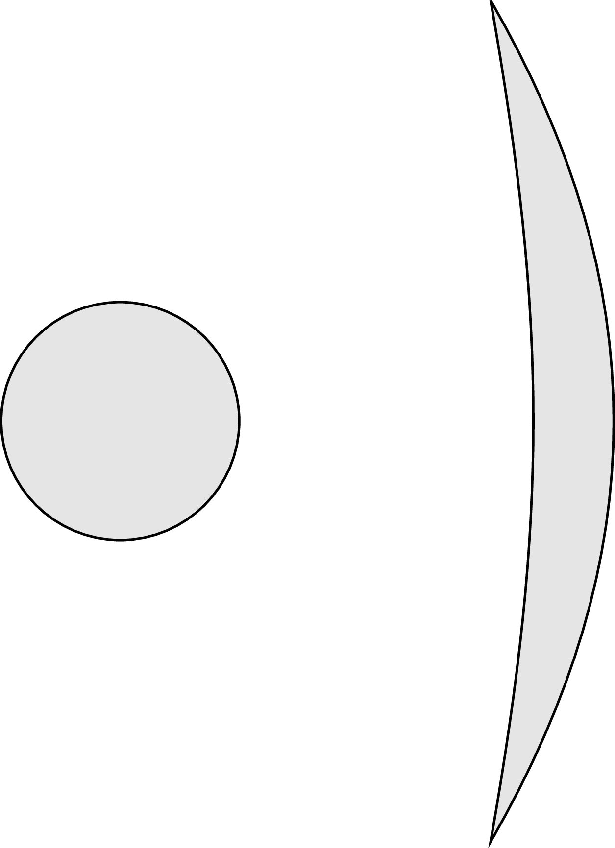
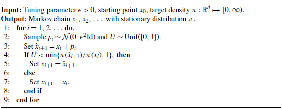
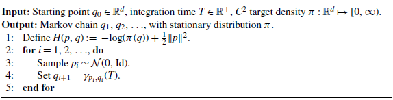
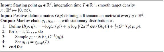
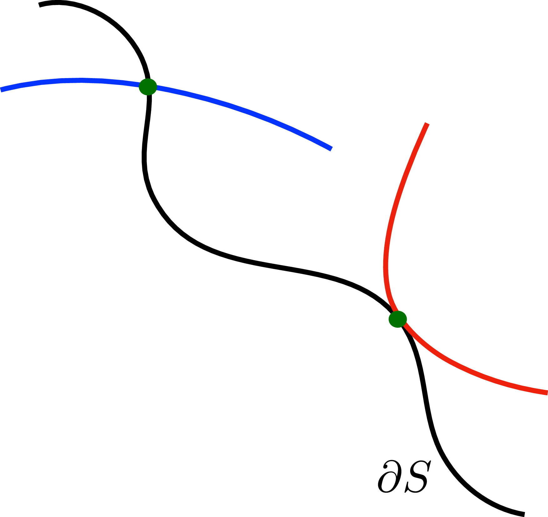


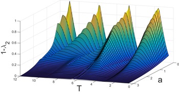

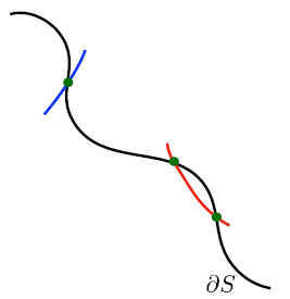

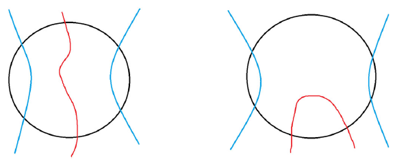


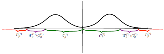


 Open access

