2 Problem statement

We consider a porous medium surrounded by impermeable, no-flow boundaries. This could represent any type of closed reservoir in a field study or sealed rock sample in a laboratory experiment. The medium contains two phases – wetting ($w$), e.g. a liquid and non-wetting ($nw$), e.g. a gas, with different densities $\unicode[STIX]{x1D70C}_{w}$ and $\unicode[STIX]{x1D70C}_{nw}$. The phases are distributed throughout the domain with some initial saturation $S_{w}^{init}(x,y,z)$, where $S_{w}$ is wetting phase saturation, $S_{w}+S_{nw}=1$ and a Cartesian system is used for spatial coordinates. The phases will migrate due to buoyancy and capillary forces until a steady-state is reached, when the fluid and gas are in equilibrium. We seek the saturation distribution $S_{w}(x,y,z)$ at equilibrium, i.e. the final location of the phases.

The equations for the general problem described above are considered to be those describing immiscible flow of two incompressible phases in an incompressible rock and given by mass conservation

(2.1)$$\begin{eqnarray}\unicode[STIX]{x1D719}\frac{\unicode[STIX]{x2202}S_{j}}{\unicode[STIX]{x2202}t}+\unicode[STIX]{x1D735}\boldsymbol{\cdot }\boldsymbol{u}_{j}=0,\end{eqnarray}$$

and Darcy’s law

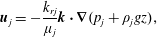(2.2)$$\begin{eqnarray}\boldsymbol{u}_{j}=-\frac{k_{rj}}{\unicode[STIX]{x1D707}_{j}}\boldsymbol{k}\boldsymbol{\cdot }\unicode[STIX]{x1D735}(p_{j}+\unicode[STIX]{x1D70C}_{j}gz),\end{eqnarray}$$

where $\unicode[STIX]{x1D719}$ is the porosity of the rock, $k_{rj}$ the relative permeability to phase $j$ ($j=w$ or $j=nw$), $\unicode[STIX]{x1D707}_{j}$ the viscosity of phase $j$, $p_{j}$ the pressure of phase $j$, $\boldsymbol{u}_{j}$ the Darcy velocity of phase $j$, $\boldsymbol{k}$ the absolute permeability tensor, $g$ is gravitational acceleration and $z$ is the vertical coordinate. Pressures of the non-wetting phase and the wetting phase are related by

(2.3)$$\begin{eqnarray}p_{nw}-p_{w}=P_{c}(S_{w}),\end{eqnarray}$$

where $P_{c}(S_{w})$ is the capillary pressure curve.

When considering gravity driven flow, as opposed to flow driven by injection or production wells, capillary pressure is usually significant and different structures of $P_{c}(S_{w})$ curves will have a drastic effect on the solution. While some gravity segregation models assume the same curves throughout the domain, it is generally more accurate to take into account the spatial change of $P_{c}(S_{w})$. This is typically modelled using the Leverett $J$-function as follows:

(2.4)$$\begin{eqnarray}P_{c}(S_{w},k,\unicode[STIX]{x1D719})=\unicode[STIX]{x1D6FC}C\sqrt{\frac{\unicode[STIX]{x1D719}}{k}}J(S_{w}),\end{eqnarray}$$

where $C$ is a fitting parameter and $\unicode[STIX]{x1D6FC}$ is the $J$-function scaling coefficient, which accounts for interfacial tension, contact angle and unit conversion. Isotropic permeability is assumed here so that $k$ is a scalar function. This is not a requirement for the derivation, but assumed for simplicity to avoid defining $P_{c}$ as a function of the directional components of $k$ (often taken as the average). Two of the most widely used $J$-functions are the van Genuchten (VG) (van Genuchten Reference van Genuchten1980) & Brooks–Corey (BC) (Brooks & Corey Reference Brooks and Corey1966) models given by

(2.5)$$\begin{eqnarray}J_{VG}(S_{w})=[(\widetilde{S}_{w})^{-1/m}-1]^{1-m}\end{eqnarray}$$

and

(2.6)$$\begin{eqnarray}J_{BC}(S_{w})=(\widetilde{S}_{w})^{-1/\unicode[STIX]{x1D706}},\end{eqnarray}$$

respectively, where $\widetilde{S}_{w}=(S_{w}-S_{wi})/(1-S_{wi})$, $S_{wi}$ is the irreducible water saturation and $\unicode[STIX]{x1D706}$, $m$ are fitting parameters. It is evident that hysteresis is not considered in our capillary pressure models (Hilfer Reference Hilfer2006; Pini & Benson Reference Pini and Benson2017). Furthermore, the BC model incorporates capillary entry pressure, i.e. $P_{c}(S_{w}=1)\neq 0$ while in the VG model entry pressure is zero.

We are interested in the solution after the phases have equilibrated and there is no longer any flow. Under these conditions phase velocities are zero everywhere, i.e. $\boldsymbol{u}_{j}=0$, and we immediately obtain from (2.2) that

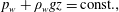(2.7a)$$\begin{eqnarray}\displaystyle & \displaystyle p_{w}+\unicode[STIX]{x1D70C}_{w}gz=\text{const.}, & \displaystyle\end{eqnarray}$$

(2.7b)$$\begin{eqnarray}\displaystyle & \displaystyle p_{nw}+\unicode[STIX]{x1D70C}_{nw}gz=\text{const.}, & \displaystyle\end{eqnarray}$$

(2.8)$$\begin{eqnarray}P_{c}=P_{c}^{0}+\unicode[STIX]{x0394}\unicode[STIX]{x1D70C}gz,\end{eqnarray}$$

where $\unicode[STIX]{x0394}\unicode[STIX]{x1D70C}=\unicode[STIX]{x1D70C}_{w}-\unicode[STIX]{x1D70C}_{nw}$ and $P_{c}^{0}$ (the capillary pressure at $z=0$) is a constant to be determined. Next, we integrate (2.1) over the entire domain and apply the divergence theorem to arrive at the equation

(2.9)$$\begin{eqnarray}\int _{V}\widetilde{S}_{w}(x,y,z)\,\text{d}V=\int _{V}\widetilde{S}_{w}^{init}\,\text{d}V,\end{eqnarray}$$

where the integration here is a volume integral (i.e. triple integral) over the domain volume $V$ and $\widetilde{S}_{w}^{init}=(S_{w}^{init}-S_{wi})/(1-S_{wi})$. Equation (2.9) is simply a statement that total saturation in the domain remains constant over time since we consider a closed reservoir with no flow through the boundaries. It can be expressed in terms of average saturation, i.e. $\langle \widetilde{S}_{w}\rangle =\langle \widetilde{S}_{w}^{init}\rangle$, where $\langle \rangle$ denotes averaging over the entire domain.

The final equation for our problem is the capillary pressure-saturation relationship which can be generally expressed as $P_{c}=f(\unicode[STIX]{x1D719},k,S_{w})$, where $f$ is some known function obtained through laboratory experiments on rock samples. In this work, $f$ is given by (2.4) and (2.5) or (2.6). Equations (2.8), (2.9) and (2.4) are a system of three equations which can be solved to obtain $P_{c}^{0}$, $P_{c}(z)$ and $S_{w}(x,y,z)$. In general, the saturation solution will be obtained by inverting (2.4) and will depend on spatial variation of porosity and permeability as well as the hydrostatic capillary pressure.

We now formulate the governing equations in dimensionless form by defining the following non-dimensional parameters: $N_{b}=\unicode[STIX]{x1D6FC}C/(\unicode[STIX]{x0394}\unicode[STIX]{x1D70C}gh^{2})$, $\widetilde{k}=k/h^{2}$, $\widetilde{P}_{c}^{0}=P_{c}^{0}/(\unicode[STIX]{x0394}\unicode[STIX]{x1D70C}gh)$, $\widetilde{P}_{c}=P_{c}/(\unicode[STIX]{x0394}\unicode[STIX]{x1D70C}gh)$ and $\widetilde{z}=z/h$, where $h$ is the domain height and $N_{b}$ is the Bond number representing a ratio between capillary and gravity forces. Substituting these in the governing equations (2.8) and (2.4) we arrive at

(2.10)$$\begin{eqnarray}\widetilde{P}_{c}=\widetilde{P}_{c}^{0}+\widetilde{z},\end{eqnarray}$$

and

(2.11)$$\begin{eqnarray}\widetilde{P}_{c}=N_{b}\sqrt{\frac{\unicode[STIX]{x1D719}}{\widetilde{k}}}J(S_{w}).\end{eqnarray}$$

The third governing equation is already dimensionless and remains in the form presented in (2.9).

3 Analytical solution

We now derive a solution to the problem formulated in the previous section. It is important to point out that the solution described by (2.9)–(2.11) does not fully account for entry-pressure trapping of phases. When entry pressure is introduced in (2.6), regions with non-zero capillary pressure can be fully saturated with water. This occurs when $\widetilde{P}_{c}<\widetilde{P}_{e}$, where $\widetilde{P}_{e}=N_{b}\sqrt{\unicode[STIX]{x1D719}/\widetilde{k}}$ is the entry pressure. The non-wetting phase will invade these regions only if the surrounding capillary pressure exceeds $\widetilde{P}_{e}$. In these regions, equation (2.10) does not hold and yet the condition $\boldsymbol{u}_{j}=0$ is still fulfilled. We will refer to this type of trapping involving fully saturated regions as entry pressure trapping. In the following, we continue to derive a solution without considering entry pressure trapping, which will be discussed in detail in § 5.

Taking capillary pressure described by (2.11) together with a $J$-function of the form in (2.5) or (2.6), leads to $\widetilde{P}_{c}>0$. However, equation (2.10) is not compatible with this requirement and may result in negative $\widetilde{P}_{c}$ values. We therefore modify (2.10) to avoid negative capillary pressure

(3.1)$$\begin{eqnarray}\widetilde{P}_{c}=\left\{\begin{array}{@{}ll@{}}\widetilde{P}_{c}^{0}+\widetilde{z},\quad & \widetilde{z}>-\widetilde{P}_{c}^{0}\\ 0,\quad & \widetilde{z}\leqslant -\widetilde{P}_{c}^{0}.\end{array}\right.\end{eqnarray}$$

We note that we have considered here $\unicode[STIX]{x0394}\unicode[STIX]{x1D70C}>0$ (heavier wetting phase) by convention, however, this equation can apply to both cases of $\unicode[STIX]{x0394}\unicode[STIX]{x1D70C}>0$ and $\unicode[STIX]{x0394}\unicode[STIX]{x1D70C}<0$ (heavier non-wetting phase). In the first case, $z=0$ is at the top of the domain so that $P_{c}$ decreases with depth, while for the latter case, $z=0$ is at the bottom of the domain and $P_{c}$ increases with depth.

We can now obtain a formula for the saturation distribution by substituting (2.11) with the $J$-function from (2.6) or (2.5) in (3.1) and solving for $\widetilde{S}_{w}$. This results in the solution

(3.2)$$\begin{eqnarray}\widetilde{S}_{w}=\left\{\begin{array}{@{}ll@{}}\displaystyle \left(\left[\frac{1}{N_{b}}\sqrt{\frac{\widetilde{k}(x,y,z)}{\unicode[STIX]{x1D719}(x,y,z)}}(\widetilde{P}_{c}^{0}+\widetilde{z})\right]^{1/(1-m)}+1\right)^{-m},\quad & \widetilde{z}>-\widetilde{P}_{c}^{0}\\ 1,\quad & \widetilde{z}\leqslant -\widetilde{P}_{c}^{0},\end{array}\right.\end{eqnarray}$$

for the VG $J$-function and

(3.3)$$\begin{eqnarray}\widetilde{S}_{w}=\left\{\begin{array}{@{}ll@{}}\displaystyle \left[\frac{1}{N_{b}}\sqrt{\frac{\widetilde{k}(x,y,z)}{\unicode[STIX]{x1D719}(x,y,z)}}(\widetilde{P}_{c}^{0}+\widetilde{z})\right]^{-\unicode[STIX]{x1D706}},\quad & \widetilde{z}>\widetilde{P}_{e}-\widetilde{P}_{c}^{0}\\ 1,\quad & \widetilde{z}\leqslant \widetilde{P}_{e}-\widetilde{P}_{c}^{0},\end{array}\right.\end{eqnarray}$$

for the BC $J$-function. Despite the exclusion of capillary entry trapping in the solution, there is still an impact of $\widetilde{P}_{e}$, which can be seen in (3.3), where saturation is $1$ if $\widetilde{P}_{c}\leqslant \widetilde{P}_{e}$.

The constant $\widetilde{P}_{c}^{0}$ is obtained by substituting (3.2) or (3.3) in (2.9) and solving the integral equation. For some special cases the integral can be solved analytically. This is the case for a homogeneous medium ($k=\text{const.}$ and $\unicode[STIX]{x1D719}=\text{const.}$) with BC type capillary pressure, which leads to the equations

(3.4a)$$\begin{eqnarray}\displaystyle & \displaystyle (\widetilde{P}_{c}^{0})^{1-\unicode[STIX]{x1D706}}-(1+\widetilde{P}_{c}^{0})^{1-\unicode[STIX]{x1D706}}=(\unicode[STIX]{x1D706}-1)\widetilde{P}_{e}^{\unicode[STIX]{x1D706}}\int _{V}\widetilde{S}_{w}^{init}\,\text{d}V, & \displaystyle \text{if }\widetilde{P}_{e}-\widetilde{P}_{c}^{0}\geqslant 1,\end{eqnarray}$$

(3.4b)$$\begin{eqnarray}\displaystyle & \displaystyle \widetilde{P}_{c}^{0}-\frac{\widetilde{P}_{e}^{\unicode[STIX]{x1D706}}(\widetilde{P}_{c}^{0})^{1-\unicode[STIX]{x1D706}}}{1-\unicode[STIX]{x1D706}}=\frac{\unicode[STIX]{x1D706}\widetilde{P}_{e}}{\unicode[STIX]{x1D706}-1}-1+\int _{V}\widetilde{S}_{w}^{init}\,\text{d}V & \displaystyle \text{if }\widetilde{P}_{e}-\widetilde{P}_{c}^{0}<1.\end{eqnarray}$$

$\widetilde{k}(x,y,z)$

$\unicode[STIX]{x1D719}(x,y,z)$

$\widetilde{P}_{c}^{0}$

3.1 Ensemble mean solution

Many applications of flow modelling in porous rocks must incorporate permeability uncertainty, i.e. $k$ values are generally unknown and vary by orders of magnitude over small distances. A common approach for dealing with this problem is to consider $k$ as a random space function (RSF) with known statistical properties and to seek the ensemble mean of the variable of interest. We now extend the previous formulation by considering $k$ to be a stationary and isotropic RSF, log-normally distributed so that the $Y=\ln k$ (log permeability) is characterized by the mean $\langle Y\rangle =\ln k_{G}$ and variance $\unicode[STIX]{x1D70E}_{y}^{2}$. The probability density function of $Y$ is then given by

(3.5)$$\begin{eqnarray}F(Y)=\frac{1}{\sqrt{2\unicode[STIX]{x03C0}\unicode[STIX]{x1D70E}_{y}^{2}}}\exp \left[\frac{-(Y-\ln k_{G})^{2}}{2\unicode[STIX]{x1D70E}_{y}^{2}}\right].\end{eqnarray}$$

The ensemble average over many realizations of permeability $k$ can be calculated by the following expression:

(3.6)$$\begin{eqnarray}\langle \widetilde{S}_{w}\rangle _{E}=\int _{-\infty }^{\infty }\widetilde{S}_{w}(\,\widetilde{y},\widetilde{z})\cdot F(\,\widetilde{y}\,)\,\text{d}\widetilde{y},\end{eqnarray}$$

where $\langle \rangle _{E}$ denotes ensemble average (or expected value) and $\widetilde{y}=\ln \widetilde{k}$.

First, we consider the case of VG capillary pressure. Substituting (3.2) in equation, (3.6) we arrive at

(3.7)$$\begin{eqnarray}\langle \widetilde{S}_{w}\rangle _{E}=\left\{\begin{array}{@{}ll@{}}\displaystyle \int _{-\infty }^{\infty }\left[A(\widetilde{P}_{c}^{0},\widetilde{z})\exp [\frac{\widetilde{y}}{2(1-m)}]+1\right]^{-m}F(\,\widetilde{y}\,)\,\text{d}\widetilde{y},\quad & \widetilde{z}>-\widetilde{P}_{c}^{0}\\ 1,\quad & \widetilde{z}\leqslant -\widetilde{P}_{c}^{0},\end{array}\right.\end{eqnarray}$$

where $A=[(\widetilde{P}_{c}^{0}+\widetilde{z})/(N_{b}\sqrt{\unicode[STIX]{x1D719}})]^{1/(1-m)}$ includes all the deterministic parameters. Porosity is considered here to be constant as it typically varies much less than $k$. The integral in (3.7) can be solved numerically, however, we continue the derivation to arrive at a fully analytical expression. The details are presented in appendix A and the final result is given by

(3.8)$$\begin{eqnarray}\langle \widetilde{S}_{w}\rangle _{E}=\left\{\begin{array}{@{}ll@{}}\displaystyle \mathop{\sum }_{n=0}^{\infty }\binom{-m}{n}\{A^{n}B(n)\operatorname{erfc}[C(n)],\quad & \widetilde{z}>-\widetilde{P}_{c}^{0}\\ \qquad +\,A^{-n-m}B(-n-m)\operatorname{erfc}[-C(-n-m)]\},\quad & \\ 1,\quad & \widetilde{z}\leqslant -\widetilde{P}_{c}^{0},\end{array}\right.\end{eqnarray}$$

where

$$\begin{eqnarray}\displaystyle & \displaystyle B(\unicode[STIX]{x1D712})={\textstyle \frac{1}{2}}\exp \{\unicode[STIX]{x1D712}[\unicode[STIX]{x1D712}\unicode[STIX]{x1D70E}_{y}^{2}-4(m-1)\ln \widetilde{k}_{G}]/[8(m-1)^{2}]\}, & \displaystyle \nonumber\\ \displaystyle & \displaystyle C(\unicode[STIX]{x1D712})=-\frac{\unicode[STIX]{x1D712}\unicode[STIX]{x1D70E}_{y}^{2}+2(m-1)[2(m-1)\ln A-\ln \widetilde{k}_{G}]}{\sqrt{8\unicode[STIX]{x1D70E}_{y}^{2}}\cdot (m-1)}, & \displaystyle \nonumber\end{eqnarray}$$

and $\binom{-m}{n}=-m\cdot (-m-1)\cdot \ldots (-m-n+1)/n!$ are the binomial coefficients for any real valued $m$ and natural number $n$. The solution for mean saturation is thus given by (3.8) together with (2.9) which is used for obtaining $\widetilde{P}_{c}^{0}$ in $A$.

Next, we consider BC capillary pressure and substitute equation (3.3) into (3.6). The piecewise function in this case depends on the variable of integration $\widetilde{y}$ since $\widetilde{P}_{e}$ is a function of permeability. Therefore we separate the integration limits into two ranges as follows:

(3.9)$$\begin{eqnarray}\langle \widetilde{S}_{w}\rangle _{E}=\left(\frac{\widetilde{P}_{c}^{0}+\widetilde{z}}{N_{b}\sqrt{\unicode[STIX]{x1D719}}}\right)^{-\unicode[STIX]{x1D706}}\int _{-\infty }^{\widetilde{y}^{\ast }}\exp [-\unicode[STIX]{x1D706}\widetilde{y}/2]F(\,\widetilde{y}\,)\,\text{d}\widetilde{y}+\int _{\widetilde{y}^{\ast }}^{\infty }F(\,\widetilde{y}\,)\,\text{d}\widetilde{y},\end{eqnarray}$$

where $\widetilde{y}^{\ast }=-\unicode[STIX]{x1D706}\ln D$ is the value of $\widetilde{y}$ in which $\widetilde{P}_{e}=\widetilde{P}_{c}^{0}$ and $D=(\widetilde{P}_{c}^{0}+\widetilde{z})/(N_{b}\sqrt{\unicode[STIX]{x1D719}})$. Solving the integrals in (3.9) and rearranging we arrive at the solution

(3.10)$$\begin{eqnarray}\displaystyle \langle \widetilde{S}_{w}\rangle _{E} & = & \displaystyle \frac{1}{2}D^{-\unicode[STIX]{x1D706}}\exp \left[\unicode[STIX]{x1D706}\left(\frac{\unicode[STIX]{x1D706}}{8}\unicode[STIX]{x1D70E}_{y}^{2}-4\ln \widetilde{k}_{G}\right)\right]\operatorname{erfc}\left[\frac{-2\ln \widetilde{k}_{G}-\unicode[STIX]{x1D706}\ln D+\unicode[STIX]{x1D706}\unicode[STIX]{x1D70E}_{y}^{2}}{\sqrt{8\unicode[STIX]{x1D70E}_{y}^{2}}}\right]\nonumber\\ \displaystyle & & \displaystyle +\,\frac{1}{2}\operatorname{erfc}\left[\frac{\unicode[STIX]{x1D706}\ln D+\ln \widetilde{k}_{G}}{\sqrt{2\unicode[STIX]{x1D70E}_{y}^{2}}}\right].\end{eqnarray}$$

The above solution does not incorporate entry-pressure trapping, as mentioned previously regarding the formulation of (3.3).

4 Results – no entry pressure

This section will present an analysis of the solution derived previously considering cases without capillary entry pressure. Capillary pressure is modelled with the VG relationship given by (2.4) with heterogeneous permeability $k(x,y,z)$ and (2.5) as the $J-$function. Throughout this work, analytical solutions will be compared to numerical results obtained using Stanford’s General Purpose Research Simulator, (known as GPRS) (Cao Reference Cao2002) on simulation grids of $25\times 25\times 50$. A finer grid of $50\times 50\times 100$ was also used to test for convergence, which was in fact achieved. Furthermore, in the following, the non-wetting phase will be addressed as CO$_{2}$ and the wetting phase as water, keeping in mind CO$_{2}$ storage applications.

A permeability realization is generated using the sequential Gaussian simulation (Deutsch & Journel Reference Deutsch and Journel1992) module of the Stanford Geostatistical Modeling Software, (known as SGeMS) (Remy, Boucher & Wu Reference Remy, Boucher and Wu2009). The realization is taken to have geometric mean $k_{G}=100$ md, variance of log permeability $\unicode[STIX]{x1D70E}_{y}^{2}=1$ ($Y=\ln k$) and dimensionless correlation length $l_{x}=l_{y}=l_{z}=0.1$ in the $x,y$ and $z$ directions (non-dimensionalized by the domain length in the corresponding direction). The dimensionless permeability is then substituted in (3.2) and together with the solution to (2.9) for $\widetilde{P}_{c}^{0}$, we obtain the saturation distribution. Porosity is taken to be constant ($\unicode[STIX]{x1D719}=0.25$) for simplicity, since it usually has much smaller variations than permeability. Values of $\unicode[STIX]{x0394}\unicode[STIX]{x1D70C}g=9.16~\text{kPa}~\text{m}^{-1}$, $m=0.75$ and $h=0.098~\text{m}$ are assumed and used also for simulation input.

Figure 1.

The CO$_{2}$ saturation distribution in a vertical slice through the domain centre. Plots (a,c,e) are results for analytical solution while (b,d,f) are numerical simulations. The first row of plots (a,b) are results for $N_{b}=7.8$, the second row (c,d) is for $N_{b}=78$ and the last row (e,f) is for $N_{b}=780$.

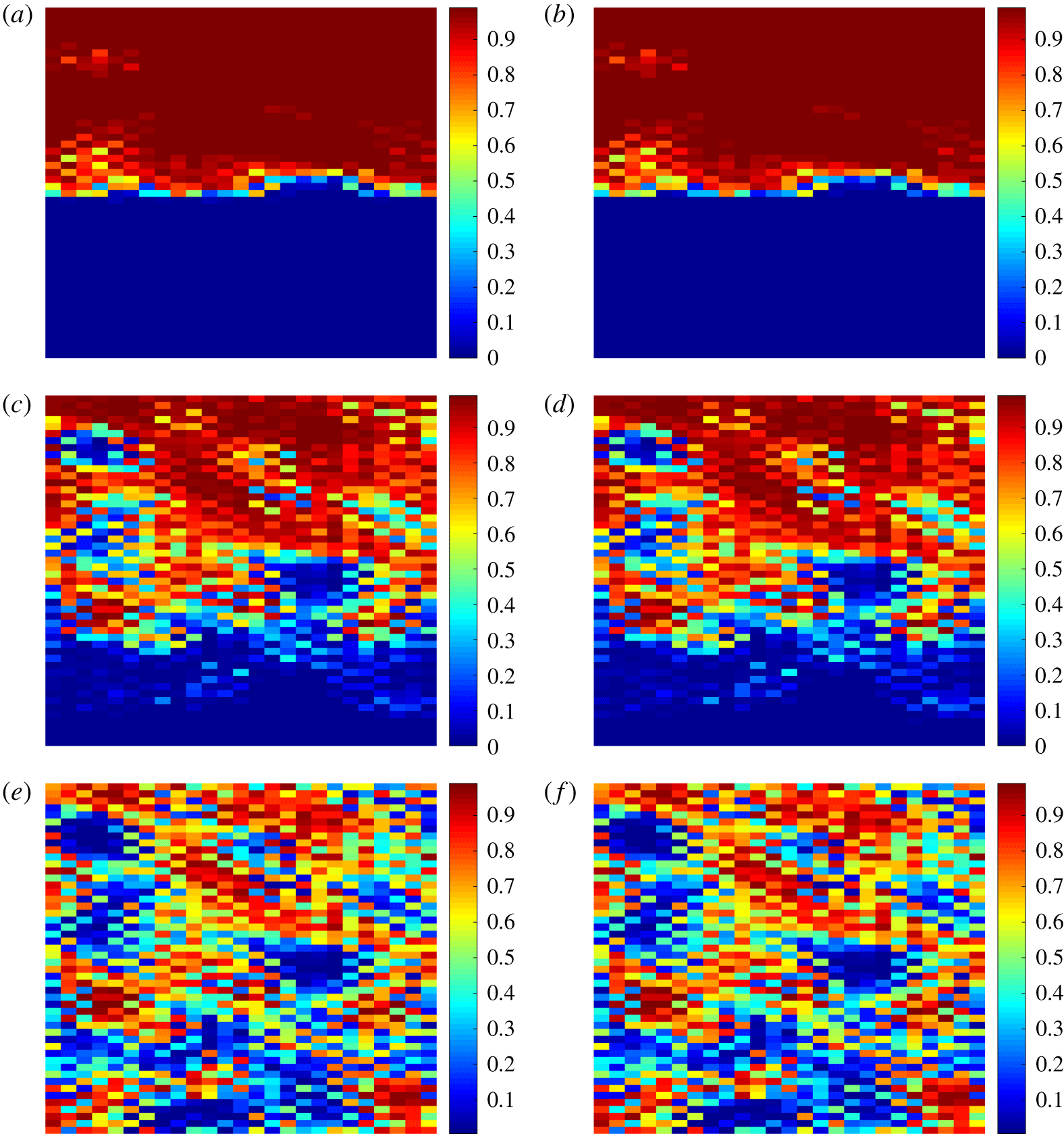
Figure 1 presents results for CO$_{2}$ saturation distribution in a slice through the centre of the cubical domain for three different Bond numbers: a small value of $N_{b}=7.8$, a medium value of $N_{b}=78$ and a large value of $N_{b}=780$. Parameter values in this work often seem arbitrary because they are generally calculated from dimensional values which are used as input in the simulator. The left-hand column of plots (a,c,e) are analytical results while the right-hand column (b,d,f) are simulation results. A uniform initial mixture of water and CO$_{2}$ is assumed in the domain, i.e. $\widetilde{S}_{w}^{init}=0.5$ is used in the simulations leading to $\langle \widetilde{S}_{w}^{init}\rangle =0.5$. It is clear that there is an excellent agreement between analytical and numerical solutions for all cases.

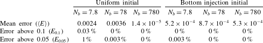
Saturation errors ($E$) are presented in table 1 (‘uniform initial’), calculated by $E=|S_{w}^{numerical}-S_{w}^{analytical}|$ at every grid block. Mean error is calculated as $\langle E\rangle$, averaging over all grid block errors. The portion of the domain with an error above a threshold value is calculated by $E_{a}=N(E>a)/N$, i.e. the number of grid blocks with error above threshold $a$ divided by the total number of grid blocks ($N$). The results presented in table 1 show small errors in all cases and for all measure types. The above analysis is an example of utilizing the analytical solution for validation of a numerical code. In this specific case the match is excellent, showing that the simulation resolution is sufficiently high.

The case of small capillary pressure values corresponding to $N_{b}=7.8$ (figure 1a,b) shows a gravity dominated regime with almost complete segregation. Still, capillary pressure is not completely negligible and some spatial variation of $\widetilde{S}_{\text{CO}_{2}}$ is seen as a result of trapping. The case of large capillary pressure corresponding to $N_{b}=780$ (figure 1e,f) shows a capillary dominated regime in which $\widetilde{S}_{\text{CO}_{2}}$ is distributed throughout the domain with many regions of trapped phases. Increasing values of $N_{b}$ above $780$ or decreasing below $7.8$ will not have a significant impact on the solutions in figures 1(a,b) and 1(e,f), respectively. The case of $N_{b}=78$ in figure 1(c,d) shows a gravity–capillary regime in which both partial segregation and capillary effects are present.

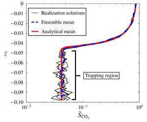
Figure 2 presents plane averaged $\widetilde{S}_{w}$ as a function of $\widetilde{z}$. The transition from gravity dominated to capillary dominated conditions can be observed in the profiles. For $N_{b}=7.8$, $\widetilde{P}_{c}$ values are small and gravity dominates, which results in significant segregation between phases (red curve) and many values of $\widetilde{S}_{w}=0$ or $1$ in (3.2) (seen when taking $N_{b}\rightarrow 0$). For $N_{b}=780$, the $\widetilde{P}_{c}$ curve is large and therefore capillarity dominates, leading to capillary limit saturation distribution (light blue line), i.e. variation of $\widetilde{S}_{w}$ with $\widetilde{z}$ around the value of $\langle \widetilde{S}_{w}^{init}\rangle$. The variations are a results of heterogeneity $\widetilde{k}(x,y,z)$ and for a homogeneous medium the result would be simply $\widetilde{S}_{w}=\langle \widetilde{S}_{w}^{init}\rangle$. In between the two limits of gravity and capillary dominance, e.g. $N_{b}=78$ in figure 2, both gravity and capillary effects are apparent.

Figure 2.

Horizontally averaged saturation as a function of height for different values of parameter $N_{b}$ considering VG capillary pressure. Analytical results (solid lines) given by (3.2) and (2.9) are compared with numerical simulation results (dashed lines).

Table 1.

Error $E=|S_{w}^{numerical}(x,y,z)-S_{w}^{analytical}(x,y,z)|$ for different values of $N_{b}$ and considering two cases of initial conditions: uniform $\widetilde{S}_{w}^{init}=0.5$ and bottom injection of $\langle \widetilde{S}_{\text{CO}_{2}}^{init}\rangle =0.1$ (figure 3a).

Figure 3.

The CO$_{2}$ saturation distribution in a vertical slice through the domain centre for (a) initial time ($\widetilde{S}_{\text{CO}_{2}}^{init}(x,y,z)$), (b) equilibrium analytical solution and (c) equilibrium numerical solution.

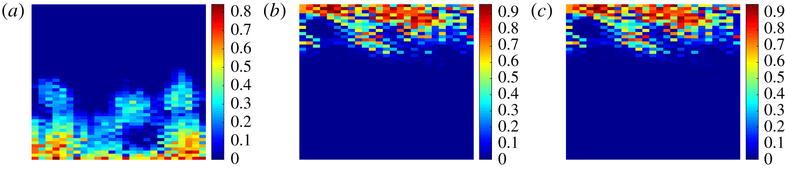
Figure 3(a–c) presents results for a different initial saturation distribution, i.e. not a constant $\widetilde{S}_{w}^{init}=0.5$ as previously considered. In general, the solution does not depend on the initial distribution and only requires knowledge of the total initial saturation (right-hand side of (2.9)). However, the numerical solution is obtained by simulating the full time evolution from initial condition to steady-state and therefore may be affected by $\widetilde{S}_{\text{CO}_{2}}^{init}$ (due to numerical error). To test this, we assume an arbitrary saturation distribution shown in figure 3(a), obtained by injecting CO$_{2}$ at the bottom of the domain. The steady-state equilibrium results are shown in figures 3(b) and 3(c) for analytical and numerical results, respectively. Excellent agreement can be seen. Further validation was conducted by a grid-by-grid error calculation and presented in table 1 (‘bottom injection initial’) where minuscule errors are shown. It is therefore concluded that for the VG case, the numerical solution does not depend on the initial distribution, as expected. There is, however, a dependence on the overall average initial saturation $\langle \widetilde{S}_{\text{CO}_{2}}^{init}\rangle$. The results in figure 3(b,c) are for the same parameter as in figure 1(c,d) and thus we can observe the impact of a smaller $\langle \widetilde{S}_{\text{CO}_{2}}^{init}\rangle$. For the former case, $\langle \widetilde{S}_{\text{CO}_{2}}^{init}\rangle =0.5$ while for the latter case $\langle \widetilde{S}_{\text{CO}_{2}}^{init}\rangle =0.1$ and in fact the smaller CO$_{2}$ region is apparent in figures 3(b) and 3(c).

4.1 Ensemble mean results

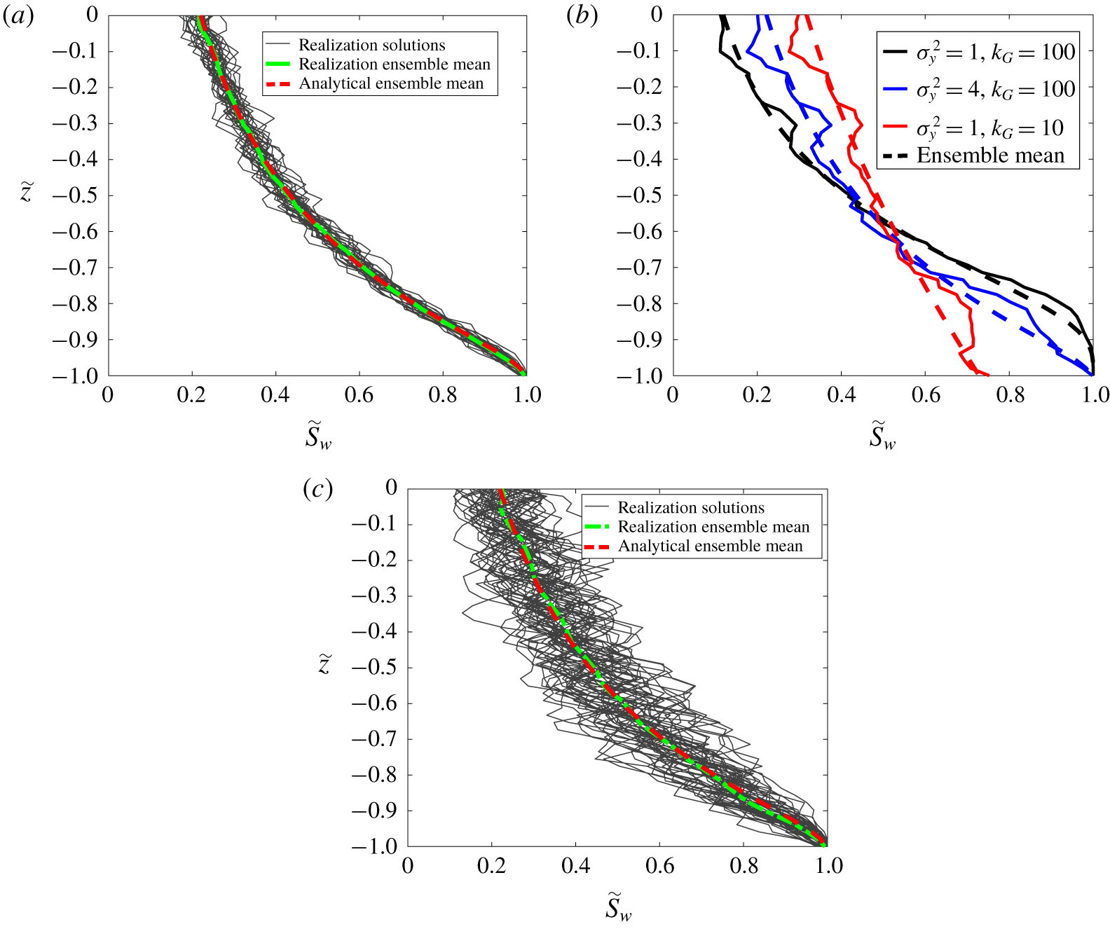
The ensemble average solution presented in § 3.1 will be discussed now. Figures 4 and 5 present ensemble mean saturation profiles given by (3.8) and (2.9). In figure 4(a) we present the case of $N_{b}=7.8$, $\unicode[STIX]{x1D719}=0.25$, $m=0.75$, $\langle \widetilde{S}_{\text{CO}_{2}}^{init}\rangle =0.5$, $\unicode[STIX]{x1D70E}_{y}^{2}=4$ and $\ln \widetilde{k}_{G}=-25.3$ (corresponding to $k_{G}=100~\text{md}$) using a dashed red line. We also plot horizontally averaged $S_{w}$ for the same problem parameters using 30 different $k$ realizations via calculations from (3.2) and (2.9) (thin grey lines). It is clear that the saturation profiles of the 30 realizations surround the ensemble mean solution closely and the scatter is quite small. This indicates that our derivation for $\langle \widetilde{S}_{w}\rangle _{E}$ is correct and that the $k$ sample size is sufficiently large so horizontal averaging (used to obtain the profiles) leads to fairly similar curves. Furthermore, we plot the ensemble average of the 30 realizations using a solid green line and show that the result coincides with the analytical ensemble mean. In fact only a few realizations are needed to converge to the green line.

Figure 4.

Comparison between ensemble mean solution (equation (3.8)) and solutions using permeability realizations (equation (3.2)) for (a) 30 realizations of the case $\unicode[STIX]{x1D70E}_{y}^{2}=4$, $\ln \widetilde{k}_{G}=-25.3$, (b) one realization of three cases specified in legend and (c) 30 realizations for $\unicode[STIX]{x1D70E}_{y}^{2}=4$, $\ln \widetilde{k}_{G}=-25.3$ with $l_{x}=l_{y}=0.25$ and $l_{z}=0.1$.

Figure 5.

Ensemble mean saturation profiles for varying $\unicode[STIX]{x1D70E}_{y}^{2}$.

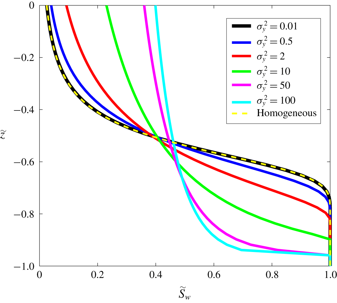
Figure 4(b) shows that even the solution for a single realization (solid lines) follows the ensemble mean profiles (dashed lines) closely for three different cases with varying parameters. For sufficiently large $k$ samples, corresponding to a fine grid mesh, the horizontal averaging is responsible for the fairly close match. It is an expression of ergodic theory, stating that under conditions of $k$ stationarity and small correlation lengths compared with domain lengths ($l_{x},l_{y},l_{z}\ll 1$), ensemble averaging can be substituted with spatial averaging. Figure 4(c) presents results for statistically anisotropic permeability. It is seen that heterogeneity structures which are horizontally elongated ($l_{x},l_{y}>l_{z}$) lead to significantly more erratic saturation curves as permeability differences between layers are increased and the condition $l_{x},l_{y}\ll 1$ is fulfilled to a lesser extent. Nevertheless, the average saturation given by (3.8) and (2.9) does not depend on anisotropy and despite the large saturation variations between different layers, the ensemble average of the realizations (green dashed curve) matches the analytical result (red dashed curve).

The analytical solution given by (3.8) allows us to analyse the impact of heterogeneity on the saturation either by scanning different parameter values or by considering the limits of large/small parameters directly in the equations. Figure 5 illustrates the impact of log permeability variance on the solution. For low variance (e.g. $\unicode[STIX]{x1D70E}_{y}^{2}=0.01$) the solution tends to that of a homogeneous medium with permeability $k=k_{G}$, seen by comparing the black solid and yellow dashed curves. As $\unicode[STIX]{x1D70E}_{y}^{2}$ increases, there are more capillary effects leading to less variability of saturation and a smaller fully water saturated zone at the bottom of the domain. However, at the limit of high variance (e.g. $\unicode[STIX]{x1D70E}_{y}^{2}=100$) the solution is not capillary dominated, as was discussed in figure 2 ($N_{b}=780$) with saturation values around $\langle \widetilde{S}_{w}^{init}\rangle$, but rather presents a varying saturation profile (light blue curve).

5 Results with entry pressure

We now turn to study gravity segregation with BC capillary pressure, i.e. $P_{c}$ is given by (2.4) and (2.6). The main difference from the VG case is the capillary entry pressure, which is non-zero and changes spatially with permeability. Observing equation (3.3), we see that $\widetilde{S}_{w}=1$ is now obtained when $\widetilde{z}<\widetilde{P}_{e}-\widetilde{P}_{c}^{0}$, which is spatially varying with $\widetilde{k}$. This means that regions which are completely water saturated can exist at the same level $\widetilde{z}$ as regions with CO$_{2}$. This does not occur in the VG case. The second and perhaps more significant impact of $\widetilde{P}_{e}$ is capillary entry trapping, which is not captured at all by the equilibrium analytical solution. During the dynamic migration of the fluids, regions with CO$_{2}$ will not invade a fully water saturated region unless their capillary pressure exceeds the entry pressure of the fully saturated zone. This leads to an equilibrium solution in which some regions with large entry pressure remain with $\widetilde{S}_{w}=1$ since they are surrounded by zones of low capillary pressure (trapped water) or regions of small capillary pressure surrounded by $\widetilde{S}_{w}=1$ zones with large entry pressure (trapped CO$_{2}$). Our numerical solution, however, includes the time evolution and incorporates capillary entry trapping (see Li (Reference Li2011) for details).

Figure 6.

The CO$_{2}$ saturation distribution in a vertical slice through the domain centre for BC capillary pressure. Plots (a,c,e) are results for analytical solution while (b,d,f) are numerical simulations. The first row of plots (a,b) are results for $N_{b}=7.8$, the second row (c,d) is for $N_{b}=78$ and the last row (e,f) is for $N_{b}=780$.

Figure 7.

Dimensionless capillary pressure $\widetilde{P}_{c}$ in a vertical slice through the domain centre corresponding to figure 6(b). Inset: enlargement of a region with trapped CO$_{2}$ as a result of entry pressure trapping (indicated in figure 6b by a red rectangle).

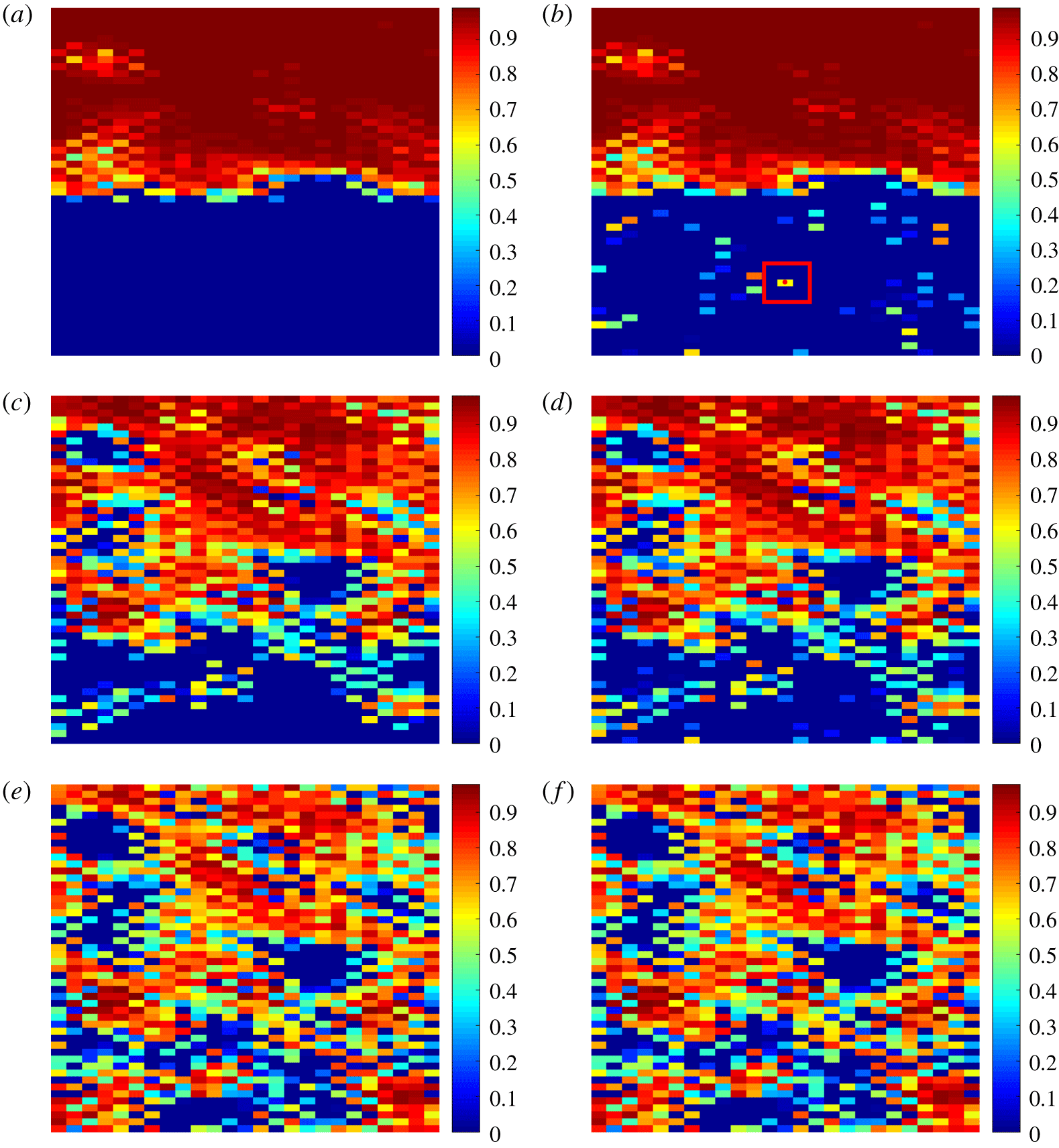
Figure 6 presents results for CO$_{2}$ saturation distribution in a slice through the domain centre for both analytical (panels a,c,e) and numerical (panels b,d,f) calculations. Parameters of $\unicode[STIX]{x1D706}=2$ and uniform $\widetilde{S}_{\text{CO}_{2}}^{init}=0.5$ are taken. Three values of $N_{b}$ are considered spanning from gravity to capillary dominated regimes, as was presented in figure 1 for the VG case. In fact, there is a similarity between the two figures since the parameters and the permeability field are the same, however, differences are apparent (particularly for panels c and d) due to the different $\widetilde{P}_{c}$ functions. A comparison between analytical and numerical results in figure 6 shows much agreement, but also substantial differences. For example, in figures 6(b) and 6(d), there is trapped CO$_{2}$ in the lower regions, which are completely water saturated according to the analytical solution. Errors are presented quantitatively in table 2, where for the capillary dominated case ($N_{b}=780$, figure 6(e,f)) they are very small. Error increases with lower values of $N_{b}$ as the fully water saturated region becomes larger. This region is where the numerical solution presents entry pressure trapping of CO$_{2}$ which cannot be predicted by the analytical solution.

Table 2.

Error $E=|S_{w}^{numerical}(x,y,z)-S_{w}^{analytical}(x,y,z)|$ for different values of $N_{b}$ and considering two cases of initial conditions: uniform $\widetilde{S}_{\text{CO}_{2}}^{init}=0.5$ and bottom injection of $\langle \widetilde{S}_{\text{CO}_{2}}^{init}\rangle =0.1$ (figure 3a).

To understand the entry pressure trapping presented in the numerical solution we plot the capillary pressure $\widetilde{P}_{c}$ corresponding to figure 6(b). This is presented in figure 7. It is apparent that the top region, down to approximately $\widetilde{z}=-0.5$, has hydrostatic $\widetilde{P}_{c}$ variation in accordance to (3.1). In this region the analytical solution is in fairly good agreement with the numerical. However, below this region $\widetilde{P}_{c}$ changes erratically from grid block to grid block. The majority of grid blocks in this lower region are fully water saturated and therefore capillary pressure is not well defined. The numerical simulator assigns the entry pressure to these grid blocks as virtual capillary pressure. Thus the observed erratic variation in the lower part of figure 7 is in fact the impact of permeability variation on entry pressure.

A grid block with trapped CO$_{2}$ will have lower capillary pressure than all of its neighbouring grid blocks which results in a CO$_{2}$ pressure gradient pointing towards this block ($p_{\text{CO}_{2}}=p_{w}+P_{c}$). Since the surrounding blocks are all fully water saturated, no CO$_{2}$ can in fact migrate and the CO$_{2}$ is trapped. An example for such a grid block is presented in the inset of figure 7, where the centre block consists of $\widetilde{S}_{w}=0.38$ and is surrounded by $\widetilde{S}_{w}=1$ neighbouring blocks. This enlarged region can also be observed in figure 6(b), marked with a red rectangle, showing the trapped CO$_{2}$. Whether a grid block will contain trapped CO$_{2}$ or not depends on the time evolution of capillary pressure and saturation, which makes it very difficult to estimate analytically using a steady-state approach. In the next section we will discuss a method for estimating this trapping.

Figure 8 presents results for the horizontally averaged water saturation profiles. The same conclusion that was discussed for figure 6 can be drawn here, i.e. a match between analytical and numerical results is seen for the case of $N_{b}=780$ while error is seen at the lower parts in cases $N_{b}=7.8,78$ for the analytical solution. Overall, the errors in the case of uniform $\widetilde{S}_{\text{CO}_{2}}^{init}=0.5$ can be considered reasonable (see left-hand side of table 2) and the analytical solution is useful. This is not so for the next case, when we consider smaller amounts of initial CO$_{2}$ saturation.

Figure 8.

Horizontally averaged saturation as a function of height for different values of parameter $N_{b}$ considering BC capillary pressure and uniform $\widetilde{S}_{\text{CO}_{2}}^{init}=0.5$. Analytical results (solid lines) given by (3.3) and (2.9) are compared with numerical simulation results (dashed lines).

Figure 9.

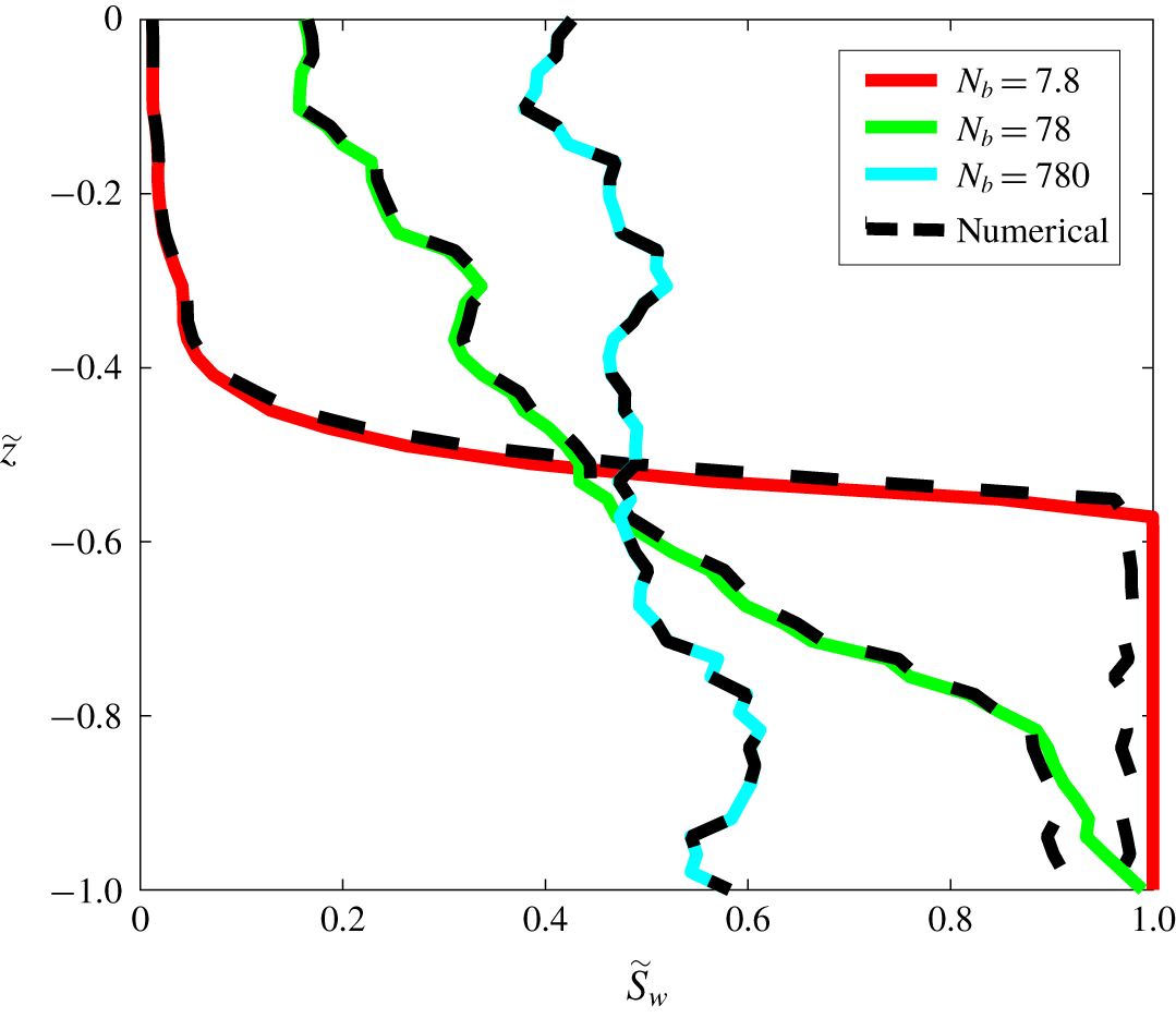
The CO$_{2}$ saturation distribution in a vertical slice through the centre of the rectangular domain for BC capillary pressure and initial bottom injection of $\langle \widetilde{S}_{\text{CO}_{2}}^{init}\rangle =0.1$. Plots (a,c,e) are results for analytical solution while (b,d,f) are numerical simulations. The first row of plots (a,b) are results for $N_{b}=7.8$, the second row (c,d) is for $N_{b}=78$ and the last row (e,f) is for $N_{b}=780$.

Figure 9 presents results for CO$_{2}$ saturation distribution for the case of $\widetilde{S}_{\text{CO}_{2}}^{init}$ as presented in figure 3(a), i.e. following injection of $\langle \widetilde{S}_{\text{CO}_{2}}^{init}\rangle =0.1$ at the domain bottom. When entry pressure is included the equilibrium solution is no longer independent of the initial distribution $\widetilde{S}_{\text{CO}_{2}}^{init}(x,y,z)$. Results of numerical simulations are strikingly different than the analytical solution here, particularly for the $N_{b}=78$ case (figure 9c,d). For all three values of $N_{b}$ the numerical results show significantly more CO$_{2}$ at the lower parts of the domain. The right-hand side of table 2 presents errors for this case, showing the extent of the mismatch. The largest error is for the case with significant effect of both gravity and capillarity ($N_{b}=78$), where 31 % of the grid blocks have more than 0.05 error and 27 % have error larger than 0.1.

The capillary dominated case presented in figure 9(e,f) is of particular significance. One of the most popular methods for dealing with the computationally demanding CO$_{2}$ migration models is to apply capillary limit upscaling (Mouche et al. Reference Mouche, Hayek and Mügler2010; Behzadi & Alvarado Reference Behzadi and Alvarado2012; Rabinovich et al. Reference Rabinovich, Itthisawatpan and Durlofsky2015; Rabinovich, Li & Durlofsky Reference Rabinovich, Li and Durlofsky2016; Rabinovich Reference Rabinovich2018). This method entails assuming capillary equilibrium, uniform capillary pressure and subsequently the spatial distribution of $\widetilde{S}_{w}$ is obtained. Figure 9(e) is the saturation distribution under this assumption ($\widetilde{P}_{c}$ is approximately constant in the domain). However, this assumption does not incorporate entry pressure trapping during migration, which leads to regions with non-uniform capillary pressure and additional trapped CO$_{2}$ in lower regions, as observed in figure 9(f). This example leads us to the conclusion that under certain conditions, saturation derived from capillary limit assumptions may significantly deviate from the actual saturation distribution (see errors in table 2) and upscaling errors may follow.

5.1 Estimation of capillary entry pressure trapping

We have previously established that the analytical solution in this work does not include the capillary entry pressure trapping and therefore may incur significant error. We now proceed by presenting a heuristic method for extending the solution of (3.3) and (2.9) to apply to cases with trapping. First, the main assumptions considered here will be detailed. In the previous results of § 5 we show that the analytical solution for the case with $\langle \widetilde{S}_{\text{CO}_{2}}^{init}\rangle =0.5$ is reasonably accurate while for $\langle \widetilde{S}_{\text{CO}_{2}}^{init}\rangle =0.1$ there is significant error. We therefore aim to improve cases with small values of $\langle \widetilde{S}_{\text{CO}_{2}}^{init}\rangle$, generally between 0 and 0.15. This is also in line with applications of CO$_{2}$ storage, where it is expected that the volumes of injected CO$_{2}$ will be much smaller than the aquifer volume. Furthermore, we will limit our discussion to low-medium capillary numbers, i.e. approximately $N_{b}<33$. This should apply to many cases, particularly reservoir scale problems, in which $h$ is tens of metres ($N_{b}\propto 1/h^{2}$). Finally, we aim at estimating only the average saturation in each layer of the domain, i.e. obtaining $\langle \widetilde{S}_{w}\rangle _{h}(\,\widetilde{z}\,)$, where $\langle \rangle _{h}$ denotes averaging horizontally. The full solution $\widetilde{S}_{w}(x,y,z)$ with entry trapping will not be estimated here.

A couple of tests are conducted on the solutions with entry pressure trapping to determine sensitivity to some parameters. First, we verify that the solution scales with $\unicode[STIX]{x0394}\unicode[STIX]{x1D70C}gh^{2}$ so we can continue to work with the dimensionless $N_{b}$ parameter. This is carried out by conducting simulations with different $\unicode[STIX]{x0394}\unicode[STIX]{x1D70C}$ but maintaining the same $N_{b}$ and observing no change in the solution. Then, the impact of different injection locations is tested and results are presented in figure 10(a–d) for the following configurations, respectively: uniform $\widetilde{S}_{\text{CO}_{2}}^{init}$, uniform injection at the bottom domain boundary, injection at the centre point of the bottom boundary and injection at a bottom corner point of the domain.

Each of the four cases leads to a significantly different $\widetilde{S}_{\text{CO}_{2}}^{init}$ distribution, however, all have the same average of $\langle \widetilde{S}_{\text{CO}_{2}}^{init}\rangle =0.053$ and same problem parameters. It can be seen that the equilibrium solution does change with different initial conditions as opposed to the VG case which only depends on $\langle \widetilde{S}_{\text{CO}_{2}}^{init}\rangle$. However, the change is relatively small and saturation distribution is quite similar in all four cases. We quantify the amount of trapped CO$_{2}$ in each case, indicated at the bottom of each plot. It can be seen that a significant amount of CO$_{2}$ (almost half) remains trapped via the entry pressure trapping mechanism, while the rest is in the confined space at the top four layers of the model. The relatively small impact of $\widetilde{S}_{\text{CO}_{2}}^{init}$ distribution is seen considering the small difference in the trapped $\langle \widetilde{S}_{w}\rangle$ between the four cases. From here on we will develop the solution for uniform $\widetilde{S}_{\text{CO}_{2}}^{init}$ with the understanding that it should apply to many other $\widetilde{S}_{\text{CO}_{2}}^{init}$ distributions. Nevertheless, we only tested different types of bottom injection and other configurations such as top injection may present much less trapping as the CO$_{2}$ will not reach the bottom layers.

Figure 10.

The CO$_{2}$ saturation distribution in a vertical slice through the centre of the domain for different initial conditions: (a) uniform, (b) bottom uniform injection, (c) bottom centre point injection and (d) bottom corner point injection. All cases consist of $\langle \widetilde{S}_{\text{CO}_{2}}^{init}\rangle =0.053$.

The new solution, which includes entry pressure trapping, is given by

(5.1)$$\begin{eqnarray}\widetilde{S}_{w}=\left\{\begin{array}{@{}ll@{}}\displaystyle \left[\frac{1}{N_{b}}\sqrt{\frac{\widetilde{k}(x,y,z)}{\unicode[STIX]{x1D719}(x,y,z)}}\widetilde{P}_{c}^{new}(\,\widetilde{z}\,)\right]^{-\unicode[STIX]{x1D706}},\quad & \widetilde{P}_{e}<\widetilde{P}_{c}^{new}\\ 1,\quad & \widetilde{P}_{e}\geqslant \widetilde{P}_{c}^{new},\end{array}\right.\end{eqnarray}$$

where

(5.2)$$\begin{eqnarray}\widetilde{P}_{c}^{new}(\,\widetilde{z}\,)=\left\{\begin{array}{@{}ll@{}}\widetilde{P}_{c}^{0}+\widetilde{z},\quad & \widetilde{z}\geqslant \widetilde{z}^{trap}\\ \widetilde{P}_{c}^{trap}(\,\widetilde{z}\,),\quad & \widetilde{z}<\widetilde{z}^{trap}\;\& ;\;\boldsymbol{x}\in \boldsymbol{x}_{trap}\\ 0,\quad & \widetilde{z}<\widetilde{z}^{trap}\;\& \;\boldsymbol{x}\notin \boldsymbol{x}_{trap}.\end{array}\right.\end{eqnarray}$$

It represents the saturation distribution resulting from a new composite capillary pressure profile $\widetilde{P}_{c}^{new}$, which combines the original capillary pressure $\widetilde{P}_{c}^{0}+\widetilde{z}$ and the capillary pressure in the trapping region $\widetilde{P}_{c}^{trap}(\,\widetilde{z}\,)$, to be defined in the following. Only certain regions, i.e. $\boldsymbol{x}_{trap}$ (to be defined in the following) which are prone to trapping are given $\widetilde{P}_{c}^{trap}(\,\widetilde{z}\,)$ and all other regions have hydrostatic or zero $\widetilde{P}_{c}$. The transition between the two capillary pressure functions occurs at $\widetilde{z}^{trap}$, which is simply the intersection of functions, i.e. $\widetilde{P}_{c}^{trap}(\,\widetilde{z}^{trap})=\widetilde{P}_{c}^{0}+\widetilde{z}^{trap}$.

Figure 11.

(a) Dimensionless capillary entry pressure $\widetilde{P}_{e}=\unicode[STIX]{x1D6FC}C\sqrt{k/\unicode[STIX]{x1D719}}/(\unicode[STIX]{x0394}\unicode[STIX]{x1D70C}gh)$ in a vertical slice through the centre of the domain corresponding to figure 9(b). Grid blocks in $\boldsymbol{x}_{trap}$, i.e. surrounded by lower $\widetilde{P}_{e}$, are circled. The colour bar is in a logarithmic scale. (b) Profiles of $\langle \widetilde{P}_{e}\rangle _{h}$, horizontally averaged only for $\boldsymbol{x}\in \boldsymbol{x}_{trap}$ considering different $k$ realizations with $\unicode[STIX]{x1D70E}_{y}^{2}$ as indicated in the legend.

While the new modified solution is presented in (5.1), (5.2) as an analytical function, the calculation of $\widetilde{P}_{c}^{trap}(\,\widetilde{z}\,)$ and $\boldsymbol{x}_{trap}$ will be described on a discretized domain. The first step is to determine the grid blocks which are prone to CO$_{2}$ entry pressure trapping, i.e. those in $\boldsymbol{x}_{trap}$. They will be defined as grid blocks with entry pressure which is smaller than the entry pressure of all adjacent grid blocks, similar to what was observed in figure 7. Figure 11(a) presents the entry pressure $\widetilde{P}_{e}$ pertaining to the case plotted in figure 9(b) with $N_{b}=7.8$. All of the grid blocks in $\boldsymbol{x}_{trap}$ are circled and shown to consist of small entry pressure. A comparison with figure 9(b) shows that many of the circled grid blocks do have some trapped CO$_{2}$ saturation, however, many others do not. Overall only around 50 % of the grid blocks in $\boldsymbol{x}_{trap}$ have trapped CO$_{2}$. Therefore, we cannot obtain high accuracy for predicting the blocks that will have entry pressure trapping. Nevertheless, the total number of blocks with trapping is matched very well with the total number of blocks in $\boldsymbol{x}_{trap}$. This allows for a good match in $\langle \widetilde{S}_{w}\rangle _{h}$ profiles as will be presented later on. We emphasize that the analysis was done on $N_{b}=7.8$ and for other $N_{b}$ values there will be a different number of grid blocks involved in trapping. This is not captured by $\boldsymbol{x}_{trap}$, which does not depend on $N_{b}$.

The capillary pressure $\widetilde{P}_{c}^{trap}(\,\widetilde{z}\,)$ is defined using horizontally averaged entry pressure over all grid blocks in $\boldsymbol{x}_{trap}$, i.e. $\langle \widetilde{P}_{e}\rangle _{h,\boldsymbol{x}\in \boldsymbol{x}_{trap}}$. It is illustrated in figure 11(b) for four different $k$ realizations with changing variance $\unicode[STIX]{x1D70E}_{y}^{2}$. It can be seen that $\langle \widetilde{P}_{e}\rangle _{h,\boldsymbol{x}\in \boldsymbol{x}_{trap}}$ decreases with increasing $\unicode[STIX]{x1D70E}_{y}^{2}$, as the entry pressure in blocks belonging to $\boldsymbol{x}_{trap}$ decreases due to the larger permeability extremes occurring when variance is larger. The impact of changing $N_{b}$ is simply a shift of the curves by a factor, since $\widetilde{P}_{e}$ is proportional to $N_{b}$. Altogether, the entry pressure trapping given by $\widetilde{P}_{c}^{new}$ in (5.1) is rather heuristic and designed to give rough estimations. We therefore allow for an additional dimensionless factor $\widetilde{f}$ to correct for errors and $\widetilde{P}_{c}^{trap}$ is defined as follows

(5.3)$$\begin{eqnarray}\widetilde{P}_{c}^{trap}=\widetilde{f}(N_{b},\unicode[STIX]{x1D70E}_{y}^{2})\cdot \langle \widetilde{P}_{e}\rangle _{h,\boldsymbol{x}\in \boldsymbol{x}_{trap}}.\end{eqnarray}$$

The factor $\widetilde{f}$ is obtained by matching $\widetilde{S}_{w}$ from (5.1) with numerical solutions. For each simulation, we find $\widetilde{f}$ that minimized the objective function $\int _{\widetilde{z}=-1}^{\widetilde{z}^{trap}}|\langle \widetilde{S}_{w}\rangle _{h}-\langle \widetilde{S}_{w}\rangle _{h}^{simulation}|\,\text{d}z$ and the results are plotted in figure 12 (filled circles). Altogether 30 numerical simulations were conducted for a range of $N_{b}$ and $\unicode[STIX]{x1D70E}_{y}^{2}$ values and the required $\widetilde{f}$ was found to behave logarithmically with $N_{b}$. A function was fitted to these 30 data points allowing to express the correction factor analytically as follows:

(5.4)$$\begin{eqnarray}\left.\begin{array}{@{}c@{}}\displaystyle \widetilde{f}=\unicode[STIX]{x1D6FD}\ln (0.65N_{b}+\unicode[STIX]{x1D6FE})+\unicode[STIX]{x1D6FF},\\ \displaystyle \unicode[STIX]{x1D6FD}=-0.0123\unicode[STIX]{x1D70E}_{y}^{4}+0.213\unicode[STIX]{x1D70E}_{y}^{2}+0.157,\\ \displaystyle \unicode[STIX]{x1D6FE}=0.0328\unicode[STIX]{x1D70E}_{y}^{4}+0.367\unicode[STIX]{x1D70E}_{y}^{2}-0.017,\\ \displaystyle \unicode[STIX]{x1D6FF}=-0.0168\unicode[STIX]{x1D70E}_{y}^{4}-0.159\unicode[STIX]{x1D70E}_{y}^{2}+0.551.\end{array}\right\}\end{eqnarray}$$

Equation (5.4) is plotted in figure 12 (curves), where it can be seen that the function fits the data points fairly well. In the following we will test the solution given by (5.1)–(5.4) on a number of cases, some of which are not of the 30 cases used to construct the correction factor presented in figure 12. This will serve to demonstrate applicability.

Figure 12.

Correction factor $\widetilde{f}$ as a function of $N_{b}$ for different $k$ realizations with varying $\unicode[STIX]{x1D70E}_{y}^{2}$. A global fit given by (5.4) is plotted with colours corresponding to $\unicode[STIX]{x1D70E}_{y}^{2}$ values.

Figure 13.

Horizontally averaged CO$_{2}$ saturation as a function of $\widetilde{z}$ for varying (a) variance of log permeability, (b) Bond number, (c) initial saturation and (d) capillary pressure parameter ($\unicode[STIX]{x1D706}$) in (2.6). Simulation results (coloured curves) are compared with analytical solution (black curves) and the $x$ axis is in a logarithmic scale.

Table 3.

Comparison between numerical and analytical estimation of trapped CO$_{2}$ for the cases presented in figure 13(a–d). Values in table represent the ratio between trapped CO$_{2}$ and total CO$_{2}$, i.e. $\langle \widetilde{S}_{\text{CO}_{2}}\rangle _{\widetilde{z}<\widetilde{z}^{trap}}/\langle \widetilde{S}_{\text{CO}_{2}}\rangle$.

Figure 13 presents results for numerical simulations (colour curves) alongside the new analytical solution incorporating trapping given by (5.1)–(5.4) (black curves). The plane averaged CO$_{2}$ saturation is shown as a function of $\widetilde{z}$. Parameters for these cases are generally $N_{b}=7.8$, $\widetilde{S}_{\text{CO}_{2}}^{init}=0.11$ (uniform), $\unicode[STIX]{x1D70E}_{y}^{2}=1$ and $\unicode[STIX]{x1D706}=2$, except when other values are specified in the figure legends. In all cases the saturation profiles show a smooth top region in which the hydrostatic $\widetilde{P}_{c}$ is governing the solution and a lower region with erratic changes in which saturation is due to capillary entry trapping. The intersection of the two regions at $\widetilde{z}^{trap}$ can be seen. In all cases the analytical solution is observed to be roughly coinciding with the numerical results for the top region and adequately approximating the lower trapping region. Estimation is not necessarily accurate for each layer separately, however, both solutions fluctuate around the same average.

A quantitative comparison is presented in table 3 for each of the cases in figure 13. The results are the percentage of trapped CO$_{2}$, i.e. ratios between trapped CO$_{2}$ (defined as the CO$_{2}$ in the region $\widetilde{z}<\widetilde{z}^{trap}$) and total CO$_{2}$. In general, good agreement between the analytical and numerical results is seen.

Figure 13 allows us to investigate the dependence of the solution on various parameters. Figure 13(a), shows the increase in trapping when the variance of the log permeability field increases. This is due to an increase in entry pressure difference between blocks in $\boldsymbol{x}_{trap}$ and adjacent blocks, allowing for more capillary pressure build-up in $\boldsymbol{x}_{trap}$ blocks, i.e. more trapped CO$_{2}$ saturation. In the analytical solution, this is a result of the factor $\widetilde{f}$ in (5.3), which increases with $\unicode[STIX]{x1D70E}_{y}^{2}$ (see figure 12). Figure 13(b) shows that trapping increases with larger $N_{b}$ and this is expected since increasing $N_{b}$ leads to more capillary effects, as seen in (2.6). Figure 13(d) shows the impact of initial saturation on $\langle \widetilde{S}_{w}\rangle _{h}$ profiles. While the top hydrostatic region is significantly affected by $\widetilde{S}_{\text{CO}_{2}}^{init}$, the trapping zone does not change. This is because, in general, $\widetilde{S}_{\text{CO}_{2}}^{init}$ does not play a role in the balance between capillary and gravity forces. However, if there is a region in which $\widetilde{S}_{\text{CO}_{2}}^{init}$ is sufficiently small, it may reduce the trapping as there will be a lack of CO$_{2}$ to remain trapped. In our case of mild entry pressure trapping ($N_{b}=0.1$, $\unicode[STIX]{x1D70E}_{y}^{2}=1$) and uniformly distributed $\widetilde{S}_{\text{CO}_{2}}^{init}$ there is sufficient initial saturation in all three cases presented. Only below $\widetilde{S}_{\text{CO}_{2}}^{init}=0.05$ do we begin to observe a reduction in trapping.

Figure 13(c) presents the results for varying $\unicode[STIX]{x1D706}$, which are rather interesting. Here, it can be seen that decreasing $\unicode[STIX]{x1D706}$ decreases the amount of trapped CO$_{2}$, despite the fact that capillary pressure will increase as seen in (2.6). In fact, the upper part of the curve shows that capillary pressure is increasing with smaller $\unicode[STIX]{x1D706}$ as the smooth curves dip lower indicating more CO$_{2}$ present in the lower parts of the domain. So we find that smaller $\unicode[STIX]{x1D706}$ is generally associated with increased trapping in the hydrostatic (upper) part but a decrease in entry pressure trapping in the lower part. The reason is that while changing $\unicode[STIX]{x1D706}$ will affect the $P_{c}$ curve, it does not impact the entry pressure. The reduction of entry pressure trapping is simply a result of mass conservation as there is more CO$_{2}$ trapped in the upper parts in the hydrostatic region of the solution.

5.2 Ensemble mean results

We now present calculations for ensemble mean saturation profiles in the case of BC capillary pressure, i.e. including entry pressure trapping. The solution given by (3.10) does not incorporate entry-pressure trapping and therefore a correction must be applied, as done previously in § 5.1. We identify that the saturation ensemble average of trapping regions for cases of small $\langle \widetilde{S}_{\text{CO}_{2}}^{init}\rangle$ and small to medium $N_{b}$ (cases of interest here) is constant. Therefore, we propose to model the top region with hydrostatic $P_{c}$ using equation (3.10) and the bottom, trapping region, using constant saturation. The solution is formulated as follows:

(5.5)$$\begin{eqnarray}\langle \widetilde{S}_{w}\rangle _{E}=\left\{\begin{array}{@{}ll@{}}F_{E}(\,\widetilde{z},\widetilde{P}_{c}^{0},\unicode[STIX]{x1D70E}_{y}^{2},\unicode[STIX]{x1D706},\widetilde{k}_{G}),\quad & \widetilde{z}\geqslant \widetilde{z}^{\ast }\\ \widetilde{S}^{\ast },\quad & \widetilde{z}<\widetilde{z}^{\ast },\end{array}\right.\end{eqnarray}$$

where $F_{E}$ is given by (3.10). Height $\widetilde{z}^{\ast }$ is the elevation of the intersection between $F_{E}$ and $\widetilde{S}^{\ast }$, obtained by solving $F_{E}=\widetilde{S}^{\ast }$ and the constant $\widetilde{P}_{c}^{0}$ is obtained, as usual, by employing (2.9).

The saturation $\widetilde{S}^{\ast }$ is calculated as follows. We solve the problem for a single realization, either from numerical simulation or analytically via equations (5.1) and (5.2). We then find a constant value of capillary pressure $\widetilde{P}_{c}^{\ast }=(\widetilde{P}_{c}^{0}+\widetilde{z})/N_{b}$ that when substituted into (3.3) results in a saturation profile $\langle \widetilde{S}_{w}\rangle _{h}$ matching the single realization solution. More specifically, we focus on matching the trapping region. Then, $\widetilde{S}^{\ast }$ is calculated by averaging over all possible permeabilities, i.e.

(5.6)$$\begin{eqnarray}\widetilde{S}^{\ast }=\int _{-\infty }^{\infty }\left\{\begin{array}{@{}ll@{}}\displaystyle \left[\frac{1}{N_{b}}\sqrt{\frac{\widetilde{k}(x,y,z)}{\unicode[STIX]{x1D719}(x,y,z)}}\widetilde{P}_{c}^{\ast }\right]^{-\unicode[STIX]{x1D706}}F(\,\widetilde{y}\,)\quad & \widetilde{z}>\widetilde{P}_{e}-\widetilde{P}_{c}^{0}\\ F(\,\widetilde{y}\,)\quad & \widetilde{z}\leqslant \widetilde{P}_{e}-\widetilde{P}_{c}^{0}\end{array}\right.\quad \text{d}\widetilde{y}=F_{E}(D^{\ast },\unicode[STIX]{x1D70E}_{y}^{2},\unicode[STIX]{x1D706},\widetilde{k}_{G}),\end{eqnarray}$$

where $D^{\ast }=\widetilde{P}_{c}^{\ast }/\sqrt{\unicode[STIX]{x1D719}}$.

Results for equations (5.5) and (5.6) (denoted ‘analytical mean’) are plotted in figure 14(a,b) for four cases. Simulation results for five realizations are plotted for each case (thin curves) along with the average of all five simulations (dashed curves). There is significant scatter of the saturations with $\widetilde{z}$ in the trapping regions, particularly for the cases with anisotropic permeability structure. A comparison between results for anisotropic and isotropic permeability in each plot shows that the former have more variations with depth than the latter, also observed in figure 4 for VG capillary pressure. The overall trapping, however, is reduced in the anisotropic cases compared to the isotropic and this is most likely due to the fact that larger horizontal correlations promotes horizontal migration, which allows more paths to escape trapping.

Figure 14.

Horizontally averaged CO$_{2}$ saturation $\langle \widetilde{S}_{\text{CO}_{2}}\rangle _{h}$ as a function of $\widetilde{z}$ for five different realizations, ensemble mean of the five realizations and analytical solution (equations (5.5) and (5.6)) for (a) $N_{b}=23.5$, $S_{\text{CO}_{2}}^{init}=0.3$ and (b) $N_{b}=39$, $S_{\text{CO}_{2}}^{init}=0.11$.

Averaging saturation results from five realizations is clearly not enough to arrive at the accurate ensemble average, particularly for the highly varying anisotropic case. However, we have limited the number of simulations due to computational cost. Nevertheless, the results clearly show that the average of the realizations varies closely around the analytical ensemble mean for all four cases. This is particularly clear in the isotropic cases where the average of the realization saturations in the trapping region is almost constant with depth, coinciding with the analytical mean. Overall, the figures show the usefulness of the new ensemble average solution given by (5.5) and (5.6).

6 Summary and conclusions

This work derives an analytical solution to equilibrium gravity segregation with three-dimensional capillary heterogeneity. The fundamental solution assumes hydrostatic pressure variation and a $P_{c}(\unicode[STIX]{x1D719},k,S_{w})$ constitutive relation to arrive at a formula for $\widetilde{S}_{w}(x,y,z)$. Mass conservation is applied in order to obtain the constant $P_{c}^{0}$ appearing in the solution. The solution is exact and does not employ any approximations. It is therefore accurate for all cases without capillary entry pressure, i.e. for homogeneous media or capillary pressure curves in which $P_{c}(\widetilde{S}_{w}=1)=0$ (van Genuchten in our examples). The saturation distribution is analysed considering the impact of various dimensionless parameters: Bond number $N_{b}$, capillary pressure power $m$ or $\unicode[STIX]{x1D706}$, permeability distribution $\widetilde{k}(x,y,z)$ and average initial saturation $\langle \widetilde{S}_{w}^{init}\rangle$. Validations of numerical simulators for problems with 3-D capillary heterogeneity have hardly been published (Hoteit & Firoozabadi Reference Hoteit and Firoozabadi2008) and the new solution could be very useful for such validation.

The case of $P_{c}$ with entry pressure $P_{c}(\widetilde{S}_{w}=1)\neq 0$ (Brooks–Corey in our examples) is investigated by comparing the analytical and numerical solutions. The entry pressure trapping mechanism is explained with examples illustrated using numerical results. It is shown that for large $\widetilde{S}_{w}^{init}$ uniformly distributed in the domain, the analytical solution does not estimate the entry pressure trapping but errors are reasonable and it is still applicable. However, for small $\langle \widetilde{S}_{w}^{init}\rangle$, which is relevant to CO$_{2}$ storage applications in which a small volume of non-wetting phase is injected in the lower part of an aquifer, the errors are very large. This has an important implication regarding approximations which neglect entry pressure trapping, often used in CO$_{2}$ storage modelling. A modification to the analytical solution is presented to account for entry pressure trapping. It is based on a heuristic formula, obtained by matching the numerical results and applies to a limited range of Bond numbers, i.e. $N_{b}<33$. The modified solution is shown to produce accurate estimates of the overall trapped CO$_{2}$ and it is used to investigate the impact of different parameters on trapping.

The solutions for cases with and without entry pressure trapping are extended to consider random log-normally distributed $k$. The expected value of the saturation is derived analytically for the case without entry pressure trapping to arrive at a formula depending on $N_{b}\sqrt{\unicode[STIX]{x1D719}}$, $m$, $\unicode[STIX]{x1D70E}_{y}^{2}$, $\ln k_{G}$ and $\langle \widetilde{S}_{w}^{init}\rangle$. We show that solutions for realizations of $k$ with the same $\unicode[STIX]{x1D70E}_{y}^{2}$ and $k_{G}$ are all varying within a small range around the ensemble mean solution $\langle \widetilde{S}_{w}\rangle _{E}$. This leads to the conclusion that for a large enough sample size of permeability measurements the average solution can be used with sufficient accuracy to predict gravity–capillary equilibrium of two fluids.