


1. Introduction
The break-up of liquid jets into droplets, triggered by surface tension, was already investigated intensively by Plateau in the second half of the 19th century (Plateau Reference Plateau1873). Based on the concept of the fastest growing perturbation, Rayleigh derived a relation between the radius of the liquid jet and the dominant wavelength which determines the size of the droplets for an ideal fluid in the absence of an outer medium (Rayleigh Reference Rayleigh1878). Later, he extended the theoretical description of this Rayleigh–Plateau instability to viscous jets in the inertialess Stokes limit (Rayleigh Reference Rayleigh1892). Again in the Stokes limit, the presence of an outer medium with arbitrary viscosity ratio between inner and outer fluid has been investigated by Tomotika (Reference Tomotika1935). A simplified version for the important case of equal viscosities has been presented by Stone & Brenner (Reference Stone and Brenner1996). The Rayleigh–Plateau instability is a prime example of the beauty of fluid mechanics and possesses great relevance in various applications. We refer to the review article by Eggers & Villermaux (Reference Eggers and Villermaux2008) for further details.
However, pearling and break-up due to the Rayleigh–Plateau mechanism are not restricted to liquid jets. In Reference Bar-Ziv and Moses1994, Bar-Ziv & Moses (Reference Bar-Ziv and Moses1994) reported a pearling instability for a tubular vesicle. A vesicle consists of a lipid bilayer membrane confining an interior fluid and is often considered as a model system for a biological cell (Seifert Reference Seifert1997). Under local application of laser tweezers the vesicle formed pearls (Bar-Ziv & Moses Reference Bar-Ziv and Moses1994). Using a hydrodynamic theory Nelson, Powers & Seifert (Reference Nelson, Powers and Seifert1995) and Goldstein et al. (Reference Goldstein, Nelson, Powers and Seifert1996) explained the pearling of the vesicle by a laser induced tension, which in turn triggers a Rayleigh–Plateau-like instability. Pearl formation starts at the site of application of the laser and the instability then propagates along the cylindrical vesicle (Goldstein et al. Reference Goldstein, Nelson, Powers and Seifert1996; Bar-Ziv, Tlusty & Moses Reference Bar-Ziv, Tlusty and Moses1997). Later, several experimental studies demonstrated different ways to induce the tension which is required for the pearling instability (Powers Reference Powers2010). Pulling on membrane tethers with optically trapped particles (Bar-Ziv, Moses & Nelson Reference Bar-Ziv, Moses and Nelson1998; Powers, Huber & Goldstein Reference Powers, Huber and Goldstein2002), protein mediated anchoring of membrane tethers to a substrate (Bar-Ziv et al. Reference Bar-Ziv, Tlusty, Moses, Safran and Bershadsky1999), applying a magnetic field (Ménager et al. Reference Ménager, Meyer, Cabuil, Cebers, Bacri and Perzynski2002), electric field (Sinha, Gadkari & Thaokar Reference Sinha, Gadkari and Thaokar2013) or osmotic pressure gradient (Yanagisawa, Imai & Taniguchi Reference Yanagisawa, Imai and Taniguchi2008; Sanborn et al. Reference Sanborn, Oglecka, Kraut and Parikh2013) can all lead to pearling. Furthermore, Kantsler, Segre & Steinberg (Reference Kantsler, Segre and Steinberg2008) reported the transition of a finite-size, tubular vesicle to a pearling state due to stretching in an extensional flow and noted that the transition is reversible when the external flow stops. In shear flow the instability has also been observed (Pal & Khakhar Reference Pal and Khakhar2019). Boedec, Jaeger & Leonetti (Reference Boedec, Jaeger and Leonetti2014) derived theoretically the growth rate for the instability of a cylindrical vesicle under tension. They treat the fluid surrounding the vesicle in the limit of the Stokes equation and allow for variations of the tension along the vesicle. By means of boundary integral simulations Narsimhan, Spann & Shaqfeh (Reference Narsimhan, Spann and Shaqfeh2015) showed that the initial shape of a closed vesicle in extensional flow influences the number of fragments after pearling.
In contrast to passive vesicles, where the tension triggering the Rayleigh–Plateau instability has to be imposed from the outside, living biological cells are able to internally create active stresses in their cytoskeletal network (Kruse et al. Reference Kruse, Joanny, Jülicher, Prost and Sekimoto2005; Marchetti et al. Reference Marchetti, Joanny, Ramaswamy, Liverpool, Prost, Rao and Simha2013; Prost, Jülicher & Joanny Reference Prost, Jülicher and Joanny2015; Salbreux & Jülicher Reference Salbreux and Jülicher2017; Jülicher, Grill & Salbreux Reference Jülicher, Grill and Salbreux2018). Such cytoskeletal networks can build a thin layer that underlies the plasma membrane, named the cell cortex (Alberts et al. Reference Alberts, Johnson, Lewis, Raff, Roberts and Walter2007; Köster & Mayor Reference Köster and Mayor2016; Chugh & Paluch Reference Chugh and Paluch2018), in which the action of motor proteins leads to active tension at the cell's interface (Chugh et al. Reference Chugh, Clark, Smith, Cassani, Dierkes, Ragab, Roux, Charras, Salbreux and Paluch2017). A positive constant active tension caused by a homogeneous (Pleines et al. Reference Pleines, Dutting, Cherpokova, Eckly, Meyer, Morowski, Krohne, Schulze, Gachet and Debili2013) actomyosin distribution in the cortex describes the internal tendency of the cytoskeleton to contract (Needleman & Dogic Reference Needleman and Dogic2017). Alternatively, proteins which anchor at the plasma membrane can trigger a pearling instability (Tsafrir et al. Reference Tsafrir, Sagi, Arzi, Guedeau-Boudeville, Frette, Kandel and Stavans2001) by bending the membrane and thus inducing a non-zero curvature (Campelo & Hernández-Machado Reference Campelo and Hernández-Machado2007; Jelerčič & Gov Reference Jelerčič and Gov2015). For a viscous active surface Mietke et al. (Reference Mietke, Jemseena, Kumar, Sbalzarini and Jülicher2019a) and Mietke, Jülicher & Sbalzarini (Reference Mietke, Jülicher and Sbalzarini2019b) report a Rayleigh–Plateau instability with mechano-chemical regulation. For a biological tissue composed of multiple cells Hannezo, Prost & Joanny (Reference Hannezo, Prost and Joanny2012) provide an energy argument based on an effective surface tension. Berthoumieux et al. (Reference Berthoumieux, Maître, Heisenberg, Paluch, Jülicher and Salbreux2014) considered the Green's function for an elastic cell membrane subjected to active tension, which again leads to the prediction of a Rayleigh–Plateau instability. Bächer & Gekle (Reference Bächer and Gekle2019) confirmed the instability threshold predicted by Berthoumieux et al. (Reference Berthoumieux, Maître, Heisenberg, Paluch, Jülicher and Salbreux2014) and presented the shape of a membrane undergoing Rayleigh–Plateau instability in three-dimensional simulations of active membranes. For soft materials the Rayleigh–Plateau instability is an important mechanism in beaded object formation (Mora et al. Reference Mora, Phou, Fromental, Pismen and Pomeau2010) and the production of synthetic vesicles (Anna Reference Anna2016; Pal & Khakhar Reference Pal and Khakhar2019). Especially in the biological context, Rayleigh–Plateau-like instabilities have been proposed to play an important role in microtubuli-driven cell deformation (Emsellem, Cardoso & Tabeling Reference Emsellem, Cardoso and Tabeling1998), as a driving mechanism behind mitochondrial fission (Gonzalez-Rodriguez et al. Reference Gonzalez-Rodriguez, Sart, Babataheri, Tareste, Barakat, Clanet and Husson2015) as well as for pathological shapes of blood vessels during vasoconstriction (Alstrøm et al. Reference Alstrøm, Eguíluz, Colding-Jørgensen, Gustafsson and Holstein-Rathlou1999).
All the above mentioned studies on the Rayleigh–Plateau instability in different contexts have in common that they consider an isotropic tension. However, in reality, cytoskeletal systems often exhibit strong anisotropy (Reymann et al. Reference Reymann, Boujemaa-Paterski, Martiel, Guerin, Cao, Chin, De La Cruz, Thery and Blanchoin2012; Murrell et al. Reference Murrell, Oakes, Lenz and Gardel2015; Blackwell et al. Reference Blackwell, Sweezy-Schindler, Baldwin, Hough, Glaser and Betterton2016; Zhang et al. Reference Zhang, Kumar, Ross, Gardel and de Pablo2018), e.g. due to the formation of stress fibres (Tojkander, Gateva & Lappalainen Reference Tojkander, Gateva and Lappalainen2012). Accordingly, the tension in the cell cortex can be anisotropic (Rauzi et al. Reference Rauzi, Verant, Lecuit and Lenne2008; Mayer et al. Reference Mayer, Depken, Bois, Jülicher and Grill2010; Behrndt et al. Reference Behrndt, Salbreux, Campinho, Hauschild, Oswald, Roensch, Grill and Heisenberg2012; Callan-Jones et al. Reference Callan-Jones, Ruprecht, Wieser, Heisenberg and Voituriez2016), which is important for many biological phenomena such as cell-shape regulation (Callan-Jones et al. Reference Callan-Jones, Ruprecht, Wieser, Heisenberg and Voituriez2016), cell polarisation (Mayer et al. Reference Mayer, Depken, Bois, Jülicher and Grill2010), ingression formation (Reymann et al. Reference Reymann, Staniscia, Erzberger, Salbreux and Grill2016), the formation of a furrow during cell division (White & Borisy Reference White and Borisy1983; Salbreux, Prost & Joanny Reference Salbreux, Prost and Joanny2009) and the production of blood platelets (Bächer, Bender & Gekle Reference Bächer, Bender and Gekle2020). For a solid rod in the absence of any kind of fluid, Gurski & McFadden (Reference Gurski and McFadden2003) proposed an instability mechanism based on the bulk anisotropy of the underlying crystal lattice for the growing of nanowires. How anisotropic surface tension affects the Rayleigh–Plateau instability of vesicles, cells or even liquid jets, however, remains an open question.
In this work, we analytically extend the framework of the Rayleigh–Plateau instability to include anisotropic interfacial tension for low (Stokes fluid) and high (ideal fluid) Reynolds numbers. In both situations, we derive the dispersion relation depending on the tension anisotropy and report a striking influence on the dominant wavelength and maximum growth rate of the instability. Compared to the classical Rayleigh–Plateau criterion for isotropic surface tension, we observe a decrease in wavelength for dominating azimuthal tension and an increase for dominating axial tension. The analytical predictions agree very well with numerical simulations using a boundary integral method (BIM) and a lattice-Boltzmann/immersed boundary method (LBM/IBM). From these simulations we also compute the nonlinear correction to the linear break-up time. Including interface viscosity in the stability analysis for the Stokes regime also influences the dominant wavelength and growth rate of the instability albeit less pronounced than the tension anisotropy. Finally, we use a long-wavelength expansion to investigate the formation of satellite droplets (Ashgriz & Mashayek Reference Ashgriz and Mashayek1995; Martínez-Calvo et al. Reference Martínez-Calvo, Rivero-Rodríguez, Scheid and Sevilla2020) under anisotropic interfacial tension. In Part 2 (Bächer, Graessel & Gekle Reference Bächer, Graessel and Gekle2021) we consider the anisotropic Rayleigh–Plateau instability of vesicles or capsules endowed with bending and shear elasticity.
We start by introducing our theoretical model for an anisotropic interface, the coupling to the surrounding fluid as well as the numerical methods used in the simulations in § 2. We then present the dispersion relation for the Rayleigh–Plateau instability of an anisotropic interface obtained by analytical linear stability analysis in § 3 first for a Stokes fluid in § 3.1 and then for an ideal fluid in § 3.2. In § 4.1 we discuss the effect of anisotropic interfacial tension on the dominant wavelength of the instability by comparing analytical and simulation results and show a transition between Stokes fluid and ideal fluid in § 4.2. In § 4.3 we discuss the dominant growth rate in comparison to numerical results. Nonlinear corrections of the linear break-up time are investigated in § 4.4. In § 5 we discuss the combination of anisotropic tension and interface viscosity and finally present the formation of satellite droplets under the influence of tension anisotropy for an ideal fluid jet without ambient fluid in § 6. We conclude in § 7.
2. Description of an anisotropic interface
2.1. Problem illustration
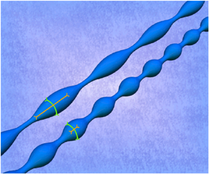
We consider a general complex interface, as sketched in figure 1, which is surrounded by a fluid on both sides. This can either represent the interface of a liquid jet in the co-moving frame or the membrane of a vesicle or biological cell. As usual (Eggers & Villermaux Reference Eggers and Villermaux2008; Boedec et al. Reference Boedec, Jaeger and Leonetti2014), we assume that the interface is infinitely long. In the analytical stability analysis we consider an axisymmetric interface, which is parametrised by the axial position  $z$ and the local radius $R(z,t)$. Initially, the interface is cylindrical with radius $R(z,0)=R_0$. At arbitrary time $t$ the interface is subjected to a perturbation $\delta R(z,t)$, such that the local radius is given by $R(z,t) = R_0 + \delta R(z,t)$.
Illustration of the set-up. We consider a complex interface which can be either a liquid jet of Newtonian fluid in the limit of vanishing viscosity  $\eta$ or the membrane of a vesicle or cell immersed in a fluid in the limit of the Stokes equation, i.e. density $\rho =0$. The fluid jet is immersed in an ambient fluid with $\eta ^0, \rho ^0$. The cylindrical interface of initial radius $R_0$ (dashed line) is subjected to a periodic perturbation with amplitude $\epsilon$ (solid blue line). The interface is parametrised by the position along the cylinder axis $z$ and the radius $R(z,t)$. We consider the interfacial tension in the axial direction $\gamma^z$ (orange) different from that in the azimuthal direction $\gamma^\phi$ (green), both of which contribute to the membrane force acting onto the fluid with different curvature components (grey circles).

In order to perform a linear stability analysis of the complex interface in the presence of anisotropic interfacial tension, we apply a periodic perturbation to its shape (Drazin & Reid Reference Drazin and Reid2004). The perturbation of the interface is illustrated in figure 1: it modulates the radius in  $z$-direction along the cylinder axis with amplitude $\epsilon (t)=\epsilon _0\,{\textrm {e}}^{\omega t}$, a wavelength $\lambda$ and a corresponding wavenumber $k={2{\rm \pi} }/{\lambda }$ of the wave vector pointing along the cylinder axis. The perturbation with initial amplitude $\epsilon _0$ grows in time with growth rate $\omega$. Accordingly, the interface of the jet can be described by its radius as
 \begin{equation} R(z,t)=R_0+\epsilon_0 \exp({\omega t +{\textrm{i}} kz}). \end{equation}
Throughout this work, we consider an anisotropic interfacial tension, i.e. the value of the axial tension differs from the value of the azimuthal tension. This anisotropic tension accounts for two fundamentally different situations. First, in a liquid jet anisotropy can arise, e.g. from covering the interface with passive anisotropic surfactant molecules, thus extending the classical concept of liquid–liquid surface tension to an anisotropic situation. Second, in biological cells or tissue, an active biological machinery, cytoskeletal filaments with motor proteins underlining the plasma membrane, can produce anisotropic tensions at the interface as described in more detail in the Introduction. Due to their usually contractile nature, these active tensions enter the physical equations in the same way as the classical surface tension, despite their fundamentally different origin. In the following, we therefore use the same symbol and refer to both scenarios with the general term interfacial tension.
2.2. Interface coupled to a surrounding fluid
Interfacial tension leads to internal forces being transmitted from the interface to the fluid (Green & Zerna Reference Green and Zerna1954; Barthès-Biesel Reference Barthès-Biesel2016; Salbreux & Jülicher Reference Salbreux and Jülicher2017). In contrast to the classical isotropic Rayleigh–Plateau scenario, we assign anisotropic tension to the interface, i.e. we distinguish between the azimuthal  $\gamma ^{\phi }$ and the axial interfacial tension $\gamma ^{z}$. As sketched in figure 1 the periodic perturbation along the axis changes the curvature of the interface both in the azimuthal and in the axial direction. In azimuthal direction the curvature ${1}/{R_\phi }$ is the inverse of the local radius of the interface $R_\phi =R(z,t)$, where we follow the convention that the curvature of a cylinder is positive. Accordingly, the curvature along the axis is given by the negative second derivative of the radius, ${1}/{R_z} = - R^{\prime \prime }$ such that the curvature is negative at a neck and positive at a bulge (compare figure 1). The derivative $R^{\prime \prime }$ follows directly from (2.1).
The anisotropic tension does not depend on the position along the interface, therefore its derivative vanishes and for a liquid–liquid interface no internal forces tangential to the interface arise (Green & Zerna Reference Green and Zerna1954; Salbreux & Jülicher Reference Salbreux and Jülicher2017). The internal force normal to the interface is given by the interfacial tension components weighted by the corresponding principal curvature. Balance of forces requires that this normal force is in equilibrium with the difference in tractions exerted by the fluids on either side of the interface. Thus, the normal traction jump across the interface  ${\rm \Delta} f^n$ reads
 \begin{equation} \frac{ \gamma^\phi}{R_\phi} + \frac{ \gamma^z}{R_z} = {\rm \Delta} f^n. \end{equation}
The traction jump is given by the projection of the three-dimensional viscous stress tensor of the outer and inner fluid onto the interface normal vector (Chandrasekharaiah & Debnath Reference Chandrasekharaiah and Debnath1994). For an incompressible interface or for negligible viscous effects, i.e. for an ideal fluid, the traction jump is determined by the pressure  $p$ of the fluid. With the normal vector pointing outwards from the interface and considering the outer and inner fluid as incompressible, the traction jump in normal direction is thus given by
 \begin{equation} {\rm \Delta} f^n = -p^{{out}} + p^{{in}} = p (r=R), \end{equation}
with pressures  $p^{{out}}$ and $p^{{in}}$ of the outer and inner fluid, respectively, and $p (r=R)$ denoting the pressure difference at the interface. Together (2.2) and (2.3) lead to
 \begin{equation} \frac{\gamma^\phi}{R_\phi} + \frac{\gamma^z}{R_z}= p (r=R), \end{equation}
for an incompressible interface or an ideal fluid interface. The relation in (2.4) reduces to the classical Young–Laplace equation  ${\gamma }/{R} = p$ in the limit of isotropic surface tension $\gamma =\gamma ^\phi =\gamma ^z$ and vanishing curvature along $z$, i.e. $R_z \rightarrow \infty$. The anisotropic interfacial tension thus leads to a pressure disturbance of the inner fluid, where the two contributions of the interfacial tension are weighted with their respective radii of curvature.
2.3. Fluid dynamics
The motion of the fluid inside and outside the jet is in general described by the Navier–Stokes equation
 \begin{equation} \frac{\partial \boldsymbol{v}}{\partial t}+ \left(\boldsymbol{v} \boldsymbol{\cdot} \boldsymbol{\nabla} \right) \boldsymbol{v} = -\frac{1}{\rho} \boldsymbol{\nabla} p + \nu {\rm \Delta} \boldsymbol{v}, \end{equation}
with the velocity field  $\boldsymbol {v}$, fluid density $\rho$, kinematic viscosity $\nu = {\eta }/{\rho }$ and shear viscosity $\eta$. Density and viscosity of the outer fluid are denoted by $\rho ^o$ and $\eta ^o$, respectively. The fact that the liquid is incompressible, which is true for both the liquid of a jet and the liquid encapsulated in a vesicle, leads furthermore to the continuity equation for the incompressible liquid
 \begin{equation} \boldsymbol{\nabla} \boldsymbol{\cdot} \boldsymbol{v} = 0. \end{equation}
The Navier–Stokes and continuity equations together govern the motion of the fluid.
Besides the well-known Reynolds number  $\textit {Re} = {\rho R_{0} V_{0}}/{\eta }$ with a typical velocity $V_{0}$ and the unperturbed interface radius $R_0$ as the typical length, we use the Ohnesorge number (Eggers & Villermaux Reference Eggers and Villermaux2008), which relates characteristic scales of the interface and the surrounding fluid
 \begin{equation} \textit{Oh} = \frac{\eta}{\sqrt{\rho R_0 \gamma}}. \end{equation}
In our anisotropic scenario with  $\gamma ^{z} \neq \gamma ^{\phi }$ we define two distinct Ohnesorge numbers $\textit {Oh}_z$ and $\textit {Oh}_{\phi }$ for the respective interfacial tensions.
In the limit of small velocities or large viscosity, i.e. the Stokes regime, the Reynolds number approaches zero while the Ohnesorge number becomes large. In this regime, the Navier–Stokes equation can be replaced by the linear Stokes equation
 \begin{equation} 0 = -\boldsymbol{\nabla} p + \eta {\rm \Delta} \boldsymbol{v}. \end{equation}
In the limit of large velocities or small viscosity, i.e. for an ideal fluid, the Reynolds number is larger than one and the Ohnesorge number becomes small. Here, the Euler equation applies
 \begin{equation} \frac{\partial \boldsymbol{v}}{\partial t}+ \left(\boldsymbol{v} \boldsymbol{\cdot} \boldsymbol{\nabla} \right) \boldsymbol{v} = -\frac{1}{\rho} \boldsymbol{\nabla}p. \end{equation}
2.4. Numerical simulations
We aim for a comparison of our main analytical results, the dominant wavelength of the instability and its growth rate presented in §§ 4.1 and 4.3, respectively, with numerical simulations solving the coupled fluid and interface dynamics. The simulations further provide us a glimpse on the nonlinear aspects of the instability dynamics. For a Stokes fluid and an ideal fluid with an outer fluid with the same properties, we perform three-dimensional boundary integral method and lattice-Boltzmann/immersed boundary method simulations, respectively.
2.4.1. Three-dimensional numerical investigation of the instability
We consider a fluid column, the liquid jet, immersed in an ambient fluid. We use fully three-dimensional simulations, thus testing also for non-axisymmetric instabilities triggered by anisotropic interfacial tension (which we did not observe).
The interface encapsulates a Newtonian fluid and is surrounded by another Newtonian fluid of the same density  $\rho ^0 = \rho$ or viscosity $\eta ^0 = \eta$. For the fluid, periodic boundary conditions are chosen in each of the three spatial directions together with a kinematic boundary condition at the interface. Fluid dynamics is either solved by the BIM or the LBM/IBM, as detailed below.
Following the set-up sketched in figure 1, we consider an initially cylindrical interface which is modelled as a thin shell and which we discretise by nodes connected to triangles. Anisotropic tension of the interface is realised using the recently developed and validated computational method for active membranes in flows (Bächer & Gekle Reference Bächer and Gekle2019). This approach can treat both the anisotropic surface tension of a liquid jet in the co-moving frame and the anisotropic active tension of a biological cell cortex on the same footing. To investigate the instability dynamics, we initially apply a small periodic perturbation to the cylindrical interface, as shown in figure 1. From this initial configuration the temporal evolution of the interface and the suspending fluid is solved including a dynamical two way coupling of interface and fluid. The method to determine the dominant wavelength and growth rate is described in appendix A.
2.4.2. Boundary integral method
As the simulation method at zero Reynolds number we use the BIM to solve the fluid dynamics (Pozrikidis Reference Pozrikidis2001; Zhao et al. Reference Zhao, Isfahani, Olson and Freund2010). The BIM solves the Stokes equation in the presence of discretised boundaries based on hydrodynamic Green's functions. It directly solves for the fluid velocity at the nodes of the discretised interface for given interface shape and interfacial force density. As a consequence of using the Stokes equation, in BIM simulations inertial effects are excluded. Neglecting inertial effects corresponds to  $\textit {Re} = 0$ and an Ohnesorge number $\textit {Oh} \rightarrow \infty$. Membrane forces due to interfacial tension are calculated as detailed in Bächer & Gekle (Reference Bächer and Gekle2019). As the interfacial tension in the simulation we use $\gamma ^\phi \approx 10\ \textrm {pN}\ \mathrm {\mu }\textrm {m}^{-1}$, a typical tension expected for blood cells (Dmitrieff et al. Reference Dmitrieff, Alsina, Mathur and Nédélec2017). For details on the implementation of the BIM we refer to Guckenberger & Gekle (Reference Guckenberger and Gekle2018).
As the box size, we consider the length of the cylindrical tube, which is typically 80 times the tube radius, along the axis and ten times the tube radius in lateral directions. A typical discretisation of the interface consists of approximately 17 000 nodes and 32 500 triangles. We do not use periodic boundary conditions for the membrane due to technical issues of the implementation used for BIM simulations. We rather place the outer rings of nodes exactly at the beginning and end of the box, respectively, and fix the nodes by elastic springs. Due to an insufficient number of neighbouring nodes, at the boundary nodes the force from the interfacial tension is not calculated. We note that using this set-up, the fluid encapsulated by the membrane remains inside. For the initial small deformation of the interface we choose the amplitude  $\epsilon _0=0.02$. The fluid viscosity is chosen as $\eta \approx 1.2 \times 10^{-3}$ Pa s. We simulate for approximately 100 time steps with adaptive step size and a total simulation time of approximately 20 ms.
2.4.3. Lattice-Boltzmann/immersed boundary method
As a method to solve fluid dynamics at large/finite Reynolds number, we use the LBM (Aidun & Clausen Reference Aidun and Clausen2010; Krüger et al. Reference Krüger, Kusumaatmaja, Kuzmin, Shardt, Silva and Viggen2016) together with the IBM (Peskin Reference Peskin2002; Mittal & Iaccarino Reference Mittal and Iaccarino2005; Bächer, Schrack & Gekle Reference Bächer, Schrack and Gekle2017; Mountrakis, Lorenz & Hoekstra Reference Mountrakis, Lorenz and Hoekstra2017; Bächer et al. Reference Bächer, Kihm, Schrack, Kaestner, Laschke, Wagner and Gekle2018). Our LBM/IBM is implemented in the software package ESPResSo (Limbach et al. Reference Limbach, Arnold, Mann and Holm2006; Roehm & Arnold Reference Roehm and Arnold2012; Arnold et al. Reference Arnold, Lenz, Kesselheim, Weeber, Fahrenberger, Roehm, Košovan and Holm2013; Weik et al. Reference Weik, Weeber, Szuttor, Breitsprecher, de Graaf, Kuron, Landsgesell, Menke, Sean and Holm2019) and has been extensively validated (Gekle Reference Gekle2016; Guckenberger et al. Reference Guckenberger, Schraml, Chen, Leonetti and Gekle2016; Bächer et al. Reference Bächer, Kihm, Schrack, Kaestner, Laschke, Wagner and Gekle2018; Bächer & Gekle Reference Bächer and Gekle2019).
The LBM solves the fluid dynamics on the basis of the mesoscopic Boltzmann equation and accounts for the fluid dynamics according to the full Navier–Stokes equation. The fluid thus has a finite density, a finite viscosity and, therefore, a finite Ohnesorge number. The fluid is discretised by an Eulerian grid and populations representing the distribution functions for the different velocities are assigned to each fluid node. We here use the D3Q19 velocity set and a typical fluid mesh with dimensions of approximately  $650\times 40\times 40$ with some simulation lattices extending up to $800\times 40\times 40$. A typical simulation runs for 500 000 steps. In the limit of an ideal fluid we choose Ohnesorge numbers in the range of $10^{-3}\text {--}10^{-4}$. Initially, the fluid has zero velocity.
The discretised interface is coupled to the background fluid using the IBM. A typical interface contains 18 240 nodes and 36 480 triangles, has a radius of 6 LBM grid cells and is periodic along the axial direction with an initial perturbation amplitude  $\epsilon _0 = 0.02$ in simulations to determine the dominant wavelength. An additional refined simulation set-up is used for determination of the dominant growth rate, where we simulate one period of the dominant mode with initial perturbation $\epsilon _0 = 0.002$ and increased resolution with a radius of 13 LBM grid cells. Here, a typical fluid lattice consists of $180\times 70\times 70$ nodes and a membrane mesh of 15 416 nodes and 30 832 triangles. We again note that axisymmetry is not imposed and that the simulations are fully three-dimensional. The average distance between two interface nodes is approximately the length of one LBM grid cell. An interface node moves with the local fluid velocity which is interpolated at the node position from the surrounding fluid nodes by an eight-point stencil. The force stemming from the interfacial tension and acting from the membrane onto the fluid at the site of each interface node is transmitted to the fluid by the same eight-point stencil interpolation scheme. Thus, the IBM provides a dynamic two way coupling of membrane and fluid.
3. Dispersion relation for anisotropic interfacial tension
3.1. Anisotropic Rayleigh–Plateau instability for a Stokes fluid
Biological cells as well as their synthetic counterpart (vesicles) are typically a few tens micrometres in size. Therefore, we consider the limit of small Reynolds numbers, i.e.  $\textit {Re} \ll 1$, where the Navier–Stokes equation (2.5), reduces to the linear Stokes equation (2.8) which together with the continuity equation (2.6) describes the fluid behaviour. In the following, we consider identical fluid viscosity inside and outside the vesicle, i.e. $\eta ^o = \eta$. Our aim is to obtain the dispersion relation in the case of anisotropic interfacial tension, which gives the growth rate depending on the wavenumber of the perturbation (2.1). As detailed in appendix B.1 we perform a linear stability analysis and obtain the dispersion relation for a Stokes fluid
 \begin{align} \omega (k) &= \frac{\gamma^\phi}{R_0 \eta} \left( 1 - \frac{\gamma^z}{\gamma^\phi}(R_0k)^2 \right) \left[\vphantom{\frac{kR_0}{2}} \textrm{I}_1(kR_0)\textrm{K}_1(kR_0)\right. \nonumber\\ &\quad \left. + \frac{kR_0}{2} \left( \textrm{I}_1(kR_0)\textrm{K}_0(kR_0) - \textrm{I}_0(kR_0) \textrm{K}_1(kR_0) \right) \right], \end{align}
with  $\textrm {I}_\nu (x), \textrm {K}_\nu (x)$ being the modified Bessel functions of the first and second kind, respectively, and of order $\nu$.
Positive values of  $\omega$ correspond to growing perturbations (2.1), whereas perturbation modes with negative growth rate are dampened. Because of the positive prefactor $\omega _0^{S}={\gamma ^{\phi }}/({R_0\eta })$, which is the inverse of the viscocapillary time based on the azimuthal tension $\gamma ^{\phi }$, and the positive modified Bessel functions for positive $kR_0$, the tension anisotropy determines the range of growing, i.e. unstable, modes. We obtain from (3.1) the range of growing modes for values of $kR_0$ between $-\sqrt {{\gamma ^{\phi }}/{\gamma ^{z}}}$ and $\sqrt {{\gamma ^{\phi }}/{\gamma ^{z}}}$. This range depends on the square root of the anisotropy of the interfacial tension. We recover for isotropic tension $\gamma ^z=\gamma ^\phi =\gamma$ the range of growing wavelengths between $-\sqrt {{\gamma ^{\phi }}/{\gamma ^{z}}} = -1$ and $\sqrt {{\gamma ^{\phi }}/{\gamma ^{z}}} = 1$ as found by Plateau (Reference Plateau1873). So in the case of the classical Rayleigh–Plateau instability, the growing wavelengths do not depend on the interfacial tension $\gamma$ but only on the undisturbed radius $R_0$ of the jet (Drazin & Reid Reference Drazin and Reid2004). Here, in addition the anisotropy of interfacial tension enters as a factor.
We show in figure 2(a) the dispersion relation of the classical Rayleigh–Plateau instability, i.e. for isotropic interfacial tension. The growth rate  $\omega$ is plotted only against positive $kR_0$ due to symmetry. We further distinguish the individual contributions from $\gamma ^\phi$, the first term in (3.1), and from $\gamma ^z$, the second term in (3.1), and plot them in orange and green, respectively, together with the total dispersion relation in blue. It is the interplay of the two contributions of the interfacial tension $\gamma ^z$ and $\gamma ^\phi$ that determines the dispersion relation. The azimuthal tension $\gamma ^{\phi }$, i.e. the first term in (3.1), is positive and thus the system would be unstable against any perturbation with arbitrary wavenumber. However, this is not the case, because this term is balanced by the damping contribution from $\gamma ^z$. Both contributions together determine a finite maximum of the dispersion relation, which corresponds to the dominant mode that grows fastest.
Dispersion relation in the Stokes regime for  $\eta =\eta ^o$. Curves are shown for (a) isotropic interfacial tension ${\gamma ^{z}}/{\gamma ^{\phi }} = 1.0$ and for anisotropic interfacial tension with (b) ${\gamma ^{z}}/{\gamma ^{\phi }} = 0.5$ and (c) ${\gamma ^{z}}/{\gamma ^{\phi }} = 2.0$. We distinguish the contributions from $\gamma ^\phi$ (green) and $\gamma ^z$ (orange). An anisotropic tension strongly alters the range of growing modes and shifts the maximum towards larger $kR_0$ in (b) or smaller $kR_0$ in (c). (d) Dispersion relation for vanishing axial interfacial tension, i.e. $\gamma ^z=0$. The $\gamma ^\phi$ contribution (green) has its maximum at $kR_0=1.59$ in each of the panels, because $\gamma ^\phi$ is kept constant. Thus, although all modes are unstable in (d), in principle, there still exists a well-defined finite dominant wavelength for a Stokes fluid due to fluid stresses.

We now consider an anisotropic interface were the contributions  $\gamma ^\phi$ and $\gamma ^z$ are no longer identical. Their changing ratio leads to a different weighting of the contributions to the dispersion relation (3.1). If the destabilising contribution from $\gamma ^\phi$ rises compared to $\gamma ^z$ as shown in figure 2(b), the range of growing wavelengths increases. On the other hand, if $\gamma ^\phi$ decreases relative to $\gamma ^z$, the range becomes smaller (see figure 2c). Because the destabilising $\gamma ^{\phi }$ contribution reaches a maximum at $kR_0=1.59$ and tends to zero for $kR_0\to \infty$, independent of the anisotropy ratio, also for vanishing $\gamma ^z \rightarrow 0$ a well-defined mode at finite $kR_0$ has the largest growth rate. This is shown by figure 2(d) in the case of $\gamma ^z=0$ with an extended $kR_0$-range on the horizontal axis. In the limit $\gamma ^\phi =0$ all modes are stable. Furthermore, changes in the anisotropy ratio shift the position of the maximum of the dispersion relation. If $\gamma ^\phi >\gamma ^z$ (figure 2b), the position of the maximum of $\omega$ shifts to larger values of $kR_0$, if $\gamma ^\phi <\gamma ^z$ the maximum is found at smaller $kR_0$ as shown in figure 2(c). This means for dominating axial tension $\gamma ^z$ the instability wavelength increases.
3.2. Anisotropic Rayleigh–Plateau instability for an ideal fluid
Performing again a linear stability analysis using the same solution procedure as before, we calculate the dispersion relation for an ideal fluid jet with same density inside and outside the jet as detailed in appendix B.2. We obtain the dispersion relation
 \begin{equation} \omega^2 = \frac{\gamma^\phi}{\rho R_0^3} (kR_0)^2 \left( 1 - \frac{\gamma^z}{\gamma^\phi} (kR_0)^2 \right) \textrm{I}_1(kR_0) \textrm{K}_1(kR_0). \end{equation}
 Compared to the dispersion relation for a Stokes fluid in (3.1), we here obtain an equation for the squared growth rate  $\omega ^2$. According to the ansatz for the perturbed interface in (2.1), perturbations with real and positive $\omega$ will grow. Imaginary $\omega$ describe oscillatory perturbations of the surface which do not grow in time. Imaginary $\omega$ correspond to negative values of $\omega ^2$. Each positive $\omega ^2$ has a positive and negative solution $\omega$. The positive solution will grow while the negative is damped. Thus, we are interested in non-negative values of $\omega ^2$ which are obtained from (3.2). This leads to the same expression for the range of growing wavelengths as for the Stokes fluid in § 3.1 because the relevant factor in the dispersion relation is identical, i.e. the anisotropy ratio ${\gamma ^{z}}/{\gamma ^{\phi }}$ enters the equation in the same way. However, the prefactor of the growth rate changes $\omega _0^2 = {\gamma ^{\phi }}/({\rho R_0^3})$, it now depends on the density rather than on the viscosity and is the squared inverse of the capillary time based on the azimuthal tension $\gamma ^\phi$. Furthermore, the geometrical factor containing the Bessel functions is remarkably different.
The dispersion relation (3.2) for the ideal fluid is shown in figure 3(a–c) for same values of the anisotropy ratio as in figure 2(a–c). We again observe a strong variation of the maximum position and range of unstable modes with changing anisotropy ratio. A remarkable difference to the Stokes fluid is the shape of the  $\gamma ^{\phi }$ contribution. Here for an ideal fluid the destabilising $\gamma ^{\phi }$ contribution no longer reaches a maximum at finite $kR_0$ but instead increases indefinitely. Thus, in the limit $\gamma ^z=0$ all modes are unstable with steadily increasing growth rate. Compared to the Stokes fluid, the total dispersion relation is furthermore more asymmetric between $kR_0 = 0$ and $\sqrt {{\gamma ^{\phi }}/{\gamma ^{z}}}$ and the maximum shifts towards larger wavenumbers (compare e.g. figure 2b to figure 3b).
Dispersion relation for an ideal fluid with  $\rho =\rho ^o$. Curves are shown for (a) isotropic interfacial tension ${\gamma ^z}/{\gamma ^\phi } = 1.0$ and for anisotropic interfacial tension with (b) ${\gamma ^z}/{\gamma ^\phi } = 0.5$ and (c) ${\gamma ^z}/{\gamma ^\phi } = 2.0$. We distinguish the contributions from $\gamma ^\phi$ (green) and $\gamma ^z$ (orange). While $\gamma ^z$ is purely damping, $\gamma ^\phi$ is destabilising. An anisotropic tension strongly alters the range of growing modes and shifts the maximum towards larger $kR_0$ in (b) or smaller $kR_0$ in (c).

In appendix E we further generalise our results to the dispersion relation including a general density and viscosity contrast as derived by Tomotika (Reference Tomotika1935).
4. Quantitative analysis of the effects due to tension anisotropy
4.1. Dominant wavelength
Having determined the range of (un)stable wavenumbers in the previous section, we now explicitly investigate how tension anisotropy affects the value of the dominant, i.e. fastest growing, wavelength  $\lambda _{m}$. This quantity is of practical interest as it determines the size of the fragmented vesicles/droplets and provides an intrinsic length scale of the instability. For arbitrary ratios ${\gamma ^{z}}/{\gamma ^{\phi }}$, we use Mathematica to determine numerically the maximum of the dispersion relation (3.1) and (3.2). We further perform fully three-dimensional simulations of a membrane endowed with interfacial tension using BIM and LBM/IBM, as detailed in § 2.4. While BIM intrinsically solves the fluid dynamics in the Stokes limit, LBM/IBM simulations are run for $\textit {Oh} \approx 0.00025$, i.e. very close to the ideal fluid limit.
The result of the linear stability analysis is compared to the simulation results in figure 4. The solid lines show how the position of the maximum of the dispersion relations (3.1) (orange line in figure 4a) and (3.2) (red line in figure 4b), i.e. the dominant wavelength  $\lambda _{m}$, changes with the ratio ${\gamma ^{z}}/{\gamma ^{\phi }}$. The simulation results for the Stokes fluid using BIM are drawn as triangles, those for the ideal fluid using LBM/IBM as squares. Both are in very good agreement with the respective theoretical predictions. For the Stokes fluid the obtained value $k_m R_{0} \approx 0.562$ (i.e. ${\lambda _m}/{R_0} \approx 11.18$) for isotropic tension ${\gamma ^{z}}/{\gamma ^{\phi }}=1$ is in good agreement with Tomotika (Reference Tomotika1935) and Stone & Brenner (Reference Stone and Brenner1996). For the ideal fluid the dominant wavelength is smaller compared to the Stokes limit, which is true for all values of $kR_0$. For both Stokes fluid and ideal fluid increasing the ratio ${\gamma ^{z}}/{\gamma ^{\phi }}$ leads to an increase in the wavelength compared to its value at isotropic tension (illustrated by the insets from simulations on the right-hand sides of figures 4a and 4b). For decreasing ratio the opposite happens, the wavelength decreases (see inset from simulations at the top of figures 4a and 4b). Over the entire range of interfacial tension ratios we observe a nonlinear dependence of the wavelength on the anisotropy ratio. In the Stokes regime at an anisotropy ratio of zero a finite wavelength dominates. This is due to the fact that the $\gamma ^{\phi }$-contribution to the dispersion relation, as shown in figure 2(d), does not diverge for large wavenumbers but rather has a maximum at $k_m R_0=1.59$ which corresponds to a wavelength of $\lambda _m = 3.96 R_0$. This value matches the $y$-axis intercept of the dominant wavelength in figure 4(b). For the ideal fluid, however, for vanishing anisotropy ratio the wavelength goes to zero. In the limit of infinite ratio the wavelengths tend to infinity for both Stokes and ideal fluid.
Dominant wavelength as function of the anisotropy in interfacial tension. (a) Simulation results from BIM for the Stokes fluid are in very good agreement with the analytical results obtained from the dispersion relation (3.1). (b) Results for the ideal fluid from LBM/IBM agree very well with dominant wavelength obtained from the analytical dispersion relation (3.2). While the whole curve is at larger values in the Stokes limit, in both cases the dominant wavelength increases steadily with increasing  ${\gamma ^z}/{\gamma ^\phi }$. Simulation snapshots of the interface are shown for different ratios ${\gamma ^{z}}/{\gamma ^{\phi }}$ over a length of about $55 R_0$ as insets.

In order to explain the effect of anisotropic interfacial tension, we first recall the classical Rayleigh–Plateau mechanism where two opposing effects influence the break-up. Since the radius in the region of a constriction is smaller than in a peak region, a pressure gradient develops pushing fluid out of the constriction and thus amplifying the disturbance. At the same time, however, due to the perturbation of the surface, the radius of curvature along the  $z$-direction is negative in the region of the constriction and positive in the region of a peak. As can be seen from the Young–Laplace equation (2.4) this introduces another pressure gradient dragging the liquid back from the peak regions thus counteracting the pressure difference due to variations of the radius. The instability is a result of the interplay of both effects. An anisotropic interfacial tension weights these effects by either the azimuthal tension $\gamma ^\phi$ or axial tension $\gamma ^z$. Thus, a change in the ratio of the interfacial tension leads to a change in the weighting, shifting the region of growing wavelength and also altering the most unstable wavelength. This argument is illustrated by the three cases of the dispersion relation with its different contributions shown in figures 2 and 3.
The limit  $\lambda _{m}\rightarrow \infty$ for $\gamma ^z \rightarrow \infty$ can be understood on the basis of the Young–Laplace equation for anisotropic interfacial tension in (2.4), as well. For infinite $\gamma ^z$ a finite curvature along $z$ would result in an infinite pressure difference. Thus, the interfacial tension must be balanced by a vanishing curvature, i.e. by an infinite curvature radius, which is equivalent to an infinite wavelength.
Finally, we discuss the limit  $\gamma ^z\rightarrow 0$. We start with considering the ideal fluid. Due to finite $\gamma ^\phi$ every circular segment of the interface along the cylinder axis tends to contract. The incompressibility of the liquid inside prevents this homogeneous contraction. This means that a volume conserving neck–tail perturbation between two neighbouring thin circular segments, thus with very small wavelength and very large curvature in the $z$-direction, can in principle be established. Since $\gamma ^z\rightarrow 0$ there is no counteracting contribution which balances this tendency. The monotonic increase of the growth rate for the $\gamma ^\phi$-contribution with increasing $k$, as shown by the course of the dispersion relation in figure 3, suggests that such a perturbation grows fastest. This, in total, results in $\lambda _{m} \rightarrow 0$ for the ideal fluid. In the Stokes limit, however, the $\gamma ^{\phi }$-contribution is finite for large $kR_0$, possibly due to viscous stresses from the fluid which have a damping effect on the perturbation.
4.2. Transition between the two regimes
In the following, we will show that the border between the Stokes regime and the ideal fluid limit is not necessarily clear cut. In fact, by varying nothing more than the anisotropy ratio, the system can undergo a transition from one regime to the other. To demonstrate this transition, we present simulations using the LBM/IBM for typical parameters of biological cells/vesicles. We choose an interfacial tension of  $\gamma ^{\phi } = 10^{-4}\ \textrm {N}\ \textrm {m}^{-1}$, which is the cortical tension reported for neutrophils (Tinevez et al. Reference Tinevez, Schulze, Salbreux, Roensch, Joanny and Paluch2009) and in the middle of the range of typical tensions reported by Winklbauer (Reference Winklbauer2015). As typical diameter of the tubular vesicle we choose $2R_0 = 1\ \mathrm {\mu }\textrm {m}$ and for the surrounding fluid density $\rho =1000\ \textrm {kg}\ \textrm {m}^{-3}$ and viscosity $\eta =1.2\times 10^{-3}\ \textrm {Pa}\ \textrm {s}$.
The dominant wavelength is shown in figure 5(a) as a function of the anisotropy ratio with green dots. For a clear comparison we also show the Stokes fluid dispersion relation in orange and the relation for the ideal fluid in red. The numerical simulations exhibit a transition between the two curves. For a small anisotropy ratio we obtain a finite wavelength, which nearly matches the result in the Stokes regime. In the case of isotropic tension we obtain a dominant wavelength of  $k_m R_{0} \approx 0.628$ (i.e. ${\lambda _{m}}/{R_0} \approx 10.005$), a value in between the one for the ideal fluid and the Stokes regime. For larger values of the anisotropy ratio we end up close to the curve for an ideal fluid.
Transition between both regimes. (a) LBM/IBM simulations with typical vesicle and cell parameters (green dots) show dominant wavelengths between the two curves obtained in the limit of a Stokes fluid (orange) and an ideal fluid (red). (b) The transition between the two regimes in the wavelength is accompanied by a strong variation in the Ohnesorge number with respect to the tension along the axis  $z$, i.e. $\textit {Oh}_z$.

We explain the transition between both regimes by the varying Ohnesorge number, which is shown in figure 5(b). By varying the anisotropy ratio, either the Ohnesorge number  $\textit {Oh}_{\phi }$ or $\textit {Oh}_{z}$ varies, while the other can be kept constant. Here, we keep $\textit {Oh}_{\phi } \approx 5.5$ shown by the dark-green downwards-pointing triangles in figure 5(b). Consequently, $\textit {Oh}_{z}$ changes from 30 to approximately 2.5, as shown by the light-green upwards-pointing triangles. The transition in the Ohnesorge number $\textit {Oh}_{z}$ is matched by the transition in the wavelength. At small anisotropy ratios with large Ohnesorge number, the wavelength is close to the analytical prediction for the Stokes equation. This is in good agreement with the Stokes equation having $\textit {Oh} \rightarrow \infty$. Towards larger anisotropy ratios the Ohnesorge number becomes smaller and the wavelength approaches the predictions for an ideal fluid. We thus conclude that finite inertia effects trigger the transition, even though the Ohnesorge number is still larger than one. Our results clearly show that finite inertia effects can alter the Rayleigh–Plateau instability of tubular vesicles, even though their micrometric dimensions may at first sight suggest the opposite.
4.3. Dominant growth rate
We now investigate the growth rate of the most unstable mode  $\omega _{m}$, i.e. the value of the maximum of the dispersion relation, in a quantitative manner. Using Mathematica we determine the maximum growth rate for varying tension anisotropy from the analytical dispersion relation. In addition, we perform simulations as described in § 2.4, where we extract the growth rate as described in appendix A.
The results in the limit of a Stokes fluid are shown in figure 6(a) and the limit of an ideal fluid is shown in figure 6(b). With increasing tension anisotropy the dominant growth rate decreases strongly. This can again be explained by the stabilising nature of the axial tension  $\gamma ^z$ which slows down the instability. For tension anisotropy approaching infinity the growth rate approaches zero. At tension anisotropy equal zero we observe a finite growth rate of $\omega _{m} \approx 0.087$ for the Stokes fluid in (a), which results from viscous stresses in the Stokes fluid. In stark contrast, for an ideal fluid in (b) the maximum growth rate increases more strongly and even diverges for tension anisotropy to zero due to the destabilising nature of the azimuthal tension $\gamma ^{\phi }$. Simulation results for the Stokes fluid with BIM (triangles) and for the ideal fluid with LBM/IBM (squares) are in very good agreement with the corresponding analytical results. From the inverse of the growth rate the linear break-up time can be estimated, which is the time it takes until a droplet or vesicle pinches off. From figure 6 we can conclude that with decreasing tension anisotropy the break-up of the interface is strongly accelerated.
Growth rate of the dominant mode as a function of the anisotropy in interfacial tension. The dominant growth rate according to the dispersion relation (a) for a Stokes fluid (3.1) (orange line) and (b) for an ideal fluid (3.2) (red line) is shown with corresponding BIM simulations (triangles) and LBM/IBM simulations (squares), respectively, depending on the tension anisotropy  ${\gamma ^z}/{\gamma ^\phi }$. The dominant growth rate decreases steadily and strongly with increasing tension anisotropy. While the decrease with increasing anisotropy is similar, the growth rate is one order of magnitude larger for the ideal fluid and it does not remain finite at zero anisotropy in contrast to the Stokes fluid in (a). In both cases simulation results are in perfect agreement with the theory.

4.4. Nonlinear correction to the linear break-up time
After discussing dispersion relation, growth rate and dominant wavelength obtained by linear stability analysis, we now proceed to investigate the nonlinear behaviour of the Rayleigh–Plateau instability. This is covered by the simulations presented above using BIM for a Stokes fluid and LBM/IBM for an ideal fluid. In the following, we extract the nonlinear correction of the linear break-up time (Ashgriz & Mashayek Reference Ashgriz and Mashayek1995; Martínez-Calvo et al. Reference Martínez-Calvo, Rivero-Rodríguez, Scheid and Sevilla2020), which we define based on (A 1) by
 \begin{equation} {\rm \Delta} t_{nl} = t_{b} - \frac{\ln(\epsilon_0^{-1})}{\omega_{m}}, \end{equation}
from simulations with initial perturbation amplitude  $\epsilon _0$ as described in appendix A. This correction compares the break-up time obtained from simulations $t_{b}$ to the linear break-up time obtained from the maximum growth rate of the dispersion relation $\omega _{m}$ and is shown in figure 7 in relation to $t_{b}$. In the limit of a Stokes fluid the nonlinear correction varies strongly: we observe a change of sign above an anisotropy ratio of about ${\gamma ^z}/{\gamma ^\phi }=0.5$ where the correction becomes strongly negative. The nonlinear correction for the ideal fluid for the LBM/IBM is smaller, positive, and slightly increases with increasing tension anisotropy. For isotropic tension but varying Marangoni number of a surfactant-covered fluid jet Martínez-Calvo et al. (Reference Martínez-Calvo, Rivero-Rodríguez, Scheid and Sevilla2020) report effects going in the same direction with a more pronounced variation of the nonlinear correction of the linear break-up time towards the Stokes limit and less variation towards the ideal fluid limit.
Nonlinear correction of the linear break-up time for varying tension anisotropy. The nonlinear correction of the linear break-up time is shown relative to the break-up time  $t_{b}$ obtained from simulations. In the limit of an ideal fluid the LBM/IBM simulations show a slightly increasing nonlinear correction to the linear break-up time with increasing tension anisotropy. In contrast, BIM simulations show the reversed behaviour for a Stokes fluid, where in addition the sign changes and the amplitude variations are more pronounced.

5. Influence of interface viscosity
We now investigate how anisotropic interfacial tension influences the instability wavelength and growth rate in the Stokes regime if the interface in addition possesses interface viscosity (Boussinesq Reference Boussinesq1913; Scriven Reference Scriven1960; Whitaker Reference Whitaker1976; Hajiloo, Ramamohan & Slattery Reference Hajiloo, Ramamohan and Slattery1987; Powers Reference Powers2010; Yazdani & Bagchi Reference Yazdani and Bagchi2013; Narsimhan et al. Reference Narsimhan, Spann and Shaqfeh2015; Martínez-Calvo & Sevilla Reference Martínez-Calvo and Sevilla2018; Guglietta et al. Reference Guglietta, Behr, Biferale, Falcucci and Sbragaglia2020). The dispersion relation in presence of interface viscosity and tension anisotropy is derived in appendix B.3 and reads
 \begin{align} \omega &= \frac{\gamma^\phi}{\eta R_0} \left(1 - \frac{\gamma^z}{\gamma^\phi} (kR_0)^2 \right) \left( 1+ \frac{2\eta_{S}}{\eta R_0} kR_0 \xi \right)^{-1} \left[\vphantom{\frac{kR_0}{2}} {\rm I}_1(kR_0){\rm K}_1(kR_0) \right. \nonumber\\ &\left.\quad + \frac{kR_0}{2}\left( {\rm I}_1(kR_0) {\rm K}_0(kR_0) - {\rm I}_0(kR_0) {\rm K}_1(kR_0) \right)\right] \end{align}
with the abbreviation
 \begin{equation} \xi = - \tfrac{1}{2} \left[ kR_0 {\rm I}_1 (kR_0){\rm K}_1(kR_0) - kR_0 {\rm I}_0(kR_0) {\rm K}_0(kR_0) \right]. \end{equation}
For vanishing interface viscosity  $\eta _{S}$ the dispersion relation correctly reduces to (3.1).
From the dispersion relation we numerically calculate the dominant wavelength  $\lambda _{m}$ and the corresponding growth rate $\omega _{m}$ for varying anisotropy ratio ${\gamma ^z}/{\gamma ^\phi }$ and interface viscosity $\eta _{S}$, which we measure relative to fluid viscosity $\eta$. Phase diagrams of the dominant wavelength and the corresponding growth rate are shown in figures 8(a) and 8(b), respectively. Typical values for the interface viscosity of vesicles and red blood cells reported in the literature vary from $10^{-10}$ Pa s m to $10^{-7}$ Pa s m (Dimova et al. Reference Dimova, Aranda, Bezlyepkina, Nikolov, Riske and Lipowsky2006; den Otter & Shkulipa Reference den Otter and Shkulipa2007; Guglietta et al. Reference Guglietta, Behr, Biferale, Falcucci and Sbragaglia2020). In combination with typical fluid viscosities (§ 2.4) and sizes of the order of $R_0=1\ \mathrm {\mu }\mathrm {m}$ for vesicles and $R_0=4\ \mathrm {\mu }\mathrm {m}$ for red blood cells this leads to typical viscosity ratios ${2\eta _{{S}}}/({\eta R_0}) = 0.1 \text {--} 40$. In figure 8 these values correspond to the range from approximately $-1$ to approximately 1.6 on the ordinate. For fixed values of the viscosity ratio, an increase in the anisotropy ratio leads to a larger dominant wavelength and smaller maximum growth rate. This is in line with the results discussed above for zero interface viscosity in §§ 4.1 and 4.3. Especially in the region of small interface viscosities, changes in $\eta _{S}$ have little effect on dominant wavelength and growth rate, but also around a fraction of 1 the anisotropy dominates. If the interface viscosity $\eta _{S}$ becomes very large compared to the fluid viscosity, the growth rate tends to zero, as a more viscous interface leads to a slower dynamics of the perturbation. The latter is consistent with the results of Narsimhan et al. (Reference Narsimhan, Spann and Shaqfeh2015) for isotropic interfaces. We also note that the maximum wavenumber of the instability, beyond which perturbations do not grow, is influenced only by the anisotropy ratio and not the viscosity ratio, because the root of the dispersion relation (5.1) is determined by the first term in brackets.
Influence of interface viscosity on the anisotropic Rayleigh–Plateau instability. Phase diagrams for (a) the dominant wavelength and (b) the corresponding growth rate. The dominant wavelength increases both with increasing anisotropy ratio and increasing interface viscosity  $\eta _{S}$. The growth rate of the dominant perturbation decreases with increasing anisotropy ratio and interface viscosity. Despite the increase in the wavelength and the slowing down of the instability for very large values of the interface viscosity, the tension anisotropy is the dominating parameter.

6. Formation of satellite droplets for an ideal fluid jet without ambient fluid under influence of tension anisotropy
We eventually consider an ideal fluid jet without ambient fluid, i.e.  $\eta ^0 = 0$ and $\rho ^0 \ll \rho$. In appendix C we derive the dispersion relation including anisotropic interfacial tension and show that for the ideal fluid jet without ambient fluid similar results hold as for the ideal fluid discussed in §§ 3.2 and 4. To compare our analytical results to simulations of an ideal fluid jet without ambient fluid we develop an axisymmetric simulation method based on a long-wavelength (or small- $k$) approximation as detailed in appendix D. We consider the Navier–Stokes equation (D 9) together with the kinematic boundary condition (D 10) in the small- $k$ approximation and solve them numerically. From the dynamic evolution the dominant growth rate and wavelength can be calculated, similarly to the procedure for the three-dimensional simulations detailed in appendix A. They are in good agreement with the theory as detailed in appendix C. We further obtain the jet shape over time.
With this, we are able to study the formation of satellite droplets under anisotropic interfacial tension. Satellite droplets are typically much smaller than and form in between the main drops during break-up of a liquid jet for certain parameter combinations (Eggers & Dupont Reference Eggers and Dupont1994; Eggers Reference Eggers1997; Martínez-Calvo et al. Reference Martínez-Calvo, Rivero-Rodríguez, Scheid and Sevilla2020). In the presence of an ambient fluid (BIM and LBM/IBM simulations) we do not observe satellite droplet formation, which may be related to limitations in the resolution of our simulation and the fact that we do not simulate the actual pinch-off. In the following, we therefore investigate satellite droplet formation using the small- $k$ simulations for a liquid jet without ambient fluid at varying tension anisotropy and viscosity. Starting with the zero-viscosity, ideal fluid jet ( $Oh=0$), we observe satellite droplets as shown at the bottom of figure 9. As the dominant wavelength increases with increasing anisotropy, the satellite droplet at the bottom right of figure 9 is more elongated compared to the left one. However, both satellites possess the same relative volume of approximately $\varXi =3$ % (Rutland & Jameson Reference Rutland and Jameson1970; Lafrance Reference Lafrance1975; Mansour & Lundgren Reference Mansour and Lundgren1990; Ashgriz & Mashayek Reference Ashgriz and Mashayek1995; Eggers Reference Eggers1997), which is defined as the volume integral over the satellite droplet divided by the volume integral over one period of the perturbation (Martínez-Calvo et al. Reference Martínez-Calvo, Rivero-Rodríguez, Scheid and Sevilla2020). For the ideal fluid jet, $\varXi$ is independent of the tension anisotropy.
Formation of satellite droplets under the influence of tension anisotropy in the absence of an ambient fluid  $\rho ^o=0, \eta ^o=0$. Relative volume $\varXi$ of the satellite droplet for varying tension anisotropy ${\gamma ^z}/{\gamma ^\phi }$ and varying Ohnesorge number $Oh$. Parameter combinations for the shapes shown around the colour map are indicated in the phase diagram by black crosses. For the ideal fluid jet without ambient fluid with $\rho ^o=0$ ( $Oh=0$) the relative volume of 3 % remains constant while for the Stokes fluid without ambient fluid $\eta ^o = 0$ (large $Oh$) no satellites appear. In the intermediate range, a significant influence of tension anisotropy on the relative volume is observed. Especially, the satellite droplet becomes cylindrical for large tension anisotropy, as shown in the top right image.

As our small- $k$ simulations are based on the full Navier–Stokes equation, they allow us to explore the effect of fluid viscosity measured in terms of the Ohnesorge number $Oh$ on the satellite droplet. In the centre of figure 9 we show the relative volume $\varXi$ in a colour map. For isotropic interfacial tension, we observe a decrease in the satellite volume, which is in agreement with results reported by Martínez-Calvo et al. (Reference Martínez-Calvo, Rivero-Rodríguez, Scheid and Sevilla2020) in the absence of surfactants. With increasing Ohnesorge number the phase diagram in figure 9 shows a growing influence of the anisotropy. For a small but non-zero $Oh\approx 0.2$, the volume assumes its maximum at ${\gamma ^z}/{\gamma ^\phi }=0$ and decreases with increasing anisotropy. At higher $Oh$, the effect is reversed and the volume strongly increases with increasing tension anisotropy. In contrast to $Oh=0$, at larger Ohnesorge number $Oh=0.9$ the shape of the satellite droplet is strongly influenced by an increase in tension anisotropy from ${\gamma ^z}/{\gamma ^\phi }=0.5$ to ${\gamma ^z}/{\gamma ^\phi }=3.5$ as illustrated by the images at the top of figure 9. For small anisotropy (upper left shape) the satellite droplet is small and spherical but most remarkably for larger tension anisotropy (upper right) it develops a more cylindrical shape, it is longer and larger. In both cases the satellite droplet is connected to the main droplets by a thin fluid string. At very large Ohnesorge number beyond one, i.e. towards the Stokes regime, the satellite volume decreases to zero over the whole range of anisotropy. All in all, over a broad range of intermediate Ohnesorge numbers we observe a striking influence of tension anisotropy on the satellite droplet, where at larger $Oh$ larger tension anisotropy stabilises the satellite droplet.
7. Conclusion
Using linear stability analysis supported by numerical simulations we generalised the Rayleigh–Plateau mechanism for the break-up of a liquid cylinder to situations where the interfacial tension is anisotropic. Two physically relevant situations were studied: a vesicle/biological cell in the limit of small Reynolds number (Stokes equation) and an ideal fluid in the limit of large Reynolds number (Euler equation). We found that anisotropic interfacial tension alters not only the range of growing perturbations but also strongly affects the dominant wavelength of the instability. If the axial tension is inferior/superior to the azimuthal tension, the dominant wavelength becomes smaller/larger than the wavelength of the classical isotropic Rayleigh–Plateau instability. For strong anisotropy, the dominant wavelength can even lie outside the instability range of the classical isotropic Rayleigh–Plateau instability. The predictions of our linear stability analysis were found to be in excellent agreement with numerical simulations using a boundary integral method at low and a lattice-Boltzmann/immersed boundary method at high Reynolds number. LBM/IBM simulations with typical vesicle/cell parameters, which include finite inertia effects, show a transition in the wavelength for decreasing Ohnesorge number from the Stokes regime to the ideal fluid. Using simulations, we found the nonlinear correction to the linear break-up time to decrease/increase with the anisotropy ratio in the Stokes/Euler limits, respectively. We found that including viscosity of the interface surrounded by Stokes fluid leads to an increase in the dominant wavelength and a slower dynamics of the perturbation. However, except at very large interface viscosity, changes are small compared to the effects of varying tension anisotropy. Finally, we showed that the satellite droplet volume of 3 % is not affected by varying tension anisotropy in the limit of an ideal fluid. For Ohnesorge numbers just below one, the satellite volume decreases with increasing anisotropy.
In Reference Bächer, Graessel and GeklePart 2 we investigate the alteration of the anisotropic Rayleigh–Plateau instability due to the bending and shear elasticity present in a typical cell. Besides biological cells, our results apply to synthetic interfaces with anisotropic properties such as nematic liquid crystals confined to interfaces (Keber et al. Reference Keber, Loiseau, Sanchez, DeCamp, Giomi, Bowick, Marchetti, Dogic and Bausch2014) or cell-laden hydrogels extruded from a nozzle during bioprinting applications (Snyder et al. Reference Snyder, Rin Son, Hamid, Wang, Lui and Sun2015; Mandrycky et al. Reference Mandrycky, Wang, Kim and Kim2016).
Acknowledgements
C.B. and K.G. thank the Studienstiftung des deutschen Volkes for financial support. C.B. acknowledges support by the study programme ‘Biological Physics’ of the Elite Network of Bavaria. We acknowledge funding from Deutsche Forschungsgemeinschaft in the framework of FOR 2688 ‘Instabilities, Bifurcations and Migration in Pulsating Flow’, Project B3. We gratefully acknowledge computing time provided by the SuperMUC system of the Leibniz Rechenzentrum, Garching, as well as by the Bavarian Polymer Institute, and financial support from the Volkswagen Foundation.
Declaration of interests
The authors report no conflict of interest.
Appendix A. Simulation analysis
In the following we explain in detail the analysis procedure of the BIM and LBM/IBM simulations. In order to analyse in simulations both the wavelength of the dominant mode and its growth rate we consider the interface shape over time for a given perturbation and track a local maximum corresponding to a later droplet/vesicle as shown in figure 10(a). In order to obtain the most unstable mode for given anisotropic interfacial tension in the simulations, we consider a cylindrical interface of fixed anisotropic interfacial tension immersed in a fluid of fixed properties and apply a series of perturbations with varying wavelength. One simulation corresponds to one perturbation with fixed wavelength. The initial amplitude of the perturbation is chosen as  $\epsilon (t=0) = 0.02 R_0$ in all simulations. Note that a multiple of the wavelength has to fit in the simulation box and we thus vary the wavelength in discrete steps. Figure 10(a) shows an example of a series of simulations for given anisotropic interfacial tension ${\gamma ^z}/{\gamma ^\phi } = 0.4$ using the LBM/IBM. In this example we force a perturbation with 10–17 maxima onto a cylindrical interface in a box of length 650 grid cells. Each curve corresponds to a simulation with different wavelength of the perturbation. In each of the simulations the radius at the position of the different maxima is tracked over time. The curves show the local radius at the position of the maxima, averaged over all maxima, varying in time. From the initial amplitude $\epsilon (t=0) = 0.02 R_0$ all modes grow with a different speed. In order to determine the fastest growing wavelength, we define a threshold for the amplitude $\epsilon _{{crit}}= 0.1 R_0$, which can be considered as an upper limit of small deformations. The inset of figure 10 shows the growth of all modes up to the radius $R_0 + \epsilon _{{crit}}$. The mode which first reaches this threshold, is considered as the fastest growing mode and its corresponding wavelength as the most unstable wavelength. This procedure can be applied to different values of the anisotropy ratio ${\gamma ^z}/{\gamma ^\phi }$ and allows us to numerically determine the most unstable wavelength depending on tension anisotropy. With increasing wavelength we increase the box length in order to ensure a good resolution for this procedure. Nevertheless, the finite box size and the resulting discrete variation of the wavelength result in discretisation effects. In order to account for these discretisation effects we compute the range in wavelength which cannot be distinguished due to the discrete variation: adding/subtracting half the wavelength is not possible for a given box length, because we necessarily enforce an integral number of wavelengths in the simulation box. This range is given in the figures as error bars of the simulation results.
Illustration of the analysis of the numerical simulations. (a) For fixed values of the anisotropic interfacial tension, in this case  ${\gamma ^z}/{ \gamma ^\phi }= 0.4$, we run multiple simulations with varying wavelengths of the interface perturbation. One simulation corresponds to one wavelength, which is determined by the number of maxima (different curves) per box length. The radius averaged over all maxima divided by the unperturbed radius $R_0$ is shown over time. The inset shows the growth up to a radius of 110 % of $R_0$. The first simulation to reach this threshold is considered as the fastest growing mode. (b) LBM/IBM simulations of a single period of the perturbation with increasing resolution and smaller initial perturbation amplitude $\epsilon _0 = 0.002$ allow us to determine the growth rate (here shown for different perturbation wavelengths with ${\gamma ^z}/{\gamma ^\phi } = 2$ in comparison to the analytical solution (3.2)) and the nonlinear correction of the linear break-up time.

The growth rate is calculated as the quotient of the derivative of the maximum radius over time and the maximum radius itself, in a regime of linear growth. In BIM simulations we use the series of perturbations as detailed above, for the LBM/IBM simulations we consider one period of the dominant perturbation with increased resolution and initial perturbation amplitude  $\epsilon _0 = 0.002$. Figure 10(b) shows the growth rate determined from simulations for varying wavenumber in comparison to the analytically obtained dispersion relation (3.2) for LBM/IBM simulations. An error is estimated from the average value of the quotient which determines the growth rate.
As a measure of the nonlinear behaviour covered by the simulations, we further extract the nonlinear correction to the linear break-up time  ${\rm \Delta} t_{nl}$ defined in (4.1). To do so we determine the break-up time in the simulation $t_{b}$ by tracking a minimum of the interface shape over time and extrapolating the last time steps towards a radius of zero. From the analytical evolution of a perturbation based on the linear stability analysis as given in (B 1) the linear break-up time can be calculated at the position of a minimum by
 \begin{equation} R_{{min}} = R_0 - R_0 \epsilon_0 \,\mathrm{e}^{\omega t} \stackrel{!}{=} 0. \end{equation}
The difference between  $t_\mathrm {b}$ and the linear break-up time determines the nonlinear correction as given by (4.1).
Appendix B. Analytical derivation of the dispersion relations
B.1. Dispersion relation for a Stokes fluid
In the following we consider the inner and outer fluid in the Stokes limit with same viscosity, i.e.  $\eta ^o = \eta$. The following calculations are based on the method introduced by Stone & Brenner (Reference Stone and Brenner1996). We use an ansatz of a cylindrical interface which is slightly perturbed in a periodic fashion with time dependent amplitude $\epsilon (t)\ll 1$. For later convenience we write the equation describing the shape as
 \begin{equation} R = R_0 \left( 1 + \epsilon(t) \cos (kz) \right), \end{equation}
which is a slightly different notation but equivalent to the ansatz in (2.1). We calculate the traction jump at the interface  ${\rm \Delta} f_n$ in (2.2), which is equal to the negative membrane force, using (B 1) and assuming that the magnitude of the interface perturbation is small, i.e. $\epsilon \ll 1$,
 \begin{equation} \frac{\gamma^{\phi}}{R(z,t)}+\frac{\gamma^{z}}{R_z(z,t)}\approx \frac{\gamma^{\phi}}{R_0}\left(1\!-{\epsilon} \cos (kz) \right)\!-\!\gamma^{z}\frac{\partial^2 R}{\partial z^2} = \frac{\gamma^{\phi}}{R_0} \left(1\!-\! \left[ 1 - \frac{\gamma^z}{\gamma^\phi} (kR_0)^2 \right] \epsilon \cos (kz) \right)\!. \end{equation}
The traction jump can be decomposed into a constant pressure contribution  $p_0={\gamma ^\phi }/{R_0}$ and a perturbation in the traction jump
 \begin{equation} -\frac{\gamma^\phi}{R_0} \epsilon \left( 1-\frac{\gamma^z}{\gamma^\phi} (R_0k)^2 \right) \cos(kz), \end{equation}
which is evaluated at the position of the unperturbed interface due to linearisation (Tomotika Reference Tomotika1935; Stone & Brenner Reference Stone and Brenner1996). The goal now is to solve the Stokes equation (2.8) in the presence of the traction jump perturbation (B 3). This is done by considering a ring force representing the traction jump (Stone & Brenner Reference Stone and Brenner1996) such that the Stokes equation becomes
 \begin{equation} - \boldsymbol{\nabla} p + \eta \nabla^2 \boldsymbol{v} + \hat{\boldsymbol{e}}_r \delta \left( r - R_0 \right) \frac{\gamma^\phi\epsilon}{R_0} \left( 1-\frac{\gamma^z}{\gamma^\phi} (R_0k)^2 \right) \cos(kz) = \boldsymbol{0}. \end{equation}
The ring force in the radial direction (third term entering in (B 4) with the radial unit vector  $\hat {\boldsymbol {e}}_r$) accounts for the presence of the membrane, from which a force due to interfacial tension is acting on the fluid. The interfacial force is evaluated at the undeformed radial position of the infinitely thin interface. As a consequence the ring force enters with a delta distribution $\delta (r-R_0)$.
In line with the periodic perturbation of the radius of the interface in (B 1), a periodic ansatz for the velocity components and the pressure field is chosen (Stone & Brenner Reference Stone and Brenner1996)
 \begin{gather} v_r (r,z) = \frac{\gamma^\phi\epsilon}{\eta} \bar{v}_r (r) \cos(kz), \end{gather}
 \begin{gather}v_z (r,z) = \frac{\gamma^\phi\epsilon}{\eta} \bar{v}_z (r) \sin(kz), \end{gather}
 \begin{gather}p (r,z) = \frac{\gamma^\phi\epsilon}{R_0} \bar{p}(r) \cos (kz) , \end{gather}
where, due to the perturbation of the interface (B 1) and kinematic boundary conditions, the radial velocity is written with a cosine while the axial velocity due to continuity equation (2.6), which involves a derivative with respect to  $z$, is written with a sine. The prefactor of the velocities ${\gamma ^\phi }/{\eta }$ is chosen such that $\bar {v}_r$ and $\bar {v}_z$ become dimensionless, where the same applies for the pressure prefactor. The velocity prefactor ${\gamma ^\phi }/{\eta }$ is identical to the viscocapillary velocity based on the azimuthal tension $\gamma ^\phi$. The amplitude of the perturbation varies in time, i.e. $\epsilon =\epsilon (t)$. For solving the Stokes equation we introduce the Hankel transforms (Poularikas Reference Poularikas2000) of the velocity amplitudes $V_r(s)$, $V_z(s)$ and the pressure $P(s)$
 \begin{gather} V_r(s) = \mathcal{H}_{1} \left[ \bar{v}_r \right] = \int_0^\infty \bar{v}_r(r) r \textrm{J}_1(sr) {\,{\textrm{d}} {r}}, \end{gather}
 \begin{gather}V_z(s)= \mathcal{H}_{0} \left[ \bar{v}_z \right] = \int_0^\infty \bar{v}_z(r) r \textrm{J}_0(sr) {\,{\textrm{d}} {r}}, \end{gather}
 \begin{gather}P (s) = \mathcal{H}_{0} \left[ \bar{p} \right] = \int_0^\infty \bar{p}(r) r \textrm{J}_0(sr) {\,{\textrm{d}} {r}}, \end{gather}
together with their inverse transforms
 \begin{gather} \bar{v}_r(r) = \mathcal{H}^{-1}_1 \left[ V_r \right] = \int_0^\infty V_r(s) s \textrm{J}_1(sr) {\,{\textrm{d}} {s}}, \end{gather}
 \begin{gather}\bar{v}_z(r) = \mathcal{H}^{-1}_0 \left[ V_z \right] = \int_0^\infty V_z(s) s \textrm{J}_0(sr) {\,{\textrm{d}} {s}}, \end{gather}
 \begin{gather}\bar{p}(r) = \mathcal{H}^{-1}_0 \left[ P \right] = \int_0^\infty P(s) s \textrm{J}_0(sr) {\,{\textrm{d}} {s}}, \end{gather}
where  $\textrm {J}_\nu$ is the Bessel function of the first kind and order $\nu$.
For the transformation of the Stokes equation (B 4) and continuity equation (2.6) into Hankel space we use the following identities for the Bessel differential operators (Poularikas Reference Poularikas2000):
 \begin{equation} \mathcal{H}_{1} \left[ \frac{\partial^2}{\partial r^2}f + \frac{1}{r} \frac{\partial}{\partial r}f - \frac{1}{r^2} f \right] = - s^2 \mathcal{H}_{1} \left[ f \right] \end{equation}
and
 \begin{equation} \mathcal{H}_{0} \left[ \frac{\partial^2}{\partial r^2}f + \frac{1}{r} \frac{\partial}{\partial r} f \right] = - s^2 \mathcal{H}_{0} \left[ f \right] . \end{equation}
Together with the Hankel transform of the ring force
 \begin{equation} \mathcal{H}_{1} \left[ \delta \left( r - R_0 \right) \frac{\gamma^\phi\epsilon}{R_0} \left( 1-\frac{\gamma^z}{\gamma^\phi} (R_0k)^2 \right) \cos(kz) \right] = \textrm{J}_1 (sR_0) \gamma^\phi\epsilon \left( 1-\frac{\gamma^z}{\gamma^\phi} (R_0k)^2 \right) \cos(kz), \end{equation}
we are able to write down the continuity equation together with the two components of the Stokes equation in Hankel space
 \begin{gather} s V_r + k V_z = 0, \end{gather}
 \begin{gather}\frac{s}{R_0} P - (s^2 + k^2) V_r + \left( 1-\frac{\gamma^z}{\gamma^\phi}(R_0k)^2 \right) \textrm{J}_1(sR_0) = 0, \end{gather}
 \begin{gather}\frac{k}{R_0} P - \left( s^2 + k^2 \right) V_z = 0 . \end{gather}
We can solve this system of equations for the radial velocity in Hankel space and obtain
 \begin{equation} V_r = \left( 1 - \frac{\gamma^z}{\gamma^\phi}(R_0k)^2 \right) k^2 \frac{1}{(s^2 + k^2)^2} \textrm{J}_1(sR_0), \end{equation}
which leads to the radial velocity in real space using the inverse Hankel transform
 \begin{equation} v_r = \frac{\gamma^\phi\epsilon}{\eta} \cos(kz) \left( 1 - \frac{\gamma^z}{\gamma^\phi}(R_0k)^2 \right) k^2 \int_0^\infty \frac{s \textrm{J}_1(sR_0) \textrm{J}_1(sr) }{(s^2 + k^2)^2} {\,{\textrm{d}} {s}}. \end{equation}
 As done in the case of the ideal fluid jet without ambient fluid, we consider a perturbation of the interface growing with rate  $\omega$, i.e.
 \begin{equation} \epsilon (t) = \epsilon_0 \,\mathrm{e}^{\omega t}. \end{equation}
The kinematic boundary condition at the interface leads to
 \begin{equation} v_r(r=R_0, z) = R_0 \partial_t \epsilon \cos(kz) = R_0 \omega \epsilon \cos(kz), \end{equation}
and using (B 21) we obtain the growth rate
 \begin{equation} \omega = \frac{\gamma^\phi}{R_0 \eta} \left( 1 - \frac{\gamma^z}{\gamma^\phi}(R_0k)^2 \right) \int_0^\infty \frac{k^2 s \textrm{J}_1(sR_0)^2 }{(s^2 + k^2)^2} {\,{\textrm{d}} {s}}. \end{equation}
The integral can be evaluated (Gradshteĭn, Ryzhik & Jeffrey Reference Gradshteĭn, Ryzhik and Jeffrey2007, 6.535), taking the derivative with respect to variable  $k$ in the denominator) and we obtain the dispersion relation for a Stokes fluid in (3.1).
B.2. Dispersion relation for an ideal fluid
Below we perform a linear stability analysis in the ideal fluid limit. Since the perturbation of the interface between both fluids is small, also the perturbation of the velocity is small. Because we consider a co-moving frame, the velocity vector contains only the perturbation and thus is small,  $v_i \ll 1$, as well. As a consequence, the nonlinear term in the Euler equation is of second order and can be neglected, leading to the linear Euler equation
 \begin{equation} \frac{\partial \boldsymbol{v}}{\partial t} = -\frac{1}{\rho} \boldsymbol{\nabla} p. \end{equation}
We here solve the linearised Euler equation (B 25) which is valid for each position  $(r,z)$ both in the inner and in the outer fluid of same density $\rho ^o = \rho$. Note that the continuity equation does not change compared to the previous section.
In the linearised Euler equation we add the traction jump that here equals a pressure disturbance occurring at the interface due to interfacial tension according to (2.4), which is expanded as done in (B 1) and enters in terms of a ring force. In turn we have to solve
 \begin{equation} \frac{\partial}{\partial t} \boldsymbol{v} = - \frac{1}{\rho} \boldsymbol{\nabla} p + \hat{\boldsymbol{e}}_r \delta (r- R_0) \frac{1}{\rho} \frac{\gamma^\phi \epsilon}{R_0} \left( 1 - \frac{\gamma^z}{\gamma^\phi} (kR_0)^2 \right) \cos(kz). \end{equation}
 In the linearised Euler equation (B 25) the density appears rather than the viscosity. In the perturbation ansatz for the velocity (B 5) and (B 6) the prefactor changes accordingly to  $\sqrt{ {\gamma ^\phi }/({\rho R_0})}$. The prefactors are chosen such that $\bar {v}_r(r)$, $\bar {v}_z(r)$ are again dimensionless. In total, after transformation into the Hankel space, we obtain the analytical equations
 \begin{gather} sV_r = - kV_z, \end{gather}
 \begin{gather}\omega V_z = \sqrt{\frac{\gamma^\phi}{\rho R_0}} k P, \end{gather}
 \begin{gather}\omega V_r = \sqrt{\frac{\gamma^\phi}{\rho R_0}}sP + R_0 \sqrt{\frac{\gamma^\phi}{\rho R_0}} \textrm{J}_1 (sR_0)\left( 1 - \frac{\gamma^z}{\gamma^\phi} (kR_0)^2 \right), \end{gather}
which are solved for the radial component of the velocity, as done in the case of the Stokes equation in § 3.1. We obtain for the velocity
 \begin{equation} v_r (r,z) = \frac{k^2 R_0}{\omega} \frac{\gamma^\phi}{\rho R_0} \epsilon \cos(kz) \left( 1 - \frac{\gamma^z}{\gamma^\phi} (kR_0)^2 \right) \int_0^\infty \frac{ s \textrm{J}_1 (sR_0) \textrm{J}_1 (sr)}{k^2 + s^2} {\,{\textrm{d}} {s}} \end{equation}
and using the kinematic boundary condition we obtain the squared growth rate
 \begin{equation} \omega^2 = k^2 \frac{\gamma^\phi}{\rho R_0} \left( 1 - \frac{\gamma^z}{\gamma^\phi} (kR_0)^2 \right) \int_0^\infty \frac{ s \textrm{J}^2_1 (sR_0)}{k^2 + s^2} {\,{\textrm{d}} {s}}. \end{equation}
We can again evaluate the integral (Gradshteĭn et al. Reference Gradshteĭn, Ryzhik and Jeffrey2007, 6.535) and the resulting dispersion relation for an ideal fluid is given in (3.2).
B.3. Dispersion relation taking interface viscosity into account
We now derive a dispersion relation for a system where, in addition to the fluid viscosity  $\eta$, a viscosity of the interface $\eta _{S}$ is considered. The solution method starts from the Stokes equation and is again based on the previous B.1. Here, the interface viscosity results in an additional force acting from the interface onto the fluid (Scriven Reference Scriven1960; Narsimhan et al. Reference Narsimhan, Spann and Shaqfeh2015; Sprenger et al. Reference Sprenger, Shaik, Ardekani, Lisicki, Mathijssen, Guzmán-Lastra, Löwen, Menzel and Daddi-Moussa-Ider2020). The component normal to the interface is given by
 \begin{equation} f^n_{{i.v.}} = \frac{2\eta_{S}}{R_0}\partial_z v_z = \frac{2\eta_{S}}{R_0} \frac{\gamma^\phi}{\eta} \epsilon \bar{v}_z(R_0) k \cos(kz), \end{equation}
where surface incompressibility and for the second identity the velocity ansatz from (B 6) is used. Similar to Powers (Reference Powers2010) we do not consider any tangential component of the viscous force. This additional normal force contribution appears as an additional term in the ring force in (B 4) such that (B 18) in the Hankel space becomes
 \begin{equation} \frac{s}{R_0} P - \left( s^2+k^2 \right) V_r + \left( 1 - \frac{\gamma^z}{\gamma^\phi} (kR_0)^2 + \frac{2\eta_{S}}{\eta R_0} \bar{v}_z(R_0) kR_0 \right) {\rm J}_1 (sR_0) = 0. \end{equation}
Analogously, the radial velocity in Hankel space from (B 20) becomes
 \begin{equation} V_r = \left( 1 - \frac{\gamma^z}{\gamma^\phi}(R_0k)^2 + \frac{2\eta_{S}}{\eta R_0} \bar{v}_z(R_0) kR_0 \right) k^2 \frac{1}{(s^2 + k^2)^2} \textrm{J}_1(sR_0), \end{equation}
which is then transformed back to obtain  $v_r$, which still depends on $\bar {v}_z(R_0)$. In order to obtain $\bar {v}_z(R_0)$, we use the continuity equation (B 17) to relate $V_z$ to $V_r$ and insert (B 34), then transform $V_z$ back from Hankel space and thus identify
 \begin{equation} \bar v_z (R_0) = - \left( 1 - \frac{\gamma^z}{\gamma^\phi}(R_0k)^2 + \frac{2\eta_{S}}{\eta R_0} \bar{v}_z(R_0) kR_0 \right) {\int_0^\infty\frac{s^2 k {\rm J}_1 (sR_0) {\rm J}_0 (sR_0)}{ \left( s^2 + k^2 \right)^2 } {\,{\textrm{d}} {s}}} , \end{equation}
which is then solved for  $\bar v_z (R_0)$. Following the same steps as in appendix B.1 we then calculate the growth rate $\omega$:
 \begin{equation} \omega = \frac{\gamma^\phi}{\eta R_0} \left( 1 - \frac{\gamma^z}{\gamma^\phi}(R_0k)^2 + \frac{2\eta_{S}}{\eta R_0} \bar{v}_z(R_0) kR_0 \right) k^2 \int_0^\infty \frac{s \textrm{J}_1(sR_0)^2 }{(s^2 + k^2)^2} {\,{\textrm{d}} {s}}. \end{equation}
The integral in this equation has already been solved in appendix B.1. Combining (B 36) and the solution for  $\bar {v}_z (R_0)$ and solving the integral in (B 35) (based on 49(13) and 49(14) of Erdelyi et al. Reference Erdelyi, Magnus, Oberhettinger and Tricomi1954) leads to the dispersion relation in (5.1).
Appendix C. Dispersion relation for an ideal fluid jet without ambient fluid
In deriving the dispersion relation for an ideal fluid jet without ambient fluid we follow the ansatz by Eggers & Villermaux (Reference Eggers and Villermaux2008). Here, we consider the outer fluid to have no influence, i.e.  $\eta ^o=0$ and $\rho ^o \ll \rho$. As we perform a linear stability analysis, we again use the linearised version of the Euler equation (B 25). By the linearised Euler equation (B 25) and the continuity equation (2.6) the pressure $p$ must fulfil a Laplace equation
 \begin{equation} \nabla^2 p =0. \end{equation}
Corresponding to the interface perturbation, a perturbation ansatz for the pressure distribution in the jet is chosen (Eggers & Villermaux Reference Eggers and Villermaux2008)
 \begin{equation} p(z,r,t)=p_0+\delta p (z,r,t), \end{equation}
with constant pressure  $p_0$ and a general perturbation $\delta p$. At the interface, the pressure is determined by the modified Young–Laplace equation which according to (2.4) is
 \begin{equation} p_0+\delta p(r=R)=\frac{\gamma^{\phi}}{R(z,t)}+\frac{\gamma^{z}}{R_z(z,t)}. \end{equation}
The pressure perturbation can be separated into the periodic perturbation in the  $z$-direction, its magnitude $F(r)$ depending on the radial position and the constant prefactor $\delta \bar {p}$
 \begin{equation} \delta p (z,r,t) = \delta\bar{p} F(r) \exp({\omega t +{\textrm{i}} kz}). \end{equation}
The pressure obeys the Laplace equation (C 1), which in cylindrical coordinates and using that  $p$ does not depend on the angular coordinate $\phi$, reads
 \begin{equation} \frac{\partial^2 p}{\partial r^2}+\frac{1}{r}\frac{\partial p}{\partial r}+\frac{\partial^2 p}{\partial z^2}=0. \end{equation}
Now, using (C 2) for the pressure and inserting (C 4) leads to a partial differential equation for the function  $F(r)$
 \begin{equation} \frac{\partial^2 F}{\partial r^2}+\frac{1}{r}\frac{\partial F}{\partial r}-k^2 F(r)=0. \end{equation}
This equation is solved by the modified Bessel function of the first kind and of order zero
 \begin{equation} F(r)=\textrm{I}_0(kr). \end{equation}
Using the perturbation ansatz (2.1) for the interface and considering anisotropic interfacial tension, the perturbation in the pressure in (C 3) is in analogy to (B 3) given by
 \begin{equation} \delta p(r=R)=-\frac{\epsilon_0}{R_0^2} \left(\gamma^{\phi}-\gamma^{z} R_0^2 k^2\right) \exp({\omega t+{\textrm{i}} kz}). \end{equation}
From (C 4) and (C 7) we have the relation  $\delta p=\delta \bar {p} \textrm {I}_0(kr) \exp ({\omega t+{\textrm {i}} kz})$, which together with (C 8) leads to the magnitude of the pressure perturbation
 \begin{equation} \delta \bar{p}=-\frac{\epsilon_0}{R_0^2} \left(\gamma^{\phi}-\gamma^{z} R_0^2 k^2\right) \frac{1}{\textrm{I}_0(kR_0)}. \end{equation}
Since  $\epsilon _0\ll R_0$ we can evaluate the modified Bessel functions at the position of the unperturbed interface $R_0$.
In line with the ansatz for the pressure a perturbation ansatz for the velocity is chosen,
 \begin{equation} \boldsymbol{v} = \boldsymbol{v}_0 + \delta \boldsymbol{v}, \end{equation}
with  $\boldsymbol {v}_0$ the velocity of the unperturbed jet, which vanishes in the co-moving frame. The motion of the interface is governed by the kinematic boundary condition
 \begin{equation} \frac{\partial R}{\partial t}+ v_z \frac{\partial R}{\partial z}=\delta v_r(r=R). \end{equation}
The velocity perturbation is linked to the pressure by the linearised Euler equation (B 25), its  $r$-component in cylindrical coordinates reads
 \begin{equation} \frac{\partial \delta v_r}{\partial t}=-\frac{1}{\rho}\frac{\partial p}{\partial r}. \end{equation}
 Combination of the derivative with respect to time  $t$ of (C 11), where in linearised form the second term on the left-hand side vanishes, and (C 12) gives
 \begin{equation} \frac{\partial^2 R}{\partial t^2}=-\left.\frac{1}{\rho}\frac{\partial p}{\partial r}\right|_{r=R}. \end{equation}
Inserting the ansatz for the interface radius (2.1) on the left and the one for the pressure (C 2) on the right-hand side of (C 13) and using the fact that  $\textrm {I}^\prime _0(x) = \textrm {I}_1(x)$ leads to
 \begin{equation} \omega^2=\left.-\frac{k}{\rho \epsilon_0} \delta\bar{p} \textrm{I}_1(kr)\right|_{r=R}. \end{equation}
Evaluating the modified Bessel functions at  $R_0$ and inserting (C 9) finally yields the dispersion relation for an ideal fluid jet without ambient fluid
 \begin{equation} \omega^2= \frac{\gamma^{\phi}}{\rho R_0^3} kR_0 \left[1-\frac{\gamma^{z}}{\gamma^{\phi}} (kR_0)^2\right] \frac{\textrm{I}_1(kR_0)}{\textrm{I}_0(kR_0)}. \end{equation}
This dispersion relation is shown in figures 11(a)–11(c) for different values of the anisotropy ratio. The general shape of the dispersion relation and the changes due to variation of the anisotropy ratio are similar to that discussed in § 3.2.
Results for an ideal fluid jet without ambient fluid. The dispersion relation for an ideal fluid jet without ambient fluid with  $\rho ^o=0$ is shown for (a) isotropic interfacial tension ${\gamma ^z}/{\gamma ^\phi } = 1.0$ and for anisotropic interfacial tension with (b) ${\gamma ^z}/{\gamma ^\phi } = 0.5$ and (c) ${\gamma ^z}/{\gamma ^\phi } = 2.0$. We distinguish the contributions from $\gamma ^\phi$ (green) and $\gamma ^z$ (orange). Depending on the tension anisotropy (d) wavelength and (e) growth rate (blue curves) are shown in comparison with the results presented above in figures 4(b) and 6(b) for an ideal fluid (red curves). While the wavelength is similar to the case of an ideal fluid, for small and intermediate anisotropy ratios the growth rate is visibly larger.

In figures 11(d) and 11(e) dominant wavelength and corresponding maximal growth rate for the ideal fluid jet without ambient fluid are drawn as blue lines. For isotropic tension  ${\gamma ^{z}}/{\gamma ^{\phi }} = 1$ we recover the well-known result (Rayleigh Reference Rayleigh1878; Drazin & Reid Reference Drazin and Reid2004; Eggers & Villermaux Reference Eggers and Villermaux2008) for the dominant wavelength of $k_{m} R_0\approx 0.697$ (i.e. ${\lambda _{m}}/{R_0}\approx 9.015$). Simulations for the ideal fluid jet without ambient fluid based on the small- $k$ approximation are included as blue triangles. They agree well with the analytical results. For comparison the curves and simulations for the ideal fluid from 4(b) and 6(b) are shown as red lines/squares. In figure 11(d) we see that the curves are quite similar, i.e. the dominant wavelength changes only slightly when there is no ambient fluid. The corresponding growth rate is significantly influenced by an additional ambient ideal fluid at small and intermediate tension anisotropy, while the influence vanishes for large anisotropy as we can observe in figure 11(e).
Appendix D. Long-wavelength description
D.1. Dynamic equations for jet simulations
In the following, we derive the fluid equations of motion in long-wavelength (or small- $k$) approximation (Weber Reference Weber1931; Eggers & Dupont Reference Eggers and Dupont1994; García & Castellanos Reference García and Castellanos1994; Eggers Reference Eggers1997) for a fluid jet without ambient fluid, i.e. $\eta ^o = \rho ^o = 0$. The final equations are then solved numerically as detailed below to obtain the dynamic nonlinear evolution of an ideal jet interface in absence of an ambient fluid. The perturbation of the interface is considered to have a wavelength considerably longer than the radius of the liquid jet. Therefore, a typical radial length is small compared to a typical axial length, i.e. terms with a dependency on the radial position enter with a factor $\hat \epsilon \ll 1$ (Eggers & Villermaux Reference Eggers and Villermaux2008). The axial velocity is expanded in radial direction using a Taylor series and considering axisymmetry
 \begin{equation} v_z (z,r) = v_0 (z) + v_2(z) \hat\epsilon^2 r^2 + {O}(r^4). \end{equation}
From the continuity equation (2.6) one can obtain the radial velocity
 \begin{equation} v_r = - \tfrac{1}{2} v_0^\prime \hat\epsilon r - \tfrac{1}{4} v_2^\prime \hat\epsilon^3 r^3 + {O}(r^5), \end{equation}
where a prime denotes the partial derivative with respect to  $z$. Similarly, we consider an expansion of the pressure with respect to the radial position
 \begin{equation} p(z,r) = p_0(z) + p_2 \hat\epsilon^2 r^2 + {O}(r^4). \end{equation}
We further calculate the force from the inner fluid of the jet onto the interface using the outward unit normal vector on the interface given by
 \begin{equation} \boldsymbol{n} = \frac{1}{\sqrt{1+R^{\prime 2}}} \left( \hat{\boldsymbol{e}}_r - R^\prime \hat{\boldsymbol{e}}_z \right), \end{equation}
with  $\hat {\boldsymbol {e}}_z$ the unit vector along the jet axis. The normal component of the force is given by the projection of the three-dimensional fluid stress twice onto the normal vector (Chandrasekharaiah & Debnath Reference Chandrasekharaiah and Debnath2014)
 \begin{equation} -\boldsymbol{n} \boldsymbol{\cdot} \boldsymbol{\sigma} \boldsymbol{\cdot} \boldsymbol{n} \simeq + p_0 + \eta v_0^\prime \end{equation}
and the tangential force evaluated at the interface  $r=R$ is
 \begin{equation} -\boldsymbol{t} \boldsymbol{\cdot} \boldsymbol{\sigma} \boldsymbol{\cdot} \boldsymbol{n} \simeq -\eta \left( 2 R v_2 - \tfrac{1}{2} R v_0^{\prime\prime} - 3 v_0^\prime R^\prime \right), \end{equation}
with  $\boldsymbol {t}$ pointing along the interface which is perpendicular to $\boldsymbol {n}$ in the plane. Combining the force from the internal fluid and the force due to anisotropic interfacial tension the pressure at the interface follows
 \begin{equation} p_0 = \gamma^\phi \left( \frac{1}{R} - \frac{\gamma^z}{\gamma^\phi} R^{\prime\prime} \right) - \eta v_0^\prime. \end{equation}
In addition, we obtain from the tangential force across the interface
 \begin{equation} v_2 = \frac{1}{4} v_0^{\prime\prime} + \frac{3}{2} \frac{1}{R} v_0^\prime R^\prime. \end{equation}
The Navier–Stokes equation determining the fluid dynamics finally becomes
 \begin{equation} \partial_t v_0 + v_0 v_0^\prime = - \frac{1}{\rho} \gamma^\phi \left(\frac{1}{R} - \frac{\gamma^z}{\gamma^\phi} R^{\prime\prime} \right)^\prime + \frac{1}{\rho} \eta v_0^{\prime\prime} + \nu \left( 4 v_2 + v_0^{\prime\prime} \right). \end{equation}
The kinematic boundary condition is also considered up to terms in lowest order with respect to  $\hat \epsilon$, which gives the dynamics of the interface
 \begin{equation} \partial_t R = - v_0 R^\prime - \tfrac{1}{2} R v_0^\prime. \end{equation}
The closed system of coupled equations (D 9) and (D 10) can then be solved numerically. We consider a one-dimensional interface which is discretised by 220 points. We initially perturb the interface according to (D 11) with  $\epsilon _0=0.001$ and initialise the velocity profile $v_0(z)$ with zero. Derivatives of the radius and velocity profile are calculated at each time step using quintic splines. This allows us to calculate (D 8) and the right-hand side of (D 9) and (D 10). For solving the equations a three step Runge–Kutta algorithm is used with a typical time step of ${\rm \Delta} t = 0.00025$.
D.2. Dispersion relation in the long-wavelength description
The aim of the following discussion is to derive a simple, analytical equation for the wavenumber and growth rate of the most unstable perturbation mode. This we use to prescribe the dominant mode in small- $k$ simulations of a fluid jet with varying Ohnesorge number. As ansatz for the periodic interface perturbation growing in time we use
 \begin{equation} R(z,t) = R_0 + R_0 \epsilon_0 \cos(kz) \exp \left( \omega t \right) \end{equation}
and for the velocity
 \begin{equation} v_0 = \hat{v}\epsilon_0 \sin (kz)\exp \left( \omega t \right). \end{equation}
Inserting the ansatz into the kinematic boundary condition (D 10) leads to
 \begin{equation} \hat{v} = - 2 \frac{\omega}{k} \end{equation}
in linear order in  $\epsilon _0$. The Navier–Stokes equation leads to
 \begin{equation} \omega \hat{v} = -\frac{\gamma^\phi}{\rho} \left( \frac{k}{R_0} - \frac{\gamma^z}{\gamma^\phi} k^3 R_0 \right) - 3 \frac{\eta}{\rho} k^2 \hat{v}. \end{equation}
Combining both equations results in the dispersion relation for a fluid jet without ambient fluid in the small- $k$ approximation
 \begin{equation} \omega^2 = \frac{1}{2} \frac{\gamma^\phi}{\rho R_0^3} \left( (kR_0)^2 - \frac{\gamma^z}{\gamma^\phi} (kR_0)^4 \right) - 3 \frac{\eta}{\rho R_0^2} (kR_0)^2 \omega, \end{equation}
which now depends on tension anisotropy, fluid density and viscosity.
The dispersion relation in the small- $k$ approximation (D 15) can be solved analytically for the position of the maximum, i.e. the dominant mode
 \begin{equation} (kR_0)_{{max}} = \dfrac{1}{\sqrt{ 2 \dfrac{\gamma^z}{\gamma^\phi} \mp 3 \sqrt{2\dfrac{\gamma^z}{\gamma^\phi}} Oh }} \end{equation}
and the dominant growth rate is determined by
 \begin{align} \omega_{m}^2 &= \frac{1}{2} \dfrac{\gamma^\phi}{\rho R_0^3} \left( \dfrac{1}{ 2 \dfrac{\gamma^z}{\gamma^\phi} \mp 3 \sqrt{2\dfrac{\gamma^z}{\gamma^\phi}} Oh } - \dfrac{\dfrac{\gamma^z}{\gamma^\phi}}{\left( 2 \dfrac{\gamma^z}{\gamma^\phi}\mp 3 \sqrt{2\dfrac{\gamma^z}{\gamma^\phi}} Oh\right)^2 } \right) \nonumber\\ &\quad - 3 \dfrac{\eta}{\rho R_0^2} \dfrac{\omega_{m}}{ 2 \dfrac{\gamma^z}{\gamma^\phi} \mp 3 \sqrt{2\dfrac{\gamma^z}{\gamma^\phi}} Oh } . \end{align}
In the limit of an ideal fluid jet, i.e. for vanishing viscosity and vanishing Ohnesorge number we obtain for the maximum growth rate
 \begin{equation} \omega_{m}^2 = \frac{1}{8} \frac{\gamma^\phi}{\rho R_0^3} \frac{1}{ \dfrac{\gamma^z}{\gamma^\phi}}, \end{equation}
which approximates the blue curve in figure 11(e). We observe that in the framework of the small- $k$ approximation the dominant growth rate scales with the tension anisotropy to the power of minus one half. Analogously, the dominant wavelength in the limit of an ideal fluid jet scales with the square root of the tension anisotropy, as can be seen from (D 16). We note that the full dispersion relation with contributions of the Bessel functions leads to deviations from this scaling behaviour.
In figure 12 we compare the full dispersion relation obtained analytically for an ideal fluid jet without ambient fluid (C 15) to the one obtained in the small- $k$ limit (D 15) for vanishing viscosity. The inset shows the two dispersion relations for an anisotropy ratio of ${\gamma ^z}/{\gamma ^\phi } = 0.5$. We analyse the deviation of the approximation quantitatively by calculating the squared difference averaged over all sample points relative to the maximum of the dispersion relation
 \begin{equation} \epsilon_{{disp}} = \sqrt{ \frac{\left\langle \left( \omega^2 - \omega^2_{{ska}} \right)^2\right\rangle}{\omega^4_{{max}}} } \end{equation}
as the error. We observe a strong increase of the error towards small anisotropy. Nevertheless, the deviation for  ${\gamma ^z}/{\gamma ^\phi }=0.1$ is approximately 15 % and thus the approximation still reasonable accurate. Increasing the anisotropy results in the deviation approaching zero, i.e. the approximation becomes perfectly accurate towards large tension anisotropy.
Comparison of the small- $k$ approximation with the analytical results. The inset shows the dispersion relation obtained by the small- $k$ approximation (orange line) compared to the analytically obtained accurate dispersion relation (C 15) for an ideal fluid jet without ambient fluid (blue line) for a tension anisotropy of ${\gamma ^z}/{\gamma ^\phi } = 0.5$. Systematically varying the tension anisotropy shows that the error (D 19) between exact theory and approximation strongly decreases towards large tension anisotropy. Therefore, the small- $k$ approximation is less accurate for small anisotropy, but becomes a very accurate approximation for large anisotropy.

Appendix E. General dispersion relation
We use the insights from the detailed derivations of the dispersion relations in the appendices B and C to obtain the modifications due to anisotropic interfacial tension of more general dispersion relations. From the dispersion relation in presence of an ambient Stokes fluid (3.1) or an ambient ideal fluid (3.2) we follow Tomotika (Reference Tomotika1935) and introduce a general density  $N_\rho = {\rho }/{\rho ^o}$ and viscosity contrast $N_\eta = {\eta }/{\eta ^o}$ between inner and outer fluid. We use the following abbreviations concerning the wavenumber and the modified Bessel functions
 \begin{equation} y^2 = (kR_0)^2 + \omega \frac{\rho}{\eta} R_0^2 \quad F(x)=x \frac{{\rm I}_0(x)}{{\rm I}_1(x)} \quad G(x)=x\frac{{\rm K}_0(x)}{{\rm K}_1(x)}, \end{equation}
where an additional superscript  $o$ indicates definition with the corresponding parameters of the outer fluid. The dispersion relation in presence of an ambient medium with a density and viscosity contrast (Tomotika Reference Tomotika1935) including anisotropic interfacial tension then takes the form
 \begin{align} & \frac{ \rho^{o 2} R_0^4 }{ \eta^{o 2}} \omega^2 N_\rho \left[ F(k R_0) F(\kern-0.02em y^{o} R_0) + G(k R_0) G(\kern-0.02em y R_0) \right] - 4 (k R_0)^4 \left(1 - N_\eta \right)^2 F(\kern-0.02em y^{o} R_0) G(\kern-0.02em y R_0) \nonumber\\ &\qquad + \left( 2 (k R_0)^2 (N_\eta - 1) + \omega N_\rho^o \frac{\rho R_0^2}{\eta^o} \right)^2 F(k R_0) G(\kern-0.02em y R_0) \nonumber\\ &\qquad +\left( 2 (k R_0)^2 (N_\eta - 1 ) - \omega \frac{\rho^o R_0^2}{\eta^o} \right)^2 F(\kern-0.02em y^{o} R_0) G(k R_0) \nonumber\\ &\qquad -\left(2 (k R_0)^2 (N_\eta - 1 ) + \omega \frac{ \rho^o R_0^2}{\eta^o} (N_\rho - 1) \right)^2 F(k R_0) G(k R_0) \nonumber\\ &\qquad + (k R_0)^2 \left( \frac{ \gamma^\phi \rho^o R_0}{\eta^{o 2}} \left(1 - \frac{\gamma^z}{\gamma^\phi} k^2 R_0^2 \right) + 2 \omega \frac{\rho^o R_0^2}{\eta^o} (N_\eta - 1) \right) \nonumber\\ &\qquad\quad \left[ F(k R_0) - F(\kern-0.02em y^{o} R_0) + N_\rho G(k R_0) - N_\rho G(\kern-0.02em y R_0) \right] \nonumber\\ &\quad = 0. \end{align}
This general dispersion relation includes the Stokes fluid in (3.1) as well as the dispersion relation for an ideal fluid (3.2) in the corresponding limits. These are obtained by first considering identical fluids inside and outside, i.e.  $N_\rho = 1$ and $N_\eta =1$. Second, for the Stokes fluid an expansion of the Bessel functions in the limit of small density is necessary, while for the ideal fluid the viscosity is set to zero and identities for the Bessel functions are used to rewrite the remaining terms.
Starting from the dispersion relation for an ideal fluid jet without ambient fluid (C 15) we follow Chandrasekhar (Reference Chandrasekhar1961) to obtain the general dispersion relation for a jet in a passive ambient medium. The general dispersion relation including tension anisotropy in this case has the form
 \begin{align} & 2 (kR_0)^2\omega \frac{\rho}{\eta}R_0^2 \left( 2 F(kR_0) - 1 \right) + 4(kR_0)^4 \left( F(kR_0) - F(\kern-0.02em y) \right) + \omega^2 \frac{\rho^2}{\eta^2} R_0^4 F(kR_0) \nonumber\\ &\quad -\frac{\gamma^\phi \rho R_0}{\eta^2} (kR_0)^2 \left( 1 -\frac{\gamma^z}{\gamma^\phi} (kR_0)^2 \right) = 0. \end{align}
This contains the dispersion relation of an ideal fluid jet in (C 15) in the limit of negligible viscosity.


 Open access