2.1. Physical properties of the film

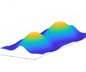
We consider a film of thickness $2 h_\infty$ with a bump localised along the $y$ axis. The reference bump is invariant along the $y$ direction and symmetric with respect to the planes $(0, x,y)$ and $(0, y, z)$. The aim of our work is to establish that an arbitrarily small modulation of the bump height in the $y$ direction (satisfying the two mirror symmetries; see figure 1) is amplified with time, meaning that the invariance under translation of the reference bump is spontaneously broken. Note that the film tends to minimise its interface area and thus relaxes to a flat final state. The question is therefore to determine if its transient shape, during the relaxation process, remains invariant under translation or not.

Figure 1.

Schematic representation of the film and of its non-dimensional dimensions. The reference bump is modulated with a wavelength $\lambda$. A film element is shown in blue, with the expression of the force exerted by the external film on its purple face $(f)$. The black arrows on the left represent the parabolic velocity field, with the interfacial velocity $\boldsymbol {v}$ in red.

The surface tension is $\gamma _0$ at large $|x|$, far from the bump, and slightly varies close to the bump. In order to establish the fact that capillary effects alone are responsible for the spontaneous symmetry breaking, we neglect all other potential destabilising physical processes: disjoining pressure, gravity and inertial effects are not taken into account in our model. For the sake of simplicity, we also neglect the air friction: the damping forces are due to the bulk viscosity $\eta$ and to the interface viscosity $\eta _s$, with the additional assumption that $\eta _s \gg h_\infty \eta$. We assume that the interface Gibbs elasticity is large enough so that the interfaces can be considered as incompressible (Mysels et al. Reference Mysels, Shinoda and Frankel1959), which is the relevant limit for soap films with small (Seiwert, Dollet & Cantat Reference Seiwert, Dollet and Cantat2014; Champougny et al. Reference Champougny, Scheid, Restagno, Vermant and Rio2015) or vanishing (Lenavetier et al. Reference Lenavetier, Audéoud, Berry, Gauthier, Poryles, Trégouët and Cantat2024) external forcing. This condition imposes that

(2.1)\begin{equation} \frac{\partial v_x}{\partial x} + \frac{\partial v_y}{\partial y} = \mbox{div}^{2D}(\boldsymbol{v}) =0 , \end{equation}

with $\boldsymbol {v}(x,y,t)$ the interfacial velocity, assumed to be identical on both interfaces of the film. In this limit the surface tension plays the role of the Lagrange multiplier that prevents the surface from compressing/dilating and the hydrodynamical problem can thus be solved without an additional equation of state for the interface.

The problem is made non-dimensional using $h_\infty$ as the length unit, $\tau = 3 \eta h_\infty /\gamma _0$ as the time unit and $\gamma _0$ as the tension unit. In the following, we use the bar notation for dimensional variables. The equations of motion are determined from the mass and force balances on a film element, defined as the liquid trapped between two pieces of interface ${{\rm d}\kern0.7pt x}\, {{\rm d} y}$, chosen symmetrically in the top and bottom interfaces and followed along their trajectories (see figure 1). The bump width $w$ in the $x$ direction is assumed to be much larger than the film thickness. Under this assumption, the lubrication equations can be used, which are Taylor expansions of the Stokes equations, with the thickness gradient as a small parameter.

2.2. Poiseuille flow

The evolution of the film thickness $2 h(x,y,t)$ is determined from the mass conservation of a film element (Bruinsma Reference Bruinsma1995):

(2.2)\begin{equation} \partial_{t} h + \boldsymbol{v} \boldsymbol{\cdot} \boldsymbol{\nabla} h ={-} \boldsymbol{\nabla} \boldsymbol{\cdot} (h^3 \boldsymbol{\nabla} \Delta h) ,\end{equation}

with $\nabla$ and $\varDelta$ the gradient and Laplacian two-dimensional operators in the $(x,y)$ plane. The left-hand side is the Lagrangian time derivative of the half-thickness of a film element followed along its trajectory. The right-hand side quantifies the flux of liquid leaving the film element due to the relative motion of the liquid with respect to the interfaces (see figure 1). This motion is a Poiseuille flow driven by the Laplace pressure $\Delta h$, with a mean velocity $h^2 \boldsymbol {\nabla } \Delta h$ and a flux $h^3 \boldsymbol {\nabla } \Delta h$. Note that, without this Poiseuille flow, the film element becomes a closed system of constant volume $2 h \,{{\rm d}\kern0.7pt x} \,{{\rm d} y}$. In that case, the thickness is conserved, as the condition ${\rm div}^{2D}(\boldsymbol {v}) =0$ imposes the conservation of the film element area ${{\rm d}\kern0.7pt x}\, {{\rm d} y}$.

2.3. Capillary and viscous stress tensors

The second relationship between $h$ and $\boldsymbol {v}$ is obtained from a force balance on a film element, which also involves the non-dimensional surface tension $\gamma = 1+ \delta \gamma$. An example of a film element of volume $2 h \,{{\rm d}\kern0.7pt x} \,{{\rm d} y}$ is shown in blue in figure 1. The surface tension and pressure forces acting on one of its lateral faces, e.g. its purple face, can be expressed as a function of a two-dimensional stress tensor $\boldsymbol{\mathsf{\sigma}} _{cap}$. This tensor is defined so that the force ${\rm d} \boldsymbol {F}^f$ acting on a face $(f)$ of area $2 h \, {\rm d} \ell ^f$ and of normal $\boldsymbol {n}^f$ is ${\rm d} \boldsymbol {F}^f = \boldsymbol{\mathsf{\sigma}} _{cap} \boldsymbol {\cdot } \boldsymbol {n }^f \, {\rm d} \ell ^f$. In the case of the purple face shown in figure 1, the area is $2 h \,{{\rm d} y}$ and the normal $\boldsymbol {n}^f = \boldsymbol {e}_x$.

This stress depends on the local tension value, on the Laplace pressure $\Delta h$ integrated over the film thickness $2 h$ and on the thickness gradient $\boldsymbol {\nabla } h$. Indeed the interface slope leads to quadratic corrections on the capillary force. The expression of the stress tensor, established in Lenavetier et al. (Reference Lenavetier, Audéoud, Berry, Gauthier, Poryles, Trégouët and Cantat2024), is written below, both in the reference basis $\mathcal {B}_0 = (\boldsymbol {e}_x, \boldsymbol {e}_y)$, with $\boldsymbol {e}_x$ and $\boldsymbol {e}_y$ the unit vectors associated with the directions $x$ and $y$ shown in figure 1, and in a local basis $\mathcal {B}_e = (\boldsymbol {n}, \boldsymbol {t})$ associated with the local film geometry. The unit vector $\boldsymbol {n}$ is oriented in the direction of the thickness gradient, so that $\boldsymbol {\nabla } h= |\boldsymbol {\nabla } h| \boldsymbol {n}$ and $\boldsymbol {t}$ is a unit vector oriented along the lines of constant thickness, $\boldsymbol {t} = \boldsymbol {e}_z \wedge \boldsymbol {n}$. With these conventions, we get

(2.3)\begin{equation} \boldsymbol{\mathsf{\sigma}}_{cap}= \boldsymbol{\mathsf{\sigma}}_{cap}^* + \sigma^f \boldsymbol{\mathsf{I}} , \end{equation}

with $\boldsymbol{\mathsf{I}}$ the identity matrix. The isotropic term

(2.4)\begin{equation} \sigma^f= 2 ( 1 + \delta \gamma) +2 h \Delta h \end{equation}

comes from the Laplace pressure and tension forces. The deviatoric part is

(2.5)\begin{equation} \boldsymbol{\mathsf{\sigma}}_{cap}^* = \begin{pmatrix} - |\boldsymbol{\nabla} h|^2 & 0 \\ 0 & |\boldsymbol{\nabla} h|^2 \end{pmatrix}_{\mathcal{B}_e} ={-} \begin{pmatrix} (\partial_x h)^2 - (\partial_y h)^2 & 2 \partial_x h \partial_y h\\ 2 \partial_x h \partial_y h & (\partial_y h)^2 - (\partial_x h)^2 \end{pmatrix}_{\mathcal{B}_0} .\end{equation}

It arises from the correction of the tension forces, due to their projection in the ($x,y$) plane. A film element is thus submitted to an anisotropic stress, which is higher in the direction perpendicular to the thickness gradient.

The resulting force on the film element is

(2.6)\begin{equation} \boldsymbol{F}_{cap} = \boldsymbol{\nabla} \boldsymbol{\cdot} \boldsymbol{\mathsf{\sigma}}_{cap} = 2 h \boldsymbol{\nabla} (\Delta h) + 2 \boldsymbol{\nabla} \delta \gamma . \end{equation}

For a film of arbitrary thickness, the first term $2 h \boldsymbol {\nabla } (\Delta h)$ is a priori not the gradient of a function and thus cannot be balanced by the second term $2 \boldsymbol {\nabla } \delta \gamma$, whatever the value of the surface tension. The force balance thus requires an additional term, which is here assumed to be the interfacial viscous friction. The viscous stress in a single interface is given by

(2.7)\begin{equation} \boldsymbol{\mathsf{\sigma}}_{vis} = \zeta (\boldsymbol{\nabla} \boldsymbol{v} + (\boldsymbol{\nabla} \boldsymbol{v})^T ) ,\end{equation}

with $\zeta = \eta _s/(\tau \gamma _0) = \eta _s/( 3 \eta h_\infty )$ a dimensionless friction coefficient.

With the interfacial incompressibility condition, the resulting viscous force in a single interface is $\boldsymbol {F}_{vis} = \zeta \Delta \boldsymbol {v}$ and the force balance becomes (Bruinsma Reference Bruinsma1995)

(2.8)\begin{equation} \zeta \Delta \boldsymbol{v} + \boldsymbol{\nabla} \delta \gamma + h \boldsymbol{\nabla} (\Delta h ) =0.\end{equation}

Equations (2.1), (2.2), (2.8) constitute a closed set of equations for the unknown functions $h$, $\delta \gamma$ and $\boldsymbol {v}$ and determine the film evolution from any initial state. This equation set corresponds to the limit of high Marangoni number and low Bond number of the equation set numerically solved in Shi et al. (Reference Shi, Fuller and Shaqfeh2022), with $\zeta$ based on the interfacial viscosity instead of the bulk viscosity.

Our initial condition is shown in figure 1: a flat film with a bump whose height and width are modulated with a wavelength $\lambda$ in the $y$ direction. We restrict our stability analysis to the case $\lambda \gg w$. This assumption allows us to define a near-field domain where $x$ is of the order of $w$ and a far-field domain where $x$ is of the order of $\lambda$. The thickness only varies at the small scale, whereas the velocity is shown to vary at the large scale. We take advantage of this scale separation to simplify further (2.8).

2.4. Line tension

As the thickness gradients are localised in the near-field domain, the line tension formalism is used to express the capillary forces at the large length scale, as proposed in Lenavetier et al. (Reference Lenavetier, Audéoud, Berry, Gauthier, Poryles, Trégouët and Cantat2024). In our geometry, the line tension is defined, for a single interface, as

(2.9)\begin{equation} T = \frac{1}{2}\int_{ -\infty}^\infty \boldsymbol{e}_y \boldsymbol{\cdot} (\boldsymbol{\mathsf{\sigma}}_{cap}- 2 \boldsymbol{\mathsf{I}}) \boldsymbol{\cdot} \boldsymbol{e}_y \,{{\rm d}\kern0.7pt x}.\end{equation}

It represents the force excess in the $\boldsymbol {e}_y$ direction exerted on a line oriented in the $x$ direction, crossing the bump (see figure 2). In the limit where $\partial _x h \gg \partial _y h$, its expression, established in Lenavetier et al. (Reference Lenavetier, Audéoud, Berry, Gauthier, Poryles, Trégouët and Cantat2024), is

(2.10)\begin{equation} T = \int_{ -\infty}^\infty \left(\frac{\partial h}{\partial x} \right)^2 \,{{\rm d}\kern0.7pt x} .\end{equation}

Figure 2.

Scheme of the capillary and viscous forces in the vicinity of the bump. The light-blue domain represents the bump and the grey rectangle the film element of interest. The stress on the red edge, spanning from one side of the bump to the other, is dominated by the capillary stress. Its integral along the edge is, by definition, the line tension. On the black edges, the capillary stress tensor is zero, and the viscous forces dominate.

2.5. Far-field expression of the force balance

We anticipate that the thickness modulation of wavelength $\lambda$ induces a motion in a domain of width $\lambda$ on both sides of the bump. In this far-field domain, the thickness gradients are negligible and (2.8) becomes, for $x \sim \lambda \gg w$,

(2.11)\begin{equation} \zeta \Delta \boldsymbol{v} + \boldsymbol{\nabla} \delta \gamma =0.\end{equation}

The motion is then driven by the boundary conditions at $x \sim w \ll \lambda$. The force balance on the piece of film shown in figure 2, of characteristic size $w\,{{\rm d} y}$, leads to the condition

(2.12)\begin{equation} 2 \frac{\partial T}{\partial y} ={-} 4 \boldsymbol{e}_y \boldsymbol{\cdot} \boldsymbol{\mathsf{\sigma}}_{vis} \boldsymbol{\cdot} \boldsymbol{e}_x (x=w). \end{equation}

As we restrict our stability analysis to degrees of freedom that keep the mirror symmetry $x \to -x$, the $x$ component of the velocity tends to 0 at small scale and we thus have $\partial v_x/\partial y \ll \partial v_y/\partial x$ at $x \sim w$. Using (2.7), the condition (2.12) becomes

(2.13)\begin{equation} \frac{\partial T}{\partial y} ={-} 2 \zeta \frac{\partial v_y}{\partial x} (x=0),\end{equation}

where we used $\partial v_y/\partial x (x=0) = \partial v_y/\partial x (x=w)$ at first order in $w/\lambda$.

To solve the whole stability problem, the far-field velocity field is determined from (2.11) solved for $x>0$, with the boundary condition (2.13). The behaviour of this far-field solution at small $x$ is used to determine the deformation of the thickness pattern due to convection in (2.2).

3.1. Self-similar solution

We first impose that the dynamics of this reference bump remains invariant under translation along the $y$ direction. In this case, the condition of incompressible interfaces ${\rm div}^{2D}\boldsymbol {v}=0$ becomes $\partial v_x/\partial x=0$. Associated with the condition $v_x(0)=0$ given by the symmetry, it imposes the condition of vanishing velocity at the interface. The set of equations of motion is strongly simplified: (2.2) becomes

(3.1)\begin{equation} \partial_{t} h ={-} \partial_x (h^3 \partial_{xxx} h ).\end{equation}

This is a very classical equation which also governs thin films deposited on a solid (Landau & Levich Reference Landau and Levich1942; Hammond Reference Hammond1983; Oron et al. Reference Oron, Davis and Bankoff1997; Chomaz Reference Chomaz2001; Lister et al. Reference Lister, Rallison, King, Cummings and Jensen2006).

Equation (2.8) is no longer useful, but consistently admits a solution with zero velocity for any $y$-invariant thickness field. Indeed it leads to

(3.2)\begin{equation} \delta \gamma ={-} \int_{-\infty}^x h \partial_{xxx} h \, {{\rm d}\kern0.7pt x}',\end{equation}

which provides the tension value if needed.

Equation (3.1) is analytically solved in Benzaquen et al. (Reference Benzaquen, Salez and Raphaël2013) in the linear regime. For a small bump, it becomes

(3.3)\begin{equation} \partial_t h ={-} \partial_{xxxx} h.\end{equation}

The authors show that the profile converges at long time towards an asymptotic self-similar profile:

(3.4)\begin{equation} h^{as}(x,t) =1 + \delta h_0(t) \varPhi\left(\frac{x}{w_0(t)} \right) ,\end{equation}

where $\varPhi$ is the function plotted in figure 3. It is an even function, decreasing exponentially fast at large $x$ and normalised so that $\int _{-\infty }^\infty \varPhi (U) \, {\rm d} U =1$. The functions $\delta h_0$ and $w_0$ are

(3.5a,b)\begin{equation} \delta h_0(t) = A t^{{-}1/4} \quad \mbox{and} \quad w_0(t)= t^{1/4}, \end{equation}

with $A$ the area of the bump section, which is conserved by conservation of the liquid volume. The height of the bump is $\varPhi (0) \delta h_0$ and decreases with time, whereas the bump width $w_0$ increases: the bump spreads on the soap film until it disappears.

Figure 3.

Graph of the function $\varPhi$ given by equation (19) of Benzaquen et al. (Reference Benzaquen, Salez and Raphaël2013) (solid line). The function $-U \varPhi '(U)$ (dashed line) is also used in § 4.

The explicit expression of $\varPhi$ is given in Benzaquen et al. (Reference Benzaquen, Salez and Raphaël2013) and will not be useful in the following. However, we use a few relationships involving this function and its derivative $\varPhi '$, and more generally its derivative $\varPhi ^{(n)}$ of order $n$, which are established below. To shorten the notations, we introduce the auxiliary functions $\varPhi _0(x,t)=\varPhi (x/w_0(t))$ and $\varPhi '_0(x,t)=\varPhi '(x/w_0(t))$.

Using the expressions (3.4) and (3.5a,b), we get the time and space derivatives of $h^{as}$:

(3.6)\begin{gather} \partial_t h^{as}={-} \frac{A}{4} t^{{-}5/4} (\varPhi_0 + x t^{{-}1/4} \varPhi'_0 ) ={-}\frac{1}{4} \frac{\delta h_0}{w_0^4} \left(\varPhi_0 + \frac{x}{w_0} \varPhi'_0 \right) , \end{gather}

(3.7)\begin{gather}\partial_{xxxx} h^{as} = \frac{\delta h_0}{w_0^4} \varPhi^{(4)}_0 . \end{gather}

Using the expressions (3.6) and (3.7) in (3.3), we obtain the differential equation

(3.8)\begin{equation} 4 \varPhi^{(4)}(U) = \varPhi(U) +U \varPhi^{(1)}(U) .\end{equation}

These properties are used below in the following form:

(3.9)\begin{equation} \partial_t (\delta h_0 \varPhi_0 )={-}\frac{\delta h_0}{w_0^4} \varPhi^{(4)}_0 ={-}\frac{\delta h_0}{4 w_0^4} \left( \varPhi_0 + \frac{x}{w_0} \varPhi^{(1)}_0 \right),\end{equation}

directly deduced from (3.3), (3.7) and

(3.10)\begin{equation} \partial_t \left(\frac{\delta h_0}{w_0}\varPhi'_0 \right) = \partial_{t,x} ( \delta h_0 \varPhi_0) ={-}\partial_x \left( \frac{\delta h_0}{w_0^4} \varPhi^{(4)}_0 \right) ={-} \frac{\delta h_0}{ w_0^5} \varPhi^{(5)}_0 .\end{equation}

In this equation, the first and last equalities are obtained by spatial integration and differentiation, respectively, and the second equality is obtained by switching the time and space derivatives and using (3.9).

3.2. Line tension of the reference solution

This bump generates a line tension given by (2.10), the expression for which becomes

(3.11)\begin{equation} T_0 = \int_{ -\infty}^\infty \left(\frac{\delta h_0}{w_0} \varPhi'(U) \right)^2 w_0 \, {\rm d} U = I_1 \frac{\delta h_0^2}{w_0} ,\end{equation}

with

(3.12)\begin{equation} I_1 = \int_{ -\infty}^\infty [\varPhi'(U)]^2 \, {\rm d} U \approx 0.058 .\end{equation}

4.1. Initial perturbation

We assume that, at a given time $t_0$, an arbitrarily small fluctuation of wavelength $\lambda = 2{\rm \pi} /k$ is imposed to the $y$-invariant self-similar profile $h^{as}$ of section area $A$. Note that the choice of the initial time $t_0$ imposes the initial width and height of the reference bump through the relations (3.5a,b). The solution thus depends of the choice of this initial time. For the evolution of the modulated bump, at $t>t_0$, the function is sought in the form

(4.1)\begin{equation} h(x,y,t)= 1 + \delta h(y,t) \varPhi\left(\frac{x}{w(y,t)}\right) ,\end{equation}

with

(4.2a,b)\begin{equation} \delta h=\delta h_0(t) (1+ \varepsilon_h(y,t) ) \quad \mbox{and} \quad w= w_0(t) (1+ \varepsilon_w(y,t) ) ,\end{equation}

as shown in figure 4. This form presumes that, at each $y$ and $t$, the thickness profile keeps its self-similar shape $\varPhi$, which is a strong assumption. The existence of a solution satisfying the form of (4.1) is thus not ensured at this stage, but will be proved a posteriori by exhibiting a solution.

Figure 4.

Scheme of the thickness field given by (4.1). The crest line of the bump is at height $1+\delta h(y,t) \varPhi (0)$, and the characteristic width of the bump is $w(y,t)$.

The functions $\delta h_0(t)$ and $w_0(t)$ are given by (3.5a,b), and the small parameters controlling the fluctuation amplitude are $\varepsilon _h = \hat {\varepsilon }_h(t) \, {\rm e}^{{\rm i}ky}$ for the height and $\varepsilon _w = \hat {\varepsilon }_w(t) \, {\rm e}^{{\rm i}ky}$ for the width of the bump profile.

The functions $\hat {\varepsilon }_h$ and $\hat {\varepsilon }_w$ are assumed to depend on time only. We assume that, for $t>t_0$, $\delta h_0 \ll 1$, $w_0 \ll 1/k$, $\varepsilon _h\ll 1$ and $\varepsilon _w \ll 1$. The equation of motion (2.2) is linearised with respect to $\delta h_0$, $\varepsilon _h$ and $\varepsilon _w$. Equations (2.11) and (2.13) are of quadratic order in $\delta h_0$ and are linearised in $\varepsilon _h$ and $\varepsilon _w$ only.

4.2. Qualitative analysis

Before tackling the full analytical problem, we first qualitatively identify the physical processes involved.

The figure 5 provides a schematic basis to discuss the influence of the height and width perturbations on the time evolution of the bump. The Poiseuille flow, localised at $|x| \sim w$ and represented with blue arrows, is the motion of the fluid with respect to the interfaces. It occurs perpendicularly to the bump and is oriented towards the film. It tends to spread the bump by increasing its width and decreasing its height.

Figure 5.

Schematic top view of the film, with the colour indicating the domain of various thicknesses: the flat film (light blue), the bump (blue) and a positive height fluctuation (darker blue). (a) The local width $w^{loc}$ is larger than the average width $w^{av}$. (b) The local height $h^{loc}$ is larger than the average height $h^{av}$. The amplitude and orientation of the Poiseuille flow, relative to the interfaces, are given by the blue arrows, and the velocity of the interfaces is represented by the red arrows.

Let us first assume that the local width $w^{loc}$ is larger than the average width $w^{av}$, the local bump height $\delta h^{loc}$ remaining at the average height $\delta h^{av}$, as shown in figure 5(a). Locally, the interface curvature and thus the Laplace pressure below the bump are smaller than their average values and the Poiseuille flow ($P$) decreases. As a consequence, the width increases slower than in the rest of the bump ($0< {\rm d} w^{loc}/{\rm d} t|_P < {\rm d} w^{av}/{\rm d} t|_P$) and the height decreases slower (${\rm d} \delta h^{av}/{\rm d} t |_P < {\rm d} \delta h^{loc}/{\rm d} t|_P < 0$). The Poiseuille flow is thus stabilising the width: as $w^{loc}$ grows slower than the width of the remaining part of the bump, the width is uniform again after some time.

However, as the flow no longer needs to remain invariant under translation along the $y$ direction, the interfacial velocity $\boldsymbol {v}$, which was zero in § 3, now plays an important role: the flow is the superposition of $P$ discussed above and a plug flow (i.e. a flow that is uniform through the entire thickness of the film) at a velocity equal to the interfacial velocity $\boldsymbol {v}$. The driving force for this second part of the flow results from the gradients of line tension ($T$). The line tension scales as $\delta h/w^2$ (see (3.11)) and a locally larger width thus induces a smaller line tension. The resulting line-tension gradient along the bump axis $y$ drives a circulation in the film, schematised by the red arrows and circles in figure 5(a): at the point of low line tension, the bump is stretched along its axis $y$ and, by interface incompressibility, it is compressed in the transverse direction $x$. This part of the flow leaves the thickness modulation unchanged (${\rm d}\delta h^{av}/{\rm d} t|_T = {\rm d}\delta h^{loc}/{\rm d} t|_T =0$) but decreases the width (${\rm d} w^{loc}/{\rm d} t|_T < {\rm d} w^{av}/{\rm d} t|_T =0$): this is again a stabilising ingredient for the width.

The total influence of the width fluctuation is obtained by adding the effects of the pressure-induced Poiseuille flow ($P$) and that of the tension-induced recirculation flow ($T$). It can be written in the linear regime as follows:

(4.3a,b)\begin{equation} \frac{{\rm d} (\delta h^{loc}-\delta h^{av})}{{\rm d} t} = a_{hw} (w^{loc} - w^{av}) \quad \mbox{and} \quad \frac{{\rm d} ( w^{loc} - w ^{av})}{{\rm d} t} ={-}a_{ww} (w^{loc} - w^{av}), \end{equation}

with $a_{wh}$ and $a_{ww}$ positive numbers.

The same reasoning can be done with an initial fluctuation of the bump height, as represented in figure 5(b). At a point of larger thickness ($\delta h^{loc} > \delta h^{av}$), the line tension and Laplace pressure are larger, so the opposite scenario occurs: the Poiseuille contribution leads to a faster height decrease ${\rm d} \delta h^{loc}/{\rm d} t |_P < {\rm d} \delta h^{av}/{\rm d} t|_P < 0$ and width increase $0< {\rm d} w^{lav}/{\rm d} t|_P < {\rm d} w^{loc}/{\rm d} t|_P$, whereas the tension contribution does not modify the thickness but imposes $0= {\rm d} w^{av}/{\rm d} t|_T < {\rm d} w^{loc}/{\rm d} t|_T$. The sum of the two contributions leads to

(4.4a,b)\begin{equation} \frac{{\rm d} (\delta h^{loc}-\delta h^{av})}{{\rm d} t} ={-}a_{hh} (\delta h^{loc} - \delta h^{av}) \quad \mbox{and} \quad \frac{{\rm d} ( w^{loc} - w ^{av})}{{\rm d} t} = a_{wh} (\delta h^{loc} - \delta h^{av}), \end{equation}

with $a_{hh}$ and $a_{hw}$ positive numbers.

Finally, considering a single degree of freedom (either the height only or the width only) leads to the conclusion that the invariant solution is stable. However, considering together these two degrees of freedom allows us to built a coupled system which can, in contrast, lead to an instability. Indeed the eigenvalues of the system (4.3a,b), (4.4a,b) satisfy

(4.5)\begin{equation} \omega^2+ \omega( a_{hh}+ a_{ww}) + a_{hh} a_{ww} - a_{hw} a_{wh} =0. \end{equation}

If $a_{hh} a_{ww} < a_{hw} a_{wh}$, one solution is positive and the perturbation grows.

In the following, we determine the coupling coefficients associated with the growth of the unknown functions $\varepsilon _h$ and $\varepsilon _w$ and we show that, indeed, the invariant solution is unstable. The whole destabilisation process can be summarised by the following positive feedback: a positive height fluctuation leads to a higher tension, thus to a local axial compression, thus to a bump width increase, thus to a decrease of the Poiseuille flow, thus to a slowdown of the height decrease and finally to an increase of the initial fluctuation.

4.3. First linearisations

The different equations established in § 2 need to be expanded to first order in $\varepsilon _h$ and $\varepsilon _w$. For any function $F(x/w)$ implicitly written $F$, we define the function $F_0 = F(x/w_0)$. In the following, we use that, at first order in $\varepsilon _w$, we have

(4.6)\begin{equation} F= F_0 - \frac{x}{w_0} \varepsilon_w F'_0 .\end{equation}

4.3.1. Thickness profile derivatives

The thickness profile given by (4.1) is, at first order,

(4.7)\begin{equation} h= 1 + \delta h_0 (1 + \varepsilon_h) \varPhi\left(\frac{x}{w_0(1 + \varepsilon_w )} \right)= 1 + \delta h_0 \varPhi_0 + \varepsilon_h \delta h_0 \varPhi_0 - x \varepsilon_w \frac{\delta h_0}{w_0} \varPhi'_0 , \end{equation}

and its time derivative is

(4.8)\begin{equation} \partial_t h= \partial_t (\delta h_0 \varPhi_0 ) + \varepsilon_h \partial_t (\delta h_0 \varPhi_0 ) - x \varepsilon_w \partial_t \left( \frac{\delta h_0}{w_0} \varPhi'_0\right) + \dot{\varepsilon}_h \delta h_0 \varPhi_0 - x \dot{\varepsilon}_w \frac{ \delta h_0}{w_0} \varPhi'_0 .\end{equation}

4.3.2. Poiseuille flow

We first linearise the Poiseuille term of (2.2), leading to

(4.9)\begin{equation} {-}\boldsymbol{\nabla} \boldsymbol{\cdot} (h^3 \boldsymbol{\nabla} \Delta h ) ={-} \boldsymbol{\nabla} \boldsymbol{\cdot} (\boldsymbol{\nabla} \Delta h ) . \end{equation}

As $1/k \ll w$, the thickness variations are dominated by the $x$ derivative, so

(4.10a,b)\begin{equation} \Delta h = \frac{\delta h}{w^2} \varPhi'' \quad \mbox{and} \quad {-}\boldsymbol{\nabla} \boldsymbol{\cdot} \boldsymbol{\nabla} \Delta h ={-} \frac{\delta h}{w^4} \varPhi^{(4)}.\end{equation}

This latter quantity must now be linearised with respect to $\varepsilon _w$ and $\varepsilon _h$, and using (3.9), (3.10) and (4.6), we get

(4.11)\begin{equation} \left.\begin{array}{c} \displaystyle - \boldsymbol{\nabla} \boldsymbol{\cdot} \boldsymbol{\nabla} \Delta h ={-} \dfrac{\delta h_0}{w_0^4} \varPhi^{(4)} (1+ \varepsilon_h - 4 \varepsilon_w ),\\ \displaystyle - \boldsymbol{\nabla} \boldsymbol{\cdot} \boldsymbol{\nabla} \Delta h={-} \dfrac{\delta h_0}{w_0^4} \varPhi_0^{(4)} (1+ \varepsilon_h - 4 \varepsilon_w ) - x \dfrac{\delta h_0}{w_0^5} \varPhi_0^{(5)} \varepsilon_w ,\\ \displaystyle - \boldsymbol{\nabla} \boldsymbol{\cdot} \boldsymbol{\nabla} \Delta h = \partial_t( \delta h_0 \varPhi_0) (1+ \varepsilon_h - 4 \varepsilon_w ) - x \partial_t\left(\dfrac{\delta h_0}{w_0}\varPhi'_0\right) \varepsilon_w. \end{array}\right\}\end{equation}

4.3.3. Tension

From (2.10), the tension is

(4.12)\begin{equation} T = \int_{ -\infty}^\infty \left(\frac{\delta h}{w} \varPhi'(U) \right)^2 w \, {\rm d} U = \frac{\delta h_0^2}{w_0} (1 + 2 \varepsilon_h - \varepsilon_w ) \int_{ -\infty}^\infty [\varPhi'(U)]^2 \, {\rm d} U , \end{equation}

and using (3.11), we get

(4.13a,b)\begin{equation} T = (1 + 2 \varepsilon_h - \varepsilon_w ) T_0 \quad \mbox{and} \quad \partial_y T= {\rm i} k (2 \varepsilon_h - \varepsilon_w) T_0. \end{equation}

4.4. Far-field recirculation

As discussed in § 2.5, the recirculation flow at the length scale $\lambda$ is governed by (2.11) and the bump properties only appear through the boundary condition (2.13). The velocity field is thus determined in the half-plane $x>0$ from these equations.

As $\textrm {div}^{2D}\boldsymbol {v} = 0$, we introduce the stream function $\phi$ defined as

(4.14a,b)\begin{equation} v_x = \partial_y \phi \quad \mbox{and} \quad v_y ={-} \partial_x \phi, \end{equation}

with $\phi =0$ at large $x$ and

(4.15)\begin{equation} \phi = f(x,t) \, {\rm e}^{{\rm i}ky}.\end{equation}

The two components of (2.11) become

(4.16)\begin{equation} \left.\begin{array}{c} \zeta(\partial_{xx} + \partial_{yy}) \partial_y \phi + \partial_x \delta \gamma = 0, \\ \zeta(\partial_{xx} + \partial_{yy}) \partial_x \phi - \partial_y \delta \gamma = 0. \end{array}\right\} \end{equation}

The unknown tension variation $\delta \gamma$ can be removed by taking the cross-derivatives and combining both equations to obtain

(4.17)\begin{equation} (\partial_{xx} + \partial_{yy}) (\partial_{xx} + \partial_{yy}) \phi =0 . \end{equation}

Using (4.15), we get a fourth-order equation of the function $f$:

(4.18)\begin{equation} f^{(4)} - 2 k^2 f^{(2)} + k^4 f =0 ,\end{equation}

which has $k$ and $-k$ as double roots.

In the domain $x>0$, only the negative value leads to a non-divergent solution (the other half-plane being obtained by symmetry). The condition $v_x(x=0,y)= 0$ imposes $f(x=0, t)=0$, so $f = -\textrm {i} \phi _1 x \, \textrm {e}^{-kx}$, with $\phi _1$ a constant determined below. It leads to

(4.19)\begin{gather} v_x= k \phi_1 x \, {\rm e}^{{-}kx} \, {\rm e}^{{\rm i}ky} , \end{gather}

(4.20)\begin{gather}v_y={-} i \phi_1 (kx -1) \, {\rm e}^{{-}kx} \, {\rm e}^{{\rm i}ky}, \end{gather}

(4.21)\begin{gather}\partial_x v_y={-} i \phi_1 [{-}k (kx -1) +k ] \, {\rm e}^{{-}kx} \, {\rm e}^{{\rm i}ky} , \end{gather}

(4.22)\begin{gather}\partial_x v_y (x=0,y) ={-} 2 {\rm i} k \phi_1 \, {\rm e}^{{\rm i}ky}. \end{gather}

The boundary condition (2.13) imposes, using (4.13b),

(4.23)\begin{equation} \phi_1 = (2 \hat{\varepsilon}_h - \hat{\varepsilon}_w) \frac{T_0}{4 \zeta} .\end{equation}

So, far from the bump, from (4.19), (4.20) and (4.23), we get

(4.24)\begin{gather} v_x= (2 \hat{\varepsilon}_h - \hat{\varepsilon}_w) \frac{T_0}{4 \zeta} k x \, {\rm e}^{{-}kx} \, {\rm e}^{{\rm i}ky} , \end{gather}

(4.25)\begin{gather}v_y={-} {\rm i} (2 \hat{\varepsilon}_h - \hat{\varepsilon}_w) \frac{T_0}{4 \zeta} (kx -1)\, {\rm e}^{{-}kx} \, {\rm e}^{{\rm i}ky}. \end{gather}

This velocity field is shown in figure 6.

Figure 6.

Velocity field $(v_x, v_y)$ given by (4.24), (4.25) as a function of $x/\lambda$ and $y/\lambda$, for $2 \hat {\varepsilon }_h - \hat {\varepsilon }_w> 0$. The bump is schematically represented by the red rectangle.

The convective term involved in (2.2) is $- \boldsymbol {v} \boldsymbol {\cdot } \boldsymbol {\nabla } h$. The term $- v_y \partial _y h$ is of second order in $\varepsilon$ so the convective term becomes $- v_x \partial _x h$, with $\partial _x h = (\delta h_0/w_0) \varPhi '_0$ at the zeroth order in $\varepsilon$. Extrapolating the far-field velocity at the bump, in the small-$x$ domain where ${x \, \textrm {e}^{-kx}\sim x}$, we obtain the convective term involved in the thickness profile evolution:

(4.26)\begin{equation} {-}v_x \partial_x h ={-} x (2 \varepsilon_h - \varepsilon_w) \frac{k T_0}{4 \zeta} \frac{\delta h_0}{w_0} \varPhi'_0 . \end{equation}

4.5. Equation of stability

The Taylor expansion of the equation of motion (2.2) can now be performed using (4.8), (4.11) and (4.26). At the zeroth order in $\varepsilon _h$ and $\varepsilon _w$ we consistently get $\partial _t(\delta h_0 \varPhi _0) = \partial _t(\delta h_0 \varPhi _0)$.

At first order in $\varepsilon$, we get

(4.27)\begin{align} & \varepsilon_h \partial_t (\delta h_0 \varPhi_0 ) - x \varepsilon_w \partial_t \left( \frac{\delta h_0}{w_0} \varPhi'_0\right) + \dot{\varepsilon}_h \delta h_0 \varPhi_0 - x \dot{\varepsilon}_w \frac{ \delta h_0}{w_0} \varPhi'_0 \nonumber\\ &\quad =\partial_t(\delta h_0 \varPhi_0) ( \varepsilon_h - 4 \varepsilon_w ) - x \partial_t\left(\frac{\delta h_0}{w_0}\varPhi'_0\right) \varepsilon_w - x \frac{\delta h_0}{w_0} \varPhi'_0 (2 \varepsilon_h - \varepsilon_w) \frac{k T_0}{4 \zeta} , \end{align}

which is reorganised using (3.9) into

(4.28)\begin{equation} \varPhi_0 \delta h_0 \left( \dot{\varepsilon}_h- \varepsilon_w \frac{1}{w_0^4} \right) + x \varPhi'_0 \frac{ \delta h_0}{w_0} \left( - \dot{\varepsilon}_w - \varepsilon_w \frac{1}{w_0^4} + (2 \varepsilon_h - \varepsilon_w) \frac{k T_0}{4 \zeta} \right) =0 . \end{equation}

We observe only two kinds of $x$-dependencies in the different terms: either functions proportional to $\varPhi _0= \varPhi (x/w_0(t))$ or functions proportional to $x \varPhi '_0=x \varPhi '(x/w_0(t))$. As these two functions are not proportional (see figure 3), the equality (4.28) requires that the prefactor of each one is zero.

We thus get the conditions

(4.29)\begin{equation} \left.\begin{array}{c} \displaystyle \dot{\varepsilon}_h = \varepsilon_w \dfrac{1}{w_0^4}, \\ \displaystyle \dot{\varepsilon}_w ={-} \varepsilon_w \dfrac{1}{w_0^4} + (2 \varepsilon_h - \varepsilon_w) \dfrac{k T_0}{4 \zeta}. \end{array}\right\}\end{equation}

Note that this set of two linear equations no longer involves any dependency in $x$ and admits solutions that are discussed below. This justifies a posteriori the functional choice made for $\delta h$ in (4.1) and (4.2a,b), and the assumption that $\varepsilon _h$ and $\varepsilon _w$ do not depend on $x$.

5.1. Eigenvalues of the system

In the equation set (4.29), the Poiseuille flow and the flow induced by the line tension are governed, respectively, by the characteristic rates $\omega _P= 1/w_0^4$ and $\omega _T = k T_0/(4 \zeta ) = (3 I_1/4) (k \delta h_0^2/w_0) (\eta h_\infty / \eta _s)$. Note that the time scale is $\tau = 3 \eta h_\infty /\gamma _0$, so the associated physical quantities satisfy $\bar {\omega }_P \sim (\delta h_0/w_0)^4 \, \gamma _0/(\eta h_\infty )$ and $\bar {\omega }_T \sim \delta h_0^2/(\lambda w_0) \, \gamma _0/\eta _s$. As anticipated in § 4.2, the driving force is always the minimisation of the interface energy, proportional to $\gamma _0$. Moreover, the damping force is either the bulk friction proportional to $\eta$, due to a motion of the liquid phase with respect to the interfaces, or the interface friction proportional to $\eta _s$, due to in-plane recirculations in the film.

With these notations, the system (4.29) becomes

(5.1)\begin{equation} \frac{{\rm d} }{{\rm d} t} \begin{bmatrix} \varepsilon_h \\ \varepsilon_w \end{bmatrix} = \begin{bmatrix} 0 & \omega_P\\ 2 \omega_T & - \omega_T - \omega_P \end{bmatrix} \begin{bmatrix} \varepsilon_h \\ \varepsilon_w \end{bmatrix} .\end{equation}

Coming back to our qualitative analysis in § 4.2, we get the expected signs in the matrix. Note, however, that one coupling coefficient is zero. This comes from the fact that we work here with the relative height perturbation $\varepsilon _h$ and not with the local bump height $\delta h_0 (1 +\varepsilon _h)$ as previously. The Poiseuille flow is proportional to the bump height (see (4.11)), leading to the cancellation of the two terms proportional to $\varepsilon _h$ in (4.27).

The eigenvalues of (5.1) are

(5.2)\begin{equation} \omega^\pm = \tfrac{1}{2} (-(\omega_T+ \omega_P) \pm \sqrt{(\omega_T+\omega_P)^2 + 8 \omega_T \omega_P}) ,\end{equation}

and the associated eigenvectors $(\varepsilon _h, \varepsilon _w)^\pm =(1, \omega ^\pm /\omega _P)$. The growth rate $\omega ^+$ is strictly positive if both $\omega _T$ and $\omega _P$ are strictly positive, so the corresponding initial fluctuation can a priori grow.

The asymptotic behaviour of $\omega ^+$ is $2 \omega _P$ at large $\omega _T/\omega _P$ and $2 \omega _T$ at small $\omega _T/\omega _P$, as shown in figure 7. The growth rate is thus dominated by the slowest process, either the Poiseuille flow, driven by $\omega _P$, or the tension-induced recirculation, driven by $\omega _T$. As expected from § 4.2, the instability disappears if one of the two processes becomes infinitely slow, i.e. if the corresponding characteristic rate ($\omega _P$ or $\omega _T$) vanishes. If both processes evolve on the same time scale, $\omega _T=\omega _P = \omega _{T,P}$ and the growth rate becomes $\omega ^+ = (\sqrt {3}-1) \omega _{T,P} \approx 0.73 \omega _{T,P}$.

Figure 7.

Growth rate $\omega ^+$ of the instability as a function of $\omega _T$ and $\omega _P$, as given by (5.2). Some level curves are shown in black, for integer values of $\omega ^+$.

The negative eigenvalue $\omega ^-$ scales as $-\omega _P$ and as $-\omega _T$, respectively, at small and large $\omega _T/\omega _P$ and is thus dominated by the fastest process.

5.2. System solution

5.2.1. Explicit time-dependent equations

Using expression (3.5a,b) for the reference bump and expression (3.11) for the line tension, (4.29) becomes

(5.3)\begin{gather} \dot{\varepsilon}_h = t^{{-}1} \varepsilon_w , \end{gather}

(5.4)\begin{gather}\dot{\varepsilon}_w ={-} t^{{-}1} \varepsilon_w + t^{{-}3/4} K (2 \varepsilon_h - \varepsilon_w), \end{gather}

with $K= k I_1 A^2/(4 \zeta )$, $I_1$ a number defined in (3.11) and $A$ the invariant bump area, as defined in (3.5a,b).

To simplify the time dependency, we define a new time variable $\varTheta = 4 K t^{1/4}$ so $t= ( \varTheta /(4K) )^4$, and the associated unknown functions $X(\varTheta ) = \hat {\varepsilon }_h(t)$ and $Y(\varTheta ) = \hat {\varepsilon }_w(t)$ for the height and the width.

After the change of variable, (5.3) and (5.4) become

(5.5)\begin{equation} \frac{{\rm d} }{{\rm d} \varTheta} \begin{bmatrix} X \\ Y \end{bmatrix} = \begin{bmatrix} 0 & \varOmega_P\\ 2 \varOmega_T & - \varOmega_T - \varOmega_P \end{bmatrix} \begin{bmatrix} X \\ Y \end{bmatrix} \quad \mbox{with} \quad \varOmega_P=\frac{4}{\varTheta} \quad \mbox{and} \quad \varOmega_T=1 .\end{equation}

This system is formally identical to (5.1) and its two eigenvalues $\varOmega ^+$ and $\varOmega ^-$ are thus deduced from (5.2). At large $\varTheta$, $\varOmega ^+$ scales as $2 \varOmega _P= 8/\varTheta$ and $\varOmega ^-$ tends to $-\varOmega _T= -1$.

5.2.2. A polynomial solution

As the positive eigenvalue tends to $0$ at large $\varTheta$, we guess the existence of a growing solution $(X^+,Y^+)$ with a power-law behaviour and we try to build a solution of the form

(5.6a,b)\begin{equation} X^+=\varTheta^N {\sum_{j=0}^{\infty}} a_j \varTheta^{{-}j} \quad \mbox{and} \quad Y^+=\varTheta^N {\sum_{j=0}^{\infty}} b_j \varTheta^{{-}j}, \end{equation}

satisfying, from (5.5),

(5.7a,b)\begin{equation} \frac{{\rm d} X^+}{{\rm d} \varTheta}= \frac{4}{\varTheta} Y^+ \quad \mbox{and} \quad \frac{{\rm d} Y^+}{{\rm d} \varTheta}= 2 X^+- \left( \frac{4}{\varTheta} + 1\right) Y^+ . \end{equation}

These conditions lead, for the terms of highest order ($\,j=0$), to

(5.8a,b)\begin{equation} N a_0 = 4 b_0 \quad \mbox{and} \quad 2 a_0 -b_0 = 0 ,\end{equation}

which imposes $N=8$.

For the generic terms $j \ge 0$, we thus get the conditions

(5.9a,b)\begin{equation} (8-j) a_j = 4 b_j \quad \mbox{and} \quad 2a_{j+1} - b_{j+1} = b_j (12-j), \end{equation}

and after substitution of the first relation in the second, we get

(5.10)\begin{equation} a_{j+1} = a_j \frac{(8-j)(12-j)}{1+j} .\end{equation}

The coefficients $a_j$ are zero for $j>8$ and a solution of (5.5) is the polynomial

(5.11a,b)\begin{equation} X^+={\sum_{j=0}^{8}} a_j \varTheta^{8-j}; \quad Y^+= {\sum_{j=0}^{7}} a_j \frac{8-j}{4} \varTheta^{8-j},\end{equation}

with $a_0=1$ arbitrarily chosen and, from (5.10),

(5.12a,b)\begin{equation} a_j= \frac{8! 12!}{(8-j)!(12-j)!j!} \quad \mbox{and} \quad b_j= \frac{(8-j) 8! 12!}{4(8-j)!(12-j)!j!} . \end{equation}

This explicit solution of the problem diverges at large time and thus provides evidence that the invariant bump is unstable.

Another solution $(X^-,Y^-)$, decreasing faster than exponentially, can also be built (see (A9) in Appendix A). All the solutions can be written as $(X,Y)=a^+ (X^+,Y^+) + a^- (X^-, Y^-)$ with $a^+$ and $a^-$ two prefactors determined from the initial conditions at $\varTheta _0= 4 K t_0^{1/4}$, with $t_0$ the arbitrary initial time defined in § 4.1.

For the purpose of illustration, and to check our computations, the numerical integration of (5.5) has been performed with Matlab. The trajectories obtained for a set of initial conditions satisfying $X^2+ Y^2= 0.01$ at the arbitrary time $\varTheta _0=1$ are plotted in figure 8. It shows a divergence at large time, except for a particular initial condition, corresponding to the stable solution. The functions $X(\varTheta )$ and $Y(\varTheta )$ are shown in figure 9 as a function of time, for the same initial conditions as in figure 8. They have been divided by $X(6)$ to provide evidence that the large-$\varTheta$ behaviour does not depend on the initial condition. Indeed, at large time, all the solutions are proportional to the polynomial solution $(X^+,Y^+)$ as expected.

Figure 8.

Numerical trajectories in the $(X,Y)$ plane, with an initial condition $(X_0,Y_0)= 0.1 (\cos (\theta ),\sin (\theta ))$ at $\varTheta =1$, obtained by solving (5.5). All trajectories diverge at long time, except that obtained with $\theta \approx 2.12 [{\rm \pi} ]$ rad, corresponding to the stable solution (dashed lines). The arrows indicate the direction of the trajectories and the time $\varTheta =2.5$ (arbitrarily chosen but visible on most of the trajectories) is indicated by a circle of the same colour as the curve. Note that the yellow circles are hidden by the blue ones, and green ones are not shown as they would be outside the figure.

Figure 9.

Numerical values of $X(\varTheta )/X(6)$ (a) and $Y(\varTheta )/X(6)$ (b), obtained by solving (5.5). The colour code is the same as in figure 8 and thus indicates the initial condition. The red circles represent the analytical solutions $(X^+/X^+(6),Y^+/X^+(6))$, given by (5.11a,b).

5.3. Physical growth rate of the instability

In the following we consider only the contribution of the unstable mode (denoted with ‘$+$’), for $t> t_0$, and we come back to the physical variables, using the bar notation when needed. The explicit expression of the relative amplitude fluctuation of the unstable mode is directly deduced from the solution (5.11a,b), (5.12a,b), using the definition of the function $(X,Y)$ given in § 5.2.1:

(5.13)\begin{gather} \hat{\varepsilon}^+_h=\alpha {\sum_{j=0}^{8}} \frac{8! 12!}{(8-j)!(12-j)!j!} \left(\frac{\bar{t}}{\tau (4 K)^{{-}4}}\right)^{({8-j})/{4}} , \end{gather}

(5.14)\begin{gather}\hat{\varepsilon}^+_w=\alpha {\sum_{j=0}^{7}} \frac{8! 12!}{(8-j)!(12-j)!j!} \frac{8-j}{4} \left(\frac{\bar{t}}{\tau (4 K)^{{-}4}}\right)^{({8-j})/{4}}, \end{gather}

with $K= k I_1 A^2/(4 \zeta )$ a parameter proportional to the wavenumber $k$ and $\alpha$ a prefactor determined by the initial amplitude fluctuation, small enough to ensure that $\hat {\varepsilon }^+_{h,w} \ll 1$. Note that, as we consider the unstable mode only, the initial values of $\hat {\varepsilon }^+_h$ and $\hat {\varepsilon }^+_w$ are not independent.

At large time, the solution behaves as

(5.15a,b)\begin{equation} \hat{\varepsilon}^+_h \sim \alpha \left(\frac{\bar{t}}{\tau (4 K)^{{-}4}}\right)^2 , \quad \hat{\varepsilon}^+_w \sim 2 \alpha \left(\frac{\bar{t}}{\tau (4 K)^{{-}4}}\right)^2.\end{equation}

In order to get some orders of magnitude, we set the physical parameters to the values presented in table 1 (left). The chosen tension and viscosity correspond to usual surfactant solutions. In order to keep the viscous parameter $\zeta = \eta _s/(3 \eta h_\infty )$ close to unity, we choose to consider an interface shear viscosity of $10^{-8}\ \textrm {kg}\ \textrm {s}^{-1}$, which should be reached for highly soluble surfactants (Zell et al. Reference Zell, Nowbahar, Mansard, Leal, Deshmukh, Mecca, Tucker and Squires2014). Note that the friction of air may play a role for such a low interface viscosity, which has not been considered in the model (Lenavetier et al. Reference Lenavetier, Audéoud, Berry, Gauthier, Poryles, Trégouët and Cantat2024). With these values, the time scale and the viscous parameter are calculated and presented in table 1 (left). As initial bump shape, we choose the self-similar shape of height $\bar {h}^b(\bar {t}_0)= h_\infty \varPhi (0) \delta h_0(t_0) = 200$ nm and of width $\bar {w}(\bar {t}_0)=h_\infty w_0(t_0)= 30\ \mathrm {\mu }$m. As the aspect ratio of the bump evolves with time following (3.5a,b), these choices impose the value of the initial time $t_0$ and of the geometrical parameter $A$, which are specified in table 1 (centre). Finally, the initial height perturbation is $1\,\%$ of $\delta \bar {h}_0$.

Table 1.

Parameters used for the numerical application. Left column: soap film and subsequent parameters. Centre column: initial bump at the onset of instability ($t=t_0$). Right column: initial perturbation. The top parts of the table are the chosen physical parameters and the bottom parts are the corresponding numerical parameters.

The value of $\hat {\varepsilon }^+_h$ is plotted in figure 10(a) for the wavelengths $\bar {\lambda }=[1, 2, 5, 10] \bar {w}_0$, for the time range satisfying the constraint $\hat {\varepsilon }^+_h < 0.3$. Note that only the last case satisfies the condition $\lambda \gg w_0$ assumed in the model, and that the other cases should be considered as extrapolated results. However, as the short-wavelength cases are the most unstable modes, the physical destabilisation process is expected to be close to these extrapolated modes. The contribution of each term of the polynomial (5.13) is plotted in figure 10(b). Low-order monomials dominate at short time, while high-order monomials only make a significant contribution at long time. For the example shown in figure 10, at the end of the linear regime at $\bar {t} - \bar {t}_0 \sim 0.5$ s, the largest contribution comes from the $\bar {t}^{7/8}$ term so the power law (5.15a,b) is never observed.

Figure 10.

(a) Fluctuation amplitude divided by the bump height $\hat {\varepsilon }_h(\bar {t})$, predicted by (5.13), for the physical parameters given in table 1. The wavelength is $\lambda =[1, 2, 5, 10] w_0$, respectively, for the magenta, red, green and blue curves. (b) Value of the different monomials in (5.13) for $\lambda = 2 w_0$, from the $\bar {t}^{3/8}$ term (yellow) to the $\bar {t}^2$ term (dark brown). The monomials of lower orders are indistinguishable from zero. The dominant terms are the monomial $\bar {t}^{3/2}$ and $\bar {t}^{7/4}$, respectively, before and after $\bar {t} = 0.57$ s. The asymptotic power law, dominated by the $\bar {t}^2$ term, would only be reached after $\bar {t} = 22$ s.

In order to characterise more precisely the bump shape, we define its maximal height $\bar {h}^{max}(\bar {t}) = h_\infty \varPhi (0) \delta h_0(\bar {t}) (1+ \hat {\varepsilon }^+_h)$, reached at the point $(\bar {x}=0, \bar {y}=0)$, and the height at the saddle points along the bump crest $\bar {h}^{sad}(\bar {t}) = h_\infty \varPhi (0) \delta h_0(\bar {t}) (1- \hat {\varepsilon }^+_h)$, reached at the point $(\bar {x}=0, \bar {y}=\bar {\lambda }/2)$. These characteristic heights are plotted in figure 11 as a function of time, for the same parameter and wavelength values as in figure 10. In this representation, the fate of the initially invariant bump clearly appears. The saddle-point height decreases faster than the average bump height, and the height of the maximum also decreases with time, but slower than the average bump height. Note that the thickness is only modified by the Poiseuille flow, which leads to a thickness decrease at every point along the bump crest: the increase of $\bar {h}^{max}$ observed at long time for the shortest wavelength is thus unphysical and comes from the fact that the system has left the linear regime. The difference between the maximum height and the saddle-point height $\bar {\delta h}^* = (\bar {h}^{max} - \bar {h}^{sad})/2 = h_\infty \varPhi (0) \delta h_0 \hat {\varepsilon }^+_h$ quantifies the absolute amplitude of the perturbation. As $\delta h_0 \sim \bar {t}^{-1/4}$ and $\hat {\varepsilon }^+_h$ grows with an apparent power law in the range $\bar {t}^{[1.5- 2]}$, the perturbation amplitude grows slightly faster than linearly.

Figure 11.

Geometrical properties of the bump as a function of time in physical units. The wavelength is $\lambda =[1, 2, 5, 10] w_0$, respectively, for the magenta, red, green and blue curves. (a) The top curves are the maximal height $\bar {h}^{max}$ and the bottom curves the saddle-point height $\bar {h}^{sad}$. The black dashed line is the average bump height. (b) Similarly, the top and bottom curves are the maximal and minimal values of the bump width $\bar {w}$ and the black dashed line is the average bump width.

The minimum and maximum widths of the perturbation are shown in figure 11. Importantly $\hat {\varepsilon }^+_h$ and $\hat {\varepsilon }^+_w$ have the same sign, so the width increases at the places of maximum height. A three-dimensional profile built from (5.13), (5.14) with parameters of table 1 is shown in figure 12(a,b) and shows this transition from the initial invariant bump towards well-separated round hills expected at long time (Trégouët & Cantat Reference Trégouët and Cantat2021). The shape evolution is also plotted for a groove in figure 12(c,d) to underline that the whole study remains valid for a negative value of $\delta h_0$, so a groove instead of a bump, as potentially relevant for the marginal regeneration problem.

Figure 12.

Examples of film-thickness profiles calculated with the parameters of table 1 (a,b) or with the same parameters but for a groove of initial depth $\bar {h}^b(\bar {t}_0) = - 0.2 h_\infty$ (c,d). The initial perturbations are shown in (a,c) and the profiles after 500 ms are shown in (b,d), for $\lambda = 20 \bar {w}(\bar {t}_{0})$. The colour bar represents $|\bar {h} - h_\infty |$ in micrometres.

Another important point is that the growth is faster at small wavelength. The model assumes $\lambda \gg w_0$, so the small-wavelength limit cannot be discussed in this frame. As a consequence, this model does not predict the fastest wavelength. A reasonable guess is that this fastest wavelength is of the order of the bump width.