


1 Introduction
Let
 $T=T_{\pi ,\unicode{x3bb} }:[0,1)\to [0,1)$
be an interval exchange transformation (IET) given by an irreducible permutation
$T=T_{\pi ,\unicode{x3bb} }:[0,1)\to [0,1)$
be an interval exchange transformation (IET) given by an irreducible permutation
 $\pi =(\pi _0,\pi _1)$
(where
$\pi =(\pi _0,\pi _1)$
(where
 $\pi _0,\pi _1:\mathcal {A}\to \{1,\ldots ,d\}$
are bijections describing the position of intervals, labeled by elements of
$\pi _0,\pi _1:\mathcal {A}\to \{1,\ldots ,d\}$
are bijections describing the position of intervals, labeled by elements of
 $\mathcal {A}$
, before and after the translation) and by the vector
$\mathcal {A}$
, before and after the translation) and by the vector
 $\unicode{x3bb} =(\unicode{x3bb} _\alpha )_{\alpha \in \mathcal {A}}$
collecting the lengths of exchanged intervals. Denote by
$\unicode{x3bb} =(\unicode{x3bb} _\alpha )_{\alpha \in \mathcal {A}}$
collecting the lengths of exchanged intervals. Denote by
 $I_\alpha =[l_\alpha ,r_\alpha )$
,
$I_\alpha =[l_\alpha ,r_\alpha )$
,
 $\alpha \in \mathcal {A}$
, the intervals exchanged by T. We mainly deal with symmetric IETs, that is,
$\alpha \in \mathcal {A}$
, the intervals exchanged by T. We mainly deal with symmetric IETs, that is,
 $\pi _0(\alpha )+\pi _1(\alpha )=d+1$
for any
$\pi _0(\alpha )+\pi _1(\alpha )=d+1$
for any
 $\alpha \in \mathcal {A}$
. If
$\alpha \in \mathcal {A}$
. If
 $\mathcal {I}:[0,1]\to [0,1]$
is the reflection across
$\mathcal {I}:[0,1]\to [0,1]$
is the reflection across
 $1/2$
, that is,
$1/2$
, that is,
 $\mathcal {I} x=1-x$
, then
$\mathcal {I} x=1-x$
, then
 $\mathcal {I}\circ T=T^{-1}\circ \mathcal {I}$
and this map acts on every interval
$\mathcal {I}\circ T=T^{-1}\circ \mathcal {I}$
and this map acts on every interval
 $I_\alpha $
as the reflection across the center of
$I_\alpha $
as the reflection across the center of
 $I_\alpha $
denoted by
$I_\alpha $
denoted by
 $m_\alpha $
.
$m_\alpha $
.
The main objective of this paper is to develop novel methods to prove the ergodicity of skew products
 $T_f:[0,1)\times \mathbb {R}\to [0,1)\times \mathbb {R}$
of the form
$T_f:[0,1)\times \mathbb {R}\to [0,1)\times \mathbb {R}$
of the form
 $T_f(x,r)=(Tx,r+f(x))$
, where
$T_f(x,r)=(Tx,r+f(x))$
, where
 $f:[0,1)\to \mathbb {R}$
is a
$f:[0,1)\to \mathbb {R}$
is a
 $C^1$
-map on the interior of all exchanged intervals and having singularities at their ends. Suppose that
$C^1$
-map on the interior of all exchanged intervals and having singularities at their ends. Suppose that
 $$ \begin{align} \theta\ {:}\ &[x_0,+\infty)\to\mathbb{R}_{>0} \text{ is an increasing } C^1\text{-map such that } \int_{x_0}^{+\infty}\frac{dx}{x\theta(x)}=+\infty, \nonumber\\ & \text{ and the map } \tau:(0,x_0^{-1}]\to\mathbb{R}_{>0} \text{ given by } \tau(s)=\frac{s^2}{\theta'(1/s)} \text{ is increasing.}\quad \end{align} $$
Notice that we can always extend the functions
 $\theta $
and
$\theta $
and
 $\tau $
so that
$\tau $
so that
 $x_0 = 1$
while preserving the properties above.
$x_0 = 1$
while preserving the properties above.
In this work, we consider maps with singularities that behave like
 $s\mapsto \theta (1/s)$
. More precisely, we deal with the space
$s\mapsto \theta (1/s)$
. More precisely, we deal with the space
 $\Upsilon _\theta (\bigsqcup _{\alpha \in \mathcal {A}} I_{\alpha })$
of functions
$\Upsilon _\theta (\bigsqcup _{\alpha \in \mathcal {A}} I_{\alpha })$
of functions
 $f:[0,1)\to \mathbb {R}$
which are
$f:[0,1)\to \mathbb {R}$
which are
 $C^1$
on the interior of all exchanged intervals
$C^1$
on the interior of all exchanged intervals
 $I_{\alpha }$
,
$I_{\alpha }$
,
 $\alpha \in \mathcal {A}$
and
$\alpha \in \mathcal {A}$
and
 $$ \begin{align} Z_\theta(f):=\max_{\alpha\in\mathcal{A}}\Big\{\!\sup_{x\in(l_\alpha,m_\alpha]}| f'(x)\tau(x-l_\alpha)|,\sup_{x\in[m_\alpha,r_\alpha)}|f'(x)\tau(r_\alpha-x)|\Big\}<+\infty. \end{align} $$
For any
 $f\in \Upsilon _\theta (\bigsqcup _{\alpha \in \mathcal {A}} I_{\alpha })$
let
$f\in \Upsilon _\theta (\bigsqcup _{\alpha \in \mathcal {A}} I_{\alpha })$
let
 $$ \begin{align} z_\theta(f):=\max_{\alpha\in\mathcal{A}}\Big\{\!\inf_{x\in(l_{\alpha},m_{\alpha}]}|f'(x) \tau(x-l_{\alpha})|, \inf_{x\in[m_{\alpha},r_{\alpha})}|f'(x)\tau(r_{\alpha}-x)|\Big\}. \end{align} $$
Roughly speaking, the positivity of
 $z_\theta (f)$
expresses non-triviality of at least one singularity of the type
$z_\theta (f)$
expresses non-triviality of at least one singularity of the type
 $s\mapsto \theta (1/s)$
.
$s\mapsto \theta (1/s)$
.
In this paper, we focus on the ergodic properties of skew products
 $T_f$
when the function f is additionally anti-symmetric, which means that
$T_f$
when the function f is additionally anti-symmetric, which means that
 $f\circ T^{-1}\circ \mathcal {I}=-f$
, so is anti-symmetric with respect to the central reflection of any interval
$f\circ T^{-1}\circ \mathcal {I}=-f$
, so is anti-symmetric with respect to the central reflection of any interval
 $I_\alpha $
,
$I_\alpha $
,
 $\alpha \in \mathcal {A}$
. Moreover, we say that f is piecewise monotonic if f is increasing when restricted to the interior of each interval
$\alpha \in \mathcal {A}$
. Moreover, we say that f is piecewise monotonic if f is increasing when restricted to the interior of each interval
 $I_\alpha $
,
$I_\alpha $
,
 $\alpha \in \mathcal {A}$
, or is always decreasing.
$\alpha \in \mathcal {A}$
, or is always decreasing.
The main basic result of the paper, based on ideas developed in [Reference Fayad and Lemańczyk6] for rotations, is the following theorem.
Theorem 1.1. Let
 $\theta :[x_0,+\infty )\to \mathbb {R}_{>0}$
, with
$\theta :[x_0,+\infty )\to \mathbb {R}_{>0}$
, with
 $x_0>0$
, be a slowly varying, increasing
$x_0>0$
, be a slowly varying, increasing
 $C^1$
-map such that
$C^1$
-map such that
 $\int _{x_0}^{+\infty }({dx}/{x\theta (x)})=+\infty $
and the map
$\int _{x_0}^{+\infty }({dx}/{x\theta (x)})=+\infty $
and the map
 $x\mapsto x^2\theta '(x)$
is increasing. Then, for almost every (a.e.) symmetric IET T, if
$x\mapsto x^2\theta '(x)$
is increasing. Then, for almost every (a.e.) symmetric IET T, if
-
(1)
 $f\in \Upsilon _\theta (\bigsqcup _{\alpha \in \mathcal {A}}I_{\alpha })$
with
$z_\theta (f)>0$
,
$f\in \Upsilon _\theta (\bigsqcup _{\alpha \in \mathcal {A}}I_{\alpha })$
with
$z_\theta (f)>0$
, -
(2) f is anti-symmetric,
-
(3) f is piecewise monotonic,

then the skew product
 $T_f$
is ergodic.
$T_f$
is ergodic.
This theorem and its generalisation in the form of Theorem 6.3 are directly applicable to the study of the behavior of error terms in the spectral decomposition of Birkhoff integrals for locally Hamiltonian flows on compact surfaces when all saddles are perfect. The aforementioned spectral decomposition has recently been studied in [Reference Frączek and Ulcigrai12] (for non-degenerate saddles) and in [Reference Frączek and Kim8] (more generally, when all saddles are perfect). We present all the details in §2. One of the main results of [Reference Frączek and Ulcigrai12] is the proof of the equidistribution of the error term when almost every flow has no saddle loops, which is a consequence of the ergodicity of a certain skew extension of the flow. In turn, the ergodicity of the extension follows from the ergodicity of a certain skew product
 $T_f$
for f having logarithmic singularities of symmetric type.
$T_f$
for f having logarithmic singularities of symmetric type.
One of the goals of the present paper is to show that the error term is equidistributed also when the locally Hamiltonian flow has saddle loops. In this case, the methods developed so far (mainly based on techniques derived from [Reference Conze and Frączek5]) fail because the symmetry condition is broken. To overcome this problem, we use a version of Theorem 1.1 for
 $\theta =\log $
to prove the equidistribution of the error term in the case of locally Hamiltonian flows (with perfect saddles) of hyperelliptic type (see Theorem 2.4), which constitutes another main result of the paper.
$\theta =\log $
to prove the equidistribution of the error term in the case of locally Hamiltonian flows (with perfect saddles) of hyperelliptic type (see Theorem 2.4), which constitutes another main result of the paper.
However, Theorem 1.1 also has applications beyond the use of the logarithmic function. In Appendix A, we construct a family of locally Hamiltonian flows with a new type of degenerate and imperfect saddles whose anti-symmetric skew product extensions are ergodic. This is an entirely new class of ergodic skew products unknown even in the context of extensions of rotations.
2 Applications to locally Hamiltonian flows on compact surfaces
Let M be a smooth, compact, connected, orientable surface of genus
 $g\geq 1$
. We focus on smooth flows
$g\geq 1$
. We focus on smooth flows
 $\psi _{\mathbb {R}} = (\psi _t)_{t\in \mathbb {R}}$
on M preserving a smooth area form
$\psi _{\mathbb {R}} = (\psi _t)_{t\in \mathbb {R}}$
on M preserving a smooth area form
 $\omega $
, that is, such that for any (orientable) local coordinates
$\omega $
, that is, such that for any (orientable) local coordinates
 $(x,y)$
, we have
$(x,y)$
, we have
 $\omega =V(x,y)\,dx\wedge dy$
with V positive and smooth. Then, for (orientable) local coordinates
$\omega =V(x,y)\,dx\wedge dy$
with V positive and smooth. Then, for (orientable) local coordinates
 $(x,y)$
such that
$(x,y)$
such that
 $\omega =V(x,y)\,dx\wedge dy$
, the flow
$\omega =V(x,y)\,dx\wedge dy$
, the flow
 $\psi _{\mathbb {R}}$
is (locally) a solution to the Hamiltonian equation
$\psi _{\mathbb {R}}$
is (locally) a solution to the Hamiltonian equation
 $$ \begin{align*} \frac{dx}{dt} = \frac{({\partial H}/{\partial y})(x,y)}{V(x,y)},\quad \frac{dy}{dt} = -\frac{({\partial H}/{\partial x})(x,y)}{V(x,y)}, \end{align*} $$
for a smooth real-valued locally defined function H, or equivalently
 ${dz}/{dt}=-2\iota {({\partial H}/{\partial \overline {z}})(z,\overline {z})}/{V(z,\overline {z})}$
in complex variables. The flows
${dz}/{dt}=-2\iota {({\partial H}/{\partial \overline {z}})(z,\overline {z})}/{V(z,\overline {z})}$
in complex variables. The flows
 $\psi _{\mathbb {R}}$
are usually called locally Hamiltonian flows or multivalued Hamiltonian flows.
$\psi _{\mathbb {R}}$
are usually called locally Hamiltonian flows or multivalued Hamiltonian flows.
For any smooth observable
 $f: M\to \mathbb {R}$
, we are interested in understanding the asymptotic behavior of the so-called Birkhoff integrals
$f: M\to \mathbb {R}$
, we are interested in understanding the asymptotic behavior of the so-called Birkhoff integrals
 $$ \begin{align*} \int_0^Tf(\psi_tx)\,dt\quad\text{as } T\to+\infty. \end{align*} $$
We always assume that all fixed points of the flow
 $\psi _{\mathbb {R}}$
are isolated, so the set
$\psi _{\mathbb {R}}$
are isolated, so the set
 $\mathrm {Fix}(\psi _{\mathbb {R}})$
of fixed points of
$\mathrm {Fix}(\psi _{\mathbb {R}})$
of fixed points of
 $\psi _{\mathbb {R}}$
is finite and, if
$\psi _{\mathbb {R}}$
is finite and, if
 $g \geq 2$
, then it is non-empty. As
$g \geq 2$
, then it is non-empty. As
 $\psi _{\mathbb {R}}$
is area-preserving, fixed points are either centers, simple saddles, or multi-saddles (saddles with
$\psi _{\mathbb {R}}$
is area-preserving, fixed points are either centers, simple saddles, or multi-saddles (saddles with
 $2k$
prongs with
$2k$
prongs with
 $k \geq 2$
). In this paper, we will mainly consider perfect (also known as harmonic) saddles. A fixed point
$k \geq 2$
). In this paper, we will mainly consider perfect (also known as harmonic) saddles. A fixed point
 $\sigma \in \mathrm {Fix}(\psi _{\mathbb {R}})$
is a (perfect) saddle of multiplicity
$\sigma \in \mathrm {Fix}(\psi _{\mathbb {R}})$
is a (perfect) saddle of multiplicity
 $m=m_\sigma \geq 2$
if there exists a chart
$m=m_\sigma \geq 2$
if there exists a chart
 $(x,y)$
(called a singular chart) in a neighborhood
$(x,y)$
(called a singular chart) in a neighborhood
 $U_\sigma $
of
$U_\sigma $
of
 $\sigma $
such that
$\sigma $
such that
 $\omega =V(x,y)\,dx\wedge dy$
and
$\omega =V(x,y)\,dx\wedge dy$
and
 $H(x,y)=\Im (x+\iota y)^m$
(
$H(x,y)=\Im (x+\iota y)^m$
(
 $(0,0)$
are coordinates of
$(0,0)$
are coordinates of
 $\sigma $
). Then the corresponding local Hamiltonian equation in
$\sigma $
). Then the corresponding local Hamiltonian equation in
 $U_\sigma $
is of the form
$U_\sigma $
is of the form
 ${dz}/{dt}={m\overline {z}^{m-1}}/{V(z,\overline {z})}$
. We denote the set of perfect saddles of
${dz}/{dt}={m\overline {z}^{m-1}}/{V(z,\overline {z})}$
. We denote the set of perfect saddles of
 $\psi _{\mathbb {R}}$
by
$\psi _{\mathbb {R}}$
by
 $\mathrm {PSd}(\psi _{\mathbb {R}})$
.
$\mathrm {PSd}(\psi _{\mathbb {R}})$
.
Note that perfect saddles are, in a sense, a generalization of non-degenerate saddles. Indeed, suppose that
 $(0,0)$
is a non-degenerate saddle for the local Hamiltonian equation
$(0,0)$
is a non-degenerate saddle for the local Hamiltonian equation
 ${dz}/{dt}=-2\iota {({\partial H}/{\partial \overline {z}})(z,\overline {z})}/{V(z,\overline {z})}$
, that is, the Hessian of H at
${dz}/{dt}=-2\iota {({\partial H}/{\partial \overline {z}})(z,\overline {z})}/{V(z,\overline {z})}$
, that is, the Hessian of H at
 $(0,0)$
is non-zero. Then, by the Morse lemma, after a smooth change of coordinates, we have
$(0,0)$
is non-zero. Then, by the Morse lemma, after a smooth change of coordinates, we have
 $H(z,\bar {z})=\Im z^2$
, so the saddle is perfect of multiplicity
$H(z,\bar {z})=\Im z^2$
, so the saddle is perfect of multiplicity
 $2$
.
$2$
.
However, in the current paper, we also go beyond the case of perfect saddles. The techniques we propose are also proving effective for flows with certain imperfect saddles (see Appendix A), which seems to be a major breakthrough in understanding the behavior of Birkhoff integrals for locally Hamiltonian flows.
A saddle connection of
 $\psi _{\mathbb {R}}$
is an orbit of
$\psi _{\mathbb {R}}$
is an orbit of
 $\psi _{\mathbb {R}}$
running from a saddle to a saddle. A saddle loop is a saddle connection joining the same saddle. We will deal only with flows for which all their saddle connections are loops. We denote by
$\psi _{\mathbb {R}}$
running from a saddle to a saddle. A saddle loop is a saddle connection joining the same saddle. We will deal only with flows for which all their saddle connections are loops. We denote by
 $\mathrm {SL}$
the set of all saddle loops of the flow. Recall that if every fixed point of
$\mathrm {SL}$
the set of all saddle loops of the flow. Recall that if every fixed point of
 $\psi _{\mathbb {R}}$
is isolated, then M splits into a finite number of
$\psi _{\mathbb {R}}$
is isolated, then M splits into a finite number of
 $\psi _{\mathbb {R}}$
-invariant surfaces (with boundary) so that any such surface is either a minimal component (that is, every orbit, except fixed points and saddle loops, is dense in the component) or is a periodic component (filled by periodic orbits, fixed points and saddle loops). The boundary of each component consists of saddle loops and fixed points. Since the dynamics of flows on periodic components is not of interest, we only focus on the study of minimal components.
$\psi _{\mathbb {R}}$
-invariant surfaces (with boundary) so that any such surface is either a minimal component (that is, every orbit, except fixed points and saddle loops, is dense in the component) or is a periodic component (filled by periodic orbits, fixed points and saddle loops). The boundary of each component consists of saddle loops and fixed points. Since the dynamics of flows on periodic components is not of interest, we only focus on the study of minimal components.
2.1 Historical overview
The first important step towards a full understanding of the asymptotic behavior of Birkhoff integrals was the phenomenon of the deviation spectrum and its relation with Lyapunov exponents observed by Zorich [Reference Zorich31] while studying deviations of Birkhoff sums for piecewise constant observables for almost all IETs. Inspired by this, Kontsevich [Reference Kontsevich15] and Zorich [Reference Kontsevich and Zorich16] formulated their famous conjecture: for almost every
 $\psi _{\mathbb {R}}$
with non-degenerate fixed points there exist values
$\psi _{\mathbb {R}}$
with non-degenerate fixed points there exist values
 $1=\nu _1>\nu _2>\cdots >\nu _g>\nu _{g+1}=0$
such that for every smooth map
$1=\nu _1>\nu _2>\cdots >\nu _g>\nu _{g+1}=0$
such that for every smooth map
 $f:M\to \mathbb {R}$
there exists
$f:M\to \mathbb {R}$
there exists
 $1\leq i\leq g+1$
such that
$1\leq i\leq g+1$
such that
 $$ \begin{align*} \limsup_{T\to+\infty}\frac{\log|\!\int_0^Tf(\psi_t(x))\,dt|}{\log T}=\nu_i \quad \text{for a.e. }x\in M. \end{align*} $$
They related the values
 $\nu _i$
, for
$\nu _i$
, for
 $1\leq i\leq g$
, with the positive Lyapunov exponents of the Kontsevich–Zorich cocycle. Fundamental steps in the verification of the conjecture have been set out in the seminal paper by Forni [Reference Forni7], introducing Forni’s distributions
$1\leq i\leq g$
, with the positive Lyapunov exponents of the Kontsevich–Zorich cocycle. Fundamental steps in the verification of the conjecture have been set out in the seminal paper by Forni [Reference Forni7], introducing Forni’s distributions
 $D_i(f)$
, for
$D_i(f)$
, for
 $1\leq i\leq g$
, and later developed by Bufetov [Reference Bufetov4], constructing Bufetov’s cocycles
$1\leq i\leq g$
, and later developed by Bufetov [Reference Bufetov4], constructing Bufetov’s cocycles
 $u_i(t,x),$
for
$u_i(t,x),$
for
 $1\leq i\leq g$
, for a family of observables f. More precisely, for almost every locally Hamiltonian flow
$1\leq i\leq g$
, for a family of observables f. More precisely, for almost every locally Hamiltonian flow
 $\psi _{\mathbb {R}}$
without saddle connections (M is the only minimal component) and for every observable
$\psi _{\mathbb {R}}$
without saddle connections (M is the only minimal component) and for every observable
 $f:M\to \mathbb {R}$
from a weighted Sobolev space, we have
$f:M\to \mathbb {R}$
from a weighted Sobolev space, we have
 $$ \begin{align} \int_0^T f(\psi_t(x))\,dt = \sum_{i=1}^g {D_i}(f)u_i(T,x) + \mathrm{err}(f,T,x), \end{align} $$
where
 $$ \begin{align} \limsup_{T\to+\infty}\frac{\log|u_i(T,x)|}{\log T}=\nu_i,\ \quad \lim_{T\to+\infty}\frac{\log|\mathrm{err}(f,T,x)|}{\log T}=0 \quad \text{for a.e. }x\in M. \end{align} $$
However, the final results on the deviation spectrum for Birkhoff integrals in full generality have only recently been obtained in [Reference Frączek and Ulcigrai12] for non-degenerate saddles and in [Reference Frączek and Kim8] for arbitrary perfect saddles. Both papers go beyond the setting considered so far, when the flow is minimal on M and the observables f vanish at fixed points, and exploit and develop the techniques introduced by Marmi, Moussa and Yoccoz in [Reference Marmi, Moussa and Yoccoz18, Reference Marmi and Yoccoz19]. In particular, in [Reference Frączek and Ulcigrai12] the authors proved (2.1) with (2.2) for almost every non-degenerate locally Hamiltonian flow
 $\psi _{\mathbb {R}}$
restricted to any of its minimal components and any smooth observable
$\psi _{\mathbb {R}}$
restricted to any of its minimal components and any smooth observable
 $f:M\to \mathbb {R}$
, fully solving the Kontsevich–Zorich conjecture and giving a somewhat deeper analysis of the asymptotics of the error term.
$f:M\to \mathbb {R}$
, fully solving the Kontsevich–Zorich conjecture and giving a somewhat deeper analysis of the asymptotics of the error term.
The transition to the setting in which perfect saddles of any multiplicity appear gives rise to new invariant distributions and new terms in the deviational spectrum, which we now intend to describe.
2.2 Deviation spectrum in full generality
Suppose
 $\psi _{\mathbb {R}}$
is a locally Hamiltonian flow on M with isolated fixed points such that all saddles are perfect and all saddle connections are loops. Let
$\psi _{\mathbb {R}}$
is a locally Hamiltonian flow on M with isolated fixed points such that all saddles are perfect and all saddle connections are loops. Let
 $M'$
be its minimal component. For any saddle
$M'$
be its minimal component. For any saddle
 $\sigma \in \mathrm {PSd}(\psi _{\mathbb {R}})$
, any
$\sigma \in \mathrm {PSd}(\psi _{\mathbb {R}})$
, any
 $0\leq l< 2m_\sigma $
and
$0\leq l< 2m_\sigma $
and
 $0\leq k\leq m_\sigma -2$
, let us consider after [Reference Frączek and Kim9] the distribution
$0\leq k\leq m_\sigma -2$
, let us consider after [Reference Frączek and Kim9] the distribution
 $\mathfrak {C}^k_{\sigma ,l}:C^k(M)\to \mathbb {C}$
given by
$\mathfrak {C}^k_{\sigma ,l}:C^k(M)\to \mathbb {C}$
given by
 $$ \begin{align} \mathfrak{C}^k_{\sigma,l}(f):=&\sum_{\substack{0\leq i\leq k}} \theta_\sigma^{l(2i-k)}\binom{k}{i}\mathfrak{B}\bigg(\dfrac{(m_\sigma-1)-i}{m_\sigma}, \dfrac{(m_\sigma-1)-k+i}{m_\sigma}\bigg)\frac{\partial^{k}(f\cdot V)}{\partial z^i\partial\overline{z}^{k-i}}(0,0), \end{align} $$
where
 $\theta _\sigma $
is the principal
$\theta _\sigma $
is the principal
 $2m_\sigma $
th root of unity and
$2m_\sigma $
th root of unity and
 $\mathfrak {B}(x,y)=({\pi e^{\iota ({\pi }/{2})(y-x)}}/{2^{x+y-2}}) ({\Gamma (x+y-1)}/{\Gamma (x)\Gamma (y)})$
, for any
$\mathfrak {B}(x,y)=({\pi e^{\iota ({\pi }/{2})(y-x)}}/{2^{x+y-2}}) ({\Gamma (x+y-1)}/{\Gamma (x)\Gamma (y)})$
, for any
 $x,y>0$
, where we adopt the convention
$x,y>0$
, where we adopt the convention
 $\Gamma (0)=1$
. By [Reference Frączek and Kim9], the distributions
$\Gamma (0)=1$
. By [Reference Frączek and Kim9], the distributions
 $\mathfrak {C}^k_{\sigma ,l}$
are
$\mathfrak {C}^k_{\sigma ,l}$
are
 $\psi _{\mathbb {R}}$
-invariant. Moreover, by definition,
$\psi _{\mathbb {R}}$
-invariant. Moreover, by definition,
 $$ \begin{align*} & \mathfrak{C}^k_{\sigma,l+m_\sigma}=(-1)^k\mathfrak{C}^k_{\sigma,l} \quad \text{for }0\leq l< m_\sigma \quad \text{and} \quad\\ & \quad\sum_{0\leq l<m_\sigma}\theta_\sigma^{(k-2j)l}\mathfrak{C}^k_{\sigma,l}=0 \quad\text{if }k< j<m_\sigma. \end{align*} $$
Recall that the boundary of the minimal component
 $M'$
consists of saddle loops of the flow
$M'$
consists of saddle loops of the flow
 $\psi _{\mathbb {R}}$
. Suppose that
$\psi _{\mathbb {R}}$
. Suppose that
 $\sigma \in M'\cap \mathrm {PSd}(\psi _{\mathbb {R}})$
is a saddle on the boundary of
$\sigma \in M'\cap \mathrm {PSd}(\psi _{\mathbb {R}})$
is a saddle on the boundary of
 $M'$
, that is,
$M'$
, that is,
 $\sigma $
is the origin of at least one saddle loop. The neighborhood
$\sigma $
is the origin of at least one saddle loop. The neighborhood
 $U_\sigma $
(in local singular coordinates associated with
$U_\sigma $
(in local singular coordinates associated with
 $\sigma $
) splits into
$\sigma $
) splits into
 $2m_\sigma $
invariant angular sectors
$2m_\sigma $
invariant angular sectors
 $$ \begin{align*} U_{\sigma,l}:=\{z\in U_\sigma:\operatorname{Arg} z\in[l\pi/m_\sigma,(l+1)\pi/m_\sigma]\} \quad \text{for }0\leq l<2m_\sigma. \end{align*} $$
Denote
 $$ \begin{align*} \mathcal{L}^\sigma:=\{0\leq l<2m_\sigma: U_{\sigma,l}\subseteq M'\} \end{align*} $$
and let us consider an equivalence relation
 $\sim $
on
$\sim $
on
 $\mathcal {L}^\sigma $
as follows:
$\mathcal {L}^\sigma $
as follows:
 $l\sim l'$
if the angular sectors
$l\sim l'$
if the angular sectors
 $U_{\sigma ,l}$
and
$U_{\sigma ,l}$
and
 $U_{\sigma ,l'}$
are connected through a chain of adjacent saddle loops emanating from the saddle
$U_{\sigma ,l'}$
are connected through a chain of adjacent saddle loops emanating from the saddle
 $\sigma $
. Two saddle loops are adjacent when they touch the same angular sector. For every equivalence class
$\sigma $
. Two saddle loops are adjacent when they touch the same angular sector. For every equivalence class
 $\ell \in \mathcal {L}^\sigma _\sim :=\mathcal {L}^\sigma /\sim $
(an example of such a class is shown in Figure 1), let
$\ell \in \mathcal {L}^\sigma _\sim :=\mathcal {L}^\sigma /\sim $
(an example of such a class is shown in Figure 1), let
 $$ \begin{align*}\mathfrak{C}^k_{\sigma,\ell}(f):=\sum_{l\in\ell}\mathfrak{C}^k_{\sigma,l}(f).\end{align*} $$
The following result is a more subtle version of Theorem 1.1 from [Reference Frączek and Kim8], obtained by applying techniques from [Reference Frączek and Kim8] together with Theorem 5.6 of [Reference Frączek and Kim9].
A chain of adjacent saddle loops.

Theorem 2.1. For almost every locally Hamiltonian flow
 $\psi _{\mathbb {R}}$
on a compact surface M, the following assertion holds. Let
$\psi _{\mathbb {R}}$
on a compact surface M, the following assertion holds. Let
 $M'$
be a minimal component of
$M'$
be a minimal component of
 $\psi _{\mathbb {R}}$
of genus
$\psi _{\mathbb {R}}$
of genus
 $g \geq 1$
and denote
$g \geq 1$
and denote
 $m:=\max \{m_\sigma :\sigma \in \mathrm {Fix}(\psi _{\mathbb {R}})\cap M'\}$
. There exist Lyapunov exponents
$m:=\max \{m_\sigma :\sigma \in \mathrm {Fix}(\psi _{\mathbb {R}})\cap M'\}$
. There exist Lyapunov exponents
 $$ \begin{align*} 1:= \nu_1> \nu_2 > \cdots > \nu_g >0, \end{align*} $$
invariant distributions
 ${D_i}:C^m(M)\to \mathbb {R}$
,
${D_i}:C^m(M)\to \mathbb {R}$
,
 $1\leq i\leq g$
, smooth cocycles
$1\leq i\leq g$
, smooth cocycles
 $u_i(T,x) : \mathbb {R} \times M \rightarrow \mathbb {R}$
,
$u_i(T,x) : \mathbb {R} \times M \rightarrow \mathbb {R}$
,
 $1\leq i\leq g$
, and smooth cocycles
$1\leq i\leq g$
, and smooth cocycles
 $c^k_{\sigma ,\ell }(T,x): \mathbb {R} \times M \rightarrow \mathbb {R}$
, for all
$c^k_{\sigma ,\ell }(T,x): \mathbb {R} \times M \rightarrow \mathbb {R}$
, for all
 $\sigma \in \mathrm {Fix}(\psi _{\mathbb {R}})\cap M'$
,
$\sigma \in \mathrm {Fix}(\psi _{\mathbb {R}})\cap M'$
,
 $0\leq k\leq m_\sigma -2$
and
$0\leq k\leq m_\sigma -2$
and
 $\ell \in \mathcal {L}^\sigma _\sim $
, such that for every
$\ell \in \mathcal {L}^\sigma _\sim $
, such that for every
 $f \in C^{m}(M)$
,
$f \in C^{m}(M)$
,
 $$ \begin{align} \int_0^T f(\psi_t(x))\,dt =& \sum_{\sigma \in \mathrm{Fix}(\psi_{\mathbb{R}})\cap M'}\sum_{0\leq k < m_\sigma-2}\sum_{\ell\in \mathcal{L}^\sigma_\sim} \mathfrak{C}^k_{\sigma,\ell}(f) c^k_{\sigma,\ell}(T,x) \nonumber\\ &\quad + \sum_{i=1}^g {D_i}(f)u_i(T,x) + \mathrm{err}(f,T,x), \end{align} $$
with the following conditions on the growth of main terms satisfied for almost every
 $x \in M'$
:
$x \in M'$
:
 $$ \begin{align} & \limsup_{T \rightarrow \infty} \frac{\log{|c^k_{\sigma,\ell}(T,x)|}}{\log T} =\frac{(m_\sigma-2)-k}{m_\sigma} \end{align} $$
for
 $\sigma\in \mathrm{Fix}(\psi_{\mathbb{R}})\cap M',\ 0\leq k< m_\sigma-2,\ \ell\in \mathcal{L}^\sigma_\sim$
;
$\sigma\in \mathrm{Fix}(\psi_{\mathbb{R}})\cap M',\ 0\leq k< m_\sigma-2,\ \ell\in \mathcal{L}^\sigma_\sim$
;
 $$ \begin{align} \limsup_{T \rightarrow \infty} \frac{\log{| u_i(T,x)|}}{\log T} = \nu_i \quad \text{for }\ 1\leq i\leq g; \end{align} $$
 $$ \begin{align} \limsup_{T \rightarrow \infty} \frac{\log|\mathrm{err}(f,T,x)|}{\log T} \leq 0. \end{align} $$
An outline of the proof for this result can be found in §9.
Suppose that
 $\psi _{\mathbb {R}}$
is minimal and has only non-degenerate saddles, that is,
$\psi _{\mathbb {R}}$
is minimal and has only non-degenerate saddles, that is,
 $m=2$
. Then the first part of the deviation spectrum in (2.4) disappears,
$m=2$
. Then the first part of the deviation spectrum in (2.4) disappears,
 $\mathcal {L}^\sigma _\sim =\{0,1,2,3\}$
and
$\mathcal {L}^\sigma _\sim =\{0,1,2,3\}$
and
 $\mathfrak {C}^0_{\sigma ,l}(f)=2f(\sigma )$
. In this case, [Reference Frączek and Ulcigrai12] provides a more in-depth analysis of the error term, which has subpolynomial growth. More precisely, if
$\mathfrak {C}^0_{\sigma ,l}(f)=2f(\sigma )$
. In this case, [Reference Frączek and Ulcigrai12] provides a more in-depth analysis of the error term, which has subpolynomial growth. More precisely, if
 $f(\sigma )\neq 0$
for some
$f(\sigma )\neq 0$
for some
 $\sigma \in \mathrm {Fix}(\psi _{\mathbb {R}})$
then for almost every
$\sigma \in \mathrm {Fix}(\psi _{\mathbb {R}})$
then for almost every
 $x\in M$
the error term
$x\in M$
the error term
 $\mathrm {err}(f,T,x)$
is equidistributed on
$\mathrm {err}(f,T,x)$
is equidistributed on
 $\mathbb {R}$
as
$\mathbb {R}$
as
 $T\to +\infty $
, that is,
$T\to +\infty $
, that is,
 $$ \begin{align*} \lim_{T\to+\infty}\frac{|\{t\in[0,T]:\mathrm{err}(f,T,x)\in I\}|}{|\{t\in[0,T]:\mathrm{err}(f,T,x)\in J\}|}=\frac{|I|}{|J|}, \end{align*} $$
for any pair of bounded intervals
 $I, J\subseteq \mathbb {R}$
. On the other hand, if
$I, J\subseteq \mathbb {R}$
. On the other hand, if
 $f(\sigma )= 0$
for all
$f(\sigma )= 0$
for all
 $\sigma \in \mathrm {Fix}(\psi _{\mathbb {R}})$
then the error term
$\sigma \in \mathrm {Fix}(\psi _{\mathbb {R}})$
then the error term
 $\mathrm {err}(f,T,x)$
is uniformly bounded.
$\mathrm {err}(f,T,x)$
is uniformly bounded.
In fact, in the first scenario, the equidistribution of the error term follows from the equidistribution of almost every Birkhoff integral
 $\int _0^Tf(\psi _t(x))\,dt$
whenever
$\int _0^Tf(\psi _t(x))\,dt$
whenever
 $f:M\to \mathbb {R}$
is of class
$f:M\to \mathbb {R}$
is of class
 $C^2$
,
$C^2$
,
 $D_i(f)=0$
for
$D_i(f)=0$
for
 $1\leq i \leq g$
, and
$1\leq i \leq g$
, and
 $f(\sigma )\neq 0$
, for some fixed point
$f(\sigma )\neq 0$
, for some fixed point
 $\sigma $
. In turn, for such an observable f, the equidistribution of the Birkhoff integrals follows directly, applying Hopf’s ergodic theorem, from the ergodicity of the skew product flow
$\sigma $
. In turn, for such an observable f, the equidistribution of the Birkhoff integrals follows directly, applying Hopf’s ergodic theorem, from the ergodicity of the skew product flow
 $\psi ^f_{\mathbb {R}}=(\psi ^f_t)_{t\in \mathbb {R}}$
acting on
$\psi ^f_{\mathbb {R}}=(\psi ^f_t)_{t\in \mathbb {R}}$
acting on
 $M\times \mathbb {R}$
by
$M\times \mathbb {R}$
by
 $$ \begin{align*} \psi^f_t(x,r)=\bigg(\psi_t(x),r+\int_0^tf(\psi_s (x))\,ds\bigg). \end{align*} $$
Recall that the ergodicity of skew product flows as above can be deduced from the ergodicity of certain discrete skew products over IETs. Indeed, if
 $I\subseteq M$
is a transversal curve identified with an interval, then the first return map of the flow
$I\subseteq M$
is a transversal curve identified with an interval, then the first return map of the flow
 $\psi _{\mathbb {R}}$
to I is an IET
$\psi _{\mathbb {R}}$
to I is an IET
 $T:I\to I$
for the so-called standard parameterizations. Moreover, the first return map of the flow
$T:I\to I$
for the so-called standard parameterizations. Moreover, the first return map of the flow
 $\psi ^f_{\mathbb {R}}$
to
$\psi ^f_{\mathbb {R}}$
to
 $I\times \mathbb {R}$
is the skew product map
$I\times \mathbb {R}$
is the skew product map
 $T_{\varphi _f}:I\times \mathbb {R}\to I\times \mathbb {R}$
given by
$T_{\varphi _f}:I\times \mathbb {R}\to I\times \mathbb {R}$
given by
 $$ \begin{align} T_{\varphi_f}(x,r)=(T(x),r+\varphi_f(x)) \quad \text{with }\varphi_f(x)=\int_0^{\tau(x)}f(\psi_t (x))\,dt, \end{align} $$
where
 $\tau :I\to \mathbb {R}_{>0}\cup \{+\infty \}$
is the first return time map of the flow
$\tau :I\to \mathbb {R}_{>0}\cup \{+\infty \}$
is the first return time map of the flow
 $\psi _{\mathbb {R}}$
to I. Thus, the ergodicity of the flow
$\psi _{\mathbb {R}}$
to I. Thus, the ergodicity of the flow
 $\psi ^f_{\mathbb {R}}$
is equivalent to the ergodicity of the skew product map
$\psi ^f_{\mathbb {R}}$
is equivalent to the ergodicity of the skew product map
 $T_{\varphi _f}$
.
$T_{\varphi _f}$
.
Remark 2.2. Recall that a subset A of locally Hamiltonian flows has full Lebesgue measure (in the sense of Katok’s fundamental class; see [Reference Katok13]) if and only if a full measure set of IETs appears in the base of special flow representations in A. For a more detailed explanation of the space of locally Hamiltonian flows, the partition of the surface into invariant components, and the measure class, we refer the reader to [Reference Ravotti21].
Let us mention that the proof of ergodicity in [Reference Frączek and Ulcigrai12] relies on the fact that the map (cocycle)
 $\varphi _f:I\to \mathbb {R}$
has logarithmic singularities of symmetric type at the ends of the intervals exchanged by T. A similar argument has recently been used in [Reference Berk, Trujillo and Ulcigrai3] to conclude the ergodicity of a certain symmetric class of cocycles with symmetric logarithmic singularities. This symmetry condition is a consequence of the absence of saddle loops. Notice that if there are saddle loops, then we are limited to studying the flow on the minimal components, and the symmetry condition is naturally broken. However, we expect that the symmetry condition for logarithmic singularities is not relevant to the ergodicity of the skew product and, consequently, to the equidistribution of the error term in the deviation spectrum. Our working conjecture is as follows.
$\varphi _f:I\to \mathbb {R}$
has logarithmic singularities of symmetric type at the ends of the intervals exchanged by T. A similar argument has recently been used in [Reference Berk, Trujillo and Ulcigrai3] to conclude the ergodicity of a certain symmetric class of cocycles with symmetric logarithmic singularities. This symmetry condition is a consequence of the absence of saddle loops. Notice that if there are saddle loops, then we are limited to studying the flow on the minimal components, and the symmetry condition is naturally broken. However, we expect that the symmetry condition for logarithmic singularities is not relevant to the ergodicity of the skew product and, consequently, to the equidistribution of the error term in the deviation spectrum. Our working conjecture is as follows.
Conjecture 2.3. Let
 $\psi _{\mathbb {R}}$
be a locally Hamiltonian flow on a compact surface M for which Theorem 2.1 holds. Let
$\psi _{\mathbb {R}}$
be a locally Hamiltonian flow on a compact surface M for which Theorem 2.1 holds. Let
 $M'$
be one of its minimal components of genus
$M'$
be one of its minimal components of genus
 $g \geq 1$
and denote
$g \geq 1$
and denote
 $m:=\max \{m_\sigma :\sigma \in \mathrm {Fix}(\psi _{\mathbb {R}})\cap M'\}$
. For every
$m:=\max \{m_\sigma :\sigma \in \mathrm {Fix}(\psi _{\mathbb {R}})\cap M'\}$
. For every
 $f\in C^m(M)$
such that
$f\in C^m(M)$
such that
-
•
$D_i(f)=0$
for all
$1\leq i\leq g$
, -
•
$\mathfrak {C}^k_{\sigma ,\ell }(f)=0$
for all
$\sigma \in \mathrm {Fix}(\psi _{\mathbb {R}})\cap M'$
,
$0\leq k<m_\sigma -2$
and
$\ell \in \mathcal {L}^\sigma _\sim $
, and -
•
$\mathfrak {C}^{m_\sigma -2}_{\sigma ,\ell }(f)\neq 0$
for some
$\sigma \in \mathrm {Fix}(\psi _{\mathbb {R}})\cap M'$
and
$\ell \in \mathcal {L}^\sigma _\sim $
,


the skew product flow
 $\psi ^f_{\mathbb {R}}$
is ergodic.
$\psi ^f_{\mathbb {R}}$
is ergodic.
Note that this yields the equidistribution of the error term in (2.4) whenever
 $\mathfrak {C}^{m_\sigma -2}_{\sigma ,\ell }(f)\neq 0$
for some
$\mathfrak {C}^{m_\sigma -2}_{\sigma ,\ell }(f)\neq 0$
for some
 $\sigma \in \mathrm {Fix}(\psi _{\mathbb {R}})\cap M'$
and
$\sigma \in \mathrm {Fix}(\psi _{\mathbb {R}})\cap M'$
and
 $\ell \in \mathcal {L}^\sigma _\sim $
.
$\ell \in \mathcal {L}^\sigma _\sim $
.
2.3 Main results and technical novelties
In the current paper, we positively verify Conjecture 2.3 in two important special cases. First (see Theorem 9.1), we consider the case when the flow
 $\psi _{\mathbb {R}}$
has no saddle loops, that is, the flow is minimal over the entire surface M. Then, in view of [Reference Frączek and Kim8, Theorem 5.6] applied to
$\psi _{\mathbb {R}}$
has no saddle loops, that is, the flow is minimal over the entire surface M. Then, in view of [Reference Frączek and Kim8, Theorem 5.6] applied to
 $r=0$
, the map
$r=0$
, the map
 $\varphi _f$
has logarithmic singularities. By the absence of saddle connections,
$\varphi _f$
has logarithmic singularities. By the absence of saddle connections,
 $\varphi _f$
satisfies the symmetry condition. Then we can directly use the ergodicity criterion developed in [Reference Frączek and Ulcigrai12, Theorem 8.1]. In conclusion, this case does not require the development of new tools.
$\varphi _f$
satisfies the symmetry condition. Then we can directly use the ergodicity criterion developed in [Reference Frączek and Ulcigrai12, Theorem 8.1]. In conclusion, this case does not require the development of new tools.
Second, we consider the case when the flow
 $\psi _{\mathbb {R}}$
has exactly one saddle point, and we restrict ourselves to a minimal component
$\psi _{\mathbb {R}}$
has exactly one saddle point, and we restrict ourselves to a minimal component
 $M'$
. We additionally assume that
$M'$
. We additionally assume that
 $\psi _{\mathbb {R}}$
on
$\psi _{\mathbb {R}}$
on
 $M'$
is of hyperelliptic type, that is, there is a transversal curve
$M'$
is of hyperelliptic type, that is, there is a transversal curve
 $I\subseteq M'$
such that the IET
$I\subseteq M'$
such that the IET
 $T:I\to I$
given by the first return map of
$T:I\to I$
given by the first return map of
 $\psi _{\mathbb {R}}$
to I is symmetric. In this context, the main result is the following theorem.
$\psi _{\mathbb {R}}$
to I is symmetric. In this context, the main result is the following theorem.
Theorem 2.4. For almost every locally Hamiltonian flow
 $\psi _{\mathbb {R}}$
on a compact surface M having exactly one perfect saddle
$\psi _{\mathbb {R}}$
on a compact surface M having exactly one perfect saddle
 $\sigma$
, the following assertion holds. Let
$\sigma$
, the following assertion holds. Let
 $M'$
be a minimal component of
$M'$
be a minimal component of
 $\psi _{\mathbb {R}}$
of genus
$\psi _{\mathbb {R}}$
of genus
 $g \geq 1$
and assume that
$g \geq 1$
and assume that
 $\psi _{\mathbb {R}}$
on
$\psi _{\mathbb {R}}$
on
 $M'$
is of hyperelliptic type. Then, for every
$M'$
is of hyperelliptic type. Then, for every
 $f\in C^{m_\sigma }(M)$
such that
$f\in C^{m_\sigma }(M)$
such that
-
•
$D_i(f)=0$
for all
$1\leq i\leq g$
, -
•
$\mathfrak {C}^k_{\sigma ,\ell }(f)=0$
for all
$0\leq k<m_\sigma -2$
and
$\ell \in \mathcal {L}^\sigma _\sim $
, and -
•
$\mathfrak {C}^{m_\sigma -2}_{\sigma ,\ell }(f)\neq 0$
for some
$\ell \in \mathcal {L}^\sigma _\sim $
,


the skew product flow
 $\psi ^f_{\mathbb {R}}$
is ergodic.
$\psi ^f_{\mathbb {R}}$
is ergodic.
In particular, for every
 $f\in C^{m_\sigma }(M)$
such that
$f\in C^{m_\sigma }(M)$
such that
 $\mathfrak {C}^{m_\sigma -2}_{\sigma ,\ell }(f)\neq 0$
for some
$\mathfrak {C}^{m_\sigma -2}_{\sigma ,\ell }(f)\neq 0$
for some
 $\ell \in \mathcal {L}^\sigma _\sim $
, we have
$\ell \in \mathcal {L}^\sigma _\sim $
, we have
 $$ \begin{align*} \int_0^T\!\! f(\psi_t(x))\,dt = \sum_{0\leq k < m_\sigma-2}\sum_{\ell\in \mathcal{L}^\sigma_\sim} \mathfrak{C}^k_{\sigma,\ell}(f) c^k_{\sigma,\ell}(T,x)\hspace{-1pt} +\hspace{-1pt} \sum_{i=1}^g {D_i}(f)u_i(T,x)\hspace{-0.5pt} +\hspace{-0.5pt} \mathrm{err}(f,T,x) \end{align*} $$
with the cocycles
 $u_i$
and
$u_i$
and
 $c^k_{\sigma ,\ell }$
that grow polynomially according to rules given by (2.5) and (2.6), and the error term
$c^k_{\sigma ,\ell }$
that grow polynomially according to rules given by (2.5) and (2.6), and the error term
 $\mathrm {err}(f,T,x)$
oscillates subpolynomially and is equidistributed on
$\mathrm {err}(f,T,x)$
oscillates subpolynomially and is equidistributed on
 $\mathbb {R}$
as
$\mathbb {R}$
as
 $T\to + \infty $
.
$T\to + \infty $
.
Arguments in [Reference Frączek and Kim9] show that
 $\varphi _f$
has logarithmic singularities, but, due to the existence of saddle loops, the symmetry condition is broken, and the techniques developed in [Reference Frączek and Ulcigrai12] do not work. In this case, we take advantage of the fact that the flow has only one saddle point and is hyperelliptic, so the corresponding interval transformation is symmetric. This, in turn, provides an opportunity to decompose
$\varphi _f$
has logarithmic singularities, but, due to the existence of saddle loops, the symmetry condition is broken, and the techniques developed in [Reference Frączek and Ulcigrai12] do not work. In this case, we take advantage of the fact that the flow has only one saddle point and is hyperelliptic, so the corresponding interval transformation is symmetric. This, in turn, provides an opportunity to decompose
 $\varphi _f$
into a symmetric and anti-symmetric part. In fact, only its anti-symmetric part is responsible for the ergodicity of the skew product map
$\varphi _f$
into a symmetric and anti-symmetric part. In fact, only its anti-symmetric part is responsible for the ergodicity of the skew product map
 $T_{\varphi _f}$
, and finally also for the ergodicity of the skew product flow
$T_{\varphi _f}$
, and finally also for the ergodicity of the skew product flow
 $\psi ^f_{\mathbb {R}}$
.
$\psi ^f_{\mathbb {R}}$
.
The main novelty of this paper is the development of completely new techniques for proving the ergodicity of skew products based on the anti-symmetry of cocycles having singularities. The tools developed are mainly inspired by ideas from [Reference Fayad and Lemańczyk6], in which Fayad and Lemańczyk prove the ergodicity of skew products of almost all rotations with cocycles having one logarithmic singularity using Borel–Cantelli-type results, and by ideas from [Reference Berk and Trujillo2], in which anti-symmetry was used to prove the ergodicity of skew products of IETs with piecewise constant cocycles. We should emphasize that the power of the techniques developed is also revealed by their applicability to anti-symmetric skew products with non-logarithmic singularities. In Appendix A, we present a family of locally Hamiltonian flows with a new type of degenerate and imperfect saddles whose anti-symmetric skew product extensions are ergodic. This is an entirely new class of ergodic skew products unknown even in the context of extensions of rotations.
3 Interval exchange transformations and translation surfaces
Let
 $\mathcal {A}$
be a d-element alphabet. An IET
$\mathcal {A}$
be a d-element alphabet. An IET
 $T = (\pi , \unicode{x3bb} )$
is a piecewise isometry of the interval
$T = (\pi , \unicode{x3bb} )$
is a piecewise isometry of the interval
 $I=[0,|I|)$
determined by a pair
$I=[0,|I|)$
determined by a pair
 $\pi =(\pi _0,\pi _1)$
(which we refer to as a permutation) of bijections
$\pi =(\pi _0,\pi _1)$
(which we refer to as a permutation) of bijections
 $\pi _\varepsilon :\mathcal {A}\to \{1,\ldots ,d\}$
, for
$\pi _\varepsilon :\mathcal {A}\to \{1,\ldots ,d\}$
, for
 $\varepsilon =0,1$
, and a vector
$\varepsilon =0,1$
, and a vector
 $\unicode{x3bb} =(\unicode{x3bb} _\alpha )_{\alpha \in \mathcal {A}}\in \mathbb {R}_{>0}^{\mathcal {A}}$
. For any
$\unicode{x3bb} =(\unicode{x3bb} _\alpha )_{\alpha \in \mathcal {A}}\in \mathbb {R}_{>0}^{\mathcal {A}}$
. For any
 $\unicode{x3bb} =(\unicode{x3bb} _\alpha )_{\alpha \in \mathcal {A}}\in \mathbb {R}_{>0}^{\mathcal {A}}$
, let
$\unicode{x3bb} =(\unicode{x3bb} _\alpha )_{\alpha \in \mathcal {A}}\in \mathbb {R}_{>0}^{\mathcal {A}}$
, let
 $$ \begin{align*}|\unicode{x3bb}|=\sum_{\alpha\in\mathcal{A}}\unicode{x3bb}_\alpha,\quad I=[0,|\unicode{x3bb}|),\end{align*} $$
and define
 $$ \begin{align*} I_{\alpha}=[l_\alpha,r_\alpha)\quad \text{where } l_\alpha=\sum_{\pi_0(\beta)<\pi_0(\alpha)}\unicode{x3bb}_\beta,\;\;\;r_\alpha =\sum_{\pi_0(\beta)\leq\pi_0(\alpha)}\unicode{x3bb}_\beta. \end{align*} $$
We denote the midpoint of the exchanged interval
 $I_\alpha $
by
$I_\alpha $
by
 $m_\alpha =\tfrac 12(l_\alpha +r_\alpha )$
. With this notation,
$m_\alpha =\tfrac 12(l_\alpha +r_\alpha )$
. With this notation,
 $|I_\alpha |=\unicode{x3bb} _\alpha $
.
$|I_\alpha |=\unicode{x3bb} _\alpha $
.
Denote by
 $\Omega _\pi $
the matrix
$\Omega _\pi $
the matrix
 $[\Omega _{\alpha \beta }]_{\alpha ,\beta \in \mathcal {A}}$
given by
$[\Omega _{\alpha \beta }]_{\alpha ,\beta \in \mathcal {A}}$
given by
 $$ \begin{align} \Omega_{\alpha\beta}= \begin{cases} +1 & \text{ if }\pi_1(\alpha)>\pi_1(\beta)\text{ and }\pi_0(\alpha)<\pi_0(\beta),\\ -1 & \text{ if }\pi_1(\alpha)<\pi_1(\beta)\text{ and }\pi_0(\alpha)>\pi_0(\beta),\\ 0 & \text{ in all other cases.} \end{cases}\end{align} $$
Then the IET T associated with
 $(\pi ,\unicode{x3bb} )$
is given by
$(\pi ,\unicode{x3bb} )$
is given by
 $Tx=x+w_\alpha $
, for any
$Tx=x+w_\alpha $
, for any
 $x\in I_\alpha $
, where
$x\in I_\alpha $
, where
 $w=\Omega _\pi \unicode{x3bb} $
. The vector
$w=\Omega _\pi \unicode{x3bb} $
. The vector
 $w$
is called the translation vector of the IET.
$w$
is called the translation vector of the IET.
In this work, we consider only irreducible permutations, that is, pairs of bijections
 $(\pi _0, \pi _1)$
for which
$(\pi _0, \pi _1)$
for which
 $\pi _1\circ \pi _0^{-1}\{1,\ldots ,k\}=\{1,\ldots ,k\}$
implies
$\pi _1\circ \pi _0^{-1}\{1,\ldots ,k\}=\{1,\ldots ,k\}$
implies
 $k=d$
. We denote by
$k=d$
. We denote by
 $S^{\mathcal A}$
the set of all irreducible permutations.
$S^{\mathcal A}$
the set of all irreducible permutations.
As already mentioned, we will often deal in this paper with symmetric permutations. More precisely, a permutation
 $\pi $
on
$\pi $
on
 $\mathcal {A}$
is called symmetric if
$\mathcal {A}$
is called symmetric if
 $\pi _1(\alpha )=d+1-\pi _0(\alpha )$
, for any
$\pi _1(\alpha )=d+1-\pi _0(\alpha )$
, for any
 $\alpha \in \mathcal {A}$
, that is, any IET T with combinatorial data given by
$\alpha \in \mathcal {A}$
, that is, any IET T with combinatorial data given by
 $\pi $
exchanges intervals symmetrically.
$\pi $
exchanges intervals symmetrically.
Let
 $p:\{0,1,\ldots ,d,d+1\}\to \{0,1,\ldots ,d,d+1\}$
be the extended permutation given by
$p:\{0,1,\ldots ,d,d+1\}\to \{0,1,\ldots ,d,d+1\}$
be the extended permutation given by
 $$ \begin{align*}p(j)= \begin{cases} \pi_1\circ\pi^{-1}_0(j) & \text{ if }1\leq j\leq d,\\ j & \text{ if } j=0,d+1. \end{cases} \end{align*} $$
Following Veech (see [Reference Veech26]), denote by
 $\sigma =\sigma _\pi $
the corresponding permutation on
$\sigma =\sigma _\pi $
the corresponding permutation on
 $\{0,1,\ldots ,d\}$
,
$\{0,1,\ldots ,d\}$
,
 $$ \begin{align*} \sigma(j)=p^{-1}(p(j)+1)-1\quad \text{for }0\leq j\leq d. \end{align*} $$
Denote by
 $\Sigma (\pi )$
the set of orbits for the permutation
$\Sigma (\pi )$
the set of orbits for the permutation
 $\sigma $
. Let
$\sigma $
. Let
 $\Sigma _0(\pi )$
stand for the subset of orbits that do not contain zero. The set
$\Sigma _0(\pi )$
stand for the subset of orbits that do not contain zero. The set
 $\Sigma (\pi )$
corresponds to singular points of translation flows, which in turn corresponds to the saddle points of the locally Hamiltonian flows. The cardinality of
$\Sigma (\pi )$
corresponds to singular points of translation flows, which in turn corresponds to the saddle points of the locally Hamiltonian flows. The cardinality of
 $\Sigma (\pi )$
relates to the matrix
$\Sigma (\pi )$
relates to the matrix
 $\Omega _\pi $
by the formula
$\Omega _\pi $
by the formula
 $$ \begin{align*} \# \Sigma(\pi) = \dim(\text{Ker}(\Omega_\pi)) + 1.\end{align*} $$
For every
 $\mathcal {O}\in \Sigma (\pi )$
, we denote
$\mathcal {O}\in \Sigma (\pi )$
, we denote
 $$ \begin{align*} \mathcal{A}^-_{\mathcal{O}}=\{ \alpha\in\mathcal{A}, \ \pi_0(\alpha)\in \mathcal{O}\}, \quad \mathcal{A}^+_{\mathcal{O}}=\{ \alpha\in\mathcal{A}, \ \pi_0(\alpha)-1\in \mathcal{O}\}. \end{align*} $$
On the space of all IETs, there exists a classical notion of induction called Rauzy–Veech induction (or the Rauzy–Veech algorithm); see [Reference Rauzy20, Reference Veech26]. Namely, we define
 $$ \begin{align*} \hat R:S^{\mathcal A}\times \mathbb{R}^{\mathcal{A}}_{>0}\to S^{\mathcal A}\times \mathbb{R}^{\mathcal{A}}_{>0},\quad \hat R(\pi,\unicode{x3bb}):=(\pi^{(1)},\unicode{x3bb}^{(1)}), \end{align*} $$
where
 $\tilde T:=(\pi ^{(1)},\unicode{x3bb} ^{(1)})$
is an IET obtained by inducing T on
$\tilde T:=(\pi ^{(1)},\unicode{x3bb} ^{(1)})$
is an IET obtained by inducing T on
 $[0,|\unicode{x3bb} |-\min \{\unicode{x3bb} _{\pi _0^{-1}(d)}, \unicode{x3bb} _{\pi _1^{-1}(d)}\})$
. Keane in [Reference Keane14] proved that for Lebesgue-almost every parameter
$[0,|\unicode{x3bb} |-\min \{\unicode{x3bb} _{\pi _0^{-1}(d)}, \unicode{x3bb} _{\pi _1^{-1}(d)}\})$
. Keane in [Reference Keane14] proved that for Lebesgue-almost every parameter
 $\unicode{x3bb} $
, the map
$\unicode{x3bb} $
, the map
 $\hat R$
is defined indefinitely. We denote
$\hat R$
is defined indefinitely. We denote
 $\hat R^n(\pi ,\unicode{x3bb} )=(\pi ^{(n)},\unicode{x3bb} ^{(n)})$
(also
$\hat R^n(\pi ,\unicode{x3bb} )=(\pi ^{(n)},\unicode{x3bb} ^{(n)})$
(also
 $(\pi ,\unicode{x3bb} )=(\pi ^{(0)},\unicode{x3bb} ^{(0)})$
). We also denote by
$(\pi ,\unicode{x3bb} )=(\pi ^{(0)},\unicode{x3bb} ^{(0)})$
). We also denote by
 $I^{(n)}_{\alpha }$
,
$I^{(n)}_{\alpha }$
,
 $\alpha \in \mathcal {A}$
, the intervals exchanged by
$\alpha \in \mathcal {A}$
, the intervals exchanged by
 $\hat R^n(\pi ,\unicode{x3bb} )$
and by
$\hat R^n(\pi ,\unicode{x3bb} )$
and by
 $I^{(n)}$
its domain. For
$I^{(n)}$
its domain. For
 $j=0,1$
, if
$j=0,1$
, if
 $|I_{\pi _j^{-1}(d)}^{(n)}|>|I_{\pi _{1-j}^{-1}(d)}^{(n)}|$
, then
$|I_{\pi _j^{-1}(d)}^{(n)}|>|I_{\pi _{1-j}^{-1}(d)}^{(n)}|$
, then
 $\pi _j^{-1}(d)$
is called the nth winner of the Rauzy–Veech algorithm, while
$\pi _j^{-1}(d)$
is called the nth winner of the Rauzy–Veech algorithm, while
 $\pi _{1-j}^{-1}(d)$
is the loser.
$\pi _{1-j}^{-1}(d)$
is the loser.
Finally, we say that
 $(\pi ,\unicode{x3bb} )$
is of top (forward) type if
$(\pi ,\unicode{x3bb} )$
is of top (forward) type if
 $\unicode{x3bb} _{\pi _0^{-1}(d)}>\unicode{x3bb} _{\pi _1^{-1}(d)}$
and of bottom (forward) type if
$\unicode{x3bb} _{\pi _0^{-1}(d)}>\unicode{x3bb} _{\pi _1^{-1}(d)}$
and of bottom (forward) type if
 $\unicode{x3bb} _{\pi _0^{-1}(d)}<\unicode{x3bb} _{\pi _1^{-1}(d)}$
and we describe a single action of
$\unicode{x3bb} _{\pi _0^{-1}(d)}<\unicode{x3bb} _{\pi _1^{-1}(d)}$
and we describe a single action of
 $\hat R$
as of top and bottom type, in respective cases. If
$\hat R$
as of top and bottom type, in respective cases. If
 $\unicode{x3bb} _{\pi _0^{-1}(d)}=\unicode{x3bb} _{\pi _1^{-1}(d)}$
, then
$\unicode{x3bb} _{\pi _0^{-1}(d)}=\unicode{x3bb} _{\pi _1^{-1}(d)}$
, then
 $\hat R$
is not defined. It is easy to see that
$\hat R$
is not defined. It is easy to see that
 $\hat R$
is continuous on the set
$\hat R$
is continuous on the set
 $\{(\pi ,\unicode{x3bb} )\in S^{\mathcal A}\times \mathbb {R}^{\mathcal {A}}_{>0}\mid \unicode{x3bb} _{\pi _0^{-1}(d)}\neq \unicode{x3bb} _{\pi _1^{-1}(d)} \}$
.
$\{(\pi ,\unicode{x3bb} )\in S^{\mathcal A}\times \mathbb {R}^{\mathcal {A}}_{>0}\mid \unicode{x3bb} _{\pi _0^{-1}(d)}\neq \unicode{x3bb} _{\pi _1^{-1}(d)} \}$
.
One of the crucial objects describing the action of
 $\hat R$
is the so-called Rauzy–Veech matrix. This is a
$\hat R$
is the so-called Rauzy–Veech matrix. This is a
 $d\times d$
matrix
$d\times d$
matrix
 $B(1):=B(1)(\pi ,\unicode{x3bb} )$
such that
$B(1):=B(1)(\pi ,\unicode{x3bb} )$
such that
 $$ \begin{align*} \unicode{x3bb}^{(1)}B(1)=\unicode{x3bb}. \end{align*} $$
Then, for every
 $n\in \mathbb {N}$
, we have
$n\in \mathbb {N}$
, we have
 $$ \begin{align*} \unicode{x3bb}^{(n)}B(n)=\unicode{x3bb}, \end{align*} $$
where
 $$ \begin{align} B(n):=B(1)(\pi^{(n-1)},\unicode{x3bb}^{(n-1)})\cdot\cdots\cdot B(1)(\pi^{(0)},\unicode{x3bb}^{(0)}). \end{align} $$
In other words, the matrices
 $B(\cdot )$
describe how the lengths of intervals change under the Rauzy–Veech induction. More precisely, for every
$B(\cdot )$
describe how the lengths of intervals change under the Rauzy–Veech induction. More precisely, for every
 $\alpha ,\beta \in \mathcal {A}$
, the coefficient
$\alpha ,\beta \in \mathcal {A}$
, the coefficient
 $B_{\alpha \beta }(n)$
gives the number of visits of interval
$B_{\alpha \beta }(n)$
gives the number of visits of interval
 $I^{(n)}_{\alpha }$
in
$I^{(n)}_{\alpha }$
in
 $I_{\beta }$
before its first return to
$I_{\beta }$
before its first return to
 $I^{(n)}$
.
$I^{(n)}$
.
Another related object is the Rokhlin tower decomposition. Namely, for every
 $\alpha \in \mathcal {A}$
we denote by
$\alpha \in \mathcal {A}$
we denote by
 $q^{(n)}_{\alpha }$
the first return time of the interval
$q^{(n)}_{\alpha }$
the first return time of the interval
 $I^{(n)}_{\alpha }$
to
$I^{(n)}_{\alpha }$
to
 $I^{(n)}$
via T. Then the whole interval I can be decomposed into the disjoint union of towers of intervals:
$I^{(n)}$
via T. Then the whole interval I can be decomposed into the disjoint union of towers of intervals:
 $$ \begin{align*} I=\bigsqcup_{\alpha\in\mathcal{A}}\bigsqcup_{i=0}^{q^{(n)}_{\alpha}-1}T^i I^{(n)}_{\alpha}. \end{align*} $$
In view of the interpretation of entries of
 $B(\cdot )$
as numbers of visits, we have that
$B(\cdot )$
as numbers of visits, we have that
 $$ \begin{align*} q^{(n)}_{\alpha}=\sum_{\beta\in\mathcal{A}}B_{\alpha\beta}(n). \end{align*} $$
As we are going to deal with the cocycles, it is useful to introduce the natural action of
 $\hat R$
on the functions defined over the intervals. If
$\hat R$
on the functions defined over the intervals. If
 $f:I\to \mathbb {R}$
, then
$f:I\to \mathbb {R}$
, then
 $$ \begin{align*} S(n)(f):I^{(n)}\to \mathbb{R}\quad \text{with } S(n)(f)(x):=S_{q^{(n)}_{\alpha}}(f)(x)\ \text{for every}\ x\in I^{(n)}_{\alpha}, \end{align*} $$
where
 $S_k(\cdot )(\cdot )$
denotes the kth Birkhoff sum; see (6.1).
$S_k(\cdot )(\cdot )$
denotes the kth Birkhoff sum; see (6.1).
It is easy to see that
 $\hat R$
is not reversible. Indeed, it is typically a two-to-one map, with one pre-image coming from the top type induction and the other from the bottom type. However, there is the more natural setting of translation surfaces, where the extended induction is actually reversible, which we now introduce.
$\hat R$
is not reversible. Indeed, it is typically a two-to-one map, with one pre-image coming from the top type induction and the other from the bottom type. However, there is the more natural setting of translation surfaces, where the extended induction is actually reversible, which we now introduce.
Take
 $(\pi ,\unicode{x3bb} )\in S^{\mathcal {A}}\times \mathbb {R}^{\mathcal {A}}_{>0}$
and consider a vector
$(\pi ,\unicode{x3bb} )\in S^{\mathcal {A}}\times \mathbb {R}^{\mathcal {A}}_{>0}$
and consider a vector
 $\tau \in \mathbb {R}^{\mathcal A}$
, such that for every
$\tau \in \mathbb {R}^{\mathcal A}$
, such that for every
 $1\le j< d$
we have
$1\le j< d$
we have
 $$ \begin{align} \sum_{\alpha\in\mathcal{A}\mid \pi_0(\alpha)\le j}\tau_\alpha>0\quad\text{and}\quad \sum_{\alpha\in\mathcal{A}\mid \pi_1(\alpha)\le j}\tau_\alpha<0. \end{align} $$
Then in
 $\mathbb {C}$
we consider a polygon made by connecting the vertices given by
$\mathbb {C}$
we consider a polygon made by connecting the vertices given by
 $\sum _{i=1}^j(\unicode{x3bb} _{\pi _0^{-1}(i)}+ i\tau _{\pi _0^{-1}(i)})$
and
$\sum _{i=1}^j(\unicode{x3bb} _{\pi _0^{-1}(i)}+ i\tau _{\pi _0^{-1}(i)})$
and
 $\sum _{i=1}^j(\unicode{x3bb} _{\pi _1^{-1}(i)}+ i\tau _{\pi _1^{-1}(i)})$
for
$\sum _{i=1}^j(\unicode{x3bb} _{\pi _1^{-1}(i)}+ i\tau _{\pi _1^{-1}(i)})$
for
 $1\le j\le d$
and the point 0. Due to (3.3), this polygon is made of two broken lines, one upper, all of whose non-extreme vertices are above the real axis, and one lower, all of whose non-extreme vertices are below the real axis. Note that both broken lines consist of d intervals and that every segment in the upper broken line has its equivalent in the lower line obtained by translation. By gluing all such pairs, using the said translation, we obtain the translation surface
$1\le j\le d$
and the point 0. Due to (3.3), this polygon is made of two broken lines, one upper, all of whose non-extreme vertices are above the real axis, and one lower, all of whose non-extreme vertices are below the real axis. Note that both broken lines consist of d intervals and that every segment in the upper broken line has its equivalent in the lower line obtained by translation. By gluing all such pairs, using the said translation, we obtain the translation surface
 $M=(\pi ,\unicode{x3bb} ,\tau )$
. We denote by
$M=(\pi ,\unicode{x3bb} ,\tau )$
. We denote by
 $\Sigma =\Sigma (\pi ,\unicode{x3bb} ,\tau )$
the set of vertices of
$\Sigma =\Sigma (\pi ,\unicode{x3bb} ,\tau )$
the set of vertices of
 $(\pi ,\unicode{x3bb} ,\tau )$
which form the singularities of M. There exists a natural atlas of charts on
$(\pi ,\unicode{x3bb} ,\tau )$
which form the singularities of M. There exists a natural atlas of charts on
 $M\setminus \Sigma $
such that each transition map is a translation.
$M\setminus \Sigma $
such that each transition map is a translation.
The translation structure on
 $(\pi ,\unicode{x3bb} ,\tau )$
allows us to define the global notion of direction derived from
$(\pi ,\unicode{x3bb} ,\tau )$
allows us to define the global notion of direction derived from
 $\mathbb {C}$
and, in particular, the directional flows on
$\mathbb {C}$
and, in particular, the directional flows on
 $(\pi ,\unicode{x3bb} ,\tau )$
. We will consider two such flows: the vertical translation flow
$(\pi ,\unicode{x3bb} ,\tau )$
. We will consider two such flows: the vertical translation flow
 $\phi =(\phi _t)_{t\in \mathbb {R}}$
which moves points upwards at unit speed and the horizontal translation flow
$\phi =(\phi _t)_{t\in \mathbb {R}}$
which moves points upwards at unit speed and the horizontal translation flow
 $\psi =(\psi _t)_{t\in \mathbb {R}}$
which moves points rightwards at unit speed. Neither of these flows is defined in
$\psi =(\psi _t)_{t\in \mathbb {R}}$
which moves points rightwards at unit speed. Neither of these flows is defined in
 $\Sigma $
. We often refer to the points in
$\Sigma $
. We often refer to the points in
 $\Sigma $
as singularities of
$\Sigma $
as singularities of
 $\phi $
and
$\phi $
and
 $\psi $
. It is easy to see that the directional flows preserve two-dimensional Lebesgue measure. Moreover, by considering a horizontal interval
$\psi $
. It is easy to see that the directional flows preserve two-dimensional Lebesgue measure. Moreover, by considering a horizontal interval
 $I\subseteq M$
starting at
$I\subseteq M$
starting at
 $0$
of length
$0$
of length
 $|\unicode{x3bb} |$
as a Poincaré section for
$|\unicode{x3bb} |$
as a Poincaré section for
 $\phi $
, we get that the first return map to I is an IET
$\phi $
, we get that the first return map to I is an IET
 $T=(\pi ,\unicode{x3bb} )$
. We can use this map to get a different representation of the surface
$T=(\pi ,\unicode{x3bb} )$
. We can use this map to get a different representation of the surface
 $(\pi ,\unicode{x3bb} ,\tau )$
. Namely, for every
$(\pi ,\unicode{x3bb} ,\tau )$
. Namely, for every
 $\alpha \in \mathcal {A}$
we consider a zippered rectangle
$\alpha \in \mathcal {A}$
we consider a zippered rectangle
 $D_{\alpha }:=\bigcup _{t\in [0,h_{\alpha })}\phi _t(I_{\alpha })$
, where
$D_{\alpha }:=\bigcup _{t\in [0,h_{\alpha })}\phi _t(I_{\alpha })$
, where
 $h_{\alpha }$
is the first (positive) return time of
$h_{\alpha }$
is the first (positive) return time of
 $I_{\alpha }$
to I via
$I_{\alpha }$
to I via
 $\phi $
. We refer to
$\phi $
. We refer to
 $h_{\alpha }$
as the height of the zippered rectangle
$h_{\alpha }$
as the height of the zippered rectangle
 $D_{\alpha }$
. With this notation, it is easy to show that the heights vector
$D_{\alpha }$
. With this notation, it is easy to show that the heights vector
 $h=(h_{\alpha })_{\alpha \in \mathcal {A}}$
satisfies
$h=(h_{\alpha })_{\alpha \in \mathcal {A}}$
satisfies
 $h=-\Omega _{\pi }\tau $
. We refer to the vertical segment
$h=-\Omega _{\pi }\tau $
. We refer to the vertical segment
 $E_\alpha := \{\phi _t(l_\alpha ) \mid t \in [0, h_\alpha )\}$
as the edge of the zippered rectangle
$E_\alpha := \{\phi _t(l_\alpha ) \mid t \in [0, h_\alpha )\}$
as the edge of the zippered rectangle
 $D_\alpha $
.
$D_\alpha $
.
The set
 $\Sigma (\pi )$
defined earlier corresponds to the set
$\Sigma (\pi )$
defined earlier corresponds to the set
 $\Sigma (\pi ,\unicode{x3bb} ,\tau )$
in the way that the permutation
$\Sigma (\pi ,\unicode{x3bb} ,\tau )$
in the way that the permutation
 $\sigma $
describes the gluing of sides in the polygonal construction around a fixed singularity. In particular, if
$\sigma $
describes the gluing of sides in the polygonal construction around a fixed singularity. In particular, if
 $\phi $
has only one singularity, then
$\phi $
has only one singularity, then
 $\Sigma (\pi )$
has only one element. Moreover, the genus of the corresponding surface is related to
$\Sigma (\pi )$
has only one element. Moreover, the genus of the corresponding surface is related to
 $\Sigma (\pi )$
by the formula
$\Sigma (\pi )$
by the formula
 $$ \begin{align} g = \frac{d + 1 - \#\Sigma(\pi)}{2}. \end{align} $$
As already mentioned, we can define an extension of
 $\hat R$
on the space of translation surfaces so that it is invertible. More precisely, we define
$\hat R$
on the space of translation surfaces so that it is invertible. More precisely, we define
 $$ \begin{align*} R(\pi,\unicode{x3bb},\tau):=(\pi^{(1)},\unicode{x3bb}^{(1)},\tau^{(1)})\quad \text{where } (\pi^{(1)},\unicode{x3bb}^{(1)})=\hat R(\pi,\unicode{x3bb}) \text{ and } \tau^{(1)}:=\tau B(1)^{-1}. \end{align*} $$
One can check that
 $\tau ^{(1)}$
still satisfies (3.3), hence the surface
$\tau ^{(1)}$
still satisfies (3.3), hence the surface
 $(\pi ^{(1)},\unicode{x3bb} ^{(1)},\tau ^{(1)})$
is well defined. We refer to R as the two-dimensional Rauzy–Veech induction. However, we simply write ‘Rauzy–Veech induction’ if it does not cause any confusion. As before, we define
$(\pi ^{(1)},\unicode{x3bb} ^{(1)},\tau ^{(1)})$
is well defined. We refer to R as the two-dimensional Rauzy–Veech induction. However, we simply write ‘Rauzy–Veech induction’ if it does not cause any confusion. As before, we define
 $(\pi ^{(n)},\unicode{x3bb} ^{(n)},\tau ^{(n)}):=R^n(\pi ,\unicode{x3bb} ,\tau )$
. Moreover, one can show that the vector of heights in the zippered rectangle representation
$(\pi ^{(n)},\unicode{x3bb} ^{(n)},\tau ^{(n)}):=R^n(\pi ,\unicode{x3bb} ,\tau )$
. Moreover, one can show that the vector of heights in the zippered rectangle representation
 $h^{(n)}=(h^{(n)})_{\alpha \in \mathcal {A}}$
is given by the formula
$h^{(n)}=(h^{(n)})_{\alpha \in \mathcal {A}}$
is given by the formula
 $h^{(n)}=B(n)h$
.
$h^{(n)}=B(n)h$
.
For
 $(\pi ,\unicode{x3bb} ,\tau )$
there exists only one pre-image
$(\pi ,\unicode{x3bb} ,\tau )$
there exists only one pre-image
 $R^{-1}(\pi ,\unicode{x3bb} ,\tau ):=(\pi ^{(-1)},\unicode{x3bb} ^{(-1)},\tau ^{(-1)})$
for which
$R^{-1}(\pi ,\unicode{x3bb} ,\tau ):=(\pi ^{(-1)},\unicode{x3bb} ^{(-1)},\tau ^{(-1)})$
for which
 $\tau ^{(-1)}$
satisfies (3.3). We say that
$\tau ^{(-1)}$
satisfies (3.3). We say that
 $(\pi ,\unicode{x3bb} ,\tau )$
is of backward top type if
$(\pi ,\unicode{x3bb} ,\tau )$
is of backward top type if
 $\sum _{\alpha \in \mathcal {A}}\tau _{\alpha }<0$
and of backward bottom type if
$\sum _{\alpha \in \mathcal {A}}\tau _{\alpha }<0$
and of backward bottom type if
 $\sum _{\alpha \in \mathcal {A}}\tau _{\alpha }>0$
. The backward induction
$\sum _{\alpha \in \mathcal {A}}\tau _{\alpha }>0$
. The backward induction
 $R^{-1}$
is not defined if
$R^{-1}$
is not defined if
 $\sum _{\alpha \in \mathcal {A}}\tau _{\alpha }=0$
. It is worth underlining that if
$\sum _{\alpha \in \mathcal {A}}\tau _{\alpha }=0$
. It is worth underlining that if
 $(\pi ,\unicode{x3bb} ,\tau )$
is of backward top (bottom) type, then
$(\pi ,\unicode{x3bb} ,\tau )$
is of backward top (bottom) type, then
 $(\pi ^{(-1)},\unicode{x3bb} ^{(-1)},\tau ^{(-1)})$
is of top (bottom) type.
$(\pi ^{(-1)},\unicode{x3bb} ^{(-1)},\tau ^{(-1)})$
is of top (bottom) type.
The set
 $S^{\mathcal A}$
can be divided into a disjoint union of sets, minimal and invariant under projected action of
$S^{\mathcal A}$
can be divided into a disjoint union of sets, minimal and invariant under projected action of
 $\hat R$
called Rauzy graphs.
$\hat R$
called Rauzy graphs.
One of the main reasons to consider Rauzy–Veech induction is that it defines a renormalization scheme on the space of translation surfaces as well as on the space of IETs. To be more precise, we fix a Rauzy graph
 $\mathcal G\subseteq S^{\mathcal {A}}$
and consider a unit simplex
$\mathcal G\subseteq S^{\mathcal {A}}$
and consider a unit simplex
 $\Lambda ^{\mathcal {A}}:=\{\unicode{x3bb} \in \mathbb {R}^{\mathcal {A}}_{>0}\mid |\unicode{x3bb} |=1\}$
. Moreover we consider
$\Lambda ^{\mathcal {A}}:=\{\unicode{x3bb} \in \mathbb {R}^{\mathcal {A}}_{>0}\mid |\unicode{x3bb} |=1\}$
. Moreover we consider
 $\Theta _{\pi }:=\{\tau \in \mathbb {R}^{\mathcal {A}}\mid \tau \ \text {satisfies (3.3)}\}$
. We define a Rauzy–Veech renormalization
$\Theta _{\pi }:=\{\tau \in \mathbb {R}^{\mathcal {A}}\mid \tau \ \text {satisfies (3.3)}\}$
. We define a Rauzy–Veech renormalization
 $\mathcal R$
on
$\mathcal R$
on
 $\mathcal M:=\bigsqcup _{\pi \in \mathcal G}\{\pi \}\times \Lambda ^{\mathcal {A}}\times \Theta _{\pi }$
given by
$\mathcal M:=\bigsqcup _{\pi \in \mathcal G}\{\pi \}\times \Lambda ^{\mathcal {A}}\times \Theta _{\pi }$
given by
 $$ \begin{align*} \mathcal R(\pi,\unicode{x3bb},\tau):=\bigg(\pi^{(1)},\frac{\unicode{x3bb}^{(1)}}{|\unicode{x3bb}^{(1)}|}, |\unicode{x3bb}^{(1)}|\cdot\tau^{(1)}\bigg). \end{align*} $$
Let
 $\mathcal M^1:=\{(\pi ,\unicode{x3bb} ,\tau )\in \mathcal M\, |\, -\langle \unicode{x3bb} ,\Omega _\pi \tau \rangle =1\}$
, recalling that
$\mathcal M^1:=\{(\pi ,\unicode{x3bb} ,\tau )\in \mathcal M\, |\, -\langle \unicode{x3bb} ,\Omega _\pi \tau \rangle =1\}$
, recalling that
 $-\langle \unicode{x3bb} ,\Omega _\pi \tau \rangle =\langle \unicode{x3bb} ,h\rangle $
is the area of the surface
$-\langle \unicode{x3bb} ,\Omega _\pi \tau \rangle =\langle \unicode{x3bb} ,h\rangle $
is the area of the surface
 $(\pi ,\unicode{x3bb} ,\tau )$
. It was proven by Masur [Reference Masur17] and Veech [Reference Veech26] that there exists an infinite measure
$(\pi ,\unicode{x3bb} ,\tau )$
. It was proven by Masur [Reference Masur17] and Veech [Reference Veech26] that there exists an infinite measure
 $\mu $
on
$\mu $
on
 $\mathcal M^1$
, which is equivalent to the product of counting and Lebesgue measures, with respect to which
$\mathcal M^1$
, which is equivalent to the product of counting and Lebesgue measures, with respect to which
 $\mathcal R$
is measure-preserving, recurrent and ergodic. This already allows us to deduce a large number of results that hold for typical translation surfaces or IETs. However, to talk about the hyperbolic properties of the cocycles, we want to work with finite measures. For this reason, Zorich in [Reference Zorich30] introduced an acceleration of the Rauzy–Veech induction, obtained by inducing to an appropriately chosen set, such that the induced measure is finite. Namely, we consider a subset
$\mathcal R$
is measure-preserving, recurrent and ergodic. This already allows us to deduce a large number of results that hold for typical translation surfaces or IETs. However, to talk about the hyperbolic properties of the cocycles, we want to work with finite measures. For this reason, Zorich in [Reference Zorich30] introduced an acceleration of the Rauzy–Veech induction, obtained by inducing to an appropriately chosen set, such that the induced measure is finite. Namely, we consider a subset
 $\mathcal X$
of triples
$\mathcal X$
of triples
 $(\pi ,\unicode{x3bb} ,\tau )\in \mathcal M^1$
such that
$(\pi ,\unicode{x3bb} ,\tau )\in \mathcal M^1$
such that
 $(\pi ,\unicode{x3bb} ,\tau )$
is of forward top type and backward bottom type or of forward bottom type and backward top type. Then
$(\pi ,\unicode{x3bb} ,\tau )$
is of forward top type and backward bottom type or of forward bottom type and backward top type. Then
 $\mu (\mathcal X)<\infty $
. The map obtained by inducing
$\mu (\mathcal X)<\infty $
. The map obtained by inducing
 $\mathcal R$
on
$\mathcal R$
on
 $\mathcal X$
is called the Zorich induction, and we denote it by
$\mathcal X$
is called the Zorich induction, and we denote it by
 $\mathcal Z$
. The cocycle obtained by inducing B, as defined in (3.2), on
$\mathcal Z$
. The cocycle obtained by inducing B, as defined in (3.2), on
 $\mathcal X$
is called the Kontsevich–Zorich cocycle, and we denote it by Z. We also denote
$\mathcal X$
is called the Kontsevich–Zorich cocycle, and we denote it by Z. We also denote
 $m:=\mu |_{\mathcal X}$
. For every
$m:=\mu |_{\mathcal X}$
. For every
 $(\pi ,\unicode{x3bb} ,\tau )\in \mathcal X$
, if
$(\pi ,\unicode{x3bb} ,\tau )\in \mathcal X$
, if
 $n_k:=n_k(\pi ,\unicode{x3bb} ,\tau )$
is the kth return time of
$n_k:=n_k(\pi ,\unicode{x3bb} ,\tau )$
is the kth return time of
 $(\pi ,\unicode{x3bb} ,\tau )$
to
$(\pi ,\unicode{x3bb} ,\tau )$
to
 $\mathcal X$
via
$\mathcal X$
via
 $\mathcal R$
, where
$\mathcal R$
, where
 $k\ge 1$
, then
$k\ge 1$
, then
 $\mathcal Z(\pi ,\unicode{x3bb} ,\tau )=\mathcal R^{n_k}(\pi ,\unicode{x3bb} ,\tau )$
and we denote
$\mathcal Z(\pi ,\unicode{x3bb} ,\tau )=\mathcal R^{n_k}(\pi ,\unicode{x3bb} ,\tau )$
and we denote
 $$ \begin{align*} Z(k)=Z(k)(\pi,\unicode{x3bb},\tau):= B(n_{k}-n_{k-1})(\pi^{(n_{k-1})},\unicode{x3bb}^{(n_{k-1})},\tau^{(n_{k-1})}), \end{align*} $$
as well as
 $Q(k):=Z(k)\cdot \cdots \cdot Z(1)$
. Moreover, since
$Q(k):=Z(k)\cdot \cdots \cdot Z(1)$
. Moreover, since
 $\mu $
is infinite and m is finite, the function of the first return time
$\mu $
is infinite and m is finite, the function of the first return time
 $n_1(\cdot )$
is unbounded. Since
$n_1(\cdot )$
is unbounded. Since
 $\mathcal R$
is ergodic, then so is
$\mathcal R$
is ergodic, then so is
 $\mathcal Z$
.
$\mathcal Z$
.
One of the most important features of the Kontsevich–Zorich cocycle is its log-integrability, that is,
 $$ \begin{align} \int_{\mathcal X}\log\|Z(1)\|\,dm<\infty. \end{align} $$
Recall that log-integrability is inherited by induced cocycles, that is, accelerating the induction by considering returning to smaller subsets of
 $\mathcal X$
does not destroy this property.
$\mathcal X$
does not destroy this property.
Later in this paper, we will use many notions defined for the Rauzy–Veech induction and then used for the Kontsevich–Zorich induction. However, for simplicity of notation, we will often write
 $(\cdot )^{(k)}$
instead of
$(\cdot )^{(k)}$
instead of
 $(\cdot )^{(n_k)}$
whenever it does not cause confusion.
$(\cdot )^{(n_k)}$
whenever it does not cause confusion.
For more information on IETs and translation surfaces, we refer to [Reference Viana27–Reference Yoccoz29].
4 Horizontal spacing
In this section, we prove a crucial property of IETs, namely that levels of each Rokhlin tower obtained via the Rauzy–Veech algorithm are roughly evenly distributed inside an interval
 $I=[0,|I|)$
. This is partially inspired by the proof of the (
$I=[0,|I|)$
. This is partially inspired by the proof of the (
 $d+2$
)-gaps theorem obtained by Taha in [Reference Taha23].
$d+2$
)-gaps theorem obtained by Taha in [Reference Taha23].
Proposition 4.1. Let
 $T=(\pi ,\unicode{x3bb} )$
and let
$T=(\pi ,\unicode{x3bb} )$
and let
 $\tilde \tau \in \Theta _{\pi }$
be rationally independent. There exist
$\tilde \tau \in \Theta _{\pi }$
be rationally independent. There exist
 $\epsilon :=\epsilon (\tilde \tau )>0$
and
$\epsilon :=\epsilon (\tilde \tau )>0$
and
 $C:=C(\tilde \tau ,\epsilon )>0$
such that for every
$C:=C(\tilde \tau ,\epsilon )>0$
such that for every
 $\tau \in \Theta _{\pi }$
, if
$\tau \in \Theta _{\pi }$
, if
 $\mathcal {R}^n(\pi ,\unicode{x3bb} ,\tau )\in \{\pi \}\times \mathbb {R}^{\mathcal {A}}_{>0}\times B_{\Theta _{\pi }}(\tilde \tau ,\epsilon )$
(
$\mathcal {R}^n(\pi ,\unicode{x3bb} ,\tau )\in \{\pi \}\times \mathbb {R}^{\mathcal {A}}_{>0}\times B_{\Theta _{\pi }}(\tilde \tau ,\epsilon )$
(
 $B_{\Theta _{\pi }}(\tilde \tau ,\epsilon )$
is the ball in
$B_{\Theta _{\pi }}(\tilde \tau ,\epsilon )$
is the ball in
 $\Theta _\pi $
(on
$\Theta _\pi $
(on
 $\Theta _{\pi }$
we consider the standard supremum metric) of radius
$\Theta _{\pi }$
we consider the standard supremum metric) of radius
 $\epsilon $
centered at
$\epsilon $
centered at
 $\tilde \tau$
), then for every
$\tilde \tau$
), then for every
 $\alpha \in \mathcal {A}$
we have that any interval
$\alpha \in \mathcal {A}$
we have that any interval
 ${\mathcal {J}}\subseteq I\setminus \bigsqcup _{j=0}^{q_\alpha ^{(n)}-1}T^j I_{\alpha }^{(n)}$
satisfies
${\mathcal {J}}\subseteq I\setminus \bigsqcup _{j=0}^{q_\alpha ^{(n)}-1}T^j I_{\alpha }^{(n)}$
satisfies
 $$ \begin{align*} |{\mathcal{J}}|<C\cdot \max_{\beta\in\mathcal{A}\setminus\{\alpha\}}|I_{\beta}^{(n)}| \end{align*} $$
and
 $$ \begin{align*} \max\Big\{\!\min_{0\leq i<q^{(n)}_\alpha}\operatorname{dist}(0,T^i(I^{(n)}_{\alpha})),\min_{0\leq i<q^{(n)}_\alpha}\operatorname{dist}(|I|,T^i(I^{(n)}_{\alpha}))\Big\}<C\cdot \max_{\beta\in\mathcal{A}\setminus\{\alpha\}}|I_{\beta}^{(n)}|. \end{align*} $$
A natural approach to studying the spacing between intervals is to consider them inside the corresponding surface and then study the orbit of the horizontal translation flow on the translation surface given by
 $(\pi ,\unicode{x3bb} ,\tau )$
. Hence, we first prove the following reduction to the regime of translation surfaces.
$(\pi ,\unicode{x3bb} ,\tau )$
. Hence, we first prove the following reduction to the regime of translation surfaces.
Lemma 4.2. Fix
 $\pi \in S^{\mathcal {A}}$
and let
$\pi \in S^{\mathcal {A}}$
and let
 $\tilde \tau \in \Theta _{\pi }$
be a rationally independent vector. There exist
$\tilde \tau \in \Theta _{\pi }$
be a rationally independent vector. There exist
 $\epsilon :=\epsilon (\tilde \tau )>0$
and
$\epsilon :=\epsilon (\tilde \tau )>0$
and
 $C:=C(\tilde \tau ,\epsilon )>0$
such that for any
$C:=C(\tilde \tau ,\epsilon )>0$
such that for any
 $\unicode{x3bb} \in \mathbb {R}^{\mathcal {A}}_{>0}$
, any
$\unicode{x3bb} \in \mathbb {R}^{\mathcal {A}}_{>0}$
, any
 $\tau \in B_{\Theta _{\pi }}(\tilde \tau ,\epsilon )$
and any
$\tau \in B_{\Theta _{\pi }}(\tilde \tau ,\epsilon )$
and any
 $\alpha \in \mathcal {A}$
the following assertion holds. Consider the translation surface
$\alpha \in \mathcal {A}$
the following assertion holds. Consider the translation surface
 $(\pi , \unicode{x3bb} , \tau )$
with associated zippered rectangles
$(\pi , \unicode{x3bb} , \tau )$
with associated zippered rectangles
 $\{D_\beta \}_{\beta \in \mathcal {A}}$
of heights
$\{D_\beta \}_{\beta \in \mathcal {A}}$
of heights
 $(h_\beta )_{\beta \in \mathcal {A}}$
and vertical (horizontal) flow
$(h_\beta )_{\beta \in \mathcal {A}}$
and vertical (horizontal) flow
 $\phi _t$
(
$\phi _t$
(
 $\psi _t$
). Then, for any vertical segment J of length
$\psi _t$
). Then, for any vertical segment J of length
 $h_\alpha $
starting at
$h_\alpha $
starting at
 $I_\alpha $
and for any point
$I_\alpha $
and for any point
 $x \in J$
, the orbit segment given by the first return of x to J by the horizontal flow crosses the edges of
$x \in J$
, the orbit segment given by the first return of x to J by the horizontal flow crosses the edges of
 $\{D_\beta \}_{\beta \neq \alpha }$
at most C times.
$\{D_\beta \}_{\beta \neq \alpha }$
at most C times.
Proof. Take
 $\unicode{x3bb} \in \mathbb {R}^{\mathcal {A}}_{>0}$
and consider the surface
$\unicode{x3bb} \in \mathbb {R}^{\mathcal {A}}_{>0}$
and consider the surface
 $(\pi ,\unicode{x3bb} ,\tilde {\tau })$
. Due to the rational independence of
$(\pi ,\unicode{x3bb} ,\tilde {\tau })$
. Due to the rational independence of
 $\tilde {\tau }$
, this surface has no horizontal saddle connections. Fix
$\tilde {\tau }$
, this surface has no horizontal saddle connections. Fix
 $\alpha \in \mathcal {A}$
and
$\alpha \in \mathcal {A}$
and
 $x_0\in I_{\alpha }$
. Let
$x_0\in I_{\alpha }$
. Let
 $J:=\bigcup _{t\in [0,h_{\alpha })} \phi _t(x_0)$
be a vertical segment inside the zippered rectangle
$J:=\bigcup _{t\in [0,h_{\alpha })} \phi _t(x_0)$
be a vertical segment inside the zippered rectangle
 $D_{\alpha }=\bigcup _{t\in [0,h_{\alpha })} \phi _t(I_{\alpha })$
. Since J is a transversal interval for the horizontal flow
$D_{\alpha }=\bigcup _{t\in [0,h_{\alpha })} \phi _t(I_{\alpha })$
. Since J is a transversal interval for the horizontal flow
 $\psi $
, we may consider a first return map
$\psi $
, we may consider a first return map
 $S:J\to J$
via
$S:J\to J$
via
 $\psi $
. Note that the endpoints of J lie on the outgoing separatrix of the singularity at
$\psi $
. Note that the endpoints of J lie on the outgoing separatrix of the singularity at
 $0$
, hence, due to [Reference Yoccoz29, Corollary 5.5] and the fact that
$0$
, hence, due to [Reference Yoccoz29, Corollary 5.5] and the fact that
 $(\pi ,\unicode{x3bb} ,\tilde {\tau })$
has no horizontal connections, S is an IET of
$(\pi ,\unicode{x3bb} ,\tilde {\tau })$
has no horizontal connections, S is an IET of
 $d = \#\mathcal {A}$
intervals.
$d = \#\mathcal {A}$
intervals.
The general strategy of the proof is as follows. The lengths of the intervals exchanged by S vary continuously depending on
 $\tau $
, without changing the combinatorial data of S, as long as the order of the first hitting points of the outgoing and incoming separatrices is retained. Moreover, as long as the perturbation of the parameter
$\tau $
, without changing the combinatorial data of S, as long as the order of the first hitting points of the outgoing and incoming separatrices is retained. Moreover, as long as the perturbation of the parameter
 $\tau $
is small enough, the number and order of zippered rectangles visited by the points from J via the horizontal flow do not change. Since there are only finitely many exchanged intervals, by taking C as the maximal number of zippered rectangles visited this way, we obtain the desired result. Below, for the sake of clarity and readability, we provide a detailed proof in a particular case, but let us mention that the general case follows along similar lines.
$\tau $
is small enough, the number and order of zippered rectangles visited by the points from J via the horizontal flow do not change. Since there are only finitely many exchanged intervals, by taking C as the maximal number of zippered rectangles visited this way, we obtain the desired result. Below, for the sake of clarity and readability, we provide a detailed proof in a particular case, but let us mention that the general case follows along similar lines.
From now on, for simplicity we assume that
 $\pi _0(\alpha )=1$
and
$\pi _0(\alpha )=1$
and
 $\pi _1(\alpha )=d$
. Moreover, we assume that
$\pi _1(\alpha )=d$
. Moreover, we assume that
 $$ \begin{align} \tilde{\tau}_\alpha>0\quad\text{and}\quad\tilde{\tau}_\beta<0 \quad \text{for every }\beta\in \mathcal{A}\setminus\{\alpha\} \end{align} $$
(see Figure 2). Note that, due to the rational independence of
 $\tilde {\tau }$
, we also have
$\tilde {\tau }$
, we also have
 $\sum _{\alpha \in \mathcal {A}} \tilde {\tau }_{\alpha }\neq 0$
. Hence, we can also assume that
$\sum _{\alpha \in \mathcal {A}} \tilde {\tau }_{\alpha }\neq 0$
. Hence, we can also assume that
 $$ \begin{align} \sum_{\beta\in\mathcal{A}}\tilde{\tau}_\beta<0. \end{align} $$
The polygonal representation of the surface
 $(\pi ,\unicode{x3bb} ,\tau )$
with indicated zippered rectangles. The picture shows three different orbits, corresponding to three of the cases described in the proof of Lemma 4.2 (colour online).
$(\pi ,\unicode{x3bb} ,\tau )$
with indicated zippered rectangles. The picture shows three different orbits, corresponding to three of the cases described in the proof of Lemma 4.2 (colour online).

Let us describe the parameters of S. First, we have
 $$ \begin{align} |J|=h_{\alpha}=-(\Omega_{\pi}\tilde\tau)_{\alpha}=-\sum_{\beta\in\mathcal{A}\setminus\{\alpha\}}\tilde\tau_{\beta}. \end{align} $$
Moreover, we know that the discontinuities of S are given by the first backward intersections of J with incoming separatrices for
 $\psi $
. More precisely, if
$\psi $
. More precisely, if
 $\sigma \in \Sigma $
is a singularity and
$\sigma \in \Sigma $
is a singularity and
 $(\psi _{-t}(\sigma ))_{t\in (0,\infty )}$
is one of its incoming horizontal separatrices, then a point
$(\psi _{-t}(\sigma ))_{t\in (0,\infty )}$
is one of its incoming horizontal separatrices, then a point
 $y\in J$
is a discontinuity of S obtained from this separatrix either if
$y\in J$
is a discontinuity of S obtained from this separatrix either if
 $y=\sigma $
, or there exists
$y=\sigma $
, or there exists
 $t(y)\in (0,\infty )$
such that
$t(y)\in (0,\infty )$
such that
 $$ \begin{align*} y=\psi_{-t(y)}(\sigma)\quad\text{and}\quad(\psi_{-t}(\sigma))_{t\in(0,t(y))}\cap J=\emptyset. \end{align*} $$
By choice of J, the only possible case for
 $y=\sigma $
to hold is if
$y=\sigma $
to hold is if
 $y=x_0=\partial I_{\alpha }$
. By shifting the interval J slightly via
$y=x_0=\partial I_{\alpha }$
. By shifting the interval J slightly via
 $\psi $
, we may assume that
$\psi $
, we may assume that
 $y\notin \Sigma $
. By shifting it even more, but still inside
$y\notin \Sigma $
. By shifting it even more, but still inside
 $D_{\alpha }$
, since
$D_{\alpha }$
, since
 $\tau _{\pi _0^{-1}(2)}<0$
, we may assume that if
$\tau _{\pi _0^{-1}(2)}<0$
, we may assume that if
 $z_0$
is the intersection of J with the side connecting
$z_0$
is the intersection of J with the side connecting
 $0$
and
$0$
and
 $\unicode{x3bb} _{\alpha }+i\tilde \tau _{\alpha }$
, then
$\unicode{x3bb} _{\alpha }+i\tilde \tau _{\alpha }$
, then
 $$ \begin{align} \operatorname{Im}(z_0)>\tilde\tau_{\pi_0^{-1}(1)}+\tilde\tau_{\pi_0^{-1}(2)}. \end{align} $$
The initial segments of horizontal incoming separatrices correspond to the horizontal segments in the polygonal representation of
 $(\pi ,\unicode{x3bb} ,\tilde \tau )$
whose right-hand-side endpoints are in the vertices of the polygon. Due to (4.1), the right-hand-side endpoints of these segments are the vertices
$(\pi ,\unicode{x3bb} ,\tilde \tau )$
whose right-hand-side endpoints are in the vertices of the polygon. Due to (4.1), the right-hand-side endpoints of these segments are the vertices
 $$ \begin{align*} \bigg\{\!\sum_{\pi_0(\beta)\le k}(\unicode{x3bb}_{\beta}+i\tilde\tau_\beta) \,\bigg| \, k=2,\ldots,d \bigg\}. \end{align*} $$
By condition (4.2), the vertex
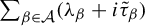 $\sum _{ \beta \in \mathcal {A} }(\unicode{x3bb} _{\beta }+i\tilde \tau _\beta )$
, that is, the one corresponding to
$\sum _{ \beta \in \mathcal {A} }(\unicode{x3bb} _{\beta }+i\tilde \tau _\beta )$
, that is, the one corresponding to
 $k=d$
, is below the x-axis. Moreover, due to the fact that
$k=d$
, is below the x-axis. Moreover, due to the fact that
 $\tilde \tau _{\pi _1^{-1}(d)}=\tilde \tau _{\alpha }>0$
, the subinterval of J given by
$\tilde \tau _{\pi _1^{-1}(d)}=\tilde \tau _{\alpha }>0$
, the subinterval of J given by
 $\bigcup _{t\in [h_{\alpha }+\sum _{\beta \in \mathcal {A}}\tilde {\tau }_\beta ,h_{\alpha })} \phi _t(x_0)$
is fully below the x-axis. Hence, since
$\bigcup _{t\in [h_{\alpha }+\sum _{\beta \in \mathcal {A}}\tilde {\tau }_\beta ,h_{\alpha })} \phi _t(x_0)$
is fully below the x-axis. Hence, since
 $h_{\alpha }+\sum _{\beta \in \mathcal {A}}\tilde {\tau }_\beta =\tilde \tau _{\alpha }=\tilde \tau _{\pi _0^{-1}(1)}$
, the discontinuity of S corresponding to
$h_{\alpha }+\sum _{\beta \in \mathcal {A}}\tilde {\tau }_\beta =\tilde \tau _{\alpha }=\tilde \tau _{\pi _0^{-1}(1)}$
, the discontinuity of S corresponding to
 $k=d$
is the point
$k=d$
is the point
 $y_{d}$
given by
$y_{d}$
given by
 $$ \begin{align} y_{d}:=\phi_{\tilde\tau_{\pi_0^{-1}(1)}}(x_0). \end{align} $$
On the other hand, for every
 $k=2,\ldots ,d-1$
, the initial segment of the corresponding incoming separatrix lies above the x-axis, and, due to (4.1) (and by (4.4)), the first backward hit of the incoming separatrix via
$k=2,\ldots ,d-1$
, the initial segment of the corresponding incoming separatrix lies above the x-axis, and, due to (4.1) (and by (4.4)), the first backward hit of the incoming separatrix via
 $\psi $
is the point
$\psi $
is the point
 $$ \begin{align} y_k:=\phi_{t_k}(x_0) \quad \text{where } t_k:= \sum_{\pi_0(\beta)\le k}\tilde\tau_{\beta}. \end{align} $$
Notice that we can use the above notation also for
 $k=1$
, that is,
$k=1$
, that is,
 $t_1=\tilde \tau _{\pi _0^{-1}(1)}$
and
$t_1=\tilde \tau _{\pi _0^{-1}(1)}$
and
 $y_1=\phi _{t_1}(x_0)=y_d$
. Note that none of the formulas (4.3), (4.5), or (4.6) depend on
$y_1=\phi _{t_1}(x_0)=y_d$
. Note that none of the formulas (4.3), (4.5), or (4.6) depend on
 $\unicode{x3bb} $
.
$\unicode{x3bb} $
.
It remains to describe the zippered rectangles crossed by the horizontal orbit segment of any point
 $x\in J$
. Note that due to (4.1) and (4.2) the order of the points
$x\in J$
. Note that due to (4.1) and (4.2) the order of the points
 $y_k$
on J, counting upwards, is
$y_k$
on J, counting upwards, is
 $y_{d-1},y_{d-2},\ldots ,y_{3},y_{2},y_{d}$
. Assume first that
$y_{d-1},y_{d-2},\ldots ,y_{3},y_{2},y_{d}$
. Assume first that
 $x\in (y_{k+1},y_k)\subseteq J$
for some
$x\in (y_{k+1},y_k)\subseteq J$
for some
 $k\in \{2,\ldots ,d-2\}$
. Then the orbit segment starting at x given by the forward action of
$k\in \{2,\ldots ,d-2\}$
. Then the orbit segment starting at x given by the forward action of
 $\psi $
leaves the zippered rectangle
$\psi $
leaves the zippered rectangle
 $D_{\alpha }$
then goes through the cylinders
$D_{\alpha }$
then goes through the cylinders
 $D_{\pi _0^{-1}(\ell )}$
for
$D_{\pi _0^{-1}(\ell )}$
for
 $2\leq \ell \leq k+1$
, and inside the zippered rectangle
$2\leq \ell \leq k+1$
, and inside the zippered rectangle
 $D_{\pi _0^{-1}(k+1)}$
it crosses the edge given by the vertices
$D_{\pi _0^{-1}(k+1)}$
it crosses the edge given by the vertices
 $\sum _{ \pi _0(\beta )\le k}(\unicode{x3bb} _{\beta }+i\tilde \tau _\beta )$
and
$\sum _{ \pi _0(\beta )\le k}(\unicode{x3bb} _{\beta }+i\tilde \tau _\beta )$
and
 $\sum _{ \pi _0(\beta )\le k+1}(\unicode{x3bb} _{\beta }+i\tilde \tau _\beta )$
. This describes the part of the segment in the part of the polygonal representation above the x-axis. After crossing the side of the polygon, it goes through zippered rectangles
$\sum _{ \pi _0(\beta )\le k+1}(\unicode{x3bb} _{\beta }+i\tilde \tau _\beta )$
. This describes the part of the segment in the part of the polygonal representation above the x-axis. After crossing the side of the polygon, it goes through zippered rectangles
 $D_{\pi _1^{-1}(\ell )}$
, with
$D_{\pi _1^{-1}(\ell )}$
, with
 $\pi _1(\pi _0^{-1}(k+1))\leq \ell \leq d-1$
in the lower part of the polygon. After that, the orbit goes to
$\pi _1(\pi _0^{-1}(k+1))\leq \ell \leq d-1$
in the lower part of the polygon. After that, the orbit goes to
 $D_{\pi _1^{-1}(d)}=D_{\alpha }$
and returns directly to J. Hence, in the case when
$D_{\pi _1^{-1}(d)}=D_{\alpha }$
and returns directly to J. Hence, in the case when
 $x\in (y_{k+1},y_k)$
for some
$x\in (y_{k+1},y_k)$
for some
 $k\in \{2,\ldots ,d-2\}$
, the orbit crosses at most
$k\in \{2,\ldots ,d-2\}$
, the orbit crosses at most
 $2d-2$
edges of zippered rectangles different from
$2d-2$
edges of zippered rectangles different from
 $D_\alpha $
.
$D_\alpha $
.
To describe the horizontal orbit segment for
 $x\in (y_{2},y_{d})=(y_{2},y_{1})$
it suffices to take
$x\in (y_{2},y_{d})=(y_{2},y_{1})$
it suffices to take
 $k=1$
in the above description of the passage of the orbit through zippered rectangles.
$k=1$
in the above description of the passage of the orbit through zippered rectangles.
If
 $x\in (x_0,y_{d-1})$
then the orbit segment starting at x obtained by acting forward via
$x\in (x_0,y_{d-1})$
then the orbit segment starting at x obtained by acting forward via
 $\psi $
passes all zippered rectangles in the upper part of the polygonal representation of
$\psi $
passes all zippered rectangles in the upper part of the polygonal representation of
 $(\pi ,\unicode{x3bb} ,\tilde {\tau })$
, before crossing the edge given by
$(\pi ,\unicode{x3bb} ,\tilde {\tau })$
, before crossing the edge given by
 $\sum _{ \pi _0(\beta ) < d}(\unicode{x3bb} _{\beta }+i\tilde \tau _\beta )$
and
$\sum _{ \pi _0(\beta ) < d}(\unicode{x3bb} _{\beta }+i\tilde \tau _\beta )$
and
 $\sum _{\beta \in \mathcal {A}}(\unicode{x3bb} _{\beta }+i\tilde \tau _\beta )$
. Then, before returning to the zippered rectangle
$\sum _{\beta \in \mathcal {A}}(\unicode{x3bb} _{\beta }+i\tilde \tau _\beta )$
. Then, before returning to the zippered rectangle
 $D_{\alpha }$
it passes through the zippered rectangles
$D_{\alpha }$
it passes through the zippered rectangles
 $D_{\pi _1^{-1}(\ell )}$
, with
$D_{\pi _1^{-1}(\ell )}$
, with
 $\pi _1(\pi _0^{-1}(d))\leq \ell \leq d-1$
. After that, the orbit goes to
$\pi _1(\pi _0^{-1}(d))\leq \ell \leq d-1$
. After that, the orbit goes to
 $D_{\pi _1^{-1}(d)}=D_{\alpha }$
and returns directly to J. Hence, it also crosses no more than
$D_{\pi _1^{-1}(d)}=D_{\alpha }$
and returns directly to J. Hence, it also crosses no more than
 $2d-2$
edges of zippered rectangles different from
$2d-2$
edges of zippered rectangles different from
 $D_\alpha $
.
$D_\alpha $
.
Finally, if
 $x\in ({y_d}, \phi _{h_{\alpha }}(x_0))$
, then the orbit of x does not leave the lower part of the polygonal representation of
$x\in ({y_d}, \phi _{h_{\alpha }}(x_0))$
, then the orbit of x does not leave the lower part of the polygonal representation of
 $(\pi ,\unicode{x3bb} ,{\tilde \tau })$
before returning to
$(\pi ,\unicode{x3bb} ,{\tilde \tau })$
before returning to
 $D_{\alpha }$
. After leaving the zippered rectangle
$D_{\alpha }$
. After leaving the zippered rectangle
 $D_{\alpha }$
, it goes through zippered rectangles
$D_{\alpha }$
, it goes through zippered rectangles
 $D_{\pi _1^{-1}(\ell )}$
, with
$D_{\pi _1^{-1}(\ell )}$
, with
 $\pi _1(\pi _0^{-1}(d))+1\leq \ell \leq d-1$
(note that here, if
$\pi _1(\pi _0^{-1}(d))+1\leq \ell \leq d-1$
(note that here, if
 $\pi _1(\pi _0^{-1}(d))=d-1$
, then the set of the indices
$\pi _1(\pi _0^{-1}(d))=d-1$
, then the set of the indices
 $\ell '$
is empty, that is, the horizontal orbit of x does not leave
$\ell '$
is empty, that is, the horizontal orbit of x does not leave
 $D_{\alpha }$
before the first return to J). After that, the orbit goes to
$D_{\alpha }$
before the first return to J). After that, the orbit goes to
 $D_{\pi _1^{-1}(d)}=D_{\alpha }$
and returns directly to J. Hence, in this case, the horizontal orbit of x does not cross more than
$D_{\pi _1^{-1}(d)}=D_{\alpha }$
and returns directly to J. Hence, in this case, the horizontal orbit of x does not cross more than
 $d-1$
edges of zippered rectangles different from
$d-1$
edges of zippered rectangles different from
 $D_\alpha $
. Thus the thesis of the lemma holds for
$D_\alpha $
. Thus the thesis of the lemma holds for
 $(\pi ,\unicode{x3bb} ,\tilde {\tau })$
with
$(\pi ,\unicode{x3bb} ,\tilde {\tau })$
with
 $C=2d-2$
.
$C=2d-2$
.
Since the values in (4.3), (4.5) and (4.6) change continuously with respect to
 $\tilde \tau $
, we can find an
$\tilde \tau $
, we can find an
 $\epsilon>0$
such that the inequalities (4.1) and (4.2) hold for any
$\epsilon>0$
such that the inequalities (4.1) and (4.2) hold for any
 $\tau \in B_{\Theta _\pi }(\tilde \tau , \epsilon )$
and, in particular, the order in which the discontinuities coming from specific vertices appear on the vertical section remains unchanged. Hence, the order of visited zippered rectangles stays the same, and the thesis holds with
$\tau \in B_{\Theta _\pi }(\tilde \tau , \epsilon )$
and, in particular, the order in which the discontinuities coming from specific vertices appear on the vertical section remains unchanged. Hence, the order of visited zippered rectangles stays the same, and the thesis holds with
 $C=2d-2$
.
$C=2d-2$
.
Proof of Proposition 4.1
Fix
 $\tilde \tau \in \Theta _\pi $
and let
$\tilde \tau \in \Theta _\pi $
and let
 $\epsilon =\epsilon (\tilde \tau )$
and
$\epsilon =\epsilon (\tilde \tau )$
and
 $C=C(\tilde \tau ,\epsilon )$
be given by Lemma 4.2. Fix
$C=C(\tilde \tau ,\epsilon )$
be given by Lemma 4.2. Fix
 $\alpha \in \mathcal {A}$
and
$\alpha \in \mathcal {A}$
and
 $n\in \mathbb {N}$
such that
$n\in \mathbb {N}$
such that
 $\mathcal R^{n}(\pi ,\unicode{x3bb} ,\tau )\in \{\pi \}\times \mathbb {R}_{>0}^{\mathcal {A}}\times B_{\Theta _{\pi }}(\tilde \tau ,\epsilon )$
. Let
$\mathcal R^{n}(\pi ,\unicode{x3bb} ,\tau )\in \{\pi \}\times \mathbb {R}_{>0}^{\mathcal {A}}\times B_{\Theta _{\pi }}(\tilde \tau ,\epsilon )$
. Let
 $(\pi ,\unicode{x3bb} ^{(n)},\tau ^{(n)})=R^{n}(\pi ,\unicode{x3bb} ,\tau )$
. Then
$(\pi ,\unicode{x3bb} ^{(n)},\tau ^{(n)})=R^{n}(\pi ,\unicode{x3bb} ,\tau )$
. Then
 $\mathcal R^{n}(\pi ,\unicode{x3bb} ,\tau )=(\pi ,e^s\unicode{x3bb} ^{(n)},e^{-s}\tau ^{(n)})$
with
$\mathcal R^{n}(\pi ,\unicode{x3bb} ,\tau )=(\pi ,e^s\unicode{x3bb} ^{(n)},e^{-s}\tau ^{(n)})$
with
 $s= -{\log}\, |\unicode{x3bb} ^{(n)}|$
. Since
$s= -{\log}\, |\unicode{x3bb} ^{(n)}|$
. Since
 ${R}^n(\pi , \unicode{x3bb} , \tau )$
and
${R}^n(\pi , \unicode{x3bb} , \tau )$
and
 $(\pi , \unicode{x3bb} , \tau )$
describe the same surface, we can decompose the surface
$(\pi , \unicode{x3bb} , \tau )$
describe the same surface, we can decompose the surface
 $(\pi , \unicode{x3bb} , \tau )$
into zippered rectangles
$(\pi , \unicode{x3bb} , \tau )$
into zippered rectangles
 $\{D^{(n)}_\beta \,|\ \beta \in \mathcal {A}\}$
according to numerical data
$\{D^{(n)}_\beta \,|\ \beta \in \mathcal {A}\}$
according to numerical data
 $(\pi ,\unicode{x3bb} ^{(n)},\tau ^{(n)})$
, that is,
$(\pi ,\unicode{x3bb} ^{(n)},\tau ^{(n)})$
, that is,
 $D^{(n)}_\beta =\bigcup _{0\leq t<h^{(n)}_\beta }\phi _t I^{(n)}_\beta $
, where
$D^{(n)}_\beta =\bigcup _{0\leq t<h^{(n)}_\beta }\phi _t I^{(n)}_\beta $
, where
 $h^{(n)}=(h^{(n)}_\beta )_{\beta \in \mathcal {A}}=-\Omega _\pi \tau ^{(n)}$
. Then
$h^{(n)}=(h^{(n)}_\beta )_{\beta \in \mathcal {A}}=-\Omega _\pi \tau ^{(n)}$
. Then
 $T^jI^{(n)}_\beta =\phi _{t^\beta _j} I^{(n)}_\beta $
for
$T^jI^{(n)}_\beta =\phi _{t^\beta _j} I^{(n)}_\beta $
for
 $0\leq j\leq q^{(n)}_\beta $
, where
$0\leq j\leq q^{(n)}_\beta $
, where
 $0=t^\beta _0<t^\beta _1<\cdots <t^\beta _{q^{(n)}_\beta }=h^{(n)}_{\beta }$
are consecutive recurrence times of
$0=t^\beta _0<t^\beta _1<\cdots <t^\beta _{q^{(n)}_\beta }=h^{(n)}_{\beta }$
are consecutive recurrence times of
 $I^{(n)}_\beta $
to the interval I.
$I^{(n)}_\beta $
to the interval I.
Let
 $x\in T^m(I^{(n)}_{\alpha })$
for some
$x\in T^m(I^{(n)}_{\alpha })$
for some
 $0\leq m< q^{(n)}_\alpha $
. Consider
$0\leq m< q^{(n)}_\alpha $
. Consider
 $T^m(I^{(n)}_{\alpha })$
as a subset of the surface
$T^m(I^{(n)}_{\alpha })$
as a subset of the surface
 $(\pi ,\unicode{x3bb} ,\tau )$
and let J be a vertical segment of length
$(\pi ,\unicode{x3bb} ,\tau )$
and let J be a vertical segment of length
 $h_{\alpha }^{(n)}$
inside
$h_{\alpha }^{(n)}$
inside
 $D_{\alpha }^{(n)}$
, which starts at
$D_{\alpha }^{(n)}$
, which starts at
 $I_{\alpha }^{(n)}$
(at
$I_{\alpha }^{(n)}$
(at
 $x_0=T^{-m}x$
), which contains x. As
$x_0=T^{-m}x$
), which contains x. As
 $R^n(\pi , \unicode{x3bb} , \tau )$
is obtained from
$R^n(\pi , \unicode{x3bb} , \tau )$
is obtained from
 $\mathcal {R}^n(\pi , \unicode{x3bb} , \tau )$
by vertical and horizontal rescaling, they have the same (up to rescaling) decompositions into zippered rectangles. As
$\mathcal {R}^n(\pi , \unicode{x3bb} , \tau )$
by vertical and horizontal rescaling, they have the same (up to rescaling) decompositions into zippered rectangles. As
 $\mathcal R^{n}(\pi ,\unicode{x3bb} ,\tau )\in \{\pi \}\times \mathbb {R}_{>0}^{\mathcal {A}}\times B_{\Theta _{\pi }}(\tilde \tau ,\epsilon )$
, in view of Lemma 4.2 and denoting by r the first return time of x to J via the horizontal flow
$\mathcal R^{n}(\pi ,\unicode{x3bb} ,\tau )\in \{\pi \}\times \mathbb {R}_{>0}^{\mathcal {A}}\times B_{\Theta _{\pi }}(\tilde \tau ,\epsilon )$
, in view of Lemma 4.2 and denoting by r the first return time of x to J via the horizontal flow
 $\psi $
, the orbit
$\psi $
, the orbit
 $(\psi _{t}(x))_{t\in (0,r)}$
crosses at most C edges of the zippered rectangles
$(\psi _{t}(x))_{t\in (0,r)}$
crosses at most C edges of the zippered rectangles
 $D^{(n)}_\beta $
,
$D^{(n)}_\beta $
,
 $\beta \in \mathcal {A}\setminus \{\alpha \}$
before returning to
$\beta \in \mathcal {A}\setminus \{\alpha \}$
before returning to
 $J\subset D^{(n)}_\alpha $
. In particular,
$J\subset D^{(n)}_\alpha $
. In particular,
 $\psi _{r}(x)\in J\subset D^{(n)}_\alpha $
.
$\psi _{r}(x)\in J\subset D^{(n)}_\alpha $
.
There are two possibilities: either
 $(\psi _{t}(x))_{t\in (0,r)}$
is not included in I, which is equivalent to the fact that
$(\psi _{t}(x))_{t\in (0,r)}$
is not included in I, which is equivalent to the fact that
 $T^m(I^{(n)}_{\alpha })$
is the rightmost level of the tower
$T^m(I^{(n)}_{\alpha })$
is the rightmost level of the tower
 $\bigcup _{j=0}^{q^{(n)}_\alpha -1}T^j(I^{(n)}_{\alpha })$
with respect to the linear order on I, or
$\bigcup _{j=0}^{q^{(n)}_\alpha -1}T^j(I^{(n)}_{\alpha })$
with respect to the linear order on I, or
 $(\psi _{t}(x))_{t\in (0,r)}$
is a subinterval of I. Indeed, if x does not belong to the rightmost level of the tower
$(\psi _{t}(x))_{t\in (0,r)}$
is a subinterval of I. Indeed, if x does not belong to the rightmost level of the tower
 $\bigcup _{j=0}^{q^{(n)}_\alpha -1}T^j(I^{(n)}_{\alpha })$
, then denote by
$\bigcup _{j=0}^{q^{(n)}_\alpha -1}T^j(I^{(n)}_{\alpha })$
, then denote by
 $T^{m'}(I^{(n)}_{\alpha })$
the next level traveling horizontally. Then
$T^{m'}(I^{(n)}_{\alpha })$
the next level traveling horizontally. Then
 $\psi _r(x)\in T^{m'}(I^{(n)}_{\alpha })\subset I$
. It follows that the horizontal interval
$\psi _r(x)\in T^{m'}(I^{(n)}_{\alpha })\subset I$
. It follows that the horizontal interval
 $(\psi _{t}(x))_{t\in (0,r)}$
is a subinterval of I.
$(\psi _{t}(x))_{t\in (0,r)}$
is a subinterval of I.
Let us assume first that
 $(\psi _{t}(x))_{t\in (0,r)} \subseteq I$
. Recall that for any
$(\psi _{t}(x))_{t\in (0,r)} \subseteq I$
. Recall that for any
 $\beta \in \mathcal {A}$
, the tower
$\beta \in \mathcal {A}$
, the tower
 $\bigcup _{j=0}^{q^{(n)}_\beta -1}{T^j(I^{(n)}_\beta )}$
is fully included inside the zippered rectangle
$\bigcup _{j=0}^{q^{(n)}_\beta -1}{T^j(I^{(n)}_\beta )}$
is fully included inside the zippered rectangle
 $D_{\beta }^{(n)}$
. Hence, the fact that
$D_{\beta }^{(n)}$
. Hence, the fact that
 $(\psi _{t}(x))_{t\in (0,r)}$
crosses at most C times the edges of zippered rectangles is equivalent to the fact that it crosses at most C times the endpoints of levels of towers corresponding to other symbols than
$(\psi _{t}(x))_{t\in (0,r)}$
crosses at most C times the edges of zippered rectangles is equivalent to the fact that it crosses at most C times the endpoints of levels of towers corresponding to other symbols than
 $\alpha $
. Moreover, since
$\alpha $
. Moreover, since
 $\psi _r(x)\in T^{m'}(I^{(n)}_\alpha )$
(this is the next level of the tower traveling horizontally), the interval between
$\psi _r(x)\in T^{m'}(I^{(n)}_\alpha )$
(this is the next level of the tower traveling horizontally), the interval between
 $T^{m}(I^{(n)}_\alpha )$
and
$T^{m}(I^{(n)}_\alpha )$
and
 $T^{m'}(I^{(n)}_\alpha )$
contains at most C levels of towers other than
$T^{m'}(I^{(n)}_\alpha )$
contains at most C levels of towers other than
 $\bigcup _{j=0}^{q^{(n)}_\alpha -1}T^j(I^{(n)}_{\alpha })$
.
$\bigcup _{j=0}^{q^{(n)}_\alpha -1}T^j(I^{(n)}_{\alpha })$
.
If, on the other hand, we have
 $(\psi _{t}(x))_{t\in (0,r)} \not \subseteq I$
, then
$(\psi _{t}(x))_{t\in (0,r)} \not \subseteq I$
, then
 $(\psi _{t}(x))_{t\in (0,r)}$
contains the right-hand-side endpoint of I and hence contains the rightmost interval in
$(\psi _{t}(x))_{t\in (0,r)}$
contains the right-hand-side endpoint of I and hence contains the rightmost interval in
 $I\setminus \bigsqcup _{j=0}^{q_{\alpha }^{(n)}-1}T^jI^{(n)}_\alpha $
. As
$I\setminus \bigsqcup _{j=0}^{q_{\alpha }^{(n)}-1}T^jI^{(n)}_\alpha $
. As
 $(\psi _{t}(x))_{t\in (0,r)}$
crosses at most C edges of the zippered rectangles
$(\psi _{t}(x))_{t\in (0,r)}$
crosses at most C edges of the zippered rectangles
 $D^{(n)}_\beta $
,
$D^{(n)}_\beta $
,
 $\beta \in \mathcal {A}\setminus \{\alpha \}$
, the argument used in the previous paragraph shows that the rightmost interval in
$\beta \in \mathcal {A}\setminus \{\alpha \}$
, the argument used in the previous paragraph shows that the rightmost interval in
 $I\setminus \bigsqcup _{j=0}^{q_{\alpha }^{(n)}-1}T^jI^{(n)}_\alpha $
contains at most C levels of towers other than
$I\setminus \bigsqcup _{j=0}^{q_{\alpha }^{(n)}-1}T^jI^{(n)}_\alpha $
contains at most C levels of towers other than
 $\bigcup _{j=0}^{q^{(n)}_\alpha -1}T^j(I^{(n)}_{\alpha })$
.
$\bigcup _{j=0}^{q^{(n)}_\alpha -1}T^j(I^{(n)}_{\alpha })$
.
It remains to consider the leftmost component of
 $I\setminus \bigsqcup _{j=0}^{q_{\alpha }^{(n)}-1}T^jI^{(n)}_\alpha $
, with respect to the linear order on I. This is done by choosing a point x in the intersection of J and the leftmost level of
$I\setminus \bigsqcup _{j=0}^{q_{\alpha }^{(n)}-1}T^jI^{(n)}_\alpha $
, with respect to the linear order on I. This is done by choosing a point x in the intersection of J and the leftmost level of
 $\bigsqcup _{j=0}^{q_{\alpha }^{(n)}-1}T^jI^{(n)}_\alpha $
and taking
$\bigsqcup _{j=0}^{q_{\alpha }^{(n)}-1}T^jI^{(n)}_\alpha $
and taking
 $r_0\geq 0$
such that
$r_0\geq 0$
such that
 $\psi _{-r_0}(x)=0$
is the left endpoint of I. Then the orbit
$\psi _{-r_0}(x)=0$
is the left endpoint of I. Then the orbit
 $(\psi _{-t}(x))_{t\in (0,r_0)}$
contains the leftmost component of
$(\psi _{-t}(x))_{t\in (0,r_0)}$
contains the leftmost component of
 $I\setminus \bigsqcup _{j=0}^{q_{\alpha }^{(n)}-1}T^jI^{(n)}_\alpha $
. Next, choose
$I\setminus \bigsqcup _{j=0}^{q_{\alpha }^{(n)}-1}T^jI^{(n)}_\alpha $
. Next, choose
 $x_\delta =\phi _\delta x\in J$
for small enough
$x_\delta =\phi _\delta x\in J$
for small enough
 $\delta>0$
. Let
$\delta>0$
. Let
 $y=\psi _{-r}x_\delta \in J$
be the first backward return point for the horizontal flow to J. For all
$y=\psi _{-r}x_\delta \in J$
be the first backward return point for the horizontal flow to J. For all
 $\delta>0$
small enough, we have
$\delta>0$
small enough, we have
 $r>r_0$
. In view of Lemma 4.2, the orbit
$r>r_0$
. In view of Lemma 4.2, the orbit
 $(\psi _{t}(y))_{t\in (0,r)}=(\psi _{-t}(x_\delta ))_{t\in (0,r)}$
crosses at most C edges of the zippered rectangles
$(\psi _{t}(y))_{t\in (0,r)}=(\psi _{-t}(x_\delta ))_{t\in (0,r)}$
crosses at most C edges of the zippered rectangles
 $D^{(n)}_\beta $
,
$D^{(n)}_\beta $
,
 $\beta \in \mathcal {A}\setminus \{\alpha \}$
. As
$\beta \in \mathcal {A}\setminus \{\alpha \}$
. As
 $r>r_0$
, the orbit
$r>r_0$
, the orbit
 $(\psi _{-t}(x_\delta ))_{t\in (0,r_0)}$
, and hence the
$(\psi _{-t}(x_\delta ))_{t\in (0,r_0)}$
, and hence the
 $\delta $
-close orbit
$\delta $
-close orbit
 $(\psi _{-t}(x))_{t\in (0,r_0)}$
, crosses at most C edges of the zippered rectangles
$(\psi _{-t}(x))_{t\in (0,r_0)}$
, crosses at most C edges of the zippered rectangles
 $D^{(n)}_\beta $
,
$D^{(n)}_\beta $
,
 $\beta \in \mathcal {A}\setminus \{\alpha \}$
. Finally, the argument used in the previous paragraphs shows that the leftmost interval in
$\beta \in \mathcal {A}\setminus \{\alpha \}$
. Finally, the argument used in the previous paragraphs shows that the leftmost interval in
 $I\setminus \bigsqcup _{j=0}^{q_{\alpha }^{(n)}-1}T^jI^{(n)}_\alpha $
contains at most C levels of towers other than
$I\setminus \bigsqcup _{j=0}^{q_{\alpha }^{(n)}-1}T^jI^{(n)}_\alpha $
contains at most C levels of towers other than
 $\bigcup _{j=0}^{q^{(n)}_\alpha -1}T^j(I^{(n)}_{\alpha })$
. This completes the proof of the proposition.
$\bigcup _{j=0}^{q^{(n)}_\alpha -1}T^j(I^{(n)}_{\alpha })$
. This completes the proof of the proposition.
5 Diophantine conditions
In this section, we show that a certain collection of properties holds for typical IETs. These properties concern the parametric description of properly chosen return sets for the Zorich induction
 $\mathcal Z$
. For an overview of the history and recent development of techniques related to different types of Diophantine properties for IETs and translation surfaces, we refer to the survey paper [Reference Ulcigrai25].
$\mathcal Z$
. For an overview of the history and recent development of techniques related to different types of Diophantine properties for IETs and translation surfaces, we refer to the survey paper [Reference Ulcigrai25].
Fix a Rauzy graph
 $\mathcal G\subset S^{\mathcal {A}}$
and consider an IET
$\mathcal G\subset S^{\mathcal {A}}$
and consider an IET
 $(\pi ,\unicode{x3bb} )$
such that
$(\pi ,\unicode{x3bb} )$
such that
 $\pi \in \mathcal G$
is an irreducible permutation over an alphabet
$\pi \in \mathcal G$
is an irreducible permutation over an alphabet
 $\mathcal {A}$
of
$\mathcal {A}$
of
 $d\ge 2$
elements. Assume that there exist an increasing sequence
$d\ge 2$
elements. Assume that there exist an increasing sequence
 $\{q_n\}_{n\in \mathbb {N}}$
of natural numbers, a sequence
$\{q_n\}_{n\in \mathbb {N}}$
of natural numbers, a sequence
 $\{\{T^i(\Delta ^{n}) \mid 0\leq i<q_n\}\}_{n\in \mathbb {N}}$
of Rokhlin towers, and a constant
$\{\{T^i(\Delta ^{n}) \mid 0\leq i<q_n\}\}_{n\in \mathbb {N}}$
of Rokhlin towers, and a constant
 $C>1$
, such that
$C>1$
, such that
 $$ \begin{align} \limsup_{n\to\infty}(q_n)^{{1}/{n}}<\infty; \end{align} $$
and, for any
 $n \in \mathbb {N}$
,
$n \in \mathbb {N}$
,
 $$ \begin{align} q_{n+1}&\geq 320C^2 q_n, \end{align} $$
 $$ \begin{align} C&\geq q_n|\Delta^n|\geq C^{-1}>0, \end{align} $$
 $$ \begin{align} T^i(\Delta^n) \text{ is an interval disjoint from the discontinuities of } T, \text{ for any } 0 \leq i < q_n, \end{align} $$
 $$ \begin{align} &\bigg(\bigcup_{0\leq i<q_n}T^i(\Delta^n)\bigg)^c\text{ consists of at most } q_{n}+1 \text{ intervals (holes) of lengths less than } \dfrac{C}{q_n}, \end{align} $$
 $$ \begin{align} & \qquad\qquad T^{q_n}{\mid}_{\Delta^n} \text{ is a translation by a number from } (\tfrac{1}{16}|\Delta^n|,\tfrac{1}{8}|\Delta^n|). \end{align} $$
The allowed translation values described in (5.6) are given up to an absolute value. However, in the proof of the following proposition, the translations are exclusively to the left.
Proposition 5.1. For almost every
 $\unicode{x3bb} \in \Lambda ^{\mathcal A}$
there exist an increasing sequence
$\unicode{x3bb} \in \Lambda ^{\mathcal A}$
there exist an increasing sequence
 $\{q_n\}_{n\in \mathbb {N}}$
of natural numbers and a sequence
$\{q_n\}_{n\in \mathbb {N}}$
of natural numbers and a sequence
 $\{T^i(\Delta ^n) \mid 0\leq i<q_n\}_{n\in \mathbb {N}}$
of Rokhlin towers satisfying (5.2)–(5.6). Moreover, these conditions are obtained via returning to an appropriate subset
$\{T^i(\Delta ^n) \mid 0\leq i<q_n\}_{n\in \mathbb {N}}$
of Rokhlin towers satisfying (5.2)–(5.6). Moreover, these conditions are obtained via returning to an appropriate subset
 $\mathfrak L\subseteq \mathcal M$
of positive measure.
$\mathfrak L\subseteq \mathcal M$
of positive measure.
Proof. Fix
 $\pi \in S^{\mathcal {A}}$
and let
$\pi \in S^{\mathcal {A}}$
and let
 $\tau \in \Theta _{\pi }$
be rationally independent. We will choose an appropriate subset on which to induce the Zorich induction
$\tau \in \Theta _{\pi }$
be rationally independent. We will choose an appropriate subset on which to induce the Zorich induction
 $\mathcal Z$
. We will define
$\mathcal Z$
. We will define
 $\Delta^n$
as a properly chosen subinterval of the base of the tower
$\Delta^n$
as a properly chosen subinterval of the base of the tower
 $\bigcup _{j=0}^{q_\alpha^{(n)}-1}T^j(I^{(n)}_{\alpha })$
, for some
$\bigcup _{j=0}^{q_\alpha^{(n)}-1}T^j(I^{(n)}_{\alpha })$
, for some
 $\alpha \in \mathcal {A}$
.
$\alpha \in \mathcal {A}$
.
Let
 $\mathcal D_1\subseteq \Lambda ^{\mathcal {A}}$
be a set of length parameters such that
$\mathcal D_1\subseteq \Lambda ^{\mathcal {A}}$
be a set of length parameters such that
 $$ \begin{align} \mathcal D_1:=\{\unicode{x3bb}\in \Lambda^{\mathcal{A}}\mid \unicode{x3bb}_{\pi_0^{-1}(d)}\ge \tfrac{7}{8} \text{ and } \tfrac{1}{16}<|w_{\pi_0^{-1}(d)}|< \tfrac{1}{10} \}, \end{align} $$
where
 $w = \Omega _\pi \unicode{x3bb} $
is the translation vector associated with
$w = \Omega _\pi \unicode{x3bb} $
is the translation vector associated with
 $(\pi , \unicode{x3bb} )$
.
$(\pi , \unicode{x3bb} )$
.
Note that since
 $\unicode{x3bb} _{\pi _0^{-1}(d)}\ge \tfrac {7}{8}$
for
$\unicode{x3bb} _{\pi _0^{-1}(d)}\ge \tfrac {7}{8}$
for
 $\unicode{x3bb} \in \mathcal D_1$
, the IET
$\unicode{x3bb} \in \mathcal D_1$
, the IET
 $(\pi ,\unicode{x3bb} )$
has top type for the Rauzy–Veech induction. Moreover, whenever
$(\pi ,\unicode{x3bb} )$
has top type for the Rauzy–Veech induction. Moreover, whenever
 $\mathcal Z^n(\pi ,\unicode{x3bb} , \tau )\in \{\pi \}\times \mathcal D_1\times \Theta _{\pi }$
, we have that
$\mathcal Z^n(\pi ,\unicode{x3bb} , \tau )\in \{\pi \}\times \mathcal D_1\times \Theta _{\pi }$
, we have that
 $T^{q^{(n)}_{\pi _0^{-1}(d)}}$
acts on
$T^{q^{(n)}_{\pi _0^{-1}(d)}}$
acts on
 $I_{\pi _0^{-1}(d)}^{(n)}$
via translation by a number between
$I_{\pi _0^{-1}(d)}^{(n)}$
via translation by a number between
 $\tfrac {1}{16}|I_{\pi _0^{-1}(d)}^{(n)}|$
and
$\tfrac {1}{16}|I_{\pi _0^{-1}(d)}^{(n)}|$
and
 $\tfrac {1}{8}|I_{\pi _0^{-1}(d)}^{(n)}|$
. Thus, the interval
$\tfrac {1}{8}|I_{\pi _0^{-1}(d)}^{(n)}|$
. Thus, the interval
 $I_{\pi _0^{-1}(d)}^{(n)}$
satisfies (5.6).
$I_{\pi _0^{-1}(d)}^{(n)}$
satisfies (5.6).
Now let
 $\tilde \tau \in \Theta _{\pi }$
be such that
$\tilde \tau \in \Theta _{\pi }$
be such that
 $(\pi ,\unicode{x3bb} ,\tilde \tau )$
is of bottom backward type and
$(\pi ,\unicode{x3bb} ,\tilde \tau )$
is of bottom backward type and
 $\tilde \tau $
is rationally independent. Let
$\tilde \tau $
is rationally independent. Let
 $\epsilon =\epsilon (\tilde \tau )>0$
and
$\epsilon =\epsilon (\tilde \tau )>0$
and
 $C_1=C(\tilde \tau ,\epsilon )>0$
be given by Proposition 4.1. Denote
$C_1=C(\tilde \tau ,\epsilon )>0$
be given by Proposition 4.1. Denote
 $$ \begin{align*} \mathcal E:= \mathbb{R}_{>0}B_{\Theta_\pi}(\tilde\tau,\epsilon). \end{align*} $$
In view of Proposition 4.1, whenever
 $\mathcal Z^n(\pi ,\unicode{x3bb} ,\tau )\in \{\pi \}\times \mathcal D_1\times \mathcal E$
, the tower
$\mathcal Z^n(\pi ,\unicode{x3bb} ,\tau )\in \{\pi \}\times \mathcal D_1\times \mathcal E$
, the tower
 $\bigcup _{j=0}^{q^{(n)}_{\pi _0^{-1}(d)}-1} T^j {I_{\pi _0^{-1}(d)}^{(n)}}$
satisfies (5.5) with
$\bigcup _{j=0}^{q^{(n)}_{\pi _0^{-1}(d)}-1} T^j {I_{\pi _0^{-1}(d)}^{(n)}}$
satisfies (5.5) with
 $C=C_1$
. Moreover, since the cone
$C=C_1$
. Moreover, since the cone
 $\mathcal E$
is relatively compact (with respect to the Hilbert pseudometric) in
$\mathcal E$
is relatively compact (with respect to the Hilbert pseudometric) in
 $\Theta _{\pi }$
and by considering smaller
$\Theta _{\pi }$
and by considering smaller
 $\epsilon $
if necessary, we may assume that all
$\epsilon $
if necessary, we may assume that all
 $\tau \in \mathcal E$
are of bottom backward type and
$\tau \in \mathcal E$
are of bottom backward type and
 $$ \begin{align*} \sup_{\tau\in\mathcal E}\max_{\alpha,\beta\in \mathcal{A}}\frac{h_{\alpha}}{h_{\beta}} \leq C_2, \end{align*} $$
for some
 $C_2>0$
, where
$C_2>0$
, where
 $h=h(\tau )=-\Omega _{\pi }\tau $
is the height vector. It follows that if
$h=h(\tau )=-\Omega _{\pi }\tau $
is the height vector. It follows that if
 $\mathcal Z^n(\pi ,\unicode{x3bb} ,\tau )\in \{\pi \}\times \mathcal D_1\times \mathcal E$
, then
$\mathcal Z^n(\pi ,\unicode{x3bb} ,\tau )\in \{\pi \}\times \mathcal D_1\times \mathcal E$
, then
 $$ \begin{align*} \max_{\alpha,\beta\in \mathcal{A}}\frac{h^{(n)}_{\alpha}}{h^{(n)}_{\beta}} \leq C_2. \end{align*} $$
For every
 $\tau \in \Theta _\pi $
, let
$\tau \in \Theta _\pi $
, let
 $M(\tau ):=\max _{\alpha \in \mathcal {A}}h_\alpha (\tau )$
,
$M(\tau ):=\max _{\alpha \in \mathcal {A}}h_\alpha (\tau )$
,
 $m(\tau ):=\min _{\alpha \in \mathcal {A}}h_\alpha (\tau )$
and
$m(\tau ):=\min _{\alpha \in \mathcal {A}}h_\alpha (\tau )$
and
 $\delta (\tau ):={M(\tau )}/{m(\tau )}$
. As the zippered rectangle
$\delta (\tau ):={M(\tau )}/{m(\tau )}$
. As the zippered rectangle
 $D_\alpha ^{(n)}$
consists of
$D_\alpha ^{(n)}$
consists of
 $q_\alpha ^{(n)}$
rectangles of heights
$q_\alpha ^{(n)}$
rectangles of heights
 $h_\beta $
for
$h_\beta $
for
 $\beta \in \mathcal {A}$
, we have
$\beta \in \mathcal {A}$
, we have
 $$ \begin{align*}m(\tau)\leq \frac{h^{(n)}_{\alpha}}{q^{(n)}_{\alpha}}\leq M(\tau)\quad\text{for any }\alpha\in \mathcal{A}.\end{align*} $$
It follows that if
 $\mathcal Z^n(\pi ,\unicode{x3bb} ,\tau )\in \{\pi \}\times \mathcal D_1\times \mathcal E$
, then
$\mathcal Z^n(\pi ,\unicode{x3bb} ,\tau )\in \{\pi \}\times \mathcal D_1\times \mathcal E$
, then
 ${q^{(n)}_{\beta }}/{q^{(n)}_{\alpha }} \leq C_2\delta (\tau )$
for all
${q^{(n)}_{\beta }}/{q^{(n)}_{\alpha }} \leq C_2\delta (\tau )$
for all
 $\alpha , \beta \in \mathcal {A}$
, and, letting
$\alpha , \beta \in \mathcal {A}$
, and, letting
 $\alpha =\pi _0^{-1}(d)$
, we have
$\alpha =\pi _0^{-1}(d)$
, we have
 $$ \begin{align*} 1\hspace{-1pt}=\hspace{-1pt}|I|=\!\sum_{\beta\in\mathcal{A}}q^{(n)}_\beta|I^{(n)}_\beta|\hspace{-1pt}\leq\hspace{-1pt} C_2\delta(\tau)q^{(n)}_\alpha\!\sum_{\beta\in\mathcal{A}}|I^{(n)}_\beta|=C_2\delta(\tau)q^{(n)}_\alpha|I^{(n)}|\leq \frac{8}{7}C_2\delta(\tau)q^{(n)}_\alpha|I^{(n)}_\alpha|. \end{align*} $$
By taking
 $C:=\max \{C_1,\tfrac 87C_2\delta (\tau )\}$
, both conditions (5.3) and (5.5) are satisfied.
$C:=\max \{C_1,\tfrac 87C_2\delta (\tau )\}$
, both conditions (5.3) and (5.5) are satisfied.
By [Reference Marmi, Moussa and Yoccoz18] (see §1.2.4), for almost every
 $\unicode{x3bb} \in \mathcal {D}_1$
, there exists
$\unicode{x3bb} \in \mathcal {D}_1$
, there exists
 $k=k(\pi ,\unicode{x3bb} )\in \mathbb {N}$
such that the Kontsevich–Zorich matrix
$k=k(\pi ,\unicode{x3bb} )\in \mathbb {N}$
such that the Kontsevich–Zorich matrix
 $Q(k)(\pi ,\unicode{x3bb} )$
is positive (note that this matrix does not depend on
$Q(k)(\pi ,\unicode{x3bb} )$
is positive (note that this matrix does not depend on
 $\tau $
). Using the same argument for successive iterations of Zorich induction and multiplying several matrices with positive (natural) coefficients, for almost every
$\tau $
). Using the same argument for successive iterations of Zorich induction and multiplying several matrices with positive (natural) coefficients, for almost every
 $\unicode{x3bb} \in \mathcal {D}_1$
we can find
$\unicode{x3bb} \in \mathcal {D}_1$
we can find
 $N=N(\pi ,\unicode{x3bb} )\in \mathbb {N}$
such that all coefficients of the Kontsevich–Zorich matrix
$N=N(\pi ,\unicode{x3bb} )\in \mathbb {N}$
such that all coefficients of the Kontsevich–Zorich matrix
 $Q(N)(\pi ,\unicode{x3bb} )$
are greater than
$Q(N)(\pi ,\unicode{x3bb} )$
are greater than
 $320C^2$
. Since the Zorich induction
$320C^2$
. Since the Zorich induction
 $\mathcal Z$
and the Kontsevich–Zorich cocycle are locally continuous, there exists a subset
$\mathcal Z$
and the Kontsevich–Zorich cocycle are locally continuous, there exists a subset
 $\mathcal D_2\subseteq \mathcal D_1$
of positive measure such that the matrix
$\mathcal D_2\subseteq \mathcal D_1$
of positive measure such that the matrix
 $Q(N)$
is constant on
$Q(N)$
is constant on
 $\{\pi \}\times \mathcal D_2$
and all its coefficients are greater than
$\{\pi \}\times \mathcal D_2$
and all its coefficients are greater than
 $320C^2$
. Next, by the ergodicity of
$320C^2$
. Next, by the ergodicity of
 $\mathcal Z$
on
$\mathcal Z$
on
 $\mathcal M^1$
, there exists a subset
$\mathcal M^1$
, there exists a subset
 $\mathcal D_3\subseteq \mathcal D_2$
of positive measure such that
$\mathcal D_3\subseteq \mathcal D_2$
of positive measure such that
 $\mathcal Z^{j}(\{\pi \}\times \mathcal D_3\times \Theta _\pi )$
are pairwise disjoint for
$\mathcal Z^{j}(\{\pi \}\times \mathcal D_3\times \Theta _\pi )$
are pairwise disjoint for
 $0\leq j\leq N$
. Thus, if
$0\leq j\leq N$
. Thus, if
 $\mathcal Z^{n_k}(\pi ,\unicode{x3bb} ,\tau ),\mathcal Z^{n_{k+1}}(\pi ,\unicode{x3bb} ,\tau )\in \{\pi \}\times \mathcal D_3\times \mathcal E$
are two consecutive visits
$\mathcal Z^{n_k}(\pi ,\unicode{x3bb} ,\tau ),\mathcal Z^{n_{k+1}}(\pi ,\unicode{x3bb} ,\tau )\in \{\pi \}\times \mathcal D_3\times \mathcal E$
are two consecutive visits
 $\{\pi \}\times \mathcal D_3\times \mathcal E$
, then
$\{\pi \}\times \mathcal D_3\times \mathcal E$
, then
 $q^{(k_{n+1})}_\alpha \geq 320C^2q^{(k_{n})}_\alpha $
for any
$q^{(k_{n+1})}_\alpha \geq 320C^2q^{(k_{n})}_\alpha $
for any
 $\alpha \in \mathcal {A}$
ensuring that condition (5.2) is met. Summarizing, by taking
$\alpha \in \mathcal {A}$
ensuring that condition (5.2) is met. Summarizing, by taking
 $$ \begin{align*} \Delta^n:=I_{\pi_0^{-1}(d)}^{(k_n)}\quad\text{and}\quad q_n:=q^{(k_n)}_{\pi_0^{-1}(d)}, \end{align*} $$
where
 $k_n:=k_n(\pi ,\unicode{x3bb} ,\tau )$
is such that
$k_n:=k_n(\pi ,\unicode{x3bb} ,\tau )$
is such that
 $k_n$
is the nth visit of
$k_n$
is the nth visit of
 $(\pi ,\unicode{x3bb} ,\tau )$
in
$(\pi ,\unicode{x3bb} ,\tau )$
in
 $\mathfrak L:=\{\pi \}\times \mathcal D_3\times \mathcal E$
, we obtain that (5.2)–(5.6) are satisfied and the proof is complete.
$\mathfrak L:=\{\pi \}\times \mathcal D_3\times \mathcal E$
, we obtain that (5.2)–(5.6) are satisfied and the proof is complete.
Remark 5.2. If we assume additionally that the permutation
 $\pi $
is symmetric and
$\pi $
is symmetric and
 $\tau $
in the beginning of the proof of Proposition 5.1 is chosen so that
$\tau $
in the beginning of the proof of Proposition 5.1 is chosen so that
 $$ \begin{align} \sum_{\alpha\in\mathcal{A}}\tau_{\alpha}>0>\sum_{\alpha\in \mathcal{A}}\tau_{\alpha}-\dfrac{1}{2}\tau_{\pi_1^{-1}(d)}, \end{align} $$
then by choosing
 $\mathcal E$
so that all elements of
$\mathcal E$
so that all elements of
 $\mathcal E$
satisfy this condition and by Lemma 3.12 and Remark 4 in [Reference Berk, Trujillo and Ulcigrai3] we get that
$\mathcal E$
satisfy this condition and by Lemma 3.12 and Remark 4 in [Reference Berk, Trujillo and Ulcigrai3] we get that
 $\tfrac {1}{2}$
and the midpoints
$\tfrac {1}{2}$
and the midpoints
 $m_{\alpha }$
of the intervals
$m_{\alpha }$
of the intervals
 $I_{\alpha }$
are forward images of the midpoints of the interval
$I_{\alpha }$
are forward images of the midpoints of the interval
 $I^{(k_n)}$
or intervals
$I^{(k_n)}$
or intervals
 $I_{\alpha }^{(k_n)}$
. It follows also from the construction in [Reference Berk, Trujillo and Ulcigrai3] that if we also assume about
$I_{\alpha }^{(k_n)}$
. It follows also from the construction in [Reference Berk, Trujillo and Ulcigrai3] that if we also assume about
 $\tau $
that
$\tau $
that
 $$ \begin{align} \sum_{\alpha\in\mathcal{A}}\tau_{\alpha}< \sum_{\alpha\mid\pi_0(\alpha)\le k}\tau_{\alpha} \quad \text{for } k=1,\ldots,d-1, \end{align} $$
and
 $r\ge 0$
is such that the rth iteration of the midpoint of
$r\ge 0$
is such that the rth iteration of the midpoint of
 $I^{(k_n)}$
is either
$I^{(k_n)}$
is either
 $\tfrac {1}{2}$
or
$\tfrac {1}{2}$
or
 $m_{\alpha }$
, then
$m_{\alpha }$
, then
 $T^j(I^{(k_n)})$
is a continuity interval for T for
$T^j(I^{(k_n)})$
is a continuity interval for T for
 $j=0,\ldots ,r$
.
$j=0,\ldots ,r$
.
The presented conditions on the returns of the IET via the Zorich induction
 $\mathcal Z$
yield the geometric picture used to prove Propositions 6.4 and 6.3. However, they give no information on the behavior of the Birkhoff sum of the considered cocycles and their derivatives. A problem of this nature has already been tackled by the second author and Corinna Ulcigrai in [Reference Frączek and Ulcigrai12]. There, the authors introduced two Diophantine conditions called the uniform Diophantine condition (UDC) and the symmetric uniform Diophantine condition (SUDC); see Definitions 3 and 7 in [Reference Frączek and Ulcigrai12]. For the sake of this paper, it is not important to recall their rather technical formal definitions. However, their consequences will be of considerable use. One of the crucial implications is that the UDC condition gives a sufficient condition for (5.1) to be satisfied for the heights of towers obtained by considering the renormalization times which satisfy the UDC condition.
$\mathcal Z$
yield the geometric picture used to prove Propositions 6.4 and 6.3. However, they give no information on the behavior of the Birkhoff sum of the considered cocycles and their derivatives. A problem of this nature has already been tackled by the second author and Corinna Ulcigrai in [Reference Frączek and Ulcigrai12]. There, the authors introduced two Diophantine conditions called the uniform Diophantine condition (UDC) and the symmetric uniform Diophantine condition (SUDC); see Definitions 3 and 7 in [Reference Frączek and Ulcigrai12]. For the sake of this paper, it is not important to recall their rather technical formal definitions. However, their consequences will be of considerable use. One of the crucial implications is that the UDC condition gives a sufficient condition for (5.1) to be satisfied for the heights of towers obtained by considering the renormalization times which satisfy the UDC condition.
To obtain the UDC and SUDC in [Reference Frączek and Ulcigrai12], the authors considered a proper inducing of the Kontsevich–Zorich cocycle to a subset K of positive measure in
 $\mathcal M^1$
(see Theorems 3.8 and 5.6 in [Reference Frączek and Ulcigrai12]). To adjust our conditions to theirs, we first consider a set
$\mathcal M^1$
(see Theorems 3.8 and 5.6 in [Reference Frączek and Ulcigrai12]). To adjust our conditions to theirs, we first consider a set
 $\mathfrak L$
from Proposition 5.1 with the recurrence set
$\mathfrak L$
from Proposition 5.1 with the recurrence set
 $\mathfrak D$
chosen in [Reference Ulcigrai24] to guarantee the control over the Birkhoff sums of the derivatives of logarithmic cocycles (see Lemmas 2.1 and 2.2 in [Reference Ulcigrai24]). In the proof of the first of the lemmas, the author uses Egorov’s theorem to obtain the desired set, while in the second, it is again a matter of choosing a sufficiently large defining constant. In particular, the recurrence set from [Reference Ulcigrai24] can be made arbitrarily large. Thus, we may assume that the set Y is constructed as an intersection of
$\mathfrak D$
chosen in [Reference Ulcigrai24] to guarantee the control over the Birkhoff sums of the derivatives of logarithmic cocycles (see Lemmas 2.1 and 2.2 in [Reference Ulcigrai24]). In the proof of the first of the lemmas, the author uses Egorov’s theorem to obtain the desired set, while in the second, it is again a matter of choosing a sufficiently large defining constant. In particular, the recurrence set from [Reference Ulcigrai24] can be made arbitrarily large. Thus, we may assume that the set Y is constructed as an intersection of
 $\mathfrak L$
, and this recurrence set
$\mathfrak L$
, and this recurrence set
 $\mathfrak D$
has a positive Lebesgue measure. Now it remains to take this set Y in Lemma 3.6 in [Reference Frączek and Ulcigrai12] and choose the set K in the proof of Theorem 3.8 as a subset of
$\mathfrak D$
has a positive Lebesgue measure. Now it remains to take this set Y in Lemma 3.6 in [Reference Frączek and Ulcigrai12] and choose the set K in the proof of Theorem 3.8 as a subset of
 $\mathfrak D\cap \mathfrak L$
. By now taking
$\mathfrak D\cap \mathfrak L$
. By now taking
 $\mathfrak L$
as the set which satisfies Proposition 5.1 (and Remark 5.2), we get the following proposition.
$\mathfrak L$
as the set which satisfies Proposition 5.1 (and Remark 5.2), we get the following proposition.
Proposition 5.3. Let
 $\pi \in S^{\mathcal A}$
. For almost every
$\pi \in S^{\mathcal A}$
. For almost every
 $T=(\pi ,\unicode{x3bb} )\in \{\pi \}\times \Lambda ^{\mathcal A}$
there exist an increasing sequence
$T=(\pi ,\unicode{x3bb} )\in \{\pi \}\times \Lambda ^{\mathcal A}$
there exist an increasing sequence
 $\{q_n\}_{n\in \mathbb {N}}$
of natural numbers and a sequence
$\{q_n\}_{n\in \mathbb {N}}$
of natural numbers and a sequence
 $\{\{T^i(\Delta ^n) \mid 0\leq i<q_n\}\}_{n\in \mathbb {N}}$
of Rokhlin towers satisfying (5.1)–(5.6). Moreover, the UDC and SUDC are satisfied for the sequence of renormalization times that yields
$\{\{T^i(\Delta ^n) \mid 0\leq i<q_n\}\}_{n\in \mathbb {N}}$
of Rokhlin towers satisfying (5.1)–(5.6). Moreover, the UDC and SUDC are satisfied for the sequence of renormalization times that yields
 $\{q_n\}_{n\in \mathbb {N}}$
. If additionally
$\{q_n\}_{n\in \mathbb {N}}$
. If additionally
 $\pi $
is symmetric, then the conclusion of Remark 5.2 is satisfied.
$\pi $
is symmetric, then the conclusion of Remark 5.2 is satisfied.
All the properties implied by the UDC and SUDC that we use in this paper come from [Reference Frączek and Ulcigrai12]. Hence, whenever we use one of them, we give a precise reference to that paper.
6 Ergodicity criterion and Borel–Cantelli argument
In this section, we show that appropriate control of the Birkhoff sums for cocycles with singularities over large enough sets, but whose measure still decreases to 0 in a controlled manner, is enough to deduce the ergodicity of the corresponding skew products over IETs for which there exist Rokhlin towers as described in §5.
This ergodicity criterion (see Theorem 6.3) relies on the classical notion of essential values (see Definition 6.1). Before stating it, we give here a brief overview of the tools needed to prove ergodicity. For further background material concerning skew products and infinite measure-preserving dynamical systems, we refer the reader to [Reference Aaronson1, Reference Schmidt22].
Let T be an ergodic measure-preserving automorphism on a probability measure space
 $(X,\mu )$
. For any measurable map (cocycle)
$(X,\mu )$
. For any measurable map (cocycle)
 $\varphi : X\to \mathbb {R}$
, denote by
$\varphi : X\to \mathbb {R}$
, denote by
 $T_\varphi $
the skew product extension on
$T_\varphi $
the skew product extension on
 $X\times \mathbb {R}$
given by
$X\times \mathbb {R}$
given by
 $T_{\varphi }(x,r)=(Tx,r+\varphi (x))$
. Then, for any
$T_{\varphi }(x,r)=(Tx,r+\varphi (x))$
. Then, for any
 $n\in \mathbb {Z}$
, we have
$n\in \mathbb {Z}$
, we have
 $T^n_{\varphi }(x,r)=(T^nx,r+S_n\varphi (x))$
, where
$T^n_{\varphi }(x,r)=(T^nx,r+S_n\varphi (x))$
, where
 $$ \begin{align} S_n\varphi(x)= \begin{cases} \displaystyle\sum_{0\leq j<n}\varphi(T^jx) & \text{if }n\geq 0,\\ \displaystyle-\sum_{n\leq j<0}\varphi(T^jx) & \text{if }n< 0. \end{cases} \end{align} $$
The skew product
 $T_\varphi $
preserves the infinite product measure
$T_\varphi $
preserves the infinite product measure
 $\mu \times \mathrm {Leb}$
.
$\mu \times \mathrm {Leb}$
.
Two measurable cocycles
 $\varphi ,\psi : X\to \mathbb {R}$
are called cohomologous if there exists a measurable function
$\varphi ,\psi : X\to \mathbb {R}$
are called cohomologous if there exists a measurable function
 $g:X\to \mathbb {R}$
(called a transfer function) such that
$g:X\to \mathbb {R}$
(called a transfer function) such that
 $\varphi =\psi +g-g\circ T$
. Then the corresponding skew products
$\varphi =\psi +g-g\circ T$
. Then the corresponding skew products
 $T_\varphi $
and
$T_\varphi $
and
 $T_{\psi }$
are measure-theoretically isomorphic via the maps
$T_{\psi }$
are measure-theoretically isomorphic via the maps
 $(x,y)\mapsto (x,y+g(x))$
. A cocycle
$(x,y)\mapsto (x,y+g(x))$
. A cocycle
 $\varphi :X\to \mathbb {R}$
is a coboundary if it is cohomologous to the zero cocycle.
$\varphi :X\to \mathbb {R}$
is a coboundary if it is cohomologous to the zero cocycle.
Definition 6.1. A real number
 $r\in \mathbb {R}$
is said to be an essential value of
$r\in \mathbb {R}$
is said to be an essential value of
 $\varphi $
if, for any
$\varphi $
if, for any
 $\epsilon>0$
and any measurable set
$\epsilon>0$
and any measurable set
 $\Omega \subseteq X$
with
$\Omega \subseteq X$
with
 $\mu (\Omega )>0$
, there exists
$\mu (\Omega )>0$
, there exists
 $n\in \mathbb {Z}$
such that
$n\in \mathbb {Z}$
such that
 $$ \begin{align} \mu(\Omega\cap T^{-n}\Omega\cap\{x\in X:S_n\varphi(x)\in (r-\epsilon,r+\epsilon)\})>0. \end{align} $$
The set of essential values of
 $\varphi $
is denoted by
$\varphi $
is denoted by
 ${E}(\varphi )$
.
${E}(\varphi )$
.
Proposition 6.2. (See [Reference Schmidt22])
The set
 ${E}(\varphi )$
is a closed subgroup of
${E}(\varphi )$
is a closed subgroup of
 $\mathbb {R}$
. The skew product
$\mathbb {R}$
. The skew product
 $T_{\varphi }$
is ergodic if and only if
$T_{\varphi }$
is ergodic if and only if
 $E(\varphi )=\mathbb {R}$
.
$E(\varphi )=\mathbb {R}$
.
Recall that the singularities of the cocycles considered in this work can be described through an auxiliary increasing function
 $\theta :[1,+\infty )\to \mathbb {R}_{>0}$
(see (1.2)) for which certain growth properties hold (see (1.1)).
$\theta :[1,+\infty )\to \mathbb {R}_{>0}$
(see (1.2)) for which certain growth properties hold (see (1.1)).
In what follows, we use a similar auxiliary function to describe sets and properties of the (derivative of) Birkhoff sums of a piecewise smooth cocycle that guarantee the ergodicity of the associated skew product over IETs as in §5.
From now on, for any interval
 $J=[a,b]$
and any
$J=[a,b]$
and any
 $0\leq \delta <1/2$
we denote by
$0\leq \delta <1/2$
we denote by
 $J(\delta )$
its
$J(\delta )$
its
 $\delta $
-slimming, that is,
$\delta $
-slimming, that is,
 $J(\delta ):=[a+\delta |J|,b-\delta |J|]$
. We define the
$J(\delta ):=[a+\delta |J|,b-\delta |J|]$
. We define the
 $\delta $
-slimming of open and semi-open intervals analogously.
$\delta $
-slimming of open and semi-open intervals analogously.
Theorem 6.3. (Ergodicity criterion)
Let
 $T:[0,1)\to [0,1)$
be an IET and assume that there exist a sequence
$T:[0,1)\to [0,1)$
be an IET and assume that there exist a sequence
 $\{q_n\}_{n \in \mathbb {N}} \subseteq \mathbb {N}$
and a sequence of Rokhlin towers
$\{q_n\}_{n \in \mathbb {N}} \subseteq \mathbb {N}$
and a sequence of Rokhlin towers
 $\{\{T^i(\Delta ^n) \mid 0\leq i<q_n\}\}_{n\in \mathbb {N}}$
satisfying (5.1)–(5.6). Let
$\{\{T^i(\Delta ^n) \mid 0\leq i<q_n\}\}_{n\in \mathbb {N}}$
satisfying (5.1)–(5.6). Let
 $\theta :[1,+\infty )\to \mathbb {R}_{>0}$
be an increasing function satisfying
$\theta :[1,+\infty )\to \mathbb {R}_{>0}$
be an increasing function satisfying
 $$ \begin{align} \sum_{n=1}^{\infty}\frac{1}{\theta(q_n)}=\infty. \end{align} $$
Suppose that for any
 $n \in \mathbb {N}$
there exists a family of intervals
$n \in \mathbb {N}$
there exists a family of intervals
 $\{\Delta _i^n\mid 0\leq i<q_n,n\in \mathbb {N}\}$
such that
$\{\Delta _i^n\mid 0\leq i<q_n,n\in \mathbb {N}\}$
such that
 $$ \begin{align*} \Delta_i^n \subseteq T^i\Delta^n\bigg(\dfrac{1}{4}\bigg)\quad\text{and}\quad\frac{D_1}{q_n\theta( q_n)}\leq|\Delta_i^n|\leq\frac{D_2}{q_n\theta( q_n)}\quad\text{for all }0\leq i<q_n,\end{align*} $$
for some constants
 $0 < D_1 < D_2$
.
$0 < D_1 < D_2$
.
Assume that
 $f:[0,1)\to \mathbb {R}$
is a piecewise
$f:[0,1)\to \mathbb {R}$
is a piecewise
 $C^1$
-map (
$C^1$
-map (
 $C^1$
on the interior of exchanged intervals) and there exist
$C^1$
on the interior of exchanged intervals) and there exist
 $E>1$
and
$E>1$
and
 $v\in \mathbb {R}$
such that, for every
$v\in \mathbb {R}$
such that, for every
 $n\in \mathbb {N}$
and
$n\in \mathbb {N}$
and
 $0\leq i<q_n$
,
$0\leq i<q_n$
,
 $$ \begin{align} S_{q_n}(f)(\xi_i^n)\in[v-D_1(4E)^{-1},v+D_1(4E)^{-1}],\ \text{where}\ \xi_i^n\text{ is the midpoint of }\Delta_i^n, \end{align} $$
 $S_{q_n}(f)$
is strictly monotonic on
$S_{q_n}(f)$
is strictly monotonic on
 $\Delta ^n_i$
and
$\Delta ^n_i$
and
 $$ \begin{align} E^{-1}q_n\theta( q_n) \le |S_{q_n}(f')(x)|\le Eq_n\theta( q_n)\quad\text{for }x\in \Delta_i^n. \end{align} $$
Then the skew product
 $T_f:[0,1)\times \mathbb {R}\to [0,1)\times \mathbb {R}$
is ergodic.
$T_f:[0,1)\times \mathbb {R}\to [0,1)\times \mathbb {R}$
is ergodic.
The proof of this criterion relies on the following fact, which is in the spirit of the classical Borel–Cantelli Lemma and whose proof is inspired by a similar result obtained in [Reference Fayad and Lemańczyk6].
Proposition 6.4. Let T,
 $\{q_n\}_{n \in \mathbb {N}}$
,
$\{q_n\}_{n \in \mathbb {N}}$
,
 $\{ \Delta ^n\}_{n \in \mathbb {N}}$
and
$\{ \Delta ^n\}_{n \in \mathbb {N}}$
and
 $\theta $
be as in Theorem 6.3. For every
$\theta $
be as in Theorem 6.3. For every
 $n\in \mathbb {N}$
let
$n\in \mathbb {N}$
let
 $\{ J^n_i\}_{0\leq i<q_n}$
be a family of intervals, and let
$\{ J^n_i\}_{0\leq i<q_n}$
be a family of intervals, and let
 $0<D_1<D_2$
be constants such that
$0<D_1<D_2$
be constants such that
 $$ \begin{align} J^n_i\subseteq T^i\bigg(\Delta^n\bigg(\dfrac{1}{4}\bigg)\bigg), \end{align} $$
 $$ \begin{align} \frac{D_1}{q_n\theta(q_n)}<|J^n_i|<\frac{D_2}{q_n\theta(q_n)}, \end{align} $$
for all
 $0\leq i<q_n$
and
$0\leq i<q_n$
and
 $n\in \mathbb {N}$
. Let
$n\in \mathbb {N}$
. Let
 $$ \begin{align*} A_n:=\bigcup_{0\leq i<q_n} J^n_i. \end{align*} $$
Then, for any interval
 $(r,s) \subseteq [0,1)$
and any
$(r,s) \subseteq [0,1)$
and any
 $k\in \mathbb {N}$
with
$k\in \mathbb {N}$
with
 ${10C}/{q_{k}}\leq (s-r)$
and
${10C}/{q_{k}}\leq (s-r)$
and
 $\theta (q_k)\geq 32 CD_2$
, the following assertion holds. For any
$\theta (q_k)\geq 32 CD_2$
, the following assertion holds. For any
 $n\ge k$
there exists a subset
$n\ge k$
there exists a subset
 $\tilde A_n \subseteq A_n$
, given by the union of a subcollection of intervals in
$\tilde A_n \subseteq A_n$
, given by the union of a subcollection of intervals in
 $\{ J^n_i\}_{0\leq i<q_n}$
, such that
$\{ J^n_i\}_{0\leq i<q_n}$
, such that
 $$ \begin{align} \{ \tilde A_n,\, T^{q_n} (\tilde A_n) &\,|\, n \geq k\} \text{ is a collection of pairwise disjoint subsets of } (r,s), \end{align} $$
 $$ \begin{align} &\mathrm{Leb}\,\bigg(\bigcup_{n\geq k}\tilde A_n\bigg)= \frac{1}{2}(s-r). \end{align} $$
Proof. To prove this result the idea is to show that for every
 $n> k$
a large proportion of the set
$n> k$
a large proportion of the set
 $A_n$
‘fills’ the holes left by the sets
$A_n$
‘fills’ the holes left by the sets
 $A_k,\ldots ,A_{n-1}$
(more precisely, by sets
$A_k,\ldots ,A_{n-1}$
(more precisely, by sets
 $\tilde A_j$
and
$\tilde A_j$
and
 $T^{q_j} \tilde A_j$
for
$T^{q_j} \tilde A_j$
for
 $k\leq j<n$
, which are properly chosen subsets of
$k\leq j<n$
, which are properly chosen subsets of
 $A_j$
). Later in the proof, we provide the construction of
$A_j$
). Later in the proof, we provide the construction of
 $\tilde A_n$
.
$\tilde A_n$
.
Note that, for every
 $n\ge k$
, the set
$n\ge k$
, the set
 $A_n^c$
is a union of
$A_n^c$
is a union of
 $q_n+1$
disjoint intervals. This follows from the fact that each interval
$q_n+1$
disjoint intervals. This follows from the fact that each interval
 $J^n_i$
belongs to a different level of the tower
$J^n_i$
belongs to a different level of the tower
 $\bigcup _{0\leq i<q_n} T^i(\Delta ^n)$
and is separated from its left and right endpoints. In particular, the set
$\bigcup _{0\leq i<q_n} T^i(\Delta ^n)$
and is separated from its left and right endpoints. In particular, the set
 $\bigcap _{j=k}^{n-1} A_j^c$
consists of at most
$\bigcap _{j=k}^{n-1} A_j^c$
consists of at most
 $q_{n-1}+q_{n-2}+\cdots +q_k+1$
disjoint intervals. We refer to each of these intervals as a hole. Passing to
$q_{n-1}+q_{n-2}+\cdots +q_k+1$
disjoint intervals. We refer to each of these intervals as a hole. Passing to
 $\bigcap _{j=k}^{n-1} \hat {A}_j^c$
, where
$\bigcap _{j=k}^{n-1} \hat {A}_j^c$
, where
 $$ \begin{align*}\hat{A}_j:=\tilde{A}_j\cup T^{q_j}\tilde{A}_j, \end{align*} $$
we extend the holes such that their lengths are at least
 ${10C}/{q_n}$
. Roughly speaking, all intervals from
${10C}/{q_n}$
. Roughly speaking, all intervals from
 $A_n$
that are contained in these holes are used in the construction of
$A_n$
that are contained in these holes are used in the construction of
 $\tilde {A}_n$
.
$\tilde {A}_n$
.
Preliminary arguments. Assume that
 $(a,b)\subseteq [0,1)$
is a hole (interval) such that
$(a,b)\subseteq [0,1)$
is a hole (interval) such that
 $b-a\geq {10C}/{q_n}$
. By (5.3) and (5.5), we have that the maximal distance between consecutive intervals forming
$b-a\geq {10C}/{q_n}$
. By (5.3) and (5.5), we have that the maximal distance between consecutive intervals forming
 $A_{n}$
is at most
$A_{n}$
is at most
 ${3C}/{2q_{n}}$
. In view of (6.7), the hole
${3C}/{2q_{n}}$
. In view of (6.7), the hole
 $(a,b)$
intersects l intervals of the form
$(a,b)$
intersects l intervals of the form
 $J^{n}_i$
with
$J^{n}_i$
with
 $l \in \mathbb {N}$
satisfying
$l \in \mathbb {N}$
satisfying
 $$ \begin{align} b-a\leq l\frac{D_2}{q_{n}\theta(q_{n})}+(l+1)\frac{3C}{2q_{n}}. \end{align} $$
Hence,
 $$ \begin{align*} 10\leq l\frac{D_2}{C\theta(q_{n})}+(l+1)\leq l\frac{1}{32}+\frac{3}{2}(l+1), \end{align*} $$
so
 $l \geq 6$
. In particular, we get that
$l \geq 6$
. In particular, we get that
 $2(l-2)\geq l+1$
and thus by (6.10) we obtain
$2(l-2)\geq l+1$
and thus by (6.10) we obtain
 $$ \begin{align} 2(l-2)\ge \dfrac{b-a}{({D_2}/{q_{n}\theta(q_{n})})+({3C}/{2q_{n}})}. \end{align} $$
Denote by
 $\mathcal I^n_{(a,b)}$
the set of indices
$\mathcal I^n_{(a,b)}$
the set of indices
 $0\leq i<q_n$
for which
$0\leq i<q_n$
for which
 $J^{n}_i\cap (a,b)\neq \emptyset $
after throwing out the indices corresponding to the leftmost and rightmost intervals in
$J^{n}_i\cap (a,b)\neq \emptyset $
after throwing out the indices corresponding to the leftmost and rightmost intervals in
 $A_n$
intersecting
$A_n$
intersecting
 $(a, b)$
. Then
$(a, b)$
. Then
 $\# \mathcal I^n_{(a,b)} = l - 2\geq 4$
and
$\# \mathcal I^n_{(a,b)} = l - 2\geq 4$
and
 $$ \begin{align*}(a,b)\setminus \bigcup_{i\in \mathcal I^n_{(a,b)}}J^n_i\end{align*} $$
consists of
 $l-1$
holes. In view of (6.6), the length of every such hole is at least
$l-1$
holes. In view of (6.6), the length of every such hole is at least
 $\tfrac 12|\Delta ^n|$
and hence, since by (5.6)
$\tfrac 12|\Delta ^n|$
and hence, since by (5.6)
 $T^{q_n}$
translates the interval
$T^{q_n}$
translates the interval
 $J^n_i$
by at most
$J^n_i$
by at most
 $\tfrac 18|\Delta ^n|$
, we obtain
$\tfrac 18|\Delta ^n|$
, we obtain
 $$ \begin{align} T^{q_n}J^n_i \subseteq (a,b) \quad \text{for every }i\in\mathcal{I}^n_{(a,b)}. \end{align} $$
Note that, by (5.6), we have that
 $$ \begin{align} \{ J_i^n, T^{q_n}J_i^n \mid 0\leq i<q_n\} \text{ is a collection of pairwise disjoint sets.} \end{align} $$
Indeed, as
 $T^{q_n}\Delta ^n(\tfrac {1}{4}) \subseteq \Delta ^n(\tfrac {1}{8}) \subseteq \Delta ^n$
, for every
$T^{q_n}\Delta ^n(\tfrac {1}{4}) \subseteq \Delta ^n(\tfrac {1}{8}) \subseteq \Delta ^n$
, for every
 $0\leq i<q_n$
, we have
$0\leq i<q_n$
, we have
 $J_i^n,\,T^{q_n}J_i^n \subseteq T^{i}\Delta ^n$
and for
$J_i^n,\,T^{q_n}J_i^n \subseteq T^{i}\Delta ^n$
and for
 $i_1\neq i_2$
the intervals
$i_1\neq i_2$
the intervals
 $T^{i_1}\Delta ^n$
and
$T^{i_1}\Delta ^n$
and
 $T^{i_2}\Delta ^n$
are two different levels of the Rokhlin tower. It follows that
$T^{i_2}\Delta ^n$
are two different levels of the Rokhlin tower. It follows that
 $J^n_{i_1}$
and
$J^n_{i_1}$
and
 $T^{q_n}J^n_{i_1}$
are disjoint from
$T^{q_n}J^n_{i_1}$
are disjoint from
 $J^n_{i_2}$
and
$J^n_{i_2}$
and
 $T^{q_n}J^n_{i_2}$
and each pair of intervals is distant by at least
$T^{q_n}J^n_{i_2}$
and each pair of intervals is distant by at least
 $\tfrac 14|\Delta ^n|$
. Moreover, by (5.6),
$\tfrac 14|\Delta ^n|$
. Moreover, by (5.6),
 $T^{q_n}J_i^n$
is a translation of
$T^{q_n}J_i^n$
is a translation of
 $J_i^n$
by at least
$J_i^n$
by at least
 $\tfrac {1}{16}|\Delta ^n|$
. In view of (6.7) and (5.3),
$\tfrac {1}{16}|\Delta ^n|$
. In view of (6.7) and (5.3),
 $|J^n_i|\leq ({D_2}/{q_n\theta ( q_n)})\leq \tfrac {1}{32}|\Delta ^n|$
. It follows that
$|J^n_i|\leq ({D_2}/{q_n\theta ( q_n)})\leq \tfrac {1}{32}|\Delta ^n|$
. It follows that
 $J_i^n$
and
$J_i^n$
and
 $T^{q_n}J_i^n$
are also disjoint and they are distant by at least
$T^{q_n}J_i^n$
are also disjoint and they are distant by at least
 $\tfrac {1}{32}|\Delta ^n|$
. In summary,
$\tfrac {1}{32}|\Delta ^n|$
. In summary,
 $$ \begin{align} (a,b)\setminus \bigcup_{i\in \mathcal I^n_{(a,b)}}(J^n_i\cup T^{q_n}J^n_i)\text{ consists of } 2(l-2)+1 \text{ holes of length at least }\frac{1}{32}|\Delta^n|. \end{align} $$
 $$ \begin{align} \frac{1}{32}|\Delta^n|\geq \frac{1}{32Cq_n}\geq \frac{10C}{q_{n+1}}. \end{align} $$
On the other hand, by (6.7) and (6.11),
 $$ \begin{align} \mathrm{Leb}\bigg(\bigcup_{i\in \mathcal I^n_{(a,b)}}J^n_i\bigg) &= \mathrm{Leb}\bigg(\bigcup_{i\in \mathcal I^n_{(a,b)}}T^{q_n}J^n_i\bigg) \nonumber\\ &\ge (l-2)\cdot\dfrac{D_1}{q_{n}\theta(q_{n})}\geq \dfrac{b-a}{({2D_2}/{q_{n}\theta (q_{n})})+({3C}/{q_{n}})}\cdot\frac{D_1}{q_{n}\theta(q_{n})} \nonumber\\ &\geq \frac{D_1(b-a)}{(3C+2D_2)\theta( q_{n})}=\frac{c}{\theta( q_n)}(b-a), \end{align} $$
with
 $c:=D_1/(3C+2D_2)$
.
$c:=D_1/(3C+2D_2)$
.
Inductive construction. Fix any interval
 $(r,s) \subseteq [0,1)$
and
$(r,s) \subseteq [0,1)$
and
 $k\in \mathbb {N}$
such that
$k\in \mathbb {N}$
such that
 ${10C}/{q_{k}}\leq (s-r)$
and
${10C}/{q_{k}}\leq (s-r)$
and
 $\theta ( q_k)\geq 32 CD_2$
. We will define inductively a sequence
$\theta ( q_k)\geq 32 CD_2$
. We will define inductively a sequence
 $\{\tilde {A}_n\}_{n\geq k}$
of subsets of
$\{\tilde {A}_n\}_{n\geq k}$
of subsets of
 $(r,s)$
such that, for every
$(r,s)$
such that, for every
 $n\ge k$
, the set
$n\ge k$
, the set
 $\tilde A_n \subseteq A_n$
is the union of intervals
$\tilde A_n \subseteq A_n$
is the union of intervals
 $J_i^n$
with
$J_i^n$
with
 $0\leq i<q_n$
and
$0\leq i<q_n$
and
 $$ \begin{align} \text{all holes of }(r,s)\,\setminus\bigcup_{k\leq j\leq n}(\tilde A_j\cup T^{q_j}\tilde A_j)\text{ have length at least }\frac{10C}{q_{n+1}}, \end{align} $$
 $$ \begin{align} \mathrm{Leb}(\hat A_n)\geq \frac{2c}{\theta( q_n)}\mathrm{Leb}\bigg((r,s)\setminus\bigcup_{k\leq j< n}\hat A_j\bigg) \quad \text{where }\hat A_j=\tilde A_j\cup T^{q_j}\tilde A_j. \end{align} $$
Moreover, we define this sequence so that the collection
 $\{ \tilde A_n$
,
$\{ \tilde A_n$
,
 $T^{q_n} \tilde A_n \mid n \geq k\}$
consists of pairwise disjoint subsets of
$T^{q_n} \tilde A_n \mid n \geq k\}$
consists of pairwise disjoint subsets of
 $(r,s)$
.
$(r,s)$
.
First step. Let us define the set
 $\tilde A_k$
. As
$\tilde A_k$
. As
 $ s-r\geq {10C}/{q_k}$
, using the preliminary arguments at the beginning of the proof, we can define
$ s-r\geq {10C}/{q_k}$
, using the preliminary arguments at the beginning of the proof, we can define
 $\tilde A_k$
as
$\tilde A_k$
as
 $$ \begin{align*} \tilde A_k:=\bigcup_{i\in \mathcal I^k_{(r,s)}}J^k_i. \end{align*} $$
By (6.13), the sets
 $\tilde A_k$
and
$\tilde A_k$
and
 $T^{q_k}\tilde A_k$
are disjoint and, by (6.12),
$T^{q_k}\tilde A_k$
are disjoint and, by (6.12),
 $T^{q_k} \tilde A_k$
is a subset of
$T^{q_k} \tilde A_k$
is a subset of
 $(r,s)$
. Moreover, (6.17) follows directly from (6.14) and (6.15), and (6.18) from (6.16).
$(r,s)$
. Moreover, (6.17) follows directly from (6.14) and (6.15), and (6.18) from (6.16).
Inductive step. Suppose that the sets
 $\tilde A_k,\ldots , \tilde A_n$
are already defined, and let us define the set
$\tilde A_k,\ldots , \tilde A_n$
are already defined, and let us define the set
 $\tilde A_{n + 1}$
. Denote by
$\tilde A_{n + 1}$
. Denote by
 $\mathcal H_n$
the set of all holes in
$\mathcal H_n$
the set of all holes in
 $(r,s)\setminus \bigcup _{k\leq j\leq n}(\tilde A_j\cup T^{q_j}\tilde A_j)$
. By assumption, for any
$(r,s)\setminus \bigcup _{k\leq j\leq n}(\tilde A_j\cup T^{q_j}\tilde A_j)$
. By assumption, for any
 $(a,b)\in \mathcal H_n$
, we have
$(a,b)\in \mathcal H_n$
, we have
 $(b-a)\geq {10C}/{q_{n+1}}$
. Let
$(b-a)\geq {10C}/{q_{n+1}}$
. Let
 $$ \begin{align*}\tilde A_{n+1}:=\bigcup_{(a,b)\in \mathcal H_n}\bigcup_{i\in \mathcal I^{n+1}_{(a,b)}}J^{n+1}_i.\end{align*} $$
By (6.13) the sets
 $\tilde A_{n+1}$
and
$\tilde A_{n+1}$
and
 $T^{q_{n+1}}\tilde A_{n+1}$
are disjoint, and by (6.12) we have that
$T^{q_{n+1}}\tilde A_{n+1}$
are disjoint, and by (6.12) we have that
 $T^{q_{n+1}}(\tilde A_{n+1}\cap (a,b)) $
is a subset of
$T^{q_{n+1}}(\tilde A_{n+1}\cap (a,b)) $
is a subset of
 $(a,b)$
for any
$(a,b)$
for any
 $(a,b)\in \mathcal {H}_n$
. That is, we have
$(a,b)\in \mathcal {H}_n$
. That is, we have
 $$ \begin{align*}\tilde A_{n+1},\ T^{q_{n+1}}\tilde A_{n+1} \subseteq \bigcup_{(a,b)\in \mathcal H_n}(a,b)=(r,s)\setminus\bigcup_{k\leq j\leq n}(\tilde A_j\cup T^{q_j}\tilde A_j),\end{align*} $$
and hence, we also have the disjointness of
 $\tilde A_{n+1}$
and
$\tilde A_{n+1}$
and
 $T^{q_{n+1}}\tilde A_{n+1}$
from
$T^{q_{n+1}}\tilde A_{n+1}$
from
 $\tilde A_{j}$
and
$\tilde A_{j}$
and
 $T^{q_{j}}\tilde A_{j}$
for all
$T^{q_{j}}\tilde A_{j}$
for all
 $k\leq j\leq n$
. Moreover, (6.17) follows directly from (6.14) and (6.15). In view of (6.16) for any
$k\leq j\leq n$
. Moreover, (6.17) follows directly from (6.14) and (6.15). In view of (6.16) for any
 $(a,b)\in \mathcal H_n$
we have
$(a,b)\in \mathcal H_n$
we have
 $$ \begin{align*}\mathrm{Leb}\bigg(\bigcup_{i\in \mathcal I^{n+1}_{(a,b)}}(J^{n+1}_i\cup T^{q_{n+1}}J^{n+1}_i)\bigg)\geq\frac{2c}{\theta( q_{n+1})}(b-a).\end{align*} $$
Summing up along
 $(a,b)\in \mathcal H_n$
, we obtain
$(a,b)\in \mathcal H_n$
, we obtain
 $$ \begin{align*} \mathrm{Leb}(\hat A_{n+1})\geq \frac{2c}{\theta( q_{n+1})}\bigcup_{(a,b)\in \mathcal{H}_n}(b-a)= \frac{2c}{\theta (q_{n+1})}\mathrm{ Leb}\bigg((r,s)\setminus\bigcup_{k\leq j\leq n}\hat A_j\bigg), \end{align*} $$
so (6.18) holds.
Final arguments. Using the construction above, we define a collection
 $\{ \tilde A_n$
,
$\{ \tilde A_n$
,
 $T^{q_n} \tilde A_n \mid n \geq k\}$
of pairwise disjoint subsets of
$T^{q_n} \tilde A_n \mid n \geq k\}$
of pairwise disjoint subsets of
 $(r,s)$
satisfying (6.17) and (6.18). Let
$(r,s)$
satisfying (6.17) and (6.18). Let
 $n \geq k$
. Since
$n \geq k$
. Since
 $\hat A_{n} \subseteq (r,s)$
and is disjoint from
$\hat A_{n} \subseteq (r,s)$
and is disjoint from
 $\hat A_{k},\ldots ,\hat A_{n-1}$
, by (6.18), we have
$\hat A_{k},\ldots ,\hat A_{n-1}$
, by (6.18), we have
 $$ \begin{align*} & \mathrm{Leb}\bigg((r,s)\setminus\bigcup_{k\leq j\leq n}\hat A_j\bigg)\\ & \quad= \mathrm{Leb}\bigg((r,s)\setminus\bigcup_{k\leq j< n}\hat A_j\bigg)-\mathrm{Leb}(\hat A_{n}) \leq \bigg(1-\frac{2c}{\theta( q_{n})}\bigg)\mathrm{Leb}\bigg((r,s)\setminus\bigcup_{k\leq j< n}\hat A_j\bigg). \end{align*} $$
It follows that
 $$ \begin{align*} \mathrm{Leb}\bigg((r,s)\setminus\bigcup_{k\leq j\leq n}\hat A_j\bigg)\leq (s-r)\prod_{k\leq j\leq n}\bigg(1-\frac{2c}{\theta( q_{j})}\bigg). \end{align*} $$
As
 $\sum _{n\geq k}({1}/{\theta ( q_n)})=+\infty $
, this gives
$\sum _{n\geq k}({1}/{\theta ( q_n)})=+\infty $
, this gives
 $$ \begin{align*}\mathrm{Leb}\bigg((r,s)\setminus\bigcup_{n\geq k}\hat A_n\bigg)=\lim_{n\to\infty}\mathrm{ Leb}\bigg((r,s)\setminus\bigcup_{k\leq j\leq n}\hat A_j\bigg)=0.\end{align*} $$
Therefore,
 $$ \begin{align*}2\mathrm{Leb}\bigg(\bigcup_{n\geq k}\tilde A_n\bigg)=\mathrm{Leb}\bigg(\bigcup_{n\geq k}\tilde A_n\bigg)+\mathrm{ Leb}\bigg(\bigcup_{n\geq k}T^{q_n}\tilde A_n\bigg)=\mathrm{Leb}\bigg(\bigcup_{n\geq k}\hat A_n\bigg)=(s-r),\end{align*} $$
which completes the proof.
Proof of Theorem 6.3
In view of (5.3), the IET T is ergodic.
We will show that every number
 $a\in (v-D_1(4E)^{-1},v+D_1(4E)^{-1})$
is an essential value of
$a\in (v-D_1(4E)^{-1},v+D_1(4E)^{-1})$
is an essential value of
 $T_f$
. Notice that, by Proposition 6.2, this is enough to conclude the ergodicity of
$T_f$
. Notice that, by Proposition 6.2, this is enough to conclude the ergodicity of
 $T_f$
.
$T_f$
.
Fix any
 $a\in (v-D_1(4E)^{-1},v+D_1(4E)^{-1})$
and
$a\in (v-D_1(4E)^{-1},v+D_1(4E)^{-1})$
and
 $0<\epsilon <D_1(4E)^{-1}-|v-a|$
. Note that
$0<\epsilon <D_1(4E)^{-1}-|v-a|$
. Note that
 $$ \begin{align*}(a-\epsilon,a+\epsilon)\subseteq[v-D_1(4E)^{-1},v+D_1(4E)^{-1}] \subseteq S_{q_n}(f)(\Delta_i^n),\end{align*} $$
for all
 $n\in \mathbb {N}$
and
$n\in \mathbb {N}$
and
 $0\leq i<q_n$
. Let
$0\leq i<q_n$
. Let
 $J_i^n$
be a subinterval of
$J_i^n$
be a subinterval of
 $\Delta _i^n$
such that
$\Delta _i^n$
such that
 $S_{q_n}(f)(J_i^n)= [a-\epsilon ,a+\epsilon ]$
, for any
$S_{q_n}(f)(J_i^n)= [a-\epsilon ,a+\epsilon ]$
, for any
 $n\in \mathbb {N}$
and
$n\in \mathbb {N}$
and
 $0\leq i<q_n$
. By (6.5), each of these intervals satisfies
$0\leq i<q_n$
. By (6.5), each of these intervals satisfies
 ${2\epsilon E^{-1}}/({q_n\theta ( q_n)})\le |J_i^n|\le {2\epsilon E}/({q_n\theta ( q_n)})$
. In particular, the family of intervals
${2\epsilon E^{-1}}/({q_n\theta ( q_n)})\le |J_i^n|\le {2\epsilon E}/({q_n\theta ( q_n)})$
. In particular, the family of intervals
 $J_i^n$
for
$J_i^n$
for
 $n\in \mathbb {N}$
and
$n\in \mathbb {N}$
and
 $0\leq i<q_n$
satisfies the assumptions of Proposition 6.4.
$0\leq i<q_n$
satisfies the assumptions of Proposition 6.4.
Let
 $\Omega \subseteq [0,1)$
be any measurable set of positive Lebesgue measure. By the Lebesgue density theorem, there exists an interval
$\Omega \subseteq [0,1)$
be any measurable set of positive Lebesgue measure. By the Lebesgue density theorem, there exists an interval
 $(r,s)\subseteq [0,1)$
such that
$(r,s)\subseteq [0,1)$
such that
 $$ \begin{align} \mathrm{Leb}(\Omega\cap (r,s))>\tfrac{9}{10}(s-r). \end{align} $$
By Proposition 6.4, there exists
 $k\in \mathbb {N}$
such that for every
$k\in \mathbb {N}$
such that for every
 $n\geq k$
there exists a set
$n\geq k$
there exists a set
 $\tilde A_n$
consisting of some intervals of the form
$\tilde A_n$
consisting of some intervals of the form
 $J_i^n$
such that
$J_i^n$
such that
 $\{ \tilde A_n,\, T^{q_n} (\tilde A_n) \,|\, n \geq k\}$
is a collection of pairwise disjoint subsets of
$\{ \tilde A_n,\, T^{q_n} (\tilde A_n) \,|\, n \geq k\}$
is a collection of pairwise disjoint subsets of
 $(r,s)$
and
$(r,s)$
and
 $$ \begin{align} \mathrm{Leb}\bigg(\bigcup_{n\geq k}\tilde A_n\bigg)=\frac{1}{2}(s-r). \end{align} $$
We claim that there exist
 $n\geq k$
and
$n\geq k$
and
 $0\leq i<q_n$
such that
$0\leq i<q_n$
such that
 $$ \begin{align} \mathrm{Leb}(\{x\in J_i^n \mid x, T^{q_n}x\in \Omega\cap(r,s)\})>0. \end{align} $$
Before proving this, notice that this implies that a is an essential value. Indeed, since we chose the interval
 $J_i^n$
so that
$J_i^n$
so that
 $S_{q_n}f$
restricted to the interior of
$S_{q_n}f$
restricted to the interior of
 $J_i^n$
attains values in
$J_i^n$
attains values in
 $(a-\epsilon ,a+\epsilon )$
, this would verify the condition required to check that a is an essential value.
$(a-\epsilon ,a+\epsilon )$
, this would verify the condition required to check that a is an essential value.
Therefore, it suffices to show that (6.21) holds for some
 $n\geq k$
and
$n\geq k$
and
 $0\leq i<q_n$
. For the sake of contradiction, let us assume that (6.21) is never satisfied. Then, for any
$0\leq i<q_n$
. For the sake of contradiction, let us assume that (6.21) is never satisfied. Then, for any
 $n\geq k$
, any
$n\geq k$
, any
 $0\leq i<q_n$
, and for almost every
$0\leq i<q_n$
, and for almost every
 $x\in J_i^n$
, we have
$x\in J_i^n$
, we have
 $x\notin \Omega \cap (r,s)$
or
$x\notin \Omega \cap (r,s)$
or
 $T^{q_n}x\notin \Omega \cap (r,s)$
, so
$T^{q_n}x\notin \Omega \cap (r,s)$
, so
 $$ \begin{align*} \mathrm{Leb}(J_i^n)&\leq \mathrm{Leb}(J^n_i\setminus (\Omega\cap(r,s)))+\mathrm{Leb}(J^n_i\setminus T^{-q_n}(\Omega\cap(r,s)))\\ &=\mathrm{Leb}(J^n_i\setminus (\Omega\cap(r,s)))+\mathrm{Leb}(T^{q_n}J^n_i\setminus (\Omega\cap(r,s))) \\ & =\mathrm{Leb}((J^n_i\cup T^{q_n}J^n_i)\setminus (\Omega\cap(r,s))). \end{align*} $$
For any
 $n\geq k$
, by summing up over all
$n\geq k$
, by summing up over all
 $0\leq i<q_n$
with
$0\leq i<q_n$
with
 $J^n_i \subseteq \tilde {A}_n$
, we get
$J^n_i \subseteq \tilde {A}_n$
, we get
 $$ \begin{align*} \mathrm{Leb}((\tilde A_n\cup T^{q_n} \tilde A_n)\setminus (\Omega\cap(r,s)))\geq \mathrm{Leb}(\tilde A_n). \end{align*} $$
Then, by summing up over
 $n\ge k$
and using (6.20), we get
$n\ge k$
and using (6.20), we get
 $$ \begin{align*} \mathrm{Leb}((r,s)\setminus (\Omega\cap (r,s)))& \geq \mathrm{Leb}\bigg(\bigcup_{n\geq k}(\tilde A_n\cup T^{q_n} \tilde A_n )\setminus(\Omega\cap(r,s))\bigg)\\ & \geq \mathrm{Leb}\bigg(\bigcup_{n\geq k}\tilde A_n\bigg)=\frac{1}{2}(s-r). \end{align*} $$
Hence,
 $$ \begin{align*} \mathrm{Leb}(\Omega\cap(r,s))\le \tfrac{1}{2}(s-r), \end{align*} $$
which is in contradiction to (6.19).
7 Anti-symmetric skew products over symmetric IETs
Let
 $T=(\pi , \unicode{x3bb} ):[0, 1) \to [0, 1)$
be a symmetric IET, that is,
$T=(\pi , \unicode{x3bb} ):[0, 1) \to [0, 1)$
be a symmetric IET, that is,
 $\pi _0(\alpha )+\pi _1(\alpha )=d+1$
for any
$\pi _0(\alpha )+\pi _1(\alpha )=d+1$
for any
 $\alpha \in \mathcal {A}$
. Denote by
$\alpha \in \mathcal {A}$
. Denote by
 $\mathcal {I}:[0,1]\to [0,1]$
the reflection across the midpoint
$\mathcal {I}:[0,1]\to [0,1]$
the reflection across the midpoint
 $m_I:=\tfrac {1}{2}$
, that is,
$m_I:=\tfrac {1}{2}$
, that is,
 $\mathcal {I}(x)=1-x$
. Then
$\mathcal {I}(x)=1-x$
. Then
 $\mathcal {I} \circ T=T^{-1}\circ \mathcal {I}$
and this map acts on every interval
$\mathcal {I} \circ T=T^{-1}\circ \mathcal {I}$
and this map acts on every interval
 $I_\alpha $
as the reflection across the midpoint
$I_\alpha $
as the reflection across the midpoint
 $m_\alpha $
of the exchanged interval
$m_\alpha $
of the exchanged interval
 $I_\alpha $
, for any
$I_\alpha $
, for any
 $\alpha \in \mathcal {A}$
. Note that if the permutation
$\alpha \in \mathcal {A}$
. Note that if the permutation
 $\pi $
is irreducible and non-degenerated, that is, there are no two adjacent intervals translated in parallel by T, and the lengths of exchanged intervals are rationally independent (in fact, it is enough to know that they are different) then the condition
$\pi $
is irreducible and non-degenerated, that is, there are no two adjacent intervals translated in parallel by T, and the lengths of exchanged intervals are rationally independent (in fact, it is enough to know that they are different) then the condition
 $\mathcal {I} \circ T=T^{-1}\circ \mathcal {I}$
yields that T is symmetric.
$\mathcal {I} \circ T=T^{-1}\circ \mathcal {I}$
yields that T is symmetric.
Let
 $f:[0,1)\to \mathbb {R}$
be a piecewise continuous function with a finite number of discontinuities. We say that f is piecewise monotonic if it is increasing (or always decreasing) when restricted to the interior of each interval of continuity. The map f is said to be anti-symmetric with respect to T if it is continuous on the interior of the intervals exchanged by T and satisfies
$f:[0,1)\to \mathbb {R}$
be a piecewise continuous function with a finite number of discontinuities. We say that f is piecewise monotonic if it is increasing (or always decreasing) when restricted to the interior of each interval of continuity. The map f is said to be anti-symmetric with respect to T if it is continuous on the interior of the intervals exchanged by T and satisfies
 $f\circ T^{-1}\circ \mathcal {I}=-f$
, which means that the restriction of f to any of the intervals exchanged by T is anti-symmetric with respect to the central reflection on the exchanged interval. If there is no risk of confusion, we will sometimes omit the dependence on T in the previous definition and simply say that f is anti-symmetric.
$f\circ T^{-1}\circ \mathcal {I}=-f$
, which means that the restriction of f to any of the intervals exchanged by T is anti-symmetric with respect to the central reflection on the exchanged interval. If there is no risk of confusion, we will sometimes omit the dependence on T in the previous definition and simply say that f is anti-symmetric.
Lemma 7.1. Let
 $T=(\pi , \unicode{x3bb} ): I \to I$
be a symmetric IET and
$T=(\pi , \unicode{x3bb} ): I \to I$
be a symmetric IET and
 $f:I\to \mathbb {R}$
be piecewise monotonic and anti-symmetric. Then
$f:I\to \mathbb {R}$
be piecewise monotonic and anti-symmetric. Then
 $$ \begin{align} S_nf(x)=-S_nf(\mathcal{I}\circ T^{n} x) \quad \text{for any } x\in I\text{ and any }n\in\mathbb{N}. \end{align} $$
Let
 $\alpha \in \mathcal {A}\cup \{I\}$
and
$\alpha \in \mathcal {A}\cup \{I\}$
and
 $0 < \epsilon < {|I|}/{2}$
. Suppose that
$0 < \epsilon < {|I|}/{2}$
. Suppose that
 $\Delta _\alpha =[m_\alpha -\varepsilon ,m_\alpha +\varepsilon ]$
and
$\Delta _\alpha =[m_\alpha -\varepsilon ,m_\alpha +\varepsilon ]$
and
 $q\in \mathbb {N}$
are such that
$q\in \mathbb {N}$
are such that
 $\{T^i(\Delta _\alpha ) \mid 0\leq i<q\}$
is a Rokhlin tower of intervals included in the exchanged intervals of T and
$\{T^i(\Delta _\alpha ) \mid 0\leq i<q\}$
is a Rokhlin tower of intervals included in the exchanged intervals of T and
 $$ \begin{align*}T^qm_\alpha=m_\alpha+\delta \quad \text{with }0 < |\delta|<\varepsilon/3.\end{align*} $$
Then, for every
 $-q<i<q$
, the map
$-q<i<q$
, the map
 $S_qf$
is continuous on
$S_qf$
is continuous on
 $T^i[m_\alpha -2\varepsilon /3,m_\alpha +2\varepsilon /3]$
and there exists
$T^i[m_\alpha -2\varepsilon /3,m_\alpha +2\varepsilon /3]$
and there exists
 $\xi _i\in T^i[m_\alpha -\varepsilon /2,m_\alpha +\varepsilon /2]$
such that
$\xi _i\in T^i[m_\alpha -\varepsilon /2,m_\alpha +\varepsilon /2]$
such that
 $$ \begin{align*} S_qf(\xi_i) = \begin{cases} f(m_\alpha-\delta/2) & \text{ if } \alpha\in\mathcal{A}, \\ 0 & \text{ if } \alpha = I. \end{cases} \end{align*} $$
Proof. By the anti-symmetry of f, for any
 $x\in [0,1)$
and any
$x\in [0,1)$
and any
 $n \in \mathbb {N}$
, we have
$n \in \mathbb {N}$
, we have
 $$ \begin{align*} \begin{aligned} S_nf(x)&=\sum_{0\leq j<n}f(T^jx)=-\sum_{0\leq j< n}f(T^{-1}\circ \mathcal{I}\circ T^jx)\\ &=-\sum_{0\leq j< n}f( T^{n-j-1}\circ T^{-n}\circ \mathcal{I} x)=-S_nf(T^{-n}\circ \mathcal{I} x)=-S_nf(\mathcal{I}\circ T^{n} x), \end{aligned} \end{align*} $$
which gives (7.1).
Let
 $-q<i<q$
. Notice that
$-q<i<q$
. Notice that
 $T^{\pm q}(m_\alpha ) = m_\alpha \pm \delta $
and, more generally,
$T^{\pm q}(m_\alpha ) = m_\alpha \pm \delta $
and, more generally,
 $$ \begin{align*} T^{\pm q}(x) = x \pm \delta \quad \text{for any }x\in T^i[m_\alpha-2\varepsilon/3,m_\alpha+2\varepsilon/3]. \end{align*} $$
Hence,
 $T^{\pm q}[m_\alpha -2\varepsilon /3,m_\alpha +2\varepsilon /3] \subseteq \Delta _\alpha $
, and the continuity of
$T^{\pm q}[m_\alpha -2\varepsilon /3,m_\alpha +2\varepsilon /3] \subseteq \Delta _\alpha $
, and the continuity of
 $S_qf$
on
$S_qf$
on
 $T^i[m_\alpha -2\varepsilon /3,m_\alpha +2\varepsilon /3]$
follows directly from our assumptions.
$T^i[m_\alpha -2\varepsilon /3,m_\alpha +2\varepsilon /3]$
follows directly from our assumptions.
Without loss of generality of reasoning, let us assume that f is piecewise increasing and that
 $0< \delta <\varepsilon /3$
. In all other cases, the reasoning goes the same way. We now consider the cases
$0< \delta <\varepsilon /3$
. In all other cases, the reasoning goes the same way. We now consider the cases
 $\alpha \in \mathcal {A}$
and
$\alpha \in \mathcal {A}$
and
 $\alpha = I$
separately.
$\alpha = I$
separately.
Case 1:
 $\alpha \in \mathcal {A}$
. By the anti-symmetry of f, for any
$\alpha \in \mathcal {A}$
. By the anti-symmetry of f, for any
 $x\in [0,1)$
, we have
$x\in [0,1)$
, we have
 $$ \begin{align*} S_qf(x)&=\sum_{0\leq j<q}f(T^jx)=f(x)-f(T^qx)+\sum_{0< j\leq q}f(T^jx)\\ &=f(x)-f(T^qx)-\sum_{0< j\leq q}f(T^{-1}\circ \mathcal{I} \circ T^jx)\\ &=f(x)-f(T^qx)-\sum_{0< j\leq q}f( T^{-j-1}\circ \mathcal{I} x)\\ &=f(x)-f(T^qx)-S_qf(T^{-q}\circ T^{-1}\circ \mathcal{I} x). \end{align*} $$
As
 $T^q(m_\alpha -\delta /2)=m_\alpha +\delta /2$
and
$T^q(m_\alpha -\delta /2)=m_\alpha +\delta /2$
and
 $T^{-1}\circ \mathcal {I}(m_\alpha -\delta /{2})=m_\alpha +\delta /{2}$
, it follows that
$T^{-1}\circ \mathcal {I}(m_\alpha -\delta /{2})=m_\alpha +\delta /{2}$
, it follows that
 $$ \begin{align*} S_qf\bigg(m_\alpha-\dfrac{\delta}{2}\bigg)&=f\bigg(m_\alpha-\dfrac{\delta}{2}\bigg)- f\bigg(T^q\bigg(m_\alpha-\dfrac{\delta}{2}\bigg)\bigg)-S_qf\bigg(T^{-q}\circ T^{-1}\circ \mathcal{I}\bigg(m_\alpha-\dfrac{\delta}{2}\bigg)\bigg)\\ &=f\bigg(m_\alpha-\dfrac{\delta}{2}\bigg)-f\bigg(m_\alpha+\dfrac{\delta}{2}\bigg)- S_qf\bigg(T^{-q}\bigg(m_\alpha+\dfrac{\delta}{2}\bigg)\bigg)\\ &=2f\bigg(m_\alpha-\dfrac{\delta}{2}\bigg)-S_qf\bigg(m_\alpha-\dfrac{\delta}{2}\bigg). \end{align*} $$
Therefore,
 $$ \begin{align*}S_qf\bigg(m_\alpha-\dfrac{\delta}{2}\bigg)=f\bigg(m_\alpha-\dfrac{\delta}{2}\bigg).\end{align*} $$
Note that, if
 $0\leq i\leq q$
, for any
$0\leq i\leq q$
, for any
 $x\in [m_{\alpha} -2\varepsilon/3,m_{\alpha} +2\varepsilon/3]$
, we have
$x\in [m_{\alpha} -2\varepsilon/3,m_{\alpha} +2\varepsilon/3]$
, we have
 $$ \begin{align*} S_qf(T^ix)=\sum_{i\leq j<q}f(T^jx)+\sum_{0\leq j<i}f(T^q T^jx)=\sum_{i\leq j<q}f(T^jx)+\sum_{0\leq j<i}f(T^jx+\delta). \end{align*} $$
As f is piecewise increasing, this yields
 $$ \begin{align*}S_qf(x)\leq S_qf(T^ix)\leq S_qf(x+\delta).\end{align*} $$
It follows that
 $$ \begin{align*}S_qf\bigg(T^i\bigg(m_\alpha-\dfrac{\delta}{2}\bigg)\bigg)\geq S_qf\bigg(m_\alpha-\dfrac{\delta}{2}\bigg)=f\bigg(m_\alpha-\dfrac{\delta}{2}\bigg)\end{align*} $$
and
 $$ \begin{align*} S_qf\bigg(T^i\bigg(m_\alpha-\dfrac{3\delta}{2}\bigg)\bigg)\leq S_qf\bigg(m_\alpha-\dfrac{\delta}{2}\bigg)=f\bigg(m_\alpha-\dfrac{\delta}{2}\bigg). \end{align*} $$
By continuity, there exists
 $$ \begin{align*} \xi_i\in T^i\bigg[m_\alpha-\dfrac{3\delta}{2},m_\alpha-\dfrac{\delta}{2}\bigg]\quad \text{ such that }\ S_qf(\xi_i)=f\bigg(m_\alpha-\dfrac{\delta}{2}\bigg). \end{align*} $$
If
 $-q\leq i\leq 0$
, then we take
$-q\leq i\leq 0$
, then we take
 $\xi _i:=\xi _{q+i}$
. Then
$\xi _i:=\xi _{q+i}$
. Then
 $$ \begin{align*} \xi_i=\xi_{q+i}\in T^{q+i}\bigg[m_\alpha-\dfrac{3\delta}{2},m_\alpha-\dfrac{\delta}{2}\bigg] =T^{i}\bigg[m_\alpha-\dfrac{\delta}{2},m_\alpha+\dfrac{\delta}{2}\bigg]. \end{align*} $$
Finally, we have
 $\xi _i\in T^{i}[m_\alpha -\varepsilon /2,m_\alpha +\varepsilon /2]$
in both cases.
$\xi _i\in T^{i}[m_\alpha -\varepsilon /2,m_\alpha +\varepsilon /2]$
in both cases.
Case 2:
 $\alpha = I$
. As
$\alpha = I$
. As
 $T^{-q}(m_I-\delta /2)=m_I+\delta /2$
and
$T^{-q}(m_I-\delta /2)=m_I+\delta /2$
and
 $\mathcal {I}(m_I+\delta /2)=m_I-\delta /2$
, by (7.1) it follows that
$\mathcal {I}(m_I+\delta /2)=m_I-\delta /2$
, by (7.1) it follows that
 $$ \begin{align*} S_qf\bigg(m_I-\dfrac{\delta}{2}\bigg)=-S_qf\bigg(m_I-\dfrac{\delta}{2}\bigg)\quad \text{so } S_qf\bigg(m_I-\dfrac{\delta}{2}\bigg)=0. \end{align*} $$
As f is piecewise increasing, if
 $0 < i \leq q$
, the arguments used in the first case show that
$0 < i \leq q$
, the arguments used in the first case show that
 $$ \begin{align*} S_qf(x)\leq S_qf(T^ix)\leq S_qf(x+\delta) \quad \text{for any } x\in [m_I-2\varepsilon/3,m_I+2\varepsilon/3]. \end{align*} $$
It follows that
 $$ \begin{align*} S_qf\bigg(T^i\bigg(\hspace{-.5pt}m_I-\dfrac{\delta}{2}\bigg)\bigg)&\geq S_qf\bigg(\hspace{-.5pt}m_I-\dfrac{\delta}{2}\bigg)=0\quad \text{and}\\ S_qf\bigg(T^i\bigg(\hspace{-.5pt}m_I-\dfrac{3\delta}{2}\bigg)\bigg)&\leq S_qf\bigg(\hspace{-.5pt}m_I-\dfrac{\delta}{2}\bigg)=0. \end{align*} $$
By continuity, there exists
 $$ \begin{align*} \xi_i\in T^i\bigg[m_I-\dfrac{3\delta}{2},m_I-\dfrac{\delta}{2}\bigg]\quad \text{ such that } S_qf(\xi_i)=0. \end{align*} $$
If
 $-q\leq i\leq 0$
, then we again take
$-q\leq i\leq 0$
, then we again take
 $\xi _i:=\xi _{q+i}$
.
$\xi _i:=\xi _{q+i}$
.
For any integrable map
 $f:I\to \mathbb {R}$
and any subinterval
$f:I\to \mathbb {R}$
and any subinterval
 $J \subseteq I$
, let
$J \subseteq I$
, let
 $m(f,J)$
be the mean value of f on J, that is,
$m(f,J)$
be the mean value of f on J, that is,
 $m(f,J):=({1}/{|J|})\int _J f(x)\,dx$
. For any IET
$m(f,J):=({1}/{|J|})\int _J f(x)\,dx$
. For any IET
 $T:I\to I$
denote by
$T:I\to I$
denote by
 $T_J:J\to J$
the induced map and by
$T_J:J\to J$
the induced map and by
 $f_J:J\to \mathbb {R}$
the induced cocycle, that is,
$f_J:J\to \mathbb {R}$
the induced cocycle, that is,
 $T_J(x)=T^{r_J(x)}(x)$
and
$T_J(x)=T^{r_J(x)}(x)$
and
 $f_J(x)=S_{r_J(x)}f(x)$
, for any
$f_J(x)=S_{r_J(x)}f(x)$
, for any
 $x \in J$
, where
$x \in J$
, where
 $r_J:J\to \mathbb {N}$
denotes the first return time map.
$r_J:J\to \mathbb {N}$
denotes the first return time map.
Recall that for any interval
 $J=[a,b]$
and
$J=[a,b]$
and
 $0\leq \delta <1/2$
we let
$0\leq \delta <1/2$
we let
 $J(\delta )=[a+\delta |J|, b-\delta |J|]$
.
$J(\delta )=[a+\delta |J|, b-\delta |J|]$
.
Lemma 7.2. Let
 $T= (\pi ,\unicode{x3bb} ):I\to I$
be a symmetric IET whose interval lengths are rationally independent, and let
$T= (\pi ,\unicode{x3bb} ):I\to I$
be a symmetric IET whose interval lengths are rationally independent, and let
 $f:I\to \mathbb {R}$
be an anti-symmetric integrable map. Then, for any
$f:I\to \mathbb {R}$
be an anti-symmetric integrable map. Then, for any
 $0\leq \delta <1/2$
, we have
$0\leq \delta <1/2$
, we have
 $m(f,I_\alpha (\delta ))=0$
, for every
$m(f,I_\alpha (\delta ))=0$
, for every
 $\alpha \in \mathcal {A}$
.
$\alpha \in \mathcal {A}$
.
Let
 $J \subseteq I$
be a symmetric interval, that is,
$J \subseteq I$
be a symmetric interval, that is,
 $\mathcal {I}(J)=J$
, such that the induced IET
$\mathcal {I}(J)=J$
, such that the induced IET
 $T_J$
exchanges the same number of intervals as T. Then
$T_J$
exchanges the same number of intervals as T. Then
 $T_J$
is a symmetric IET, and
$T_J$
is a symmetric IET, and
 $f_J:J\to \mathbb {R}$
is an anti-symmetric cocycle with respect to
$f_J:J\to \mathbb {R}$
is an anti-symmetric cocycle with respect to
 $T_J$
. In particular,
$T_J$
. In particular,
 $m(f_J,J_\alpha (\delta ))=0$
for any
$m(f_J,J_\alpha (\delta ))=0$
for any
 $\alpha \in \mathcal {A}$
and any
$\alpha \in \mathcal {A}$
and any
 $0\leq \delta <1/2$
.
$0\leq \delta <1/2$
.
Proof. Note that
 $$ \begin{align*} \int_{I_\alpha(\delta)}f(x)\,dx&=\int_{l_\alpha+\delta|I_\alpha|}^{m_\alpha}f(x)\,dx+\int_{m_\alpha}^{r_\alpha-\delta|I_\alpha|}f(x)\,dx\\ &=\int_{l_\alpha+\delta|I_\alpha|}^{m_\alpha}f(x)\,dx-\int_{m_\alpha}^{r_\alpha-\delta|I_\alpha|}f(\mathcal{I}\circ T^{-1}x)\,dx\\ &=\int_{l_\alpha+\delta|I_\alpha|}^{m_\alpha}f(x)\,dx-\int_{l_\alpha+\delta|I_\alpha|}^{m_\alpha}f(x)\,dx=0. \end{align*} $$
As
 $\mathcal {I}\circ T=T^{-1}\circ \mathcal {I}$
, we have
$\mathcal {I}\circ T=T^{-1}\circ \mathcal {I}$
, we have
 $\mathcal {I}\circ T^n=T^{-n}\circ \mathcal {I}$
for any
$\mathcal {I}\circ T^n=T^{-n}\circ \mathcal {I}$
for any
 $n\in \mathbb {Z}$
. Hence, for any
$n\in \mathbb {Z}$
. Hence, for any
 $x\in J$
, we have
$x\in J$
, we have
 $T^{r_J(x)}\circ \mathcal {I}\circ T_Jx=\mathcal {I} x\in J$
. It follows that
$T^{r_J(x)}\circ \mathcal {I}\circ T_Jx=\mathcal {I} x\in J$
. It follows that
 $r_J(\mathcal {I}(T_Jx))=r_J(x)$
and
$r_J(\mathcal {I}(T_Jx))=r_J(x)$
and
 $\mathcal {I}\circ T_J=T_J^{-1}\circ \mathcal {I}$
. By assumption, the permutation of
$\mathcal {I}\circ T_J=T_J^{-1}\circ \mathcal {I}$
. By assumption, the permutation of
 $T_J$
belongs to the Rauzy class of
$T_J$
belongs to the Rauzy class of
 $\pi $
, so it is irreducible and non-degenerated. Moreover, since
$\pi $
, so it is irreducible and non-degenerated. Moreover, since
 $\unicode{x3bb} $
is rationally independent, the lengths of the intervals exchanged by
$\unicode{x3bb} $
is rationally independent, the lengths of the intervals exchanged by
 $T_J$
are different. Therefore,
$T_J$
are different. Therefore,
 $T_J$
is also symmetric. Moreover, by (7.1),
$T_J$
is also symmetric. Moreover, by (7.1),
 $$ \begin{align*}f_J(\mathcal{I}(T_Jx))=S_{r_J(\mathcal{I}(T_Jx))}f(\mathcal{I}(T_Jx))=S_{r_J(x)}f(\mathcal{I}(T^{r_J(x)}x))=-S_{r_J(x)}f(x)=-f_J(x).\end{align*} $$
By the first part of the lemma, this gives
 $m(f_J, J_\alpha (\delta ))=0$
for every
$m(f_J, J_\alpha (\delta ))=0$
for every
 $\alpha \in \mathcal {A}$
.
$\alpha \in \mathcal {A}$
.
Suppose that
 $$ \begin{align} \theta:\ &[1,+\infty)\to\mathbb{R}_{>0} \text{ is an increasing } C^1\text{-map such that } \int_{1}^{+\infty}\frac{dx}{x\theta(x)}=+\infty \nonumber\\ & \text{ and the map } \tau:(0,1]\to\mathbb{R}_{>0} \text{ given by } \tau(s)=\frac{s^2}{\theta'(1/s)} \text{ is increasing.}\quad \end{align} $$
Recall that
 $\Upsilon _\theta (\bigsqcup _{\alpha \in \mathcal {A}} I_{\alpha })$
is the space of functions
$\Upsilon _\theta (\bigsqcup _{\alpha \in \mathcal {A}} I_{\alpha })$
is the space of functions
 $f:[0,1)\to \mathbb {R}$
which are
$f:[0,1)\to \mathbb {R}$
which are
 $C^1$
on the interior of the intervals
$C^1$
on the interior of the intervals
 $I_{\alpha }$
,
$I_{\alpha }$
,
 $\alpha \in \mathcal {A}$
, and
$\alpha \in \mathcal {A}$
, and
 $$ \begin{align} Z_\theta(f):=\max_{\alpha\in\mathcal{A}}\Big\{\!\sup_{x\in(l_\alpha,m_\alpha]}|f'(x) \tau(x-l_\alpha)|,\sup_{x\in[m_\alpha,r_\alpha)}|f'(x)\tau(r_\alpha-x)|\Big\}<+\infty. \end{align} $$
The following proposition shows how to verify assumption (6.5) in Theorem 6.3 for functions in
 $\Upsilon _\theta (\bigsqcup _{\alpha \in \mathcal {A}} I_{\alpha })$
with
$\Upsilon _\theta (\bigsqcup _{\alpha \in \mathcal {A}} I_{\alpha })$
with
 $\theta $
as in (7.2).
$\theta $
as in (7.2).
Proposition 7.3. Let
 $T:[0,1)\to [0,1)$
be an IET and assume that there exist a sequence
$T:[0,1)\to [0,1)$
be an IET and assume that there exist a sequence
 $\{q_n\}_{n \in \mathbb {N}} \subseteq \mathbb {N}$
and a sequence of Rokhlin towers
$\{q_n\}_{n \in \mathbb {N}} \subseteq \mathbb {N}$
and a sequence of Rokhlin towers
 $\{\{T^i(\Delta ^n) \mid 0\leq i<q_n\}\}_{n\in \mathbb {N}}$
satisfying (5.3)–(5.6). Let
$\{\{T^i(\Delta ^n) \mid 0\leq i<q_n\}\}_{n\in \mathbb {N}}$
satisfying (5.3)–(5.6). Let
 $\theta $
and
$\theta $
and
 $\tau $
be as in (7.2). Then, for any
$\tau $
be as in (7.2). Then, for any
 $f\in \Upsilon _\theta (\bigsqcup _{\alpha \in \mathcal {A}}I_{\alpha })$
, there exists
$f\in \Upsilon _\theta (\bigsqcup _{\alpha \in \mathcal {A}}I_{\alpha })$
, there exists
 $E>1$
such that
$E>1$
such that
 $$ \begin{align} |S_{q_n}(f')(x)|\le Eq_n\theta(E q_n)\quad \text{for any }x\in T^i\Delta^n(\tfrac{1}{4}) \text{ and any }0\leq i<q_n. \end{align} $$
If additionally f is piecewise monotonic and
 $$ \begin{align} z_\theta(f):=\max_{\alpha\in\mathcal{A}}\Big\{\!\inf_{x\in(l_{\alpha},m_{\alpha}]}|f'(x) \tau(x-l_{\alpha})|, \inf_{x\in[m_{\alpha},r_{\alpha})}|f'(x)\tau(r_{\alpha}-x)|\Big\}>0, \end{align} $$
then
 $$ \begin{align} |S_{q_n}(f')(x)|\ge E^{-1}q_n\theta(E^{-1} q_n)\quad \text{for any }x\in T^i\Delta^n(\tfrac{1}{4})\text{ and any }0\leq i<q_n. \end{align} $$
Proof. By (5.3) and (5.5), there exists
 $\bar {C}>1$
such that for any
$\bar {C}>1$
such that for any
 $x\in T^i\Delta ^n(\tfrac {1}{4})$
with
$x\in T^i\Delta ^n(\tfrac {1}{4})$
with
 $0\leq i<q_n$
, we have that the distance between two consecutive elements of the set
$0\leq i<q_n$
, we have that the distance between two consecutive elements of the set
 $$ \begin{align*}\{T^jx:0\leq j<q_n\}\cup \mathrm{End}(T),\end{align*} $$
where
 $\mathrm {End}(T)$
denotes the set of endpoints of the exchanged intervals of T, is always between
$\mathrm {End}(T)$
denotes the set of endpoints of the exchanged intervals of T, is always between
 $\bar {C}^{-1}/q_n$
and
$\bar {C}^{-1}/q_n$
and
 $\bar {C}/q_n$
. As
$\bar {C}/q_n$
. As
 $1/\tau $
is decreasing, this observation and (7.2) together yield
$1/\tau $
is decreasing, this observation and (7.2) together yield
 $$ \begin{align*} |S_{q_n}f'(x)|&\leq \sum_{0\leq j<q_n}|f'(T^jx)|\leq 2dZ_\theta(f)\sum_{1\leq j\leq q_n}\frac{1}{\tau(({1}/{\bar{C}q_n})j)}\\ & \leq 4dZ_\theta(f)\bar{C}q_n\int_{{1}/{(2\bar{C}q_n)}}^1\frac{ds}{\tau(s)}. \end{align*} $$
Moreover, by the definition of
 $\tau $
,
$\tau $
,
 $$ \begin{align*} \int_{{1}/{(2\bar{C}q_n)}}^1\frac{ds}{\tau(s)}= \int_{{1}/{(2\bar{C}q_n)}}^1 \frac{\theta'(1/s)ds}{s^2} = &\, -\int_{{1}/{(2\bar{C}q_n)}}^1 \frac{d}{ds}\theta(1/s)ds\\ = &\, \theta(2\bar{C}q_n)-\theta(1)\leq \theta(2\bar{C}q_n), \end{align*} $$
which gives (7.4).
Suppose now that f is piecewise monotonic and that
 $z_\theta (f)$
given by (7.5) is positive. Let us assume without loss of generality that f is increasing and that, for some
$z_\theta (f)$
given by (7.5) is positive. Let us assume without loss of generality that f is increasing and that, for some
 $\alpha _0 \in \mathcal {A}$
,
$\alpha _0 \in \mathcal {A}$
,
 $z_\theta (f)=\inf _{x\in (l_{\alpha _0},m_{\alpha _0}]}f'(x)\tau (x-l_{\alpha _0})>0$
. In all other cases, the arguments proceed in the same way.
$z_\theta (f)=\inf _{x\in (l_{\alpha _0},m_{\alpha _0}]}f'(x)\tau (x-l_{\alpha _0})>0$
. In all other cases, the arguments proceed in the same way.
Then, for any
 $x\in T^i\Delta ^n(\tfrac {1}{4})$
with
$x\in T^i\Delta ^n(\tfrac {1}{4})$
with
 $0\leq i<q_n$
, we have
$0\leq i<q_n$
, we have
 $$ \begin{align*} |S_{q_n}f'(x)|&=\sum_{0\leq j<q_n}f'(T^jx)\geq \sum_{\substack{0\leq j<q_n\\ T^jx\in(l_{\alpha_0},m_{\alpha_0}]}}f'(T^jx) \geq z_\theta(f)\sum_{1\leq j\leq ({\unicode{x3bb}_{\alpha_0}}/{2\bar{C}})q_n}\frac{1}{\tau(({\bar{C}}/{q_n})j)}\\ &\geq \frac{z_\theta(f)}{\bar{C}}q_n\int_{{\bar{C}}/{q_n}}^{{\unicode{x3bb}_{\alpha_0}}} \frac{ds}{\tau(s)}= \dfrac{z_\theta(f)}{\bar{C}}q_n \bigg(\theta\bigg(\dfrac{q_n}{\bar{C}}\bigg)-\theta \bigg(\dfrac{1}{\unicode{x3bb}_{\alpha_0}}\bigg)\bigg), \end{align*} $$
which gives (7.6).
We say that an increasing function
 $\theta :[x_0,+\infty )\to \mathbb {R}_{>0}$
, with
$\theta :[x_0,+\infty )\to \mathbb {R}_{>0}$
, with
 $x_0> 0$
, is slowly varying if for any
$x_0> 0$
, is slowly varying if for any
 $\eta>0$
there exists
$\eta>0$
there exists
 $C_\eta>1$
such that
$C_\eta>1$
such that
 $$ \begin{align*} C^{-1}_\eta\leq\frac{\theta(\eta x)}{\theta(x)}\leq C_\eta \quad \text{for any } x\geq x_0. \end{align*} $$
Notice that if
 $\theta :[1,+\infty )\to \mathbb {R}_{>0}$
in Proposition 7.3 is slowly varying, then (7.4) and (7.6) imply (6.5).
$\theta :[1,+\infty )\to \mathbb {R}_{>0}$
in Proposition 7.3 is slowly varying, then (7.4) and (7.6) imply (6.5).
Proof of Theorem 1.1
By Theorem 5.1, for almost every T there exist an increasing sequence
 $\{q_n\}_{n\in \mathbb {N}}$
of natural numbers and a sequence
$\{q_n\}_{n\in \mathbb {N}}$
of natural numbers and a sequence
 $\{\{T^i(\Delta ^n) \mid 0\leq i<q_n\}\}_{n\in \mathbb {N}}$
of Rokhlin towers satisfying (5.1)–(5.6). Moreover, it follows from the proof of Theorem 5.1 that we can take
$\{\{T^i(\Delta ^n) \mid 0\leq i<q_n\}\}_{n\in \mathbb {N}}$
of Rokhlin towers satisfying (5.1)–(5.6). Moreover, it follows from the proof of Theorem 5.1 that we can take
 $\Delta ^n=I_{\pi _0^{-1}(d)}^{(k_n)}$
and
$\Delta ^n=I_{\pi _0^{-1}(d)}^{(k_n)}$
and
 $q_n=q^{(k_n)}_{\pi _0^{-1}(d)}$
for some increasing sequence
$q_n=q^{(k_n)}_{\pi _0^{-1}(d)}$
for some increasing sequence
 $\{k_n\}_{n\in \mathbb {N}}$
. In view of [Reference Berk, Trujillo and Ulcigrai3, Lemma 3.12], there exist
$\{k_n\}_{n\in \mathbb {N}}$
. In view of [Reference Berk, Trujillo and Ulcigrai3, Lemma 3.12], there exist
 $\alpha \in \mathcal {A}\cup \{I\}$
and
$\alpha \in \mathcal {A}\cup \{I\}$
and
 $0\leq s_n< q_n$
such that
$0\leq s_n< q_n$
such that
 $T^{-s_n}m_{\alpha }=m_n$
is the center of
$T^{-s_n}m_{\alpha }=m_n$
is the center of
 $I_{\pi _0^{-1}(d)}^{(k_n)}$
.
$I_{\pi _0^{-1}(d)}^{(k_n)}$
.
As
 $T^{q_n}m_n=m_n+\delta _n$
, for some
$T^{q_n}m_n=m_n+\delta _n$
, for some
 $\tfrac {1}{16}|\Delta ^n|<|\delta _n|<\tfrac {1}{8}|\Delta ^n|$
, the interval
$\tfrac {1}{16}|\Delta ^n|<|\delta _n|<\tfrac {1}{8}|\Delta ^n|$
, the interval
 $[m_\alpha -\varepsilon _n,m_\alpha +\varepsilon _n]=T^{s_n}[m_m-\varepsilon _n,m_n+\varepsilon _n]$
with
$[m_\alpha -\varepsilon _n,m_\alpha +\varepsilon _n]=T^{s_n}[m_m-\varepsilon _n,m_n+\varepsilon _n]$
with
 $\varepsilon _n=\tfrac {3}{8}|\Delta ^n|$
satisfies the assumptions of Lemma 7.1. Hence, for any
$\varepsilon _n=\tfrac {3}{8}|\Delta ^n|$
satisfies the assumptions of Lemma 7.1. Hence, for any
 $0\leq i<q_n$
, there exists
$0\leq i<q_n$
, there exists
 $$ \begin{align*} \xi^n_i\in T^{i-s_n}[m_\alpha-\varepsilon_n,m_\alpha+\varepsilon_n]= T^i[m_n-\varepsilon_n/2,m_n+\varepsilon_n/2]=T^i\Delta^n(\tfrac{5}{16}) \end{align*} $$
such that
 $$ \begin{align*} S_{q_n}f(\xi^n_i) = v_n := \begin{cases} f(m_\alpha-\delta_n/2) & \text{ if } \alpha\in\mathcal{A}, \\ 0 & \text{ if } \alpha = I. \end{cases} \end{align*} $$
By the anti-symmetry of f, we have,
 $v_n\to f(m_\alpha ) = 0$
as
$v_n\to f(m_\alpha ) = 0$
as
 $n\to \infty $
.
$n\to \infty $
.
As
 $f\in \Upsilon _\theta (\bigsqcup _{\alpha \in \mathcal {A}}I_{\alpha })$
and
$f\in \Upsilon _\theta (\bigsqcup _{\alpha \in \mathcal {A}}I_{\alpha })$
and
 $\theta $
is slowly varying, by Proposition 7.3, there exists
$\theta $
is slowly varying, by Proposition 7.3, there exists
 $E>1$
such that
$E>1$
such that
 $$ \begin{align*} E^{-1}q_n\theta(q_n)\leq|S_{q_n}(f')(x)|\leq Eq_n\theta(q_n)\quad\text{for any }x\in T^i\Delta^n(\tfrac{1}{4})\text{ and }0\leq i<q_n. \end{align*} $$
Notice that
 $[\xi ^n_i-\tfrac {1}{16}|\Delta ^n|,\xi ^n_i+\tfrac {1}{16}|\Delta ^n|]\subseteq \Delta ^n(\tfrac {1}{4})$
. Let
$[\xi ^n_i-\tfrac {1}{16}|\Delta ^n|,\xi ^n_i+\tfrac {1}{16}|\Delta ^n|]\subseteq \Delta ^n(\tfrac {1}{4})$
. Let
 $0<D<C^{-1}/8$
, where C is the constant appearing in (5.1)–(5.6) and let
$0<D<C^{-1}/8$
, where C is the constant appearing in (5.1)–(5.6) and let
 $\Delta ^n_i$
be the interval centered at
$\Delta ^n_i$
be the interval centered at
 $\xi ^n_i$
such that
$\xi ^n_i$
such that
 $|\Delta ^n_i|={D}/({q_n\theta (q_n)})<\tfrac {1}{8}|\Delta^n|$
. Then
$|\Delta ^n_i|={D}/({q_n\theta (q_n)})<\tfrac {1}{8}|\Delta^n|$
. Then
 $\Delta ^n_i\subseteq \Delta ^n(\tfrac {1}{4})$
and
$\Delta ^n_i\subseteq \Delta ^n(\tfrac {1}{4})$
and
 $|S_{q_n}f(\xi ^n_i)|=v_n\leq {D}/{4E}$
, for all n large enough. In view of Theorem 6.3, this gives the ergodicity of
$|S_{q_n}f(\xi ^n_i)|=v_n\leq {D}/{4E}$
, for all n large enough. In view of Theorem 6.3, this gives the ergodicity of
 $T_f$
.
$T_f$
.
8 Applications to skew product with logarithmic singularities
Given an IET
 $T: I \to I$
with exchanged intervals
$T: I \to I$
with exchanged intervals
 $\{I_\alpha \}_{\alpha \in \mathcal {A}}$
, we denote by
$\{I_\alpha \}_{\alpha \in \mathcal {A}}$
, we denote by
 $\mathrm {LG}(\bigsqcup _{\alpha \in \mathcal {A}} I_{\alpha })$
the set of functions (or cocycles)
$\mathrm {LG}(\bigsqcup _{\alpha \in \mathcal {A}} I_{\alpha })$
the set of functions (or cocycles)
 $\varphi : I\to \mathbb {R}$
with logarithmic singularities of geometric type associated with T, that is, the set of functions for which there exist constants
$\varphi : I\to \mathbb {R}$
with logarithmic singularities of geometric type associated with T, that is, the set of functions for which there exist constants
 $C_\alpha ^\pm =C_\alpha ^\pm (\varphi ) \in \mathbb {R}$
, for every
$C_\alpha ^\pm =C_\alpha ^\pm (\varphi ) \in \mathbb {R}$
, for every
 $\alpha \in \mathcal {A}$
, and a function
$\alpha \in \mathcal {A}$
, and a function
 $g_\varphi : I\to \mathbb {R}$
absolutely continuous on the interior of the exchanged intervals, such that
$g_\varphi : I\to \mathbb {R}$
absolutely continuous on the interior of the exchanged intervals, such that
 $$ \begin{align} \begin{aligned} \varphi(x)=&-\sum_{\alpha\in\mathcal{A}}C^+_\alpha\log\bigg(|I|\bigg\{\!\frac{x-l_\alpha}{|I|}\bigg\}\bigg) - \sum_{\alpha\in\mathcal{A}} C^-_\alpha\log\bigg(|I|\bigg\{\!\frac{r_\alpha-x}{|I|}\bigg\}\bigg)+g_\varphi(x), \end{aligned} \end{align} $$
where
 $\{ \cdot \}$
denotes the fractional part, and
$\{ \cdot \}$
denotes the fractional part, and
 $$ \begin{align*} C_{\pi_0^{-1}(d)}^{-} \cdot C_{\pi_1^{-1}(d)}^{-}=0 \quad\text{and}\quad C_{\pi_0^{-1}(1)}^{+}\cdot C_{\pi_1^{-1}(1)}^{+}=0.\end{align*} $$
For every
 $\varphi \in \mathrm {LG}(\bigsqcup _{\alpha \in \mathcal {A}} I_{\alpha })$
we set
$\varphi \in \mathrm {LG}(\bigsqcup _{\alpha \in \mathcal {A}} I_{\alpha })$
we set
 $$ \begin{align*}\mathcal{L}(\varphi) := \sum_{\alpha\in\mathcal{A}}(|C^+_\alpha|+|C^-_\alpha|)\quad\text{and}\quad \mathcal{LV}(\varphi):=\mathcal{L}(\varphi)+\operatorname{Var} g_\varphi.\end{align*} $$
For any
 $\varphi \in \mathrm {LG}(\bigsqcup _{\alpha \in \mathcal {A}} I_{\alpha })$
and
$\varphi \in \mathrm {LG}(\bigsqcup _{\alpha \in \mathcal {A}} I_{\alpha })$
and
 $\mathcal {O}\in \Sigma (\pi )$
let
$\mathcal {O}\in \Sigma (\pi )$
let
 $$ \begin{align*} \Delta_{\mathcal{O}}(\varphi):=\sum_{\alpha\in\mathcal{A}_{\mathcal{O}}^-}C^-_{\alpha}- \sum_{\alpha\in\mathcal{A}_{\mathcal{O}}^+}C^+_{\alpha}\quad\text{and}\quad \mathcal{AS}(\varphi):=\sum_{\mathcal{O}\in\Sigma(\pi)}|\Delta_{\mathcal{O}}(\varphi)|.\end{align*} $$
If
 $T = (\pi , \unicode{x3bb} )$
comes from a locally Hamiltonian flow
$T = (\pi , \unicode{x3bb} )$
comes from a locally Hamiltonian flow
 $\psi _{\mathbb {R}}$
on a surface M and
$\psi _{\mathbb {R}}$
on a surface M and
 $\varphi =\varphi _f\in \mathrm {LG}(\bigsqcup _{\alpha \in \mathcal {A}} I_{\alpha })$
for some smooth
$\varphi =\varphi _f\in \mathrm {LG}(\bigsqcup _{\alpha \in \mathcal {A}} I_{\alpha })$
for some smooth
 $f:M\to \mathbb {R}$
(cf. (2.8)), then
$f:M\to \mathbb {R}$
(cf. (2.8)), then
 $\Delta _{\mathcal {O}}(\varphi )$
measures the asymmetry of the Birkhoff integrals of f when the orbits pass close to the saddle associated with
$\Delta _{\mathcal {O}}(\varphi )$
measures the asymmetry of the Birkhoff integrals of f when the orbits pass close to the saddle associated with
 $\mathcal {O}\in \Sigma (\pi )$
.
$\mathcal {O}\in \Sigma (\pi )$
.
Recall that the genus
 $g = g(T)$
of any suspension
$g = g(T)$
of any suspension
 $(\pi , \unicode{x3bb} , \tau )$
is determined by
$(\pi , \unicode{x3bb} , \tau )$
is determined by
 $\pi $
(see (3.4)). In view of Theorem 6.1 in [Reference Frączek and Ulcigrai12] and the definition of distributions
$\pi $
(see (3.4)). In view of Theorem 6.1 in [Reference Frączek and Ulcigrai12] and the definition of distributions
 $(d_i)_{1 \leq i \leq g}$
in [Reference Frączek and Ulcigrai12, §7.2.1] (recall that
$(d_i)_{1 \leq i \leq g}$
in [Reference Frączek and Ulcigrai12, §7.2.1] (recall that
 $D_i(f)=d_i(\varphi _f)$
, for
$D_i(f)=d_i(\varphi _f)$
, for
 $1\leq i\leq {g}$
), we have the following theorem.
$1\leq i\leq {g}$
), we have the following theorem.
Theorem 8.1. For any IET
 $T : I \to I$
satisfying the UDC there exist g bounded linear operators
$T : I \to I$
satisfying the UDC there exist g bounded linear operators
 $d_i : \mathrm {LG}(\bigsqcup _{\alpha \in \mathcal {A}} I_{\alpha }) \to \mathbb {R}$
,
$d_i : \mathrm {LG}(\bigsqcup _{\alpha \in \mathcal {A}} I_{\alpha }) \to \mathbb {R}$
,
 $1 \leq i \leq g$
, such that, for every
$1 \leq i \leq g$
, such that, for every
 $\varphi \in \mathrm {LG}(\bigsqcup _{\alpha \in \mathcal {A}} I_{\alpha })$
satisfying
$\varphi \in \mathrm {LG}(\bigsqcup _{\alpha \in \mathcal {A}} I_{\alpha })$
satisfying
 $d_i(\varphi )=0$
, for all
$d_i(\varphi )=0$
, for all
 $1\leq i\leq g$
, there exists a sequence of renormalizing intervals
$1\leq i\leq g$
, there exists a sequence of renormalizing intervals
 $\{I^{(k)}\}_{k\geq 0}$
such that
$\{I^{(k)}\}_{k\geq 0}$
such that
 $$ \begin{align} \limsup_{k\to+\infty}\dfrac{\log(({1}/{|I^{(k)}|})\|S(k)\, {\varphi}\|_{L^1(I^{(k)})})}{k}\leq 0. \end{align} $$
Furthermore, if additionally T satisfies the SUDC and
 $\mathcal {AS}(\varphi )=0$
, then the sequence
$\mathcal {AS}(\varphi )=0$
, then the sequence
 $$ \begin{align} \bigg\{\!\frac{1}{|I^{(k)}|}\|S(k)\, {\varphi}\|_{L^1(I^{(k)})}\bigg\}_{k\geq 0}\text{ is bounded.} \end{align} $$
Recall that the UDC and SUDC are the two Diophantine conditions already mentioned in §5. They were introduced in [Reference Frączek and Ulcigrai12], where it was proven that almost every IET satisfies both conditions.
In what follows, for any IET T satisfying the UDC and for any
 $\varphi \in \mathrm {LG}(\bigsqcup _{\alpha \in \mathcal {A}} I_{\alpha })$
, we denote
$\varphi \in \mathrm {LG}(\bigsqcup _{\alpha \in \mathcal {A}} I_{\alpha })$
, we denote
 $$ \begin{align*}\overline{d}(\varphi):= (d_i(\varphi))_{i = 1}^g \in \mathbb{R}^g,\end{align*} $$
where
 $d_i $
, for
$d_i $
, for
 $1 \leq i \leq g$
, are the linear operators given by Theorem 8.1.
$1 \leq i \leq g$
, are the linear operators given by Theorem 8.1.
Remark 8.2. Suppose that T satisfies the UDC. By the definition of the correction operator
 $\mathfrak {h}:\mathrm {LG}(\bigsqcup _{\alpha \in \mathcal {A}} I_{\alpha })\to F \subseteq \mathbb {R}^{d}$
,
$\mathfrak {h}:\mathrm {LG}(\bigsqcup _{\alpha \in \mathcal {A}} I_{\alpha })\to F \subseteq \mathbb {R}^{d}$
,
 $\dim F=g$
(see the proof of Theorem 6.1 in [Reference Frączek and Ulcigrai12]) and Lemma 6.8 in [Reference Frączek and Ulcigrai12], for any
$\dim F=g$
(see the proof of Theorem 6.1 in [Reference Frączek and Ulcigrai12]) and Lemma 6.8 in [Reference Frączek and Ulcigrai12], for any
 $\varphi \in \mathrm {LG}(\bigsqcup _{\alpha \in \mathcal {A}} I_{\alpha })$
,
$\varphi \in \mathrm {LG}(\bigsqcup _{\alpha \in \mathcal {A}} I_{\alpha })$
,
 $\mathfrak {h}(\varphi )$
is the unique vector (piecewise constant function) in F such that
$\mathfrak {h}(\varphi )$
is the unique vector (piecewise constant function) in F such that
 $$ \begin{align*} \lim_{k\to\infty}\frac{\log({1}/{|I^{(k)}|})\|S(k) (\varphi-\mathfrak{h}(\varphi))\|_{L^1(I^{(k)})}}{k}\leq 0. \end{align*} $$
Thus (8.2) implies
 $\mathfrak {h}(\varphi )=0$
. Moreover,
$\mathfrak {h}(\varphi )=0$
. Moreover,
 $\mathfrak {h}(\varphi )=\sum _{i=1}^gd_i(\varphi )h_i$
, where
$\mathfrak {h}(\varphi )=\sum _{i=1}^gd_i(\varphi )h_i$
, where
 $h_1,\ldots , h_g$
is a basis of F; see § 7.2.1 in [Reference Frączek and Ulcigrai12]. Hence,
$h_1,\ldots , h_g$
is a basis of F; see § 7.2.1 in [Reference Frączek and Ulcigrai12]. Hence,
 $\overline {d}(\varphi ) = 0$
. Therefore, (8.2) is equivalent to
$\overline {d}(\varphi ) = 0$
. Therefore, (8.2) is equivalent to
 $\overline {d}(\varphi ) = 0$
.
$\overline {d}(\varphi ) = 0$
.
Moreover, we have the following criterion for ergodicity.
Theorem 8.3. [Reference Frączek and Ulcigrai12, Theorem 8.1]
For any IET
 $T : I \to I$
satisfying the SUDC and any cocycle
$T : I \to I$
satisfying the SUDC and any cocycle
 $\varphi \in \mathrm {LG}(\bigsqcup _{\alpha \in \mathcal {A}} I_{\alpha })$
satisfying
$\varphi \in \mathrm {LG}(\bigsqcup _{\alpha \in \mathcal {A}} I_{\alpha })$
satisfying
 $$ \begin{align*} \mathcal{L}(\varphi)>0,\quad \mathcal{AS}(\varphi)=0,\quad \overline{d}(\varphi) = 0, \quad g^{\prime}_{\varphi}\in \mathrm{LG}\bigg(\bigsqcup_{\alpha\in \mathcal{A}} I_{\alpha}\bigg),\end{align*} $$
the skew product
 $T_{\varphi }$
on
$T_{\varphi }$
on
 $I\times \mathbb {R}$
is ergodic.
$I\times \mathbb {R}$
is ergodic.
Proposition 8.4. For almost every symmetric IET
 $T = (\pi ,\unicode{x3bb} )$
and any
$T = (\pi ,\unicode{x3bb} )$
and any
 $\varphi \in \mathrm {LG}(\bigsqcup _{\alpha \in \mathcal {A}} I_{\alpha })$
anti-symmetric we have
$\varphi \in \mathrm {LG}(\bigsqcup _{\alpha \in \mathcal {A}} I_{\alpha })$
anti-symmetric we have
 $\overline {d}(\varphi ) = 0$
.
$\overline {d}(\varphi ) = 0$
.
Proof. Note that, for almost every symmetric IET
 $T = (\pi , \unicode{x3bb} )$
there exist
$T = (\pi , \unicode{x3bb} )$
there exist
 $0<\kappa <1$
and a sequence of renormalizations
$0<\kappa <1$
and a sequence of renormalizations
 $\{(\pi ^{(k)},\unicode{x3bb} ^{(k)})\}_{k\geq 1}$
such that:
$\{(\pi ^{(k)},\unicode{x3bb} ^{(k)})\}_{k\geq 1}$
such that:
-
(i)
$\pi ^{(k)}=\pi $
for
$k\geq 0$
; -
(ii)
$\unicode{x3bb} ^{(k)}_\alpha>\kappa |I^{(k)}|$
for all
$\alpha \in \mathcal {A}$
; -
(iii) T satisfies the UDC for the sequence of renormalizations
$\{(\pi ^{(k)},\unicode{x3bb} ^{(k)})\}_{k\geq 1}$
; -
(iv)
$|I^{(k)}|p^{(k)}\geq \kappa>0$
, where
$p^{(k)}$
is the maximal number for which
$T^j(\mathrm {Int}I^{(k)})$
,
$0\leq j<p^{(k)}$
, avoid the discontinuities of T; -
(v) for every
$\alpha \in \mathcal {A}\cup \{I\}$
there exist
$\beta _\alpha \in \mathcal {A}\cup \{I\}$
and
$0\leq s^{(k)}_\alpha < q_\alpha ^{(k)}$
such that
$T^{s^{(k)}_\alpha }m^{(k)}_\alpha =m_{\beta _\alpha }$
, where
$q_I^{(k)}= p^{(k)}$
.


Let
 $J^{(k)}:=I^{(k)}_{\alpha _0}$
if
$J^{(k)}:=I^{(k)}_{\alpha _0}$
if
 $\beta _{\alpha _0}=I$
, and
$\beta _{\alpha _0}=I$
, and
 $J^{(k)}:=I^{(k)}$
if
$J^{(k)}:=I^{(k)}$
if
 $\beta _I=I$
. We require an additional condition for T:
$\beta _I=I$
. We require an additional condition for T:
-
(vi) the lengths of all intervals exchanged by
$T_{J^{(k)}}$
are greater than
$\kappa |J^{(k)}|$
.


To show that the almost every symmetric IET T satisfies the above conditions, one must construct a set
 $Y\subset \mathcal {M}$
of positive measure such that, for any
$Y\subset \mathcal {M}$
of positive measure such that, for any
 $(\pi ',\unicode{x3bb} ,\tau )\in Y$
, we have:
$(\pi ',\unicode{x3bb} ,\tau )\in Y$
, we have:
-
•
$\pi '=\pi $
and
$\unicode{x3bb} _\alpha \geq \kappa |\unicode{x3bb} |$
for
$\alpha \in \mathcal {A}$
(this is responsible for (i) and (ii)); -
•
$(\pi ,\unicode{x3bb} ,\tau )$
satisfies (5.8) and (5.9) (in view of Remark 5.2, this is responsible for (v)); -
•
$(\pi ,\unicode{x3bb} ,\tau )$
satisfies conditions (i) and (ii) in the proof of Lemma 3.6 (this is responsible for (iv)); -
• for any
$\alpha \in \mathcal A$
the IET induced from
$(\pi ,\unicode{x3bb} )$
on
$I_\alpha $
is such that the lengths of all its exchanged intervals are greater than
$\kappa \unicode{x3bb} _\alpha $
(this is responsible for (vi)).


Finally, we apply the proof of Theorem 3.8 in [Reference Frączek and Ulcigrai12] (to the set
 $Y\subset \mathcal {M}$
) to obtain a renormalization sequence (given by recurrence to the set
$Y\subset \mathcal {M}$
) to obtain a renormalization sequence (given by recurrence to the set
 $K\subset Y$
) for which the UDC is also met.
$K\subset Y$
) for which the UDC is also met.
For every
 $\alpha \in \mathcal {A}$
, let
$\alpha \in \mathcal {A}$
, let
 $r^{(k)}_\alpha \in \mathbb {N}$
be the first return time of
$r^{(k)}_\alpha \in \mathbb {N}$
be the first return time of
 $J^{(k)}_{\alpha }$
for
$J^{(k)}_{\alpha }$
for
 $T^{(k)}$
to
$T^{(k)}$
to
 $J^{(k)}$
. By assumption,
$J^{(k)}$
. By assumption,
 $r^{(k)}_\alpha \leq \kappa ^{-2}$
, for all
$r^{(k)}_\alpha \leq \kappa ^{-2}$
, for all
 $k\geq 1$
and any
$k\geq 1$
and any
 $\alpha \in \mathcal {A}$
. For any
$\alpha \in \mathcal {A}$
. For any
 $0\leq j<r_\alpha ^{(k)}$
, let
$0\leq j<r_\alpha ^{(k)}$
, let
 $\gamma ^{(k)}(\alpha ,j)\in \mathcal {A}$
be such that
$\gamma ^{(k)}(\alpha ,j)\in \mathcal {A}$
be such that
 $(T^{(k)})^j J^{(k)}_{\alpha } \subseteq I^{(k)}_{\gamma ^{(k)}(\alpha ,j)}$
. As the sequences
$(T^{(k)})^j J^{(k)}_{\alpha } \subseteq I^{(k)}_{\gamma ^{(k)}(\alpha ,j)}$
. As the sequences
 $\{r^{(k)}_\alpha \}_{k\geq 1}$
are bounded, we may pass to a subsequence and assume that
$\{r^{(k)}_\alpha \}_{k\geq 1}$
are bounded, we may pass to a subsequence and assume that
 $r^{(k)}_\alpha $
and
$r^{(k)}_\alpha $
and
 $\gamma ^{(k)}(\alpha ,j)$
do not depend on k, so we will write
$\gamma ^{(k)}(\alpha ,j)$
do not depend on k, so we will write
 $r_\alpha $
and
$r_\alpha $
and
 $\gamma (\alpha ,j)$
instead. Let us consider the appearance matrix
$\gamma (\alpha ,j)$
instead. Let us consider the appearance matrix
 $D\in SL(d,\mathbb {Z})$
given by
$D\in SL(d,\mathbb {Z})$
given by
 $D_{\alpha \beta }=\#\{0\leq j<r_\alpha :\gamma (\alpha ,j)=\beta \}$
.
$D_{\alpha \beta }=\#\{0\leq j<r_\alpha :\gamma (\alpha ,j)=\beta \}$
.
Fix
 $ k \geq 1$
. Let
$ k \geq 1$
. Let
 $J:=T^{s}J^{(k)}$
, where
$J:=T^{s}J^{(k)}$
, where
 $s:=s^{(k)}_{\alpha _0}$
if
$s:=s^{(k)}_{\alpha _0}$
if
 $\beta _{\alpha _0}=I$
, and
$\beta _{\alpha _0}=I$
, and
 $s:=s^{(k)}_{I}$
if
$s:=s^{(k)}_{I}$
if
 $\beta _I=I$
. Then
$\beta _I=I$
. Then
 $1/2=m_I$
is the midpoint of J. It follows directly from the assumptions that
$1/2=m_I$
is the midpoint of J. It follows directly from the assumptions that
 $\{T^j\mathrm {Int}J^{(k)}\mid 0\leq j\leq s\}$
is a tower of intervals avoiding the discontinuities of T.
$\{T^j\mathrm {Int}J^{(k)}\mid 0\leq j\leq s\}$
is a tower of intervals avoiding the discontinuities of T.
In view of Lemma 7.2, for any
 $0<\delta <1/2$
, we have
$0<\delta <1/2$
, we have
 $$ \begin{align*}m(\varphi_J,J_\alpha(\delta))=0\quad\text{for all }\alpha\in\mathcal{A}.\end{align*} $$
Note that
 $$ \begin{align} |m(\varphi_J,J_\alpha(\delta))-m(\varphi_{J^{(k)}},J^{(k)}_\alpha(\delta))|\leq \mathcal{LV}(\varphi)\frac{1+\log\|Q(k)\|}{\kappa\delta}. \end{align} $$
Indeed, as
 $J_\alpha =T^sJ^{(k)}_\alpha $
, we have
$J_\alpha =T^sJ^{(k)}_\alpha $
, we have
 $$ \begin{align} \varphi_{J^{(k)}}=\sum_{0\leq j<r_\alpha}S(k)\varphi\circ (T^{(k)})^j= S_{u^{(k)}_\alpha}\varphi\quad\text{on } J^{(k)}_\alpha \quad \text{and}\quad \varphi_{J}=S_{u^{(k)}_\alpha}\varphi\quad\text{on } J_\alpha, \end{align} $$
where
 $u^{(k)}_\alpha :=\sum _{0\leq j<r_\alpha }q^{(k)}_{\gamma (\alpha ,j)}$
. Notice that
$u^{(k)}_\alpha :=\sum _{0\leq j<r_\alpha }q^{(k)}_{\gamma (\alpha ,j)}$
. Notice that
 $T^{u^{(k)}_\alpha }x\in J^{(k)}$
, for any
$T^{u^{(k)}_\alpha }x\in J^{(k)}$
, for any
 $x\in J^{(k)}_\alpha $
. It follows that
$x\in J^{(k)}_\alpha $
. It follows that
 $$ \begin{align*} |m(\varphi_J,J_\alpha(\delta))-m(\varphi_{J^{(k)}},J^{(k)}_\alpha(\delta))|&=|m(S_{u^{(k)}_\alpha}\varphi,T^sJ^{(k)}_\alpha(\delta))-m(S_{u^{(k)}_\alpha}\varphi,J^{(k)}_\alpha(\delta))|\\ &= \frac{1}{|J^{(k)}_\alpha(\delta)|}\bigg|\!\int_{J^{(k)}_\alpha(\delta)} (S_{u^{(k)}_\alpha}\varphi(T^sx)-S_{u^{(k)}_\alpha}\varphi(x))\,dx\bigg|\\ &= \frac{1}{|J^{(k)}_\alpha(\delta)|}\bigg|\!\int_{J^{(k)}_\alpha(\delta)} (S_s\varphi(T^{u_\alpha^{(k)}}x)-S_s\varphi(x))\,dx\bigg|\\ & \leq \frac{1}{|J^{(k)}_\alpha(\delta)|}\int_{J^{(k)}_\alpha(\delta)} |S_s\varphi(T^{u_\alpha^{(k)}}x)-S_s\varphi(x)|\,dx. \end{align*} $$
Moreover, for any
 $x\in J^{(k)}_\alpha (\delta )$
, we have
$x\in J^{(k)}_\alpha (\delta )$
, we have
 $T^{u_\alpha ^{(k)}}x\in J^{(k)}(\kappa \delta )$
and
$T^{u_\alpha ^{(k)}}x\in J^{(k)}(\kappa \delta )$
and
 $$ \begin{align*} |S_s\varphi(x)-S_s\varphi(T^{u_\alpha^{(k)}}x)|=|x-T^{u_\alpha^{(k)}}x||S_s\varphi'(y)|, \end{align*} $$
for some
 $y\in J^{(k)}(\kappa \delta )$
. Since
$y\in J^{(k)}(\kappa \delta )$
. Since
 $\{T^j\mathrm {Int}J^{(k)} \mid 0\leq j\leq s\}$
is a tower of intervals avoiding discontinuities of T, standard arguments (cf. the proof of Lemma 5.10 in [Reference Frączek and Ulcigrai12]) show that
$\{T^j\mathrm {Int}J^{(k)} \mid 0\leq j\leq s\}$
is a tower of intervals avoiding discontinuities of T, standard arguments (cf. the proof of Lemma 5.10 in [Reference Frączek and Ulcigrai12]) show that
 $$ \begin{align*} |S_s\varphi'(y)|\leq \mathcal{LV}(\varphi)\bigg(\frac{1}{\kappa\delta|J^{(k)}|}+ \frac{1+\log\|Q(k)\|}{\kappa|I^{(k)}|}\bigg). \end{align*} $$
This gives (8.4).
In view of (8.5), we have
 $$ \begin{align} m(\varphi_{J^{(k)}},J^{(k)}_\alpha(\delta))=\sum_{0\leq j<r_\alpha}m(S(k)\varphi,(T^{(k)})^jJ_\alpha^{(k)}(\delta)). \end{align} $$
Let
 $0 \leq j < r_\alpha $
. As
$0 \leq j < r_\alpha $
. As
 $ (T^{(k)})^jJ_\alpha ^{(k)}(\delta ) \subseteq I_{\gamma (\alpha ,j)}^{(k)}$
and
$ (T^{(k)})^jJ_\alpha ^{(k)}(\delta ) \subseteq I_{\gamma (\alpha ,j)}^{(k)}$
and
 $$ \begin{align*} |(T^{(k)})^jJ_\alpha^{(k)}(\delta)|=|J_\alpha^{(k)}(\delta)|=(1-2\delta)|J_\alpha^{(k)}|\geq (1-2\delta)\kappa|I_{\gamma(\alpha,j)}^{(k)}|, \end{align*} $$
in view of Proposition 2.5 in [Reference Frączek and Ulcigrai11] and Corollary 5.12 in [Reference Frączek and Ulcigrai12], we have
 $$ \begin{align*} & |m(S(k)\varphi,(T^{(k)})^jJ_\alpha^{(k)}(\delta))-m(S(k)\varphi, I_{\gamma(\alpha,j)}^{(k)})|\\ &\quad \leq\mathcal{LV}(S(k)\varphi) \bigg(4+\frac{1}{(1-2\delta)\kappa}\bigg)=O(\log\|Q(k)\|). \end{align*} $$
In view of (8.5) and (8.6), it follows that for every
 $\alpha \in \mathcal {A}$
, we have
$\alpha \in \mathcal {A}$
, we have
 $$ \begin{align*} \sum _{\beta\in\mathcal{A}}D_{\alpha\beta}m(S(k)\varphi,I_{\beta}^{(k)})=\sum_{0\leq j<r_\alpha}m(S(k)\varphi,I_{\gamma(\alpha,j)}^{(k)})=O(\log\|Q(k)\|). \end{align*} $$
Since the matrix D is invertible, this gives
 $$ \begin{align*} m(S(k)\varphi,I_{\alpha}^{(k)})=O(\log\|Q(k)\|) \quad \text{for all }\alpha\in\mathcal{A}. \end{align*} $$
In view of Proposition 2.5 in [Reference Frączek and Ulcigrai11] and Corollary 5.12 in [Reference Frączek and Ulcigrai12], for any
 $\alpha \in \mathcal {A}$
, we have
$\alpha \in \mathcal {A}$
, we have
 $$ \begin{align*} \bigg|\frac{1}{|I^{(k)}_\alpha|}\!\hspace{-1pt}\int_{I^{(k)}_\alpha}\!\hspace{-1pt}|S(k)\varphi(x)|\,dx-|m(S(k)\varphi, I_{\alpha}^{(k)})|\bigg| & \leq \frac{1}{|I^{(k)}_\alpha|}\!\hspace{-1pt}\int_{I^{(k)}_\alpha}\hspace{-1pt}\!|S(k) \varphi(x)-m(S(k)\varphi,I_{\alpha}^{(k)})|\,dx\\ &\leq 8\mathcal{LV}(S(k)\varphi)=O(\log\|Q(k)\|). \end{align*} $$
Hence,
 $$ \begin{align*} \frac{\|S(k)\varphi\|_{L^1(I^{(k)})}}{|I^{(k)}|}=O(\log\|Q(k)\|). \end{align*} $$
As T satisfies the UDC, in view of Remark 8.2, this gives
 $\overline {d}(\varphi ) = 0$
.
$\overline {d}(\varphi ) = 0$
.
Theorem 8.5. Let
 $d \geq 2$
even. For almost every symmetric IET
$d \geq 2$
even. For almost every symmetric IET
 $T : I \to I$
on d intervals and any cocycle
$T : I \to I$
on d intervals and any cocycle
 $\varphi \in \mathrm {LG}(\bigsqcup _{\alpha \in \mathcal {A}} I_{\alpha })$
satisfying
$\varphi \in \mathrm {LG}(\bigsqcup _{\alpha \in \mathcal {A}} I_{\alpha })$
satisfying
 $$ \begin{align*} \mathcal{L}(\varphi)>0, \quad \overline{d}(\varphi) = 0, \quad \mathrm{Var}(g_\varphi') < +\infty,\end{align*} $$
the skew product
 $T_{\varphi }$
on
$T_{\varphi }$
on
 $I\times \mathbb {R}$
is ergodic.
$I\times \mathbb {R}$
is ergodic.
Proof. Since d is even, the set
 $\Sigma (\pi )$
is one-element, say
$\Sigma (\pi )$
is one-element, say
 $\Sigma (\pi )=\{\mathcal {O}\}$
. If
$\Sigma (\pi )=\{\mathcal {O}\}$
. If
 $\Delta _{\mathcal {O}}(\varphi )=0$
, then
$\Delta _{\mathcal {O}}(\varphi )=0$
, then
 $\mathcal {AS}(\varphi )=|\Delta _{\mathcal {O}}(\varphi )|=0$
and the ergodicity of
$\mathcal {AS}(\varphi )=|\Delta _{\mathcal {O}}(\varphi )|=0$
and the ergodicity of
 $T_{\varphi }$
follows directly from Theorem 8.3.
$T_{\varphi }$
follows directly from Theorem 8.3.
Suppose that
 $\Delta _{\mathcal {O}}(\varphi )\neq 0$
. Let
$\Delta _{\mathcal {O}}(\varphi )\neq 0$
. Let
 $a:=\Delta _{\mathcal {O}}(\varphi )/(2d)$
and consider
$a:=\Delta _{\mathcal {O}}(\varphi )/(2d)$
and consider
 $\varphi _a\in \mathrm {LG}(\bigsqcup _{\alpha \in \mathcal {A}} I_{\alpha })$
given by
$\varphi _a\in \mathrm {LG}(\bigsqcup _{\alpha \in \mathcal {A}} I_{\alpha })$
given by
 $$ \begin{align*}\varphi_a(x)= \begin{cases} -a\log(r_\alpha-x)+a\log(x-l_\alpha)&\text{ for }x\in I_\alpha\text{ if }\pi_0(\alpha)\neq d,\\ 0&\text{ for }x\in I_\alpha\text{ if }\pi_0(\alpha)= d. \end{cases} \end{align*} $$
Then
 $\varphi _a$
is an anti-symmetric piecewise monotonic map with
$\varphi _a$
is an anti-symmetric piecewise monotonic map with
 $\Delta _{\mathcal {O}}(\varphi _a)=2da=\Delta _{\mathcal {O}}(\varphi )$
. By Proposition 8.4,
$\Delta _{\mathcal {O}}(\varphi _a)=2da=\Delta _{\mathcal {O}}(\varphi )$
. By Proposition 8.4,
 $\overline {d}(\varphi _a)=0.$
We will use the decomposition
$\overline {d}(\varphi _a)=0.$
We will use the decomposition
 $\varphi =\varphi _a+\varphi _s$
. Then
$\varphi =\varphi _a+\varphi _s$
. Then
 $\varphi _s\in \mathrm {LG}(\bigsqcup _{\alpha \in \mathcal {A}} I_{\alpha })$
with
$\varphi _s\in \mathrm {LG}(\bigsqcup _{\alpha \in \mathcal {A}} I_{\alpha })$
with
 $\mathcal {AS}(\varphi _s)=|\Delta _{\mathcal {O}}(\varphi )-\Delta _{\mathcal {O}}(\varphi _a)|=0$
and
$\mathcal {AS}(\varphi _s)=|\Delta _{\mathcal {O}}(\varphi )-\Delta _{\mathcal {O}}(\varphi _a)|=0$
and
 $\overline {d}(\varphi _s)= \overline {d}(\varphi )-\overline {d}(\varphi _a)=0$
.
$\overline {d}(\varphi _s)= \overline {d}(\varphi )-\overline {d}(\varphi _a)=0$
.
By Proposition 5.3 (and its proof), there exist
 $0<\kappa <1$
,
$0<\kappa <1$
,
 $C>0$
, and a sequence of renormalizations
$C>0$
, and a sequence of renormalizations
 $\{(\pi ^{(k)},\unicode{x3bb} ^{(k)})\}_{k\geq 1}$
, such that:
$\{(\pi ^{(k)},\unicode{x3bb} ^{(k)})\}_{k\geq 1}$
, such that:
-
(i)
$\pi ^{(k)}=\pi $
for
$k\geq 0$
; -
(ii)
$\unicode{x3bb} ^{(k)}_\alpha>\kappa |I^{(k)}|$
for all
$\alpha \in \mathcal {A}$
; -
(iii)
$|I^{(k)}|p^{(k)}\geq \kappa>0$
, where
$p^{(k)}$
is the maximal number for which
$T^j\mathrm {Int}I^{(k)}$
,
$0\leq j<p^{(k)}$
, avoid the discontinuities of T; -
(iv) for every
$\alpha \in \mathcal {A}\cup \{I\}$
there exist
$\beta _\alpha \in \mathcal {A}\cup \{I\}$
and
$0\leq s^{(k)}_\alpha < q_\alpha ^{(k)}$
such that
$T^{s^{(k)}_\alpha }m^{(k)}_\alpha =m_{\beta _\alpha }$
, where
$q_I^{(k)}=p^{(k)}$
; -
(v) there exists
$\alpha _0\in \mathcal {A}$
such that the sequence of towers
$\{\{T^jI^{(k)}_{\alpha _0}\mid 0\leq j<q_{\alpha _0}^{(k)}\}\}_{k\in \mathbb {N}}$
satisfies (5.1)–(5.5) and
$|I^{(k)}_{\alpha _0}|/32<|T^{q_{\alpha _0}^{(k)}}x-x|<|I^{(k)}_{\alpha _0}|/16$
for
$x\in I^{(k)}_{\alpha _0}$
; -
(vi) the IET T satisfies the SUDC.


Indeed, (ii) and (iii) are included in the SUDC. Property (iv) follows from Remark 5.2. Properties (5.1)–(5.5) in (v) hold directly for
 $\alpha _0=\pi _0^{-1}(d)$
, while obtaining the final double inequality requires modifying the constants in the definition (5.7) of the set
$\alpha _0=\pi _0^{-1}(d)$
, while obtaining the final double inequality requires modifying the constants in the definition (5.7) of the set
 $\mathcal {D}_1$
.
$\mathcal {D}_1$
.
For any
 $k\geq 1$
, let
$k\geq 1$
, let
 $\Delta ^k:=I^{(k)}_{\alpha _0}(\tfrac {1}{4})$
and
$\Delta ^k:=I^{(k)}_{\alpha _0}(\tfrac {1}{4})$
and
 $q_k:=q^{(k)}_{\alpha _0}$
. As
$q_k:=q^{(k)}_{\alpha _0}$
. As
 $|I^{(k)}_{\alpha _0}|/32<|\delta |<|I^{(k)}_{\alpha _0}|/16$
and
$|I^{(k)}_{\alpha _0}|/32<|\delta |<|I^{(k)}_{\alpha _0}|/16$
and
 $|\Delta ^k|=|I^{(k)}_{\alpha _0}|/2$
, we have
$|\Delta ^k|=|I^{(k)}_{\alpha _0}|/2$
, we have
 $$ \begin{align*} |\Delta^k|/16<|T^{q_k}x-x|<|\Delta^k|/8 \quad \text{for any }x\in\Delta^k.\end{align*} $$
It follows that
 $\{\{T^i\Delta ^k \mid 0\leq i<q_k\}\}_{k\in \mathbb {N}}$
is a sequence of Rokhlin towers satisfying (5.1)–(5.6). By (5.1)–(5.6) and Proposition 7.3 with
$\{\{T^i\Delta ^k \mid 0\leq i<q_k\}\}_{k\in \mathbb {N}}$
is a sequence of Rokhlin towers satisfying (5.1)–(5.6). By (5.1)–(5.6) and Proposition 7.3 with
 $\theta =\log $
, there exists
$\theta =\log $
, there exists
 $E>1$
such that
$E>1$
such that
 $$ \begin{align} E^{-1}q_k\log(E^{-1}q_k)\leq |S_{q_k}\varphi^{\prime}_a(x)|\leq Eq_k\log(Eq_k)\quad \text{for any }x\in \bigsqcup_{0\leq j<q_k}T^j\Delta^k(1/4). \end{align} $$
We now use another decomposition
 $\varphi _s=\varphi _0+g$
, where
$\varphi _s=\varphi _0+g$
, where
 $$ \begin{align*} \varphi_0(x)=-\sum_{\alpha\in\mathcal{A}}C^+_\alpha(\varphi_s) \log\bigg(|I|\bigg\{\!\frac{x-l_\alpha}{|I|}\bigg\}\bigg) - \sum_{\alpha\in\mathcal{A}} C^-_\alpha(\varphi_s)\log\bigg(|I|\bigg\{\!\frac{r_\alpha-x}{|I|}\bigg\}\bigg)\text{ and }g=g_{\varphi_s}. \end{align*} $$
As
 $g_{\varphi _s} - g_\varphi $
is piecewise
$g_{\varphi _s} - g_\varphi $
is piecewise
 $C^\infty $
, we have that
$C^\infty $
, we have that
 $g=g_{\varphi _s}$
is piecewise absolutely continuous with derivative of bounded variation. In view of Proposition 5.6 in [Reference Frączek and Ulcigrai12], for any
$g=g_{\varphi _s}$
is piecewise absolutely continuous with derivative of bounded variation. In view of Proposition 5.6 in [Reference Frączek and Ulcigrai12], for any
 $0\leq j\leq q^{(k)}_{\alpha _0}$
and
$0\leq j\leq q^{(k)}_{\alpha _0}$
and
 $x\in I^{(k)}_{\alpha _0}(1/16)$
, we have
$x\in I^{(k)}_{\alpha _0}(1/16)$
, we have
 $$ \begin{align} |S_j\varphi^{\prime}_0(x)|\leq \mathcal{L}(\varphi_0)\bigg(\frac{16}{|I^{(k)}_{\alpha_0}|}+Mq^{(k)}_{\alpha_0}\bigg) \leq \mathcal{L}(\varphi_0)(16\kappa^{-2}+M)q^{(k)}_{\alpha_0}. \end{align} $$
As
 $g'$
is bounded, we also have
$g'$
is bounded, we also have
 $$ \begin{align} |S_{j}g'(x)|\leq j\|g'\|_{\sup} \quad \text{for any } x\in I\text{ and any }j\in\mathbb{N}. \end{align} $$
It follows that
 $$ \begin{align} & |S_j\varphi_s'(x)|\leq (\mathcal{L}(\varphi_0)(16\kappa^{-2}+M) +\|g'\|_{\sup})q_k \end{align} $$
for any
 $x\in I^{(k)}_{\alpha_0}(1/16)$
and any
$x\in I^{(k)}_{\alpha_0}(1/16)$
and any
 $0\leq j\leq q_k$
.
$0\leq j\leq q_k$
.
Note that
 $$ \begin{align} |S_{q_k}\varphi^{\prime}_0(x)|\leq 3\mathcal{L}(\varphi_0)(16\kappa^{-2}+M)q_k \quad \text{for all }x\in \bigcup_{0\leq j<q_k}T^j\Delta^k(1/4). \end{align} $$
Indeed, if
 $0\leq j<q^{(k)}_{\alpha _0}$
then for every
$0\leq j<q^{(k)}_{\alpha _0}$
then for every
 $x\in \Delta ^k(1/4)= I^{(k)}_{\alpha _0}(3/8)$
, we have
$x\in \Delta ^k(1/4)= I^{(k)}_{\alpha _0}(3/8)$
, we have
 $$ \begin{align*}S_{q^{(k)}_{\alpha_0}}\varphi^{\prime}_0(T^jx)=S_{q^{(k)}_{\alpha_0}}\varphi^{\prime}_0(x)-S_j\varphi^{\prime}_0(x)+S_j\varphi^{\prime}_0(T^{q^{(k)}_{\alpha_0}}x)\quad \text{with }T^{q^{(k)}_{\alpha_0}}x\in I^{(k)}_{\alpha_0}(5/16).\end{align*} $$
In view of (8.8), this gives (8.11). Next, by (8.7), (8.11) and (8.9), for all k large enough,
 $$ \begin{align} (2E)^{-1}q_k\log q_k\leq |S_{q_k}\varphi'(x)|\leq 2Eq_k\log q_k \quad \text{for all }x\in \bigcup_{0\leq j<q_k}T^j\Delta^k(1/4). \end{align} $$
Let
 $\beta :=\beta _{\alpha _0}$
. Let us consider the interval
$\beta :=\beta _{\alpha _0}$
. Let us consider the interval
 $J=[m_\beta -\varepsilon ,m_\beta +\varepsilon ]$
with
$J=[m_\beta -\varepsilon ,m_\beta +\varepsilon ]$
with
 $\varepsilon =\tfrac 18|I^{(k)}_{\alpha _0}|$
. Then
$\varepsilon =\tfrac 18|I^{(k)}_{\alpha _0}|$
. Then
 $\{T^jJ \mid 0\leq j<q_k\}$
is a Rokhlin tower of intervals included in the exchanged intervals, and
$\{T^jJ \mid 0\leq j<q_k\}$
is a Rokhlin tower of intervals included in the exchanged intervals, and
 $T^{q_k}m_\beta =m_\beta +\delta $
with
$T^{q_k}m_\beta =m_\beta +\delta $
with
 $|\delta |<\varepsilon /3$
. In view of Lemma 7.1, for any
$|\delta |<\varepsilon /3$
. In view of Lemma 7.1, for any
 $0\leq i<q_k$
there exists
$0\leq i<q_k$
there exists
 $$ \begin{align*}\xi^k_i\in T^{-s_{\alpha_0}^{(k)}+i}[m_\beta-\varepsilon/2,m_\beta+\varepsilon/2]=T^i[m^{(k)}_{\alpha_0}-\varepsilon/2,m^{(k)}_{\alpha_0}+\varepsilon/2] \subseteq T^iI^{(k)}_{\alpha_0}(7/16)\end{align*} $$
such that
 $$ \begin{align} |S_{q_k}\varphi_a(\xi_i^k)|\leq 1. \end{align} $$
As
 $\mathcal {AS}(\varphi _s)=0$
and
$\mathcal {AS}(\varphi _s)=0$
and
 $\overline {d}(\varphi _s)=0$
, by Theorem 8.1, there exists
$\overline {d}(\varphi _s)=0$
, by Theorem 8.1, there exists
 $C>0$
such that
$C>0$
such that
 $$ \begin{align*}\frac{1}{|I^{(k)}|}\|S(k)(\varphi_s)\|_{L^1(I^{(k)})}\leq C \quad \text{ for all }k\geq 1.\end{align*} $$
In view of Corollary 4.5 and Proposition 5.8 in [Reference Frączek and Ulcigrai12], for every
 $x\in I^{(k)}_{\alpha _0}(1/4)$
we have
$x\in I^{(k)}_{\alpha _0}(1/4)$
we have
 $$ \begin{align} |S_{q_k}\varphi_s(x)|=|S(k)\varphi_s(x)| & \leq 2\frac{|I^{(k)}|}{|I^{(k)}_{\alpha_0}|} \frac{\|S(k)(\varphi_s)\|_{L^1(I^{(k)})}}{|I^{(k)}|}+\mathcal{LV}(S(k)\varphi_s)(1+\log 2)\nonumber\\ &\leq \frac{2C}{\kappa}+\frac{8 M \mathcal{LV}(\varphi_s)}{\kappa}. \end{align} $$
For any
 $x\in I^{(k)}_{\alpha _0}(1/4)$
and any
$x\in I^{(k)}_{\alpha _0}(1/4)$
and any
 $0\leq i<q_k$
there exists
$0\leq i<q_k$
there exists
 $y\in [x,T^{q_k}x] \subseteq I^{(k)}_{\alpha _0}(3/16)$
such that
$y\in [x,T^{q_k}x] \subseteq I^{(k)}_{\alpha _0}(3/16)$
such that
 $$ \begin{align*} S_{q_k}\varphi_s(T^ix)=S_{q_k}\varphi_s(x)+S_{i}\varphi_s(T^{q_k}x)-S_{i}\varphi_s(x)=S_{q_k}\varphi_s(x)+S_{i}\varphi^{\prime}_s(y)(T^{q_k}x-x). \end{align*} $$
In view of (8.14) and (8.10), this gives
 $$ \begin{align*}|S_{q_k}\varphi_s(T^ix)|\leq \frac{2C}{\kappa}+\frac{8 M \mathcal{LV}(\varphi_s)}{\kappa}+\mathcal{L}(\varphi_0)(16\kappa^{-2}+M)+\|g'\|_{\sup}.\end{align*} $$
As
 $\xi ^k_i\in T^iI^{(k)}_{\alpha _0}(7/16) \subseteq T^iI^{(k)}_{\alpha _0}(1/4)$
, by (8.13), we have
$\xi ^k_i\in T^iI^{(k)}_{\alpha _0}(7/16) \subseteq T^iI^{(k)}_{\alpha _0}(1/4)$
, by (8.13), we have
 $$ \begin{align} |S_{q_k}\varphi(\xi_i^k)|\leq \Xi:=\frac{2C}{\kappa}+\frac{8 M \mathcal{LV}(\varphi_s)}{\kappa}+\mathcal{L}(\varphi_0)(16\kappa^{-2}+M)+\|g'\|_{\sup}+1. \end{align} $$
Choose any
 $D\geq 8E\Xi $
. As
$D\geq 8E\Xi $
. As
 $\xi ^k_i\in T^iI^{(k)}_{\alpha _0}(7/16) \subseteq T^iI^{(k)}_{\alpha _0}(3/8)=T^i\Delta ^k(1/4)$
, for any k large enough and for any
$\xi ^k_i\in T^iI^{(k)}_{\alpha _0}(7/16) \subseteq T^iI^{(k)}_{\alpha _0}(3/8)=T^i\Delta ^k(1/4)$
, for any k large enough and for any
 $0\leq i<q_k$
we can choose an interval
$0\leq i<q_k$
we can choose an interval
 $\Delta ^k_i \subseteq \Delta ^k(1/4)$
centered at
$\Delta ^k_i \subseteq \Delta ^k(1/4)$
centered at
 $\xi ^k_i$
such that
$\xi ^k_i$
such that
 $|\Delta ^k_i|={D}/({q_k\log q_k})$
.
$|\Delta ^k_i|={D}/({q_k\log q_k})$
.
In summary, we have constructed a family of intervals which satisfies (6.4) (this follows from (8.15) and
 $D(8E)^{-1}\geq \Xi $
) and (6.5) (this is given by (8.12)) with
$D(8E)^{-1}\geq \Xi $
) and (6.5) (this is given by (8.12)) with
 $D_1=D_2=D$
,
$D_1=D_2=D$
,
 $E:=2E$
,
$E:=2E$
,
 $v=0$
and
$v=0$
and
 $\theta =\log $
. In view of Theorem 6.3, this shows the ergodicity of the skew product
$\theta =\log $
. In view of Theorem 6.3, this shows the ergodicity of the skew product
 $T_\varphi $
.
$T_\varphi $
.
9 Applications to locally Hamiltonian flows with perfect saddles
Let
 $\psi _{\mathbb {R}}$
be a locally Hamiltonian flow whose fixed points are centers or perfect saddles. Let
$\psi _{\mathbb {R}}$
be a locally Hamiltonian flow whose fixed points are centers or perfect saddles. Let
 $M' \subseteq M$
be a minimal component and
$M' \subseteq M$
be a minimal component and
 $I \subseteq M'$
a transversal curve. Denote by
$I \subseteq M'$
a transversal curve. Denote by
 $T:I\to I$
the first return map to I, which in standard parameters is a minimal IET
$T:I\to I$
the first return map to I, which in standard parameters is a minimal IET
 $T=(\pi ,\unicode{x3bb} )$
. Let g be the genus of
$T=(\pi ,\unicode{x3bb} )$
. Let g be the genus of
 $M'$
and let
$M'$
and let
 $\gamma $
be the number of saddles in
$\gamma $
be the number of saddles in
 $M'$
. In what follows, we will make free use of the notation introduced in §2.
$M'$
. In what follows, we will make free use of the notation introduced in §2.
For any
 $\alpha \in \mathcal {A}$
and any closed interval
$\alpha \in \mathcal {A}$
and any closed interval
 $J \subseteq I_\alpha $
, we denote by
$J \subseteq I_\alpha $
, we denote by
 $J^\tau \subseteq M$
the closure of the set of orbit segments starting from
$J^\tau \subseteq M$
the closure of the set of orbit segments starting from
 $\mathrm {Int} J$
and running until the first return to I. For any
$\mathrm {Int} J$
and running until the first return to I. For any
 $\sigma \in M'\cap \mathrm {PSd}(\psi _{\mathbb {R}})$
and
$\sigma \in M'\cap \mathrm {PSd}(\psi _{\mathbb {R}})$
and
 $\ell \in \mathcal {L}^{\sigma }_{\sim }$
there exist
$\ell \in \mathcal {L}^{\sigma }_{\sim }$
there exist
 $\alpha \in \mathcal {A}$
and an interval J of the form
$\alpha \in \mathcal {A}$
and an interval J of the form
 $[l_\alpha ,l_\alpha +\varepsilon ]$
or
$[l_\alpha ,l_\alpha +\varepsilon ]$
or
 $[r_\alpha -\varepsilon ,r_\alpha ]$
, for some
$[r_\alpha -\varepsilon ,r_\alpha ]$
, for some
 $\varepsilon> 0$
, such that
$\varepsilon> 0$
, such that
 $l_\alpha $
or
$l_\alpha $
or
 $r_\alpha $
is the first backward meeting point of a separatrix incoming to
$r_\alpha $
is the first backward meeting point of a separatrix incoming to
 $\sigma \in \mathrm {PSd}(\psi _{\mathbb {R}})$
and
$\sigma \in \mathrm {PSd}(\psi _{\mathbb {R}})$
and
 $J^\tau $
contains all angular sectors
$J^\tau $
contains all angular sectors
 $U_{\sigma ,l}$
with
$U_{\sigma ,l}$
with
 $l\in \ell $
. All parameters (numbers) l in
$l\in \ell $
. All parameters (numbers) l in
 $\ell $
have the same parity, which we denote by
$\ell $
have the same parity, which we denote by
 $\varrho (\ell )$
. If
$\varrho (\ell )$
. If
 $\varrho (\ell )$
is odd then
$\varrho (\ell )$
is odd then
 $j=[l_\alpha ,l_\alpha +\varepsilon ]$
, and if
$j=[l_\alpha ,l_\alpha +\varepsilon ]$
, and if
 $\varrho (\ell )$
is even then
$\varrho (\ell )$
is even then
 $j=[r_\alpha -\varepsilon ,r_\alpha ]$
.
$j=[r_\alpha -\varepsilon ,r_\alpha ]$
.
After [Reference Frączek and Kim10, §7.1], for any
 $0\leq k\leq m_\sigma -2$
, let us consider
$0\leq k\leq m_\sigma -2$
, let us consider
 ${\xi }_{(\sigma ,\ell ,k)}:I\to \mathbb {R}$
a map such that:
${\xi }_{(\sigma ,\ell ,k)}:I\to \mathbb {R}$
a map such that:
-
• if
$\varrho (\ell )$
is odd, then for any
$s\in I_\alpha $
,
$$ \begin{align*} {\xi}_{(\sigma,\ell,k)}(s)= \begin{cases} \dfrac{1}{m_\sigma^2 k!}(s-l_\alpha)^{{k-(m_\sigma-2)}/{m_\sigma}}+\mathrm{const.}&\text{ if }0\leq k< m_\sigma-2,\\ -\dfrac{1}{m_\sigma^2 (m_\sigma-2)!}\log(s-l_\alpha)+\mathrm{const.} &\text{ if }k= m_\sigma-2; \end{cases} \end{align*} $$
-
• if
$\varrho (\ell )$
is even, then for any
$s\in I_\alpha $
,
$$ \begin{align*} {\xi}_{(\sigma,\ell,k)}(s)= \begin{cases} \dfrac{1}{m_\sigma^2 k!}(r_\alpha-s)^{{k-(m_\sigma-2)}/{m_\sigma}}+\mathrm{const.}&\text{ if }0\leq k< m_\sigma-2,\\ -\dfrac{1}{m_\sigma^2 (m_\sigma-2)!}\log(r_\alpha-s)+\mathrm{const.} &\text{ if }k= m_\sigma-2; \end{cases} \end{align*} $$
-
•
${\xi }_{(\sigma ,\ell ,k)}$
is constant on any interval
$I_\beta $
with
$\beta \neq \alpha $
; -
• and
(9.1)
$$ \begin{align} \lim_{k\to\infty}\frac{1}{k}\log\bigg(\frac{\|S(k)({\xi}_{(\sigma,\ell,k)})\|_{L^1(I^{(k)})}}{|I^{(k)}|}\bigg)=\unicode{x3bb}_1\frac{k-(m_\sigma-2)}{m_\sigma}. \end{align} $$


Let m be the maximal multiplicity of saddles in
 $\mathrm {PSd}(\psi _{\mathbb {R}})\cap M'$
. In view of Theorem 1.3 in [Reference Frączek and Kim10] applied to any
$\mathrm {PSd}(\psi _{\mathbb {R}})\cap M'$
. In view of Theorem 1.3 in [Reference Frączek and Kim10] applied to any
 $0<r<\min \{1/m,\unicode{x3bb} _g/\unicode{x3bb} _1\}$
, there exist invariant functionals
$0<r<\min \{1/m,\unicode{x3bb} _g/\unicode{x3bb} _1\}$
, there exist invariant functionals
 $$ \begin{align*} D_i:C^m(M)&\to \mathbb{R} \quad \text{for }1\leq i\leq g,\quad \\ B_s:C^m(M)&\to \mathbb{R} \quad \text{for }1\leq s<\gamma,\quad V:C^m(M)\to \mathbb{R}, \end{align*} $$
piecewise constant maps on I (constant on
 $\{I_\alpha \}_{\alpha \in \mathcal {A}}$
)
$\{I_\alpha \}_{\alpha \in \mathcal {A}}$
)
 $$ \begin{align*}h_i: I \to \mathbb{R}, \text{ for }1\leq i\leq g,\quad c_s:I \to \mathbb{R}, \text{ for }1\leq s<\gamma,\end{align*} $$
and a piecewise linear map (linear on
 $\{I_\alpha \}_{\alpha \in \mathcal {A}}$
)
$\{I_\alpha \}_{\alpha \in \mathcal {A}}$
)
 $$ \begin{align*} v: I \to \mathbb{R}, \end{align*} $$
satisfying
 $$ \begin{align} \nonumber & \lim_{k\to\infty}\frac{\log({\|S(k)h_i\|_{L^1(I^{(k)})}}/{|I^{(k)}|})}{k}=\unicode{x3bb}_i,\\ & \lim_{k\to\infty}\frac{\log({\|S(k)c_s\|_{L^1(I^{(k)})}}/{|I^{(k)}|})}{k}= 0 = \lim_{k\to\infty}\frac{\log({\|S(k)v\|_{L^1(I^{(k)})}}/{|I^{(k)}|})}{k}, \end{align} $$
for any
 $1 \leq i \leq g$
and any
$1 \leq i \leq g$
and any
 $1 \leq s \leq \gamma $
, such that, for any
$1 \leq s \leq \gamma $
, such that, for any
 $f\in C^m(M)$
, we have
$f\in C^m(M)$
, we have
 $$ \begin{align} \varphi_f= &\sum_{\sigma\in M'\cap\mathrm{PSd}(\psi_{\mathbb{R}})}\sum_{\ell\in\mathcal{L}_\sim^\sigma}\sum_{0\leq k\leq m_\sigma-2}\mathfrak{C}^k_{(\sigma,\ell)}(f)\xi_{(\sigma,\ell,k)} \nonumber\\ &\quad +\sum_{1\leq i\leq g}D_i(f)h_i+\sum_{1\leq s<\gamma}B_s(f)c_s+V(f)v+\mathfrak{r}(f), \end{align} $$
where
 $\mathfrak {r}(f):I\to \mathbb {R}$
is a piecewise continuous map (continuous on
$\mathfrak {r}(f):I\to \mathbb {R}$
is a piecewise continuous map (continuous on
 $\{I_\alpha \}_{\alpha \in \mathcal {A}}$
) such that
$\{I_\alpha \}_{\alpha \in \mathcal {A}}$
) such that
 $$ \begin{align} \limsup_{k\to\infty}\frac{\log\|S(k)\mathfrak{r}(f)\|_{\sup}}{k}\leq -\unicode{x3bb}_1 r. \end{align} $$
Then standard Gottschalk–Hedlund-type arguments (cf. [Reference Marmi, Moussa and Yoccoz18, §3.4]) show that
 $\mathfrak {r}(f)$
is a coboundary with continuous transfer map, that is, there exists a continuous function
$\mathfrak {r}(f)$
is a coboundary with continuous transfer map, that is, there exists a continuous function
 $g:I\to \mathbb {R}$
such that
$g:I\to \mathbb {R}$
such that
 $\mathfrak {r}(f)=g\circ T-g$
.
$\mathfrak {r}(f)=g\circ T-g$
.
Sketch of the proof of Theorem 2.1 .
Let
 $\tau :I\to \mathbb {R}_{>0}\cup \{+\infty \}$
be the first return time map for the flow
$\tau :I\to \mathbb {R}_{>0}\cup \{+\infty \}$
be the first return time map for the flow
 $\psi _{\mathbb {R}}$
on
$\psi _{\mathbb {R}}$
on
 $M'$
. Using the notation introduced in §2 (in particular, from (2.8)), we have
$M'$
. Using the notation introduced in §2 (in particular, from (2.8)), we have
 $\tau =\varphi _1$
. We will make use of the special representation
$\tau =\varphi _1$
. We will make use of the special representation
 $T^\tau _{\mathbb {R}}$
of
$T^\tau _{\mathbb {R}}$
of
 $\psi _{\mathbb {R}}$
on
$\psi _{\mathbb {R}}$
on
 $M'$
. Recall that
$M'$
. Recall that
 $T^\tau _{\mathbb {R}}$
acts on
$T^\tau _{\mathbb {R}}$
acts on
 $I^\tau :=\{(x,r):x\in I,0\leq r<\tau (x)\}$
so that
$I^\tau :=\{(x,r):x\in I,0\leq r<\tau (x)\}$
so that
 $T^\tau _t(x,r)=(x,r+t)$
until it reaches the roof point
$T^\tau _t(x,r)=(x,r+t)$
until it reaches the roof point
 $(x,\tau (x))$
which is identified with
$(x,\tau (x))$
which is identified with
 $(Tx,0)$
on the bottom. For any map
$(Tx,0)$
on the bottom. For any map
 $\varphi :I\to \mathbb {R}$
, let
$\varphi :I\to \mathbb {R}$
, let
 $f_{\varphi }:I^\tau \to \mathbb {R}$
be given by
$f_{\varphi }:I^\tau \to \mathbb {R}$
be given by
 $f_{\varphi }(x,r)={\varphi (x)}/{\tau (x)}$
. Then
$f_{\varphi }(x,r)={\varphi (x)}/{\tau (x)}$
. Then
 $\varphi _{f_{\varphi }}=\varphi $
. Moreover, if
$\varphi _{f_{\varphi }}=\varphi $
. Moreover, if
 $\varphi $
is smooth on intervals
$\varphi $
is smooth on intervals
 $I_\alpha $
,
$I_\alpha $
,
 $\alpha \in \mathcal {A}$
, then
$\alpha \in \mathcal {A}$
, then
 $f_{\varphi }:M\to \mathbb {R}$
is piecewise smooth, that is, is smooth on the interior of
$f_{\varphi }:M\to \mathbb {R}$
is piecewise smooth, that is, is smooth on the interior of
 $I^\tau _\alpha $
,
$I^\tau _\alpha $
,
 $\alpha \in \mathcal {A}$
.
$\alpha \in \mathcal {A}$
.
For any
 $1\leq i\leq g$
, let
$1\leq i\leq g$
, let
 $\zeta _i=f_{h_i}$
, and for any
$\zeta _i=f_{h_i}$
, and for any
 $\sigma \in \mathrm {PSd}(\psi _R)$
, any
$\sigma \in \mathrm {PSd}(\psi _R)$
, any
 $\ell \in \mathcal {L}^\sigma _\sim $
, and any
$\ell \in \mathcal {L}^\sigma _\sim $
, and any
 $0\leq k\leq m_\sigma $
, let
$0\leq k\leq m_\sigma $
, let
 $\zeta ^k_{(\sigma ,\ell )}=f_{\xi _{(\sigma ,\ell ,k)}}$
(with
$\zeta ^k_{(\sigma ,\ell )}=f_{\xi _{(\sigma ,\ell ,k)}}$
(with
 $h_i$
and
$h_i$
and
 $\xi _{(\sigma ,\ell ,k)}$
as defined at the beginning of this section). As each
$\xi _{(\sigma ,\ell ,k)}$
as defined at the beginning of this section). As each
 $h_i$
is bounded and the singularities of
$h_i$
is bounded and the singularities of
 $\xi _{(\sigma ,\ell ,k)}$
are dominated by the singularities of
$\xi _{(\sigma ,\ell ,k)}$
are dominated by the singularities of
 $g=\varphi _1$
(see Theorem 9.1 in [Reference Frączek and Kim8]), the maps
$g=\varphi _1$
(see Theorem 9.1 in [Reference Frączek and Kim8]), the maps
 $\zeta _i$
and
$\zeta _i$
and
 $\zeta ^k_{(\sigma ,\ell )}$
are piecewise smooth and bounded.
$\zeta ^k_{(\sigma ,\ell )}$
are piecewise smooth and bounded.
Now we can define the cocycles
 $u_i(T,x)$
and
$u_i(T,x)$
and
 $c^k_{(\sigma ,\ell )}(T,x)$
by
$c^k_{(\sigma ,\ell )}(T,x)$
by
 $$ \begin{align*} u_i(T,x)& :=\int_0^T\zeta_i(\psi_tx)\,dt,\\ c^k_{(\sigma,\ell)}(T,x)& :=\int_0^T\zeta^k_{(\sigma,\ell)}(\psi_tx)\,dt, \end{align*} $$
for any
 $T\in \mathbb {R}$
and any
$T\in \mathbb {R}$
and any
 $x\in M'$
. For any
$x\in M'$
. For any
 $f\in C^m(M)$
let us consider the decomposition
$f\in C^m(M)$
let us consider the decomposition
 $$ \begin{align*} f=\sum_{\sigma\in M'\cap\mathrm{PSd}(\psi_{\mathbb{R}})}\sum_{\ell\in\mathcal{L}_\sim^\sigma}\sum_{0\leq k< m_\sigma-2}\mathfrak{C}^k_{(\sigma,\ell)}(f)\zeta^k_{(\sigma,\ell)}+\sum_{1\leq i\leq g}D_i(f)\zeta_i+f_e, \end{align*} $$
where the distributions
 $\mathfrak {C}^k_{(\sigma ,\ell )}$
are given by (2.3) and
$\mathfrak {C}^k_{(\sigma ,\ell )}$
are given by (2.3) and
 $f_e$
is a bounded piecewise smooth map (as the difference of a smooth map and a bounded piecewise smooth map) treated as an error term. Then
$f_e$
is a bounded piecewise smooth map (as the difference of a smooth map and a bounded piecewise smooth map) treated as an error term. Then
 $$ \begin{align*} \int_0^Tf(\psi_tx)\,dt = & \sum_{\sigma\in M'\cap\mathrm{PSd}(\psi_{\mathbb{R}})}\sum_{\ell\in\mathcal{L}_\sim^\sigma}\sum_{0\leq k< m_\sigma-2}\mathfrak{C}^k_{(\sigma,\ell)}(f)c^k_{(\sigma,\ell)}(T,x)\\ &\quad+\sum_{1\leq i\leq g}D_i(f)u_i(T,x)+\mathrm{err}(f,T,x), \end{align*} $$
with
 $\mathrm {err}(f,T,x)=\int _0^Tf_e(\psi _tx)\,dt$
. Taking any
$\mathrm {err}(f,T,x)=\int _0^Tf_e(\psi _tx)\,dt$
. Taking any
 $x\in I$
and
$x\in I$
and
 $T=\tau (x)$
, we obtain
$T=\tau (x)$
, we obtain
 $$ \begin{align*}\varphi_f=\sum_{\sigma\in M'\cap\mathrm{PSd}(\psi_{\mathbb{R}})}\sum_{\ell\in\mathcal{L}_\sim^\sigma}\sum_{0\leq k< m_\sigma-2}\mathfrak{C}^k_{(\sigma,\ell)}(f)\xi_{(\sigma,\ell,k)} +\sum_{1\leq i\leq g}D_i(f)h_i+\varphi_{f_e},\end{align*} $$
so, by (9.3),
 $$ \begin{align} \varphi_{f_e}=\sum_{\sigma\in M'\cap\mathrm{PSd}(\psi_{\mathbb{R}})}\sum_{\ell\in\mathcal{L}_\sim^\sigma}\mathfrak{C}^k_{(\sigma,\ell)}(f)\xi_{(\sigma,\ell,m_\sigma-2)}+\sum_{1\leq s<\gamma}B_s(f)c_s+V(f)v+\mathfrak{r}(f). \end{align} $$
In view of (9.1), (9.2) and (9.4), this gives
 $$ \begin{align*} \limsup_{k\to\infty}\frac{\log({\|S(k)\varphi_{f_e}\|_{L^1(I^{(k)})}}/{|I^{(k)}|})}{k}\leq 0.\end{align*} $$
By Proposition 7.13 in [Reference Frączek and Kim8], we have
 $$ \begin{align*} \limsup_{T\to\infty}\frac{\log |\mathrm{err}(f,T,x)|}{\log T}=\limsup_{T\to\infty}\frac{\log |\!\int_0^Tf_e(\psi_tx)\,dt|}{\log T}\leq 0 \quad \text{for a.e. }x\in M'. \end{align*} $$
As
 $\varphi _{\zeta _i}=h_i$
, by (9.2) and Proposition 7.13 in [Reference Frączek and Kim8],
$\varphi _{\zeta _i}=h_i$
, by (9.2) and Proposition 7.13 in [Reference Frączek and Kim8],
 $$ \begin{align*} &\limsup_{T\to\infty}\frac{\log |u_i(T,x)|}{\log T}\\ & \quad =\limsup_{T\to\infty}\frac{\log |\!\int_0^T\zeta_i(\psi_tx)\,dt|}{\log T}=\frac{\unicode{x3bb}_i}{\unicode{x3bb}_1} \quad \text{for a.e. }x\in M'. \end{align*} $$
As
 $\xi _{(\sigma ,\ell ,k)}=\varphi _{\zeta ^k_{(\sigma ,\ell )}}$
, in view of (9.1), applying Theorem 7.10 in [Reference Frączek and Kim8] to
$\xi _{(\sigma ,\ell ,k)}=\varphi _{\zeta ^k_{(\sigma ,\ell )}}$
, in view of (9.1), applying Theorem 7.10 in [Reference Frączek and Kim8] to
 $f=\zeta ^k_{(\sigma ,\ell )}$
and
$f=\zeta ^k_{(\sigma ,\ell )}$
and
 $b=({(m_\sigma -2)-k})/{m_\sigma }$
, we obtain
$b=({(m_\sigma -2)-k})/{m_\sigma }$
, we obtain
 $$ \begin{align*} & \limsup_{T\to\infty}\frac{\log |c^k_{(\sigma,\ell,k)}(T,x)|}{\log T}\\ & \quad = \limsup_{T\to\infty}\frac{\log |\!\int_0^T\zeta^k_{(\sigma,\ell)}(\psi_tx)\,dt|}{\log T}\leq\frac{(m_\sigma-2)-k}{m_\sigma} \quad \text{ for a.e. }x\in M'. \end{align*} $$
As
 $|(x-l_\alpha )^{1+b}(\xi _{(\sigma ,\ell ,k)})'(x)|={b}/{m_\sigma ^2 k!}>0$
if
$|(x-l_\alpha )^{1+b}(\xi _{(\sigma ,\ell ,k)})'(x)|={b}/{m_\sigma ^2 k!}>0$
if
 $\varrho (\ell )$
is odd, and
$\varrho (\ell )$
is odd, and
 $|(r_\alpha -x)^{1+b}(\xi _{(\sigma ,\ell ,k)})' (x)|={b}/{m_\sigma ^2 k!}>0$
if
$|(r_\alpha -x)^{1+b}(\xi _{(\sigma ,\ell ,k)})' (x)|={b}/{m_\sigma ^2 k!}>0$
if
 $\varrho (\ell )$
is even, for any
$\varrho (\ell )$
is even, for any
 $x\in I_\alpha $
, by Proposition 5.6 in [Reference Frączek and Kim8] and applying the arguments in part V of the proof of Theorem 1.1 in [Reference Frączek and Kim8], we obtain the lower bound
$x\in I_\alpha $
, by Proposition 5.6 in [Reference Frączek and Kim8] and applying the arguments in part V of the proof of Theorem 1.1 in [Reference Frączek and Kim8], we obtain the lower bound
 $$ \begin{align*} \begin{aligned} & \limsup_{T\to\infty}\frac{\log |c^k_{(\sigma,\ell,k)}(T,x)|}{\log T}\\ & \quad =\limsup_{T\to\infty}\frac{\log |\!\int_0^T\zeta^k_{(\sigma,\ell)}(\psi_tx)\,dt|}{\log T}\geq\frac{(m_\sigma-2)-k}{m_\sigma}\quad \text{for a.e. }x\in M'. \end{aligned}\\[-43pt] \end{align*} $$
We are now in a position to prove Conjecture 2.3 in the case where the flow is minimal on the whole surface.
Theorem 9.1. For almost every minimal locally Hamiltonian flow
 $\psi _{\mathbb {R}}$
on a compact surface M of genus
$\psi _{\mathbb {R}}$
on a compact surface M of genus
 $g \geq 1$
, the following assertion holds. Let
$g \geq 1$
, the following assertion holds. Let
 $m:=\max \{m_\sigma :\sigma \in \mathrm {Fix}(\psi _{\mathbb {R}})\}$
. For every
$m:=\max \{m_\sigma :\sigma \in \mathrm {Fix}(\psi _{\mathbb {R}})\}$
. For every
 $f\in C^m(M)$
such that
$f\in C^m(M)$
such that
-
•
$D_i(f)=0$
for all
$1\leq i\leq g$
, -
•
$\mathfrak {C}^k_{\sigma ,l}(f)=0$
for all
$\sigma \in \mathrm {Fix}(\psi _{\mathbb {R}})$
,
$0\leq k<m_\sigma -2$
and
$0\leq l<2m_\sigma $
, and -
•
$\mathfrak {C}^{m_\sigma -2}_{\sigma ,l}(f)\neq 0$
for some
$\sigma \in \mathrm {Fix}(\psi _{\mathbb {R}})$
and
$0\leq k<m_\sigma -2$
,


the skew product flow
 $\psi ^f_{\mathbb {R}}$
is ergodic.
$\psi ^f_{\mathbb {R}}$
is ergodic.
Proof. As we noted earlier, it is enough to show that the skew product map
 $T_{\varphi _f}$
is ergodic if T satisfies the SUDC. In view of (9.3), we have
$T_{\varphi _f}$
is ergodic if T satisfies the SUDC. In view of (9.3), we have
 $$ \begin{align*}\varphi_f=\sum_{\sigma\in \mathrm{Fix}(\psi_{\mathbb{R}})}\sum_{0\leq l<2m_\sigma}\mathfrak{C}^{m_\sigma-2}_{(\sigma,l)}(f)\xi_{(\sigma,l,m_\sigma-2)} +\sum_{1\leq s<\gamma}B_s(f)c_s+V(f)v+\mathfrak{r}(f).\end{align*} $$
Let
 $$ \begin{align*}\widetilde{\varphi}_f=\sum_{\sigma\in \mathrm{Fix}(\psi_{\mathbb{R}})}\sum_{0\leq l<2m_\sigma}\mathfrak{C}^{m_\sigma-2}_{(\sigma,l)}(f)\xi_{(\sigma,l,m_\sigma-2)} +\sum_{1\leq s<\gamma}B_s(f)c_s+V(f)v.\end{align*} $$
Since
 $\mathfrak {r}(f)$
is a coboundary, the skew products
$\mathfrak {r}(f)$
is a coboundary, the skew products
 $T_{\varphi _f}$
and
$T_{\varphi _f}$
and
 $T_{\widetilde {\varphi }_f}$
are isomorphic. Therefore, it is enough to show the ergodicity of
$T_{\widetilde {\varphi }_f}$
are isomorphic. Therefore, it is enough to show the ergodicity of
 $T_{\widetilde {\varphi }_f}$
. Note that
$T_{\widetilde {\varphi }_f}$
. Note that
 $\widetilde {\varphi }_f\in \mathrm {LG}(\bigsqcup _{\alpha \in \mathcal {A}} I_{\alpha })$
and, by (9.1) and (9.2), we have
$\widetilde {\varphi }_f\in \mathrm {LG}(\bigsqcup _{\alpha \in \mathcal {A}} I_{\alpha })$
and, by (9.1) and (9.2), we have
 $$ \begin{align*} \lim_{k\to\infty}\frac{1}{k}\log\bigg(\frac{\|S(k)(\widetilde{\varphi}_f)\|_{L^1(I^{(k)})}}{|I^{(k)}|}\bigg)\leq 0.\end{align*} $$
In view of Remark 8.2, this gives
 $\overline {d}(\widetilde {\varphi }_f)=0$
.
$\overline {d}(\widetilde {\varphi }_f)=0$
.
Recall that every
 $\mathcal {O}\in \Sigma (\pi )$
represents a saddle
$\mathcal {O}\in \Sigma (\pi )$
represents a saddle
 $\sigma $
. Then, by the definition of
$\sigma $
. Then, by the definition of
 $\xi _{(\sigma ,l,m_\sigma -2)}$
, we have
$\xi _{(\sigma ,l,m_\sigma -2)}$
, we have
 $$ \begin{align*} \mathcal{L}(\widetilde{\varphi}_f) & =\!\sum_{\alpha\in\mathcal{A}} (|C^-_{\alpha}(\widetilde{\varphi}_f)|+ |C^+_{\alpha}(\widetilde{\varphi}_f)|) =\dfrac{1}{m_\sigma^2 (m_\sigma-2)!}\!\sum_{\sigma\in\mathrm{Fix}(\psi_{\mathbb{R}})}\sum_{0\leq l<m_\sigma}\!\!|\mathfrak{C}^{m_\sigma-2}_{(\sigma,l)}(f)|{\kern-1pt}>{\kern-1pt}0,\\\Delta_{\mathcal{O}}(\widetilde{\varphi}_f) & =\sum_{\alpha\in\mathcal{A}_{\mathcal{O}}^-}C^-_{\alpha}(\widetilde{\varphi}_f)- \sum_{\alpha\in\mathcal{A}_{\mathcal{O}}^+}C^+_{\alpha}(\widetilde{\varphi}_f)\\ & =\dfrac{1}{m_\sigma^2 (m_\sigma-2)!}\bigg(\sum_{0\leq l<m_\sigma}\mathfrak{C}^{m_\sigma-2}_{(\sigma,2l)}(f)-\sum_{0\leq l<m_\sigma}\mathfrak{C}^{m_\sigma-2}_{(\sigma,2l+1)}(f)\bigg). \end{align*} $$
By the definition of functionals
 $\mathfrak {C}^k_{(\sigma ,\ell )}$
, we have
$\mathfrak {C}^k_{(\sigma ,\ell )}$
, we have
 $$ \begin{align*} \sum_{0\leq l<m_\sigma}\mathfrak{C}^{m_\sigma-2}_{(\sigma,2l)}(f) = & \sum_{0\leq l<m_\sigma}\sum_{0\leq i\leq m_\sigma-2} \theta_\sigma^{2l(2i+2-m_\sigma)}\tbinom{m_\sigma-2}{i}\\ & \quad\times\mathfrak{B} \bigg(\dfrac{(m_\sigma-1)-i}{m_\sigma}, \dfrac{i+1}{m_\sigma}\bigg)\dfrac{\partial^{m_\sigma-2}(f\cdot V)}{\partial z^i\partial\overline{z}^{m_\sigma-2-i}}(0,0)\\ = &\sum_{0\leq i\leq m_\sigma-2}\bigg(\sum_{0\leq l<m_\sigma}\theta_\sigma^{2l(2i+2-m_\sigma)}\bigg)\tbinom{m_\sigma-2}{i}\\ & \quad\times\mathfrak{B}\bigg(\dfrac{(m_\sigma-1)-i}{m_\sigma},\dfrac{i+1}{m_\sigma}\bigg) \dfrac{\partial^{m_\sigma-2}(f\cdot V)}{\partial z^i\partial\overline{z}^{m_\sigma-2-i}}(0,0) \end{align*} $$
and
 $$ \begin{align*} \sum_{0\leq l<m_\sigma}\!\mathfrak{C}^{m_\sigma-2}_{(\sigma,2l+1)}(f) = & \sum_{0\leq i\leq m_\sigma-2}\!\bigg(\!\sum_{0\leq l<m_\sigma}\!\theta_\sigma^{(2l+1)(2i+2-m_\sigma)}\bigg) \tbinom{m_\sigma-2}{i}\\ &\quad \times\mathfrak{B} \bigg(\dfrac{(m_\sigma-1)-i}{m_\sigma},\dfrac{i+1}{m_\sigma}\bigg)\dfrac{\partial^{m_\sigma-2}(f\cdot V)}{\partial z^i\partial\overline{z}^{m_\sigma-2-i}}(0,0). \end{align*} $$
Note that
 $$ \begin{align*}\sum_{0\leq l<m_\sigma}\theta_\sigma^{2l(2i+2-m_\sigma)}= \begin{cases} m_\sigma&\text{if }i=\displaystyle\frac{m_\sigma-2}{2},\\ 0 &\text{otherwise.} \end{cases} \end{align*} $$
It follows that
 $\Delta _{\mathcal {O}}(\widetilde {\varphi }_f)=0$
for every
$\Delta _{\mathcal {O}}(\widetilde {\varphi }_f)=0$
for every
 $\mathcal {O}\in \Sigma (\pi )$
. As the IET
$\mathcal {O}\in \Sigma (\pi )$
. As the IET
 $T:I\to I$
satisfies the SUDC,
$T:I\to I$
satisfies the SUDC,
 $\widetilde {\varphi }_f\in \mathrm {LG}(\bigsqcup _{\alpha \in \mathcal {A}} I_{\alpha })$
,
$\widetilde {\varphi }_f\in \mathrm {LG}(\bigsqcup _{\alpha \in \mathcal {A}} I_{\alpha })$
,
 $\mathcal {L}(\widetilde {\varphi }_f)>0$
,
$\mathcal {L}(\widetilde {\varphi }_f)>0$
,
 $\mathcal {AS}(\widetilde {\varphi }_f)=0$
,
$\mathcal {AS}(\widetilde {\varphi }_f)=0$
,
 $g^{\prime }_{\widetilde {\varphi }_f}$
is piecewise constant and
$g^{\prime }_{\widetilde {\varphi }_f}$
is piecewise constant and
 $\overline {d}(\widetilde {\varphi }_f)=0$
, by Theorem 8.3, the skew product
$\overline {d}(\widetilde {\varphi }_f)=0$
, by Theorem 8.3, the skew product
 $T_{\widetilde {\varphi }_f}$
on
$T_{\widetilde {\varphi }_f}$
on
 $I\times \mathbb {R}$
is ergodic.
$I\times \mathbb {R}$
is ergodic.
Proof of Theorem 2.4
To conclude the first part of the result, as in the proof of Theorem 9.1, it is enough to show that the skew product map
 $T_{\varphi _f}$
is ergodic if T is almost every IET for which Theorem 8.5 holds. In fact, at the beginning, we will repeat the reasoning from that proof. Only the final argument is completely different. Denote by
$T_{\varphi _f}$
is ergodic if T is almost every IET for which Theorem 8.5 holds. In fact, at the beginning, we will repeat the reasoning from that proof. Only the final argument is completely different. Denote by
 $\sigma $
the only saddle of
$\sigma $
the only saddle of
 $\psi _{\mathbb {R}}$
on
$\psi _{\mathbb {R}}$
on
 $M'$
. Then
$M'$
. Then
 $\gamma =1$
. Recall that the transversal
$\gamma =1$
. Recall that the transversal
 $I \subseteq M'$
can be chosen so that
$I \subseteq M'$
can be chosen so that
 $T=(\pi ,\unicode{x3bb} ) :I\to I$
is a symmetric IET exchanging
$T=(\pi ,\unicode{x3bb} ) :I\to I$
is a symmetric IET exchanging
 $d=2g+1$
intervals. As
$d=2g+1$
intervals. As
 $\mathfrak {C}^{k}_{(\sigma ,\ell )}(f)=0$
, for all
$\mathfrak {C}^{k}_{(\sigma ,\ell )}(f)=0$
, for all
 $\ell \in \mathcal {L}^\sigma _{\sim }$
,
$\ell \in \mathcal {L}^\sigma _{\sim }$
,
 $0\leq k<m_\sigma -2$
, and
$0\leq k<m_\sigma -2$
, and
 $D_i(f)=0$
, for
$D_i(f)=0$
, for
 $1\leq i\leq g$
, in view of (9.3), we have
$1\leq i\leq g$
, in view of (9.3), we have
 $$ \begin{align*}\varphi_f=\sum_{\ell\in\mathcal{L}^\sigma_{\sim}}\mathfrak{C}^{m_\sigma-2}_{(\sigma,\ell)}(f)\xi_{(\sigma,l,m_\sigma-2)} +V(f)v+\mathfrak{r}(f).\end{align*} $$
Let
 $$ \begin{align*}\widetilde{\varphi}_f=\sum_{\ell\in\mathcal{L}^\sigma_{\sim}}\mathfrak{C}^{m_\sigma-2}_{(\sigma,\ell)}(f)\xi_{(\sigma,l,m_\sigma-2)} +V(f)v.\end{align*} $$
Since
 $\mathfrak {r}(f)$
is a coboundary, the skew products
$\mathfrak {r}(f)$
is a coboundary, the skew products
 $T_{\varphi _f}$
and
$T_{\varphi _f}$
and
 $T_{\widetilde {\varphi }_f}$
are isomorphic. Therefore, it is enough to show the ergodicity of
$T_{\widetilde {\varphi }_f}$
are isomorphic. Therefore, it is enough to show the ergodicity of
 $T_{\widetilde {\varphi }_f}$
. Note that
$T_{\widetilde {\varphi }_f}$
. Note that
 $\widetilde {\varphi }_f\in \mathrm {LG}(\bigsqcup _{\alpha \in \mathcal {A}} I_{\alpha })$
and, by (9.1) and (9.2), we have
$\widetilde {\varphi }_f\in \mathrm {LG}(\bigsqcup _{\alpha \in \mathcal {A}} I_{\alpha })$
and, by (9.1) and (9.2), we have
 $$ \begin{align*} \lim_{k\to\infty}\frac{1}{k}\log\bigg(\frac{\|S(k)(\widetilde{\varphi}_f)\|_{L^1(I^{(k)})}}{|I^{(k)}|}\bigg)\leq 0.\end{align*} $$
In view of Remark 8.2, this gives
 $\overline {d}(\widetilde {\varphi }_f)=0$
. Moreover,
$\overline {d}(\widetilde {\varphi }_f)=0$
. Moreover,
 $$ \begin{align*}\mathcal{L}(\widetilde{\varphi}_f)=\sum_{\alpha\in\mathcal{A}}(|C^-_{\alpha}(\widetilde{\varphi}_f)|+ |C^+_{\alpha}(\widetilde{\varphi}_f)|)=\dfrac{1}{m_\sigma^2 (m_\sigma-2)!}\sum_{\ell\in\mathcal{L}^\sigma_\sim}|\mathfrak{C}^{m_\sigma-2}_{(\sigma,\ell)}(f)|>0.\end{align*} $$
As
 $\widetilde {\varphi }_f\in \mathrm {LG}(\bigsqcup _{\alpha \in \mathcal {A}} I_{\alpha })$
,
$\widetilde {\varphi }_f\in \mathrm {LG}(\bigsqcup _{\alpha \in \mathcal {A}} I_{\alpha })$
,
 $\mathcal {L}(\widetilde {\varphi }_f)>0$
,
$\mathcal {L}(\widetilde {\varphi }_f)>0$
,
 $g^{\prime }_{\widetilde {\varphi }_f}$
is piecewise constant and
$g^{\prime }_{\widetilde {\varphi }_f}$
is piecewise constant and
 $\overline {d}(\widetilde {\varphi }_f)=0$
, by Theorem 8.5, the skew product
$\overline {d}(\widetilde {\varphi }_f)=0$
, by Theorem 8.5, the skew product
 $T_{\widetilde {\varphi }_f}$
on
$T_{\widetilde {\varphi }_f}$
on
 $I\times \mathbb {R}$
is ergodic, thus showing the ergodicity of
$I\times \mathbb {R}$
is ergodic, thus showing the ergodicity of
 $T_{{\varphi }_f}$
and
$T_{{\varphi }_f}$
and
 $\psi ^f_{\mathbb {R}}$
on
$\psi ^f_{\mathbb {R}}$
on
 $M'\times \mathbb {R}$
.
$M'\times \mathbb {R}$
.
To prove the second part of the result, and in view of (2.4), it suffices to show that
 $\mathrm {err}(f, T, x)$
has subpolynomial growth and that it equidistributes on
$\mathrm {err}(f, T, x)$
has subpolynomial growth and that it equidistributes on
 $\mathbb {R}$
. The subpolynomial oscillation follows directly from Theorem 2.1. Let us assume that
$\mathbb {R}$
. The subpolynomial oscillation follows directly from Theorem 2.1. Let us assume that
 $f:M\to \mathbb {R}$
is an arbitrary
$f:M\to \mathbb {R}$
is an arbitrary
 $C^{m_\sigma }$
-map. As
$C^{m_\sigma }$
-map. As
 $\gamma =1$
, in view of (9.5),
$\gamma =1$
, in view of (9.5),
 $$ \begin{align*}\varphi_{f_e}=\sum_{\ell\in\mathcal{L}^\sigma_{\sim}}\mathfrak{C}^{m_\sigma-2}_{(\sigma,\ell)}(f)\xi_{(\sigma,l,m_\sigma-2)} +V(f)v+\mathfrak{r}(f).\end{align*} $$
Therefore,
 $\varphi _{f_e}$
has the same form as
$\varphi _{f_e}$
has the same form as
 $\varphi _{f}$
in the first part of the proof. It follows that the skew product
$\varphi _{f}$
in the first part of the proof. It follows that the skew product
 $T_{\varphi _{f_e}}$
and the skew product flow
$T_{\varphi _{f_e}}$
and the skew product flow
 $\psi ^{f_e}_{\mathbb {R}}$
on
$\psi ^{f_e}_{\mathbb {R}}$
on
 $M'\times \mathbb {R}$
is ergodic. Then
$M'\times \mathbb {R}$
is ergodic. Then
 $$ \begin{align*} \psi^{f_e}_T(x,r)=\bigg(\psi_Tx,r+\int_0^Tf_e(\psi_t x)\,dt\bigg)=(\psi_Tx,r+\mathrm{err}(f,T,x)). \end{align*} $$
We can now apply the ratio ergodic theorem to the ergodic flow
 $\psi ^{f_e}_{\mathbb {R}}$
on
$\psi ^{f_e}_{\mathbb {R}}$
on
 $M'\times \mathbb {R}$
to obtain the equidistribution of the error term for a.e.
$M'\times \mathbb {R}$
to obtain the equidistribution of the error term for a.e.
 $x\in M'$
. For all the details of this step, we refer the reader to the proof of Theorem 1.3 in [Reference Frączek and Ulcigrai12].
$x\in M'$
. For all the details of this step, we refer the reader to the proof of Theorem 1.3 in [Reference Frączek and Ulcigrai12].
Acknowledgements
This research was partially supported by the Narodowe Centrum Nauki Grant 2022/45/B/ST1/00179. The third author was supported by the Spanish State Research Agency through the Severo Ochoa and María de Maeztu Program for Centers and Units of Excellence in R&D (CEX2020-001084-M) and by the European Union’s Horizon 2020 research and innovation program under the Marie Skłodowska-Curie grant agreement No. 101154283.
A Appendix. Locally Hamiltonian flows with imperfect saddles
The main purpose of this section is to build a natural class of examples of ergodic locally Hamiltonian flows
 $\psi _{\mathbb {R}}$
for which
$\psi _{\mathbb {R}}$
for which
 $\varphi _f$
have singularities other than logarithmic and power. More precisely, we find a natural family of functions
$\varphi _f$
have singularities other than logarithmic and power. More precisely, we find a natural family of functions
 $\theta $
satisfying (1.1) for which
$\theta $
satisfying (1.1) for which
 $\varphi _f\in \Upsilon _\theta (\bigsqcup _{\alpha \in \mathcal {A}} I_{\alpha })$
. Finally, for this type of flows
$\varphi _f\in \Upsilon _\theta (\bigsqcup _{\alpha \in \mathcal {A}} I_{\alpha })$
. Finally, for this type of flows
 $\psi _{\mathbb {R}}$
which are of hyperelliptic type (there exists an involution
$\psi _{\mathbb {R}}$
which are of hyperelliptic type (there exists an involution
 $\mathcal {I}$
such that
$\mathcal {I}$
such that
 $\psi _t\circ \mathcal {I}=\mathcal {I}\circ \psi _{-t}$
), we construct anti-symmetric observables f (that is,
$\psi _t\circ \mathcal {I}=\mathcal {I}\circ \psi _{-t}$
), we construct anti-symmetric observables f (that is,
 $f\circ \mathcal {I}=-f$
) for which the skew extension
$f\circ \mathcal {I}=-f$
) for which the skew extension
 $\psi ^f_{\mathbb {R}}$
is ergodic, using Theorem 1.1 for
$\psi ^f_{\mathbb {R}}$
is ergodic, using Theorem 1.1 for
 $\varphi _f\in \Upsilon _\theta (\bigsqcup _{\alpha \in \mathcal {A}} I_{\alpha })$
.
$\varphi _f\in \Upsilon _\theta (\bigsqcup _{\alpha \in \mathcal {A}} I_{\alpha })$
.
To put this idea into practice, in §§A.1 and A.2 we consider some local Hamiltonians having degenerate saddle points that are not perfect. Such non-perfect saddles have pairs of tangent separatrices, unlike the perfect situation (see Figure A1 and later Figure A2). In §A.1, we carry out an analysis of transition times near simple imperfect saddles, with only four separatrices (see Figure A1). Using the results obtained in §A.2, we examine imperfect multi-saddles. These, in turn, are used to construct hyperelliptic locally Hamiltonian flows with saddle loops and their ergodic skew extensions in §A.4.
The phase portrait of the local Hamiltonian on the rectangle R. The map
 $r_{\pi }$
is rotation by
$r_{\pi }$
is rotation by
 $\pi $
. The symmetry of the picture is due to (A.1).
$\pi $
. The symmetry of the picture is due to (A.1).

A.1 Degenerate simple saddles
Let
 $H:[-1,1]^2\to \mathbb {R}$
be a
$H:[-1,1]^2\to \mathbb {R}$
be a
 $C^2$
-Hamiltonian such that
$C^2$
-Hamiltonian such that
 $H(x,y)=-H_1(x)+H_2(y)$
and
$H(x,y)=-H_1(x)+H_2(y)$
and
 $H_1,H_2:[-1,1]\to \mathbb {R}_{\geq 0}$
are unimodal functions with the minimum at zero, that is,
$H_1,H_2:[-1,1]\to \mathbb {R}_{\geq 0}$
are unimodal functions with the minimum at zero, that is,
 $$ \begin{align*} H_1(0)=H_2(0)=0,\hspace{6pt} H^{\prime}_1(0)=H^{\prime}_2(0)=0\hspace{6pt} \text{and}\hspace{6pt} xH_1'(x)>0,\hspace{6pt} xH_2'(x)>0\hspace{6pt} \text{for }x\neq 0. \end{align*} $$
Most often, we will assume that
 $H_1,H_2$
are even, that is,
$H_1,H_2$
are even, that is,
 $$ \begin{align} H_1(-x)=H_1(x)\quad \text{and}\quad H_2(-x)=H_2(x). \end{align} $$
Then the corresponding Hamiltonian equation is of the form
 $$ \begin{align*} x'=H_2'(y),\quad y'=H_1'(x). \end{align*} $$
We denote the corresponding local Hamiltonian flow on
 $[-1,1]^2$
by
$[-1,1]^2$
by
 $(\Psi _t)$
. It has four separatrices, which together form the set of solutions to the equation
$(\Psi _t)$
. It has four separatrices, which together form the set of solutions to the equation
 $H_1(x)=H_2(y)$
. The set of solutions is the union of two graphs of the maps
$H_1(x)=H_2(y)$
. The set of solutions is the union of two graphs of the maps
 $H_{2,+}^{-1}\circ H_1$
and
$H_{2,+}^{-1}\circ H_1$
and
 $H_{2,-}^{-1}\circ H_1$
, where
$H_{2,-}^{-1}\circ H_1$
, where
 $H_{i,\pm }^{-1}$
are two inverse branches of
$H_{i,\pm }^{-1}$
are two inverse branches of
 $H_i$
for
$H_i$
for
 $i=1,2$
. Both maps
$i=1,2$
. Both maps
 $H_{2,\pm }^{-1}\circ H_1$
are continuous. Moreover, they are actually
$H_{2,\pm }^{-1}\circ H_1$
are continuous. Moreover, they are actually
 C^2
, with the possible exception at the point 0. We will deal also with level sets
C^2
, with the possible exception at the point 0. We will deal also with level sets
 $L_s:=\{(x,y)\in [-1,1]^2:-H_1(x)+H_2(y)=s\}$
for
$L_s:=\{(x,y)\in [-1,1]^2:-H_1(x)+H_2(y)=s\}$
for
 $s\in \mathbb {R}\setminus \{0\}$
. Each of these is the union of two disjoint
$s\in \mathbb {R}\setminus \{0\}$
. Each of these is the union of two disjoint
 $C^2$
-curves. Let
$C^2$
-curves. Let
 $\gamma $
be a compact smooth transversal curve. Let us consider its parameterization
$\gamma $
be a compact smooth transversal curve. Let us consider its parameterization
 $\gamma :[a,b]\to \mathbb {R}^2$
such that
$\gamma :[a,b]\to \mathbb {R}^2$
such that
 $H(\gamma (s))=s$
for
$H(\gamma (s))=s$
for
 $s\in [a,b]$
. This parameterization is of class
$s\in [a,b]$
. This parameterization is of class
 $C^2$
and is standard in the sense that
$C^2$
and is standard in the sense that
 $\int _{\gamma ([a,s])}\eta =s-a$
, where
$\int _{\gamma ([a,s])}\eta =s-a$
, where
 $\eta =({\partial H}/{\partial x})\,dx+({\partial H}/{\partial y})\,dy$
. Indeed,
$\eta =({\partial H}/{\partial x})\,dx+({\partial H}/{\partial y})\,dy$
. Indeed,
 $$ \begin{align*} \int_{\gamma([a,s])}\eta= & \int_a^s\bigg(\frac{\partial H}{\partial x}(\gamma(t))\gamma^{\prime}_1(t)+\frac{\partial H}{\partial y}(\gamma(t))\gamma^{\prime}_2(t)\bigg)\,dt\\ = & \int_a^s\frac{d}{dt}H(\gamma(t))\,dt=H(\gamma(s))-H(\gamma(a))=s-a. \end{align*} $$
For any
 $0<x_0\leq 1$
and
$0<x_0\leq 1$
and
 $0<\varepsilon <s_0:=H_1(x_0)$
(we will constantly assume that
$0<\varepsilon <s_0:=H_1(x_0)$
(we will constantly assume that
 $s_0=H_1(x_0)\leq 1$
), let
$s_0=H_1(x_0)\leq 1$
), let
 $\gamma ^+,\gamma ^-$
be two curves (lines) given by
$\gamma ^+,\gamma ^-$
be two curves (lines) given by
 $$ \begin{align} \gamma^+(s)=(x_0,H_{2,+}^{-1}(H_1(x_0)-s)),\quad\gamma^-(s)=(x_0,H_{2,-}^{-1}(H_1(x_0)-s)) \quad \text{for }s\in [0,\varepsilon]. \end{align} $$
Then
 $$ \begin{align} H(\gamma^\pm(s))=-H_1(x_0)+H_2(H_{2,\pm}^{-1}(H_1(x_0)-s))=-s, \end{align} $$
so their reverse parameterizations are standard. Since
 $\gamma ^+(s),\gamma ^-(s)\in L_{-s}$
for
$\gamma ^+(s),\gamma ^-(s)\in L_{-s}$
for
 $s\in (0,\varepsilon ]$
, they lie on the same orbit of
$s\in (0,\varepsilon ]$
, they lie on the same orbit of
 $(\Psi _t)$
. We denote the time it takes for the flow to get from
$(\Psi _t)$
. We denote the time it takes for the flow to get from
 $\gamma ^-(s)$
to
$\gamma ^-(s)$
to
 $\gamma ^+(s)$
by
$\gamma ^+(s)$
by
 $r(s)>0$
. Since the orbit starts from the lower half-plane (from
$r(s)>0$
. Since the orbit starts from the lower half-plane (from
 $\gamma ^-(s)$
), ends in the upper half-plane (at
$\gamma ^-(s)$
), ends in the upper half-plane (at
 $\gamma ^+(s)$
), and goes up all the time, it has exactly one intersection point with the horizontal axis, that is,
$\gamma ^+(s)$
), and goes up all the time, it has exactly one intersection point with the horizontal axis, that is,
 $(\xi (s),0)=\Psi _{t(s)}(\gamma ^-(s))$
with
$(\xi (s),0)=\Psi _{t(s)}(\gamma ^-(s))$
with
 $0<t(s)<r(s)$
. Moreover,
$0<t(s)<r(s)$
. Moreover,
 $$ \begin{align*} -H_1(\xi(s))=H(\xi(s),0)=H(\gamma^-(s))=-s \quad \text{so }\xi(s)=H^{-1}_{1,+}(s). \end{align*} $$
Let
 $f:\mathbb {R}^2\to \mathbb {R}$
be a smooth function. We are interested in studying the behavior of ergodic integrals
$f:\mathbb {R}^2\to \mathbb {R}$
be a smooth function. We are interested in studying the behavior of ergodic integrals
 $$ \begin{align*} \varphi_f(s)=\int_0^{r(s)}f(\Psi_t(\gamma^-(s)))\,dt=\int_0^{t(s)}f(\Psi_t(\gamma^-(s)))\,dt+\int_{t(s)}^{r(s)}f(\Psi_t(\gamma^-(s)))\,dt\end{align*} $$
when s converges to zero. Let
 $(x(t),y(t))=\Psi _t(\gamma ^-(s))$
. Then
$(x(t),y(t))=\Psi _t(\gamma ^-(s))$
. Then
 $H_1(x(t))-H_2(y(t))=s$
, so
$H_1(x(t))-H_2(y(t))=s$
, so
 $$ \begin{align*} y(t)= \begin{cases} H_{2,-}^{-1}(H_1(x(t))-s)&\text{for }t\in[0,t(s)],\\ H_{2,+}^{-1}(H_1(x(t))-s)&\text{for }t\in[t(s),r(s)]. \end{cases} \end{align*} $$
Moreover,
 $x'(t){\kern-1pt}={\kern-1pt}H^{\prime }_2(y(t)){\kern-1pt}={\kern-1pt}H^{\prime }_2(H_{2,+}^{-1}(H_1(x(t)){\kern-1pt}-{\kern-1pt}s))$
. Substituting
$x'(t){\kern-1pt}={\kern-1pt}H^{\prime }_2(y(t)){\kern-1pt}={\kern-1pt}H^{\prime }_2(H_{2,+}^{-1}(H_1(x(t)){\kern-1pt}-{\kern-1pt}s))$
. Substituting
 $u{\kern-1pt}={\kern-1pt} u(t){\kern-1pt}={\kern-1pt}H_1(x(t))$
, for
$u{\kern-1pt}={\kern-1pt} u(t){\kern-1pt}={\kern-1pt}H_1(x(t))$
, for
 $t\in [0,t(s)]$
, we get
$t\in [0,t(s)]$
, we get
 $$ \begin{align*}\,du=H^{\prime}_1(x(t))x'(t)\,dt=H^{\prime}_1(H^{-1}_{1,+}(u))H^{\prime}_2(H_{2,-}^{-1}(u-s))\,dt\end{align*} $$
with
 $$ \begin{align*} u(0)&=H_1(x(0))=H_1(\gamma^-_1(s))=H_1(x_0)=s_0, \\ u(t(s))&=H_1(x(t(s)))=H_1(\xi(s))=s, \end{align*} $$
and for
 $t\in [t(s),r(s)]$
, we get
$t\in [t(s),r(s)]$
, we get
 $$ \begin{align*} du=H^{\prime}_1(x(t))x'(t)\,dt=H^{\prime}_1(H^{-1}_{1,+}(u))H^{\prime}_2(H_{2,+}^{-1}(u-s))\,dt \end{align*} $$
with
 $$ \begin{align*}u(r(s))=H_1(x(r(s)))=H_1(\gamma^+_1(s))=H_1(x_0)=s_0\quad\text{and}\quad u(t(s))=s.\end{align*} $$
Therefore, integrating by substitution, we have
 $$ \begin{align*} \int_0^{t(s)}f(\Psi_t(\gamma^-(s)))\,dt&=-\int_s^{s_0}\frac{f(H^{-1}_{1,+}(u),H_{2,-}^{-1}(u-s))}{H^{\prime}_1(H^{-1}_{1,+}(u))H^{\prime}_2(H_{2,-}^{-1}(u-s))}\,du,\\ \int_{t(s)}^{r(s)}f(\Psi_t(\gamma^-(s)))\,dt&=\int_s^{s_0}\frac{f(H^{-1}_{1,+}(u),H_{2,+}^{-1}(u-s))}{H^{\prime}_1(H^{-1}_{1,+}(u))H^{\prime}_2(H_{2,+}^{-1}(u-s))}\,du. \end{align*} $$
Recall that
 $H_1$
and
$H_1$
and
 $H_2$
are even. Then
$H_2$
are even. Then
 $-H^{-1}_{i,-}=H^{-1}_{i,+}=:H^{-1}_{i}$
and
$-H^{-1}_{i,-}=H^{-1}_{i,+}=:H^{-1}_{i}$
and
 $$ \begin{align} \varphi_f(s)=\int_s^{s_0}\frac{f(H^{-1}_{1}(u),H_{2}^{-1}(u-s))+f(H^{-1}_{1}(u),-H_{2}^{-1}(u-s))}{H^{\prime}_1(H^{-1}_{1}(u))H^{\prime}_2(H_{2}^{-1}(u-s))}\,du. \end{align} $$
Let
 $g:\mathbb {R}_{\geq 0}\to \mathbb {R}_{> 0}$
be a
$g:\mathbb {R}_{\geq 0}\to \mathbb {R}_{> 0}$
be a
 $C^1$
-map such that
$C^1$
-map such that
 $$ \begin{align} g\text{ is increasing and concave with }\lim_{x\to+\infty}g(x)=+\infty\text{ and }\int_2^\infty\frac{1}{xG(\log x)}\,dx=+\infty, \end{align} $$
where G is the primitive of g with
 $G(0)=0$
. Observe that
$G(0)=0$
. Observe that
 $g(x)=\log (x)$
satisfies (A.5).
$g(x)=\log (x)$
satisfies (A.5).
Remark A.1. Note that
 $$ \begin{align} \lim_{x\to+\infty}\frac{g(x+a)}{g(x)}=1 \quad \text{for any }a>1. \end{align} $$
Indeed, by (A.5),
 $({d}/{dx})\log g(x)={g'(x)}/{g(x)}\to 0$
as
$({d}/{dx})\log g(x)={g'(x)}/{g(x)}\to 0$
as
 $x\to +\infty $
. Therefore, for any
$x\to +\infty $
. Therefore, for any
 $a>0$
,
$a>0$
,
 $$ \begin{align*} \log 1\leq\liminf_{x\to+\infty}\log \frac{g(x+a)}{g(x)}\leq \limsup_{x\to+\infty}\log \frac{g(x+a)}{g(x)}\leq\limsup_{x\to+\infty}a\frac{d}{dx}\log g(x)=0,\end{align*} $$
which gives (A.6).
Lemma A.2. Let
 $k\geq 1$
. For any
$k\geq 1$
. For any
 $C^k$
-map
$C^k$
-map
 $g:\mathbb {R}_{\geq 0}\to \mathbb {R}_{> 0}$
satisfying (A.5), there exists an even
$g:\mathbb {R}_{\geq 0}\to \mathbb {R}_{> 0}$
satisfying (A.5), there exists an even
 $C^2$
-map
$C^2$
-map
 $H:[-x_0,x_0]\to [0,s_0]$
with
$H:[-x_0,x_0]\to [0,s_0]$
with
 $0<x_0\leq 1$
and
$0<x_0\leq 1$
and
 $s_0:=H(x_0)\leq 1$
, such that
$s_0:=H(x_0)\leq 1$
, such that
 $$ \begin{align*} (H^{-1})'(u)=\frac{g(-{\log}\, u)}{\sqrt{u}} \text{ for } u\in(0,s_0] \quad \text{and}\quad H(0)= H'(0)=H"(0)=0. \end{align*} $$
Moreover, H is of class
 $C^{k+1}$
on
$C^{k+1}$
on
 $(0,x_0]$
.
$(0,x_0]$
.
Proof. Let us start by observing that, by the concavity of g, the function
 ${g(-{\log}\, u)}/ {\sqrt {u}}=O(({-{\log}\, u})/ {\sqrt {u}})$
is integrable. Let us define the inverse
${g(-{\log}\, u)}/ {\sqrt {u}}=O(({-{\log}\, u})/ {\sqrt {u}})$
is integrable. Let us define the inverse
 $H^{-1}:[0,s_0]\to [0,x_0]$
, which is given by
$H^{-1}:[0,s_0]\to [0,x_0]$
, which is given by
 $$ \begin{align*} H^{-1}(x)=\int_0^x \frac{g(-{\log}\, u)\,du}{\sqrt{u}} \end{align*} $$
which is a continuous increasing function and is
 $C^{k+1}$
on
$C^{k+1}$
on
 $(0,s_0]$
and
$(0,s_0]$
and
 $H(0)=0$
. More precisely, we choose
$H(0)=0$
. More precisely, we choose
 $0<s_0\leq 1$
such that the integral
$0<s_0\leq 1$
such that the integral
 $x_0=H^{-1}(s_0)$
is at most
$x_0=H^{-1}(s_0)$
is at most
 $1$
. Then, its inverse can be extended to an even continuous function
$1$
. Then, its inverse can be extended to an even continuous function
 $H:[-x_0,x_0]\to [0,s_0]$
such that H is of class
$H:[-x_0,x_0]\to [0,s_0]$
such that H is of class
 $C^{k+1}$
on
$C^{k+1}$
on
 $(0,x_0]$
,
$(0,x_0]$
,
 $H(0)=0$
, and
$H(0)=0$
, and
 $(H)'(x)={\sqrt {H(x)}}/{g(-{\log}\, H(x))}$
for
$(H)'(x)={\sqrt {H(x)}}/{g(-{\log}\, H(x))}$
for
 $x\in (0,x_0]$
. To show that H on
$x\in (0,x_0]$
. To show that H on
 $[-1,1]$
is class
$[-1,1]$
is class
 $C^2$
, it is enough to show that
$C^2$
, it is enough to show that
 $$ \begin{align*} \lim_{x\to 0}H'(x)=\lim_{x\to 0}H"(x)=0. \end{align*} $$
As
 $H(0)=0$
, by (A.5), we have
$H(0)=0$
, by (A.5), we have
 $$ \begin{align*} (H)'(x)=\frac{\sqrt{H(x)}}{g(-{\log}\, H(x))}\to 0\quad\text{ as }x\to 0, \end{align*} $$
and
 $$ \begin{align*} \begin{aligned} (H)"(x)&=\frac{(H)'(x)}{2\sqrt{H(x)}g(-{\log}\, H(x))}+\frac{(H)'(x)g'(-{\log}\, H(x))}{\sqrt{H(x)}g^2(-{\log}\, H(x))}\\ &=\frac{1}{2g^2(-{\log}\, H(x))}+\frac{g'(-{\log}\, H(x))}{g^3(-{\log}\, H(x))}\to 0 \quad\text{ as }x\to 0. \end{aligned}\\[-49pt] \end{align*} $$
We now provide a construction of the Hamiltonian in the simple saddle case, where one of the components
 $H_i$
of the Hamiltonian is simply a square, while the other is a perturbation of a square. This construction will be crucial in the general (non-simple saddle) case, where the picture seen on some of the pairs of neighboring sectors can be viewed as a pre-image of the simple saddle picture through the map
$H_i$
of the Hamiltonian is simply a square, while the other is a perturbation of a square. This construction will be crucial in the general (non-simple saddle) case, where the picture seen on some of the pairs of neighboring sectors can be viewed as a pre-image of the simple saddle picture through the map
 $z\mapsto z^m$
, where
$z\mapsto z^m$
, where
 $2m$
is the multiplicity of the saddle. We consider two cases depending on the coordinate on which we see the perfect square. It is worth mentioning that in the final construction, we use Case 2. However, Case 1 (depicted in Figure A1) corresponds to the picture seen in Case 2 rotated by
$2m$
is the multiplicity of the saddle. We consider two cases depending on the coordinate on which we see the perfect square. It is worth mentioning that in the final construction, we use Case 2. However, Case 1 (depicted in Figure A1) corresponds to the picture seen in Case 2 rotated by
 ${\pi }/{2}$
and allows for some simplification in the computation.
${\pi }/{2}$
and allows for some simplification in the computation.
Case 1. Suppose that
 $H_2(y)=y^2$
,
$H_2(y)=y^2$
,
 $H_1$
is an even
$H_1$
is an even
 $C^2$
-map such that
$C^2$
-map such that
 $(H^{-1}_{1})'(u)={g(-{\log}\, u)}/{\sqrt {u}}$
for
$(H^{-1}_{1})'(u)={g(-{\log}\, u)}/{\sqrt {u}}$
for
 $u\in (0,H_1(1)]$
, and
$u\in (0,H_1(1)]$
, and
 $f\equiv 1$
. Then, by (A.4), we have
$f\equiv 1$
. Then, by (A.4), we have
 $$ \begin{align*}\varphi_1(s)=\int_s^{s_0}\frac{g(-{\log}\, u)}{\sqrt{u}\sqrt{u-s}}\,du=\int_1^{{s_0}/{s}}\frac{g(-{\log}\, su)}{\sqrt{u}\sqrt{u-1}}\,du\end{align*} $$
and, by the Leibniz integration formula, we have
 $$ \begin{align*}\varphi^{\prime}_1(s)=-\frac{s_0}{s}\frac{g(-{\log}\, s_0)}{\sqrt{s_0}\sqrt{s_0-s}}-\int_1^{{s_0}/{s}}\frac{g'(-{\log}\, su)}{s\sqrt{u}\sqrt{u-1}}\,du.\end{align*} $$
Moreover,
 $$ \begin{align*} -s\varphi^{\prime}_1(s)&=\frac{g(-{\log}\, s_0)\sqrt{s_0}}{\sqrt{s_0-s}}+\int_1^{{s_0}/{s}}\frac{g'(-{\log}\, su)}{\sqrt{u}\sqrt{u-1}}\,du\\ &\geq g(-{\log}\, s_0)+\int_1^{{s_0}/{s}}\frac{g'(-{\log}\, su)}{u}\,du=g(-{\log}\, s), \end{align*} $$
and, for any
 $n\geq 2$
and any
$n\geq 2$
and any
 $s\in (0,s_0/n]$
, we have
$s\in (0,s_0/n]$
, we have
 $$ \begin{align*} -s\varphi^{\prime}_1(s)&=\frac{g(-{\log}\, s_0)\sqrt{s_0}}{\sqrt{s_0-s}}+\int_1^{{s_0}/{s}}\frac{g'(-{\log}\, su)}{\sqrt{u}\sqrt{u-1}}\,du\\ &\leq \sqrt{\frac{n}{n-1}}g(-{\log}\, s_0)+\int_1^{n}\frac{g'(-{\log}\, su)}{\sqrt{u}\sqrt{u-1}}\,du+\sqrt{\frac{n}{n-1}}\int_n^{{s_0}/{s}}\frac{g'(-{\log}\, su)}{u}\,du\\ &\leq \sqrt{\frac{n}{n-1}}g(-{\log}\, s)+\int_1^{n}\frac{g'(0)}{\sqrt{u}\sqrt{u-1}}\,du. \end{align*} $$
It follows that there exists
 $C>1$
such that
$C>1$
such that
 $$\begin{align} \frac{g(-{\log}\, s)}{s}\leq |\varphi^{\prime}_1(s)|\leq C\frac{g(-{\log}\, s)}{s}\quad \text{ for }s\in(0,s_0/2],\\\nonumber 1\leq\liminf_{s\to 0}\frac{-\varphi^{\prime}_1(s)}{{g(-{\log}\, s)}/{s}}\leq \limsup_{s\to 0}\frac{-\varphi^{\prime}_1(s)}{{g(-{\log}\, s)}/{s}}\leq\sqrt{\frac{n}{n-1}}. \end{align} $$
By passing with n to infinity, we get
 $$ \begin{align} \lim_{s\to 0}{\frac{s}{g(-{\log}\, s)}{\varphi^{\prime}_1(s)}}=-1. \end{align} $$
Remark A.3. Note that, in this case, the map
 $H^{-1}_2\circ H_1=\sqrt {H_1}:[-x_0,x_0]\to \mathbb {R}$
is of class
$H^{-1}_2\circ H_1=\sqrt {H_1}:[-x_0,x_0]\to \mathbb {R}$
is of class
 $C^1$
with the derivative at zero equal to zero. Indeed, this follows from
$C^1$
with the derivative at zero equal to zero. Indeed, this follows from
 $$ \begin{align*} (\sqrt{H_1})'(x)=\frac{(H_1)'(x)}{2\sqrt{H_1(x)}}=\frac{1}{2g(-{\log}\, H_1(x))}\to 0\quad \text{ as }x\to 0. \end{align*} $$
Therefore, the level set
 $L_0$
is the union of the graphs of two
$L_0$
is the union of the graphs of two
 $C^1$
-maps
$C^1$
-maps
 $\pm \sqrt {H_1}$
, and the phase portrait of the local Hamiltonian flow is as shown in Figure A1.
$\pm \sqrt {H_1}$
, and the phase portrait of the local Hamiltonian flow is as shown in Figure A1.
Case 2. Suppose that
 $H_1(x)=x^2$
,
$H_1(x)=x^2$
,
 $H_2$
is an even
$H_2$
is an even
 $C^2$
-map such that
$C^2$
-map such that
 $(H^{-1}_{2})'(u)={g(-{\log}\, u)}/{\sqrt {u}}$
, and
$(H^{-1}_{2})'(u)={g(-{\log}\, u)}/{\sqrt {u}}$
, and
 $f\equiv 1$
. Then
$f\equiv 1$
. Then
 $$ \begin{align*}\varphi_1(s)=\int_s^{s_0}\frac{g(-{\log}(u-s))}{\sqrt{u}\sqrt{u-s}}\,du=\int_1^{{s_0}/{s}}\frac{g(-{\log}\, s(u-1))}{\sqrt{u}\sqrt{u-1}}\,du,\end{align*} $$
and, for any
 $n\geq 2$
and any
$n\geq 2$
and any
 $s\in (0,s_0/n]$
, the Leibniz integration formula yields
$s\in (0,s_0/n]$
, the Leibniz integration formula yields
 $$ \begin{align*} -s\varphi^{\prime}_1(s)&=\frac{g(-{\log}(s_0-s))\sqrt{s_0}}{\sqrt{s_0-s}}+\int_1^{{s_0}/{s}}\frac{g'(-{\log}\, s(u-1))}{\sqrt{u}\sqrt{u-1}}\,du\\ &=\frac{g(-{\log}(s_0-s))\sqrt{s_0}}{\sqrt{s_0-s}}+\int_1^{n}\frac{g'(-{\log}\, s(u-1))}{\sqrt{u}\sqrt{u-1}}\,du +\int_{n-1}^{{s_0}/{s}-1}\frac{g'(-{\log}\, su)}{\sqrt{u+1}\sqrt{u}}\,du. \end{align*} $$
Moreover, since
 $s\le s_0/n$
, we have
$s\le s_0/n$
, we have
 $$ \begin{gather*} 0\leq\frac{g(-{\log}(s_0-s))\sqrt{s_0}}{\sqrt{s_0-s}}\leq\sqrt{\frac{n}{n-1}}g\bigg({-}{\log}\, \bigg(s_0\bigg(1-\dfrac{1}{n}\bigg)\bigg)\bigg)=:C_n,\\ 0\leq \int_1^{n}\frac{g'(-{\log}\, s(u-1))}{\sqrt{u}\sqrt{u-1}}\,du\leq \int_1^{n}\frac{g'(0)}{\sqrt{u}\sqrt{u-1}}\,du=:D_n<+\infty. \end{gather*} $$
It follows that for
 $s\in (0,s_0/2]$
, we have
$s\in (0,s_0/2]$
, we have
 $$ \begin{align*} -s\varphi^{\prime}_1(s)& \leq C_2+ D_2+\int_1^{{s_0}/{s}-1}\frac{g'(-{\log}\, su)}{\sqrt{u+1}\sqrt{u}}\,du \\ &\leq C_2+ D_2+\int_1^{{s_0}/{s}}\frac{g'(-{\log}\, su)}{u}\,du\leq C_2+ D_2+g(-{\log}\, s), \end{align*} $$
and for any
 $s\in (0,s_0/n]$
, we have
$s\in (0,s_0/n]$
, we have
 $$ \begin{align*} -s\varphi^{\prime}_1(s)& \geq \int_{n-1}^{{s_0}/{s}-1}\frac{g'(-{\log}\, su)}{\sqrt{u+1}\sqrt{u}}\,du\geq \sqrt{1-\frac{1}{n}}\int_{n-1}^{({s_0}/{s})(1-({1}/{n}))}\frac{g'(-{\log}\, su)}{u}\,du\\ &\geq \sqrt{1-\frac{1}{n}}(g(-{\log}(n-1)s)-g\bigg({-}{\log}\, \bigg(s_0\bigg(1-\dfrac{1}{n}\bigg)\bigg)\bigg). \end{align*} $$
It follows that there are
 $0<c<C$
such that
$0<c<C$
such that
 $$ \begin{align} & c\frac{g(-{\log}\, s)}{s}\leq |\varphi^{\prime}_1(s)|\leq C\frac{g(-{\log}\, s)}{s} \quad \text{for }s\in (0,s_0/4],\\ \nonumber & \quad \sqrt{1-\frac{1}{n}}\leq\liminf_{s\to 0}\frac{-\varphi^{\prime}_1(s)}{{g(-{\log}(n-1)s)}/{s}} \quad \text{and}\quad \limsup_{s\to 0}\dfrac{-\varphi^{\prime}_1(s)}{{g(-{\log}\, s)}/{s}}\leq 1. \end{align} $$
Using (A.6), by passing with n to infinity, we get
 $$ \begin{align} \lim_{s\to 0}{\frac{s}{g(-{\log}\, s)}{\varphi^{\prime}_1(s)}}=-1. \end{align} $$
Let us consider two maps
 $\tau :(0,1]\to \mathbb {R}_{\geq 0}$
given by
$\tau :(0,1]\to \mathbb {R}_{\geq 0}$
given by
 $\tau (s)={s}/{g(-{\log}\, s)}$
, and
$\tau (s)={s}/{g(-{\log}\, s)}$
, and
 $\theta :[1,+\infty )\to \mathbb {R}_{\geq 0}$
given by
$\theta :[1,+\infty )\to \mathbb {R}_{\geq 0}$
given by
 $$ \begin{align*} \theta(x)=\int_1^x\frac{du}{u^2\tau(1/u)}=\int_1^x\frac{g(\log u)}{u}\,du=\int_0^{\log x}g(u)\,du=:G(\log x). \end{align*} $$
Proposition A.4. Let
 $g:\mathbb {R}_{\geq 0}\to \mathbb {R}_{>0}$
be a
$g:\mathbb {R}_{\geq 0}\to \mathbb {R}_{>0}$
be a
 $C^1$
-map satisfying (A.5). Then
$C^1$
-map satisfying (A.5). Then
 $\theta $
and
$\theta $
and
 $\tau $
satisfy (7.2), and
$\tau $
satisfy (7.2), and
 $\theta $
is slowly varying.
$\theta $
is slowly varying.
Suppose that
 $H:[-1,1]^2\to \mathbb {R}$
is a
$H:[-1,1]^2\to \mathbb {R}$
is a
 $C^2$
-map such that
$C^2$
-map such that
 $H(x,y)=H_1(x)+H_2(y)$
with
$H(x,y)=H_1(x)+H_2(y)$
with
-
•
$H_1(x)=x^2$
,
$H_2$
is an even
$C^2$
-map such that
$(H^{-1}_{2})'(u)={g(-{\log}\, u)}/{\sqrt {u}}$
, or -
•
$H_2(y)=y^2$
,
$H_1$
is an even
$C^2$
-map such that
$(H^{-1}_{1})'(u)={g(-{\log}\, u)}/{\sqrt {u}}$
.


Then
 $\varphi _1\in {C^1((0,s_0])}$
and there are
$\varphi _1\in {C^1((0,s_0])}$
and there are
 $0<c<C$
such that
$0<c<C$
such that
 $$ \begin{align} c\leq\tau(s)|\varphi_1'(s)|\leq C\quad\text{for }s\in(0,s_0/4]\quad\text{with }\lim_{s\to 0}\tau(s)\varphi_1'(s)=-1. \end{align} $$
Proof. By definition,
 $\theta $
is increasing and
$\theta $
is increasing and
 $$ \begin{align*}\tau'(s)=\frac{1}{g(-{\log}\, s)}+\frac{g'(-{\log}\, s)}{g^2(-{\log}\, s)}>0,\end{align*} $$
so
 $\tau $
is also increasing. By (A.5), we also have
$\tau $
is also increasing. By (A.5), we also have
 $\int _{2}^{+\infty }({dx}/{x\theta (x)})=+\infty $
, so
$\int _{2}^{+\infty }({dx}/{x\theta (x)})=+\infty $
, so
 $\theta $
and
$\theta $
and
 $\tau $
satisfy (7.2).
$\tau $
satisfy (7.2).
In view of (A.6), for any
 $\alpha>1$
, we have
$\alpha>1$
, we have
 $$ \begin{align*}\lim_{x\to+\infty}\frac{\theta(\alpha x)}{\theta(x)}=\alpha\lim_{x\to+\infty}\frac{\theta'(\alpha x)}{\theta'(x)}=\lim_{x\to+\infty}\frac{g(x+\log \alpha)}{g(x)}=1,\end{align*} $$
so the map
 $\theta $
is also slowly varying.
$\theta $
is also slowly varying.
Finally, (A.11) (in particular,
 $\varphi _1\in \Upsilon _\theta ((0,s_0])$
) follows directly from (A.7)– (A.10).
$\varphi _1\in \Upsilon _\theta ((0,s_0])$
) follows directly from (A.7)– (A.10).
A.2 Imperfect multi-saddles
We are now in a position to consider flows with saddles of higher multiplicities. A large part of what follows was inspired by techniques used in [Reference Frączek and Kim9], where a very thorough local analysis of flow with perfect saddles was carried out.
Let us consider the standard Hamiltonian equation on the complex plane
 $z'=-2i({\partial H}/{\partial \bar z})(z,\bar {z})$
. Suppose that
$z'=-2i({\partial H}/{\partial \bar z})(z,\bar {z})$
. Suppose that
 $\widetilde {H}:[-1,1]^2\to \mathbb {R}$
is a
$\widetilde {H}:[-1,1]^2\to \mathbb {R}$
is a
 $C^2$
-Hamiltonian which is
$C^2$
-Hamiltonian which is
 $C^\infty $
outside
$C^\infty $
outside
 $(0,0)$
. Later on, it will simply be the Hamiltonian considered in §A.1. Let
$(0,0)$
. Later on, it will simply be the Hamiltonian considered in §A.1. Let
 $m\geq 2$
. We denote by
$m\geq 2$
. We denote by
 $\mathcal {D}=\mathcal {D}_m$
the pre-image of the square
$\mathcal {D}=\mathcal {D}_m$
the pre-image of the square
 $[-1,1]\times [-1,1]$
by the map
$[-1,1]\times [-1,1]$
by the map
 $\mathbb {C}\ni \omega \mapsto \omega ^m\in \mathbb {C}$
. Let
$\mathbb {C}\ni \omega \mapsto \omega ^m\in \mathbb {C}$
. Let
 $H:\mathcal {D}\to \mathbb {R}$
be the new Hamiltonian given by
$H:\mathcal {D}\to \mathbb {R}$
be the new Hamiltonian given by
 $H(z,\bar {z})=\widetilde H(z^m,\bar {z}^m)$
. The map H is of class
$H(z,\bar {z})=\widetilde H(z^m,\bar {z}^m)$
. The map H is of class
 $C^{2m}$
. We analyze the dynamics of trajectories of the Hamiltonian flow derived from the equation
$C^{2m}$
. We analyze the dynamics of trajectories of the Hamiltonian flow derived from the equation
 $z'=-2i({\partial H}/{\partial \bar z})(z,\bar {z})$
by changing variables
$z'=-2i({\partial H}/{\partial \bar z})(z,\bar {z})$
by changing variables
 $\omega =z^m$
and comparing to the flow associated with the Hamiltonian
$\omega =z^m$
and comparing to the flow associated with the Hamiltonian
 $\widetilde H$
. We study our new local flow separately on each angular sector of
$\widetilde H$
. We study our new local flow separately on each angular sector of
 $\mathcal {D}$
, which is the image of
$\mathcal {D}$
, which is the image of
 $[-1,1]^2$
through any branch of the mth root.
$[-1,1]^2$
through any branch of the mth root.
Let
 $G_0:\mathbb {C}\to \mathbb {C}$
be the principal branch of the mth root
$G_0:\mathbb {C}\to \mathbb {C}$
be the principal branch of the mth root
 $G_0(re^{\iota t})=r^{1/m}e^{\iota t/m}$
if
$G_0(re^{\iota t})=r^{1/m}e^{\iota t/m}$
if
 $t\in [-\pi ,\pi )$
and let
$t\in [-\pi ,\pi )$
and let
 $\zeta $
be the principal
$\zeta $
be the principal
 $2m$
th root of unity. For any
$2m$
th root of unity. For any
 $0\leq l< 2m$
let
$0\leq l< 2m$
let
 $G_l:\mathbb {C}\to \mathbb {C}$
be given by
$G_l:\mathbb {C}\to \mathbb {C}$
be given by
 $G_l=\zeta ^lG_0$
.
$G_l=\zeta ^lG_0$
.
As
 $z'=-2i({\partial H}/{\partial \bar z})(z,\bar {z})$
, in new coordinates
$z'=-2i({\partial H}/{\partial \bar z})(z,\bar {z})$
, in new coordinates
 $\omega =z^m$
, we have
$\omega =z^m$
, we have
 $$ \begin{align} \omega'&=mz^{m-1}z'=-2imz^{m-1}\frac{\partial H}{\partial\bar z}(z,\bar{z})=-2imz^{m-1}\frac{d}{d\bar z}\widetilde H(z^m,\bar{z}^m) \nonumber\\ &=-2im^2|z|^{2(m-1)}\frac{\partial \widetilde H}{\partial\bar \omega}(z^m,\bar{z}^m) =-2im^2|\omega|^{2({m-1})/{m}}\frac{\partial \widetilde H}{\partial\bar \omega}(\omega,\bar{\omega}). \end{align} $$
Suppose that
 $\widetilde H(x,y)=-H_1(x)+H_2(y)$
, where
$\widetilde H(x,y)=-H_1(x)+H_2(y)$
, where
 $H_1,H_2$
are even
$H_1,H_2$
are even
 $C^2$
-maps as in §A.1. Choose
$C^2$
-maps as in §A.1. Choose
 $x_0,y_0,s_0\in (0,1]$
such that
$x_0,y_0,s_0\in (0,1]$
such that
 $H_1(x_0)=H_2(y_0)=s_0$
and let
$H_1(x_0)=H_2(y_0)=s_0$
and let
 $R= R(H_1,H_2):=[-x_0,x_0]\times [-y_0,y_0]\subseteq [-1,1]^2$
. Let
$R= R(H_1,H_2):=[-x_0,x_0]\times [-y_0,y_0]\subseteq [-1,1]^2$
. Let
 $$ \begin{align*} R_1=R_1(H_1,H_2):&=\{(x,y)\in(0,x_0]\times [-y_0,y_0]:H_1(x)<H_2(y)\},\\ R_2:=R_1(H_2,H_1):&=\{(x,y)\in[-x_0,x_0]\times (0,y_0]:H_1(x)>H_2(y)\}. \end{align*} $$
For any
 $\alpha \in \mathbb {R}$
denote by
$\alpha \in \mathbb {R}$
denote by
 $r_\alpha :\mathbb {C}\to \mathbb {C}$
the rotation
$r_\alpha :\mathbb {C}\to \mathbb {C}$
the rotation
 $r_\alpha z=e^{i\alpha }z$
. Then the sets
$r_\alpha z=e^{i\alpha }z$
. Then the sets
 $R_1, R_2, r_{\pi }R_1, r_{\pi }R_2$
give a splitting of R (after removing separatrices) into invariant sets for the local Hamiltonian flow
$R_1, R_2, r_{\pi }R_1, r_{\pi }R_2$
give a splitting of R (after removing separatrices) into invariant sets for the local Hamiltonian flow
 $(\widetilde \Psi _t)$
restricted to R and related to the Hamiltonian equation
$(\widetilde \Psi _t)$
restricted to R and related to the Hamiltonian equation
 $\omega '=-2i({\partial \widetilde H}/{\partial \bar \omega })(\omega ,\bar {\omega })$
; see Figure A1.
$\omega '=-2i({\partial \widetilde H}/{\partial \bar \omega })(\omega ,\bar {\omega })$
; see Figure A1.
Let
 $\mathcal {Q}=\mathcal {Q}(s_0) \subseteq \mathbb {C}$
be the pre-image of the rectangle R by the map
$\mathcal {Q}=\mathcal {Q}(s_0) \subseteq \mathbb {C}$
be the pre-image of the rectangle R by the map
 $\mathbb {C}\ni \omega \mapsto \omega ^m\in \mathbb {C}$
. We denote the (local) Hamiltonian flow on
$\mathbb {C}\ni \omega \mapsto \omega ^m\in \mathbb {C}$
. We denote the (local) Hamiltonian flow on
 $\mathcal {Q}$
related to the Hamiltonian H by
$\mathcal {Q}$
related to the Hamiltonian H by
 $(\Psi _t)$
. Let us consider the family of sets
$(\Psi _t)$
. Let us consider the family of sets
 $\{\mathcal {Q}_j:1\leq j\leq 4m\}$
given by
$\{\mathcal {Q}_j:1\leq j\leq 4m\}$
given by
 $$ \begin{align*} \mathcal{Q}_{2j+1}:=G_j R_1,\quad \mathcal{Q}_{2j+2}:=G_j R_2\quad \text{for } 0\leq j<2m. \end{align*} $$
Then
 $\{\mathcal {Q}_j:1\leq j\leq 4m\}$
gives a splitting of
$\{\mathcal {Q}_j:1\leq j\leq 4m\}$
gives a splitting of
 $\mathcal {Q}$
(after removing separatrices) into, roughly speaking, invariant sets for the local Hamiltonian flow
$\mathcal {Q}$
(after removing separatrices) into, roughly speaking, invariant sets for the local Hamiltonian flow
 $(\Psi _t)$
.
$(\Psi _t)$
.
Let
 $f:\mathcal Q\to \mathbb {R}$
be any smooth map. In this section, we are interested in understanding the singularity of the function that counts ergodic integrals of f from the entrance to the exit of the set
$f:\mathcal Q\to \mathbb {R}$
be any smooth map. In this section, we are interested in understanding the singularity of the function that counts ergodic integrals of f from the entrance to the exit of the set
 $\mathcal {Q}_j$
as an orbit approaches separatrices. We first focus on the set
$\mathcal {Q}_j$
as an orbit approaches separatrices. We first focus on the set
 $\mathcal {Q}_1$
, but as we will see, this is enough to understand the singularities for all sets
$\mathcal {Q}_1$
, but as we will see, this is enough to understand the singularities for all sets
 $\mathcal {Q}_j$
.
$\mathcal {Q}_j$
.
Note that
 $G_0:R_1\to \mathcal {Q}_1$
is an analytic diffeomorphism. We denote by
$G_0:R_1\to \mathcal {Q}_1$
is an analytic diffeomorphism. We denote by
 $(\widehat \Psi _t)$
the local flow on
$(\widehat \Psi _t)$
the local flow on
 $R_1$
conjugated by
$R_1$
conjugated by
 $G_0$
to
$G_0$
to
 $(\Psi _t)$
. In view of (A.12),
$(\Psi _t)$
. In view of (A.12),
 $(\widehat \Psi _t)$
is the solution to the equation
$(\widehat \Psi _t)$
is the solution to the equation
 $\omega '=-2im^2|\omega |^{2({m-1})/{m}}({\partial \widetilde H}/{\partial \bar \omega })(\omega ,\bar {\omega })$
, so is a time change of the flow
$\omega '=-2im^2|\omega |^{2({m-1})/{m}}({\partial \widetilde H}/{\partial \bar \omega })(\omega ,\bar {\omega })$
, so is a time change of the flow
 $(\widetilde \Psi _t)$
related to the equation
$(\widetilde \Psi _t)$
related to the equation
 $\omega '=-2i({\partial \widetilde H}/{\partial \bar \omega })(\omega ,\bar {\omega })$
.
$\omega '=-2i({\partial \widetilde H}/{\partial \bar \omega })(\omega ,\bar {\omega })$
.
Let us consider two curves in
 $\mathcal {Q}_1$
,
$\mathcal {Q}_1$
,
 $G_0\circ \gamma ^{\pm }:[0,s_0]\to \mathcal {Q}_1$
, where
$G_0\circ \gamma ^{\pm }:[0,s_0]\to \mathcal {Q}_1$
, where
 $\gamma ^\pm $
are defined in (A.2). In view of (A.3),
$\gamma ^\pm $
are defined in (A.2). In view of (A.3),
 $$ \begin{align*}H(G_0\circ\gamma^\pm(s))=\widetilde H((G_0\circ\gamma^\pm(s))^m)=\widetilde H(\gamma^\pm(s))=-s,\end{align*} $$
so the inverses of
 $G_0\circ \gamma ^{\pm }$
are standard for the Hamiltonian H. We denote the time it takes for the flow
$G_0\circ \gamma ^{\pm }$
are standard for the Hamiltonian H. We denote the time it takes for the flow
 $(\Psi _t)$
to get from
$(\Psi _t)$
to get from
 $G_0\circ \gamma ^-(s)$
to
$G_0\circ \gamma ^-(s)$
to
 $G_0\circ \gamma ^+(s)$
by
$G_0\circ \gamma ^+(s)$
by
 $r(s)>0$
. Then
$r(s)>0$
. Then
 $r(s)$
is also the time of passing from
$r(s)$
is also the time of passing from
 $\gamma ^-(s)$
to
$\gamma ^-(s)$
to
 $\gamma ^+(s)$
for the flow
$\gamma ^+(s)$
for the flow
 $(\widehat \Psi _t)$
. Let
$(\widehat \Psi _t)$
. Let
 $\tilde {r}(s)$
be the time of passing from
$\tilde {r}(s)$
be the time of passing from
 $\gamma ^-(s)$
to
$\gamma ^-(s)$
to
 $\gamma ^+(s)$
for the flow
$\gamma ^+(s)$
for the flow
 $(\widetilde \Psi _t)$
. As
$(\widetilde \Psi _t)$
. As
 $(\widehat \Psi _t)$
is a time change of
$(\widehat \Psi _t)$
is a time change of
 $(\widetilde \Psi _t)$
, in view of (A.12), for any
$(\widetilde \Psi _t)$
, in view of (A.12), for any
 $f:\mathcal {D}\to \mathbb {R}$
, we have
$f:\mathcal {D}\to \mathbb {R}$
, we have
 $$ \begin{align*} \varphi^1_f(s):= & \int_0^{r(s)}f(\Psi_t(G_0\circ \gamma^-(s)))\,dt\\ =&\int_0^{r(s)}f(G_0\widehat \Psi_t(\gamma^-(s))))\,dt=\int_0^{\tilde r(s)}\frac{f(G_0\widetilde \Psi_t(\gamma^-(s))))}{m^2|\widetilde \Psi_t(\gamma^-(s))|^{2({m-1})/{m}}}\,dt. \end{align*} $$
In view of (A.4), this gives
 $$ \begin{align} \varphi^1_f(s)=\int_s^{s_0}\frac{f\circ G_0(H^{-1}_{1}(u),H_{2}^{-1}(u-s))+f\circ G_0(H^{-1}_{1}(u),-H_{2}^{-1}(u-s))}{m^2((H^{-1}_{1}(u))^2+(H_{2}^{-1}(u-s))^2)^{({m-1})/{m}}H^{\prime}_1(H^{-1}_{1}(u))H^{\prime}_2(H_{2}^{-1}(u-s))}\,du. \end{align} $$
Remark A.5. The map
 $\varphi ^1_f:(0,s_0]\to \mathbb {R}_{>0}$
counts the ergodic integrals of f from the entrance to the exit of the set
$\varphi ^1_f:(0,s_0]\to \mathbb {R}_{>0}$
counts the ergodic integrals of f from the entrance to the exit of the set
 $\mathcal {Q}_1$
for the flow
$\mathcal {Q}_1$
for the flow
 $(\Psi _t)$
. Similarly, for any
$(\Psi _t)$
. Similarly, for any
 $1\leq j\leq 4m$
, we define the map
$1\leq j\leq 4m$
, we define the map
 $\varphi ^j_f:(0,s_0]\to \mathbb {R}_{>0}$
that counts the ergodic integrals of f from the entrance to the exit of the set
$\varphi ^j_f:(0,s_0]\to \mathbb {R}_{>0}$
that counts the ergodic integrals of f from the entrance to the exit of the set
 $\mathcal {Q}_j$
. As
$\mathcal {Q}_j$
. As
 $\mathcal {Q}_2=G_0 R_2(H_1,H_2)=G_0 R_1(H_2,H_1)$
, to determine the map
$\mathcal {Q}_2=G_0 R_2(H_1,H_2)=G_0 R_1(H_2,H_1)$
, to determine the map
 $\varphi ^2_f$
, it is enough to swap the roles of
$\varphi ^2_f$
, it is enough to swap the roles of
 $H_1$
and
$H_1$
and
 $H_2$
in formula (A.13). More precisely,
$H_2$
in formula (A.13). More precisely,
 $$ \begin{align} \varphi^2_f(s)=\int_s^{s_0}\frac{f\circ G_0(H^{-1}_{2}(u),H_{1}^{-1}(u-s))+f\circ G_0(H^{-1}_{2}(u),-H_{1}^{-1}(u-s))}{m^2((H^{-1}_{2}(u))^2+(H_{1}^{-1}(u-s))^2)^{{m-1}/{m}}H^{\prime}_2(H^{-1}_{2}(u))H^{\prime}_1(H_{1}^{-1}(u-s))}\,du. \end{align} $$
As
 $H_1$
and
$H_1$
and
 $H_2$
are even, the Hamiltonian
$H_2$
are even, the Hamiltonian
 $H(z,\bar {z})=\widetilde {H}(z^m,\bar {z}^m)$
is invariant under the rotation by
$H(z,\bar {z})=\widetilde {H}(z^m,\bar {z}^m)$
is invariant under the rotation by
 $\zeta ^j$
. Therefore, for any
$\zeta ^j$
. Therefore, for any
 $0\leq j<2m$
the flow
$0\leq j<2m$
the flow
 $(\Psi _t)$
restricted to
$(\Psi _t)$
restricted to
 $\mathcal {Q}_{2j+1}$
(
$\mathcal {Q}_{2j+1}$
(
 $\mathcal {Q}_{2j+2}$
) is conjugated by the rotation by
$\mathcal {Q}_{2j+2}$
) is conjugated by the rotation by
 $\zeta ^j$
to the flow
$\zeta ^j$
to the flow
 $(\Psi _t)$
restricted to
$(\Psi _t)$
restricted to
 $\mathcal {Q}_{1}$
(
$\mathcal {Q}_{1}$
(
 $\mathcal {Q}_{2}$
). It follows that
$\mathcal {Q}_{2}$
). It follows that
 $$ \begin{align} \varphi^{2j+1}_f=\varphi^{1}_{f\circ \zeta^{-j}}\quad \text{and}\quad \varphi^{2j+2}_f=\varphi^{2}_{f\circ \zeta^{-j}}\quad \text{for any } 0\leq j<2m. \end{align} $$
A.3 Singularity analysis for
$\varphi ^{1}_f$

In the remainder of this section, we will write
 $\varphi _f$
instead of
$\varphi _f$
instead of
 $\varphi ^{1}_f$
to simplify notation. Let
$\varphi ^{1}_f$
to simplify notation. Let
 $f(z,\bar z)=f_{k,l}(z,\bar z)=z^k\bar z^l$
on
$f(z,\bar z)=f_{k,l}(z,\bar z)=z^k\bar z^l$
on
 $\mathcal Q$
. Then, by (A.13),
$\mathcal Q$
. Then, by (A.13),
 $$ \begin{align*} &\varphi_{f_{k,l}\circ \zeta^j}(s)\\ &\,\,=\frac{2\zeta^{j(k-l)}}{m^2}\Re\!\int_s^{s_0}\! \frac{(G_0(H^{-1}_{1}(u)+iH_{2}^{-1}(u-s)))^k(G_0(H^{-1}_{1}(u)-iH_{2}^{-1}(u-s)))^l}{((H^{-1}_{1}(u))^2+(H_{2}^{-1}(u-s))^2)^{({m-1})/{m}}H^{\prime}_1(H^{-1}_{1}(u))H^{\prime}_2(H_{2}^{-1}(u-s))}\,du\\ &\,\,=\frac{2\zeta^{j(k-l)}}{m^2}\Re\!\int_s^{s_0}\! \frac{(G_0(H^{-1}_{1}(u)+iH_{2}^{-1}(u-s)))^{k-(m-1)}}{(G_0(H^{-1}_{1}(u)-iH_{2}^{-1}(u-s)))^{(m-1)-l}}\frac{1}{H^{\prime}_1(H^{-1}_{1}(u))H^{\prime}_2(H_{2}^{-1}(u-s))}\,du. \end{align*} $$
We will deal with the case where
 $k+l=2(m-1)$
. Then
$k+l=2(m-1)$
. Then
 $$ \begin{align} &\varphi_{f_{k,l}\circ \zeta^j}(s)=\frac{2\zeta^{j(k-l)}}{m^2}\Re\nonumber\\ &\quad\times \int_s^{s_0} \frac{({G_0(H^{-1}_{1}(u)+iH_{2}^{-1}(u-s))}/{G_0(H^{-1}_{1}(u)-iH_{2}^{-1}(u-s))})^{k-(m-1)}}{H^{\prime}_1(H^{-1}_{1}(u))H^{\prime}_2(H_{2}^{-1}(u-s))}\,du. \end{align} $$
Suppose that
 $g:\mathbb {R}_{\geq 0}\to \mathbb {R}_{> 0}$
is a
$g:\mathbb {R}_{\geq 0}\to \mathbb {R}_{> 0}$
is a
 $C^1$
-map satisfying (A.5) and such that
$C^1$
-map satisfying (A.5) and such that
 $g(0)=1$
. Recall that
$g(0)=1$
. Recall that
 $\tau :(0,1]\to \mathbb {R}_{\geq 0}$
is given by
$\tau :(0,1]\to \mathbb {R}_{\geq 0}$
is given by
 $\tau (s)={s}/({g(-{\log}\, s)})$
.
$\tau (s)={s}/({g(-{\log}\, s)})$
.
Lemma A.6. Suppose that
 $H_2(y)=y^2$
and
$H_2(y)=y^2$
and
 $H_1$
is an even
$H_1$
is an even
 $C^2$
-map such that
$C^2$
-map such that
 $(H^{-1}_{1})'(u)={g(-{\log}\, u)}/{\sqrt {u}}>0$
. Let
$(H^{-1}_{1})'(u)={g(-{\log}\, u)}/{\sqrt {u}}>0$
. Let
 $k,l\in \mathbb {Z}_{\geq 0}$
such that
$k,l\in \mathbb {Z}_{\geq 0}$
such that
 $k+l=2(m-1)$
. Then
$k+l=2(m-1)$
. Then
 $\varphi _{f_{k,l}\circ \zeta ^j}:(0,s_0]\to \mathbb {C}$
is a
$\varphi _{f_{k,l}\circ \zeta ^j}:(0,s_0]\to \mathbb {C}$
is a
 $C^2$
-map such that
$C^2$
-map such that
 $$ \begin{align} \varphi^{\prime}_{f_{k,l}\circ\zeta^j}(s)=O(\tau(s)^{-1})\quad\text{and}\quad \lim_{s\to 0}\tau(s)\varphi^{\prime}_{f_{k,l}}(s)=- \frac{\zeta^{2j(k-(m-1))}}{m^2}. \end{align} $$
Proof. As
 $k+l=2(m-1)$
, by (A.16), we have
$k+l=2(m-1)$
, by (A.16), we have
 $$ \begin{align*} &\varphi_{f_{k,l}\circ\zeta^j}(s)-\zeta^{j(k-l)}\varphi_{f_{m-1,m-1}}(s)\\ &\quad =\int_s^{s_0} \frac{2\psi({H_{2}^{-1}(u-s)}/{H^{-1}_{1}(u)}) {H_{2}^{-1}(u-s)}/{H^{-1}_{1}(u)}}{H^{\prime}_1(H^{-1}_{1}(u))H^{\prime}_2(H_{2}^{-1}(u-s))}\,du,\end{align*} $$
where
 $\psi :\mathbb {R}\to \mathbb {C}$
is an analytic map given by
$\psi :\mathbb {R}\to \mathbb {C}$
is an analytic map given by
 $$ \begin{align*} \psi(x)=\zeta^{j(k-l)}\Re \frac{1}{m^2x}\bigg(\frac{(G_0(1+ix))^{k-(m-1)}}{(G_0(1-ix))^{k-(m-1)}}-1\bigg). \end{align*} $$
Therefore,
 $$ \begin{align*} &\varphi_{f_{k,l}\circ\zeta^j}(s)-\zeta^{j(k-l)}\varphi_{f_{m-1,m-1}}(s)\\ &\quad =\int_s^{s_0}\frac{\psi({\sqrt{u-s}}/{H^{-1}_{1}(u)})\cdot {\sqrt{u-s}}/{H^{-1}_{1}(u)}\cdot g(-{\log}\, u)}{\sqrt{u}\sqrt{u-s}}\,du\\ &\quad =\int_s^{s_0}\dfrac{\psi({\sqrt{u-s}}/{H^{-1}_{1}(u)})g(-{\log}\, u)}{\sqrt{u}H^{-1}_{1}(u)}\,du \end{align*} $$
with
 $$ \begin{align*}\varphi_{f_{m-1,m-1}}(s)=\int_s^{s_0}\frac{g(-{\log}\, u)}{m^2\sqrt{u}\sqrt{u-s}}\,du.\end{align*} $$
It follows that
 $$ \begin{align*} \varphi^{\prime}_{f_{k,l}\circ\zeta^j}(s)-\zeta^{j(k-l)}\varphi^{\prime}_{f_{m-1,m-1}}(s)&=-\frac{\psi(0)g(-{\log}\, s)}{\sqrt{s}H^{-1}_{1}(s)}\\ &\quad +\int_s^{s_0}\frac{\psi'({\sqrt{u-s}}/{H^{-1}_{1}(u)}) g(-{\log}\, u)}{2\sqrt{u}\sqrt{u-s}(H^{-1}_{1}(u))^2}\,du. \end{align*} $$
By definition,
 $$ \begin{align*}H^{-1}_{1}(x)=\int_0^x(H^{-1}_{1})'(u)\,du=\int_0^x\frac{g(-{\log}\, u)}{\sqrt{u}}\,du\geq \int_0^x\frac{g(-{\log}\, x)}{\sqrt{u}}\,du=2\sqrt{x}g(-{\log}\, x),\end{align*} $$
so
 $$ \begin{align} \frac{\sqrt{u}}{H^{-1}_{1}(u)}\leq \frac{1}{2g(-{\log}\, u)}\leq \frac{1}{2g(-{\log}\, s_0)}\quad\text{for }u\in(0,s_0]. \end{align} $$
Moreover, by the concavity of g, we have
 $$ \begin{align*} H^{-1}_{1}(x)-2\sqrt{x}g(-{\log}\, x)&= \int_0^x\frac{g(-{\log}\, u)-g(-{\log}\, x)}{\sqrt{u}}\,du=\int_0^x\int_u^x\frac{g'(-{\log}\, v)}{v\sqrt{u}}\,dv\,du\\ &\leq\int_0^x\frac{g'(0)}{v}\int_0^v\frac{du}{\sqrt{u}}dv=4g'(0)\sqrt{x}. \end{align*} $$
It follows that there exists
 $C_g>0$
such that
$C_g>0$
such that
 $$ \begin{align} 2\sqrt{x}g(-{\log}\, x)\leq H^{-1}_{1}(x)\leq C_g\sqrt{x}g(-{\log}\, x)\quad\text{ for all }x\in [0,s_0]. \end{align} $$
As
 $\psi $
is analytic, there is
$\psi $
is analytic, there is
 $C>0$
such that
$C>0$
such that
 $|\psi '(x)|\leq C$
for
$|\psi '(x)|\leq C$
for
 $|x|\leq {1}/{g(-{\log}\, s_0)})$
. It follows that
$|x|\leq {1}/{g(-{\log}\, s_0)})$
. It follows that
 $$ \begin{align*} |\varphi^{\prime}_{f_{k,l}\circ\zeta^j}(s)&-\zeta^{j(k-l)}\varphi^{\prime}_{f_{m-1,m-1}}(s)|\leq |\psi(0)|\frac{g(-{\log}\, s)}{\sqrt{s}H^{-1}_{1}(s)}+C\int_s^{s_0}\!\frac{g(-{\log}\, u)}{2\sqrt{u}\sqrt{u-s}(H^{-1}_{1}(u))^2}\,du. \end{align*} $$
Moreover, by (A.18), we have
 $$ \begin{align*} \int_s^{s_0}\frac{g(-{\log}\, u)}{2\sqrt{u}\sqrt{u-s}(H^{-1}_{1}(u))^2}\,du&\leq \int_s^{s_0}\frac{1}{4u\sqrt{u-s}H^{-1}_{1}(u)}\,du\\ &\leq \frac{1}{\sqrt sH^{-1}_{1}(s)}\int_1^{+\infty}\frac{1}{4u\sqrt{u-1}}\,du. \end{align*} $$
Therefore,
 $$ \begin{align} \varphi^{\prime}_{f_{k,l}\circ\zeta^j}(s)-\zeta^{j(k-l)}\varphi^{\prime}_{f_{m-1,m-1}}(s)=O\bigg(\frac{g(-{\log}\, s)}{\sqrt{s}H^{-1}_{1}(s)}\bigg)=O(1/s). \end{align} $$
As
 $\varphi _{f_{m-1,m-1}}(s)=\int _s^{s_0}({g(-{\log}\, u)})/({m^2\sqrt {u}\sqrt {u-s}})\,du$
, in view of (A.7) and (A.8), we have
$\varphi _{f_{m-1,m-1}}(s)=\int _s^{s_0}({g(-{\log}\, u)})/({m^2\sqrt {u}\sqrt {u-s}})\,du$
, in view of (A.7) and (A.8), we have
 $$ \begin{align*} \varphi^{\prime}_{f_{m-1,m-1}}(s)=O\bigg(\frac{ g(-{\log}\, s)}{s}\bigg)\quad\text{and}\quad \lim_{s\to 0}\frac{s}{g(-{\log}\, s)}\varphi^{\prime}_{f_{m-1,m-1}}(s)=-\frac{1}{m^2}. \end{align*} $$
Lemma A.7. Suppose that
 $H_1(y)=y^2$
and
$H_1(y)=y^2$
and
 $H_2$
is an even
$H_2$
is an even
 $C^2$
-map such that
$C^2$
-map such that
 $(H^{-1}_{2})'(u)={g(-{\log}\, u)}/{\sqrt {u}}>0$
. Let
$(H^{-1}_{2})'(u)={g(-{\log}\, u)}/{\sqrt {u}}>0$
. Let
 $k,l\in \mathbb {Z}_{\geq 0}$
such that
$k,l\in \mathbb {Z}_{\geq 0}$
such that
 $k+l=2(m-1)$
. Then
$k+l=2(m-1)$
. Then
 $\varphi _{f_{k,l}\circ \zeta ^j}:(0,s_0]\to \mathbb {C}$
is a
$\varphi _{f_{k,l}\circ \zeta ^j}:(0,s_0]\to \mathbb {C}$
is a
 $C^2$
-map such that
$C^2$
-map such that
 $$ \begin{align} \varphi^{\prime}_{f_{k,l}\circ\zeta^j}(s)=O(\tau(s)^{-1})\quad\text{and}\quad \lim_{s\to 0}\tau(s)\varphi^{\prime}_{f_{k,l}\circ\zeta^j}(s)=-\frac{\zeta^{2j(k-(m-1))}\Re\zeta^{k-(m-1)}}{m^2}. \end{align} $$
Proof. As
 $k+l=2(m-1)$
, by (A.16), we have
$k+l=2(m-1)$
, by (A.16), we have
 $$ \begin{align*} &\varphi_{f_{k,l}\circ\zeta^j}(s)-\zeta^{j(k-l)}\Re\zeta^{k-(m-1)}\varphi_{f_{m-1,m-1}}(s)\\ &\quad=\int_s^{s_0}\frac{2\widetilde\psi({H_{1}^{-1}(u)}/{H^{-1}_{2}(u-s)}) {H_{1}^{-1}(u)}/{H^{-1}_{2}(u-s)}}{H^{\prime}_1(H^{-1}_{1}(u))H^{\prime}_2(H_{2}^{-1}(u-s))}\,du\\ &\quad=\int_s^{s_0}\frac{\widetilde\psi({\sqrt{u}}/{H^{-1}_{2}(u-s)}) {\sqrt{u}}/{H^{-1}_{2}(u-s)}g(-{\log}(u-s))}{\sqrt{u}\sqrt{u-s}}\,du\\ &\quad=\int_0^{s_0-s}\frac{\widetilde\psi({\sqrt{u+s}}/{H^{-1}_{2}(u)})g(-{\log}(u))}{H^{-1}_{2}(u)\sqrt{u}}\,du \end{align*} $$
with
 $$ \begin{align*}\varphi_{f_{m-1,m-1}}(s)=\int_s^{s_0}\frac{g(-{\log}(u-s))}{m^2\sqrt{u}\sqrt{u-s}}\,du,\end{align*} $$
where
 $\widetilde \psi :\mathbb {R}\to \mathbb {R}$
is an analytic map given by
$\widetilde \psi :\mathbb {R}\to \mathbb {R}$
is an analytic map given by
 $$ \begin{align*} \widetilde \psi(x)=e^{j(k-l)}\Re \frac{1}{m^2x}\bigg(\frac{(G_0(x+i))^{k-(m-1)}}{(G_0(x-i))^{k-(m-1)}}-\zeta^{k-(m-1)}\bigg). \end{align*} $$
Thus, by the Leibniz integration formula, for
 $s\in (0,s_0/2]$
, we have
$s\in (0,s_0/2]$
, we have
 $$ \begin{align} \begin{aligned} \varphi^{\prime}_{f_{k,l}\circ\zeta^j}(s)-\zeta^{j(k-l)}\Re\zeta^{k-(m-1)}\varphi^{\prime}_{f_{m-1,m-1}}(s)&= -\frac{\widetilde\psi({\sqrt{s_0}}/{H^{-1}_{2}(s_0-s)})g(-{\log}(s_0-s))}{H^{-1}_{2}(s_0-s)\sqrt{s_0-s}}\\ &\quad+\int_0^{s_0-s}\frac{\widetilde\psi'({\sqrt{u+s}}/{H^{-1}_{2}(u)})g(-{\log}\, u)}{2\sqrt{u+s}\sqrt{u}(H^{-1}_{2}(u))^2}\,du. \end{aligned} \end{align} $$
Recall that
 $H^{-1}_{2}(x)\geq 2\sqrt {x}g(-{\log}\, x)$
. As
$H^{-1}_{2}(x)\geq 2\sqrt {x}g(-{\log}\, x)$
. As
 $\widetilde \psi $
is analytic, for every
$\widetilde \psi $
is analytic, for every
 $a>0$
there exists
$a>0$
there exists
 $C_a>0$
such that
$C_a>0$
such that
 $|\widetilde \psi (x)|,|\widetilde \psi '(x)|\leq C_a$
for
$|\widetilde \psi (x)|,|\widetilde \psi '(x)|\leq C_a$
for
 $|x|\leq a$
. Moreover,
$|x|\leq a$
. Moreover,
 $$ \begin{align*} \widetilde \psi'(x)&=-\zeta^{j(k-l)}\Re \frac{1}{m^2x^2}\bigg(\frac{(G_0(x+i))^{k-(m-1)}}{(G_0(x-i))^{k-(m-1)}}-\zeta^{k-(m-1)}\bigg)\\ &\quad-\zeta^{j(k-l)}\Re \frac{(k-(m-1))}{m^3x}\frac{(G_0(x+i))^{k-(m-1)-m}}{(G_0(x-i))^{k-(m-1)-m}}\frac{2i}{(x-i)^2}. \end{align*} $$
Therefore, there exists
 $C>0$
such that
$C>0$
such that
 $|x^2\widetilde \psi '(x)|\leq C$
for all
$|x^2\widetilde \psi '(x)|\leq C$
for all
 $x\in \mathbb {R}$
.
$x\in \mathbb {R}$
.
As
 $0<{\sqrt {s_0}}/({H^{-1}_{2}(s_0-s)})\leq a_0:={\sqrt {s_0}}/{(H^{-1}_{2}(s_0/2))}$
for
$0<{\sqrt {s_0}}/({H^{-1}_{2}(s_0-s)})\leq a_0:={\sqrt {s_0}}/{(H^{-1}_{2}(s_0/2))}$
for
 $s\in (0,s_0/2]$
, we have
$s\in (0,s_0/2]$
, we have
 $$ \begin{align} \bigg|\frac{\widetilde\psi({\sqrt{s_0}}/{H^{-1}_{2}(s_0-s)})g(-{\log}(s_0-s))}{H^{-1}_{2}(s_0-s)\sqrt{s_0-s}}\bigg|\leq \frac{C_{a_0}g(-{\log}(s_0/2))}{H^{-1}_{2}(s_0/2)\sqrt{s_0/2}}\quad\text{for all } s\in(0,s_0/2]. \end{align} $$
Moreover, for any
 $s\in (0,s_0/2]$
and for any
$s\in (0,s_0/2]$
and for any
 $0<a(s)\leq s_0-s$
,
$0<a(s)\leq s_0-s$
,
 $$ \begin{align} \bigg|\int_0^{a(s)}\frac{\widetilde\psi'({\sqrt{u+s}}/{H^{-1}_{2}(u)})g(-{\log}\, u)}{\sqrt{u+s}\sqrt{u}(H^{-1}_{2}(u))^2}\,du\bigg| &\leq C\int_0^{a(s)}\frac{g(-{\log}\, u)}{(u+s)^{3/2}\sqrt{u}}\,du \nonumber\\ &\leq \frac{C}{s^{3/2}}\int_0^{a(s)}(H_2^{-1})'(u)\,du\leq C\frac{H_2^{-1}(a(s))}{s^{3/2}}. \end{align} $$
Suppose that there exists
 $a>0$
such that, for any
$a>0$
such that, for any
 $s\in (0,s_0/2]$
and
$s\in (0,s_0/2]$
and
 $a(s)\leq u\leq s_0-s$
, we have
$a(s)\leq u\leq s_0-s$
, we have
 ${\sqrt {u+s}}/({H^{-1}_{2}(u)})\leq a$
. Then, in view of (A.19) (with replacing
${\sqrt {u+s}}/({H^{-1}_{2}(u)})\leq a$
. Then, in view of (A.19) (with replacing
 $H_1$
by
$H_1$
by
 $H_2$
), we have
$H_2$
), we have
 $$ \begin{align} \bigg|\int_{a(s)}^{s_0-s}\frac{\widetilde\psi'({\sqrt{u+s}}/{H^{-1}_{2}(u)})g(-{\log}\, u)}{\sqrt{u+s}\sqrt{u}(H^{-1}_{2}(u))^2}\,du\bigg| &\leq \frac{C_a}{H^{-1}_{2}(a(s))}\int_{a(s)}^{s_0-s}\frac{du}{2u\sqrt{u+s}}\nonumber\\ &\leq \frac{C_a}{\sqrt{a(s)}H^{-1}_{2}(a(s))}. \end{align} $$
The term on the right-hand side in (A.23) is bounded. Hence, we will now focus on proving that the terms on the right-hand side of (A.24) and (A.25) have lower order than
 ${g(-{\log}\, s)}/{s}$
. Note first that
${g(-{\log}\, s)}/{s}$
. Note first that
 $\sqrt {g}:\mathbb {R}_{\geq 0}\to \mathbb {R}_{> 0}$
is a
$\sqrt {g}:\mathbb {R}_{\geq 0}\to \mathbb {R}_{> 0}$
is a
 $C^1$
-map satisfying (A.5). Let
$C^1$
-map satisfying (A.5). Let
 $\check {H}:[-\check x_0,\check x_0]\to [0,\check s_0]$
be the related potential, that is,
$\check {H}:[-\check x_0,\check x_0]\to [0,\check s_0]$
be the related potential, that is,
 $(\check {H}^{-1})'(u)={\sqrt {g(-{\log}\, u)}}/{\sqrt {u}}$
with
$(\check {H}^{-1})'(u)={\sqrt {g(-{\log}\, u)}}/{\sqrt {u}}$
with
 $\check x_0\in (0,1]$
and
$\check x_0\in (0,1]$
and
 $\check s_0=\check {H}(\check x_0)\leq 1$
. Let
$\check s_0=\check {H}(\check x_0)\leq 1$
. Let
 $a:(0,\check x^2_0/4]\to [0,\check s_0]\subset [0,1]$
be given by
$a:(0,\check x^2_0/4]\to [0,\check s_0]\subset [0,1]$
be given by
 $a(s)=\check {H}(2\sqrt {s})$
. In view of (A.19),
$a(s)=\check {H}(2\sqrt {s})$
. In view of (A.19),
 $$ \begin{align*} 2\sqrt{a(s)}g(-{\log}\, a(s))&\leq H^{-1}_{2}(a(s))\leq C_g\sqrt{a(s)}g(-{\log}\, a(s)),\\ 2\sqrt{a(s)}\sqrt{g(-{\log}\, a(s))}&\leq \check{H}^{-1}(a(s))=2\sqrt{s}\leq C_{\sqrt{g}}\sqrt{a(s)}\sqrt{g(-{\log}\, a(s))}. \end{align*} $$
It follows that, for every
 $0<s\leq \check x^2_0$
, we have
$0<s\leq \check x^2_0$
, we have
 $$ \begin{align} & \frac{H_2^{-1}(a(s))}{s\sqrt{s}}\leq \frac{C_g\sqrt{a(s)}g(-{\log}\, a(s))}{s\sqrt{a(s)}\sqrt{g(-{\log}\, a(s))}}=\frac{C_g\sqrt{g(-{\log}\, a(s))}}{s}, \end{align} $$
 $$ \begin{align} & \quad \frac{1}{\sqrt{a(s)}H^{-1}_{2}(a(s))}\leq \frac{1}{2a(s)g(-{\log}\, a(s))}\leq \frac{C^2_{\sqrt{g}}}{s},\\ \nonumber & \quad a(s)= a(s)g(0)\leq a(s)g(-{\log}\, a(s))\leq s. \end{align} $$
Moreover, if
 $a(s)\leq u\leq s$
, then
$a(s)\leq u\leq s$
, then
 $$ \begin{align*} \frac{\sqrt{u+s}}{H^{-1}_{2}(u)}\leq \frac{2\sqrt{s}}{H^{-1}_{2}(a(s))}=\frac{\check{H}^{-1}(a(s))}{H^{-1}_{2}(a(s))}\leq\frac{C_{\sqrt{g}}}{2\sqrt{g(-{\log}\, a(s))}}\leq \frac{C_{\sqrt{g}}}{2\sqrt{g(0)}}\leq C_{\sqrt{g}}. \end{align*} $$
On the other hand, if
 $ns\leq u\leq (n+1)s$
for some
$ns\leq u\leq (n+1)s$
for some
 $n\in \mathbb {N}$
, then
$n\in \mathbb {N}$
, then
 $$ \begin{align*}\frac{\sqrt{u+s}}{H^{-1}_{2}(u)}\leq \frac{\sqrt{n+2}\sqrt{s}}{H^{-1}_{2}(ns)}\leq\frac{\sqrt{n+2}\sqrt{s}}{2\sqrt{ns}g(-{\log}(ns))}\leq \frac{\sqrt{n+2}}{2\sqrt{n}g(0)}\leq 1.\end{align*} $$
It follows that
 $$ \begin{align*} \frac{\sqrt{u+s}}{H^{-1}_{2}(u)}\leq a:=C_{\sqrt{g}}\quad\text{for all } a(s)\leq u\leq s_0-s; \end{align*} $$
in particular, (A.25) holds.
As
 $a(s)\leq s$
, for any
$a(s)\leq s$
, for any
 $s\in (0,s_0/2]$
, there is
$s\in (0,s_0/2]$
, there is
 $-{\log}\, s\leq y(s)\leq -{\log}\, a(s)$
such that
$-{\log}\, s\leq y(s)\leq -{\log}\, a(s)$
such that
 $$ \begin{align*} \log\frac{g(-{\log}\, a(s))}{g(-{\log}\, s)}=\frac{g'(y(s))}{g(y(s))}\log\frac{s}{a(s)}\leq \frac{g'(-{\log}\, s)}{g(-{\log}\, s)}\log\frac{s}{a(s)}. \end{align*} $$
Since
 ${g'(-{\log}\, s)}/{g(-{\log}\, s)}\to 0$
as
${g'(-{\log}\, s)}/{g(-{\log}\, s)}\to 0$
as
 $s\to 0$
, for any
$s\to 0$
, for any
 $0<\varepsilon <1/2$
, there is
$0<\varepsilon <1/2$
, there is
 $s_\varepsilon>0$
such that
$s_\varepsilon>0$
such that
 ${g'(-{\log}\, s)}/{g(-{\log}\, s)}<\varepsilon $
for
${g'(-{\log}\, s)}/{g(-{\log}\, s)}<\varepsilon $
for
 $s\in (0,s_\varepsilon )$
. Hence, by (A.27) and the mean value theorem, for
$s\in (0,s_\varepsilon )$
. Hence, by (A.27) and the mean value theorem, for
 $s\in (0,s_\varepsilon )$
we have
$s\in (0,s_\varepsilon )$
we have
 $$ \begin{align*} \frac{\sqrt{g(-{\log}\, a(s))}}{g(-{\log}\, s)}=\frac{{g(-{\log}\, a(s))}/{g(-{\log}\, s)}}{\sqrt{g(-{\log}\, a(s))}}\leq \frac{({s}/{a(s)})^{\varepsilon}}{\sqrt{g(-{\log}\, a(s))}}\leq \frac{C_{\sqrt{g}}^{2\varepsilon}}{g(-{\log}\, a(s))^{1/2-\varepsilon}}. \end{align*} $$
Hence,
 $$ \begin{align*} \lim_{s\to 0}\frac{\sqrt{g(-{\log}\, a(s))}}{g(-{\log}\, s)}= 0. \end{align*} $$
In view of (A.22)– (A.27), it follows that
 $$ \begin{align} \varphi^{\prime}_{f_{k,l}\circ\zeta^j}(s)-\zeta^{j(k-l)}\Re\zeta^{k-(m-1)}\varphi^{\prime}_{f_{m-1,m-1}}(s) =o\bigg(\frac{g(-{\log}\, s)}{s}\bigg). \end{align} $$
As
 $\varphi _{f_{m-1,m-1}}(s)=\int _s^{s_0}({g(-{\log}(u-s))}/{m^2\sqrt {u}\sqrt {u-s}})\,du$
, in view of (A.9) and (A.10), we have
$\varphi _{f_{m-1,m-1}}(s)=\int _s^{s_0}({g(-{\log}(u-s))}/{m^2\sqrt {u}\sqrt {u-s}})\,du$
, in view of (A.9) and (A.10), we have
 $$ \begin{align*} \varphi^{\prime}_{f_{m-1,m-1}}(s)=O\bigg(\frac{ g(-{\log}\, s)}{s}\bigg)\quad\text{and}\quad \lim_{s\to 0}\frac{s}{g(-{\log}\, s)}\varphi^{\prime}_{f_{m-1,m-1}}(s)=-\frac{1}{m^2}. \end{align*} $$
A.4 Final discussion
Suppose that
 $g:\mathbb {R}_{\geq 0}\to \mathbb {R}_{> 0}$
is a
$g:\mathbb {R}_{\geq 0}\to \mathbb {R}_{> 0}$
is a
 $C^\infty $
-map satisfying (A.5) and such that
$C^\infty $
-map satisfying (A.5) and such that
 $g(0)=1$
. Let
$g(0)=1$
. Let
 $H_2(y)=y^2$
and let
$H_2(y)=y^2$
and let
 $H_1$
be an even
$H_1$
be an even
 $C^2$
-map such that
$C^2$
-map such that
 $(H^{-1}_{1})'(u)= {g(-{\log}\, u)}/{\sqrt {u}}$
. Let
$(H^{-1}_{1})'(u)= {g(-{\log}\, u)}/{\sqrt {u}}$
. Let
 $\widetilde {H}:[-1,1]^2\to \mathbb {R}$
be given by
$\widetilde {H}:[-1,1]^2\to \mathbb {R}$
be given by
 $\widetilde {H}(x,y)=-H_1(x)+H_2(y)$
. Let
$\widetilde {H}(x,y)=-H_1(x)+H_2(y)$
. Let
 $m\geq 1$
. Then
$m\geq 1$
. Then
 $H:\mathcal {D}\to \mathbb {R}$
given by
$H:\mathcal {D}\to \mathbb {R}$
given by
 $H(z,\bar {z})=\widetilde H(z^m,\bar {z}^m)$
is of class
$H(z,\bar {z})=\widetilde H(z^m,\bar {z}^m)$
is of class
 $C^{2m}$
.
$C^{2m}$
.
Theorem A.8. Let
 $f:\mathbb {C}\to \mathbb {C}$
be a homogenous polynomial of degree
$f:\mathbb {C}\to \mathbb {C}$
be a homogenous polynomial of degree
 $2m-2$
,
$2m-2$
,
 $$ \begin{align*}f(z,\bar{z})=\sum_{0\leq k\leq 2m-2}a_{k,2m-2-k}z^k\bar{z}^{2m-2-k}.\end{align*} $$
Then, for any
 $1\leq j\leq 2m$
, we have
$1\leq j\leq 2m$
, we have
 $$ \begin{align} (\varphi^j_{f})'(s)=O(\tau(s)^{-1})\quad\text{and}\quad \lim_{s\to 0}\tau(s)(\varphi^j_{f})'(s)=-C^j(f), \end{align} $$
where
 $$ \begin{align*} C^{2j+1}(f)&=\frac{1}{m^2}\sum_{0\leq k\leq 2m-2}a_{k,2m-2-k}\zeta^{-2j(k-(m-1))},\\ C^{2j+2}(f)&=\frac{1}{m^2}\sum_{0\leq k\leq 2m-2}a_{k,2m-2-k}\zeta^{-2j(k-(m-1))}\Re\zeta^{k-(m-1)}, \end{align*} $$
for
 $0\leq j<2m$
.
$0\leq j<2m$
.
Proof. In view of (A.15),
 $$ \begin{align*}\varphi^{2j+1}_{f_{k,l}}=\varphi^{1}_{f_{k,l}\circ \zeta^{-j}},\quad \varphi^{2j+2}_{f_{k,l}}=\varphi^{2}_{f_{k,l}\circ \zeta^{-j}}.\end{align*} $$
It follows that
 $$ \begin{align*} \varphi^{2j+1}_{f}=\sum_{k,l}a_{k,l}\varphi^{1}_{f_{k,l}\circ \zeta^{-j}},\quad \varphi^{2j+2}_{f}=\sum_{k,l}a_{k,l}\varphi^{2}_{f_{k,l}\circ \zeta^{-j}}. \end{align*} $$
Example A.9. Let us consider a specific example where
 $m=2$
and
$m=2$
and
 $f:\mathcal {D}\to \mathbb {R}$
is given by
$f:\mathcal {D}\to \mathbb {R}$
is given by
 $f=f_{2,0}+f_{0,2}$
. Then
$f=f_{2,0}+f_{0,2}$
. Then
 $\zeta =i$
. As
$\zeta =i$
. As
 $\zeta ^{2}=-1$
, we have
$\zeta ^{2}=-1$
, we have
 $f_{2,0}\circ \zeta =-f_{2,0}$
,
$f_{2,0}\circ \zeta =-f_{2,0}$
,
 $f_{0,2}\circ \zeta =-f_{0,2}$
and
$f_{0,2}\circ \zeta =-f_{0,2}$
and
 $f\circ \zeta =-f$
. The local Hamiltonian flow has eight invariant parabolic sectors for which
$f\circ \zeta =-f$
. The local Hamiltonian flow has eight invariant parabolic sectors for which
 $$ \begin{align*} &\qquad\qquad\qquad\qquad \varphi^{1}_{f_{0,2}}=\varphi^{1}_{f_{2,0}},\quad \varphi^{2}_{f_{0,2}}=\varphi^{2}_{f_{2,0}},\\ &\quad \varphi^{2j+1}_{f_{0,2}}=\varphi^{1}_{f_{0,2}\circ \zeta^{-j}}= (-1)^j\varphi^{1}_{f_{0,2}}=(-1)^j\varphi^{1}_{f_{2,0}}=\varphi^{1}_{f_{2,0}\circ \zeta^{-j}}= \varphi^{2j+1}_{f_{2,0}},\\ & \quad \varphi^{2j+2}_{f_{0,2}}=\varphi^{2}_{f_{0,2}\circ \zeta^{-j}} =(-1)^j\varphi^{2}_{f_{0,2}}=(-1)^{j}\varphi^{2}_{f_{2,0}}=\varphi^{2}_{f_{2,0}\circ \zeta^{-j}}= \varphi^{2j+2}_{f_{2,0}}. \end{align*} $$
Therefore,
 $$ \begin{gather*} \varphi^{1}_{f}=2\varphi^{1}_{f_{2,0}},\quad \varphi^{2}_{f}=2\varphi^{2}_{f_{2,0}},\quad \varphi^{3}_{f}=-2\varphi^{1}_{f_{2,0}},\quad \varphi^{4}_{f}=-2\varphi^{2}_{f_{2,0}}, \\ \varphi^{5}_{f}=2\varphi^{1}_{f_{2,0}},\quad \varphi^{6}_{f}=2\varphi^{2}_{f_{2,0}},\quad \varphi^{7}_{f}=-2\varphi^{1}_{f_{2,0}},\quad \varphi^{8}_{f}=-2\varphi^{2}_{f_{2,0}}. \end{gather*} $$
In view of Theorem A.8,
 $$ \begin{align} & (\varphi^j_{f})'(s)=O(\tau(s)^{-1})\quad \text{for all }1\leq i\leq 8, \end{align} $$
 $$ \begin{align}\begin{aligned} C^{1}(f)&=-C^3(f)=C^5(f)=-C^7(f)=\tfrac{1}{2}\quad\text{and}\\ C^{2}(f)&=-C^4(f)=C^6(f)=-C^8(f)=0. \end{aligned}\end{align} $$
Step 1: Extension of the imperfect multi-saddle to a disk. Choose small numbers
 $0<s_0<\hat {s}_0$
and set
$0<s_0<\hat {s}_0$
and set
 $\mathcal {Q}:=\mathcal {Q}(s_0)$
and
$\mathcal {Q}:=\mathcal {Q}(s_0)$
and
 $\widehat {\mathcal {Q}}:=\mathcal {Q}(\hat {s}_0)$
. In Figure A2,
$\widehat {\mathcal {Q}}:=\mathcal {Q}(\hat {s}_0)$
. In Figure A2,
 $\mathcal {Q}$
is the light gray central area, while the difference
$\mathcal {Q}$
is the light gray central area, while the difference
 $\widehat {\mathcal {Q}}\setminus \mathcal {Q}$
is dark gray. Let us consider the Hamiltonian
$\widehat {\mathcal {Q}}\setminus \mathcal {Q}$
is dark gray. Let us consider the Hamiltonian
 $H:\widehat {\mathcal {Q}}\to \mathbb {R}$
,
$H:\widehat {\mathcal {Q}}\to \mathbb {R}$
,
 $H(z,\bar {z})=\widetilde {H}(z^2,\bar {z}^2)$
and the corresponding local flow
$H(z,\bar {z})=\widetilde {H}(z^2,\bar {z}^2)$
and the corresponding local flow
 $(\Psi _t)$
on
$(\Psi _t)$
on
 $\widehat {\mathcal {Q}}$
. The phase portrait of this flow is presented in Figure A2. We extend the action of
$\widehat {\mathcal {Q}}$
. The phase portrait of this flow is presented in Figure A2. We extend the action of
 $(\Psi _t)$
to a disk B centered at zero. First, we extend the Hamiltonian H to a smaller central disk
$(\Psi _t)$
to a disk B centered at zero. First, we extend the Hamiltonian H to a smaller central disk
 $\underline {B}\subsetneq B$
to close the separatrices touching sectors
$\underline {B}\subsetneq B$
to close the separatrices touching sectors
 $\widehat {\mathcal {Q}}_3$
and
$\widehat {\mathcal {Q}}_3$
and
 $\widehat {\mathcal {Q}}_7$
, creating two saddle loops, one above sector
$\widehat {\mathcal {Q}}_7$
, creating two saddle loops, one above sector
 $\widehat {\mathcal {Q}}_3$
and the other below sector
$\widehat {\mathcal {Q}}_3$
and the other below sector
 $\widehat {\mathcal {Q}}_7$
, see Figure A2. This extension gives rise to two local minima for
$\widehat {\mathcal {Q}}_7$
, see Figure A2. This extension gives rise to two local minima for
 $H:\underline {B}\to \mathbb {R}$
, which are central fixed points for the extended
$H:\underline {B}\to \mathbb {R}$
, which are central fixed points for the extended
 $(\Psi _t)$
. As H on
$(\Psi _t)$
. As H on
 $\widehat {\mathcal {Q}}$
is horizontally and vertically symmetric, we can extend it so that the extended Hamiltonian
$\widehat {\mathcal {Q}}$
is horizontally and vertically symmetric, we can extend it so that the extended Hamiltonian
 $H:\underline {B}\to \mathbb {R}$
is also horizontally and vertically symmetric.
$H:\underline {B}\to \mathbb {R}$
is also horizontally and vertically symmetric.
The phase portrait of a locally Hamiltonian flow on the surface, around a saddle point.

Next, suppose that the local flow
 $(\Psi _t)$
on an open neighborhood of the boundary of the disk B (that is, an annulus
$(\Psi _t)$
on an open neighborhood of the boundary of the disk B (that is, an annulus
 $A \varsubsetneq B\setminus \underline {B}$
surrounding
$A \varsubsetneq B\setminus \underline {B}$
surrounding
 $\partial B$
) is related to the equation
$\partial B$
) is related to the equation
 $z'={i}/{2z}={i\bar {z}}/{2|z|^2}$
. Then
$z'={i}/{2z}={i\bar {z}}/{2|z|^2}$
. Then
 $(\Psi _t)$
on A is a local Hamiltonian flow with the Hamiltonian
$(\Psi _t)$
on A is a local Hamiltonian flow with the Hamiltonian
 $H(z,\bar {z})=-\tfrac 14(z^2+\bar {z}^2)$
and
$H(z,\bar {z})=-\tfrac 14(z^2+\bar {z}^2)$
and
 $V(z,\bar {z})=|z|^2$
. On the other hand,
$V(z,\bar {z})=|z|^2$
. On the other hand,
 $(\Psi _t)$
on A coincides with the vertical flows on the translation disk
$(\Psi _t)$
on A coincides with the vertical flows on the translation disk
 $(B,2z\, dz)$
. As H and V on A are horizontally and vertically symmetric, we can find horizontally and vertically symmetric
$(B,2z\, dz)$
. As H and V on A are horizontally and vertically symmetric, we can find horizontally and vertically symmetric
 $C^\infty $
-maps
$C^\infty $
-maps
 $H:B\to \mathbb {R}$
and
$H:B\to \mathbb {R}$
and
 $V:B\to \mathbb {R}_{>0}$
such that H is an extension of the Hamiltonian constructed so far on
$V:B\to \mathbb {R}_{>0}$
such that H is an extension of the Hamiltonian constructed so far on
 $\underline {B}$
and A, and
$\underline {B}$
and A, and
 $V=1$
on
$V=1$
on
 $\underline {B}$
. Finally,
$\underline {B}$
. Finally,
 $(\Psi _t)$
on B is the local Hamiltonian flow associated with the Hamiltonian
$(\Psi _t)$
on B is the local Hamiltonian flow associated with the Hamiltonian
 $H:B\to \mathbb {R}$
with the density
$H:B\to \mathbb {R}$
with the density
 $V:B\to \mathbb {R}_{>0}$
.
$V:B\to \mathbb {R}_{>0}$
.
Step 2: From hyperelliptic translation surfaces to anti-symmetric Hamiltonian flows. Let
 $(M,\omega )$
be a translation surface in
$(M,\omega )$
be a translation surface in
 $\mathcal {H}(1,1)$
such that its vertical flow has no saddle connections. As
$\mathcal {H}(1,1)$
such that its vertical flow has no saddle connections. As
 $\mathcal {H}(1,1)$
is a hyperelliptic stratum,
$\mathcal {H}(1,1)$
is a hyperelliptic stratum,
 $(M,\omega )$
has a polygonal representation for which the sides of the polygon consist of five pairs of the same intervals symmetrically distributed, as in Figure A3. Then, the rotation through the angle
$(M,\omega )$
has a polygonal representation for which the sides of the polygon consist of five pairs of the same intervals symmetrically distributed, as in Figure A3. Then, the rotation through the angle
 $\pi $
with respect to the center of the polygon is the hyperelliptic involution
$\pi $
with respect to the center of the polygon is the hyperelliptic involution
 $\mathcal {I}:M\to M$
of the translation surface
$\mathcal {I}:M\to M$
of the translation surface
 $(M,\omega )$
. The surface has two singularities
$(M,\omega )$
. The surface has two singularities
 $\sigma _+$
,
$\sigma _+$
,
 $\sigma _-$
such that
$\sigma _-$
such that
 $\mathcal {I}(\sigma _+)=\sigma _-$
. Let us consider disks
$\mathcal {I}(\sigma _+)=\sigma _-$
. Let us consider disks
 $B_+$
,
$B_+$
,
 $B_-$
centered at
$B_-$
centered at
 $\sigma _+$
,
$\sigma _+$
,
 $\sigma _-$
respectively such that
$\sigma _-$
respectively such that
 $\mathcal {I}(B_+)=B_-$
. Finally, we modify (on
$\mathcal {I}(B_+)=B_-$
. Finally, we modify (on
 $B_\pm $
) the vertical flow on M so that the modified flow denoted by
$B_\pm $
) the vertical flow on M so that the modified flow denoted by
 $\psi _{\mathbb {R}}$
coincides on
$\psi _{\mathbb {R}}$
coincides on
 $B_+$
with the local Hamiltonian flow
$B_+$
with the local Hamiltonian flow
 $(\Psi _t)$
constructed in Step 1, and
$(\Psi _t)$
constructed in Step 1, and
 $\psi _t=\mathcal {I}\circ \Psi _{-t}\circ \mathcal {I}$
on
$\psi _t=\mathcal {I}\circ \Psi _{-t}\circ \mathcal {I}$
on
 $B_-$
. Then
$B_-$
. Then
 $\psi _{\mathbb {R}}$
is a locally Hamiltonian flow with four saddle loops such that
$\psi _{\mathbb {R}}$
is a locally Hamiltonian flow with four saddle loops such that
 $\psi _t\circ \mathcal {I}=\mathcal {I}\circ \psi _{-t}$
and
$\psi _t\circ \mathcal {I}=\mathcal {I}\circ \psi _{-t}$
and
 $\psi _{\mathbb {R}}$
is minimal on
$\psi _{\mathbb {R}}$
is minimal on
 $M'$
, the complement of the four periodic components inside saddle loops. Let
$M'$
, the complement of the four periodic components inside saddle loops. Let
 $I \subseteq M'$
be the interval centered at the center of symmetry of the polygon whose length is equal to the width of the polygon. Then
$I \subseteq M'$
be the interval centered at the center of symmetry of the polygon whose length is equal to the width of the polygon. Then
 $T:I\to I$
is a symmetric IET.
$T:I\to I$
is a symmetric IET.
The natural involution on the hyperelliptic translation surface yields the anti-symmetry of the locally Hamiltonian flow.

Step 3: Construction of the map
 $f:M\to \mathbb {R}$
. Let
$f:M\to \mathbb {R}$
. Let
 $f:M\to \mathbb {R}$
be a
$f:M\to \mathbb {R}$
be a
 $C^{\infty }$
-map such that
$C^{\infty }$
-map such that
 $f\circ \mathcal {I}=-f$
as follows. First, f is zero on
$f\circ \mathcal {I}=-f$
as follows. First, f is zero on
 $M\setminus B_{\pm }$
. Next, let
$M\setminus B_{\pm }$
. Next, let
 $f=f_{2,0}+f_{0,2}$
on
$f=f_{2,0}+f_{0,2}$
on
 $\mathcal {Q}$
, that is, on the light gray area on Figure A2. The map f on B is also equal to zero outside
$\mathcal {Q}$
, that is, on the light gray area on Figure A2. The map f on B is also equal to zero outside
 $\widehat {\mathcal {Q}}$
. As f on
$\widehat {\mathcal {Q}}$
. As f on
 $\mathcal {Q}$
is vertically and horizontally symmetric with
$\mathcal {Q}$
is vertically and horizontally symmetric with
 $f\circ \zeta =-f$
and
$f\circ \zeta =-f$
and
 $f=0$
outside
$f=0$
outside
 $\widehat {\mathcal {Q}}$
, we can find a
$\widehat {\mathcal {Q}}$
, we can find a
 $C^{\infty }$
-extension
$C^{\infty }$
-extension
 $f:B\to \mathbb {R}$
which is vertically and horizontally symmetric with
$f:B\to \mathbb {R}$
which is vertically and horizontally symmetric with
 $f\circ \zeta =-f$
. We finish by defining f on
$f\circ \zeta =-f$
. We finish by defining f on
 $B_+$
taking this map and
$B_+$
taking this map and
 $f(x)=-f(\mathcal {I}x)$
on
$f(x)=-f(\mathcal {I}x)$
on
 $B_-$
.
$B_-$
.
Theorem A.10. For almost every IET
 $T:I\to I$
the skew product flow
$T:I\to I$
the skew product flow
 $\psi ^f_{\mathbb {R}}$
on
$\psi ^f_{\mathbb {R}}$
on
 $M'\times \mathbb {R}$
is ergodic.
$M'\times \mathbb {R}$
is ergodic.
Proof. As usual, we need to show that the skew product map
 $T_{\varphi _f}:I\times \mathbb {R}\to I\times \mathbb {R}$
is ergodic. First, note that the map
$T_{\varphi _f}:I\times \mathbb {R}\to I\times \mathbb {R}$
is ergodic. First, note that the map
 $\varphi _f:I\to \mathbb {R}$
is anti-symmetric. Indeed, as
$\varphi _f:I\to \mathbb {R}$
is anti-symmetric. Indeed, as
 $\mathcal {I}$
maps I to I and it is a central reflection, we have
$\mathcal {I}$
maps I to I and it is a central reflection, we have
 $$ \begin{align*} \varphi_f(\mathcal{I}(Tx))&=\int_0^{\tau(\mathcal{I}(Tx))}f(\psi_t(\mathcal{I}(Tx)))\,dt= \int_0^{\tau(\mathcal{I}(Tx))}f(\mathcal{I}\circ \psi_{-t}(Tx))\,dt\\ &= -\int_0^{\tau(\mathcal{I}(Tx))}f(\psi_{\tau(x)-t}(x))\,dt=-\int_{\tau(x)-\tau(\mathcal{I}(Tx))}^{\tau(x)}f(\psi_{t}(x))\,dt. \end{align*} $$
Note that
 $\tau (T^{-1}\circ \mathcal {I}x)$
gives the first return times to I for the inverse flow
$\tau (T^{-1}\circ \mathcal {I}x)$
gives the first return times to I for the inverse flow
 $(\psi _{-t})_{t\in \mathbb {R}}$
starting from
$(\psi _{-t})_{t\in \mathbb {R}}$
starting from
 $\mathcal {I}x\in I$
. As
$\mathcal {I}x\in I$
. As
 $\psi _{-t}\circ \mathcal {I}=\mathcal {I}\circ \psi _t$
,
$\psi _{-t}\circ \mathcal {I}=\mathcal {I}\circ \psi _t$
,
 $\tau (T^{-1}\circ \mathcal {I}x)$
gives the first return times to I for the inverse flow
$\tau (T^{-1}\circ \mathcal {I}x)$
gives the first return times to I for the inverse flow
 $(\psi _{t})_{t\in \mathbb {R}}$
starting from
$(\psi _{t})_{t\in \mathbb {R}}$
starting from
 $x\in I$
, so
$x\in I$
, so
 $\tau (\mathcal {I}(Tx))=\tau (T^{-1}\circ \mathcal {I}x)=\tau (x)$
. This gives
$\tau (\mathcal {I}(Tx))=\tau (T^{-1}\circ \mathcal {I}x)=\tau (x)$
. This gives
 $\varphi _f(\mathcal {I}(Tx))=-\varphi _f(x)$
.
$\varphi _f(\mathcal {I}(Tx))=-\varphi _f(x)$
.
As f is zero outside
 $B_{\pm }$
and in
$B_{\pm }$
and in
 $B_{\pm }\setminus \widehat {\mathcal {Q}}$
, the function
$B_{\pm }\setminus \widehat {\mathcal {Q}}$
, the function
 $\varphi _f:I\to \mathbb {R}$
is zero outside the
$\varphi _f:I\to \mathbb {R}$
is zero outside the
 $\hat {s}_0$
-neighborhood of discontinuities of T. By choosing
$\hat {s}_0$
-neighborhood of discontinuities of T. By choosing
 $\hat {s}_0$
sufficiently small, we can guarantee that the mentioned neighborhoods are disjoint. Moreover, the last exchanged interval does not touch the sets
$\hat {s}_0$
sufficiently small, we can guarantee that the mentioned neighborhoods are disjoint. Moreover, the last exchanged interval does not touch the sets
 $\widehat {\mathcal {Q}}$
when we move it through the flow until its return to I. It follows that
$\widehat {\mathcal {Q}}$
when we move it through the flow until its return to I. It follows that
 $\varphi _f$
is zero on the last interval. The behavior of
$\varphi _f$
is zero on the last interval. The behavior of
 $\varphi _f$
in other neighborhoods is fully determined by the functions
$\varphi _f$
in other neighborhoods is fully determined by the functions
 $\widehat {\varphi }^j_f:(0,\hat {s}_0]\to \mathbb {R}$
,
$\widehat {\varphi }^j_f:(0,\hat {s}_0]\to \mathbb {R}$
,
 $1\leq j\leq 8$
, where
$1\leq j\leq 8$
, where
 $\widehat {\varphi }_f^j$
counts ergodic integrals of f from the entrance to the exit of the set
$\widehat {\varphi }_f^j$
counts ergodic integrals of f from the entrance to the exit of the set
 $\widehat {\mathcal {Q}}_j$
. Recall that
$\widehat {\mathcal {Q}}_j$
. Recall that
 ${\varphi }_f^j:(0,s_0]\to \mathbb {R}$
counts ergodic integrals of f from the entrance to the exit of the set
${\varphi }_f^j:(0,s_0]\to \mathbb {R}$
counts ergodic integrals of f from the entrance to the exit of the set
 ${\mathcal {Q}}_j$
. Note that
${\mathcal {Q}}_j$
. Note that
 $$ \begin{align} \widehat{\varphi}_f^2=\widehat{\varphi}_f^4=\widehat{\varphi}_f^6=\widehat{\varphi}_f^8=0. \end{align} $$
Indeed, as
 $f\circ \zeta =-f$
and the flow
$f\circ \zeta =-f$
and the flow
 $\psi _{\mathbb {R}}$
on
$\psi _{\mathbb {R}}$
on
 $\widehat {\mathcal {Q}}$
is auto-conjugated by the rotation by
$\widehat {\mathcal {Q}}$
is auto-conjugated by the rotation by
 $\zeta $
, we have
$\zeta $
, we have
 $\widehat {\varphi }_f^2=\widehat {\varphi }_{f\circ \zeta }^4=-\widehat {\varphi }_{f}^4$
and
$\widehat {\varphi }_f^2=\widehat {\varphi }_{f\circ \zeta }^4=-\widehat {\varphi }_{f}^4$
and
 $\widehat {\varphi }_f^6=\widehat {\varphi }_{f\circ \zeta }^8=-\widehat {\varphi }_{f}^8$
. Denote by
$\widehat {\varphi }_f^6=\widehat {\varphi }_{f\circ \zeta }^8=-\widehat {\varphi }_{f}^8$
. Denote by
 $\upsilon $
the vertical reflection
$\upsilon $
the vertical reflection
 $\upsilon (x,y)=(-x,y)$
. As
$\upsilon (x,y)=(-x,y)$
. As
 $H\circ \upsilon =H$
on
$H\circ \upsilon =H$
on
 $\widehat {\mathcal {Q}}$
, the flow
$\widehat {\mathcal {Q}}$
, the flow
 $\psi _{\mathbb {R}}$
on
$\psi _{\mathbb {R}}$
on
 $\widehat {\mathcal {Q}}$
is conjugated via
$\widehat {\mathcal {Q}}$
is conjugated via
 $\upsilon $
to its inverse on
$\upsilon $
to its inverse on
 $\widehat {\mathcal {Q}}$
. Since
$\widehat {\mathcal {Q}}$
. Since
 $\widehat {\mathcal {Q}}_4=\upsilon (\widehat {\mathcal {Q}}_2)$
and
$\widehat {\mathcal {Q}}_4=\upsilon (\widehat {\mathcal {Q}}_2)$
and
 $\widehat {\mathcal {Q}}_8=\upsilon (\widehat {\mathcal {Q}}_4)$
, it follows that
$\widehat {\mathcal {Q}}_8=\upsilon (\widehat {\mathcal {Q}}_4)$
, it follows that
 $\widehat {\varphi }_f^2=\widehat {\varphi }_{f}^4$
and
$\widehat {\varphi }_f^2=\widehat {\varphi }_{f}^4$
and
 $\widehat {\varphi }_f^6=\widehat {\varphi }_{f}^8$
. Therefore,
$\widehat {\varphi }_f^6=\widehat {\varphi }_{f}^8$
. Therefore,
 $\widehat {\varphi }_f^j=0$
for every even j. It follows that if a discontinuity
$\widehat {\varphi }_f^j=0$
for every even j. It follows that if a discontinuity
 $r_\alpha \in I$
lies on the separatrix going to
$r_\alpha \in I$
lies on the separatrix going to
 $\sigma _+$
, then
$\sigma _+$
, then
 $\varphi _f(x)=\widehat {\varphi }_f^{2j}(r_\alpha -x)+\widehat {\varphi }_{f}^{2j+2}(r_\alpha -x)=0$
for
$\varphi _f(x)=\widehat {\varphi }_f^{2j}(r_\alpha -x)+\widehat {\varphi }_{f}^{2j+2}(r_\alpha -x)=0$
for
 $x\in [r_\alpha -\hat {s}_0,r_\alpha )$
(
$x\in [r_\alpha -\hat {s}_0,r_\alpha )$
(
 $j=1$
or
$j=1$
or
 $3$
), and similarly if
$3$
), and similarly if
 $l_\alpha \in I$
lies on the separatrix going to
$l_\alpha \in I$
lies on the separatrix going to
 $\sigma _-$
, then
$\sigma _-$
, then
 $\varphi _f(x)=\widehat {\varphi }_f^{2j}(x-l_\alpha )+\widehat {\varphi }_{f}^{2j+2}(x-l_\alpha )=0$
for
$\varphi _f(x)=\widehat {\varphi }_f^{2j}(x-l_\alpha )+\widehat {\varphi }_{f}^{2j+2}(x-l_\alpha )=0$
for
 $x\in (l_\alpha ,l_\alpha +\hat {s}_0]$
. Moreover, if
$x\in (l_\alpha ,l_\alpha +\hat {s}_0]$
. Moreover, if
 $l_\alpha \in I$
lies on the separatrix going to
$l_\alpha \in I$
lies on the separatrix going to
 $\sigma _+$
, then
$\sigma _+$
, then
 $\varphi _f(x)=\widehat {\varphi }_f^{j}(x-l_\alpha )$
(
$\varphi _f(x)=\widehat {\varphi }_f^{j}(x-l_\alpha )$
(
 $j=1$
or
$j=1$
or
 $5$
) for
$5$
) for
 $x\in (l_\alpha ,l_\alpha +\hat {s}_0]$
, and if
$x\in (l_\alpha ,l_\alpha +\hat {s}_0]$
, and if
 $r_\alpha \in I$
lies on the separatrix going to
$r_\alpha \in I$
lies on the separatrix going to
 $\sigma _-$
, then
$\sigma _-$
, then
 $\varphi _f(x)=\widehat {\varphi }_{-f}^{j}(r_\alpha -x)=-\widehat {\varphi }_{f}^{j}(r_\alpha -x)$
for
$\varphi _f(x)=\widehat {\varphi }_{-f}^{j}(r_\alpha -x)=-\widehat {\varphi }_{f}^{j}(r_\alpha -x)$
for
 $x\in [r_\alpha +\hat {s}_0,r_\alpha )$
.
$x\in [r_\alpha +\hat {s}_0,r_\alpha )$
.
Since f is of class
 $C^\infty $
, the map
$C^\infty $
, the map
 $\widehat {\varphi }_{f}^{j}$
on
$\widehat {\varphi }_{f}^{j}$
on
 $(0,\hat {s}_0]$
is also of class
$(0,\hat {s}_0]$
is also of class
 $C^\infty $
. Moreover,
$C^\infty $
. Moreover,
 $\widehat {\varphi }_{f}^{j}-{\varphi }_{f}^{j}$
on
$\widehat {\varphi }_{f}^{j}-{\varphi }_{f}^{j}$
on
 $[0,s_0]$
is of class
$[0,s_0]$
is of class
 $C^\infty $
, as it counts ergodic integrals of f from the entrance to the exit of
$C^\infty $
, as it counts ergodic integrals of f from the entrance to the exit of
 $\widehat {\mathcal {Q}}\setminus {\mathcal {Q}}$
(the dark gray set in Figure A2) which is far from the saddle. In view of (A.30) and (A.31), it follows that
$\widehat {\mathcal {Q}}\setminus {\mathcal {Q}}$
(the dark gray set in Figure A2) which is far from the saddle. In view of (A.30) and (A.31), it follows that
 $$ \begin{align} (\widehat{\varphi}_{f}^{j})'(s)=O(\tau(s)^{-1})\quad\text{and}\quad\lim_{s\to 0}\tau(s)(\widehat{\varphi}_{f}^{j})'(s)=-\tfrac{1}{2}\quad\text{for }j=1,5. \end{align} $$
Recall that
 $\tau (s)={s}/({g(-{\log}\, s)})$
and
$\tau (s)={s}/({g(-{\log}\, s)})$
and
 $\theta (x)=\int _0^{\log x}g(u)\,du$
. Hence,
$\theta (x)=\int _0^{\log x}g(u)\,du$
. Hence,
 $\varphi _f:I\to \mathbb {R}$
is an anti-symmetric piecewise
$\varphi _f:I\to \mathbb {R}$
is an anti-symmetric piecewise
 $C^\infty $
-map with four one-sided singularities (see Figure A4) so that
$C^\infty $
-map with four one-sided singularities (see Figure A4) so that
 $\varphi _f\in \Upsilon _\theta (\bigsqcup _{\alpha \in \mathcal {A}} I_{\alpha })$
(that is,
$\varphi _f\in \Upsilon _\theta (\bigsqcup _{\alpha \in \mathcal {A}} I_{\alpha })$
(that is,
 $Z_\theta (\varphi _f)$
defined in (7.3) is finite) and
$Z_\theta (\varphi _f)$
defined in (7.3) is finite) and
 $z_\theta (\varphi _f)$
defined in (7.5) is positive.
$z_\theta (\varphi _f)$
defined in (7.5) is positive.
The graph of
 $\varphi _f$
.
$\varphi _f$
.

In summary, we are almost ready to use Theorem 1.1 to prove the ergodicity
 $T_{\varphi _f}$
for almost every IET T because
$T_{\varphi _f}$
for almost every IET T because
 $\varphi _f$
satisfies its assumptions (i) and (ii). Finally, we still need to ensure that (iii) is also satisfied, which demands that
$\varphi _f$
satisfies its assumptions (i) and (ii). Finally, we still need to ensure that (iii) is also satisfied, which demands that
 $\varphi _f$
be locally monotonic. In view of (A.32) and (A.33),
$\varphi _f$
be locally monotonic. In view of (A.32) and (A.33),
 $\varphi _f$
is non-increasing on any one-sided
$\varphi _f$
is non-increasing on any one-sided
 $\varepsilon $
-neighborhood (
$\varepsilon $
-neighborhood (
 $0<\varepsilon <s_0$
is sufficiently small) of any discontinuity of T. However, on intervals of the form
$0<\varepsilon <s_0$
is sufficiently small) of any discontinuity of T. However, on intervals of the form
 $[l_\alpha +\varepsilon ,r_\alpha -\varepsilon ]$
this kind of monotonicity can be violated. To get rid of this problem, we decompose
$[l_\alpha +\varepsilon ,r_\alpha -\varepsilon ]$
this kind of monotonicity can be violated. To get rid of this problem, we decompose
 $\varphi _f=\varphi +\zeta $
so that both
$\varphi _f=\varphi +\zeta $
so that both
 $\varphi ,\zeta :I\to \mathbb {R}$
are anti-symmetric
$\varphi ,\zeta :I\to \mathbb {R}$
are anti-symmetric
 $C^\infty $
-maps,
$C^\infty $
-maps,
 $\varphi $
is piecewise non-increasing and
$\varphi $
is piecewise non-increasing and
 $\zeta $
is non-zero only on intervals
$\zeta $
is non-zero only on intervals
 $[l_\alpha +\varepsilon ,r_\alpha -\varepsilon ]$
. As
$[l_\alpha +\varepsilon ,r_\alpha -\varepsilon ]$
. As
 $\zeta $
vanishes around discontinuities, we have
$\zeta $
vanishes around discontinuities, we have
 $\partial _{\mathcal {O}}(\zeta )=0$
for any
$\partial _{\mathcal {O}}(\zeta )=0$
for any
 $\mathcal {O}\in \Sigma (\pi )$
. As
$\mathcal {O}\in \Sigma (\pi )$
. As
 $\zeta $
is anti-symmetric, by Proposition 8.4, for almost every T, we have
$\zeta $
is anti-symmetric, by Proposition 8.4, for almost every T, we have
 $d_i(\zeta )=0$
for
$d_i(\zeta )=0$
for
 $i=1,2$
(here
$i=1,2$
(here
 $g=2$
), so
$g=2$
), so
 $\mathfrak {h}(\zeta )=0$
. In view of Proposition 8.12 in [Reference Frączek and Ulcigrai12],
$\mathfrak {h}(\zeta )=0$
. In view of Proposition 8.12 in [Reference Frączek and Ulcigrai12],
 $\zeta $
is a coboundary, so the skew products
$\zeta $
is a coboundary, so the skew products
 $T_{\varphi _f}$
and
$T_{\varphi _f}$
and
 $T_\varphi $
are isomorphic. As
$T_\varphi $
are isomorphic. As
 $\varphi $
satisfies all the assumptions of Theorem 1.1, the skew product
$\varphi $
satisfies all the assumptions of Theorem 1.1, the skew product
 $T_\varphi $
is ergodic for almost every T. It follows that
$T_\varphi $
is ergodic for almost every T. It follows that
 $T_{\varphi _f}$
and
$T_{\varphi _f}$
and
 $\psi ^f_{\mathbb {R}}$
on
$\psi ^f_{\mathbb {R}}$
on
 $M'\times \mathbb {R}$
are also ergodic.
$M'\times \mathbb {R}$
are also ergodic.

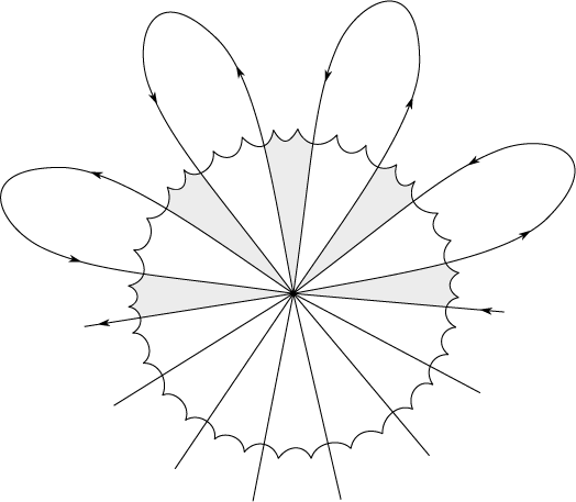
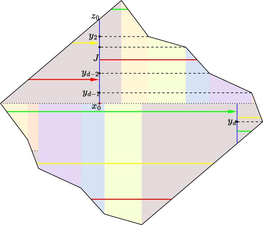

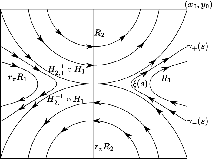


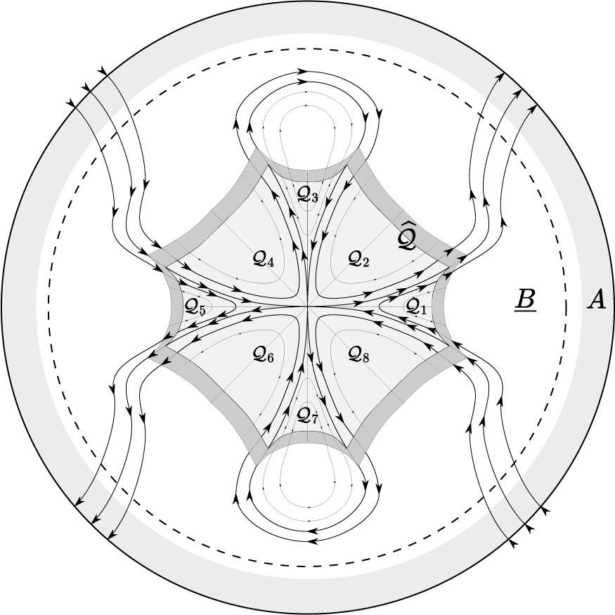
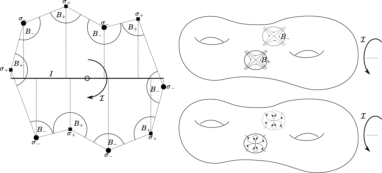
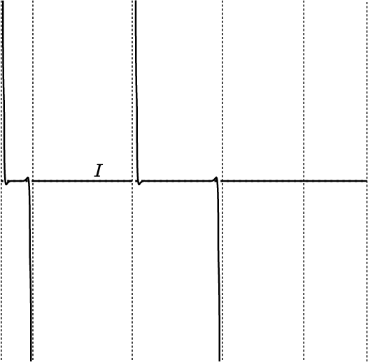


 Open access