


1. Introduction
In large eddy simulation (LES), the effect of the subgrid-scale (SGS) velocity fluctuations on the resolved flow should be modelled, and thus the aim of SGS modelling is to find the relations between the resolved flow variables and SGS stresses. A conventional approach for SGS modelling is to approximate the SGS stresses with the resolved flow variables in an arithmetic form based on turbulence theory and hypothesis. For example, an eddy viscosity model is based on the Boussinesq hypothesis that linearly relates the SGS stress tensor  $\boldsymbol {\tau }$ with the resolved strain rate tensor $\bar {\boldsymbol{\mathsf{S}}}$, i.e. $\boldsymbol {\tau }-\frac {1}{3} \text {tr}( \boldsymbol {\tau } ) {\boldsymbol{\mathsf{I}}} =-2{\nu _t} \bar {\boldsymbol{\mathsf{S}}}$, where ${\boldsymbol{\mathsf{I}}}$ is the identity tensor, and ${\nu _t}$ is an eddy viscosity to be modelled with the resolved flow variables (see, for example, Smagorinsky Reference Smagorinsky1963; Nicoud & Ducros Reference Nicoud and Ducros1999; Vreman Reference Vreman2004; Nicoud et al. Reference Nicoud, Toda, Cabrit, Bose and Lee2011; Verstappen Reference Verstappen2011; Rozema et al. Reference Rozema, Bae, Moin and Verstappen2015; Trias et al. Reference Trias, Folch, Gorobets and Oliva2015; Silvis, Remmerswaal & Verstappen Reference Silvis, Remmerswaal and Verstappen2017). Some models dynamically determine the coefficients of the eddy viscosity models (Germano et al. Reference Germano, Piomelli, Moin and Cabot1991; Lilly Reference Lilly1992; Ghosal et al. Reference Ghosal, Lund, Moin and Akselvoll1995; Piomelli & Liu Reference Piomelli and Liu1995; Meneveau, Lund & Cabot Reference Meneveau, Lund and Cabot1996; Park et al. Reference Park, Lee, Lee and Choi2006; You & Moin Reference You and Moin2007; Lee, Choi & Park Reference Lee, Choi and Park2010; Verstappen et al. Reference Verstappen, Bose, Lee, Choi and Moin2010). Other types of SGS model include the similarity model (Bardina, Ferziger & Reynolds Reference Bardina, Ferziger and Reynolds1980; Liu, Meneveau & Katz Reference Liu, Meneveau and Katz1994; Domaradzki & Saiki Reference Domaradzki and Saiki1997), the mixed model (Bardina et al. Reference Bardina, Ferziger and Reynolds1980; Zang, Street & Koseff Reference Zang, Street and Koseff1993; Liu et al. Reference Liu, Meneveau and Katz1994; Vreman, Geurts & Kuerten Reference Vreman, Geurts and Kuerten1994; Liu, Meneveau & Katz Reference Liu, Meneveau and Katz1995; Salvetti & Banerjee Reference Salvetti and Banerjee1995; Horiuti Reference Horiuti1997; Akhavan et al. Reference Akhavan, Ansari, Kang and Mangiavacchi2000), and the gradient model (Clark, Ferziger & Reynolds Reference Clark, Ferziger and Reynolds1979; Liu et al. Reference Liu, Meneveau and Katz1994). These models have been successfully applied to various turbulent flows, but there are still drawbacks to overcome. For example, the eddy viscosity model is purely dissipative, and thus the energy transfer from subgrid to resolved scales (i.e. backscatter) cannot be predicted. On the other hand, the scale similarity model (SSM) provides the backscatter but does not dissipate energy sufficiently, and thus simulations often diverge or produce inaccurate results. Therefore, an additional eddy-viscosity term is introduced and usually coupled with the SSM to properly dissipate the energy (Bardina et al. Reference Bardina, Ferziger and Reynolds1980; Liu et al. Reference Liu, Meneveau and Katz1994; Langford & Moser Reference Langford and Moser1999; Sarghini, Piomelli & Balaras Reference Sarghini, Piomelli and Balaras1999; Meneveau & Katz Reference Meneveau and Katz2000; Anderson & Domaradzki Reference Anderson and Domaradzki2012). The dynamic version of the eddy viscosity model can predict local backscatter with negative $\nu _t$, but an averaging procedure or ad hoc clipping on negative $\nu _t$ is required in actual LES to avoid numerical instability (Germano et al. Reference Germano, Piomelli, Moin and Cabot1991; Lilly Reference Lilly1992; Ghosal et al. Reference Ghosal, Lund, Moin and Akselvoll1995; Meneveau et al. Reference Meneveau, Lund and Cabot1996; Park et al. Reference Park, Lee, Lee and Choi2006; Thiry & Winckelmans Reference Thiry and Winckelmans2016).
An alternative approach for SGS modelling is to use high-fidelity direct numerical simulation (DNS) data. The optimal LES (Langford & Moser Reference Langford and Moser1999; Völker, Moser & Venugopal Reference Völker, Moser and Venugopal2002; Langford & Moser Reference Langford and Moser2004; Zandonade, Langford & Moser Reference Zandonade, Langford and Moser2004; Moser et al. Reference Moser, Malaya, Chang, Zandonade, Vedula, Bhattacharya and Haselbacher2009), based on the stochastic estimation (Adrian et al. Reference Adrian, Jones, Chung, Hassan, Nithianandan and Tung1989; Adrian Reference Adrian1990), is such an approach, where a prediction target, e.g. the SGS force (divergence of the SGS stress tensor), is expanded with input variables (velocity and velocity gradients). The coefficients of the input variables are found by minimizing the mean-squared error between the true and estimated values of the prediction target. Another example is to use a machine-learning algorithm such as the fully connected neural network (FCNN). The FCNN is a nonlinear function that maps the predefined input variables and prediction target, where the target can be the SGS stresses or SGS force. Like the optimal LES, the weight parameters of the FCNN are found by minimizing a given loss function such as the mean-squared error. In the case of two-dimensional decaying isotropic turbulence, Maulik et al. (Reference Maulik, San, Rasheed and Vedula2018) applied an FCNN-based approximate deconvolution model (Stolz & Adams Reference Stolz and Adams1999; Maulik & San Reference Maulik and San2017) to LES, where the filtered vorticity and streamfunction at multiple grid points were the inputs of FCNNs and the corresponding prediction targets were the deconvolved vorticity and streamfunction, respectively. This FCNN-based LES showed a better prediction of the kinetic energy spectrum than LES with the dynamic Smagorinsky model (DSM; see Germano et al. Reference Germano, Piomelli, Moin and Cabot1991; Lilly Reference Lilly1992). Maulik et al. (Reference Maulik, San, Rasheed and Vedula2019) used the same input together with eddy-viscosity kernels, but had the SGS force as the target. In a posteriori test, this FCNN model reasonably predicted the kinetic energy spectrum even though the prediction performance was not much better than those of the Smagorinsky and Leith models (Leith Reference Leith1968) with the model coefficients of  $C_s = 0.1\text {--}0.3$ in $\nu _t = (C_s \bar {\varDelta })^2 \vert \bar {S}\vert$, where $\bar {\varDelta }$ is the grid spacing and $\vert \bar {S}\vert = \sqrt {2 \bar {S}_{ij} \bar {S}_{ij}}$. In the case of three-dimensional forced isotropic turbulence, Vollant, Balarac & Corre (Reference Vollant, Balarac and Corre2017) used an FCNN with the target of the SGS scalar flux divergence $\boldsymbol {\nabla } \boldsymbol {\cdot } ( \overline {\boldsymbol {u} \phi }-\bar {\boldsymbol {u}}\bar {\phi })$ and the input of $\bar {\boldsymbol{\mathsf{S}}}$, where $\bar {\boldsymbol {u}}$ and $\bar {\phi }$ are the filtered velocity and passive scalar, respectively. They showed that the results from FCNN-based LES were very close to those from the filtered DNS (fDNS). Zhou et al. (Reference Zhou, He, Wang and Jin2019) reported that using the filter size as well as the velocity gradient tensor as the input variables was beneficial to predict the SGS stresses for the flow having a filter size different from that of trained data. Xie, Wang & E (Reference Xie, Wang and E2020a) used an FCNN to predict the SGS force with the input of $\nabla \bar {\boldsymbol {u}}$ at multiple grid points, and this FCNN performed better than DSM for the prediction of energy spectrum. In the case of three-dimensional decaying isotropic turbulence, Wang et al. (Reference Wang, Luo, Li, Tan and Fan2018) adopted the velocity and its first and second derivatives for the input of FCNN to predict the SGS stresses, and showed better performance in a posteriori test than that of DSM. Beck, Flad & Munz (Reference Beck, Flad and Munz2019) used a convolutional neural network (CNN) to predict the SGS force with the input of the velocity in whole domain, and showed in a priori test that the CNN-based SGS model predicted the SGS force better than an FCNN-based SGS model did. In the case of compressible isotropic turbulence, Xie et al. (Reference Xie, Li, Ma and Wang2019a) used FCNNs to predict SGS force and divergence of SGS heat flux, respectively, with the inputs of $\boldsymbol {\nabla } \tilde {\boldsymbol {u}}$, $\nabla ^2 \tilde {\boldsymbol {u}}$, $\boldsymbol {\nabla } \tilde {T}$, $\nabla ^2 \tilde {T}$, $\bar {\rho }$ and $\boldsymbol {\nabla } \bar {\rho }$ at multiple grid points, where $\rho$ is the fluid density, and $\tilde {\boldsymbol {u}}$ and $\tilde {T}$ are the mass-weighting-filtered velocity and temperature, respectively. Xie et al. (Reference Xie, Wang, Li, Wan and Chen2019b) applied FCNNs to predict the coefficients of a mixed model with the inputs of $|\tilde {\boldsymbol {\omega }}|$, $\tilde {\theta }$, $\sqrt {\tilde {\alpha }_{ij} \tilde {\alpha }_{ij}}$, $\sqrt {\tilde {S}_{ij} \tilde {S}_{ij}}$, $|\boldsymbol {\nabla } \tilde {T}|$, where $|\tilde {\boldsymbol {\omega }}|$, $\tilde {\theta }$, $\tilde {\alpha }_{ij}$ and $\tilde {S}_{ij}$ are the mass-weighting-filtered vorticity magnitude, velocity divergence, velocity gradient tensor and strain rate tensor, respectively. Xie et al. (Reference Xie, Wang, Li and Ma2019c) trained FCNNs with $\boldsymbol {\nabla } \tilde {\boldsymbol {u}}$, $\nabla ^2 \tilde {\boldsymbol {u}}$, $\boldsymbol {\nabla } \tilde {T}$ and $\nabla ^2 \tilde {T}$ at multiple grid points as the inputs to predict SGS stresses and SGS heat flux, respectively. Xie et al. (Reference Xie, Wang, Li, Wan and Chen2020b) used FCNNs to predict SGS stresses and SGS heat flux with the inputs of $\boldsymbol {\nabla } \tilde {\boldsymbol {u}}$, $\boldsymbol {\nabla } \widehat {\tilde {\boldsymbol {u}}}$, $\boldsymbol {\nabla } \tilde {T}$ and $\boldsymbol {\nabla } \hat {\tilde {T}}$ at multiple grid points, where the filter size of $\hat {\varDelta }$ is twice that of $\tilde {\varDelta }$. They (Xie et al. Reference Xie, Li, Ma and Wang2019a,Reference Xie, Wang, Li, Wan and Chenb,Reference Xie, Wang, Li and Mac, Reference Xie, Wang, Li, Wan and Chen2020b) showed that the FCNN-based LES provided more accurate kinetic energy spectrum and structure function of the velocity than those based on DSM and dynamic mixed model.
Unlike for isotropic turbulence, the progress in LES with an FCNN-based SGS model has been relatively slow for turbulent channel flow. Sarghini, de Felice & Santini (Reference Sarghini, de Felice and Santini2003) trained an FCNN with the input of filtered velocity gradient and  $\bar {u}_i^\prime \bar {u}_j^\prime$ to predict the model coefficient of the Smagorinsky model for a turbulent channel flow, where $\bar {u}_i^\prime$ is the instantaneous filtered velocity fluctuations. Pal (Reference Pal2019) trained an FCNN to predict $\nu _t$ in the eddy viscosity model with the input of filtered velocity and strain rate tensor. In Sarghini et al. (Reference Sarghini, de Felice and Santini2003) and Pal (Reference Pal2019), however, FCNNs were trained by LES data from traditional SGS models, i.e. mixed model (Bardina et al. Reference Bardina, Ferziger and Reynolds1980) and DSM, respectively, rather than by fDNS data. Wollblad & Davidson (Reference Wollblad and Davidson2008) trained an FCNN with fDNS data to predict the coefficients of the truncated proper orthogonal decomposition (POD) expansion of the SGS stresses with the input of $\bar {u}_i^\prime$, wall-normal gradient of $\bar {u} _i^\prime$, filtered pressure ( $\bar {p}$) and wall-normal and spanwise gradients of $\bar {p}$. They showed from a priori test that the predicted SGS stresses were in good agreement with those from fDNS data. However, the FCNN alone was unstable in a posteriori test, and thus the FCNN combined with the Smagorinsky model was used to conduct LES, i.e. $\tau _{ij} = c_b \tau _{ij}^{\text {FCNN}} + (1 - c_b) \tau _{ij}^{\text {Smag}}$, where $\tau _{ij}^{\text {FCNN}}$ and $\tau _{ij}^{\text {Smag}}$ were the SGS stresses from the FCNN and Smagorinsky model (with $C_s = 0.09$), respectively, and $c_b$ was a weighting parameter needed to be tuned. Gamahara & Hattori (Reference Gamahara and Hattori2017) used FCNNs to predict the SGS stresses with four input variable sets, $\{ \boldsymbol {\nabla } \bar {\boldsymbol {u}}, y \}$, $\{\boldsymbol {\nabla } \bar {\boldsymbol {u}} \}$, $\{ \bar {\boldsymbol{\mathsf{S}}},\bar {\boldsymbol{\mathsf{R}}},y \}$ and $\{\bar {\boldsymbol{\mathsf{S}}},y \}$, where $\bar {\boldsymbol{\mathsf{R}}}$ is the filtered rotation rate tensor and $y$ is the wall-normal distance from the wall. They showed in a priori test that the correlation coefficients between the true and predicted SGS stresses from $\{ \boldsymbol {\nabla } \bar {\boldsymbol {u}}, y \}$ were highest among four input sets, and even higher than those from traditional SGS models (gradient and Smagorinksy models). However, a posteriori test (i.e. actual LES) with $\{ \boldsymbol {\nabla } \bar {\boldsymbol {u}}, y \}$ did not provide any advantage over the LES with the Smagorinsky model. This kind of the inconsistency between a priori and a posteriori tests had been also observed during the development of traditional SGS models (Liu et al. Reference Liu, Meneveau and Katz1994; Vreman, Geurts & Kuerten Reference Vreman, Geurts and Kuerten1997; Park, Yoo & Choi Reference Park, Yoo and Choi2005; Anderson & Domaradzki Reference Anderson and Domaradzki2012).
Previous studies (Wollblad & Davidson Reference Wollblad and Davidson2008; Gamahara & Hattori Reference Gamahara and Hattori2017) showed that FCNN is a promising tool for modelling SGS stresses from a priori test, but it is unclear why FCNN-based LESs did not perform better for a turbulent channel flow than LESs with traditional SGS models. Thus, a more systematic investigation on the SGS variables such as the SGS dissipation and transport is required to diagnose the performance of FCNN. The input variables for the FCNN should be also chosen carefully based on the characteristics of the SGS stresses. Therefore, the objective of the present study is to develop an FCNN-based SGS model for a turbulent channel flow, based on both a priori and a posteriori tests, and to find appropriate input variables for the successful LES with FCNN. We train FCNNs with different input variables such as  $\bar {\boldsymbol{\mathsf{S}}}$ and $\boldsymbol {\nabla } \bar {\boldsymbol {u}}$, and the target to predict is the SGS stress tensor. We also test $\bar {\boldsymbol {u}}$ and $\partial \bar {\boldsymbol {u}} / \partial y$ as the input for FCNN (note that these were the input variables of the optimal LES for a turbulent channel flow by Völker et al. Reference Völker, Moser and Venugopal2002). The input and target data are obtained by filtering the data from DNS of a turbulent channel flow at the bulk Reynolds number of $Re_b =5600$ ( $Re_\tau = u_\tau \delta / \nu = 178$), where $u_\tau$ is the wall-shear velocity, $\delta$ is the channel half height and $\nu$ is the kinematic viscosity. In a priori test, we examine the variations of the predicted SGS dissipation, backscatter and SGS transport with the input variables, which are known to be important variables for successful LES of a turbulent channel flow (Piomelli, Yu & Adrian Reference Piomelli, Yu and Adrian1996; Völker et al. Reference Völker, Moser and Venugopal2002; Park et al. Reference Park, Lee, Lee and Choi2006). In a posteriori test, we perform LESs with FCNN-based SGS models at $Re_\tau = 178$ and estimate their prediction performance by comparing the results with those from the fDNS data and LESs with DSM and SSM (Liu et al. Reference Liu, Meneveau and Katz1994). The details about DNS and FCNN are given in § 2. The results from a priori and a posteriori tests at $Re_\tau = 178$ are given in § 3. Applications of the FCNN trained at $Re_\tau = 178$ to LES of a higher-Reynolds-number flow ( $Re_\tau = 723$) and to LES with a different grid resolution at $Re_\tau = 178$ are also discussed in § 3, followed by conclusions in § 4.
2. Numerical details
2.1. NN-based SGS model
The governing equations for LES are the spatially filtered continuity and Navier–Stokes equations,
 \begin{gather} \frac{\partial {\bar{u}_i}}{\partial {x_i}}=0, \end{gather}
 \begin{gather}\frac{\partial {\bar{u}_i}}{\partial t}+\frac{\partial \bar{u}_i \bar{u}_j}{\partial x_j}=-\frac{\partial \bar{p}}{\partial x_i}+\frac{1}{Re}\frac{{{\partial }^2}\bar{u}_i}{\partial x_j\partial x_j}-\frac{\partial \tau_{ij}}{\partial x_j}, \end{gather}
where  $x_1~({=}x)$, $x_2~({=}y)$ and $x_3~({=}z)$ are the streamwise, wall-normal and spanwise directions, respectively, $u_i\ ({=}u, v, w)$ are the corresponding velocity components, $p$ is the pressure, $t$ is time, the overbar denotes the filtering operation and $\tau _{ij}\ ({=}\overline {u_i u_j}-\bar {u}_i\bar {u}_j)$ is the SGS stress tensor. We use a FCNN (denoted as NN hereafter) with the input of the filtered flow variables to predict $\tau _{ij}$. The database for training the NN is obtained by filtering the instantaneous flow fields from DNS of a turbulent channel flow at $Re_\tau = 178$ (see § 2.2). To estimate the performance of the present NN-based SGS model, we perform two additional LESs with the DSM (Germano et al. Reference Germano, Piomelli, Moin and Cabot1991; Lilly Reference Lilly1992) and SSM (Liu et al. Reference Liu, Meneveau and Katz1994). For the DSM, $\tau _{ij}-\frac {1}{3}\tau _{kk}\delta _{ij}= -2 C^2 | \bar {S} |\bar {S}_{ij}$, where $C^2=-\frac {1}{2} \langle L_{ij}M_{ij} \rangle _h / \langle M_{ij}M_{ij} \rangle _h$, $| \bar {S}|=\sqrt {2\bar {S}_{ij}\bar {S}_{ij}}, \bar {S}_{ij} = \frac {1}{2} (\partial \bar {u}_i/\partial x_j + \partial \bar {u}_j/\partial x_i ), L_{ij}=\widetilde {\bar {u}_i \bar {u}_j}-{\tilde {\bar {u}}}_i {{\tilde {\bar {u}}}_j}, M_{ij}$ $={( \tilde {\varDelta }/\bar {\varDelta } )}^2 | \tilde {\bar {S}} | {\tilde {\bar {S}}}_{ij} \!-\! {\widetilde {| \bar {S} |\bar {S}_{ij}}}$, $\bar {\varDelta }$ and $\tilde {\varDelta }\ ({=}2\bar {\varDelta })$ denote the grid and test filter sizes, respectively, and $\langle \rangle _h$ denotes averaging in the homogeneous ( $x$ and $z$) directions. For the SSM, $\tau _{ij}=\widetilde {\bar {u}_i\bar {u}_j}-{\tilde {\bar {u}}}_i{{\tilde {\bar {u}}}_j}$, where $\tilde {k}_{cut}=0.5{\bar {k}_{cut}}$ and $k_{cut}$ is the cut-off wavenumber.
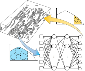
The NN adopted in the present study has two hidden layers with 128 neurons per hidden layer, and the output of the NN is the six components of  $\tau _{ij}$ (figure 1). Previous studies used one (Gamahara & Hattori Reference Gamahara and Hattori2017; Maulik & San Reference Maulik and San2017; Maulik et al. Reference Maulik, San, Rasheed and Vedula2018; Zhou et al. Reference Zhou, He, Wang and Jin2019) or two (Sarghini et al. Reference Sarghini, de Felice and Santini2003; Wollblad & Davidson Reference Wollblad and Davidson2008; Vollant et al. Reference Vollant, Balarac and Corre2017; Wang et al. Reference Wang, Luo, Li, Tan and Fan2018; Maulik et al. Reference Maulik, San, Rasheed and Vedula2019; Xie et al. Reference Xie, Li, Ma and Wang2019a,Reference Xie, Wang, Li, Wan and Chenb,Reference Xie, Wang, Li and Mac, Reference Xie, Wang and E2020a,Reference Xie, Wang, Li, Wan and Chenb) hidden layers, and Gamahara & Hattori (Reference Gamahara and Hattori2017) showed that 100 neurons per hidden layer were sufficient for the accurate predictions of $\tau _{ij}$ for a turbulent channel flow in a priori test. We also tested NN with three hidden layers, but more hidden layers than two did not further improve the performance both in a priori and a posteriori tests (see the Appendix).
Schematic diagram of the present NN with two hidden layers (128 neurons per hidden layer). Here,  $\boldsymbol {q}\ ({=}[q_1, q_2,\ldots , q_{N_q}]^\textrm {T})$ is the input of NN, $N_q$ is the number of input components (see table 1) and $\boldsymbol {s}\ ({=}[s_1,s_2,\ldots ,s_6]^\textrm {T})$ is the output of NN.

In the present NN, the output of the  $m$th layer, $\boldsymbol {h}^{(m)}$, is as follows:
 \begin{align} \left.\begin{aligned} h_i^{(1)} &= q_i \ (i=1,2,\ldots,N_q);\\ h_j^{(2)} &= \max[0, r_j^{(2)}], r_j^{(2)}\\ &= \gamma_j^{(2)} \left.\left ( \sum_{i=1}^{N_q}{W_{ij}^{(1)(2)} h_i^{(1)}} +b_j^{(2)}-\mu_j^{(2)} \right )\right/\sigma_j^{(2)}+\beta_j^{(2)} \ (\,j=1,2,\ldots,128); \\ h_k^{(3)} &= \max [0, r_k^{(3)}], r_k^{(3)}\\ &= \gamma_k^{(3)} \left.\left ( \sum_{j=1}^{128}{W_{jk}^{(2)(3)} h_j^{(2)}} +b_k^{(3)}-\mu_k^{(3)}\right )\right/\sigma_k^{(3)}+ \beta_k^{(3)} \ (k=1,2,\ldots,128); \\ h_l^{(4)} &= s_l = \sum\limits_{k=1}^{128}{W_{kl}^{(3)(4)} h_k^{(3)}} + b_l^{(4)} \ (l=1,2,\ldots,6),\end{aligned}\right\} \end{align}
where  $q_i$ is the input, $N_q$ is the number of input components, $\boldsymbol{\mathsf{W}}^{(m)(m+1)}$ is the weight matrix between the $m$th and $(m+1)$th layers, $\boldsymbol {b}^{(m)}$ is the bias of the $m$th layer, $s_l$ is the output and $\boldsymbol {\mu }^{(m)}$, $\boldsymbol {\sigma }^{(m)}$, $\boldsymbol {\gamma }^{(m)}$ and $\boldsymbol {\beta }^{(m)}$ are parameters for a batch normalization (Ioffe & Szegedy Reference Ioffe and Szegedy2015). We use a rectified linear unit (ReLU; see Nair & Hinton Reference Nair and Hinton2010), $\boldsymbol {h}^{(m)} = \max [0, \boldsymbol {r}^{(m)}]$, as the activation function at the hidden layers. We also tested other typical activation functions such as sigmoid and hyperbolic tangent functions, but the convergence of the loss function (2.4) was faster with the ReLU than with others. Here $\boldsymbol{\mathsf{W}}^{(m)(m+1)}$, $\boldsymbol {b}^{(m)}$, $\boldsymbol {\gamma }^{(m)}$ and $\boldsymbol {\beta }^{(m)}$ are trainable parameters that are optimized to minimize the loss function defined as
 \begin{equation} L=\frac{1}{2N_b}\frac{1}{6}\sum_{l=1}^{6}{\sum_{n=1}^{N_b}{{\left( s_{l,n}^{\text{fDNS}}-s_{l,n} \right)}^2}} + 0.005\sum_{o}{w_o^2}, \end{equation}
where  $s_{l,n}^{\text {fDNS}}$ is the SGS stresses obtained from fDNS data, $N_b$ is the number of minibatch data (128 in this study following Kingma & Ba Reference Kingma and Ba2014) and $w_o$ denotes the components of $\boldsymbol{\mathsf{W}}^{(m)(m+1)}$. An adaptive moment estimation (Kingma & Ba Reference Kingma and Ba2014), which is a variant of gradient descent method, is applied to update the trainable parameters and the gradients of the loss function with respect to those parameters are calculated through the chain rule of derivatives (Rumelhart, Hinton & Williams Reference Rumelhart, Hinton and Williams1986; LeCun, Bengio & Hinton Reference LeCun, Bengio and Hinton2015). All training procedures are conducted using the Python open-source library TensorFlow.
We choose five different input variables (corresponding to NN1–NN5), as listed in table 1. Six components of  $\bar {S}_{ij}$ and nine components of $\bar {\alpha }_{ij}\ ({=}\partial {\bar {u}_i}/\partial {x_j})$ at each grid point are the inputs to NN1 and NN2, respectively, and the output is six components of $\tau _{ij}$ at the same grid location. The input $\bar {\alpha }_{ij}$ is selected for NN2 because $\tau _{ij}$ can be written as $\tau _{ij} = 2\gamma \bar {\alpha }_{ik}\bar {\alpha }_{jk}+O(\gamma ^2)$, where $\gamma ( \zeta )=\int _{-\infty }^{\infty }{\xi ^2 G( \xi ,\zeta )}\,\text {d}\xi$ and $G( \xi ,\zeta )$ is the kernel of the filter (Bedford & Yeo Reference Bedford and Yeo1993). On the other hand, a general class of SGS model based on the local velocity gradient (Lund & Novikov Reference Lund and Novikov1992; Silvis et al. Reference Silvis, Bae, Trias, Abkar and Verstappen2019) can be expressed as $\tau _{ij}=\sum \nolimits _{k=0}^5{{c^{(k)}}T_{ij}^{(k)}}$, where $c^{(k)}$ is the model coefficient, $T_{ij}^{(0)}=\delta _{ij}$, $T_{ij}^{(1)}=\bar {S} _{ij}$, $T_{ij}^{(2)}=\bar {S}_{ik} \bar {S}_{kj}$, $T_{ij}^{(3)}=\bar {R}_{ik} \bar {R}_{kj}$, $T_{ij}^{(4)}=\bar {S}_{ik} \bar {R}_{kj} - \bar {R}_{ik} \bar {S}_{kj}$, $T_{ij}^{(5)}=\bar {S}_{ik} \bar {S}_{kl} \bar {R}_{lj} - \bar {R}_{ik} \bar {S}_{kl} \bar {S}_{lj}$ and $\bar {R}_{ij}$ is the filtered rotation rate tensor. Thus, NN1 can be regarded as an SGS model including $T_{ij}^{(0)}$, $T_{ij}^{(1)}$ and $T_{ij}^{(2)}$, but it directly predicts $\tau _{ij}$ through a nonlinear process of NN rather than predicting $c^{(k)}$. In NN3 and NN4, a stencil of data at $3(x)\times 3(z)$ grid points are the input, and $\tau _{ij}$ at the center of this stencil is the output. In NN5, the filtered velocity and wall-normal velocity gradient at $3(x)\times 3(z)$ grid points are the input variables, and the output is the same as that of NN3 and NN4. The use of a stencil of data for NN3–NN5 is motivated by the results of Xie et al. (Reference Xie, Wang, Li and Ma2019c) that using a stencil of input variables ( $\bar {\alpha }_{ij}$ and temperature gradient) predicted $\tau _{ij}$ better than using the same input only at one grid point. The choice of $\bar {u}_i$ and $\partial \bar {u}_i/\partial y$ as the input of NN5 is also motivated by the results of optimal LES by Völker et al. (Reference Völker, Moser and Venugopal2002), in which LES with the input of both $\bar {u}_i$ and $\partial \bar {u}_i/\partial y$ outperformed that with the input of $\bar {u}_i$ alone. We also considered an NN with the input of $\bar {u}_i$ at $n_x(x) \times 3(y) \times n_z(z)$ grid points, where $n_x = n_z = 3$, 5, 7, or 9. The results with these three-dimensional multiple input grid points were little different in a priori tests from that of NN5. As shown in § 3, the results with NN3–NN5 in a priori tests are better than those with NN1 and NN2 (single input grid point), but actual LES (i.e. a posteriori test) with NN3–NN5 are unstable. Therefore, we did not seek to adopt more input grid points. Note also that we train a single NN for all $y$ locations using pairs of the input and output variables. The relations between these variables are different for different $y$ locations, and thus $y$ locations are implicitly embedded in this single NN. One may train an NN at each $y$ location, but this procedure increases the number of NNs and the memory size. On the other hand, Gamahara & Hattori (Reference Gamahara and Hattori2017) provided $y$ locations as an additional input variable for a single NN, but found that the result of a priori test with $y$ location was only slightly better than that without $y$ location. Therefore, we do not attempt to include $y$ location as an additional input variable in this study.
Input variables of NN models.

While training NN1–NN5, the input and output variables are normalized in wall units, which provides successful results because the flow variables in turbulent channel flow are well scaled in wall units (see § 3). As the performance of an NN depends on the normalization of input and output variables (see, for example, Passalis et al. Reference Passalis, Tefas, Kanniainen, Gabbouj and Iosifidis2019), we considered two more normalizations: one was with the centreline velocity ( $U_c$) and channel half height ( $\delta$), and the other was such that the input and output variables were scaled to have zero mean and unit variance at each $y$ location, e.g. $\tau _{ij}^*(x,y,z,t)= (\tau _{ij}(x,y,z,t)-\tau _{ij}^{mean}(y) )/\tau _{ij}^{rms}(y)$ (no summation on $i$ and $j$), where the superscripts mean and rms denote the mean and root-mean-square (r.m.s.) values, respectively. The first normalization was not successful for the prediction of a higher-Reynolds-number flow with an NN trained at lower Reynolds number, because the near-wall flow was not properly scaled with this normalization. The second normalization requires a priori knowledge on $\tau _{ij}^{mean}(y)$ and $\tau _{ij}^{rms}(y)$ even for a higher-Reynolds-number flow to predict. Thus, we did not take the second normalization either.
Figure 2 shows the variations of the training error  $\epsilon _\tau$ with the epoch, and the correlation coefficients $\rho _\tau$ between true and predicted SGS stresses for NN1–NN5, where $\epsilon _\tau$ and $\rho _\tau$ are defined as
 \begin{gather} \epsilon_\tau=\frac{1}{2{N}_{data}}\frac{1}{6}\sum_{l=1}^{6}{\sum_{n=1}^{{N}_{data}}{{\left( s_{l,n}^{\text{fDNS}}-s_{l,n} \right)}^2}}, \end{gather}
 \begin{gather}\rho_\tau = \left.\sum_{l=1}^6 \sum_{n=1}^{{{{N}}_{{data}}}}\left( s_{l,n}^{\text{fDNS}} s_{l,n} \right)\right/\left( \sqrt{ \sum_{l=1}^6 \sum_{n=1}^{{{N}_{data}}}{\left( s_{l,n}^{\text{fDNS}} \right)^2}}\sqrt{\sum_{l=1}^6 \sum_{n=1}^{{{N}_{data}}}{\left( s_{l,n} \right)^2}} \right). \end{gather}
Here, one epoch denotes one sweep through the entire training dataset (Hastie, Tibshirani & Friedman Reference Hastie, Tibshirani and Friedman2009), and  ${N}_{data}$ is the number of entire training data. The training errors nearly converge at 20 epochs (figure 2a). In terms of computational time using a single graphic process unit (NVIDIA GeForce GTX 1060), about 1 min is spent for each epoch. The correlation coefficients from the training and test datasets are quite similar to each other (figure 2b), indicating that severe overfitting is not observed for NN1–NN5. The training error and correlation coefficient are smaller and larger, respectively, for NN3–NN5 than those for NN1 and NN2.
Training error and correlation coefficient by NN1–NN5: ( $a$) training error versus epoch; ( $b$) correlation coefficient. In ( $a$), red solid line, NN1; blue solid line, NN2; red dashed line, NN3; blue dashed line, NN4; green solid line, NN5. In ( $b$), gray and black bars are the correlation coefficients for training and test datasets, respectively, where the number of test data is the same as that of the training data ( ${N}_{data} = 1\,241\,600$ (§ 2.2)).

Sarghini et al. (Reference Sarghini, de Felice and Santini2003) and Pal (Reference Pal2019) indicated that required computational time for their LESs with NNs was less than that with traditional SGS models. When an NN is used for obtaining the SGS stresses, its cost depends on the numbers of hidden layers and neurons therein as well as the choices of input and output variables. Actually, in the present study, the computational time required for one computational time-step advancement with NN1 is approximately 1.3 times that with a traditional SGS model such as DSM.
2.2. Details of DNS and input and output variables
A DNS of turbulent channel flow at  $Re_b = 5600\ (Re_\tau = 178)$ is conducted to obtain the input and output of NN1–NN5 (table 1), where $Re_b$ is the bulk Reynolds number defined by $Re_b = U_b (2 \delta ) / \nu$, $U_b$ is the bulk velocity and $Re_\tau = u_\tau \delta / \nu$ is the friction Reynolds number. The Navier–Stokes and continuity equations are solved in the form of the wall-normal vorticity and the Laplacian of the wall-normal velocity, as described in Kim, Moin & Moser (Reference Kim, Moin and Moser1987). The dealiased Fourier and Chebyshev polynomial expansions are used in the homogeneous ( $x$ and $z$) and wall-normal ( $y$) directions, respectively. A semi-implicit fractional step method is used for time integration, where a third-order Runge–Kutta and second-order Crank–Nicolson methods are applied to the convection and diffusion terms, respectively. A constant mass flux in a channel is maintained by adjusting the mean pressure gradient in the streamwise direction at each time step.
Table 2 lists the computational parameters of DNS, where  $N_{x_i}$ are the numbers of grid points in $x_i$ directions, $L_{x_i}$ are the corresponding computational domain sizes, $\Delta x$ and $\Delta z$ are the uniform grid spacings in $x$ and $z$ directions, respectively, and $\Delta y^+_{min}$ is the smallest grid spacing at the wall in the wall-normal direction. Here $\varDelta _x$ and $\varDelta _z$ are the filter sizes in $x$ and $z$ directions, respectively, and they are used for obtaining fDNS data. We apply the spectral cut-off filter only in the wall-parallel ( $x$ and $z$) directions as in the previous studies (Piomelli et al. Reference Piomelli, Cabot, Moin and Lee1991, Reference Piomelli, Yu and Adrian1996; Völker et al. Reference Völker, Moser and Venugopal2002; Park et al. Reference Park, Lee, Lee and Choi2006). The use of only wall-parallel filters can be justified because small scales are efficiently filtered out by wall-parallel filters and wall-normal filtering through the truncation of the Chebyshev mode violates the continuity unless the divergence-free projection is performed (Völker et al. Reference Völker, Moser and Venugopal2002; Park et al. Reference Park, Lee, Lee and Choi2006). The Fourier coefficient of a filtered flow variable $\hat {\bar {f}}$ is defined as
 \begin{equation} \hat{\bar{f}}\left( k_x,y,k_z,t \right)= \hat{f}\left( k_x,y,k_z,t \right) H\left( k_{x,cut}-\left| k_x \right| \right)H\left( k_{z,cut}-\left| k_z \right| \right), \end{equation}
where  $\hat {f}$ is the Fourier coefficient of an unfiltered flow variable $f$,
$f$,  $H$ is the Heaviside step function and $k_{x,cut}$ and $k_{z,cut}$ are the cut-off wavenumbers in $x$ and $z$ directions, respectively. The filter sizes in table 2, $\varDelta _x^+$ and $\varDelta _z^+$, are the same as those in Park et al. (Reference Park, Lee, Lee and Choi2006), and the corresponding cut-off wavenumbers are $k_{x,cut} = 8\ (2{\rm \pi} /L_x)$ and $k_{z,cut} = 8\ (2{\rm \pi} /L_z)$, respectively. We use the input and output database at $Re_{\tau }=178$ to train NN1–NN5. The training data are collected at every other grid point in $x$ and $z$ directions to exclude highly correlated data, and at all grid points in $y$ direction from 200 instantaneous fDNS fields. Then, the number of training data from 200 fDNS fields is 1 241 600 ( ${=}200\times N_x^{\text {fDNS}}/2 \times N_z^{\text {fDNS}}/2 \times N_y$), where $N_x^{\text {fDNS}}=L_x k_{x,cut}/{\rm \pi}$ and $N_z^{\text {fDNS}}=L_z k_{z,cut}/{\rm \pi}$. We have also tested 300 fDNS fields for training NNs, but their prediction performance for the SGS stresses is not further improved, so the number of training data used is sufficient for the present NNs. A DNS at a higher Reynolds number of $Re_\tau = 723$ is also carried out, and its database is used to estimate the prediction capability of the present NN-based SGS model for untrained higher-Reynolds-number flow.
Computational parameters of DNS. Here, the superscript  $+$ denotes the wall unit and $\Delta T$ is the sampling time interval of the instantaneous DNS flow fields for constructing the input and output database.

3. Results
In § 3.1, we perform a priori tests for two different Reynolds numbers,  $Re_\tau = 178$ and $723$, in which the SGS stresses are predicted by NN1–NN5 with the input variables from fDNS at each Reynolds number, and compared with the SGS stresses from fDNS. Note that NN1–NN5 are constructed at $Re_\tau = 178$ and $Re_\tau = 723$ is an untrained higher Reynolds number. The filter sizes used in a priori tests, $\varDelta _x^+$ and $\varDelta _z^+$, are given in table 2. In § 3.2, a posteriori tests (i.e. actual LESs solving (2.1) and (2.2)) with NN1–NN5 are performed for a turbulent channel flow at $Re_\tau = 178$ and their results are compared with those of fDNS. Furthermore, LES with NN1 (trained at $Re_\tau = 178$) is carried out for a turbulent channel flow at $Re_\tau = 723$ and its results are compared with those of fDNS. Finally, in § 3.3, we provide the results when the grid resolution in LES is different from that used in training NN1, and suggest a way to obtain good results.
3.1. A priori test
Figure 3 shows the mean SGS shear stress  $\langle \tau _{xy} \rangle$ and dissipation $\langle \varepsilon _{SGS} \rangle$ predicted by NN1–NN5, together with those of fDNS and from DSM and SSM, where $\varepsilon _{SGS}= - \tau _{ij} \bar {S}_{ij}$ and $\langle \,\rangle$ denotes the averaging in the homogeneous directions and time. Predictions of $\langle \tau _{xy} \rangle$ by NNs (except that by NN2) are better than those by DSM and SSM, and NN5 provides an excellent prediction of $\langle \varepsilon _{SGS} \rangle$ albeit other NN models are also good in the estimation of $\langle \varepsilon _{SGS} \rangle$. Table 3 lists the correlation coefficients $\rho$ between the true and predicted $\tau _{xy}$ and $\varepsilon _{SGS}$, respectively. The values of $\tau _{xy}$ predicted by DSM and SSM have very low correlations with true $\tau _{xy}$, as reported by Liu et al. (Reference Liu, Meneveau and Katz1994) and Park et al. (Reference Park, Yoo and Choi2005). On the other hand, NN1–NN5 have much higher correlations of $\tau _{xy}$ and $\varepsilon _{SGS}$ than those by DSM and SSM, indicating that instantaneous $\tau _{xy}$ and $\varepsilon _{SGS}$ are relatively well captured by NN1–NN5. These SGS variables are even better predicted by having the input variables at multiple grid points (NN3–NN5) than at single grid point (NN1 and NN2). As we show in the following, however, high correlation coefficients of $\tau _{xy}$ and $\varepsilon _{SGS}$ in a priori test do not necessarily guarantee excellent prediction performance in actual LES.
Mean SGS shear stress and dissipation predicted by NN1–NN5 (a priori test at  $Re_\tau =178$): ( $a$) mean SGS shear stress $\langle \tau _{xy} \rangle$; ( $b$) mean SGS dissipation $\langle \varepsilon _{SGS} \rangle$. ${\bullet }$, fDNS; red solid line, NN1; blue solid line, NN2; red dashed line, NN3; blue dashed line, NN4; green solid line, NN5; $+$, DSM; $\triangledown$, SSM.

Correlation coefficients between the true and predicted  $\tau _{xy}$ and $\varepsilon _{SGS}$.

Figure 4(a) shows the mean SGS transport  $\langle T_{SGS} \rangle$, where $T_{SGS}=\partial (\tau _{ij} \bar {u}_i) / \partial x_j$. Völker et al. (Reference Völker, Moser and Venugopal2002) indicated that a good prediction of $\langle T_{SGS} \rangle$ is necessary for an accurate LES, and the optimal LES provided good representation of $\langle T_{SGS} \rangle$ in a posteriori test. Among NN models considered, NN5 shows the best agreement of $\langle T_{SGS} \rangle$ with that of fDNS, but NN1 and NN2 are not good at accurately predicting $\langle T_{SGS} \rangle$ although they are still better than SSM. Figure 4(b) shows the mean backward SGS dissipation (backscatter, i.e. energy transfer from subgrid to resolved scales), $\langle \varepsilon _{SGS}^- \rangle = \frac {1}{2} \langle \varepsilon _{SGS}-| \varepsilon _{SGS} | \rangle$. $\langle \varepsilon _{SGS}^- \rangle = 0$ for DSM owing to the averaging procedure in determining the model coefficient. The mean backscatters from SSM and NN3–NN5 show reasonable agreements with that of fDNS, but NN1 and NN2 severely underpredict the backscatter. An accurate prediction of backscatter is important in wall-bounded flows, because it is related to the bursting and sweep events (Härtel et al. Reference Härtel, Kleiser, Unger and Friedrich1994; Piomelli et al. Reference Piomelli, Yu and Adrian1996). However, SGS models with non-negligible backscatter such as SSM do not properly dissipate energy and incur numerical instability in actual LES (Liu et al. Reference Liu, Meneveau and Katz1994; Akhavan et al. Reference Akhavan, Ansari, Kang and Mangiavacchi2000; Meneveau & Katz Reference Meneveau and Katz2000; Anderson & Domaradzki Reference Anderson and Domaradzki2012). For this reason, some NN-based SGS models suggested in the previous studies clipped the backscatter to be zero for ensuring stable LES results (Maulik et al. Reference Maulik, San, Rasheed and Vedula2018, Reference Maulik, San, Rasheed and Vedula2019; Zhou et al. Reference Zhou, He, Wang and Jin2019). Therefore, the accuracy and stability in the solution from LES with NN3–NN5 may not be guaranteed, even if these models properly predict the backscatter and produce high correlation coefficients between the true and predicted SGS stresses.
Mean SGS transport and backward SGS dissipation predicted by NN1–NN5 (a priori test at  $Re_\tau =178$): ( $a$) mean SGS transport $\langle T_{SGS} \rangle$; ( $b$) mean backward SGS dissipation (backscatter) $\langle \varepsilon _{SGS}^{-} \rangle$. ${\bullet }$, fDNS; red solid line, NN1; blue solid line, NN2; red dashed line, NN3; blue dashed line, NN4; green solid line, NN5; $+$, DSM; $\triangledown$, SSM.

Figure 5 shows the statistics from a priori test for  $Re_\tau = 723$ with NN-based SGS models trained at $Re_\tau = 178$. The statistics predicted by NN1–NN5 for $Re_\tau = 723$ show very similar behaviours to those for $Re_\tau = 178$, except for an underprediction of $\langle \tau _{xy} \rangle$ by NN1 (similar to that by DSM) which does not degrade its prediction capability in a posteriori test (see § 3.2).
Statistics from a priori test at  $Re_\tau =723$: ( $a$) mean SGS shear stress $\langle \tau _{xy} \rangle$; ( $b$) mean SGS dissipation $\langle \varepsilon _{SGS} \rangle$; ( $c$) mean SGS transport $\langle T_{SGS} \rangle$; ( $d$) mean backscatter $\langle \varepsilon _{SGS}^{-} \rangle$. ${\bullet }$, fDNS; red solid line, NN1; blue solid line, NN2; red dashed line, NN3; blue dashed line, NN4; green solid line, NN5; $+$, DSM; $\triangledown$, SSM. Here, NN1–NN5 are trained with fDNS at $Re_\tau =178$.

3.2. A posteriori test
In this section, a posteriori tests (i.e. actual LESs) with NN-based SGS models are conducted for a turbulent channel flow with a constant mass flow rate ( $Re_b = 5600$ or 27 600). Numerical methods for solving the filtered Navier–Stokes and continuity equations are the same as those of DNS described in § 2.2. Table 4 shows the computational parameters of LES. The grid resolution for the cases of LES178 is the same as that of Park et al. (Reference Park, Lee, Lee and Choi2006). The cases of LES178 have nearly the same grid resolutions in wall units (because of slightly different values of $Re_\tau$) in $x$ and $z$ directions as those of fDNS used in training NNs, and the cases of LES178c and LES178f use larger and smaller grid sizes in $x$ and $z$ directions than those of trained data, respectively. In the case of LES723 ( $Re_\tau = 723$), the grid sizes in wall units in $x$ and $z$ directions are nearly the same as those of trained data.
Computational parameters of LES. Here, the computations are performed at constant mass flow rates (i.e.  $Re_b = 5600$ and 27 600) and $Re_\tau$ given in this table are the results of LESs. For $Re_b = 5600$ and 27 600, the domain sizes in $x$ and $z$ directions are $2 {\rm \pi}\delta \times {\rm \pi}\delta$ and ${\rm \pi} \delta \times 0.5{\rm \pi} \delta$, respectively. $\Delta y^+_{min} = 0.4$ for all simulations, and $\Delta y^+_{min}$, $\Delta x^+$ and $\Delta z^+$ in this table are computed with $u_\tau$ from DNS (table 2).

In the present LESs with NN3–NN5 and SSM, we clip the SGS stresses to be zero wherever backscatter occurs, i.e.  $\tau _{ij}=0$ when $\varepsilon _{SGS}<0$, as done in the previous studies (Maulik et al. Reference Maulik, San, Rasheed and Vedula2018, Reference Maulik, San, Rasheed and Vedula2019; Zhou et al. Reference Zhou, He, Wang and Jin2019). Otherwise, the solution diverges. While removing the backscatter, we rescale the SGS stresses to maintain the net amount of SGS dissipation in the computational domain $V$ as follows:
 \begin{equation} \tau_{ij}^\ast = \frac{1}{2} \left[ 1 + \text{sign} (\varepsilon_{SGS}) \right] \tau_{ij} \cdot \frac{\displaystyle\int_V \varepsilon_{SGS}\, \text{d}V} {\tfrac{1}{2} \displaystyle\int_V \left( \varepsilon_{SGS} + \vert \varepsilon_{SGS} \vert \right ) \, \text{d}V}. \end{equation}
This backscatter clipping and rescaling on  $\tau _{ij}$ is similar to that of Akhavan et al. (Reference Akhavan, Ansari, Kang and Mangiavacchi2000) in their development of dynamic two-component model. For the cases of LESs with NN1 and NN2, we obtain stable solutions without any special treatment such as the clipping, wall damping or averaging over homogeneous directions and, thus, we perform LESs with and without clipping, respectively. In LES with DSM, an averaging procedure is included to determine the model coefficient, as mostly done in previous studies. As the present simulations are conducted for a constant mass flow rate in a channel, the wall-shear velocity or $Re_\tau$ changes depending on the choice of SGS models. Those $Re_\tau$ are listed in table 4. For $Re_b = 5600$, $Re_\tau$ from LES178 are well predicted by NN1 and NN2 even without clipping (less than 2 % error) and by NN3–NN5 with clipping (less than 3 % error). On the other hand, $Re_\tau$ from no SGS model has about 10 % error.
Figure 6 shows the mean velocity profiles from LES178 for various SGS models without and with clipping the backscatter, respectively. Without clipping, LESs with NN1 and NN2 show excellent predictions of the mean velocity, but those with NN3–NN5 and SSM diverge. On the other hand, with clipping, LESs with all the SGS models considered provide very good predictions of the mean velocity, which clearly indicates that backscatter incurs numerical instability in LES. Therefore, in the following, we present the results of LESs with clipping for NN3–NN5, and without clipping for NN1 and NN2, respectively.
Mean velocity profiles from LES178 (a posteriori test): ( $a$) without clipping the backscatter; ( $b$) with clipping the backscatter. ${\bullet }$, fDNS; red solid line, NN1; blue solid line, NN2; red dashed line, NN3; blue dashed line, NN4; green solid line, NN5; $+$, DSM; $\triangledown$, SSM; $\circ$, no SGS model. LESs with NN3–NN5 and SSM without clipping diverged.

Figure 7 shows the statistics of various turbulence quantities from LES178 with NN1–NN5, together with those of fDNS and from LESs with DSM and SSM. All NNs considered show good predictions of the r.m.s. velocity fluctuations (figure 7a). While LES without the SGS model (i.e. coarse DNS) fortuitously well predicts  $\bar {u}_{rms}$ owing to overpredicted friction velocity, LES with DSM overpredicts it (Park et al. Reference Park, Lee, Lee and Choi2006). As DSM determines the model coefficient $C^2 (y)$ to be uniform in the homogeneous directions ignoring the locality of $C^2 (x,y,z)$, its prediction performance of local SGS dissipation is degraded and may result in the overprediction of $\bar {u}_{rms}$. For the predictions of the Reynolds shear stress and SGS shear stress, NN1 performs the best among all the SGS models considered (figures 7 $b$ and 7 $c$). On the other hand, NN2 underpredicts the Reynolds shear stress and significantly overpredicts the SGS shear stress. This result is consistent with that of a priori test (figure 3a). The overprediction of $\langle \tau _{xy} \rangle$ results in the underprediction of $- \langle \bar {u}^\prime \bar {v}^\prime \rangle$ from the total shear stress equation, $\textrm {d} \langle \bar {u}^+ \rangle / {\textrm {d} y}^+ - \langle \bar {u}^\prime \bar {v}^\prime \rangle / u_\tau ^2 - \langle \tau _{xy} \rangle / u_\tau ^2 = 1 - y / \delta$. NN3–NN5 slightly overpredict the Reynolds shear stress but underpredict the SGS shear stress. These NN models (NN3–NN5) are forced not to produce the backscatter owing to the clipping as described before. NN1 and NN2 provide backscatter but underpredict it (figure 7d). Note that DSM and SSM also require an averaging over the homogeneous directions and clipping the backscatter, respectively, for stable solution, and thus $\varepsilon ^-_{SGS} = 0$. Therefore, NN1 is the most-promising SGS model for LES of turbulent channel flow among the NN models considered, even though NN3–NN5 show better prediction performance in a priori test. NN1 also shows the best prediction of the mean SGS transport $\langle T_{SGS} \rangle$ (figure 7e), confirming that a good prediction of $\langle T_{SGS} \rangle$ is necessary for a successful LES (Völker et al. Reference Völker, Moser and Venugopal2002). On the other hand, LESs with all SGS models underpredict the mean SGS dissipation $\langle \varepsilon _{SGS} \rangle$ (figure 7f), unlike the results of a priori test (figure 3b), indicating that an excellent prediction of $\langle \varepsilon _{SGS} \rangle$ is not a necessary condition for the accurate prediction of the turbulence statistics in LES of turbulent channel flow, as also reported by Park et al. (Reference Park, Lee, Lee and Choi2006).
Turbulence statistics from LES178 (a posteriori test): ( $a$) rms velocity fluctuations; ( $b$) Reynolds shear stress; ( $c$) mean SGS shear stress; ( $d$) mean backscatter; ( $e$) mean SGS transport; $(f)$ mean SGS dissipation. $\bullet$, fDNS; red solid line, NN1; blue solid line, NN2; red dashed line, NN3; blue dashed line, NN4; green solid line, NN5; $+$, DSM; $\triangledown$, SSM; $\circ$, no SGS model. Note that the results of NN3–NN5 and SSM are obtained with clipping the backscatter.

Figure 8 shows the instantaneous vortical structures identified by the iso-surfaces of  $\lambda _2=-0.005 u_\tau ^4/\nu ^2$ (Jeong & Hussain Reference Jeong and Hussain1995). As compared with the flow field from DNS, the arches of the hairpin-like vortices disappear in the fDNS flow field, caused by the larger filter size in the $x$ direction ( $\varDelta ^+_x \approx 70$) than the diameter of the arch ( $d^+\approx 20$) (Park et al. Reference Park, Lee, Lee and Choi2006). The instantaneous flow fields from LESs with DSM and NN1 are similar to that of fDNS, whereas more vortical structures are observed from no SGS model due to insufficient dissipation. As NN1 produces the best results among the NN models considered, we provide the results from NN1 hereafter. Figure 9 shows one-dimensional energy spectra of the velocity fluctuations at $y^+=30$ from LES with NN1, together with those of fDNS and from LES with DSM. Overall agreements of the velocity spectra from NN1 with those of fDNS are very good, such as those from DSM.
Instantaneous vortical structures from LES178 (a posteriori test): ( $a$) DNS; ( $b$) fDNS; ( $c$) NN1; ( $d$) DSM; ( $e$) no SGS model. For the visual clarity, the vortical structures from fDNS and LES are plotted at the same grid resolutions in $x$ and $z$ directions as those of DNS by padding high wavenumber components of the velocity with zeros.

One-dimensional energy spectra of the velocity fluctuations at  $y^+ = 30$ from LES178 (a posteriori test): ( $a$) streamwise wavenumber; ( $b$) spanwise wavenumber. $\bullet$, fDNS; red solid line, NN1; $+$, DSM.

Now, we apply NN1 to a turbulent channel flow at a higher Reynolds number of  $Re_b = 27\,600$ ( $Re_\tau = 723$ from DNS). LES is conducted at nearly the same resolution in wall units as that of trained data at $Re_\tau = 178$ (see table 4). The predictions of $Re_\tau$ from NN1 and DSM are excellent, showing about 0.8 % and 2.2 % errors, respectively, whereas the error from no SGS model is about 6 %. Figures 10 and 11 show the turbulence statistics and energy spectra from LES723 with NN1, respectively, together with those of fDNS and from LESs with DSM and no SGS model. As shown, NN1 accurately predicts the turbulence statistics and energy spectra even at higher Reynolds number, even though the training is performed at a lower Reynolds number of 178. This result indicates that an NN-based SGS model trained at a lower-Reynolds-number flow maintains their prediction performance for a higher-Reynolds-number flow, once the grid resolution in wall units is kept to be nearly the same (Gamahara & Hattori Reference Gamahara and Hattori2017).
Turbulence statistics from LES723 (a posteriori test): ( $a$) mean velocity; ( $b$) r.m.s. velocity fluctuations; ( $c$) Reynolds shear stress. $\bullet$, fDNS; red solid line, NN1; $+$, DSM; $\circ$, no SGS model.

One-dimensional energy spectra of the velocity fluctuations at  $y^+=30$ from LES723 (a posteriori test): ( $a$) streamwise wavenumber; ( $b$) spanwise wavenumber. $\bullet$, fDNS; red solid line, NN1; $+$, DSM.

3.3. LES with a grid resolution different from that of trained data
We test the performance of NN1 when the grid resolution in LES is different from that of trained data. We consider two different grid resolutions (LES178c and LES178f) as listed in table 4. LESs with NN1 are conducted without and with clipping the backscatter, respectively, to examine how the clipping affects the turbulence statistics for the cases with different resolutions. With LES178c,  $Re_\tau$ is well predicted with and without clipping, whereas $Re_\tau$ is overpredicted with LES178f by about 8 % without clipping but becomes closer to that of DNS with clipping. Predictions of $Re_\tau$ by DSM are not very good with coarser grids but become very good with denser grids, whereas no SGS model overpredicts $Re_\tau$.
Figure 12 shows the changes in the turbulence statistics from NN1 due to different grid resolutions (LES178c and LES178f), together with the statistics from fDNS and LES with DSM. When the grid resolution is coarser (LES178c) than that of trained data, NN1 predicts the mean velocity quite well, but significantly overpredicts the r.m.s. velocity fluctuations and Reynolds shear stress, which is similar to the results from DSM. The backscatter clipping does not improve the results. When the grid resolution is finer (LES178f) than that of trained data, NN1 without clipping significantly underpredicts the mean velocity owing to the increased wall-shear velocity ( $Re_\tau$), but reasonably predicts the r.m.s. velocity fluctuations and Reynolds shear stress. As NN1 is trained with $\bar {S}_{ij}$ and $\tau _{ij}$ at a given grid resolution, it provides a (trained) amount of energy transfer between the larger and smaller scales than the grid size. Although LES178f is performed at a finer grid resolution, NN1 still provides an amount of energy transfer trained at a coarser grid resolution. This may cause the increase in the amount of energy transfer and accordingly in the wall-shear velocity. On the other hand, when the grid resolution is coarser than that of trained data, the trained amount of energy transfer given to the grid scale is smaller than the real one. For this reason, with clipping the backscatter, changes in the turbulence statistics including the mean velocity are notable for LES178f but not for LES178c.
Changes in the turbulence statistics due to different grid resolutions (LES178c and LES178f) (a posteriori test): ( $a$) mean velocity; ( $b$) r.m.s. velocity fluctuations; ( $c$) Reynolds shear stress. $\circ$, fDNS; solid line, NN1 without clipping the backscatter; dashed line, NN1 with clipping the backscatter; $+$, DSM; black lines and symbols are from LES178c; and red lines and symbols are from LES178f.

From this result, it is clear that the NN-based LES requires a special treatment when the grid resolution is different from that of trained data. Thus, we consider an NN1 trained by two fDNS datasets from two different filter sizes with the input and output variables of  $\bar {S}_{ij}$ and $\tau _{ij}$. Here, we do not include the filter size as an additional input variable. Table 5 lists the details of various NN1s considered in the present study. $\text {NN}_{16}$ was already tested by LES178c and LES178f. $\text {NN}_{12}$ and $\text {NN}_{24}$ are trained using fDNS datasets having the same grid resolutions as those of LES178c and LES178f, respectively. On the other hand, $\text {NN}_{8,16}$ is trained by both fDNS datasets with two filters corresponding to larger and smaller sizes ( $N=8$ and 16) than the grid resolution in LES178c ( $N=12$), and $\text {NN}_{16,32}$ is trained by two fDNS datasets with $N=16$ and 32 ( $N=24$ for LES178f), respectively.
NN1 trained with different fDNS datasets. Here, fDNS $_N$ denotes the fDNS data with the number of grid points $N$ (
$N$ ( ${=} N_x = N_z$). Note that the numbers of grid points ( $N_x \times N_z$) for LES178c and LES178f are $12 \times 12$ and $24 \times 24$, respectively, as listed in table 4.

Now, we conduct LES178c with  $\text {NN}_{12}$ and $\text {NN}_{8, 16}$, and LES178f with $\text {NN}_{24}$ and $\text {NN}_{16, 32}$, respectively, and compare the results with those of fDNS and from LESs with $\text {NN}_{16}$ and DSM. All LESs with NNs are conducted without clipping the backscatter. Figure 13 shows the results of LES178c. As shown, LES with $\text {NN}_{8, 16}$ provides much more accurate predictions of the r.m.s. velocity fluctuations and Reynolds shear stress than those from $\text {NN}_{16}$ and DSM, showing the performance almost similar to that from $\text {NN}_{12}$. In the case of LES178f (figure 14), $\text {NN}_{16, 32}$ shows better prediction performance for the mean velocity, r.m.s. velocity fluctuations and Reynolds shear stress than those from $\text {NN}_{16}$, and has similar predictions to those from $\text {NN}_{24}$. We have also tested $\text {NN}_{8, 16}$ for LES178f ( $N=24$) and $\text {NN}_{16, 32}$ for LES178c ( $N=12$), respectively. In these cases, LESs with $\text {NN}_{8, 16}$ and $\text {NN}_{16, 32}$ do not show better performance than that with $\text {NN}_{16}$. Therefore, when the resolution in LES is not similar to that of trained data, it is suggested that the datasets having two different resolutions, coarser and finer than that of LES, should be constructed and used to train an NN for successful LES.
Turbulence statistics from LES178c (a posteriori test): ( $a$) mean velocity; ( $b$) r.m.s. velocity fluctuations; ( $c$) Reynolds shear stress. $\bullet$, fDNS; black solid line, $\text {NN}_{16}$; blue solid line, $\text {NN}_{12}$; red solid line, $\text {NN}_{8,16}$; $+$, DSM.

Turbulence statistics from LES178f (a posteriori test): ( $a$) mean velocity; ( $b$) r.m.s. velocity fluctuations; ( $c$) Reynolds shear stress. $\bullet$, fDNS; black solid line, $\text {NN}_{16}$; blue solid line, $\text {NN}_{24}$; red solid line, $\text {NN}_{16,32}$; $+$, DSM.

4. Conclusions
We have applied a fully connected NN to the development of a SGS model of predicting the SGS stresses for a turbulent channel flow, and conducted a priori and a posteriori tests to estimate its prediction performance. Five different NNs with different input variables have been trained with fDNS data at  $Re_\tau = 178$ using a spectral cut-off filter, where the input variables considered were the strain-rate tensor at single and multiple grid points (NN1 and NN3, respectively), velocity gradient tensor at single and multiple points (NN2 and NN4, respectively) and the velocity and wall-normal velocity gradient vectors at multiple points (NN5), respectively.
In a priori tests, the NN-based SGS models with the input variables at multiple grid points (NN3, NN4 and NN5) had higher correlations between the true and predicted SGS stresses, and better predicted backscatter than those with the input variables at single grid point (NN1 and NN2). However, actual LESs (i.e. a posteriori tests) with NN3–NN5 were unstable unless a special treatment such as the backscatter clipping was taken. On the other hand, NN1 and NN2 showed excellent prediction performance without any ad hoc clipping or wall damping function, although the correlations between the true and predicted SGS stresses were relatively low. Among NN models considered, NN1 (input of the strain-rate tensor at single grid point) performed best, and thus we applied NN1 (trained at  $Re_\tau = 178$) to LES at a higher Reynolds number of $Re_\tau = 723$ with the same grid resolution in wall units, providing successful results. Finally, we applied NN1 to LESs at $Re_\tau = 178$ with coarser and finer grid resolutions, respectively. Although the results were generally good as compared with those from LES with the DSM, they clearly showed a limitation in accurately predicting the turbulence statistics when LES was conducted with a resolution different from that used for training NN. To overcome this limitation, NN1 was trained by fDNS datasets with two filter sizes (larger and smaller than the grid size in LES), providing a successful result. Therefore, once multiple filtered datasets with various filter sizes are constructed and used to train an NN, one may expect a successful NN-based LES for turbulent channel flow, even if the grid resolution at hand is different from those used to construct the NN.
Now, let us discuss current limitations of NN-based LES and future research directions. Some limitations were also reported in Wollblad & Davidson (Reference Wollblad and Davidson2008), Gamahara & Hattori (Reference Gamahara and Hattori2017) and Zhou et al. (Reference Zhou, He, Wang and Jin2019). First, the performance of NN-based SGS model depends on the input variables. In the present study, we considered the filtered strain-rate tensor  $\bar {S}_{ij}$ and filtered velocity gradient tensor $\bar {\alpha }_{ij}$ as input variables, and showed that $\bar {S}_{ij}$ performs better than $\bar {\alpha }_{ij}$. As the SGS stress tensor $\tau _{ij}$ is a symmetric tensor, one may also consider other combinations of $\bar {S}_{ij}$ and $\bar {R}_{ij}$ (filtered rotation rate tensor) as input variables, as described in § 2.1. Thus, a further study in this direction is needed. Second, the results of a priori and a posteriori tests on NN-based SGS models are inconsistent with each other. Traditional physics-based SGS models have also the same inconsistency. That is, some traditional SGS models having a poor performance in a priori test perform very well in a posteriori test. However, this poor performance in a priori test does not mean the failure of such models, but indicates the fundamental limitation of a priori test itself (Park et al. Reference Park, Yoo and Choi2005). The present NN-based SGS model is constructed using a database containing static (i.e. instantaneous) flow information, thus lacking dynamic (i.e. temporal) information of filtered flow variables which is important in actual LES (i.e. a posteriori test). Therefore, the present model is not free from the inconsistency observed in traditional SGS models, and a database containing more static information does not necessarily provide better output. In this regard, a different approach of constructing NN-based SGS models may be searched for. In traditional physics-based SGS modelling, Meneveau et al. (Reference Meneveau, Lund and Cabot1996) proposed to accumulate the flow information over flow pathlines and constructed a Lagrangian dynamic SGS model. Thus, a Lagrangian approach or reinforcement learning with a target statistics may be a way to overcome this inconsistency. To the best of the authors’ knowledge, there has been no attempt to construct such an NN-based SGS model. This approach may provide an improved performance in NN-based LES. Third, an NN-based SGS model should be trained by databases containing different flow characteristics such as shear-driven, rotation-driven and separated flow characteristics. The present SGS model was trained by a database of turbulent channel flow, and thus may not be applicable to other types of flows. Thus, more databases should be generated and used for training an NN. Here, we do not mean that almost all the flow databases should be trained for successful LES, but we suggest that some representative flow databases such as rotating channel flow, flow over a backward-facing step, flow over a circular cylinder and jet may be sufficient to build a successful NN for flow inside/over a complex geometry. However, how to combine different flow databases in an NN-based SGS model is still a difficult problem. The present NN-based SGS model was trained by the input and output variables normalized by wall units, but it may not be applicable to complex flow (e.g. a circular cylinder) because this flow cannot be scaled in wall units. To overcome this limitation, one should develop a universal non-dimensionalization of input and output variables for different flow types. This is an important task for the use of NN-based SGS model to flow inside/over a complex geometry.
Funding
This work is supported by the National Research Foundation through the Ministry of Science and ICT (grant numbers 2019R1A2C2086237 and 2017M2A8A4018482). The computing resources are provided by the KISTI Super Computing Center (grant number KSC-2019-CRE-0114).
Declaration of interests
The authors report no conflict of interest.
Appendix. A priori and a posteriori tests by NNs with different numbers of hidden layers
Figure 15 shows the effects of the number of hidden layers of NNs (NN1, NN3 and NN5) on the mean SGS and Reynolds shear stresses from a priori and a posteriori tests, respectively. The Reynolds shear stress from NN3 and NN5 are obtained from LES with clipping the backscatter. For all NNs considered, one hidden layer is not sufficient for accurately predicting the mean SGS shear stress, and at least two hidden layers are required. In actual LES, one hidden layer seems to be sufficient for NN1 and NN3, and two hidden layers are required for NN5. Therefore, two hidden layers are taken for the present study for all NNs considered.
Effects of the number of hidden layers ( $N_{hl}$) on the mean SGS shear stress (a priori test) and Reynolds shear stress (a posteriori test; LES178): ( $a$) NN1; ( $b$) NN3; ( $c$) NN5. $\bullet$, fDNS; black solid line, $N_{hl} = 1$; blue solid line, $N_{hl} = 2$; red solid line, $N_{hl} = 3$.


