


1 Introduction
Nonlinear interaction between different scales is an important aspect of turbulence. The interscale interaction induces transport of turbulence both in physical and scale space. The role of such turbulent transports in wall turbulence has been gaining attention in recent years, mainly motivated by the recent overwhelming evidence of interference by the large-scale structures away from the wall to the near-wall structures (see, for example, Hutchins & Marusic (Reference Hutchins and Marusic2007), Mathis, Hutchins & Marusic (Reference Mathis, Hutchins and Marusic2009), Smits, McKeon & Marusic (Reference Smits, McKeon and Marusic2011), Dogan et al. (Reference Dogan, Örlü, Gatti, Vinuesa and Schlatter2019)). In order to examine the role of such scale interaction in detail, some attempts have been recently reported which investigate the turbulence transport scale-by-scale based on spectral analysis of the Reynolds stress transport equation (e.g. Lee & Moser Reference Lee and Moser2015, Reference Lee and Moser2017, Reference Lee and Moser2019; Mizuno Reference Mizuno2016; Cho, Hwang & Choi Reference Cho, Hwang and Choi2018; Kawata & Alfredsson Reference Kawata and Alfredsson2018), the generalised Kolmogorov equation (e.g. Hill Reference Hill2002; Marati, Casciola & Piva Reference Marati, Casciola and Piva2004; Saikrishnan et al. Reference Saikrishnan, Angelis, Longmire, Marusic, Casciola and Piva2012; Cimarelli, De Angelis & Casciola Reference Cimarelli, De Angelis and Casciola2013; Cimarelli et al. Reference Cimarelli, De Angelis, Jiménez and Casciola2016), as well as a newly defined energy density equation (Hamba Reference Hamba2018), etc.
In turbulent shear flows under system rotation the interscale interaction may play an even more significant role, since in such flows the instability induced by the Coriolis force gives rise to coherent vortical structures coexisting with small-scale turbulence. As rotating shear flows are found not only in industrial applications but also in geophysical contexts, it is important from both applied and fundamental points of view to investigate how the nonlinear interaction between these structures affects the transport of momentum and turbulent energy.
We focus in this paper on the spanwise-rotating planar Couette flow (hereafter simply referred to as rotating plane Couette flow (RPCF)), where a plane Couette flow is under system rotation with angular velocity $\unicode[STIX]{x1D6FA}_{z}$
and the rotation axis being parallel or antiparallel to the base-flow vorticity, as is schematically shown in figure 1. In the RPCF linear instabilities by the Coriolis force give rise to streamwise roll cells that are similar to those observed in the Taylor–Couette flow, and this flow actually corresponds to the extreme cases of the Taylor–Couette flow where the radius ratio of the inner to outer cylinder is close enough to unity that the curvature effect can be ignored (e.g. Faisst & Eckhardt Reference Faisst and Eckhardt2000; Dubrulle et al.
Reference Dubrulle, Dauchot, Daviaud, Longaretti, Richard and Zahn2005; Brauckmann, Salewski & Eckhardt Reference Brauckmann, Salewski and Eckhardt2016). The linear stability of this flow has been well studied as we summarise in § 2. Briefly describing the behaviours of this flow the governing parameters are the Reynolds and rotation numbers defined in the present study as follows:
$\unicode[STIX]{x1D6FA}_{z}$
and the rotation axis being parallel or antiparallel to the base-flow vorticity, as is schematically shown in figure 1. In the RPCF linear instabilities by the Coriolis force give rise to streamwise roll cells that are similar to those observed in the Taylor–Couette flow, and this flow actually corresponds to the extreme cases of the Taylor–Couette flow where the radius ratio of the inner to outer cylinder is close enough to unity that the curvature effect can be ignored (e.g. Faisst & Eckhardt Reference Faisst and Eckhardt2000; Dubrulle et al.
Reference Dubrulle, Dauchot, Daviaud, Longaretti, Richard and Zahn2005; Brauckmann, Salewski & Eckhardt Reference Brauckmann, Salewski and Eckhardt2016). The linear stability of this flow has been well studied as we summarise in § 2. Briefly describing the behaviours of this flow the governing parameters are the Reynolds and rotation numbers defined in the present study as follows:
 $$\begin{eqnarray}Re=\frac{U_{w}h}{\unicode[STIX]{x1D708}},\quad Ro=\frac{2\unicode[STIX]{x1D6FA}_{z}h}{U_{w}},\end{eqnarray}$$
respectively, and in the cyclonic rotation case ( $Ro<0$
, where the system is rotating in the same direction as the base-flow vorticity) the flow is stabilised whereas in the anticyclonic case (
$Ro<0$
, where the system is rotating in the same direction as the base-flow vorticity) the flow is stabilised whereas in the anticyclonic case ( $Ro>0$
) the flow is destabilised (e.g. Tritton & Davies Reference Tritton, Davies, Swinney and Gollub1985). In the destabilising rotation case the roll-cell structure emerges even at very low Reynolds numbers (Lezius & Johnston Reference Lezius and Johnston1976; Tillmark & Alfredsson Reference Tillmark, Alfredsson, Gavrilakis, Machiels and Monkewitz1996). The physical origin of this linear instability is an imbalance between the wall-normal pressure gradient and the Coriolis force. In the laminar regime with the destabilising system rotation the roll-cell structure can take several different forms depending on the Reynolds and rotation numbers (Tsukahara, Tillmark & Alfredsson Reference Tsukahara, Tillmark and Alfredsson2010; Suryadi, Segalini & Alfredsson Reference Suryadi, Segalini and Alfredsson2014; Kawata & Alfredsson Reference Kawata and Alfredsson2016a
).
$Ro>0$
) the flow is destabilised (e.g. Tritton & Davies Reference Tritton, Davies, Swinney and Gollub1985). In the destabilising rotation case the roll-cell structure emerges even at very low Reynolds numbers (Lezius & Johnston Reference Lezius and Johnston1976; Tillmark & Alfredsson Reference Tillmark, Alfredsson, Gavrilakis, Machiels and Monkewitz1996). The physical origin of this linear instability is an imbalance between the wall-normal pressure gradient and the Coriolis force. In the laminar regime with the destabilising system rotation the roll-cell structure can take several different forms depending on the Reynolds and rotation numbers (Tsukahara, Tillmark & Alfredsson Reference Tsukahara, Tillmark and Alfredsson2010; Suryadi, Segalini & Alfredsson Reference Suryadi, Segalini and Alfredsson2014; Kawata & Alfredsson Reference Kawata and Alfredsson2016a
).
Geometry of rotating plane Couette flow. Reproduced from Kawata & Alfredsson (Reference Kawata and Alfredsson2016a ).

The rotation-number dependency of (a) the wall shear stress and (b) the mean velocity gradient at the channel centre reproduced from the experimental data of our previous work (Kawata & Alfredsson Reference Kawata and Alfredsson2016b
). The values shown in panels (a) and (b) are scaled by the base-flow case value $\unicode[STIX]{x1D70F}_{w}=\unicode[STIX]{x1D707}U_{w}/h$
and
$\unicode[STIX]{x1D70F}_{w}=\unicode[STIX]{x1D707}U_{w}/h$
and $U_{w}/h$
, respectively, and the black dashed line in panel (b) represents the state of zero absolute vorticity,
$U_{w}/h$
, respectively, and the black dashed line in panel (b) represents the state of zero absolute vorticity, $\unicode[STIX]{x1D6FA}_{a}^{\ast }=-\text{d}U^{\ast }/\text{d}y^{\ast }+Ro=0$
.
$\unicode[STIX]{x1D6FA}_{a}^{\ast }=-\text{d}U^{\ast }/\text{d}y^{\ast }+Ro=0$
.

In the turbulent regimes the roll cells coexist with smaller-scale turbulence. The roll cells become increasingly energetic as $Ro$
increases up to
$Ro$
increases up to $Ro\approx 0.2$
, but start to decay at higher
$Ro\approx 0.2$
, but start to decay at higher $Ro$
(Bech & Andersson Reference Bech and Andersson1997; Gai et al.
Reference Gai, Xia, Cai and Chen2016). It is particularly noteworthy that in this moderate
$Ro$
(Bech & Andersson Reference Bech and Andersson1997; Gai et al.
Reference Gai, Xia, Cai and Chen2016). It is particularly noteworthy that in this moderate $Ro$
range (
$Ro$
range ( $Ro\lesssim 0.2$
) the small-scale turbulence is significantly attenuated with increasing
$Ro\lesssim 0.2$
) the small-scale turbulence is significantly attenuated with increasing $Ro$
in contrast to the large-scale roll cells dominating the flow field (Bech & Andersson Reference Bech and Andersson1996; Salewski & Eckhardt Reference Salewski and Eckhardt2015; Gai et al.
Reference Gai, Xia, Cai and Chen2016; Kawata & Alfredsson Reference Kawata and Alfredsson2016b
). At intermediate rotation numbers around
$Ro$
in contrast to the large-scale roll cells dominating the flow field (Bech & Andersson Reference Bech and Andersson1996; Salewski & Eckhardt Reference Salewski and Eckhardt2015; Gai et al.
Reference Gai, Xia, Cai and Chen2016; Kawata & Alfredsson Reference Kawata and Alfredsson2016b
). At intermediate rotation numbers around $Ro\approx 0.02$
, roll cells and turbulence are both energetic, and the wall shear stress and the mean velocity profile exhibit an interesting behaviour at high enough Reynolds numbers; as shown in figure 2(a), the variation of the wall shear stress with
$Ro\approx 0.02$
, roll cells and turbulence are both energetic, and the wall shear stress and the mean velocity profile exhibit an interesting behaviour at high enough Reynolds numbers; as shown in figure 2(a), the variation of the wall shear stress with $Ro$
exhibits a non-monotonic behaviour around
$Ro$
exhibits a non-monotonic behaviour around $Ro\approx 0.02$
for
$Ro\approx 0.02$
for $Re\gtrsim 2000$
(Salewski & Eckhardt Reference Salewski and Eckhardt2015; Kawata & Alfredsson Reference Kawata and Alfredsson2016b
), and the mean velocity gradient at the channel centre becomes negative at similar
$Re\gtrsim 2000$
(Salewski & Eckhardt Reference Salewski and Eckhardt2015; Kawata & Alfredsson Reference Kawata and Alfredsson2016b
), and the mean velocity gradient at the channel centre becomes negative at similar $Ro$
for
$Ro$
for $Re\gtrsim 1000$
(Salewski & Eckhardt Reference Salewski and Eckhardt2015; Gai et al.
Reference Gai, Xia, Cai and Chen2016; Kawata & Alfredsson Reference Kawata and Alfredsson2016b
) as presented in figure 2(b). Since in the PRCF configuration the total shear stress, i.e. the sum of the viscous and Reynolds shear stresses, is constant throughout the channel and equal to the wall shear stress, the reversed mean velocity gradient indicates that the Reynolds shear stress at the channel centre locally exceeds the wall shear stress. As both the wall and Reynolds shear stresses are closely related with the momentum transport by flow structures, such a phenomenon may indicate that interaction between the roll cells and smaller-scale turbulence enhances momentum transport at high enough Reynolds numbers.
$Re\gtrsim 1000$
(Salewski & Eckhardt Reference Salewski and Eckhardt2015; Gai et al.
Reference Gai, Xia, Cai and Chen2016; Kawata & Alfredsson Reference Kawata and Alfredsson2016b
) as presented in figure 2(b). Since in the PRCF configuration the total shear stress, i.e. the sum of the viscous and Reynolds shear stresses, is constant throughout the channel and equal to the wall shear stress, the reversed mean velocity gradient indicates that the Reynolds shear stress at the channel centre locally exceeds the wall shear stress. As both the wall and Reynolds shear stresses are closely related with the momentum transport by flow structures, such a phenomenon may indicate that interaction between the roll cells and smaller-scale turbulence enhances momentum transport at high enough Reynolds numbers.
In the present study, we investigate the scale-by-scale Reynolds stress transport in turbulent RPCF focusing on how interaction between the roll cells and small-scale turbulence is related to the momentum and turbulence transport, with a particular interest in the $Ro$
effect to attenuate small-scale turbulence and the characteristic behaviours of the wall shear stress and the mean velocity gradient at
$Ro$
effect to attenuate small-scale turbulence and the characteristic behaviours of the wall shear stress and the mean velocity gradient at $Ro\approx 0.02$
. The present analysis is based on the experimental dataset in Kawata & Alfredsson (Reference Kawata and Alfredsson2016b
), and we follow the scale-by-scale analysis introduced by Kawata & Alfredsson (Reference Kawata and Alfredsson2018), where the Reynolds stress transport equations are decomposed into their large- and small-scale parts by spatial filtering.
$Ro\approx 0.02$
. The present analysis is based on the experimental dataset in Kawata & Alfredsson (Reference Kawata and Alfredsson2016b
), and we follow the scale-by-scale analysis introduced by Kawata & Alfredsson (Reference Kawata and Alfredsson2018), where the Reynolds stress transport equations are decomposed into their large- and small-scale parts by spatial filtering.
The layout of this paper is as follows: in § 2 we briefly summarise the basic governing equations and the linear instabilities of the RPCF, and in § 3 the experimental dataset and the formulation for the scale-by-scale analysis are described. The overall rotation number effects on the flow structures and the turbulence transports are described in § 4, followed by a more detailed discussion based on the scale-by-scale Reynolds stress transport for different $Ro$
regimes in § 5. The transport phenomena at
$Ro$
regimes in § 5. The transport phenomena at $Ro\approx 0.02$
are investigated in § 6, and the conclusion is finally given in § 7.
$Ro\approx 0.02$
are investigated in § 6, and the conclusion is finally given in § 7.
2 Basic instability and the roll-cell structures of the RPCF
2.1 Governing equations
The governing equations are the continuity and Navier–Stokes equations for an incompressible fluid observed in a rotating frame,
 $$\begin{eqnarray}\displaystyle \unicode[STIX]{x1D735}\boldsymbol{\cdot }\widetilde{\boldsymbol{u}} & = & \displaystyle 0,\end{eqnarray}$$
 $$\begin{eqnarray}\displaystyle \frac{\unicode[STIX]{x2202}\widetilde{\boldsymbol{u}}}{\unicode[STIX]{x2202}t}+\widetilde{\boldsymbol{u}}\boldsymbol{\cdot }(\unicode[STIX]{x1D735}\widetilde{\boldsymbol{u}}) & = & \displaystyle -\frac{1}{\unicode[STIX]{x1D70C}}\unicode[STIX]{x1D735}\widetilde{p}+\unicode[STIX]{x1D708}\unicode[STIX]{x1D735}^{2}\widetilde{\boldsymbol{u}}-2\unicode[STIX]{x1D6FA}_{z}\boldsymbol{e}_{z}\times \widetilde{\boldsymbol{u}},\end{eqnarray}$$
where $\widetilde{\boldsymbol{u}}$
(
$\widetilde{\boldsymbol{u}}$
( $=\widetilde{u}\boldsymbol{e}_{x}+\widetilde{v}\boldsymbol{e}_{y}+\widetilde{w}\boldsymbol{e}_{z}$
;
$=\widetilde{u}\boldsymbol{e}_{x}+\widetilde{v}\boldsymbol{e}_{y}+\widetilde{w}\boldsymbol{e}_{z}$
; $\boldsymbol{e}_{x}$
,
$\boldsymbol{e}_{x}$
, $\boldsymbol{e}_{y}$
, and
$\boldsymbol{e}_{y}$
, and $\boldsymbol{e}_{z}$
are the base vectors in the coordinates defined in figure 1) represents the instantaneous velocity including both the mean and fluctuating components and
$\boldsymbol{e}_{z}$
are the base vectors in the coordinates defined in figure 1) represents the instantaneous velocity including both the mean and fluctuating components and $\widetilde{p}$
is the instantaneous hydrostatic pressure including both static pressure and the centrifugal acceleration. In this flow configuration the flow can be assumed statistically homogeneous in the
$\widetilde{p}$
is the instantaneous hydrostatic pressure including both static pressure and the centrifugal acceleration. In this flow configuration the flow can be assumed statistically homogeneous in the $x$
- and
$x$
- and $z$
-directions as well as in time, and we consider in this study the statistical quantities averaged in these directions. The mean velocity is then given by
$z$
-directions as well as in time, and we consider in this study the statistical quantities averaged in these directions. The mean velocity is then given by $(U(y),0,0)$
, and the mean streamwise momentum balance is obtained by averaging the
$(U(y),0,0)$
, and the mean streamwise momentum balance is obtained by averaging the $x$
-component of (2.2) as
$x$
-component of (2.2) as
 $$\begin{eqnarray}0=\frac{\text{d}}{\text{d}y}\left(\unicode[STIX]{x1D708}\frac{\text{d}U}{\text{d}y}+\langle -uv\rangle \right),\end{eqnarray}$$
where the lowercase characters represent the velocity fluctuation, and $\langle \;\rangle$
denotes the averaging operation. As shown here the Coriolis force does not appear in the mean streamwise momentum balance, and integrating (2.3) from one of the walls to an arbitrary wall-normal position (
$\langle \;\rangle$
denotes the averaging operation. As shown here the Coriolis force does not appear in the mean streamwise momentum balance, and integrating (2.3) from one of the walls to an arbitrary wall-normal position ( $y$
) one obtains the shear stress balance in this flow,
$y$
) one obtains the shear stress balance in this flow,
 $$\begin{eqnarray}\unicode[STIX]{x1D707}\frac{\text{d}U}{\text{d}y}+\unicode[STIX]{x1D70C}\langle -uv\rangle =\text{const.}=\unicode[STIX]{x1D70F}_{w},\end{eqnarray}$$
which is exactly the same form as in the non-rotating case.
The transport equation of the Reynolds stress $\langle u_{i}u_{j}\rangle$
is
$\langle u_{i}u_{j}\rangle$
is
 $$\begin{eqnarray}\frac{\unicode[STIX]{x2202}\langle u_{i}u_{j}\rangle }{\unicode[STIX]{x2202}t}+U_{k}\frac{\unicode[STIX]{x2202}\langle u_{i}u_{j}\rangle }{\unicode[STIX]{x2202}x_{k}}=P_{ij}-\unicode[STIX]{x1D6E9}_{ij}+\unicode[STIX]{x1D6F7}_{ij}+D_{ij}^{\unicode[STIX]{x1D708}}+D_{ij}^{t},\end{eqnarray}$$
where the terms on the right-hand side are the production ( $P_{ij}$
) including the Coriolis force effect, viscous dissipation (
$P_{ij}$
) including the Coriolis force effect, viscous dissipation ( $\unicode[STIX]{x1D6E9}_{ij}$
), pressure-work (
$\unicode[STIX]{x1D6E9}_{ij}$
), pressure-work ( $\unicode[STIX]{x1D6F7}_{ij}$
), viscous diffusion (
$\unicode[STIX]{x1D6F7}_{ij}$
), viscous diffusion ( $D_{ij}^{\unicode[STIX]{x1D708}}$
) and turbulent transport (
$D_{ij}^{\unicode[STIX]{x1D708}}$
) and turbulent transport ( $D_{ij}^{t}$
), which are, respectively, defined as follows:
$D_{ij}^{t}$
), which are, respectively, defined as follows:
 $$\begin{eqnarray}\displaystyle \left.\begin{array}{@{}c@{}}\displaystyle P_{ij}=-\langle u_{i}u_{k}\rangle \frac{\unicode[STIX]{x2202}U_{j}}{\unicode[STIX]{x2202}x_{k}}-\langle u_{j}u_{k}\rangle \frac{\unicode[STIX]{x2202}U_{i}}{\unicode[STIX]{x2202}x_{k}}-2\unicode[STIX]{x1D6FA}_{z}(\unicode[STIX]{x1D716}_{i3m}\langle u_{j}u_{m}\rangle +\unicode[STIX]{x1D716}_{j3m}\langle u_{i}u_{m}\rangle )\\ \displaystyle \unicode[STIX]{x1D6E9}_{ij}=2\unicode[STIX]{x1D708}\left\langle \frac{\unicode[STIX]{x2202}u_{i}}{\unicode[STIX]{x2202}x_{k}}\frac{\unicode[STIX]{x2202}u_{j}}{\unicode[STIX]{x2202}x_{k}}\right\rangle ,\quad \unicode[STIX]{x1D6F7}_{ij}=-\frac{1}{\unicode[STIX]{x1D70C}}\left(\left\langle \frac{\unicode[STIX]{x2202}p}{\unicode[STIX]{x2202}x_{i}}u_{j}\right\rangle +\left\langle \frac{\unicode[STIX]{x2202}p}{\unicode[STIX]{x2202}x_{j}}u_{i}\right\rangle \right),\\ \displaystyle D_{ij}^{\unicode[STIX]{x1D708}}=\unicode[STIX]{x1D708}\frac{\unicode[STIX]{x2202}^{2}\langle u_{i}u_{j}\rangle }{\unicode[STIX]{x2202}x_{k}^{2}},\quad D_{ij}^{t}=-\frac{\unicode[STIX]{x2202}\langle u_{i}u_{j}u_{k}\rangle }{\unicode[STIX]{x2202}x_{k}},\end{array}\right\} & & \displaystyle\end{eqnarray}$$
where $\unicode[STIX]{x1D716}_{lmn}$
is the permutation tensor. It should be noted here that the Coriolis force is always perpendicular to the velocity vector and does not do any work; it only redirects fluid motion without changing the kinetic energy. The Coriolis force effect is, therefore, rather an inter-component energy transfer between the normal stresses
$\unicode[STIX]{x1D716}_{lmn}$
is the permutation tensor. It should be noted here that the Coriolis force is always perpendicular to the velocity vector and does not do any work; it only redirects fluid motion without changing the kinetic energy. The Coriolis force effect is, therefore, rather an inter-component energy transfer between the normal stresses $\langle u^{2}\rangle$
,
$\langle u^{2}\rangle$
, $\langle v^{2}\rangle$
and
$\langle v^{2}\rangle$
and $\langle w^{2}\rangle$
than their ‘production’. However, for the Reynolds-shear-stress component
$\langle w^{2}\rangle$
than their ‘production’. However, for the Reynolds-shear-stress component $\langle -uv\rangle$
the Coriolis force terms do represent an additional production, which plays a central role in the Reynolds stress transport in RPCF. Hence in this study we define the production terms as shown above including the Coriolis force effect.
$\langle -uv\rangle$
the Coriolis force terms do represent an additional production, which plays a central role in the Reynolds stress transport in RPCF. Hence in this study we define the production terms as shown above including the Coriolis force effect.
2.2 Linear instabilities and various roll-cell structures of the RPCF
The stability of the spanwise-rotating shear flows including the RPCF is a rather classical hydrodynamic stability problem and has been studied since the 1960s. Early theoretical investigations (for example, Bradshaw (Reference Bradshaw1969), Hart (Reference Hart1971), Johnston, Halleen & Lezius (Reference Johnston, Halleen and Lezius1972), Lezius & Johnston (Reference Lezius and Johnston1976), Tritton & Davies (Reference Tritton, Davies, Swinney and Gollub1985)) showed that the inviscid local linear stability criterion is given based on the vorticity ratio $S=2\unicode[STIX]{x1D6FA}_{z}/(-\text{d}U/\text{d}y)$
as follows:
$S=2\unicode[STIX]{x1D6FA}_{z}/(-\text{d}U/\text{d}y)$
as follows:
 $$\begin{eqnarray}\begin{array}{@{}rl@{}}\text{unstable when} & -1<S<0,\\ \text{stable} & \text{otherwise},\end{array}\end{eqnarray}$$
indicating that even with the anticyclonic rotation ( $S<0$
) the flow can be stabilised if the system rotation rate is high enough. The neutral stability boundary
$S<0$
) the flow can be stabilised if the system rotation rate is high enough. The neutral stability boundary $S=-1$
corresponds to the state where the vorticities by the mean flow and background system rotation cancel each other, i.e. the absolute vorticity is zero,
$S=-1$
corresponds to the state where the vorticities by the mean flow and background system rotation cancel each other, i.e. the absolute vorticity is zero,
 $$\begin{eqnarray}\unicode[STIX]{x1D6FA}_{a}^{\ast }=-\frac{\text{d}U^{\ast }}{\text{d}y^{\ast }}+Ro=0.\end{eqnarray}$$
Here the superscript $^{\ast }$
represents quantities normalised by
$^{\ast }$
represents quantities normalised by $U_{w}$
and/or
$U_{w}$
and/or $h$
. Interestingly, the state of zero absolute vorticity has been observed in both laminar and turbulent regimes of rotating shear flows at high enough system rotation rates, such as the RPCFs (Bech & Andersson Reference Bech and Andersson1997; Suryadi et al.
Reference Suryadi, Segalini and Alfredsson2014; Gai et al.
Reference Gai, Xia, Cai and Chen2016; Kawata & Alfredsson Reference Kawata and Alfredsson2016a
,Reference Kawata and Alfredsson
b
) and on the leading side of spanwise-rotating channel flows (Kristoffersen & Andersson Reference Kristoffersen and Andersson1993; Tanaka et al.
Reference Tanaka, Kida, Yanase and Kawahara2000; Hamba Reference Hamba2006; Xia, Shi & Chen Reference Xia, Shi and Chen2016; Brethouwer Reference Brethouwer2017). One can see in figure 2(b) that the profiles of the mean velocity gradient start following the line of the zero absolute vorticity state from
$h$
. Interestingly, the state of zero absolute vorticity has been observed in both laminar and turbulent regimes of rotating shear flows at high enough system rotation rates, such as the RPCFs (Bech & Andersson Reference Bech and Andersson1997; Suryadi et al.
Reference Suryadi, Segalini and Alfredsson2014; Gai et al.
Reference Gai, Xia, Cai and Chen2016; Kawata & Alfredsson Reference Kawata and Alfredsson2016a
,Reference Kawata and Alfredsson
b
) and on the leading side of spanwise-rotating channel flows (Kristoffersen & Andersson Reference Kristoffersen and Andersson1993; Tanaka et al.
Reference Tanaka, Kida, Yanase and Kawahara2000; Hamba Reference Hamba2006; Xia, Shi & Chen Reference Xia, Shi and Chen2016; Brethouwer Reference Brethouwer2017). One can see in figure 2(b) that the profiles of the mean velocity gradient start following the line of the zero absolute vorticity state from $Ro\approx 0.05$
. As shown later in § 5, the establishment of the zero-absolute-vorticity state plays a significant role in determining the scale-by-scale balance of the Reynolds stress transport.
$Ro\approx 0.05$
. As shown later in § 5, the establishment of the zero-absolute-vorticity state plays a significant role in determining the scale-by-scale balance of the Reynolds stress transport.
Lezius & Johnston (Reference Lezius and Johnston1976) showed that the stability problem of the RPCF is mathematically equivalent to that of the Rayleigh–Bénard convection and gave the neutral stability curve as follows:
 $$\begin{eqnarray}Re_{crit}=\unicode[STIX]{x1D6FA}+\frac{107}{\unicode[STIX]{x1D6FA}},\end{eqnarray}$$
where $\unicode[STIX]{x1D6FA}$
is the alternative rotation number based on a viscous (diffusion) time scale,
$\unicode[STIX]{x1D6FA}$
is the alternative rotation number based on a viscous (diffusion) time scale, $\unicode[STIX]{x1D6FA}=2\unicode[STIX]{x1D6FA}_{z}h^{2}/\unicode[STIX]{x1D708}$
, and related with the other definition of the rotation number as
$\unicode[STIX]{x1D6FA}=2\unicode[STIX]{x1D6FA}_{z}h^{2}/\unicode[STIX]{x1D708}$
, and related with the other definition of the rotation number as $Ro=\unicode[STIX]{x1D6FA}/Re$
. Equation (2.9) gives the lowest critical Reynolds number as approximately 20.7 at
$Ro=\unicode[STIX]{x1D6FA}/Re$
. Equation (2.9) gives the lowest critical Reynolds number as approximately 20.7 at $\unicode[STIX]{x1D6FA}\approx 10.3$
. One can also deduce from (2.9) that for a given
$\unicode[STIX]{x1D6FA}\approx 10.3$
. One can also deduce from (2.9) that for a given $Re$
(
$Re$
( $\gg \sqrt{107}$
) the unstable
$\gg \sqrt{107}$
) the unstable $Ro$
range is approximately
$Ro$
range is approximately
 $$\begin{eqnarray}\frac{107}{Re^{2}}<Ro<1-\frac{107}{Re^{2}},\end{eqnarray}$$
and this can be further simplified for sufficiently high Reynolds numbers as $0<Ro<1$
, which no longer depends on
$0<Ro<1$
, which no longer depends on $Re$
. One can see that the inviscid local stability criteria (2.7) also gives the same unstable
$Re$
. One can see that the inviscid local stability criteria (2.7) also gives the same unstable $Ro$
range by letting
$Ro$
range by letting $\text{d}U/\text{d}y\approx U_{w}/h$
.
$\text{d}U/\text{d}y\approx U_{w}/h$
.
The linear analysis predicts that the primary instability of the RPCF appears in the form of two-dimensional roll cells that are streamwise independent and regularly spaced in the spanwise direction. Such roll cells were experimentally observed at very low $Ro$
in the vicinity of the lower limit of the neutral stability boundary (2.10) in the laminar regime (Tillmark & Alfredsson Reference Tillmark, Alfredsson, Gavrilakis, Machiels and Monkewitz1996). As
$Ro$
in the vicinity of the lower limit of the neutral stability boundary (2.10) in the laminar regime (Tillmark & Alfredsson Reference Tillmark, Alfredsson, Gavrilakis, Machiels and Monkewitz1996). As $Ro$
increases secondary instabilities set in and wavy roll cells are observed (Hiwatashi et al.
Reference Hiwatashi, Alfredsson, Tillmark and Nagata2007). These correspond to the tertiary state found by Nagata (Reference Nagata1998) that bifurcates from the two-dimensional roll cells. Tsukahara et al. (Reference Tsukahara, Tillmark and Alfredsson2010) investigated the RPCF over a wide range in the
$Ro$
increases secondary instabilities set in and wavy roll cells are observed (Hiwatashi et al.
Reference Hiwatashi, Alfredsson, Tillmark and Nagata2007). These correspond to the tertiary state found by Nagata (Reference Nagata1998) that bifurcates from the two-dimensional roll cells. Tsukahara et al. (Reference Tsukahara, Tillmark and Alfredsson2010) investigated the RPCF over a wide range in the $Re$
–
$Re$
– $\unicode[STIX]{x1D6FA}$
space (
$\unicode[STIX]{x1D6FA}$
space ( $0\leqslant Re\leqslant 1000$
,
$0\leqslant Re\leqslant 1000$
, $-30<\unicode[STIX]{x1D6FA}<30$
) by flow-visualisation experiments and summarised the various types of roll cells observed on a
$-30<\unicode[STIX]{x1D6FA}<30$
) by flow-visualisation experiments and summarised the various types of roll cells observed on a $Re$
–
$Re$
– $\unicode[STIX]{x1D6FA}$
flow map, identifying 17 different flow states. Suryadi et al. (Reference Suryadi, Segalini and Alfredsson2014) and Kawata & Alfredsson (Reference Kawata and Alfredsson2016a
) investigated the laminar roll cells at
$\unicode[STIX]{x1D6FA}$
flow map, identifying 17 different flow states. Suryadi et al. (Reference Suryadi, Segalini and Alfredsson2014) and Kawata & Alfredsson (Reference Kawata and Alfredsson2016a
) investigated the laminar roll cells at $Re=100$
over the full unstable
$Re=100$
over the full unstable $Ro$
range
$Ro$
range $0<Ro<1$
and showed that the wavy roll cells observed at
$0<Ro<1$
and showed that the wavy roll cells observed at $Ro\approx 0.1$
further bifurcate to different types of roll cells at higher
$Ro\approx 0.1$
further bifurcate to different types of roll cells at higher $Ro$
and the roll cells indeed disappear around the upper limit of the neutral stability boundary
$Ro$
and the roll cells indeed disappear around the upper limit of the neutral stability boundary $Ro\approx 1$
. The exact solutions corresponding to those various roll cells observed by experiments were also found theoretically by Daly et al. (Reference Daly, Schneider, Schlatter and Peake2014) later.
$Ro\approx 1$
. The exact solutions corresponding to those various roll cells observed by experiments were also found theoretically by Daly et al. (Reference Daly, Schneider, Schlatter and Peake2014) later.
The Coriolis force effect is significant also in the turbulent flow regime. As already mentioned in § 1, for the anticyclonic rotation case the roll cells emerge and coexist with small-scale turbulence at low rotation numbers of the order of $Ro\approx 0.01$
, and particularly in a narrow
$Ro\approx 0.01$
, and particularly in a narrow $Ro$
range around
$Ro$
range around $Ro\approx 0.02$
the aforementioned transport phenomena are observed at high enough Reynolds number. In the higher
$Ro\approx 0.02$
the aforementioned transport phenomena are observed at high enough Reynolds number. In the higher $Ro$
range (of the order of
$Ro$
range (of the order of $Ro\approx 0.1$
) the roll cells dominate the flow field, while at even higher
$Ro\approx 0.1$
) the roll cells dominate the flow field, while at even higher $Ro$
(
$Ro$
( ${\gtrsim}0.5$
) the roll cells disappear and the dominance is taken over by the small-scale turbulence. As
${\gtrsim}0.5$
) the roll cells disappear and the dominance is taken over by the small-scale turbulence. As $Ro$
approaches the neutral stability boundary
$Ro$
approaches the neutral stability boundary $Ro\approx 1$
the flow tends to become relaminarised (Bech & Andersson Reference Bech and Andersson1997; Gai et al.
Reference Gai, Xia, Cai and Chen2016). In the cyclonic system rotation case, on the other hand, the flow is significantly stabilised; the transitional
$Ro\approx 1$
the flow tends to become relaminarised (Bech & Andersson Reference Bech and Andersson1997; Gai et al.
Reference Gai, Xia, Cai and Chen2016). In the cyclonic system rotation case, on the other hand, the flow is significantly stabilised; the transitional $Re$
range where the intermittent structures such as turbulent stripes are observed is expanded and the critical
$Re$
range where the intermittent structures such as turbulent stripes are observed is expanded and the critical $Re$
of transition to turbulence clearly increases as the system rotation rate increases (Tsukahara et al.
Reference Tsukahara, Tillmark and Alfredsson2010; Tsukahara Reference Tsukahara2011).
$Re$
of transition to turbulence clearly increases as the system rotation rate increases (Tsukahara et al.
Reference Tsukahara, Tillmark and Alfredsson2010; Tsukahara Reference Tsukahara2011).
3 Experimental dataset and analytical procedure
3.1 Experimental dataset
The analysis in the present study is based on an experimental dataset from our previous work on turbulent RPCF (Kawata & Alfredsson Reference Kawata and Alfredsson2016b
), where detailed velocity field measurements by stereoscopic particle image velocimetry (stereo-PIV) were performed with the RPCF apparatus at the Fluid Physics Laboratory of Kungliga Tekniska högskolan (KTH) Mechanics. The details of the apparatus have already been described elsewhere, see Tillmark & Alfredsson (Reference Tillmark, Alfredsson, Johansson and Alfredsson1991, Reference Tillmark and Alfredsson1992, Reference Tillmark, Alfredsson, Gavrilakis, Machiels and Monkewitz1996) for the details of the RPCF apparatus and Suryadi, Tillmark & Alfredsson (Reference Suryadi, Tillmark and Alfredsson2013) and Kawata & Alfredsson (Reference Kawata and Alfredsson2016a
) for the details of the PIV measurement system. The laser sheet of the stereo-PIV measurement was oriented parallel to the walls as schematically shown in figure 3, and the wall-normal location could be changed across the channel by traversing the reflecting mirror by a motorised linear traverse. The distance ( $2h$
) between the moving walls was 17.6 mm, the sliding speed of the wall
$2h$
) between the moving walls was 17.6 mm, the sliding speed of the wall $U_{w}$
and the angular velocity of the turntable
$U_{w}$
and the angular velocity of the turntable $\unicode[STIX]{x1D6FA}_{z}$
could be changed up to approximately
$\unicode[STIX]{x1D6FA}_{z}$
could be changed up to approximately $270~\text{mm}~\text{s}^{-1}$
and
$270~\text{mm}~\text{s}^{-1}$
and $0.58~\text{rad}~\text{s}^{-1}$
, respectively. The measurements were done at
$0.58~\text{rad}~\text{s}^{-1}$
, respectively. The measurements were done at $Re=500$
, 1000, 1500 and 2000 for the rotation number range of
$Re=500$
, 1000, 1500 and 2000 for the rotation number range of $0\leqslant \unicode[STIX]{x1D6FA}\leqslant 90$
. It should be noted that for a given rotational rate
$0\leqslant \unicode[STIX]{x1D6FA}\leqslant 90$
. It should be noted that for a given rotational rate $\unicode[STIX]{x1D6FA}_{z}$
the rotation number
$\unicode[STIX]{x1D6FA}_{z}$
the rotation number $\unicode[STIX]{x1D6FA}$
is fixed independent from
$\unicode[STIX]{x1D6FA}$
is fixed independent from $Re$
, whereas
$Re$
, whereas $Ro$
changes with
$Ro$
changes with $Re$
since
$Re$
since $Ro=\unicode[STIX]{x1D6FA}/Re$
; for example, at the lowest Reynolds number case
$Ro=\unicode[STIX]{x1D6FA}/Re$
; for example, at the lowest Reynolds number case $Re=500$
the investigated
$Re=500$
the investigated $Ro$
range is
$Ro$
range is $0\leqslant Ro\leqslant 0.18$
, while at the highest Reynolds number
$0\leqslant Ro\leqslant 0.18$
, while at the highest Reynolds number $Re=2000$
the observed range is
$Re=2000$
the observed range is $0\leqslant Ro\leqslant 0.045$
.
$0\leqslant Ro\leqslant 0.045$
.
Experimental apparatus of the RPCF with a stereo-PIV measurement system; (a) isometric view of the apparatus and (b) top view of the test section. Reprinted with permission from Kawata & Alfredsson (Reference Kawata and Alfredsson2016a ).
The stereo-PIV measurements were carried out at several different $y$
-positions in the range
$y$
-positions in the range $-0.8\leqslant y/h\leqslant 0.45$
. The measurement domain size was approximately
$-0.8\leqslant y/h\leqslant 0.45$
. The measurement domain size was approximately $8.6h\times 10.6h$
in the
$8.6h\times 10.6h$
in the $x$
- and
$x$
- and $z$
-directions, respectively, and the in-plane spatial resolution was approximately
$z$
-directions, respectively, and the in-plane spatial resolution was approximately $\unicode[STIX]{x0394}x\times \unicode[STIX]{x0394}z=0.23h\times 0.18h$
, with the light sheet thickness of approximately 1.5 mm, which corresponds to
$\unicode[STIX]{x0394}x\times \unicode[STIX]{x0394}z=0.23h\times 0.18h$
, with the light sheet thickness of approximately 1.5 mm, which corresponds to $0.17h$
. Approximately 300 statistically independent snapshots (separated by approximately 20 s, which is at least an order of magnitude larger than the integral time scale of the flow) of instantaneous velocity fields were obtained at each wall-normal position for evaluation of statistical quantities. In the present study, the wall shear stress
$0.17h$
. Approximately 300 statistically independent snapshots (separated by approximately 20 s, which is at least an order of magnitude larger than the integral time scale of the flow) of instantaneous velocity fields were obtained at each wall-normal position for evaluation of statistical quantities. In the present study, the wall shear stress $\unicode[STIX]{x1D70F}_{w}$
was evaluated indirectly based on the measured profiles of the mean velocity and the Reynolds-shear-stress, by averaging the total shear stress values at data points in the central region of the channel
$\unicode[STIX]{x1D70F}_{w}$
was evaluated indirectly based on the measured profiles of the mean velocity and the Reynolds-shear-stress, by averaging the total shear stress values at data points in the central region of the channel $-0.5\leqslant y/h\leqslant 0.45$
. For further details of the stereo-PIV measurements used to obtain the current experimental data, see Kawata & Alfredsson (Reference Kawata and Alfredsson2016b
).
$-0.5\leqslant y/h\leqslant 0.45$
. For further details of the stereo-PIV measurements used to obtain the current experimental data, see Kawata & Alfredsson (Reference Kawata and Alfredsson2016b
).
3.2 Decomposition of the Reynolds stress transport equations
In the present study we focus on how interaction between the large-scale roll cells and smaller-scale turbulence influences the transport of momentum and turbulence in RPCF. To this end, we decompose the Reynolds stress transport equation into the large- and small-scale parts and thereby formulate the spatial and interscale transport of the Reynolds stresses caused by scale interaction. This decomposition has been already introduced in our previous work focusing on the non-rotating planar Couette flow (Kawata & Alfredsson Reference Kawata and Alfredsson2018), but here we give a more detailed description of the derivation and physical meanings of the each term of the decomposed Reynolds stress transport equations. We now consider such a decomposition of the fluctuating velocities,
 $$\begin{eqnarray}\displaystyle u_{i} & = & \displaystyle u_{i}^{\prime }+u_{i}^{\prime \prime },\end{eqnarray}$$
 $$\begin{eqnarray}\displaystyle \langle u_{i}^{\prime }u_{j}^{\prime \prime }\rangle & = & \displaystyle \langle u_{i}^{\prime \prime }u_{j}^{\prime }\rangle =0,\end{eqnarray}$$
where $u_{i}^{\prime }$
and
$u_{i}^{\prime }$
and $u_{i}^{\prime \prime }$
are the large- and small-scale parts of the fluctuating velocities, respectively, and the second equation (3.2) means that the cross-correlation between the large- and small-scale parts is zero for any combination of velocity component. Such decomposition is possible with spatial filtering based on, for example, the Fourier modes with a sharp cutoff wavenumber or the proper orthogonal decomposition. In this study we decompose the fluctuating velocities based on the spanwise Fourier mode, and do not consider the decomposition based on the streamwise Fourier modes since the streamwise extent of the present measurement domain is not large enough to capture the largest streamwise wavelength of the roll-cell structure.
$u_{i}^{\prime \prime }$
are the large- and small-scale parts of the fluctuating velocities, respectively, and the second equation (3.2) means that the cross-correlation between the large- and small-scale parts is zero for any combination of velocity component. Such decomposition is possible with spatial filtering based on, for example, the Fourier modes with a sharp cutoff wavenumber or the proper orthogonal decomposition. In this study we decompose the fluctuating velocities based on the spanwise Fourier mode, and do not consider the decomposition based on the streamwise Fourier modes since the streamwise extent of the present measurement domain is not large enough to capture the largest streamwise wavelength of the roll-cell structure.
With such a decomposition the Reynolds stresses $\langle u_{i}u_{j}\rangle$
are simply decomposed into their large- and small-scale parts as follows:
$\langle u_{i}u_{j}\rangle$
are simply decomposed into their large- and small-scale parts as follows:
 $$\begin{eqnarray}\langle u_{i}u_{j}\rangle =\langle u_{i}^{\prime }u_{j}^{\prime }\rangle +\langle u_{i}^{\prime \prime }u_{j}^{\prime \prime }\rangle .\end{eqnarray}$$
On the other hand, the triple correlation of the fluctuating velocities $\langle u_{i}u_{j}u_{k}\rangle$
, which represents the spatial transport flux of the Reynolds stress
$\langle u_{i}u_{j}u_{k}\rangle$
, which represents the spatial transport flux of the Reynolds stress $\langle u_{i}u_{j}\rangle$
in the
$\langle u_{i}u_{j}\rangle$
in the $x_{k}$
-direction, is expanded into eight different terms,
$x_{k}$
-direction, is expanded into eight different terms,
 $$\begin{eqnarray}\displaystyle \langle u_{i}u_{j}u_{k}\rangle & = & \displaystyle \langle u_{i}^{\prime }u_{j}^{\prime }u_{k}^{\prime }\rangle +\langle u_{i}^{\prime }u_{j}^{\prime }u_{k}^{\prime \prime }\rangle +\langle u_{i}^{\prime \prime }u_{j}^{\prime }u_{k}^{\prime \prime }\rangle +\langle u_{i}^{\prime }u_{j}^{\prime \prime }u_{k}^{\prime \prime }\rangle \nonumber\\ \displaystyle & & \displaystyle +\,\langle u_{i}^{\prime \prime }u_{j}^{\prime \prime }u_{k}^{\prime \prime }\rangle +\langle u_{i}^{\prime \prime }u_{j}^{\prime \prime }u_{k}^{\prime }\rangle +\langle u_{i}^{\prime }u_{j}^{\prime \prime }u_{k}^{\prime }\rangle +\langle u_{i}^{\prime \prime }u_{j}^{\prime }u_{k}^{\prime }\rangle ,\end{eqnarray}$$
and unlike decomposing the Reynolds stress there is no term that vanishes on the right-hand side of (3.4).
The transport equations of $\langle u_{i}^{\prime }u_{j}^{\prime }\rangle$
and
$\langle u_{i}^{\prime }u_{j}^{\prime }\rangle$
and $\langle u_{i}^{\prime \prime }u_{j}^{\prime \prime }\rangle$
are obtained in a similar manner as the derivation of the ‘full’ Reynolds stress transport equation (2.5); the governing equation of the fluctuating velocity
$\langle u_{i}^{\prime \prime }u_{j}^{\prime \prime }\rangle$
are obtained in a similar manner as the derivation of the ‘full’ Reynolds stress transport equation (2.5); the governing equation of the fluctuating velocity $u_{i}$
is
$u_{i}$
is
 $$\begin{eqnarray}\frac{\unicode[STIX]{x2202}u_{i}}{\unicode[STIX]{x2202}t}+U_{k}\frac{\unicode[STIX]{x2202}u_{i}}{\unicode[STIX]{x2202}x_{k}}+u_{k}\frac{\unicode[STIX]{x2202}U_{i}}{\unicode[STIX]{x2202}x_{k}}+u_{k}\frac{\unicode[STIX]{x2202}u_{i}}{\unicode[STIX]{x2202}x_{k}}-\frac{\unicode[STIX]{x2202}\langle u_{i}u_{k}\rangle }{\unicode[STIX]{x2202}x_{k}}=-\frac{1}{\unicode[STIX]{x1D70C}}\frac{\unicode[STIX]{x2202}p}{\unicode[STIX]{x2202}x_{i}}+\unicode[STIX]{x1D708}\frac{\unicode[STIX]{x2202}^{2}u_{i}}{\unicode[STIX]{x2202}x_{k}^{2}}-2\unicode[STIX]{x1D6FA}_{z}\unicode[STIX]{x1D716}_{i3k}u_{k}.\end{eqnarray}$$
Multiplying the $i$
th and
$i$
th and $j$
th components of (3.5) by
$j$
th components of (3.5) by $u_{j}^{\prime }$
and
$u_{j}^{\prime }$
and $u_{i}^{\prime }$
, respectively, and then taking sum of them, averaging both sides of the equation, and using (3.2) yields the transport equation of the large-scale part of the Reynolds stress
$u_{i}^{\prime }$
, respectively, and then taking sum of them, averaging both sides of the equation, and using (3.2) yields the transport equation of the large-scale part of the Reynolds stress $\langle u_{i}^{\prime }u_{j}^{\prime }\rangle$
. The equation for the small-scale part
$\langle u_{i}^{\prime }u_{j}^{\prime }\rangle$
. The equation for the small-scale part $\langle u_{i}^{\prime \prime }u_{j}^{\prime \prime }\rangle$
is obtained in a similar manner, and the decomposed transport equations are obtained as follows:
$\langle u_{i}^{\prime \prime }u_{j}^{\prime \prime }\rangle$
is obtained in a similar manner, and the decomposed transport equations are obtained as follows:
 $$\begin{eqnarray}\displaystyle \frac{\unicode[STIX]{x2202}\langle u_{i}^{\prime }u_{j}^{\prime }\rangle }{\unicode[STIX]{x2202}t}+U_{k}\frac{\unicode[STIX]{x2202}\langle u_{i}^{\prime }u_{j}^{\prime }\rangle }{\unicode[STIX]{x2202}x_{k}} & = & \displaystyle P_{ij}^{L}-\unicode[STIX]{x1D6E9}_{ij}^{L}+\unicode[STIX]{x1D6F7}_{ij}^{L}+D_{ij}^{\unicode[STIX]{x1D708},L}+D_{ij}^{t,L}-Tr_{ij},\end{eqnarray}$$
 $$\begin{eqnarray}\displaystyle \frac{\unicode[STIX]{x2202}\langle u_{i}^{\prime \prime }u_{j}^{\prime \prime }\rangle }{\unicode[STIX]{x2202}t}+U_{k}\frac{\unicode[STIX]{x2202}\langle u_{i}^{\prime \prime }u_{j}^{\prime \prime }\rangle }{\unicode[STIX]{x2202}x_{k}} & = & \displaystyle P_{ij}^{S}-\unicode[STIX]{x1D6E9}_{ij}^{S}+\unicode[STIX]{x1D6F7}_{ij}^{S}+D_{ij}^{\unicode[STIX]{x1D708},S}+D_{ij}^{t,S}+Tr_{ij},\end{eqnarray}$$
where the terms on the right-hand side of (3.6) are the large-scale part of the corresponding terms of (2.5), which, respectively, are defined as
 $$\begin{eqnarray}\displaystyle \left.\begin{array}{@{}c@{}}\displaystyle P_{ij}^{L}=-\langle u_{i}^{\prime }u_{k}^{\prime }\rangle \frac{\unicode[STIX]{x2202}U_{j}}{\unicode[STIX]{x2202}x_{k}}-\langle u_{j}^{\prime }u_{k}^{\prime }\rangle \frac{\unicode[STIX]{x2202}U_{i}}{\unicode[STIX]{x2202}x_{k}}-2\unicode[STIX]{x1D6FA}_{z}(\unicode[STIX]{x1D716}_{i3m}\langle u_{j}^{\prime }u_{m}^{\prime }\rangle +\unicode[STIX]{x1D716}_{j3m}\langle u_{i}^{\prime }u_{m}^{\prime }\rangle )\\ \displaystyle \unicode[STIX]{x1D6E9}_{ij}^{L}=2\unicode[STIX]{x1D708}\left\langle \frac{\unicode[STIX]{x2202}u_{i}^{\prime }}{\unicode[STIX]{x2202}x_{k}}\frac{\unicode[STIX]{x2202}u_{j}^{\prime }}{\unicode[STIX]{x2202}x_{k}}\right\rangle ,\quad \unicode[STIX]{x1D6F7}_{ij}^{L}=-\frac{1}{\unicode[STIX]{x1D70C}}\left(\left\langle u_{i}^{\prime }\frac{\unicode[STIX]{x2202}p^{\prime }}{\unicode[STIX]{x2202}x_{j}}\right\rangle +\left\langle u_{j}^{\prime }\frac{\unicode[STIX]{x2202}p^{\prime }}{\unicode[STIX]{x2202}x_{i}}\right\rangle \right),\quad D_{ij}^{\unicode[STIX]{x1D708},L}=\unicode[STIX]{x1D708}\frac{\unicode[STIX]{x2202}^{2}\langle u_{i}^{\prime }u_{j}^{\prime }\rangle }{\unicode[STIX]{x2202}x_{k}^{2}},\end{array}\right\} & & \displaystyle \nonumber\\ \displaystyle & & \displaystyle\end{eqnarray}$$
and the corresponding small-scale part in (3.7) are those with the superscript $\text{}^{\prime }$
interchanged with
$\text{}^{\prime }$
interchanged with $\text{}^{\prime \prime }$
. The terms related with nonlinear interaction between the large- and small-scale parts of the velocity field are the turbulent spatial transport terms,
$\text{}^{\prime \prime }$
. The terms related with nonlinear interaction between the large- and small-scale parts of the velocity field are the turbulent spatial transport terms,
 $$\begin{eqnarray}\displaystyle D_{ij}^{t,L} & = & \displaystyle -\frac{\unicode[STIX]{x2202}}{\unicode[STIX]{x2202}x_{k}}(\langle u_{i}^{\prime }u_{j}^{\prime }u_{k}^{\prime }\rangle +\langle u_{i}^{\prime }u_{j}^{\prime }u_{k}^{\prime \prime }\rangle +\langle u_{i}^{\prime \prime }u_{j}^{\prime }u_{k}^{\prime \prime }\rangle +\langle u_{i}^{\prime }u_{j}^{\prime \prime }u_{k}^{\prime \prime }\rangle ),\end{eqnarray}$$
 $$\begin{eqnarray}\displaystyle D_{ij}^{t,S} & = & \displaystyle -\frac{\unicode[STIX]{x2202}}{\unicode[STIX]{x2202}x_{k}}(\langle u_{i}^{\prime \prime }u_{j}^{\prime \prime }u_{k}^{\prime \prime }\rangle +\langle u_{i}^{\prime \prime }u_{j}^{\prime \prime }u_{k}^{\prime }\rangle +\langle u_{i}^{\prime }u_{j}^{\prime \prime }u_{k}^{\prime }\rangle +\langle u_{i}^{\prime \prime }u_{j}^{\prime }u_{k}^{\prime }\rangle ),\end{eqnarray}$$
and the turbulent interscale transport term,
 $$\begin{eqnarray}\displaystyle Tr_{ij}=-\left\langle u_{i}^{\prime \prime }u_{k}^{\prime \prime }\frac{\unicode[STIX]{x2202}u_{j}^{\prime }}{\unicode[STIX]{x2202}x_{k}}\right\rangle -\left\langle u_{j}^{\prime \prime }u_{k}^{\prime \prime }\frac{\unicode[STIX]{x2202}u_{i}^{\prime }}{\unicode[STIX]{x2202}x_{k}}\right\rangle +\left\langle u_{i}^{\prime }u_{k}^{\prime }\frac{\unicode[STIX]{x2202}u_{j}^{\prime \prime }}{\unicode[STIX]{x2202}x_{k}}\right\rangle +\left\langle u_{j}^{\prime }u_{k}^{\prime }\frac{\unicode[STIX]{x2202}u_{i}^{\prime \prime }}{\unicode[STIX]{x2202}x_{k}}\right\rangle . & & \displaystyle\end{eqnarray}$$
It can be easily seen that the sum of the transport equations (3.6) and (3.7) yields the classical Reynolds stress transport equation (2.5). $D_{ij}^{t,L}$
and
$D_{ij}^{t,L}$
and $D_{ij}^{t,S}$
represent the spatial redistribution of
$D_{ij}^{t,S}$
represent the spatial redistribution of $\langle u_{i}^{\prime }u_{j}^{\prime }\rangle$
and
$\langle u_{i}^{\prime }u_{j}^{\prime }\rangle$
and $\langle u_{i}^{\prime \prime }u_{j}^{\prime \prime }\rangle$
, respectively, and one can clearly see by comparing (3.9) and (3.10) with (3.4) that the first four terms of the expansion of the triple velocity correlation
$\langle u_{i}^{\prime \prime }u_{j}^{\prime \prime }\rangle$
, respectively, and one can clearly see by comparing (3.9) and (3.10) with (3.4) that the first four terms of the expansion of the triple velocity correlation $\langle u_{i}u_{j}u_{k}\rangle$
appear in the large-scale part of the transport equation (3.6), and the other four terms in the small-scale part (3.7). Hence, we can define the large- and small-scale parts of the triple velocity correlation
$\langle u_{i}u_{j}u_{k}\rangle$
appear in the large-scale part of the transport equation (3.6), and the other four terms in the small-scale part (3.7). Hence, we can define the large- and small-scale parts of the triple velocity correlation $\langle u_{i}u_{j}u_{k}\rangle$
,
$\langle u_{i}u_{j}u_{k}\rangle$
,
 $$\begin{eqnarray}\displaystyle \langle u_{i}u_{j}u_{k}\rangle ^{L} & = & \displaystyle \langle u_{i}^{\prime }u_{j}^{\prime }u_{k}^{\prime }\rangle +\langle u_{i}^{\prime }u_{j}^{\prime }u_{k}^{\prime \prime }\rangle +\langle u_{i}^{\prime \prime }u_{j}^{\prime }u_{k}^{\prime \prime }\rangle +\langle u_{i}^{\prime }u_{j}^{\prime \prime }u_{k}^{\prime \prime }\rangle ,\end{eqnarray}$$
 $$\begin{eqnarray}\displaystyle \langle u_{i}u_{j}u_{k}\rangle ^{S} & = & \displaystyle \langle u_{i}^{\prime \prime }u_{j}^{\prime \prime }u_{k}^{\prime }\rangle +\langle u_{i}^{\prime \prime }u_{j}^{\prime \prime }u_{k}^{\prime \prime }\rangle +\langle u_{i}^{\prime }u_{j}^{\prime \prime }u_{k}^{\prime }\rangle +\langle u_{i}^{\prime \prime }u_{j}^{\prime }u_{k}^{\prime }\rangle ,\end{eqnarray}$$
which physically represent the spatial turbulent fluxes of $\langle u_{i}^{\prime }u_{j}^{\prime }\rangle$
and
$\langle u_{i}^{\prime }u_{j}^{\prime }\rangle$
and $\langle u_{i}^{\prime \prime }u_{j}^{\prime \prime }\rangle$
in the
$\langle u_{i}^{\prime \prime }u_{j}^{\prime \prime }\rangle$
in the $x_{k}$
-direction.
$x_{k}$
-direction.
Clearly, $Tr_{ij}$
represents the interscale flux of the Reynolds stress from the large- to small-scale side of the flow field across the cutoff wavenumber
$Tr_{ij}$
represents the interscale flux of the Reynolds stress from the large- to small-scale side of the flow field across the cutoff wavenumber $k_{z}$
. It is interesting to note here that the first two terms and the two last terms on the right-hand side of (3.11) have different signs and each of them is similar to the production term, since they are products of the second moment of the velocity fluctuations and velocity gradients. From the analogy to the Reynolds stress production, one may interpret that the first two terms indicate energy transfer from the larger to smaller scales, whereas the others represent the transfer in the other direction. It is also worth mentioning here that in the case where the velocity decomposition (3.1) is done based on the streamwise Fourier mode with the cutoff wavenumber
$k_{z}$
. It is interesting to note here that the first two terms and the two last terms on the right-hand side of (3.11) have different signs and each of them is similar to the production term, since they are products of the second moment of the velocity fluctuations and velocity gradients. From the analogy to the Reynolds stress production, one may interpret that the first two terms indicate energy transfer from the larger to smaller scales, whereas the others represent the transfer in the other direction. It is also worth mentioning here that in the case where the velocity decomposition (3.1) is done based on the streamwise Fourier mode with the cutoff wavenumber $k_{x}=0$
the decomposed transport equations (3.6) and (3.7) are identical to those analysed by Bech & Andersson (Reference Bech and Andersson1996) and Gai et al. (Reference Gai, Xia, Cai and Chen2016), who focused on the turbulent energy exchange between the streamwise-independent secondary flows and turbulence. In that case the third and fourth terms on the right-hand side of (3.11) are zero, which might indicate that there is no reversed energy cascade from turbulence to two-dimensional large-scale structure.
$k_{x}=0$
the decomposed transport equations (3.6) and (3.7) are identical to those analysed by Bech & Andersson (Reference Bech and Andersson1996) and Gai et al. (Reference Gai, Xia, Cai and Chen2016), who focused on the turbulent energy exchange between the streamwise-independent secondary flows and turbulence. In that case the third and fourth terms on the right-hand side of (3.11) are zero, which might indicate that there is no reversed energy cascade from turbulence to two-dimensional large-scale structure.
By the decomposition of the Reynolds stress transport equation introduced above, it is now formulated how interaction between different scales is related to the spatial and interscale transport of turbulence. In the next section, the scale-by-scale transport equation of the Reynolds stress is introduced based on these decomposed transport equations, which is the main focus of the analysis in the present study.
3.3 Scale-by-scale transport of the Reynolds stresses
The Reynolds stress spectra $E_{ij}$
can be obtained by differentiating the decomposed Reynolds stress by the cutoff wavenumber
$E_{ij}$
can be obtained by differentiating the decomposed Reynolds stress by the cutoff wavenumber $k_{z}$
as,
$k_{z}$
as, $E_{ij}=\unicode[STIX]{x2202}\langle u_{i}^{\prime }u_{j}^{\prime }\rangle /\unicode[STIX]{x2202}k_{z}$
. Therefore, similar differentiation of the decomposed Reynolds stress equation (3.6) by the cutoff wavenumber
$E_{ij}=\unicode[STIX]{x2202}\langle u_{i}^{\prime }u_{j}^{\prime }\rangle /\unicode[STIX]{x2202}k_{z}$
. Therefore, similar differentiation of the decomposed Reynolds stress equation (3.6) by the cutoff wavenumber $k_{z}$
yields the scale-by-scale transport equation of the Reynolds stress,
$k_{z}$
yields the scale-by-scale transport equation of the Reynolds stress,
 $$\begin{eqnarray}\frac{\text{D}E_{ij}}{\text{D}t}=pr_{ij}-\unicode[STIX]{x1D703}_{ij}+\unicode[STIX]{x1D719}_{ij}+d_{ij}^{\unicode[STIX]{x1D708}}+d_{ij}^{t}+tr_{ij},\end{eqnarray}$$
where the terms on the right-hand side are the derivatives of the corresponding terms in (3.6). Except $d_{ij}^{t}$
and
$d_{ij}^{t}$
and $tr_{ij}$
, they can be expressed in the form of Fourier spectra and represent the spectral contribution from each scale to overall production, viscous dissipation, etc. For example, the scale-by-scale production and viscous diffusion are expressed by the Reynolds stress spectra as follows:
$tr_{ij}$
, they can be expressed in the form of Fourier spectra and represent the spectral contribution from each scale to overall production, viscous dissipation, etc. For example, the scale-by-scale production and viscous diffusion are expressed by the Reynolds stress spectra as follows:
 $$\begin{eqnarray}\displaystyle pr_{ij} & = & \displaystyle \frac{\unicode[STIX]{x2202}P_{ij}^{L}}{\unicode[STIX]{x2202}k_{z}}=-E_{ik}\frac{\unicode[STIX]{x2202}U_{j}}{\unicode[STIX]{x2202}x_{k}}-E_{jk}\frac{\unicode[STIX]{x2202}U_{i}}{\unicode[STIX]{x2202}x_{k}}+2\unicode[STIX]{x1D6FA}_{z}(\unicode[STIX]{x1D716}_{i3m}E_{jm}+\unicode[STIX]{x1D716}_{j3m}E_{im}),\end{eqnarray}$$
 $$\begin{eqnarray}\displaystyle d_{ij}^{\unicode[STIX]{x1D708}} & = & \displaystyle \frac{\unicode[STIX]{x2202}\text{D}_{ij}^{\unicode[STIX]{x1D708},L}}{\unicode[STIX]{x2202}k_{z}}=\unicode[STIX]{x1D708}\frac{\unicode[STIX]{x2202}^{2}E_{ij}}{\unicode[STIX]{x2202}x_{k}^{2}}.\end{eqnarray}$$
The scale-by-scale dissipation $\unicode[STIX]{x1D703}_{ij}$
and pressure work
$\unicode[STIX]{x1D703}_{ij}$
and pressure work $\unicode[STIX]{x1D719}_{ij}$
are also expressed as the spectra of the velocity gradients and the cospectra of the velocities and pressure gradients, respectively.
$\unicode[STIX]{x1D719}_{ij}$
are also expressed as the spectra of the velocity gradients and the cospectra of the velocities and pressure gradients, respectively.
On the other hand, the turbulent spatial transport $d_{ij}^{t}$
and the interscale transport
$d_{ij}^{t}$
and the interscale transport $tr_{ij}$
defined as
$tr_{ij}$
defined as
 $$\begin{eqnarray}d_{ij}^{t}=\frac{\unicode[STIX]{x2202}\text{D}_{ij}^{t,L}}{\unicode[STIX]{x2202}k_{z}}=\frac{\unicode[STIX]{x2202}}{\unicode[STIX]{x2202}k_{z}}\left(-\frac{\unicode[STIX]{x2202}\langle u_{i}u_{j}u_{k}\rangle ^{L}}{\unicode[STIX]{x2202}x_{k}}\right),\quad tr_{ij}=-\frac{\unicode[STIX]{x2202}Tr_{ij}}{\unicode[STIX]{x2202}k_{z}},\end{eqnarray}$$
consist of a number of combinations of the triad interaction between the fluctuating velocities and velocity gradients, and are therefore not simply expressed in the form of the Fourier spectra. For the spatial transport, one can define the spectra of the spatial flux of the Reynolds stress as
 $$\begin{eqnarray}E_{ijk}=\frac{\unicode[STIX]{x2202}\langle u_{i}u_{j}u_{k}\rangle ^{L}}{\unicode[STIX]{x2202}k_{z}}=\frac{\unicode[STIX]{x2202}}{\unicode[STIX]{x2202}k_{z}}(\langle u_{i}^{\prime }u_{j}^{\prime }u_{k}^{\prime }\rangle +\langle u_{i}^{\prime }u_{j}^{\prime }u_{k}^{\prime \prime }\rangle +\langle u_{i}^{\prime \prime }u_{j}^{\prime }u_{k}^{\prime \prime }\rangle +\langle u_{i}^{\prime }u_{j}^{\prime \prime }u_{k}^{\prime \prime }\rangle ).\end{eqnarray}$$
Then, $d_{ij}^{t}$
is viewed as
$d_{ij}^{t}$
is viewed as $d_{ij}^{t}=-\unicode[STIX]{x2202}E_{ijk}/\unicode[STIX]{x2202}x_{k}$
, indicating that
$d_{ij}^{t}=-\unicode[STIX]{x2202}E_{ijk}/\unicode[STIX]{x2202}x_{k}$
, indicating that $d_{ij}^{t}$
represents the spatial redistribution of the Reynolds stress at each scale by the scale-by-scale spatial flux
$d_{ij}^{t}$
represents the spatial redistribution of the Reynolds stress at each scale by the scale-by-scale spatial flux $E_{ijk}$
. As for the interscale transport,
$E_{ijk}$
. As for the interscale transport, $Tr_{ij}$
is, as already described above, the Reynolds stress flux from the larger- to smaller-scale side across the wavenumber
$Tr_{ij}$
is, as already described above, the Reynolds stress flux from the larger- to smaller-scale side across the wavenumber $k_{z}$
, and their reversed derivatives
$k_{z}$
, and their reversed derivatives $tr_{ij}=-\unicode[STIX]{x2202}Tr_{ij}/\unicode[STIX]{x2202}k_{z}$
therefore represent the local gain or loss at
$tr_{ij}=-\unicode[STIX]{x2202}Tr_{ij}/\unicode[STIX]{x2202}k_{z}$
therefore represent the local gain or loss at $k_{z}$
by such interscale flux
$k_{z}$
by such interscale flux $Tr_{ij}$
.
$Tr_{ij}$
.
3.4 Evaluation of the scale-by-scale spatial and interscale transport of the Reynolds stress based on the experimental dataset
The fluctuating velocity fields measured by the stereo-PIV were transformed into Fourier coefficients by a fast Fourier transform algorithm, and the large-scale part of the velocity field $u_{i}^{\prime }$
was obtained by further applying the inverse Fourier transform after replacing the Fourier coefficients by zero at higher wavenumbers than the cutoff wavenumber
$u_{i}^{\prime }$
was obtained by further applying the inverse Fourier transform after replacing the Fourier coefficients by zero at higher wavenumbers than the cutoff wavenumber $k_{z}$
. Then, the small-scale part
$k_{z}$
. Then, the small-scale part $u_{i}^{\prime \prime }$
was obtained according to the definition
$u_{i}^{\prime \prime }$
was obtained according to the definition $u_{i}^{\prime \prime }=u_{i}-u_{i}^{\prime }$
. With
$u_{i}^{\prime \prime }=u_{i}-u_{i}^{\prime }$
. With $u_{i}^{\prime }$
and
$u_{i}^{\prime }$
and $u_{i}^{\prime \prime }$
obtained in such a way, the large- and small-scale parts of the Reynolds stress
$u_{i}^{\prime \prime }$
obtained in such a way, the large- and small-scale parts of the Reynolds stress $\langle u_{i}^{\prime }u_{j}^{\prime }\rangle$
and
$\langle u_{i}^{\prime }u_{j}^{\prime }\rangle$
and $\langle u_{i}^{\prime \prime }u_{j}^{\prime \prime }\rangle$
and the terms in the decomposed Reynolds stress equations (3.6) and (3.7) were evaluated.
$\langle u_{i}^{\prime \prime }u_{j}^{\prime \prime }\rangle$
and the terms in the decomposed Reynolds stress equations (3.6) and (3.7) were evaluated.
As one can see from (3.11), the interscale transport $Tr_{ij}$
contains the instantaneous velocity gradients in all directions, one of which, namely
$Tr_{ij}$
contains the instantaneous velocity gradients in all directions, one of which, namely $\unicode[STIX]{x2202}/\unicode[STIX]{x2202}y$
, cannot be directly evaluated based on the present stereo-PIV data, and hence for evaluation of
$\unicode[STIX]{x2202}/\unicode[STIX]{x2202}y$
, cannot be directly evaluated based on the present stereo-PIV data, and hence for evaluation of $Tr_{uu}$
and
$Tr_{uu}$
and $Tr_{ww}$
such terms related with
$Tr_{ww}$
such terms related with $\unicode[STIX]{x2202}/\unicode[STIX]{x2202}y$
are omitted. However, for
$\unicode[STIX]{x2202}/\unicode[STIX]{x2202}y$
are omitted. However, for $Tr_{vv}$
and
$Tr_{vv}$
and $Tr_{-uv}$
all the terms including
$Tr_{-uv}$
all the terms including $\unicode[STIX]{x2202}/\unicode[STIX]{x2202}y$
components can be obtained via the continuity equation. The details are given in appendix A.
$\unicode[STIX]{x2202}/\unicode[STIX]{x2202}y$
components can be obtained via the continuity equation. The details are given in appendix A.
Snapshot of (a–c) instantaneous fluctuating velocity field at $y/h=-0.7$
for
$y/h=-0.7$
for $Re=1000$
and
$Re=1000$
and $Ro=0.09$
decomposed with a cutoff wavelength
$Ro=0.09$
decomposed with a cutoff wavelength $\unicode[STIX]{x1D706}_{z}/h=2.8$
, and the corresponding distributions of the instantaneous interscale fluxes of (d) the wall-normal Reynolds stress
$\unicode[STIX]{x1D706}_{z}/h=2.8$
, and the corresponding distributions of the instantaneous interscale fluxes of (d) the wall-normal Reynolds stress $\widetilde{Tr}_{vv}$
and (e) the Reynolds-shear-stress
$\widetilde{Tr}_{vv}$
and (e) the Reynolds-shear-stress $\widetilde{Tr}_{-uv}$
. In the panels (a–c), the colours represent the wall-normal velocity component, i.e. (a)
$\widetilde{Tr}_{-uv}$
. In the panels (a–c), the colours represent the wall-normal velocity component, i.e. (a) $v$
, (b)
$v$
, (b) $v^{\prime }$
, (c)
$v^{\prime }$
, (c) $v^{\prime \prime }$
, while the black arrows represent the corresponding in-plane velocity vectors. The arrows are shown downsampled by a factor of 4 for clarity, with their length scale such that
$v^{\prime \prime }$
, while the black arrows represent the corresponding in-plane velocity vectors. The arrows are shown downsampled by a factor of 4 for clarity, with their length scale such that $2h$
length corresponds to
$2h$
length corresponds to $U_{w}$
. The values shown by colours in each panel are scaled by (a–c)
$U_{w}$
. The values shown by colours in each panel are scaled by (a–c) $U_{w}$
and (d,e)
$U_{w}$
and (d,e) $u_{\unicode[STIX]{x1D70F}}^{3}/h$
.
$u_{\unicode[STIX]{x1D70F}}^{3}/h$
.

An example of such large- and small-scale decomposition is given in figure 4, where the decomposed instantaneous velocity fields in the near-wall region $y/h=-0.7$
are presented for
$y/h=-0.7$
are presented for $Re=1000$
and
$Re=1000$
and $Ro=0.09$
. The cutoff wavelength chosen here is
$Ro=0.09$
. The cutoff wavelength chosen here is $\unicode[STIX]{x1D706}_{z}/h=2.8$
, where the interscale fluxes
$\unicode[STIX]{x1D706}_{z}/h=2.8$
, where the interscale fluxes $Tr_{vv}$
and
$Tr_{vv}$
and $Tr_{-uv}$
are most significant (as will be shown later in figure 7). As seen in figure 4(b) the nearly streamwise-independent roll cells are extracted in the large-scale part of the flow field, and the small-scale part given in the panel (c) is also shown to still retain some coherent structures. Here the decomposed instantaneous velocity fields are presented with the corresponding distributions of the instantaneous interscale fluxes
$Tr_{-uv}$
are most significant (as will be shown later in figure 7). As seen in figure 4(b) the nearly streamwise-independent roll cells are extracted in the large-scale part of the flow field, and the small-scale part given in the panel (c) is also shown to still retain some coherent structures. Here the decomposed instantaneous velocity fields are presented with the corresponding distributions of the instantaneous interscale fluxes $\widetilde{Tr}_{vv}$
and
$\widetilde{Tr}_{vv}$
and $\widetilde{Tr}_{-uv}$
, which are defined by removing
$\widetilde{Tr}_{-uv}$
, which are defined by removing $\langle \rangle$
from (3.11).
$\langle \rangle$
from (3.11). $\widetilde{Tr}_{ij}$
is derived by considering the transport of instantaneous Reynolds stresses
$\widetilde{Tr}_{ij}$
is derived by considering the transport of instantaneous Reynolds stresses $u_{i}^{\prime }u_{j}^{\prime }$
and
$u_{i}^{\prime }u_{j}^{\prime }$
and $u_{i}^{\prime \prime }u_{j}^{\prime \prime }$
and represents the instantaneous energy exchange between them observed from the frame of reference that is convecting with the mean flow, as detailed in appendix B. The instantaneous interscale transfer fluxes
$u_{i}^{\prime \prime }u_{j}^{\prime \prime }$
and represents the instantaneous energy exchange between them observed from the frame of reference that is convecting with the mean flow, as detailed in appendix B. The instantaneous interscale transfer fluxes $\widetilde{Tr}_{vv}$
and
$\widetilde{Tr}_{vv}$
and $\widetilde{Tr}_{-uv}$
present both positive (from larger to smaller scales) and negative (from smaller to larger scales) transfers locally, while their net mean fluxes
$\widetilde{Tr}_{-uv}$
present both positive (from larger to smaller scales) and negative (from smaller to larger scales) transfers locally, while their net mean fluxes $Tr_{vv}$
and
$Tr_{vv}$
and $Tr_{-uv}$
at this cutoff wavelength
$Tr_{-uv}$
at this cutoff wavelength $\unicode[STIX]{x1D706}_{z}/h=2.8$
show significant inverse (i.e. negative) interscale transfer as will be shown in § 4.2.
$\unicode[STIX]{x1D706}_{z}/h=2.8$
show significant inverse (i.e. negative) interscale transfer as will be shown in § 4.2.
In order to investigate the scale-by-scale Reynolds stress transport, such large- and small-scale decomposition was repeated at various cutoff wavenumbers over the range $0\leqslant k_{z}\leqslant N_{z}/2L_{z}$
, where
$0\leqslant k_{z}\leqslant N_{z}/2L_{z}$
, where $L_{z}=10.6h$
and
$L_{z}=10.6h$
and $N_{z}$
is the number of data points in the
$N_{z}$
is the number of data points in the $z$
-direction, which is approximately 100 for all measurement cases. The large- and small-scale parts of the Reynolds stresses and their productions and turbulent transports were evaluated at every cutoff wavenumber, and the Reynolds stress spectra
$z$
-direction, which is approximately 100 for all measurement cases. The large- and small-scale parts of the Reynolds stresses and their productions and turbulent transports were evaluated at every cutoff wavenumber, and the Reynolds stress spectra $E_{ij}$
and their scale-by-scale productions and turbulent transports in (3.14) were then obtained by evaluating the gradient with respect to
$E_{ij}$
and their scale-by-scale productions and turbulent transports in (3.14) were then obtained by evaluating the gradient with respect to $k_{z}$
.
$k_{z}$
.
4 Turbulent Reynolds stress fluxes at different rotation numbers
4.1 Overview of the Ro dependency of the flow structure
In this section, we first briefly summarise how the flow structures change with $Ro$
, and then present the interscale and spatial flux of the Reynolds stresses at different rotation numbers. Figure 5(a) presents snapshots of instantaneous flow fields on the channel centre plane (
$Ro$
, and then present the interscale and spatial flux of the Reynolds stresses at different rotation numbers. Figure 5(a) presents snapshots of instantaneous flow fields on the channel centre plane ( $xz$
-plane at
$xz$
-plane at $y/h=0$
) at
$y/h=0$
) at $Re=1000$
, comparing four different
$Re=1000$
, comparing four different $Ro$
cases from no system rotation to a relatively high rotation of the order of
$Ro$
cases from no system rotation to a relatively high rotation of the order of $Ro\approx 0.1$
, and it is shown here that as
$Ro\approx 0.1$
, and it is shown here that as $Ro$
increases the roll cells emerge and dominate the flow field. One can also see that the flow structures become more two-dimensional in the streamwise direction with increasing
$Ro$
increases the roll cells emerge and dominate the flow field. One can also see that the flow structures become more two-dimensional in the streamwise direction with increasing $Ro$
, and such tendency is clearly depicted in figure 5(b), which gives the streamwise two-point autocorrelation functions at the channel centre. As shown here, the streamwise coherence of the structure increases as
$Ro$
, and such tendency is clearly depicted in figure 5(b), which gives the streamwise two-point autocorrelation functions at the channel centre. As shown here, the streamwise coherence of the structure increases as $Ro$
increases. In particular, at relatively high rotation numbers
$Ro$
increases. In particular, at relatively high rotation numbers $Ro=0.055$
and 0.09 the
$Ro=0.055$
and 0.09 the $R_{vv}(\unicode[STIX]{x0394}x)$
profile keeps a high degree of correlation throughout the measurement range, indicating that the flow structure is nearly two-dimensional.
$R_{vv}(\unicode[STIX]{x0394}x)$
profile keeps a high degree of correlation throughout the measurement range, indicating that the flow structure is nearly two-dimensional.
The $Ro$
dependency of flow structure at
$Ro$
dependency of flow structure at $Re=1000$
as a typical example of the
$Re=1000$
as a typical example of the $Ro$
effect in the RPCF; (a) snapshots of instantaneous velocity fields on the channel centre plane at four different
$Ro$
effect in the RPCF; (a) snapshots of instantaneous velocity fields on the channel centre plane at four different $Ro$
for
$Ro$
for $Re=1000$
; (b) the streamwise two-point autocorrelation functions based on the wall-normal velocity
$Re=1000$
; (b) the streamwise two-point autocorrelation functions based on the wall-normal velocity $R_{vv}(\unicode[STIX]{x0394}x_{i})$
at
$R_{vv}(\unicode[STIX]{x0394}x_{i})$
at $y/h=0$
; (c) the profiles of
$y/h=0$
; (c) the profiles of $\langle v^{2}\rangle /2k_{t}=\langle v^{2}\rangle /(\langle u^{2}\rangle +\langle v^{2}\rangle +\langle w^{2}\rangle )$
across the channel. The colours and black arrows in the panel (a) represent the values of the instantaneous wall-normal velocity component
$\langle v^{2}\rangle /2k_{t}=\langle v^{2}\rangle /(\langle u^{2}\rangle +\langle v^{2}\rangle +\langle w^{2}\rangle )$
across the channel. The colours and black arrows in the panel (a) represent the values of the instantaneous wall-normal velocity component $v/U_{w}$
and the pattern of the in-plane velocity vectors
$v/U_{w}$
and the pattern of the in-plane velocity vectors $(u,w)$
, respectively. The black arrows are shown downsampled by a factor of 4 for clarity, and their length scale are the same as in figure 4(a–c).
$(u,w)$
, respectively. The black arrows are shown downsampled by a factor of 4 for clarity, and their length scale are the same as in figure 4(a–c).

The other important aspect of the rotation number effect on the flow structure of the RPCF is the anisotropy between the Reynolds normal stresses, especially between $\langle u^{2}\rangle$
and
$\langle u^{2}\rangle$
and $\langle v^{2}\rangle$
, at the channel centre. As shown in figure 5(c), the wall-normal component
$\langle v^{2}\rangle$
, at the channel centre. As shown in figure 5(c), the wall-normal component $\langle v^{2}\rangle$
, which is smallest amongst the Reynolds normal stresses in wall turbulence, increases its fraction of the turbulent kinetic energy with increasing
$\langle v^{2}\rangle$
, which is smallest amongst the Reynolds normal stresses in wall turbulence, increases its fraction of the turbulent kinetic energy with increasing $Ro$
and is approximately 80 % of
$Ro$
and is approximately 80 % of $\langle u^{2}\rangle +\langle v^{2}\rangle +\langle w^{2}\rangle$
at
$\langle u^{2}\rangle +\langle v^{2}\rangle +\langle w^{2}\rangle$
at $Ro=0.09$
. Such unique anisotropy of the Reynolds stress is due to the Coriolis force effect in the Reynolds stress equation (2.5). In the present flow configuration the production of
$Ro=0.09$
. Such unique anisotropy of the Reynolds stress is due to the Coriolis force effect in the Reynolds stress equation (2.5). In the present flow configuration the production of $\langle u^{2}\rangle$
and
$\langle u^{2}\rangle$
and $\langle v^{2}\rangle$
are
$\langle v^{2}\rangle$
are
 $$\begin{eqnarray}\displaystyle \left.\begin{array}{@{}c@{}}\displaystyle P_{uu}^{\ast }=-2\langle u^{\ast }v^{\ast }\rangle \frac{\text{d}U^{\ast }}{\text{d}y^{\ast }}+2Ro\langle u^{\ast }v^{\ast }\rangle ,\\ P_{vv}^{\ast }=-2Ro\langle u^{\ast }v^{\ast }\rangle ,\end{array}\right\} & & \displaystyle\end{eqnarray}$$
where the superscript $\text{}^{\ast }$
, as before, means normalisation with
$\text{}^{\ast }$
, as before, means normalisation with $U_{w}$
and
$U_{w}$
and $h$
as the case may be. It is easily seen here that in the anticyclonic rotation case (
$h$
as the case may be. It is easily seen here that in the anticyclonic rotation case ( $Ro>0$
) the energy input to
$Ro>0$
) the energy input to $\langle u^{2}\rangle$
by the mean shear is partly transferred to
$\langle u^{2}\rangle$
by the mean shear is partly transferred to $\langle v^{2}\rangle$
by the Coriolis force term, and the effect of such energy transfer becomes increasingly significant as
$\langle v^{2}\rangle$
by the Coriolis force term, and the effect of such energy transfer becomes increasingly significant as $Ro$
increases. Such an anomalous anisotropy observed in figure 5(c) is a characteristic of the roll cells at relatively high rotation numbers
$Ro$
increases. Such an anomalous anisotropy observed in figure 5(c) is a characteristic of the roll cells at relatively high rotation numbers $Ro\approx 0.1$
, rather than of turbulence. At even higher rotation numbers
$Ro\approx 0.1$
, rather than of turbulence. At even higher rotation numbers $Ro\gtrsim 0.5$
, the flow field is dominated by turbulence again, but the strong anisotropy (
$Ro\gtrsim 0.5$
, the flow field is dominated by turbulence again, but the strong anisotropy ( $\langle v^{2}\rangle \gg \langle u^{2}\rangle$
) still persists (Bech & Andersson Reference Bech and Andersson1997).
$\langle v^{2}\rangle \gg \langle u^{2}\rangle$
) still persists (Bech & Andersson Reference Bech and Andersson1997).
Figure 6 presents the space-scale ( $y$
–
$y$
– $\unicode[STIX]{x1D706}_{z}$
) diagrams of the premultiplied Reynolds stress spectra
$\unicode[STIX]{x1D706}_{z}$
) diagrams of the premultiplied Reynolds stress spectra $E_{uu}$
,
$E_{uu}$
, $E_{vv}$
, and
$E_{vv}$
, and $E_{-uv}$
comparing several different rotation numbers at
$E_{-uv}$
comparing several different rotation numbers at $Re=1000$
. As shown in figure 6(a), the streamwise normal-stress spectrum
$Re=1000$
. As shown in figure 6(a), the streamwise normal-stress spectrum $E_{uu}$
at
$E_{uu}$
at $Ro=0$
indicates an energy peak in the near-wall region at
$Ro=0$
indicates an energy peak in the near-wall region at $\unicode[STIX]{x1D706}_{z}/h\approx 2.5$
and the energy is distributed broadly over a relatively wide range of scales. At higher
$\unicode[STIX]{x1D706}_{z}/h\approx 2.5$
and the energy is distributed broadly over a relatively wide range of scales. At higher $Ro$
, on the other hand, the near-wall energy peak is shown to be shifted towards larger scales with increasing magnitude as
$Ro$
, on the other hand, the near-wall energy peak is shown to be shifted towards larger scales with increasing magnitude as $Ro$
increases, while the energies at smaller scales instead decrease. It should be noted here that the near-wall peak at
$Ro$
increases, while the energies at smaller scales instead decrease. It should be noted here that the near-wall peak at $Ro=0$
is located in terms of the viscous unit approximately at
$Ro=0$
is located in terms of the viscous unit approximately at $(\unicode[STIX]{x1D702}^{+},\unicode[STIX]{x1D706}_{z}^{+})=(\unicode[STIX]{x1D702}u_{\unicode[STIX]{x1D70F}}/\unicode[STIX]{x1D708},\unicode[STIX]{x1D706}_{z}u_{\unicode[STIX]{x1D70F}}/\unicode[STIX]{x1D708})\approx (18,160)$
, where
$(\unicode[STIX]{x1D702}^{+},\unicode[STIX]{x1D706}_{z}^{+})=(\unicode[STIX]{x1D702}u_{\unicode[STIX]{x1D70F}}/\unicode[STIX]{x1D708},\unicode[STIX]{x1D706}_{z}u_{\unicode[STIX]{x1D70F}}/\unicode[STIX]{x1D708})\approx (18,160)$
, where $\unicode[STIX]{x1D702}$
(
$\unicode[STIX]{x1D702}$
( $=y+h$
) is the distance from the wall at
$=y+h$
) is the distance from the wall at $y/h=-1$
, indicating that the near-wall peak observed at
$y/h=-1$
, indicating that the near-wall peak observed at $Ro=0$
corresponds to the turbulent near-wall structure (the friction Reynolds number
$Ro=0$
corresponds to the turbulent near-wall structure (the friction Reynolds number $Re_{\unicode[STIX]{x1D70F}}=u_{\unicode[STIX]{x1D70F}}h/\unicode[STIX]{x1D708}=63$
in this case). The large-scale energy peak observed at higher
$Re_{\unicode[STIX]{x1D70F}}=u_{\unicode[STIX]{x1D70F}}h/\unicode[STIX]{x1D708}=63$
in this case). The large-scale energy peak observed at higher $Ro$
is, on the other hand, rather scaled by the outer length scale
$Ro$
is, on the other hand, rather scaled by the outer length scale $h$
and corresponds to the roll cells. It is also seen that at relatively high rotation numbers
$h$
and corresponds to the roll cells. It is also seen that at relatively high rotation numbers $Ro=0.055$
and 0.09,
$Ro=0.055$
and 0.09, $E_{uu}$
is very small around the channel centre throughout the investigated
$E_{uu}$
is very small around the channel centre throughout the investigated $\unicode[STIX]{x1D706}_{z}$
range, except around
$\unicode[STIX]{x1D706}_{z}$
range, except around $\unicode[STIX]{x1D706}_{z}/h\approx 1$
where a slight amount of energy is distributed.
$\unicode[STIX]{x1D706}_{z}/h\approx 1$
where a slight amount of energy is distributed.
The rotation number dependency of the space-scale ( $y$
–
$y$
– $\unicode[STIX]{x1D706}_{z}$
) distribution of the premultiplied spanwise spectra of the Reynolds stresses at
$\unicode[STIX]{x1D706}_{z}$
) distribution of the premultiplied spanwise spectra of the Reynolds stresses at $Re=1000$
; (a) the streamwise Reynolds-normal-stress spectra
$Re=1000$
; (a) the streamwise Reynolds-normal-stress spectra $k_{z}E_{uu}$
; (b) the wall-normal Reynolds-normal-stress spectra
$k_{z}E_{uu}$
; (b) the wall-normal Reynolds-normal-stress spectra $k_{z}E_{vv}$
; (c) the Reynolds-shear-stress cospectra
$k_{z}E_{vv}$
; (c) the Reynolds-shear-stress cospectra $k_{z}E_{-uv}$
. The values shown here are scaled by
$k_{z}E_{-uv}$
. The values shown here are scaled by $u_{\unicode[STIX]{x1D70F}}^{2}$
. Note that in the panel (b) the results for
$u_{\unicode[STIX]{x1D70F}}^{2}$
. Note that in the panel (b) the results for $Ro\leqslant 0.02$
and
$Ro\leqslant 0.02$
and $Ro\geqslant 0.055$
are shown with different colour scales. The dashed line shown in the
$Ro\geqslant 0.055$
are shown with different colour scales. The dashed line shown in the $Ro=0.09$
case in each panel represents the cutoff wavelength for the decomposition presented in figure 4.
$Ro=0.09$
case in each panel represents the cutoff wavelength for the decomposition presented in figure 4.

In figure 6(b), the wall-normal spectra $E_{vv}$
are shown to increase at large scales with increasing
$E_{vv}$
are shown to increase at large scales with increasing $Ro$
while decreasing at small scales, similarly to the behaviour of
$Ro$
while decreasing at small scales, similarly to the behaviour of $E_{uu}$
. In the non-rotating case
$E_{uu}$
. In the non-rotating case $E_{vv}$
shows a peak around
$E_{vv}$
shows a peak around $\unicode[STIX]{x1D706}_{z}/h\approx 1.7$
at the channel centre, but as
$\unicode[STIX]{x1D706}_{z}/h\approx 1.7$
at the channel centre, but as $Ro$
increases another energy peak emerges at larger scales around
$Ro$
increases another energy peak emerges at larger scales around $\unicode[STIX]{x1D706}_{z}/h\approx 4$
, which is at the same scale as the
$\unicode[STIX]{x1D706}_{z}/h\approx 4$
, which is at the same scale as the $E_{uu}$
peak at this
$E_{uu}$
peak at this $Ro$
. The large-scale peak significantly grows in magnitude with increasing
$Ro$
. The large-scale peak significantly grows in magnitude with increasing $Ro$
, while the first energy peak at the smaller scale is attenuated and disappears for
$Ro$
, while the first energy peak at the smaller scale is attenuated and disappears for $Ro\geqslant 0.055$
. Such variations of
$Ro\geqslant 0.055$
. Such variations of $E_{uu}$
and
$E_{uu}$
and $E_{vv}$
clearly demonstrate the
$E_{vv}$
clearly demonstrate the $Ro$
effect on flow structure to enhance energy at large scales while suppressing at small scales with increasing
$Ro$
effect on flow structure to enhance energy at large scales while suppressing at small scales with increasing $Ro$
. It should also be noted that at
$Ro$
. It should also be noted that at $Ro=0.055$
and 0.09 the wall-normal spectra
$Ro=0.055$
and 0.09 the wall-normal spectra $E_{vv}$
are much larger than
$E_{vv}$
are much larger than $E_{uu}$
at large scales in the channel central region, which corresponds to the strong anisotropy caused by the Coriolis force effect mentioned above.
$E_{uu}$
at large scales in the channel central region, which corresponds to the strong anisotropy caused by the Coriolis force effect mentioned above.
The shear-stress cospectra $E_{-uv}$
also present a similar
$E_{-uv}$
also present a similar $Ro$
dependency; as
$Ro$
dependency; as $Ro$
increases the contribution by large scales becomes increasingly significant. It is also noteworthy that at
$Ro$
increases the contribution by large scales becomes increasingly significant. It is also noteworthy that at $Ro=0.01$
the contribution by the roll cells and the near-wall structures are separately observed, as a small peak of the cospectra
$Ro=0.01$
the contribution by the roll cells and the near-wall structures are separately observed, as a small peak of the cospectra $E_{-uv}$
can be found in the near-wall region at relatively small scales apart from a significant energy peak at large scales
$E_{-uv}$
can be found in the near-wall region at relatively small scales apart from a significant energy peak at large scales $\unicode[STIX]{x1D706}_{z}/h\approx 4$
that spans over a wide region of the channel. As
$\unicode[STIX]{x1D706}_{z}/h\approx 4$
that spans over a wide region of the channel. As $Ro$
increases the cospectra
$Ro$
increases the cospectra $E_{-uv}$
at small scales decrease with increasing
$E_{-uv}$
at small scales decrease with increasing $Ro$
similarly to the normal stress components
$Ro$
similarly to the normal stress components $E_{uu}$
and
$E_{uu}$
and $E_{vv}$
. At
$E_{vv}$
. At $Ro=0.055$
and 0.09 the
$Ro=0.055$
and 0.09 the $E_{-uv}$
distribution interestingly presents a negative
$E_{-uv}$
distribution interestingly presents a negative $E_{-uv}$
region near the wall and a secondary positive peak at the channel centre at
$E_{-uv}$
region near the wall and a secondary positive peak at the channel centre at $\unicode[STIX]{x1D706}_{z}/h\approx 1$
.
$\unicode[STIX]{x1D706}_{z}/h\approx 1$
.
The dashed lines in the spectra distributions at $Ro=0.09$
indicate the cutoff wavelength
$Ro=0.09$
indicate the cutoff wavelength $\unicode[STIX]{x1D706}_{z}/h=2.8$
used for the velocity field decomposition shown in figure 4, and one can see here that the large-scale part of the velocity field covers only the distinct peaks of the Reynolds stress spectra located at large scales
$\unicode[STIX]{x1D706}_{z}/h=2.8$
used for the velocity field decomposition shown in figure 4, and one can see here that the large-scale part of the velocity field covers only the distinct peaks of the Reynolds stress spectra located at large scales $\unicode[STIX]{x1D706}_{z}/h\geqslant 3$
, and the small-scale part includes the rest. It should be particularly noted here that the negative
$\unicode[STIX]{x1D706}_{z}/h\geqslant 3$
, and the small-scale part includes the rest. It should be particularly noted here that the negative $E_{-uv}$
in the near-wall region is included in the small-scale part, and the correlation between
$E_{-uv}$
in the near-wall region is included in the small-scale part, and the correlation between $u^{\prime \prime }$
and
$u^{\prime \prime }$
and $v^{\prime \prime }$
presented in figure 4(c) actually is positive. Such positive correlation between the streamwise and wall-normal velocity components can be mainly found in the upwelling region of the large-scale roll cells (i.e. the region of
$v^{\prime \prime }$
presented in figure 4(c) actually is positive. Such positive correlation between the streamwise and wall-normal velocity components can be mainly found in the upwelling region of the large-scale roll cells (i.e. the region of $v^{\prime }>0$
); comparing of figure 4(b) and 4(c) one can see that in the roll-cell’s upwelling region (around
$v^{\prime }>0$
); comparing of figure 4(b) and 4(c) one can see that in the roll-cell’s upwelling region (around $z\approx -4$
, 0, 4) the black arrows in the panel (c) point towards the negative
$z\approx -4$
, 0, 4) the black arrows in the panel (c) point towards the negative $x$
-direction with
$x$
-direction with $v^{\prime \prime }<0$
, resulting in a positive correlation. In the large-scale part of the velocity field presented in figure 4(b), on the other hand,
$v^{\prime \prime }<0$
, resulting in a positive correlation. In the large-scale part of the velocity field presented in figure 4(b), on the other hand, $u^{\prime }$
and
$u^{\prime }$
and $v^{\prime }$
are clearly correlated negatively. Gai et al. (Reference Gai, Xia, Cai and Chen2016) reported that a reversed circulation region appears near the wall between roll cells at
$v^{\prime }$
are clearly correlated negatively. Gai et al. (Reference Gai, Xia, Cai and Chen2016) reported that a reversed circulation region appears near the wall between roll cells at $Re=1300$
and
$Re=1300$
and $Ro=0.25$
(see their figure 11). Although the present
$Ro=0.25$
(see their figure 11). Although the present $Re$
and
$Re$
and $Ro$
are smaller compared to the case of their investigation, the reversed velocity correlation observed here may correspond to a similar flow structure.
$Ro$
are smaller compared to the case of their investigation, the reversed velocity correlation observed here may correspond to a similar flow structure.
Space–wavelength ( $y$
–
$y$
– $\unicode[STIX]{x1D706}_{z}$
) diagrams of the interscale flux of (a) the wall-normal Reynolds stress
$\unicode[STIX]{x1D706}_{z}$
) diagrams of the interscale flux of (a) the wall-normal Reynolds stress $Tr_{vv}$
and (b) the Reynolds-shear-stress
$Tr_{vv}$
and (b) the Reynolds-shear-stress $Tr_{-uv}$
at different rotation numbers
$Tr_{-uv}$
at different rotation numbers $Ro$
for
$Ro$
for $Re=1000$
. The values are scaled by
$Re=1000$
. The values are scaled by $u_{\unicode[STIX]{x1D70F}}^{3}/h$
. The dashed line shown in the
$u_{\unicode[STIX]{x1D70F}}^{3}/h$
. The dashed line shown in the $Ro=0.09$
case in each panel represents the cutoff wavelength for the decomposition presented in figure 4.
$Ro=0.09$
case in each panel represents the cutoff wavelength for the decomposition presented in figure 4.

4.2 The interscale and spatial transport flux of the Reynolds stresses
The interscale flux of the wall-normal velocity fluctuation $Tr_{vv}$
and the Reynolds shear stress
$Tr_{vv}$
and the Reynolds shear stress $Tr_{-uv}$
at different rotation numbers are presented in figure 7. Note here that all terms on the right-hand side of (3.11) are included for the evaluation of these components, and their positive values represent the interscale flux from larger to smaller scales across the wavelength
$Tr_{-uv}$
at different rotation numbers are presented in figure 7. Note here that all terms on the right-hand side of (3.11) are included for the evaluation of these components, and their positive values represent the interscale flux from larger to smaller scales across the wavelength $\unicode[STIX]{x1D706}_{z}$
while the negative values indicate transfer in the opposite direction. As shown in panel (a) the interscale flux of wall-normal stress
$\unicode[STIX]{x1D706}_{z}$
while the negative values indicate transfer in the opposite direction. As shown in panel (a) the interscale flux of wall-normal stress $Tr_{vv}$
mostly indicates energy transfer from larger to smaller scales at lower rotation numbers
$Tr_{vv}$
mostly indicates energy transfer from larger to smaller scales at lower rotation numbers $Ro=0$
and 0.01, while at higher
$Ro=0$
and 0.01, while at higher $Ro$
it presents inverse energy transfer in the near-wall region. The shear stress interscale flux
$Ro$
it presents inverse energy transfer in the near-wall region. The shear stress interscale flux $Tr_{-uv}$
is shown to mostly transfer the Reynolds shear stress from smaller to larger scales throughout the channel for the non-rotating case, as already reported in our previous study (Kawata & Alfredsson Reference Kawata and Alfredsson2018), and at relatively high rotation numbers
$Tr_{-uv}$
is shown to mostly transfer the Reynolds shear stress from smaller to larger scales throughout the channel for the non-rotating case, as already reported in our previous study (Kawata & Alfredsson Reference Kawata and Alfredsson2018), and at relatively high rotation numbers $Ro=0.055$
and 0.09 positive interscale flux is found around the channel centre for
$Ro=0.055$
and 0.09 positive interscale flux is found around the channel centre for $\unicode[STIX]{x1D706}_{z}/h\leqslant 2$
, while the inverse interscale flux is further strengthened in the near-wall region. Such inverse interscale transports by
$\unicode[STIX]{x1D706}_{z}/h\leqslant 2$
, while the inverse interscale flux is further strengthened in the near-wall region. Such inverse interscale transports by $Tr_{vv}$
and
$Tr_{vv}$
and $Tr_{-uv}$
in the near-wall region might be related to the attenuation of small-scale turbulence at relatively high rotation numbers as discussed in § 5.3.
$Tr_{-uv}$
in the near-wall region might be related to the attenuation of small-scale turbulence at relatively high rotation numbers as discussed in § 5.3.
As shown by the dashed lines in the $Ro=0.09$
case, the instantaneous velocity field at
$Ro=0.09$
case, the instantaneous velocity field at $y/h=-0.7$
presented in figure 4 is decomposed at the wavelength at which the inverse interscale fluxes by
$y/h=-0.7$
presented in figure 4 is decomposed at the wavelength at which the inverse interscale fluxes by $Tr_{vv}$
and
$Tr_{vv}$
and $Tr_{-uv}$
are most significant in the near-wall region. As presented in figures 4(d,e), the instantaneous values of these interscale fluxes take both positive and negative values, and their distributions are rather intermittent as the extremely large values in magnitude are concentrated in narrow spots. It also should be noted that the instantaneous magnitudes of these interscale fluxes are larger by one order compared to their averaged values (see the corresponding colour ranges in figures 4 and 7). Although such observations might be partly because of the noise involved in the stereo-PIV measurement that can be amplified when evaluating instantaneous velocity gradients, such an intermittent behaviour of interscale energy transport was also reported by earlier investigations (for example, Piomelli et al. (Reference Piomelli, Cabot, Moin and Lee1991)).
$Tr_{-uv}$
are most significant in the near-wall region. As presented in figures 4(d,e), the instantaneous values of these interscale fluxes take both positive and negative values, and their distributions are rather intermittent as the extremely large values in magnitude are concentrated in narrow spots. It also should be noted that the instantaneous magnitudes of these interscale fluxes are larger by one order compared to their averaged values (see the corresponding colour ranges in figures 4 and 7). Although such observations might be partly because of the noise involved in the stereo-PIV measurement that can be amplified when evaluating instantaneous velocity gradients, such an intermittent behaviour of interscale energy transport was also reported by earlier investigations (for example, Piomelli et al. (Reference Piomelli, Cabot, Moin and Lee1991)).
The spatial transport of turbulence is also remarkably affected by the emergence of the roll cells. Figure 8 presents the profiles of the triple velocity correlations $\langle u^{2}v\rangle$
,
$\langle u^{2}v\rangle$
, $\langle v^{3}\rangle$
and
$\langle v^{3}\rangle$
and $\langle -uv^{2}\rangle$
at different
$\langle -uv^{2}\rangle$
at different $Ro$
for
$Ro$
for $Re=1000$
, which represent the transport in the
$Re=1000$
, which represent the transport in the $y$
-direction of the
$y$
-direction of the $\langle u^{2}\rangle$
,
$\langle u^{2}\rangle$
, $\langle v^{2}\rangle$
and
$\langle v^{2}\rangle$
and $\langle -uv\rangle$
, respectively. As shown here, the spatial flux of the streamwise velocity fluctuation
$\langle -uv\rangle$
, respectively. As shown here, the spatial flux of the streamwise velocity fluctuation $\langle u^{2}v\rangle$
indicates a transport of
$\langle u^{2}v\rangle$
indicates a transport of $\langle u^{2}\rangle$
towards the channel centre from the near-wall region at all
$\langle u^{2}\rangle$
towards the channel centre from the near-wall region at all $Ro$
, while the magnitude is somewhat enhanced at higher
$Ro$
, while the magnitude is somewhat enhanced at higher $Ro$
. The transport of the wall-normal velocity fluctuation
$Ro$
. The transport of the wall-normal velocity fluctuation $\langle v^{3}\rangle$
is shown to notably increase in magnitude with increasing
$\langle v^{3}\rangle$
is shown to notably increase in magnitude with increasing $Ro$
, indicating transport from the central to near-wall region of the channel. The shear-stress transport
$Ro$
, indicating transport from the central to near-wall region of the channel. The shear-stress transport $\langle -uv^{2}\rangle$
presents the most remarkable
$\langle -uv^{2}\rangle$
presents the most remarkable $Ro$
dependency amongst the components shown here. As shown in the panel (c), the
$Ro$
dependency amongst the components shown here. As shown in the panel (c), the $\langle -uv^{2}\rangle$
profiles at lower rotation numbers
$\langle -uv^{2}\rangle$
profiles at lower rotation numbers $Ro=0$
and
$Ro=0$
and $0.01$
indicate spatial fluxes of
$0.01$
indicate spatial fluxes of $\langle -uv\rangle$
towards the channel centre, while the direction of the transport is reversed as
$\langle -uv\rangle$
towards the channel centre, while the direction of the transport is reversed as $Ro$
increases and the
$Ro$
increases and the $\langle -uv^{2}\rangle$
profiles at relatively high rotation numbers
$\langle -uv^{2}\rangle$
profiles at relatively high rotation numbers $Ro=0.055$
and 0.09 indicate significant fluxes from the central towards the near-wall region of the channel.
$Ro=0.055$
and 0.09 indicate significant fluxes from the central towards the near-wall region of the channel.
The spatial flux of the Reynolds stresses at different rotation numbers at $Re=1000$
; (a)
$Re=1000$
; (a) $\langle u^{2}v\rangle$
; (b)
$\langle u^{2}v\rangle$
; (b) $\langle v^{3}\rangle$
; (c)
$\langle v^{3}\rangle$
; (c) $\langle -uv^{2}\rangle$
. The values are scaled by
$\langle -uv^{2}\rangle$
. The values are scaled by $u_{\unicode[STIX]{x1D70F}}^{3}$
.
$u_{\unicode[STIX]{x1D70F}}^{3}$
.

The spectral content of $\langle u^{2}v\rangle$
and
$\langle u^{2}v\rangle$
and $\langle -uv^{2}\rangle$
are presented in figure 9 as typical examples of the
$\langle -uv^{2}\rangle$
are presented in figure 9 as typical examples of the $Ro$
dependencies of the spectra of triple velocity correlations. First, it is an interesting observation that at
$Ro$
dependencies of the spectra of triple velocity correlations. First, it is an interesting observation that at $Ro=0$
the transport of
$Ro=0$
the transport of $\langle u^{2}\rangle$
and
$\langle u^{2}\rangle$
and $\langle -uv\rangle$
are mainly significant at two different scales
$\langle -uv\rangle$
are mainly significant at two different scales $\unicode[STIX]{x1D706}_{z}/h\approx 3.4$
and 0.85, corresponding to
$\unicode[STIX]{x1D706}_{z}/h\approx 3.4$
and 0.85, corresponding to $\unicode[STIX]{x1D706}_{z}^{+}\approx 200$
and 50, respectively, and at both these scales the
$\unicode[STIX]{x1D706}_{z}^{+}\approx 200$
and 50, respectively, and at both these scales the $E_{uuv}$
and
$E_{uuv}$
and $E_{-uvv}$
distributions indicate transport towards the channel centre. As
$E_{-uvv}$
distributions indicate transport towards the channel centre. As $Ro$
increases these spatial transport spectra are shown to qualitatively change their behaviours. As shown in panel (a), at relatively high rotation numbers
$Ro$
increases these spatial transport spectra are shown to qualitatively change their behaviours. As shown in panel (a), at relatively high rotation numbers $Ro=0.055$
and 0.09 the distribution of
$Ro=0.055$
and 0.09 the distribution of $E_{uuv}$
presents significant transport flux towards the channel centre for
$E_{uuv}$
presents significant transport flux towards the channel centre for $\unicode[STIX]{x1D706}_{z}/h<3$
, while at larger scales the direction of the flux is reversed in the near-wall region. The scale-by-scale flux of the shear stress
$\unicode[STIX]{x1D706}_{z}/h<3$
, while at larger scales the direction of the flux is reversed in the near-wall region. The scale-by-scale flux of the shear stress $E_{-uvv}$
remarkably changes its behaviour corresponding to the
$E_{-uvv}$
remarkably changes its behaviour corresponding to the $\langle -uv^{2}\rangle$
profiles presented in figure 8(c). As shown in figure 9(b), as
$\langle -uv^{2}\rangle$
profiles presented in figure 8(c). As shown in figure 9(b), as $Ro$
increases from
$Ro$
increases from $Ro=0$
the shear stress transports towards the channel centre at relatively small scales
$Ro=0$
the shear stress transports towards the channel centre at relatively small scales $\unicode[STIX]{x1D706}_{z}/h\approx 0.8$
is suppressed whereas those at larger scales are enhanced. At
$\unicode[STIX]{x1D706}_{z}/h\approx 0.8$
is suppressed whereas those at larger scales are enhanced. At $Ro=0.05$
and 0.09 the outward transport effects appear at large and smaller scales, which results in the overall net shear-stress transport from the central to the near-wall region of the channel as presented in figure 8(c).
$Ro=0.05$
and 0.09 the outward transport effects appear at large and smaller scales, which results in the overall net shear-stress transport from the central to the near-wall region of the channel as presented in figure 8(c).
Space–wavelength ( $y$
–
$y$
– $\unicode[STIX]{x1D706}_{z}$
) diagrams of the premultiplied scale-by-scale spatial flux of (a) the streamwise Reynolds normal stress
$\unicode[STIX]{x1D706}_{z}$
) diagrams of the premultiplied scale-by-scale spatial flux of (a) the streamwise Reynolds normal stress $k_{z}E_{uuv}$
and (b) the Reynolds shear stress
$k_{z}E_{uuv}$
and (b) the Reynolds shear stress $k_{z}E_{-uvv}$
at different rotation numbers for
$k_{z}E_{-uvv}$
at different rotation numbers for $Re=1000$
. The values are scaled by
$Re=1000$
. The values are scaled by $u_{\unicode[STIX]{x1D70F}}^{3}$
.
$u_{\unicode[STIX]{x1D70F}}^{3}$
.

The distributions of the interscale and spatial fluxes at $Ro=0.055$
and 0.09 shown above display their typical behaviours in the relatively high rotation number range
$Ro=0.055$
and 0.09 shown above display their typical behaviours in the relatively high rotation number range $Ro\gtrsim 0.05$
, and similar distributions are found also at other Reynolds numbers investigated in the present study. In fact, such a trend can be found even in the laminar roll-cell case. Figure 10 gives the distributions of
$Ro\gtrsim 0.05$
, and similar distributions are found also at other Reynolds numbers investigated in the present study. In fact, such a trend can be found even in the laminar roll-cell case. Figure 10 gives the distributions of $E_{-uvv}$
and
$E_{-uvv}$
and $Tr_{-uv}$
at
$Tr_{-uv}$
at $Re=100$
and
$Re=100$
and $Ro=0.4$
, where the ‘skewed’ roll cells are found (Suryadi et al.
Reference Suryadi, Segalini and Alfredsson2014; Kawata & Alfredsson Reference Kawata and Alfredsson2016a
). One can see here that despite the flow being laminar the
$Ro=0.4$
, where the ‘skewed’ roll cells are found (Suryadi et al.
Reference Suryadi, Segalini and Alfredsson2014; Kawata & Alfredsson Reference Kawata and Alfredsson2016a
). One can see here that despite the flow being laminar the $E_{-uvv}$
distribution presents a similar tendency as the turbulent case at
$E_{-uvv}$
distribution presents a similar tendency as the turbulent case at $Ro=0.055$
and 0.09 in figure 9(b), presenting spatial transport in different directions at different scales. The interscale flux
$Ro=0.055$
and 0.09 in figure 9(b), presenting spatial transport in different directions at different scales. The interscale flux $Tr_{-uv}$
in this laminar case also presents a similar distribution to the turbulent cases at
$Tr_{-uv}$
in this laminar case also presents a similar distribution to the turbulent cases at $Ro=0.055$
and 0.09 presented in figure 7(b). It should be mentioned here that basically the same tendencies are found at other
$Ro=0.055$
and 0.09 presented in figure 7(b). It should be mentioned here that basically the same tendencies are found at other $Ro$
where other types of laminar roll cells are found, such as the wavy roll cells or the two-dimensional roll cells, as long as the secondary motion of the roll cells is strong enough.
$Ro$
where other types of laminar roll cells are found, such as the wavy roll cells or the two-dimensional roll cells, as long as the secondary motion of the roll cells is strong enough.
Distributions of the (a) spatial and (b) interscale flux of the Reynolds-shear-stress and (c) the spanwise autocorrelation functions at different $y$
-positions in the laminar roll-cell case
$y$
-positions in the laminar roll-cell case $Re=100$
and
$Re=100$
and $Ro=0.4$
. The values of
$Ro=0.4$
. The values of $k_{z}E_{-uvv}$
and
$k_{z}E_{-uvv}$
and $Tr_{-uv}$
are scaled by
$Tr_{-uv}$
are scaled by $u_{\unicode[STIX]{x1D70F}}^{3}$
and
$u_{\unicode[STIX]{x1D70F}}^{3}$
and $u_{\unicode[STIX]{x1D70F}}^{3}/h$
, respectively. Note that the
$u_{\unicode[STIX]{x1D70F}}^{3}/h$
, respectively. Note that the $y$
-ranges presented here are
$y$
-ranges presented here are $-0.74\leqslant y/h\leqslant 0.74$
symmetric with respect to the channel centre, while the measured range in the turbulent cases is asymmetric as
$-0.74\leqslant y/h\leqslant 0.74$
symmetric with respect to the channel centre, while the measured range in the turbulent cases is asymmetric as $-0.82\leqslant y/h\leqslant 0.45$
.
$-0.82\leqslant y/h\leqslant 0.45$
.

To explain the reason for such interscale and spatial Reynolds stress transport in the laminar case, we present the spanwise autocorrelation functions $R_{uu}(\unicode[STIX]{x0394}z)$
at different wall-normal locations in this case in figure 10(c). As shown there, while the profiles of
$R_{uu}(\unicode[STIX]{x0394}z)$
at different wall-normal locations in this case in figure 10(c). As shown there, while the profiles of $R_{uu}$
at all
$R_{uu}$
at all $y$
-positions present similar periodic behaviours with the periodicity corresponding to the width of the roll cells, the profile at the channel centre is shown to be somewhat skewed, indicating that the velocity spectra at the channel centre include additional higher harmonics. Such variation of the spectral contents of the roll cells across the channel results in the interscale and spatial Reynolds stress transport even in the laminar case. Such resemblance between the laminar and turbulent cases suggests that the spatial and interscale transport of the Reynolds stresses observed at relatively high rotation numbers
$y$
-positions present similar periodic behaviours with the periodicity corresponding to the width of the roll cells, the profile at the channel centre is shown to be somewhat skewed, indicating that the velocity spectra at the channel centre include additional higher harmonics. Such variation of the spectral contents of the roll cells across the channel results in the interscale and spatial Reynolds stress transport even in the laminar case. Such resemblance between the laminar and turbulent cases suggests that the spatial and interscale transport of the Reynolds stresses observed at relatively high rotation numbers $Ro\approx 0.1$
are, even in the turbulent regime, mostly due to the secondary motion of the roll cells alone, rather than interaction between the roll cells and turbulence.
$Ro\approx 0.1$
are, even in the turbulent regime, mostly due to the secondary motion of the roll cells alone, rather than interaction between the roll cells and turbulence.
As shown above, the Reynolds stress transport in the RPCF transitions from those driven by the wall turbulence ( $Ro\lesssim 0.01$
) to those governed by secondary motion of the roll cells (
$Ro\lesssim 0.01$
) to those governed by secondary motion of the roll cells ( $Ro\approx 0.1$
) as
$Ro\approx 0.1$
) as $Ro$
increases, and it is also shown that those at
$Ro$
increases, and it is also shown that those at $Ro=0.02$
exhibit an intermediate behaviour between these two regimes. It is particularly noteworthy that, as shown in figure 9(b), the spatial flux of the Reynolds shear stress towards the channel centre at the middle scales
$Ro=0.02$
exhibit an intermediate behaviour between these two regimes. It is particularly noteworthy that, as shown in figure 9(b), the spatial flux of the Reynolds shear stress towards the channel centre at the middle scales $\unicode[STIX]{x1D706}_{z}/h\approx 2$
, which roughly correspond to half of the roll-cell width, is especially enhanced at
$\unicode[STIX]{x1D706}_{z}/h\approx 2$
, which roughly correspond to half of the roll-cell width, is especially enhanced at $Ro=0.02$
. Such enhancement of the Reynolds stress flux becomes increasingly significant at higher Reynolds numbers and closely related to the appearance of the reversed mean velocity gradient at the channel centre, as described later in § 6. In the next section, we further investigate the role of the above-described spatial and interscale transports for different
$Ro=0.02$
. Such enhancement of the Reynolds stress flux becomes increasingly significant at higher Reynolds numbers and closely related to the appearance of the reversed mean velocity gradient at the channel centre, as described later in § 6. In the next section, we further investigate the role of the above-described spatial and interscale transports for different $Ro$
regimes by comparison with the Reynolds stress production at each scale, and discuss how turbulent energy at small scales is attenuated at relatively high
$Ro$
regimes by comparison with the Reynolds stress production at each scale, and discuss how turbulent energy at small scales is attenuated at relatively high $Ro$
.
$Ro$
.
5 The scale-by-scale Reynolds stress transport in different rotation number regimes
We have investigated the scale-by-scale balance between the Reynolds stress production and the turbulent transports at various rotation numbers for $0\leqslant Ro\lesssim 0.1$
, and found that in this
$0\leqslant Ro\lesssim 0.1$
, and found that in this $Ro$
range there are roughly three different
$Ro$
range there are roughly three different $Ro$
regimes.
$Ro$
regimes.
(i) Very low rotation number regime of the order of $Ro\approx 10^{-3}$
, where the Coriolis force effect is negligibly small compared to the mean shear, and the scale-by-scale balance is therefore essentially similar to the non-rotating plane Couette turbulence.
$Ro\approx 10^{-3}$
, where the Coriolis force effect is negligibly small compared to the mean shear, and the scale-by-scale balance is therefore essentially similar to the non-rotating plane Couette turbulence.(ii) Relatively low rotation number regime
$Ro\approx 0.01$
, where the influence by the Coriolis force is observed in the productions of the Reynolds stresses while the interscale and spatial transports still exhibit similar behaviours as for the non-rotating case.(iii) Zero-absolute-vorticity regime
$Ro\gtrsim 0.05$
, where the Coriolis force effect is so significant that the zero absolute vorticity is established around the channel centre and both the Reynolds stress productions and turbulent transports exhibit qualitatively different behaviours as compared to lower
$Ro$
regimes.


In the following we present the scale-by-scale budgets for the (ii) $Ro\approx 0.01$
and the (iii)
$Ro\approx 0.01$
and the (iii) $Ro\gtrsim 0.05$
cases. As for the details of the scale-by-scale budget of non-rotating wall turbulence, readers are referred to our previous work (Kawata & Alfredsson Reference Kawata and Alfredsson2018) focusing on the Reynolds-shear-stress transport of the non-rotating planar Couette turbulence, as well as to other recent studies analysing the scale-by-scale energy transport of turbulent channel flows by different methodologies (such as, Cimarelli et al. (Reference Cimarelli, De Angelis and Casciola2013, Reference Cimarelli, De Angelis, Jiménez and Casciola2016), Mizuno (Reference Mizuno2016), Cho et al. (Reference Cho, Hwang and Choi2018), Hamba (Reference Hamba2018), Lee & Moser (Reference Lee and Moser2019)).
$Ro\gtrsim 0.05$
cases. As for the details of the scale-by-scale budget of non-rotating wall turbulence, readers are referred to our previous work (Kawata & Alfredsson Reference Kawata and Alfredsson2018) focusing on the Reynolds-shear-stress transport of the non-rotating planar Couette turbulence, as well as to other recent studies analysing the scale-by-scale energy transport of turbulent channel flows by different methodologies (such as, Cimarelli et al. (Reference Cimarelli, De Angelis and Casciola2013, Reference Cimarelli, De Angelis, Jiménez and Casciola2016), Mizuno (Reference Mizuno2016), Cho et al. (Reference Cho, Hwang and Choi2018), Hamba (Reference Hamba2018), Lee & Moser (Reference Lee and Moser2019)).
5.1 In the relatively low rotation number regime
$Ro\approx 0.01$

We first investigate the scale-by-scale balance of the Reynolds stress transport at low rotation numbers $Ro\approx 0.01$
. In figure 11 the Reynolds stress spectra, their scale-by-scale productions as well as interscale and spatial transports at
$Ro\approx 0.01$
. In figure 11 the Reynolds stress spectra, their scale-by-scale productions as well as interscale and spatial transports at $Ro=0.01$
and
$Ro=0.01$
and $Re=1000$
are presented. As already shown in figure 6, at this
$Re=1000$
are presented. As already shown in figure 6, at this $Ro$
the wall-normal stress spectrum
$Ro$
the wall-normal stress spectrum $E_{vv}$
indicates two energy peaks at the channel centre, and the cospectrum
$E_{vv}$
indicates two energy peaks at the channel centre, and the cospectrum $E_{-uv}$
also presents the contributions by the roll cells and the near-wall structure separately. As in the RPCF configuration the averaged quantities are only functions of the wall-normal coordinate
$E_{-uv}$
also presents the contributions by the roll cells and the near-wall structure separately. As in the RPCF configuration the averaged quantities are only functions of the wall-normal coordinate $y$
, the scale-by-scale productions of the Reynolds stresses are evaluated as follows:
$y$
, the scale-by-scale productions of the Reynolds stresses are evaluated as follows:
 $$\begin{eqnarray}\displaystyle & \displaystyle pr_{uu}^{\ast }=2E_{-uv}^{\ast }\frac{\text{d}U^{\ast }}{\text{d}y^{\ast }}-2RoE_{-uv}^{\ast }, & \displaystyle\end{eqnarray}$$
 $$\begin{eqnarray}\displaystyle & \displaystyle pr_{vv}^{\ast }=2RoE_{-uv}^{\ast }, & \displaystyle\end{eqnarray}$$
 $$\begin{eqnarray}\displaystyle & \displaystyle pr_{-uv}^{\ast }=E_{vv}^{\ast }\frac{\text{d}U^{\ast }}{\text{d}y^{\ast }}+Ro(E_{uu}^{\ast }-E_{vv}^{\ast }), & \displaystyle\end{eqnarray}$$
and the scale-by-scale spatial redistribution $d_{u_{j}u_{j}}^{t}$
is also simplified as
$d_{u_{j}u_{j}}^{t}$
is also simplified as
 $$\begin{eqnarray}d_{uu}^{t}=-\frac{\text{d}E_{uuv}}{\text{d}y},\quad d_{vv}^{t}=-\frac{\text{d}E_{vvv}}{\text{d}y},\quad d_{-uv}^{t}=-\frac{\text{d}E_{-uvv}}{\text{d}y}.\end{eqnarray}$$
The interscale transport $tr_{ij}$
is evaluated according to the definition given in § 2, and in figure 11 the interscale transfer of the streamwise stress
$tr_{ij}$
is evaluated according to the definition given in § 2, and in figure 11 the interscale transfer of the streamwise stress $tr_{uu}$
is also given for comparison, despite that the
$tr_{uu}$
is also given for comparison, despite that the $\unicode[STIX]{x2202}/\unicode[STIX]{x2202}y$
-related terms are not included in the evaluation.
$\unicode[STIX]{x2202}/\unicode[STIX]{x2202}y$
-related terms are not included in the evaluation.
Space–wavelength ( $y$
–
$y$
– $\unicode[STIX]{x1D706}_{z}$
) diagrams of the premultiplied energy spectra or shear-stress cospectra and their scale-by-scale production, interscale transport, and spatial transport at
$\unicode[STIX]{x1D706}_{z}$
) diagrams of the premultiplied energy spectra or shear-stress cospectra and their scale-by-scale production, interscale transport, and spatial transport at $Ro=0.01$
and
$Ro=0.01$
and $Re=1000$
; (a)
$Re=1000$
; (a) $\langle u^{2}\rangle$
spectra and the scale-by-scale budget; (b)
$\langle u^{2}\rangle$
spectra and the scale-by-scale budget; (b) $\langle v^{2}\rangle$
spectra and the scale-by-scale budget; (c)
$\langle v^{2}\rangle$
spectra and the scale-by-scale budget; (c) $\langle -uv\rangle$
cospectra and the scale-by-scale budget. The values shown here are scaled by
$\langle -uv\rangle$
cospectra and the scale-by-scale budget. The values shown here are scaled by $u_{\unicode[STIX]{x1D70F}}^{2}$
for the Reynolds stress spectra or cospectra and by
$u_{\unicode[STIX]{x1D70F}}^{2}$
for the Reynolds stress spectra or cospectra and by $u_{\unicode[STIX]{x1D70F}}^{3}/h$
for the scale-by-scale productions and turbulent transports.
$u_{\unicode[STIX]{x1D70F}}^{3}/h$
for the scale-by-scale productions and turbulent transports.
At this $Ro$
the Coriolis force effect is not negligible compared to the mean-shear effect, and the
$Ro$
the Coriolis force effect is not negligible compared to the mean-shear effect, and the $Ro$
-related terms in the productions (5.1)–(5.3) play a certain role in the scale-by-scale transport of each Reynolds stress component. As shown in figure 11(b) the production of the wall-normal stress
$Ro$
-related terms in the productions (5.1)–(5.3) play a certain role in the scale-by-scale transport of each Reynolds stress component. As shown in figure 11(b) the production of the wall-normal stress $pr_{vv}=2RoE_{uv}$
by the Coriolis force effect is comparable to the other transport terms, unlike at lower rotation numbers where
$pr_{vv}=2RoE_{uv}$
by the Coriolis force effect is comparable to the other transport terms, unlike at lower rotation numbers where $pr_{vv}$
is negligible and the main energy source for
$pr_{vv}$
is negligible and the main energy source for $E_{vv}$
is the energy redistribution by the pressure-strain correlation effect at relatively small scales. One can see that the
$E_{vv}$
is the energy redistribution by the pressure-strain correlation effect at relatively small scales. One can see that the $E_{vv}$
peak located at larger scales is produced by
$E_{vv}$
peak located at larger scales is produced by $pr_{vv}$
, while the one at smaller scales is likely supported through the pressure-strain energy redistribution as at lower
$pr_{vv}$
, while the one at smaller scales is likely supported through the pressure-strain energy redistribution as at lower $Ro$
. The shear-stress production
$Ro$
. The shear-stress production $pr_{-uv}$
indicate two main peaks at different scales in the near-wall region as presented in figure 11(c). The one located at relatively small scales
$pr_{-uv}$
indicate two main peaks at different scales in the near-wall region as presented in figure 11(c). The one located at relatively small scales $\unicode[STIX]{x1D706}_{z}/h\approx 1$
is due to the mean-shear effect
$\unicode[STIX]{x1D706}_{z}/h\approx 1$
is due to the mean-shear effect $E_{vv}\,\text{d}U/\text{d}y$
, i.e. the first term in (5.3), whereas the peak at larger scales
$E_{vv}\,\text{d}U/\text{d}y$
, i.e. the first term in (5.3), whereas the peak at larger scales $\unicode[STIX]{x1D706}_{z}/h\approx 4$
is partly contributed by the Coriolis force term
$\unicode[STIX]{x1D706}_{z}/h\approx 4$
is partly contributed by the Coriolis force term $Ro(E_{uu}^{\ast }-E_{vv}^{\ast })$
due to the significant peak of
$Ro(E_{uu}^{\ast }-E_{vv}^{\ast })$
due to the significant peak of $E_{uu}$
near the wall. The aforementioned large-scale and near-wall peaks in the distribution of
$E_{uu}$
near the wall. The aforementioned large-scale and near-wall peaks in the distribution of $E_{-uv}$
are attributable to such productions by different effects at different scales, which eventually results in the
$E_{-uv}$
are attributable to such productions by different effects at different scales, which eventually results in the $E_{uu}$
production at different scales near the wall as shown in figure 11(a).
$E_{uu}$
production at different scales near the wall as shown in figure 11(a).
As indicated by the $tr_{uu}$
and
$tr_{uu}$
and $tr_{vv}$
distributions the Reynolds normal stresses
$tr_{vv}$
distributions the Reynolds normal stresses $\langle u^{2}\rangle$
and
$\langle u^{2}\rangle$
and $\langle v^{2}\rangle$
are shown to be interscale-transferred basically from larger to smaller scales throughout the channel, as considered in the general picture of a turbulent energy cascade. The spatial transport
$\langle v^{2}\rangle$
are shown to be interscale-transferred basically from larger to smaller scales throughout the channel, as considered in the general picture of a turbulent energy cascade. The spatial transport $d_{uu}^{t}$
carries
$d_{uu}^{t}$
carries $\langle u^{2}\rangle$
from the near-wall to the central region of the channel basically at all scales investigated, but
$\langle u^{2}\rangle$
from the near-wall to the central region of the channel basically at all scales investigated, but $d_{vv}^{t}$
indicates spatial transport in different directions depending on the scale. On the other hand, the Reynolds shear stress
$d_{vv}^{t}$
indicates spatial transport in different directions depending on the scale. On the other hand, the Reynolds shear stress $\langle -uv\rangle$
is shown to be transferred from relatively small scales
$\langle -uv\rangle$
is shown to be transferred from relatively small scales $\unicode[STIX]{x1D706}_{z}/h\approx 1$
to larger scales
$\unicode[STIX]{x1D706}_{z}/h\approx 1$
to larger scales $\unicode[STIX]{x1D706}_{z}/h\geqslant 2$
by the interscale transport
$\unicode[STIX]{x1D706}_{z}/h\geqslant 2$
by the interscale transport $tr_{-uv}$
throughout the channel, and at both these large and small scales the spatial transport
$tr_{-uv}$
throughout the channel, and at both these large and small scales the spatial transport $d_{-uv}^{t}$
is shown to transport the Reynolds shear stress from the near-wall towards the central region of the channel. Such tendencies of the interscale and spatial transports are essentially similar to the non-rotating case in contrast to the productions, and in particular the trends of the Reynolds-shear-stress transports
$d_{-uv}^{t}$
is shown to transport the Reynolds shear stress from the near-wall towards the central region of the channel. Such tendencies of the interscale and spatial transports are essentially similar to the non-rotating case in contrast to the productions, and in particular the trends of the Reynolds-shear-stress transports $tr_{-uv}$
and
$tr_{-uv}$
and $d_{-uv}^{t}$
can be interpreted as an influence from the near-wall structures to the large-scale structures in the core region of the channel (Kawata & Alfredsson Reference Kawata and Alfredsson2018).
$d_{-uv}^{t}$
can be interpreted as an influence from the near-wall structures to the large-scale structures in the core region of the channel (Kawata & Alfredsson Reference Kawata and Alfredsson2018).
5.2 In the zero-absolute-vorticity regime
$Ro\gtrsim 0.05$

We next investigate the relatively high $Ro$
case, i.e.
$Ro$
case, i.e. $Ro\gtrsim 0.05$
. The Reynolds stress spectra and their productions and transports at
$Ro\gtrsim 0.05$
. The Reynolds stress spectra and their productions and transports at $Ro=0.09$
for
$Ro=0.09$
for $Re=1000$
are presented in figure 12, and as one can see in figure 2(b) the state of zero absolute vorticity is established around the channel centre in this case. It is shown in figure 12 that at this relatively high
$Re=1000$
are presented in figure 12, and as one can see in figure 2(b) the state of zero absolute vorticity is established around the channel centre in this case. It is shown in figure 12 that at this relatively high $Ro$
both the production and turbulent transport terms indicate qualitatively different tendencies from the non-rotating case. In particular, the interscale and spatial transports of
$Ro$
both the production and turbulent transport terms indicate qualitatively different tendencies from the non-rotating case. In particular, the interscale and spatial transports of $\langle v^{2}\rangle$
and
$\langle v^{2}\rangle$
and $\langle -uv\rangle$
are significant. Their magnitudes are larger by nearly one order than those in the lower
$\langle -uv\rangle$
are significant. Their magnitudes are larger by nearly one order than those in the lower $Ro$
regimes, and all transport terms are comparable to the production of each Reynolds stress component. Such remarkable contributions by the turbulent transports are not observed in the lower
$Ro$
regimes, and all transport terms are comparable to the production of each Reynolds stress component. Such remarkable contributions by the turbulent transports are not observed in the lower $Ro$
cases.
$Ro$
cases.
Space–wavelength ( $y$
–
$y$
– $\unicode[STIX]{x1D706}_{z}$
) diagrams of the premultiplied energy spectra or shear-stress cospectra and their scale-by-scale production, interscale transport, and turbulent spatial transport at
$\unicode[STIX]{x1D706}_{z}$
) diagrams of the premultiplied energy spectra or shear-stress cospectra and their scale-by-scale production, interscale transport, and turbulent spatial transport at $Ro=0.09$
and
$Ro=0.09$
and $Re=1000$
; (a)
$Re=1000$
; (a) $\langle u^{2}\rangle$
spectra and the scale-by-scale budget; (b)
$\langle u^{2}\rangle$
spectra and the scale-by-scale budget; (b) $\langle v^{2}\rangle$
spectra and the scale-by-scale budget; (c)
$\langle v^{2}\rangle$
spectra and the scale-by-scale budget; (c) $\langle -uv\rangle$
cospectra and the scale-by-scale budget. The values shown here are scaled by
$\langle -uv\rangle$
cospectra and the scale-by-scale budget. The values shown here are scaled by $u_{\unicode[STIX]{x1D70F}}^{2}$
for the Reynolds stress spectra or cospectra and by
$u_{\unicode[STIX]{x1D70F}}^{2}$
for the Reynolds stress spectra or cospectra and by $u_{\unicode[STIX]{x1D70F}}^{3}/h$
for the scale-by-scale productions and turbulent transports.
$u_{\unicode[STIX]{x1D70F}}^{3}/h$
for the scale-by-scale productions and turbulent transports.

Due to the zero absolute vorticity, the scale-by-scale productions $pr_{uu}$
and
$pr_{uu}$
and $pr_{vv}$
in the channel core region are
$pr_{vv}$
in the channel core region are
 $$\begin{eqnarray}\displaystyle & \displaystyle pr_{uu}^{\ast }=2E_{-uv}^{\ast }\left(\frac{\text{d}U^{\ast }}{\text{d}y^{\ast }}-Ro\right)=0, & \displaystyle\end{eqnarray}$$
 $$\begin{eqnarray}\displaystyle & \displaystyle pr_{vv}^{\ast }=2RoE_{-uv}^{\ast }, & \displaystyle\end{eqnarray}$$
indicating that the energy input from the mean flow to the streamwise velocity fluctuations is almost absorbed by the wall-normal component through the Coriolis force effect. Figure 12(a,b) indeed shows that the production of the streamwise normal-stress spectra $pr_{uu}$
is negligibly small around the channel centre at all scales and the wall-normal stress production
$pr_{uu}$
is negligibly small around the channel centre at all scales and the wall-normal stress production $pr_{vv}$
is instead significant at large scales, which gives the strong anisotropy in the channel core region. On the other hand, the shear stress production is
$pr_{vv}$
is instead significant at large scales, which gives the strong anisotropy in the channel core region. On the other hand, the shear stress production is
 $$\begin{eqnarray}pr_{-uv}^{\ast }=RoE_{uu}+E_{vv}\left(\frac{\text{d}U^{\ast }}{\text{d}y^{\ast }}-Ro\right)=RoE_{uu},\end{eqnarray}$$
and one can see here by the above equations (5.5)–(5.7) that the mean shear effect disappears from the production of any component under the zero-absolute-vorticity state. Due to such absence of the energy input by the mean shear, the production of the shear stress component $pr_{-uv}$
is also very small across the channel, while it still presents slight positive values due to the remaining Coriolis force effect through
$pr_{-uv}$
is also very small across the channel, while it still presents slight positive values due to the remaining Coriolis force effect through $E_{uu}$
.
$E_{uu}$
.
It is shown in figure 12(a) that the production of the streamwise energy spectra $pr_{uu}$
is remarkable near the wall presenting significant positive and negative contributions, and the negative production is due to the negative shear-stress cospectra at the corresponding location, see the
$pr_{uu}$
is remarkable near the wall presenting significant positive and negative contributions, and the negative production is due to the negative shear-stress cospectra at the corresponding location, see the $E_{-uv}$
distribution in the panel (c). Comparing the distributions of
$E_{-uv}$
distribution in the panel (c). Comparing the distributions of $pr_{uu}$
with the turbulent transports
$pr_{uu}$
with the turbulent transports $tr_{uu}$
and
$tr_{uu}$
and $d_{uu}^{t}$
, one can see that the streamwise energy produced by
$d_{uu}^{t}$
, one can see that the streamwise energy produced by $pr_{uu}$
at large scales near the wall is transferred towards smaller scales by the interscale transport
$pr_{uu}$
at large scales near the wall is transferred towards smaller scales by the interscale transport $tr_{uu}$
, a part of which is depleted by the negative production, but the rest is further transported towards the channel centre, which results in the certain energy
$tr_{uu}$
, a part of which is depleted by the negative production, but the rest is further transported towards the channel centre, which results in the certain energy $E_{uu}$
distributed at small scales around the channel centre. As for the scale-by-scale budget of the wall-normal spectra
$E_{uu}$
distributed at small scales around the channel centre. As for the scale-by-scale budget of the wall-normal spectra $E_{vv}$
, the interscale transport
$E_{vv}$
, the interscale transport $tr_{vv}$
shows a ‘forward’ and ‘reversed’ cascade in the channel-core and near-wall region, respectively, corresponding to the
$tr_{vv}$
shows a ‘forward’ and ‘reversed’ cascade in the channel-core and near-wall region, respectively, corresponding to the $Tr_{vv}$
distribution presented in figure 7(c), and the spatial transport
$Tr_{vv}$
distribution presented in figure 7(c), and the spatial transport $d_{vv}^{t}$
presents a strong wallward transport from the central to near-wall region of the channel at both large and small scales. Such significant contributions by
$d_{vv}^{t}$
presents a strong wallward transport from the central to near-wall region of the channel at both large and small scales. Such significant contributions by $tr_{vv}$
and
$tr_{vv}$
and $d_{vv}^{t}$
, however, nearly cancel each other out at small scales (compare the
$d_{vv}^{t}$
, however, nearly cancel each other out at small scales (compare the $tr_{vv}$
and
$tr_{vv}$
and $d_{vv}^{t}$
distributions in figure 12(b), they are quite similar in
$d_{vv}^{t}$
distributions in figure 12(b), they are quite similar in $\unicode[STIX]{x1D706}_{z}/h\leqslant 3$
with opposite sign) and the net total effect by these turbulent transports together, (
$\unicode[STIX]{x1D706}_{z}/h\leqslant 3$
with opposite sign) and the net total effect by these turbulent transports together, ( $tr_{vv}+d_{vv}^{t}$
), is a significant transport from the core to near-wall region of the channel at large scales.
$tr_{vv}+d_{vv}^{t}$
), is a significant transport from the core to near-wall region of the channel at large scales.
The shear stress production $pr_{-uv}$
is also significant at large scales near the wall, resulting in the near-wall peak of
$pr_{-uv}$
is also significant at large scales near the wall, resulting in the near-wall peak of $E_{-uv}$
at the corresponding large scales. The transport terms
$E_{-uv}$
at the corresponding large scales. The transport terms $tr_{-uv}$
and
$tr_{-uv}$
and $d_{-uv}^{t}$
present a somewhat complex pattern of distribution which changes sign a few times throughout the investigated
$d_{-uv}^{t}$
present a somewhat complex pattern of distribution which changes sign a few times throughout the investigated $y$
and
$y$
and $\unicode[STIX]{x1D706}_{z}$
range, corresponding to the distribution of
$\unicode[STIX]{x1D706}_{z}$
range, corresponding to the distribution of $Tr_{-uv}$
and
$Tr_{-uv}$
and $E_{-uvv}$
presented in figures 7(c) and 8(c). However, their contributions, similar to
$E_{-uvv}$
presented in figures 7(c) and 8(c). However, their contributions, similar to $tr_{vv}$
and
$tr_{vv}$
and $d_{vv}^{t}$
, nearly cancel each other in the channel core region, and their total contribution
$d_{vv}^{t}$
, nearly cancel each other in the channel core region, and their total contribution $tr_{-uv}+d_{-uv}^{t}$
is an inverse interscale transport in the near-wall region of the channel that removes a significant amount of
$tr_{-uv}+d_{-uv}^{t}$
is an inverse interscale transport in the near-wall region of the channel that removes a significant amount of $\langle -uv\rangle$
from relatively small scales
$\langle -uv\rangle$
from relatively small scales $\unicode[STIX]{x1D706}_{z}/h\approx 2$
and brings it to larger scales. As shown later in detail, such a negative contribution by
$\unicode[STIX]{x1D706}_{z}/h\approx 2$
and brings it to larger scales. As shown later in detail, such a negative contribution by $tr_{-uv}+d_{-uv}^{t}$
at relatively small scales in the near-wall region is as significant as the local production and therefore can be attributed to the appearance of the negative
$tr_{-uv}+d_{-uv}^{t}$
at relatively small scales in the near-wall region is as significant as the local production and therefore can be attributed to the appearance of the negative $E_{-uv}$
region. On the other hand, since the total transport
$E_{-uv}$
region. On the other hand, since the total transport $tr_{-uv}+d_{-uv}^{t}$
is nearly zero at the channel centre, the secondary peak of
$tr_{-uv}+d_{-uv}^{t}$
is nearly zero at the channel centre, the secondary peak of $E_{-uv}$
at small scales is mainly attributable to the slight positive production
$E_{-uv}$
at small scales is mainly attributable to the slight positive production $pr_{-uv}$
at the channel centre by the Coriolis force effect.
$pr_{-uv}$
at the channel centre by the Coriolis force effect.
While the discussions described above are based on $pr_{ij}$
,
$pr_{ij}$
, $tr_{ij}$
and
$tr_{ij}$
and $d_{ij}^{t}$
, the role of pressure can also be affected by the system rotation because the source term of the Poisson equation for pressure involves the Coriolis force term. As one can see in figure 12, the residual of three terms presented here is obviously not zero. In particular, in the wall-normal stress transport
$d_{ij}^{t}$
, the role of pressure can also be affected by the system rotation because the source term of the Poisson equation for pressure involves the Coriolis force term. As one can see in figure 12, the residual of three terms presented here is obviously not zero. In particular, in the wall-normal stress transport $pr_{vv}$
,
$pr_{vv}$
, $tr_{vv}$
and
$tr_{vv}$
and $d_{vv}^{t}$
all present a significant positive peak at large wavelengths near the wall, and also in the shear-stress transport the significant gain by
$d_{vv}^{t}$
all present a significant positive peak at large wavelengths near the wall, and also in the shear-stress transport the significant gain by $p_{-uv}$
in the near-wall region is obviously not balanced by
$p_{-uv}$
in the near-wall region is obviously not balanced by $tr_{-uv}+d_{-uv}^{t}$
. These positive residuals should be compensated by the other terms, and here the role of the pressure-related terms is implied. Some earlier numerical studies on the rotating Poiseuille flow (e.g. Ishida, Tsukahara & Kawaguchi Reference Ishida, Tsukahara and Kawaguchi2014; Brethouwer Reference Brethouwer2017) reported that the pressure-strain correlations play a central role in the transport of
$tr_{-uv}+d_{-uv}^{t}$
. These positive residuals should be compensated by the other terms, and here the role of the pressure-related terms is implied. Some earlier numerical studies on the rotating Poiseuille flow (e.g. Ishida, Tsukahara & Kawaguchi Reference Ishida, Tsukahara and Kawaguchi2014; Brethouwer Reference Brethouwer2017) reported that the pressure-strain correlations play a central role in the transport of $\langle v^{2}\rangle$
and
$\langle v^{2}\rangle$
and $-\langle uv\rangle$
in the near-wall region on the pressure side, transferring the energy from
$-\langle uv\rangle$
in the near-wall region on the pressure side, transferring the energy from $\langle v^{2}\rangle$
to
$\langle v^{2}\rangle$
to $\langle w^{2}\rangle$
and dissipating
$\langle w^{2}\rangle$
and dissipating $\langle -uv\rangle$
in the near-wall region. As the flow structures there are dominated by the roll-cell structures similarly to the present flow configuration, it can be inferred from these results that the significant residuals near the wall shown in figures 12(b) and 12(c) would be compensated mainly by the pressure-strain correlations. Such effect of transferring energy from
$\langle -uv\rangle$
in the near-wall region. As the flow structures there are dominated by the roll-cell structures similarly to the present flow configuration, it can be inferred from these results that the significant residuals near the wall shown in figures 12(b) and 12(c) would be compensated mainly by the pressure-strain correlations. Such effect of transferring energy from $\langle v^{2}\rangle$
to
$\langle v^{2}\rangle$
to $\langle w^{2}\rangle$
near the wall corresponds to the blocking effect by the wall which redirects the secondary motion of the roll cells towards the wall into the spanwise direction, and the tendency of the pressure-strain correlation to act as the main sink in the
$\langle w^{2}\rangle$
near the wall corresponds to the blocking effect by the wall which redirects the secondary motion of the roll cells towards the wall into the spanwise direction, and the tendency of the pressure-strain correlation to act as the main sink in the $\langle -uv\rangle$
transport is similar to its role in the non-rotating wall turbulence.
$\langle -uv\rangle$
transport is similar to its role in the non-rotating wall turbulence.
As shown above, the distributions of $E_{uu}$
and
$E_{uu}$
and $E_{vv}$
at relatively high rotation numbers
$E_{vv}$
at relatively high rotation numbers $Ro\approx 0.1$
are clearly concentrated at large scales corresponding to the width of the roll cells, and less energy is distributed at smaller scales. This is in contrast to the non-rotating case where turbulent energy is broadly distributed over a wide range of scales. The primary difference in the scale-by-scale energy budget between the non-rotating and
$Ro\approx 0.1$
are clearly concentrated at large scales corresponding to the width of the roll cells, and less energy is distributed at smaller scales. This is in contrast to the non-rotating case where turbulent energy is broadly distributed over a wide range of scales. The primary difference in the scale-by-scale energy budget between the non-rotating and $Ro\approx 0.1$
cases is the energy supply to the wall-normal stress spectra
$Ro\approx 0.1$
cases is the energy supply to the wall-normal stress spectra $E_{vv}$
. In the non-rotating case there is no production for this component and the only energy source is the energy redistribution from
$E_{vv}$
. In the non-rotating case there is no production for this component and the only energy source is the energy redistribution from $E_{uu}$
through the pressure-strain correlation at relatively small scales, which results in the distribution of
$E_{uu}$
through the pressure-strain correlation at relatively small scales, which results in the distribution of $E_{vv}$
at relatively small scales compared to
$E_{vv}$
at relatively small scales compared to $E_{uu}$
(see figure 6). Such an
$E_{uu}$
(see figure 6). Such an $E_{vv}$
distribution leads to shear-stress production at relatively small scales as
$E_{vv}$
distribution leads to shear-stress production at relatively small scales as $pr_{-uv}=E_{vv}\,\text{d}U/\text{d}y$
, and the shear stress
$pr_{-uv}=E_{vv}\,\text{d}U/\text{d}y$
, and the shear stress $\langle -uv\rangle$
thus produced at small scales is transferred to larger scales by the interscale transport, which leads to turbulent energy production at larger scales (Kawata & Alfredsson Reference Kawata and Alfredsson2018). Hence, the energy source to different Reynolds stress components at different scales might be a key factor in maintaining the energy distributions over a wide range of scales. In the relatively high
$\langle -uv\rangle$
thus produced at small scales is transferred to larger scales by the interscale transport, which leads to turbulent energy production at larger scales (Kawata & Alfredsson Reference Kawata and Alfredsson2018). Hence, the energy source to different Reynolds stress components at different scales might be a key factor in maintaining the energy distributions over a wide range of scales. In the relatively high $Ro$
regime, on the other hand, the wall-normal spectrum
$Ro$
regime, on the other hand, the wall-normal spectrum $E_{vv}$
has a significant energy gain at large scales as the streamwise component
$E_{vv}$
has a significant energy gain at large scales as the streamwise component $E_{uu}$
, as shown in figure 12, and the shear stress component
$E_{uu}$
, as shown in figure 12, and the shear stress component $E_{-uv}$
is, therefore, also produced at the same scale as its production
$E_{-uv}$
is, therefore, also produced at the same scale as its production $pr_{-uv}$
depends on
$pr_{-uv}$
depends on $E_{uu}$
and
$E_{uu}$
and $E_{vv}$
(see (5.3)). Therefore, all Reynolds stress productions are ‘locked’ at the same scales under the presence of a significant Coriolis force effect.
$E_{vv}$
(see (5.3)). Therefore, all Reynolds stress productions are ‘locked’ at the same scales under the presence of a significant Coriolis force effect.
5.3 On the
$Ro$
effect to attenuate small-scale structures

As shown in figures 6 and 12, the energies at relatively small scales are clearly attenuated in the relatively high $Ro$
regime (
$Ro$
regime ( $Ro=O(0.1)$
). This energy suppression at small scales is particularly significant in the near-wall region as illuminated in figure 13(a-1) and (b-1), where the turbulent kinetic energy spectra
$Ro=O(0.1)$
). This energy suppression at small scales is particularly significant in the near-wall region as illuminated in figure 13(a-1) and (b-1), where the turbulent kinetic energy spectra $E_{k_{t}}=(E_{uu}+E_{vv}+E_{ww})/2$
and the Reynolds-shear-stress cospectra
$E_{k_{t}}=(E_{uu}+E_{vv}+E_{ww})/2$
and the Reynolds-shear-stress cospectra $E_{-uv}$
at near-wall location
$E_{-uv}$
at near-wall location $\unicode[STIX]{x1D702}^{+}=20$
at
$\unicode[STIX]{x1D702}^{+}=20$
at $Re=1000$
are shown to clearly decrease at small scales with increasing
$Re=1000$
are shown to clearly decrease at small scales with increasing $Ro$
. The decrease of the shear-stress cospectra
$Ro$
. The decrease of the shear-stress cospectra $E_{-uv}$
is particularly remarkable. It is shown that the broad peak of
$E_{-uv}$
is particularly remarkable. It is shown that the broad peak of $E_{-uv}$
shown at
$E_{-uv}$
shown at $Ro=0$
around
$Ro=0$
around $\unicode[STIX]{x1D706}_{z}^{+}\approx 100$
, which corresponds to the near-wall structure, disappears at
$\unicode[STIX]{x1D706}_{z}^{+}\approx 100$
, which corresponds to the near-wall structure, disappears at $Ro=0.02$
(see the yellow profile), and at higher
$Ro=0.02$
(see the yellow profile), and at higher $Ro$
the
$Ro$
the $E_{-uv}$
profiles present negative values around
$E_{-uv}$
profiles present negative values around $\unicode[STIX]{x1D706}_{z}^{+}\approx 200$
. This wavelength corresponds to half of the roll-cell width, as already mentioned above.
$\unicode[STIX]{x1D706}_{z}^{+}\approx 200$
. This wavelength corresponds to half of the roll-cell width, as already mentioned above.
Premultiplied spectra of the turbulent kinetic energy and the Reynolds stress and their productions and turbulent transports at wall-normal location $\unicode[STIX]{x1D702}^{+}=Re_{\unicode[STIX]{x1D70F}}(1+y/h)=25$
for
$\unicode[STIX]{x1D702}^{+}=Re_{\unicode[STIX]{x1D70F}}(1+y/h)=25$
for $Re=1000$
; (a-1)
$Re=1000$
; (a-1) $k_{z}E_{k_{t}}$
, (a-2)
$k_{z}E_{k_{t}}$
, (a-2) $k_{z}pr_{k_{t}}$
, (a-3)
$k_{z}pr_{k_{t}}$
, (a-3) $k_{z}(tr_{k_{t}}+d_{k_{t}}^{t})$
; (b-1)
$k_{z}(tr_{k_{t}}+d_{k_{t}}^{t})$
; (b-1) $k_{z}E_{-uv}$
, (b-2)
$k_{z}E_{-uv}$
, (b-2) $k_{z}pr_{-uv}$
, (b-3)
$k_{z}pr_{-uv}$
, (b-3) $k_{z}(tr_{-uv}+d_{-uv}^{t})$
. The values are scaled by
$k_{z}(tr_{-uv}+d_{-uv}^{t})$
. The values are scaled by $u_{\unicode[STIX]{x1D70F}}^{2}$
for the premultiplied spectra
$u_{\unicode[STIX]{x1D70F}}^{2}$
for the premultiplied spectra $k_{z}E_{k_{t}}$
and
$k_{z}E_{k_{t}}$
and $k_{z}E_{-uv}$
and by
$k_{z}E_{-uv}$
and by $u_{\unicode[STIX]{x1D70F}}^{4}/\unicode[STIX]{x1D708}$
for their scale-by-scale productions and turbulent transports. The grey lines represent all
$u_{\unicode[STIX]{x1D70F}}^{4}/\unicode[STIX]{x1D708}$
for their scale-by-scale productions and turbulent transports. The grey lines represent all $Ro$
cases at
$Ro$
cases at $Re=1000$
, and some representative cases are highlighted with the other colours; (blue)
$Re=1000$
, and some representative cases are highlighted with the other colours; (blue) $Ro=0$
, (red)
$Ro=0$
, (red) $Ro=0.01$
, (yellow)
$Ro=0.01$
, (yellow) $Ro=0.02$
, (purple)
$Ro=0.02$
, (purple) $Ro=0.04$
, (green)
$Ro=0.04$
, (green) $Ro=0.09$
. The black arrows indicate the direction of variation with increasing
$Ro=0.09$
. The black arrows indicate the direction of variation with increasing $Ro$
.
$Ro$
.

As the Reynolds shear stress is closely related by the turbulent kinetic energy production as $pr_{k_{t}}=E_{-uv}\,\text{d}U/\text{d}y$
, this behaviour of the shear-stress cospectra indicates a remarkable suppression of the turbulent energy production at small scales near the wall. In figure 13(a-2), the scale-by-scale turbulent energy production
$pr_{k_{t}}=E_{-uv}\,\text{d}U/\text{d}y$
, this behaviour of the shear-stress cospectra indicates a remarkable suppression of the turbulent energy production at small scales near the wall. In figure 13(a-2), the scale-by-scale turbulent energy production $pr_{k_{t}}$
is shown to significantly decrease at small scales corresponding to the behaviour of
$pr_{k_{t}}$
is shown to significantly decrease at small scales corresponding to the behaviour of $E_{-uv}$
, and at relatively high
$E_{-uv}$
, and at relatively high $Ro$
the energy production is nearly zero for
$Ro$
the energy production is nearly zero for $\unicode[STIX]{x1D706}_{z}^{+}\leqslant 100$
and even negative around
$\unicode[STIX]{x1D706}_{z}^{+}\leqslant 100$
and even negative around $\unicode[STIX]{x1D706}_{z}^{+}\approx 200$
, in contrast to the significant production at large scales. In general, the energy source at small scales is the energy cascade from larger scales; the turbulent energy produced at large scales is cascaded to smaller scales and a part of such energy gain by interscale transfer is further transported elsewhere by the spatial transport, the residual of which is the local energy gain at small scales. Such residual energy gain by the transport terms
$\unicode[STIX]{x1D706}_{z}^{+}\approx 200$
, in contrast to the significant production at large scales. In general, the energy source at small scales is the energy cascade from larger scales; the turbulent energy produced at large scales is cascaded to smaller scales and a part of such energy gain by interscale transfer is further transported elsewhere by the spatial transport, the residual of which is the local energy gain at small scales. Such residual energy gain by the transport terms $tr_{k_{t}}+d_{k_{t}}^{t}$
is also presented in figure 13(a-3) for comparison, and it is shown that the energy supply by
$tr_{k_{t}}+d_{k_{t}}^{t}$
is also presented in figure 13(a-3) for comparison, and it is shown that the energy supply by $tr_{k_{t}}+d_{k_{t}}^{t}$
at relatively small scales
$tr_{k_{t}}+d_{k_{t}}^{t}$
at relatively small scales $\unicode[STIX]{x1D706}_{z}^{+}\approx 200$
is nearly cancelled by the negative contribution by the production
$\unicode[STIX]{x1D706}_{z}^{+}\approx 200$
is nearly cancelled by the negative contribution by the production $pr_{k_{t}}$
. Therefore, the negative energy production observed at relatively small scales in the near-wall region can be attributed to the significant energy suppression at small scales in the relatively high
$pr_{k_{t}}$
. Therefore, the negative energy production observed at relatively small scales in the near-wall region can be attributed to the significant energy suppression at small scales in the relatively high $Ro$
regime.
$Ro$
regime.
Despite such negative values of the Reynolds stress cospectra $E_{-uv}$
at relatively high
$E_{-uv}$
at relatively high $Ro$
, the production of this component
$Ro$
, the production of this component $pr_{-uv}$
still shows positive contributions at all scales in all
$pr_{-uv}$
still shows positive contributions at all scales in all $Ro$
cases, while the magnitude decreases with increasing
$Ro$
cases, while the magnitude decreases with increasing $Ro$
at small scales. On the contrary, the
$Ro$
at small scales. On the contrary, the $pr_{-uv}$
profiles even show a secondary positive peak at the wavelengths corresponding to the negative peak of the cospectra
$pr_{-uv}$
profiles even show a secondary positive peak at the wavelengths corresponding to the negative peak of the cospectra $E_{-uv}$
, which is mainly due to the contribution by the additional shear stress production by the Coriolis force effect. What can be attributed to the negative
$E_{-uv}$
, which is mainly due to the contribution by the additional shear stress production by the Coriolis force effect. What can be attributed to the negative $E_{-uv}$
instead is the turbulent transports given in figure 13(b-3), which indicate a significant loss of the shear stress at these scales at relatively high
$E_{-uv}$
instead is the turbulent transports given in figure 13(b-3), which indicate a significant loss of the shear stress at these scales at relatively high $Ro$
. As shown in figure 12(c), this negative contribution is mainly due to the spatial transport
$Ro$
. As shown in figure 12(c), this negative contribution is mainly due to the spatial transport $d_{-uv}^{t}$
which moves the energy from the near-wall to the core region at relatively small scales, and the interscale transport
$d_{-uv}^{t}$
which moves the energy from the near-wall to the core region at relatively small scales, and the interscale transport $tr_{-uv}$
also transfers a certain amount of the energy from these scales towards larger scales. As shown in figure 13(b-3) the negative contribution by such turbulent transports
$tr_{-uv}$
also transfers a certain amount of the energy from these scales towards larger scales. As shown in figure 13(b-3) the negative contribution by such turbulent transports $tr_{-uv}+d_{-uv}^{t}$
is significant enough to cancel the positive contribution by the production
$tr_{-uv}+d_{-uv}^{t}$
is significant enough to cancel the positive contribution by the production $pr_{-uv}$
. Hence, it can be viewed that such significant turbulent transports of the Reynolds shear stress eventually leads to the suppression of turbulent energy at small scales in the near-wall region.
$pr_{-uv}$
. Hence, it can be viewed that such significant turbulent transports of the Reynolds shear stress eventually leads to the suppression of turbulent energy at small scales in the near-wall region.
6 The Reynolds number effect
6.1 The transition from the low to relatively high
$Ro$
regime at
$Re=2000$


The space-scale ( $y$
–
$y$
– $\unicode[STIX]{x1D706}_{z}$
) diagrams of the premultiplied (a) streamwise Reynolds-normal-stress spectra
$\unicode[STIX]{x1D706}_{z}$
) diagrams of the premultiplied (a) streamwise Reynolds-normal-stress spectra $k_{z}E_{uu}$
and (b) Reynolds-shear-stress cospectra
$k_{z}E_{uu}$
and (b) Reynolds-shear-stress cospectra $k_{z}E_{-uv}$
at different
$k_{z}E_{-uv}$
at different $Ro$
for
$Ro$
for $Re=2000$
. The values are scaled by
$Re=2000$
. The values are scaled by $u_{\unicode[STIX]{x1D70F}}^{2}$
, and the distance from the wall at
$u_{\unicode[STIX]{x1D70F}}^{2}$
, and the distance from the wall at $y/h=-1$
in wall units,
$y/h=-1$
in wall units, $\unicode[STIX]{x1D702}^{+}=u_{\unicode[STIX]{x1D70F}}(y+h)/\unicode[STIX]{x1D708}$
, is also indicated on the upper abscissa of each panel.
$\unicode[STIX]{x1D702}^{+}=u_{\unicode[STIX]{x1D70F}}(y+h)/\unicode[STIX]{x1D708}$
, is also indicated on the upper abscissa of each panel.

In this section we shift our focus to the Reynolds number effect. Although the $Ro$
range observed at higher
$Ro$
range observed at higher $Re$
is relatively narrow, for example
$Re$
is relatively narrow, for example $0\leqslant Ro\leqslant 0.045$
at
$0\leqslant Ro\leqslant 0.045$
at $Re=2000$
, the rotation-number dependencies of the flow structure similar to those observed at
$Re=2000$
, the rotation-number dependencies of the flow structure similar to those observed at $Re=1000$
are also observed at higher Reynolds numbers. As presented in figure 14, the Reynolds stress spectra at
$Re=1000$
are also observed at higher Reynolds numbers. As presented in figure 14, the Reynolds stress spectra at $Re=2000$
indicate quite similar tendencies to the
$Re=2000$
indicate quite similar tendencies to the $Re=1000$
case presented in figure 6, and the distributions of
$Re=1000$
case presented in figure 6, and the distributions of $E_{uu}$
and
$E_{uu}$
and $E_{-uv}$
at
$E_{-uv}$
at $Ro=0.045$
resemble those observed at
$Ro=0.045$
resemble those observed at $Ro=0.055$
and 0.09 for
$Ro=0.055$
and 0.09 for $Re=1000$
.
$Re=1000$
.
The primary effect of increasing the Reynolds number is the enhanced scale separation between the large-scale structure in the channel core region and the near-wall structure. It is shown in figure 14 that in the non-rotating case at $Re=2000$
the
$Re=2000$
the $E_{uu}$
peaks corresponding to the near-wall structure and the large-scale structure in the core region can be separately observed, unlike the
$E_{uu}$
peaks corresponding to the near-wall structure and the large-scale structure in the core region can be separately observed, unlike the $Re=1000$
case where only the near-wall peak is observed due to insufficient scale separation. Note that as indicated on the upper abscissa of each panel in figure 14 the measured
$Re=1000$
case where only the near-wall peak is observed due to insufficient scale separation. Note that as indicated on the upper abscissa of each panel in figure 14 the measured $y$
-range in the cases of
$y$
-range in the cases of $Re=2000$
starts at
$Re=2000$
starts at $\unicode[STIX]{x1D702}^{+}=27$
(slightly different depending on
$\unicode[STIX]{x1D702}^{+}=27$
(slightly different depending on $\unicode[STIX]{x1D70F}_{w}$
in each
$\unicode[STIX]{x1D70F}_{w}$
in each $Ro$
case), and the near-wall peak
$Ro$
case), and the near-wall peak $E_{uu}$
is therefore only partly captured, for example, as observed around
$E_{uu}$
is therefore only partly captured, for example, as observed around $\unicode[STIX]{x1D706}_{z}/h\approx 1$
at
$\unicode[STIX]{x1D706}_{z}/h\approx 1$
at $Ro=0$
, which corresponds to
$Ro=0$
, which corresponds to $\unicode[STIX]{x1D706}_{z}\approx 100$
. Such separation between the near-wall and channel-centre peaks is shown to be enhanced as the rotation number increases up to
$\unicode[STIX]{x1D706}_{z}\approx 100$
. Such separation between the near-wall and channel-centre peaks is shown to be enhanced as the rotation number increases up to $Ro=0.02$
, as shown by the variation of the
$Ro=0.02$
, as shown by the variation of the $E_{uu}$
and
$E_{uu}$
and $E_{-uv}$
distributions for
$E_{-uv}$
distributions for $0\leqslant Ro\leqslant 0.02$
. In particular, the near-wall and the large-scale peaks of the Reynolds-shear-stress cospectra
$0\leqslant Ro\leqslant 0.02$
. In particular, the near-wall and the large-scale peaks of the Reynolds-shear-stress cospectra $E_{-uv}$
become clearly separated with increasing
$E_{-uv}$
become clearly separated with increasing $Ro$
. Comparing the variations of the
$Ro$
. Comparing the variations of the $E_{-uv}$
distribution at
$E_{-uv}$
distribution at $Re=1000$
(figure 6) and
$Re=1000$
(figure 6) and $Re=2000$
(figure 14) one can see that the near-wall peak of
$Re=2000$
(figure 14) one can see that the near-wall peak of $E_{-uv}$
survives longer at
$E_{-uv}$
survives longer at $Re=2000$
, as it is still clearly observed at
$Re=2000$
, as it is still clearly observed at $Ro=0.02$
in the case of
$Ro=0.02$
in the case of $Re=2000$
while in the
$Re=2000$
while in the $Re=1000$
case the near-wall peak had already disappeared at
$Re=1000$
case the near-wall peak had already disappeared at $Ro=0.02$
and the negative
$Ro=0.02$
and the negative $E_{-uv}$
region near the wall instead is about to emerge, which is the typical tendency of the
$E_{-uv}$
region near the wall instead is about to emerge, which is the typical tendency of the $E_{-uv}$
distribution for relatively high
$E_{-uv}$
distribution for relatively high $Ro$
.
$Ro$
.
Such variation of the Reynolds-shear-stress cospectra is closely related with the non-monotonic variation of the wall shear stress around $Ro\approx 0.02$
shown in figure 2(a). The wall shear stress can generally be split into its laminar value
$Ro\approx 0.02$
shown in figure 2(a). The wall shear stress can generally be split into its laminar value $\unicode[STIX]{x1D70F}_{w,lam}$
and the increase from it due to the Reynolds shear stress distribution
$\unicode[STIX]{x1D70F}_{w,lam}$
and the increase from it due to the Reynolds shear stress distribution $\unicode[STIX]{x0394}\unicode[STIX]{x1D70F}_{w}$
(Fukagata, Iwamoto & Kasagi Reference Fukagata, Iwamoto and Kasagi2002). In the RPCF configuration the Fukagata–Iwamoto–Kasagi (FIK) identity becomes
$\unicode[STIX]{x0394}\unicode[STIX]{x1D70F}_{w}$
(Fukagata, Iwamoto & Kasagi Reference Fukagata, Iwamoto and Kasagi2002). In the RPCF configuration the Fukagata–Iwamoto–Kasagi (FIK) identity becomes
 $$\begin{eqnarray}\unicode[STIX]{x1D70F}_{w}=\underbrace{\unicode[STIX]{x1D707}\frac{U_{w}}{h}}_{\unicode[STIX]{x1D70F}_{w,lam}}+\underbrace{\frac{\unicode[STIX]{x1D70C}}{2h}\int _{-h}^{h}(-\langle uv\rangle )\,\text{d}y}_{\unicode[STIX]{x0394}\unicode[STIX]{x1D70F}_{w}},\end{eqnarray}$$
which indicates that the Reynolds shear stress spatially averaged over the channel is equivalent to the increase of the wall shear stress from its laminar and no-rotation case value. In terms of the shear stress cospectra $E_{-uv}$
the Reynolds-shear-stress contribution is written as follows:
$E_{-uv}$
the Reynolds-shear-stress contribution is written as follows:
 $$\begin{eqnarray}\unicode[STIX]{x0394}\unicode[STIX]{x1D70F}_{w}=\frac{\unicode[STIX]{x1D70C}}{2h}\int _{-h}^{h}\int _{0}^{\infty }E_{-uv}(y,k_{z})\,\text{d}k_{z}\,\text{d}y=\unicode[STIX]{x1D70C}\int _{0}^{\infty }\left(\frac{1}{2h}\int _{-h}^{h}E_{-uv}(y,k_{z})\,\text{d}y\right)\,\text{d}k_{z},\end{eqnarray}$$
and one can therefore see that the channel-averaged Reynolds-shear-stress cospectrum
 $$\begin{eqnarray}\overline{E_{-uv}}(k_{z})=\frac{1}{2h}\int _{-h}^{h}E_{-uv}(y,k_{z})\,\text{d}y\end{eqnarray}$$
represents the spectral content of the turbulent part of the wall shear stress $\unicode[STIX]{x0394}\unicode[STIX]{x1D70F}_{w}$
.
$\unicode[STIX]{x0394}\unicode[STIX]{x1D70F}_{w}$
.
Premultiplied spectral content of the turbulent part of the wall sear stress $k_{z}\overline{E_{-uv}}$
at different rotation numbers around
$k_{z}\overline{E_{-uv}}$
at different rotation numbers around $Ro\approx 0.02$
for (a)
$Ro\approx 0.02$
for (a) $Re=1000$
and (b)
$Re=1000$
and (b) $Re=2000$
with blue,
$Re=2000$
with blue, $Ro=0$
; red,
$Ro=0$
; red, $Ro=0.01$
; yellow,
$Ro=0.01$
; yellow, $Ro=0.02$
; purple,
$Ro=0.02$
; purple, $Ro=0.03$
; green,
$Ro=0.03$
; green, $Ro\approx 0.04$
. The values are normalised by the laminar base flow value
$Ro\approx 0.04$
. The values are normalised by the laminar base flow value $\unicode[STIX]{x1D70F}_{w,lam}/\unicode[STIX]{x1D70C}$
.
$\unicode[STIX]{x1D70F}_{w,lam}/\unicode[STIX]{x1D70C}$
.

Figure 15 presents the profiles of $\overline{E_{-uv}}$
obtained by integrating the
$\overline{E_{-uv}}$
obtained by integrating the $E_{-uv}$
distribution, comparing several different
$E_{-uv}$
distribution, comparing several different $Ro$
cases at
$Ro$
cases at $Re=1000$
and 2000 in the panels (a) and (b), respectively. As shown in figure 15(a), at the lower Reynolds number case (
$Re=1000$
and 2000 in the panels (a) and (b), respectively. As shown in figure 15(a), at the lower Reynolds number case ( $Re=1000$
), the channel-averaged spectra
$Re=1000$
), the channel-averaged spectra $\overline{E_{-uv}}$
rapidly decrease at relatively small scale (
$\overline{E_{-uv}}$
rapidly decrease at relatively small scale ( $\unicode[STIX]{x1D706}_{z}/h<3$
) with increasing
$\unicode[STIX]{x1D706}_{z}/h<3$
) with increasing $Ro$
. Such a decrease at small scales is compensated by the significant increase at large scales
$Ro$
. Such a decrease at small scales is compensated by the significant increase at large scales $\unicode[STIX]{x1D706}_{z}/h>3$
and the overall value of
$\unicode[STIX]{x1D706}_{z}/h>3$
and the overall value of $\unicode[STIX]{x1D70F}_{w}$
thus increases monotonically with increasing
$\unicode[STIX]{x1D70F}_{w}$
thus increases monotonically with increasing $Ro$
, as shown in figure 2(a). At higher
$Ro$
, as shown in figure 2(a). At higher $Ro$
the contributions at such large scales continue to grow with increasing
$Ro$
the contributions at such large scales continue to grow with increasing $Ro$
, and the spectra at small scales present only slight contributions.
$Ro$
, and the spectra at small scales present only slight contributions.
At the higher Reynolds number ( $Re=2000$
), the contributions from small scales is generally more significant for all
$Re=2000$
), the contributions from small scales is generally more significant for all $Ro$
cases compared to the corresponding profiles at
$Ro$
cases compared to the corresponding profiles at $Re=1000$
, and this is clearly due to the near-wall peak of the
$Re=1000$
, and this is clearly due to the near-wall peak of the $E_{-uv}$
distributions that survives up to higher
$E_{-uv}$
distributions that survives up to higher $Ro$
. In particular, between
$Ro$
. In particular, between $Ro=0.01$
and
$Ro=0.01$
and $Ro=0.02$
the values of
$Ro=0.02$
the values of $\overline{E_{-uv}}$
at relatively small scales (
$\overline{E_{-uv}}$
at relatively small scales ( $\unicode[STIX]{x1D706}_{z}/h\leqslant 3$
) are nearly unchanged while
$\unicode[STIX]{x1D706}_{z}/h\leqslant 3$
) are nearly unchanged while $\overline{E_{-uv}}$
at larger scales increases slightly. This is in contrast to the
$\overline{E_{-uv}}$
at larger scales increases slightly. This is in contrast to the $Re=1000$
cases where the spectrum
$Re=1000$
cases where the spectrum $E_{-uv}$
at small scales decreases considerably between
$E_{-uv}$
at small scales decreases considerably between $Ro=0.01$
and 0.02 and the contributions from these scales are nearly zero at
$Ro=0.01$
and 0.02 and the contributions from these scales are nearly zero at $Ro=0.02$
. However, between
$Ro=0.02$
. However, between $Ro=0.02$
and 0.03 at
$Ro=0.02$
and 0.03 at $Re=2000$
the
$Re=2000$
the $\overline{E_{-uv}}$
profile is shown to decrease over a wide range of scales for
$\overline{E_{-uv}}$
profile is shown to decrease over a wide range of scales for $\unicode[STIX]{x1D706}_{z}/h\leqslant 3$
, corresponding to decay of the near-wall peak of the
$\unicode[STIX]{x1D706}_{z}/h\leqslant 3$
, corresponding to decay of the near-wall peak of the $E_{-uv}$
distribution. Although
$E_{-uv}$
distribution. Although $\overline{E_{-uv}}$
at larger scales somewhat increases between
$\overline{E_{-uv}}$
at larger scales somewhat increases between $Ro=0.02$
and 0.03, the integrated decrease at the small scales exceeds the increase at larger scales. This results in a decrease of the overall value of the wall shear stress around
$Ro=0.02$
and 0.03, the integrated decrease at the small scales exceeds the increase at larger scales. This results in a decrease of the overall value of the wall shear stress around $Ro\approx 0.02$
shown in figure 2(a), and at higher
$Ro\approx 0.02$
shown in figure 2(a), and at higher $Ro$
the wall shear stress
$Ro$
the wall shear stress $\unicode[STIX]{x1D70F}_{w}$
increases again as
$\unicode[STIX]{x1D70F}_{w}$
increases again as $\overline{E_{-uv}}$
at large scales increases. This observation suggests that the non-monotonic variation of the wall shear stress around
$\overline{E_{-uv}}$
at large scales increases. This observation suggests that the non-monotonic variation of the wall shear stress around $Ro\approx 0.02$
is actually a narrow deficit, or valley, rather than a narrow peak, which is caused by a suppression of the near-wall structure.
$Ro\approx 0.02$
is actually a narrow deficit, or valley, rather than a narrow peak, which is caused by a suppression of the near-wall structure.
Variation of the wall shear stress $\unicode[STIX]{x0394}\unicode[STIX]{x1D70F}_{w}$
with the rotation number
$\unicode[STIX]{x0394}\unicode[STIX]{x1D70F}_{w}$
with the rotation number $Ro$
, comparing the large-scale part
$Ro$
, comparing the large-scale part $\unicode[STIX]{x0394}\unicode[STIX]{x1D70F}_{w}^{L}$
and small-scale part
$\unicode[STIX]{x0394}\unicode[STIX]{x1D70F}_{w}^{L}$
and small-scale part $\unicode[STIX]{x0394}\unicode[STIX]{x1D70F}_{w}^{S}$
decomposed at
$\unicode[STIX]{x0394}\unicode[STIX]{x1D70F}_{w}^{S}$
decomposed at $\unicode[STIX]{x1D706}_{z}/h=3$
. The values are normalised by the laminar base-flow case value
$\unicode[STIX]{x1D706}_{z}/h=3$
. The values are normalised by the laminar base-flow case value $\unicode[STIX]{x1D70F}_{w,lam}=\unicode[STIX]{x1D707}U_{w}/h$
.
$\unicode[STIX]{x1D70F}_{w,lam}=\unicode[STIX]{x1D707}U_{w}/h$
.

Such a tendency may be more clearly depicted by splitting the turbulent part of the wall shear stress $\unicode[STIX]{x0394}\unicode[STIX]{x1D70F}_{w}$
into its large- and small-scale part. As the large-scale peak of the cospectra
$\unicode[STIX]{x0394}\unicode[STIX]{x1D70F}_{w}$
into its large- and small-scale part. As the large-scale peak of the cospectra $E_{-uv}$
corresponding to the roll cells basically resides in
$E_{-uv}$
corresponding to the roll cells basically resides in $\unicode[STIX]{x1D706}_{z}/h\geqslant 3$
(see figures 6
c and 14
b), we divide
$\unicode[STIX]{x1D706}_{z}/h\geqslant 3$
(see figures 6
c and 14
b), we divide $\unicode[STIX]{x0394}\unicode[STIX]{x1D70F}_{w}$
into
$\unicode[STIX]{x0394}\unicode[STIX]{x1D70F}_{w}$
into $\unicode[STIX]{x0394}\unicode[STIX]{x1D70F}_{w}^{L}$
and
$\unicode[STIX]{x0394}\unicode[STIX]{x1D70F}_{w}^{L}$
and $\unicode[STIX]{x0394}\unicode[STIX]{x1D70F}_{w}^{S}$
at
$\unicode[STIX]{x0394}\unicode[STIX]{x1D70F}_{w}^{S}$
at $\unicode[STIX]{x1D706}_{z}/h=3$
as
$\unicode[STIX]{x1D706}_{z}/h=3$
as $\unicode[STIX]{x0394}\unicode[STIX]{x1D70F}_{w}^{L}=\int _{0}^{2\unicode[STIX]{x1D70B}/3h}\unicode[STIX]{x1D70C}\overline{E_{-uv}}\text{d}k_{z}$
and
$\unicode[STIX]{x0394}\unicode[STIX]{x1D70F}_{w}^{L}=\int _{0}^{2\unicode[STIX]{x1D70B}/3h}\unicode[STIX]{x1D70C}\overline{E_{-uv}}\text{d}k_{z}$
and $\unicode[STIX]{x0394}\unicode[STIX]{x1D70F}_{w}^{S}=\unicode[STIX]{x0394}\unicode[STIX]{x1D70F}_{w}-\unicode[STIX]{x0394}\unicode[STIX]{x1D70F}_{w}^{L}$
and present in figure 16 their variations for all
$\unicode[STIX]{x0394}\unicode[STIX]{x1D70F}_{w}^{S}=\unicode[STIX]{x0394}\unicode[STIX]{x1D70F}_{w}-\unicode[STIX]{x0394}\unicode[STIX]{x1D70F}_{w}^{L}$
and present in figure 16 their variations for all $Re$
cases. As shown, the large-scale contribution
$Re$
cases. As shown, the large-scale contribution $\unicode[STIX]{x0394}\unicode[STIX]{x1D70F}_{w}^{L}$
increases while
$\unicode[STIX]{x0394}\unicode[STIX]{x1D70F}_{w}^{L}$
increases while $\unicode[STIX]{x0394}\unicode[STIX]{x1D70F}_{w}^{S}$
decreases with increasing
$\unicode[STIX]{x0394}\unicode[STIX]{x1D70F}_{w}^{S}$
decreases with increasing $Ro$
in all cases. However, only at
$Ro$
in all cases. However, only at $Re=2000$
the variations of both
$Re=2000$
the variations of both $\unicode[STIX]{x0394}\unicode[STIX]{x1D70F}_{w}^{L}$
and
$\unicode[STIX]{x0394}\unicode[STIX]{x1D70F}_{w}^{L}$
and $\unicode[STIX]{x0394}\unicode[STIX]{x1D70F}_{w}^{S}$
have a plateau around
$\unicode[STIX]{x0394}\unicode[STIX]{x1D70F}_{w}^{S}$
have a plateau around $Ro=0.02$
, after which
$Ro=0.02$
, after which $\unicode[STIX]{x0394}\unicode[STIX]{x1D70F}_{w}^{S}$
significantly decreases. The effect of this rapid decrease of
$\unicode[STIX]{x0394}\unicode[STIX]{x1D70F}_{w}^{S}$
significantly decreases. The effect of this rapid decrease of $\unicode[STIX]{x0394}\unicode[STIX]{x1D70F}_{w}^{S}$
defeats the increase of the large-scale part
$\unicode[STIX]{x0394}\unicode[STIX]{x1D70F}_{w}^{S}$
defeats the increase of the large-scale part $\unicode[STIX]{x0394}\unicode[STIX]{x1D70F}_{w}^{L}$
, which results in the appearance of the small valley of the total wall shear stress variation around
$\unicode[STIX]{x0394}\unicode[STIX]{x1D70F}_{w}^{L}$
, which results in the appearance of the small valley of the total wall shear stress variation around $Ro\approx 0.03$
.
$Ro\approx 0.03$
.
The $Re$
–
$Re$
– $\unicode[STIX]{x1D6FA}$
diagram of flow regimes reported by Tsukahara et al. (Reference Tsukahara, Tillmark and Alfredsson2010) (reprinted with permission). The blue dashed lines newly added in the present study indicate
$\unicode[STIX]{x1D6FA}$
diagram of flow regimes reported by Tsukahara et al. (Reference Tsukahara, Tillmark and Alfredsson2010) (reprinted with permission). The blue dashed lines newly added in the present study indicate $Ro(=\unicode[STIX]{x1D6FA}/Re)=0.01$
, 0.02 and 0.05.
$Ro(=\unicode[STIX]{x1D6FA}/Re)=0.01$
, 0.02 and 0.05.

As shown above, the flow structures of the turbulent RPCF in the low ( $Ro\approx 0.01$
) and relatively high (
$Ro\approx 0.01$
) and relatively high ( $Ro\gtrsim 0.05$
) regimes are qualitatively different in that the turbulent near-wall structures are still retained in the former regime while not observed in the latter, and the rotation numbers
$Ro\gtrsim 0.05$
) regimes are qualitatively different in that the turbulent near-wall structures are still retained in the former regime while not observed in the latter, and the rotation numbers $Ro\approx 0.02$
are in the intermediate range between them. Tsukahara et al. (Reference Tsukahara, Tillmark and Alfredsson2010) reported that in the turbulent regime the flow structure transitions from ‘Turbulence with roll cells’ to ‘Contained turbulence in roll cells’, as the rotation number increases. Their flow-structure diagram is reproduced in figure 17 with added dashed lines indicating
$Ro\approx 0.02$
are in the intermediate range between them. Tsukahara et al. (Reference Tsukahara, Tillmark and Alfredsson2010) reported that in the turbulent regime the flow structure transitions from ‘Turbulence with roll cells’ to ‘Contained turbulence in roll cells’, as the rotation number increases. Their flow-structure diagram is reproduced in figure 17 with added dashed lines indicating $Ro=0.01$
, 0.02 and 0.05. One can see here that the boundary between regimes of the turbulence with roll cell and the contained turbulence is located between
$Ro=0.01$
, 0.02 and 0.05. One can see here that the boundary between regimes of the turbulence with roll cell and the contained turbulence is located between $Ro=0.02$
and
$Ro=0.02$
and $Ro=0.05$
, suggesting that the flow structure observed at relatively high
$Ro=0.05$
, suggesting that the flow structure observed at relatively high $Ro$
where the near-wall structures are suppressed corresponds to the contained turbulence observed by Tsukahara et al. (Reference Tsukahara, Tillmark and Alfredsson2010). It is also interesting to note that the low rotation numbers
$Ro$
where the near-wall structures are suppressed corresponds to the contained turbulence observed by Tsukahara et al. (Reference Tsukahara, Tillmark and Alfredsson2010). It is also interesting to note that the low rotation numbers $Ro\approx 0.01$
fall in the regime of the turbulence with two-dimensional (i.e. straight in the streamwise direction) roll cells, while the transitional range
$Ro\approx 0.01$
fall in the regime of the turbulence with two-dimensional (i.e. straight in the streamwise direction) roll cells, while the transitional range $Ro\approx 0.02$
lies in the regime of the turbulence with three-dimensional (wavy) roll cells. This is consistent with the numerical observation by Salewski & Eckhardt (Reference Salewski and Eckhardt2015) that the flow structure associated with the narrow peak of the wall shear stress variation includes a streamwise modulation of roll cells, resembling the wavy vortex flow identified in the Taylor–Couette system.
$Ro\approx 0.02$
lies in the regime of the turbulence with three-dimensional (wavy) roll cells. This is consistent with the numerical observation by Salewski & Eckhardt (Reference Salewski and Eckhardt2015) that the flow structure associated with the narrow peak of the wall shear stress variation includes a streamwise modulation of roll cells, resembling the wavy vortex flow identified in the Taylor–Couette system.
As mentioned in § 1, the RPCF corresponds to the Taylor–Couette flow with the ratio of the inner to outer radii being almost unity. Indeed, a similar non-monotonic behaviour of torque has been observed in small cylinder-gap cases where the rotation number (or the angular velocity ratio) is changed with a fixed Taylor number (Brauckmann, Eckhardt & Schumacher Reference Brauckmann, Eckhardt and Schumacher2017). Apart from the small cylinder-gap cases, another interesting transition of flow structure is observed in the Taylor–Couette flow, where (as the Taylor number increases) the flow transitions from ‘Classical Taylor–Couette turbulence’ to ‘Ultimate regime’; in the former regime the bulk region of the cylinder gap is turbulent while the boundary layers on the inner and outer cylinder surfaces are still laminar, whereas in the latter both the bulk and boundary layers are turbulent (see, for instance, Grossmann, Lohse & Sun (Reference Grossmann, Lohse and Sun2016), and references therein). The transition in the RPCF observed in the present study can be viewed as a similar phenomenon to such transition in the Taylor–Couette system in that the flow structure near the wall qualitatively changes its behaviour. However, it is unclear from the present experimental results whether the near-wall region is relaminarised in the turbulent RPCF due to the limited measurement range (e.g. $\unicode[STIX]{x1D702}^{+}\geqslant 27$
at
$\unicode[STIX]{x1D702}^{+}\geqslant 27$
at $Re=2000$
). Although both the results by Salewski & Eckhardt (Reference Salewski and Eckhardt2015) and the present study observe the sudden drop of the wall shear stress approximately at
$Re=2000$
). Although both the results by Salewski & Eckhardt (Reference Salewski and Eckhardt2015) and the present study observe the sudden drop of the wall shear stress approximately at $Ro=0.02$
at different Reynolds numbers, the Reynolds numbers investigated so far for the RPCF are still limited to low
$Ro=0.02$
at different Reynolds numbers, the Reynolds numbers investigated so far for the RPCF are still limited to low $Re$
range (the highest is
$Re$
range (the highest is $Re=5200$
numerically observed by Salewski & Eckhardt (Reference Salewski and Eckhardt2015), roughly corresponds to
$Re=5200$
numerically observed by Salewski & Eckhardt (Reference Salewski and Eckhardt2015), roughly corresponds to $Re_{\unicode[STIX]{x1D70F}}\approx 230$
at no system rotation), and it would be an interesting future task, for example, to investigate whether the near-wall region of the contained turbulence transitions to turbulence again by increasing the Reynolds number, similarly to the transition to the ultimate regime in the Taylor–Couette turbulence.
$Re_{\unicode[STIX]{x1D70F}}\approx 230$
at no system rotation), and it would be an interesting future task, for example, to investigate whether the near-wall region of the contained turbulence transitions to turbulence again by increasing the Reynolds number, similarly to the transition to the ultimate regime in the Taylor–Couette turbulence.
6.2 The Reynolds stress transport caused by interaction between the roll cells and smaller-scale turbulence
As shown above, the rotation numbers around $Ro\approx 0.02$
are in the transitional range between the low (
$Ro\approx 0.02$
are in the transitional range between the low ( $Ro\approx 0.01$
) and relatively high (
$Ro\approx 0.01$
) and relatively high ( $Ro\gtrsim 0.05$
) rotation number regimes, and it is noteworthy here that the reversed mean velocity gradient appears in this
$Ro\gtrsim 0.05$
) rotation number regimes, and it is noteworthy here that the reversed mean velocity gradient appears in this $Ro$
range as shown in figure 2(b). As mentioned in § 1 the negative mean velocity gradient means that the Reynolds shear stress
$Ro$
range as shown in figure 2(b). As mentioned in § 1 the negative mean velocity gradient means that the Reynolds shear stress $\langle -uv\rangle$
locally exceeds the wall shear stress
$\langle -uv\rangle$
locally exceeds the wall shear stress $\unicode[STIX]{x1D70F}_{w}$
(see (2.4)), and furthermore the value of
$\unicode[STIX]{x1D70F}_{w}$
(see (2.4)), and furthermore the value of $\unicode[STIX]{x1D70F}_{w}$
is equivalent to the
$\unicode[STIX]{x1D70F}_{w}$
is equivalent to the $\langle -uv\rangle$
value averaged across the channel as indicated by the FIK identity, equation (6.1). Therefore, the appearance of the reversed mean velocity gradient depends on the shape of the
$\langle -uv\rangle$
value averaged across the channel as indicated by the FIK identity, equation (6.1). Therefore, the appearance of the reversed mean velocity gradient depends on the shape of the $\langle -uv\rangle$
profile rather than the local magnitude of
$\langle -uv\rangle$
profile rather than the local magnitude of $\langle -uv\rangle$
at the channel centre, which indicates that the spatial transport of
$\langle -uv\rangle$
at the channel centre, which indicates that the spatial transport of $\langle -uv\rangle$
across the channel is closely related.
$\langle -uv\rangle$
across the channel is closely related.
The turbulent spatial flux of the Reynolds-shear-stress $\langle -uv\rangle$
around
$\langle -uv\rangle$
around $Ro\approx 0.02$
for different Reynolds numbers; (a) the ‘total’ turbulent spatial flux
$Ro\approx 0.02$
for different Reynolds numbers; (a) the ‘total’ turbulent spatial flux $\langle -uv^{2}\rangle$
; (b) the space-scale (
$\langle -uv^{2}\rangle$
; (b) the space-scale ( $y$
–
$y$
– $\unicode[STIX]{x1D706}_{z}$
) diagrams of their premultiplied spectral content
$\unicode[STIX]{x1D706}_{z}$
) diagrams of their premultiplied spectral content $k_{z}E_{-uvv}$
at (from left to right)
$k_{z}E_{-uvv}$
at (from left to right) $Re=500$
and
$Re=500$
and $Ro=0.04$
,
$Ro=0.04$
, $Re=1000$
and
$Re=1000$
and $Ro=0.02$
,
$Ro=0.02$
, $Re=1500$
and
$Re=1500$
and $Ro=0.0267$
,
$Ro=0.0267$
, $Re=2000$
and
$Re=2000$
and $Ro=0.03$
. The values are scaled by
$Ro=0.03$
. The values are scaled by $u_{\unicode[STIX]{x1D70F}}^{3}$
.
$u_{\unicode[STIX]{x1D70F}}^{3}$
.

Such a connection between the negative mean velocity gradient and the Reynolds-shear-stress transport was already suggested in our previous study (Kawata & Alfredsson Reference Kawata and Alfredsson2016b
), where we reported that in the cases where the reversed mean velocity gradient is observed, significant spatial transport of the Reynolds shear stress $\langle -uv\rangle$
towards the channel centre is found. This is reproduced in figure 18(a), where the profiles of the shear-stress transport
$\langle -uv\rangle$
towards the channel centre is found. This is reproduced in figure 18(a), where the profiles of the shear-stress transport $\langle -uv^{2}\rangle$
is compared for the cases around
$\langle -uv^{2}\rangle$
is compared for the cases around $Ro\approx 0.02$
at different
$Ro\approx 0.02$
at different $Re$
where the profile of
$Re$
where the profile of $\text{d}U/\text{d}y$
presented in figure 2(b) takes the minimum at each
$\text{d}U/\text{d}y$
presented in figure 2(b) takes the minimum at each $Re$
. It is seen here that for the lowest
$Re$
. It is seen here that for the lowest $Re$
case,
$Re$
case, $Re=500$
and
$Re=500$
and $Ro=0.04$
, where
$Ro=0.04$
, where $\text{d}U/\text{d}y$
is positive, the
$\text{d}U/\text{d}y$
is positive, the $\langle -uv^{2}\rangle$
profile shows a wallward
$\langle -uv^{2}\rangle$
profile shows a wallward $\langle -uv\rangle$
transport from the channel centre to the near-wall region. However, the direction of the
$\langle -uv\rangle$
transport from the channel centre to the near-wall region. However, the direction of the $\langle -uv\rangle$
transport is reversed as
$\langle -uv\rangle$
transport is reversed as $Re$
increases, and at higher Reynolds number cases,
$Re$
increases, and at higher Reynolds number cases, $Re=1500$
and 2000, where
$Re=1500$
and 2000, where $\text{d}U/\text{d}y$
at the channel centre is clearly negative (see figure 2
b), the
$\text{d}U/\text{d}y$
at the channel centre is clearly negative (see figure 2
b), the $\langle -uv^{2}\rangle$
profiles indicate significant transport of
$\langle -uv^{2}\rangle$
profiles indicate significant transport of $\langle -uv\rangle$
from the near-wall to the central region of the channel.
$\langle -uv\rangle$
from the near-wall to the central region of the channel.
The spectral contents of such spatial transports of $\langle -uv\rangle$
are presented in figure 18(b). In the lowest
$\langle -uv\rangle$
are presented in figure 18(b). In the lowest $Re$
case,
$Re$
case, $Re=500$
and
$Re=500$
and $Ro=0.04$
,
$Ro=0.04$
, $E_{-uvv}$
presents the typical tendency of the roll-cell-driven transport at relatively high
$E_{-uvv}$
presents the typical tendency of the roll-cell-driven transport at relatively high $Ro$
, presenting both inward and outward transports at different scales. Integrating this distribution over the
$Ro$
, presenting both inward and outward transports at different scales. Integrating this distribution over the $\unicode[STIX]{x1D706}_{z}$
range investigated yields the net spatial flux from the central to the near-wall region of the channel as already presented in figure 18(a). However, in the higher
$\unicode[STIX]{x1D706}_{z}$
range investigated yields the net spatial flux from the central to the near-wall region of the channel as already presented in figure 18(a). However, in the higher $Re$
cases the spatial flux towards the channel centre at the middle scales, i.e.
$Re$
cases the spatial flux towards the channel centre at the middle scales, i.e. $\unicode[STIX]{x1D706}_{z}/h\approx 2.5$
approximately corresponding to half of the roll-cell width, is shown to be enhanced with increasing
$\unicode[STIX]{x1D706}_{z}/h\approx 2.5$
approximately corresponding to half of the roll-cell width, is shown to be enhanced with increasing $Re$
while the transports in the opposite direction at larger and smaller scales are suppressed instead. In the highest Reynolds number case,
$Re$
while the transports in the opposite direction at larger and smaller scales are suppressed instead. In the highest Reynolds number case, $Re=2000$
and
$Re=2000$
and $Ro=0.03$
, the transports towards the near-wall region disappear and the
$Ro=0.03$
, the transports towards the near-wall region disappear and the $E_{-uvv}$
distribution presents transport towards the channel centre at all scales, which results in a significant net transport presented in figure 18(a). Such tendency of the shear-stress transport is qualitatively different from both the non-rotating plane Couette turbulence and the roll-cell-dominating relatively high-
$E_{-uvv}$
distribution presents transport towards the channel centre at all scales, which results in a significant net transport presented in figure 18(a). Such tendency of the shear-stress transport is qualitatively different from both the non-rotating plane Couette turbulence and the roll-cell-dominating relatively high- $Ro$
case, and observed only at the transitional rotation numbers around
$Ro$
case, and observed only at the transitional rotation numbers around $Ro\approx 0.02$
at high enough Reynolds numbers.
$Ro\approx 0.02$
at high enough Reynolds numbers.
Instantaneous decomposed velocity fields and corresponding instantaneous spatial transport of the Reynolds-shear-stress $-\widetilde{uvv}^{L}$
and
$-\widetilde{uvv}^{L}$
and $-\widetilde{uvv}^{S}$
at the wall-normal location
$-\widetilde{uvv}^{S}$
at the wall-normal location $y/h\approx -0.4$
, comparing the (a)
$y/h\approx -0.4$
, comparing the (a) $Re=500$
and
$Re=500$
and $Ro=0.04$
with the (b)
$Ro=0.04$
with the (b) $Re=2000$
and
$Re=2000$
and $Ro=0.03$
cases. The velocity fields are decomposed at (a)
$Ro=0.03$
cases. The velocity fields are decomposed at (a) $\unicode[STIX]{x1D706}_{z}/h\approx 3.1$
and (b) 3.4, so that the large-scale part includes only the largest
$\unicode[STIX]{x1D706}_{z}/h\approx 3.1$
and (b) 3.4, so that the large-scale part includes only the largest $E_{-uv}$
peak corresponding to the roll cells. The wall-normal location presented here is (a)
$E_{-uv}$
peak corresponding to the roll cells. The wall-normal location presented here is (a) $y/h=-0.35$
and (b)
$y/h=-0.35$
and (b) $y/h=-0.45$
depending on the location of the
$y/h=-0.45$
depending on the location of the $E_{-uvv}$
peak in each case. The colours and black arrows in the figures of the decomposed velocity fields represent the values of the corresponding wall-normal velocity component (
$E_{-uvv}$
peak in each case. The colours and black arrows in the figures of the decomposed velocity fields represent the values of the corresponding wall-normal velocity component ( $v$
,
$v$
, $v^{\prime }$
, or
$v^{\prime }$
, or $v^{\prime \prime }$
) scaled by
$v^{\prime \prime }$
) scaled by $U_{w}$
and the pattern of the in-plane velocity vectors, respectively, and the black arrows are shown downsampled and with the same length scale as in figures 4 and 5. The values of
$U_{w}$
and the pattern of the in-plane velocity vectors, respectively, and the black arrows are shown downsampled and with the same length scale as in figures 4 and 5. The values of $-\widetilde{uvv}^{L}$
and
$-\widetilde{uvv}^{L}$
and $-\widetilde{uvv}^{S}$
are scaled by
$-\widetilde{uvv}^{S}$
are scaled by $u_{\unicode[STIX]{x1D70F}}^{3}$
.
$u_{\unicode[STIX]{x1D70F}}^{3}$
.

In figure 19 the instantaneous velocity fields at the wall-normal locations $y/h\approx -0.4$
are compared for
$y/h\approx -0.4$
are compared for $Re=500$
and
$Re=500$
and $Ro=0.04$
as well as
$Ro=0.04$
as well as $Re=2000$
and
$Re=2000$
and $Ro=0.03$
. In both cases large-scale roll cells are clearly captured, and the flow structure is decomposed with cutoff wavelength around
$Ro=0.03$
. In both cases large-scale roll cells are clearly captured, and the flow structure is decomposed with cutoff wavelength around $\unicode[STIX]{x1D706}_{z}/h\approx 3$
so that the large-scale part covers only the distinct spectra peak corresponding to the roll cells and the rest, smaller-scale structures are included in the small-scale part. It is shown here that similar large-scale roll cells are extracted in both cases and the small-scale part becomes more chaotic at higher Reynolds number.
$\unicode[STIX]{x1D706}_{z}/h\approx 3$
so that the large-scale part covers only the distinct spectra peak corresponding to the roll cells and the rest, smaller-scale structures are included in the small-scale part. It is shown here that similar large-scale roll cells are extracted in both cases and the small-scale part becomes more chaotic at higher Reynolds number.
The decomposed instantaneous spatial fluxes of the Reynolds shear stress, i.e. $-\widetilde{uvv}^{L}$
and
$-\widetilde{uvv}^{L}$
and $-\widetilde{uvv}^{S}$
are also presented in figure 19 for each case. Here
$-\widetilde{uvv}^{S}$
are also presented in figure 19 for each case. Here $-\widetilde{uvv}^{L}$
and
$-\widetilde{uvv}^{L}$
and $-\widetilde{uvv}^{S}$
are defined based on (3.12) and (3.13) as
$-\widetilde{uvv}^{S}$
are defined based on (3.12) and (3.13) as
 $$\begin{eqnarray}\displaystyle -\widetilde{uv^{2}}^{L} & = & \displaystyle -u^{\prime }{v^{\prime }}^{2}-u^{\prime }v^{\prime }v^{\prime \prime }-u^{\prime \prime }v^{\prime }v^{\prime \prime }-u^{\prime }{v^{\prime \prime }}^{2},\end{eqnarray}$$
 $$\begin{eqnarray}\displaystyle -\widetilde{uv^{2}}^{S} & = & \displaystyle -u^{\prime \prime }{v^{\prime \prime }}^{2}-u^{\prime \prime }v^{\prime \prime }v^{\prime }-u^{\prime }v^{\prime \prime }v^{\prime }-u^{\prime \prime }{v^{\prime }}^{2},\end{eqnarray}$$
respectively, and physically represent the instantaneous flux of $\langle -u^{\prime }v^{\prime }\rangle$
and
$\langle -u^{\prime }v^{\prime }\rangle$
and $\langle -u^{\prime \prime }v^{\prime \prime }\rangle$
in the wall-normal direction, respectively. It can be seen here that in both cases the positive regions of both the
$\langle -u^{\prime \prime }v^{\prime \prime }\rangle$
in the wall-normal direction, respectively. It can be seen here that in both cases the positive regions of both the $-\widetilde{uvv}^{L}$
and
$-\widetilde{uvv}^{L}$
and $-\widetilde{uvv}^{S}$
distributions correspond well to the large-scale roll-cells’ upwelling (the regions of
$-\widetilde{uvv}^{S}$
distributions correspond well to the large-scale roll-cells’ upwelling (the regions of $v^{\prime }>0$
), indicating that both
$v^{\prime }>0$
), indicating that both $\langle -u^{\prime }v^{\prime }\rangle$
and
$\langle -u^{\prime }v^{\prime }\rangle$
and $\langle -u^{\prime \prime }v^{\prime \prime }\rangle$
are carried towards the core region of the channel by secondary motion of the roll cells. Such Reynolds stress flux by the roll-cells’ upwelling is shown to be enhanced at higher Reynolds number, resulting in a significant
$\langle -u^{\prime \prime }v^{\prime \prime }\rangle$
are carried towards the core region of the channel by secondary motion of the roll cells. Such Reynolds stress flux by the roll-cells’ upwelling is shown to be enhanced at higher Reynolds number, resulting in a significant $\langle -uv\rangle$
flux towards the channel centre presented in figure 18(a). On the other hand, in the roll-cells’ downwelling (
$\langle -uv\rangle$
flux towards the channel centre presented in figure 18(a). On the other hand, in the roll-cells’ downwelling ( $v^{\prime }<0$
) region the magnitude of both
$v^{\prime }<0$
) region the magnitude of both $-\widetilde{uvv}^{L}$
and
$-\widetilde{uvv}^{L}$
and $-\widetilde{uvv}^{S}$
are not significantly changed by increase of
$-\widetilde{uvv}^{S}$
are not significantly changed by increase of $Re$
.
$Re$
.
(a) Space–wavelength ( $y$
–
$y$
– $\unicode[STIX]{x1D706}_{z}$
) diagrams of the premultiplied Reynolds-shear-stress cospectra and their scale-by-scale production, interscale transport, and turbulent spatial transport at
$\unicode[STIX]{x1D706}_{z}$
) diagrams of the premultiplied Reynolds-shear-stress cospectra and their scale-by-scale production, interscale transport, and turbulent spatial transport at $Ro=0.03$
and
$Ro=0.03$
and $Re=2000$
. (b,c) The profiles at the channel centre of (b) the Reynolds-shear-stress cospectra
$Re=2000$
. (b,c) The profiles at the channel centre of (b) the Reynolds-shear-stress cospectra $k_{z}E_{-uv}$
and (c) the scale-by-scale production and turbulent transports; (blue) production
$k_{z}E_{-uv}$
and (c) the scale-by-scale production and turbulent transports; (blue) production $k_{z}pr_{-uv}$
, (red)
$k_{z}pr_{-uv}$
, (red) $k_{z}tr_{-uv}$
, (yellow)
$k_{z}tr_{-uv}$
, (yellow) $k_{z}d_{-uv}^{t}$
. The values are scaled by
$k_{z}d_{-uv}^{t}$
. The values are scaled by $u_{\unicode[STIX]{x1D70F}}^{2}$
for
$u_{\unicode[STIX]{x1D70F}}^{2}$
for $k_{z}E_{-uv}$
and
$k_{z}E_{-uv}$
and $u_{\unicode[STIX]{x1D70F}}^{3}/h$
for the scale-by-scale production and the turbulent transports.
$u_{\unicode[STIX]{x1D70F}}^{3}/h$
for the scale-by-scale production and the turbulent transports.

The contribution by such spatial transport of the Reynolds shear stress is further examined for the case of $Re=2000$
and
$Re=2000$
and $Ro=0.03$
in figure 20, by comparison with the scale-by-scale production and interscale transport. Figure 20(a) gives the space–wavelength diagrams of the Reynolds-shear-stress cospectrum
$Ro=0.03$
in figure 20, by comparison with the scale-by-scale production and interscale transport. Figure 20(a) gives the space–wavelength diagrams of the Reynolds-shear-stress cospectrum $E_{-uv}$
and its scale-by-scale production and turbulent transports, and their profiles at the channel centre
$E_{-uv}$
and its scale-by-scale production and turbulent transports, and their profiles at the channel centre $y/h=0$
are also presented in panels (b,c). The distribution of the cospectrum
$y/h=0$
are also presented in panels (b,c). The distribution of the cospectrum $E_{-uv}$
in panel (a) weakly indicates the typical tendency of the relatively high
$E_{-uv}$
in panel (a) weakly indicates the typical tendency of the relatively high $Ro$
regime, showing the distinct peak at large scales with a secondary peak at relatively small scales
$Ro$
regime, showing the distinct peak at large scales with a secondary peak at relatively small scales $\unicode[STIX]{x1D706}_{z}/h\approx 1.6$
at the channel centre, while the near-wall peak is also still found. The scale-by-scale production
$\unicode[STIX]{x1D706}_{z}/h\approx 1.6$
at the channel centre, while the near-wall peak is also still found. The scale-by-scale production $pr_{-uv}$
is significant in the outer region of the channel
$pr_{-uv}$
is significant in the outer region of the channel $y/h\leqslant -0.5$
over a wide range of scales, which is due to the production by the mean shear at small scales and the additional production by the Coriolis force at large scales. In the channel central region, on the other hand, the production is nearly zero throughout the
$y/h\leqslant -0.5$
over a wide range of scales, which is due to the production by the mean shear at small scales and the additional production by the Coriolis force at large scales. In the channel central region, on the other hand, the production is nearly zero throughout the $\unicode[STIX]{x1D706}_{z}/h$
range despite the significant magnitude of
$\unicode[STIX]{x1D706}_{z}/h$
range despite the significant magnitude of $\langle -uv\rangle$
at the channel centre. The interscale transport
$\langle -uv\rangle$
at the channel centre. The interscale transport $tr_{-uv}$
is shown to inversely transfer
$tr_{-uv}$
is shown to inversely transfer $\langle -uv\rangle$
from
$\langle -uv\rangle$
from $\unicode[STIX]{x1D706}_{z}/h\leqslant 2$
to larger scales around the channel centre. The spatial transport
$\unicode[STIX]{x1D706}_{z}/h\leqslant 2$
to larger scales around the channel centre. The spatial transport $d_{-uv}^{t}=-\text{d}E_{-uvv}/\text{d}y$
brings the Reynolds shear stress from the near-wall to core region of the channel for a wide range of scales, corresponding to the
$d_{-uv}^{t}=-\text{d}E_{-uvv}/\text{d}y$
brings the Reynolds shear stress from the near-wall to core region of the channel for a wide range of scales, corresponding to the $E_{-uvv}$
distribution presented in figure 18. Combining the distributions of
$E_{-uvv}$
distribution presented in figure 18. Combining the distributions of $pr_{-uv}$
,
$pr_{-uv}$
, $tr_{-uv}$
and
$tr_{-uv}$
and $d_{-uv}^{t}$
, one can interpret that the Reynolds shear stress produced in the near-wall region of the channel over a wide range of scales is spatially transported towards the central region by
$d_{-uv}^{t}$
, one can interpret that the Reynolds shear stress produced in the near-wall region of the channel over a wide range of scales is spatially transported towards the central region by $d_{-uv}^{t}$
, and further transferred to larger scales by
$d_{-uv}^{t}$
, and further transferred to larger scales by $tr_{-uv}$
.
$tr_{-uv}$
.
Further detailed balance between the productions and turbulent transports at the channel centre is given in figure 20(b,c). The profile of $E_{-uv}$
shows a primary peak located at
$E_{-uv}$
shows a primary peak located at $\unicode[STIX]{x1D706}_{z}/h\approx 4.7$
with a secondary peak at the middle scale
$\unicode[STIX]{x1D706}_{z}/h\approx 4.7$
with a secondary peak at the middle scale $\unicode[STIX]{x1D706}_{z}/h\approx 1.6$
, and integrating this
$\unicode[STIX]{x1D706}_{z}/h\approx 1.6$
, and integrating this $E_{-uv}$
profile over the investigated
$E_{-uv}$
profile over the investigated $\unicode[STIX]{x1D706}_{z}$
range yields the overall Reynolds shear stress that exceeds the wall shear stress. Despite such significant local
$\unicode[STIX]{x1D706}_{z}$
range yields the overall Reynolds shear stress that exceeds the wall shear stress. Despite such significant local $E_{-uv}$
at the channel centre, the production
$E_{-uv}$
at the channel centre, the production $pr_{-uv}$
is nearly zero for
$pr_{-uv}$
is nearly zero for $\unicode[STIX]{x1D706}_{z}/h\leqslant 3$
and even negative at larger scales that correspond to the primary peak location of
$\unicode[STIX]{x1D706}_{z}/h\leqslant 3$
and even negative at larger scales that correspond to the primary peak location of $E_{-uv}$
. Such negative production is due to the negative mean velocity gradient around the channel centre. The spatial transport
$E_{-uv}$
. Such negative production is due to the negative mean velocity gradient around the channel centre. The spatial transport $d^{t}$
presents significant positive contributions throughout the investigated
$d^{t}$
presents significant positive contributions throughout the investigated $\unicode[STIX]{x1D706}_{z}$
range, and the interscale transport
$\unicode[STIX]{x1D706}_{z}$
range, and the interscale transport $tr_{-uv}$
is shown to remove a part of such positive gain by
$tr_{-uv}$
is shown to remove a part of such positive gain by $d_{-uv}^{t}$
mainly from
$d_{-uv}^{t}$
mainly from $\unicode[STIX]{x1D706}_{z}/h\approx 2.3$
and to bring it to larger scales, which compensates the negative contribution by the production
$\unicode[STIX]{x1D706}_{z}/h\approx 2.3$
and to bring it to larger scales, which compensates the negative contribution by the production $pr_{-uv}$
. Thus, the significant Reynolds shear stress at the channel centre is mainly maintained by the spatial transport from the near-wall region of the channel, which are as discussed above likely caused by a scale interaction whereby the near-wall structures are lifted up by secondary motion of the roll cells towards the core region of the channel.
$pr_{-uv}$
. Thus, the significant Reynolds shear stress at the channel centre is mainly maintained by the spatial transport from the near-wall region of the channel, which are as discussed above likely caused by a scale interaction whereby the near-wall structures are lifted up by secondary motion of the roll cells towards the core region of the channel.
As shown above, the significant Reynolds shear stress in the central region of the channel is mainly maintained by the spatial transport from the near-wall region, which is driven by the secondary motion of the roll cells as observed in figure 19(b). One may find that the instantaneous distributions of $-\widetilde{uvv}^{L}$
and
$-\widetilde{uvv}^{L}$
and $-\widetilde{uvv}^{S}$
in figure 19(b) are quite similar despite the fact that they represent the Reynolds-shear-stress flux at different scales. As shown by (6.4) and (6.5),
$-\widetilde{uvv}^{S}$
in figure 19(b) are quite similar despite the fact that they represent the Reynolds-shear-stress flux at different scales. As shown by (6.4) and (6.5), $-\widetilde{uvv}^{L}$
and
$-\widetilde{uvv}^{L}$
and $-\widetilde{uvv}^{S}$
have their second and third terms in common (the second term of the former is the third term of the latter, and vice versa). Among them,
$-\widetilde{uvv}^{S}$
have their second and third terms in common (the second term of the former is the third term of the latter, and vice versa). Among them, $-u^{\prime \prime }v^{\prime }v^{\prime \prime }$
have a significant contribution to both
$-u^{\prime \prime }v^{\prime }v^{\prime \prime }$
have a significant contribution to both $-\widetilde{uvv}^{L}$
and
$-\widetilde{uvv}^{L}$
and $-\widetilde{uvv}^{S}$
in the case of
$-\widetilde{uvv}^{S}$
in the case of $Re=2000$
and
$Re=2000$
and $Ro=0.03$
, and thus their distributions become similar. Given that in this higher
$Ro=0.03$
, and thus their distributions become similar. Given that in this higher $Re$
case the near-wall structure is still retained despite the existence of the roll cells as indicated by the
$Re$
case the near-wall structure is still retained despite the existence of the roll cells as indicated by the $E_{-uv}$
distribution in figure 20(a), such contribution by
$E_{-uv}$
distribution in figure 20(a), such contribution by $-u^{\prime \prime }v^{\prime }v^{\prime \prime }$
may indicate the interaction between the near-wall structures and the roll cells, where the former (responsible for
$-u^{\prime \prime }v^{\prime }v^{\prime \prime }$
may indicate the interaction between the near-wall structures and the roll cells, where the former (responsible for $-u^{\prime \prime }v^{\prime \prime }$
) is lifted up from the near-wall towards the central region of the channel by upwelling secondary motion of the roll cells (
$-u^{\prime \prime }v^{\prime \prime }$
) is lifted up from the near-wall towards the central region of the channel by upwelling secondary motion of the roll cells ( $v^{\prime }$
). In figure 19(b) it is indeed shown that the positive regions of both
$v^{\prime }$
). In figure 19(b) it is indeed shown that the positive regions of both $-\widetilde{uvv}^{L}$
and
$-\widetilde{uvv}^{L}$
and $-\widetilde{uvv}^{S}$
correspond well to the roll-cells’ upwelling (i.e. the region of
$-\widetilde{uvv}^{S}$
correspond well to the roll-cells’ upwelling (i.e. the region of $v^{\prime }>0$
), and include a somewhat chaotic distribution with small-scale patterns. Hence, the remarkable spatial transport of the Reynolds shear stress observed in the case of
$v^{\prime }>0$
), and include a somewhat chaotic distribution with small-scale patterns. Hence, the remarkable spatial transport of the Reynolds shear stress observed in the case of $Re=2000$
and
$Re=2000$
and $Ro=0.03$
can be interpreted as the consequence of interaction between the near-wall structures and the roll cells.
$Ro=0.03$
can be interpreted as the consequence of interaction between the near-wall structures and the roll cells.
Although the contributions by the other terms in the transport equation, such as the pressure-strain correlation, the viscous dissipation and the pressure and viscous diffusions, are not included in the discussion above, they are not likely to positively contribute to the Reynolds-shear-stress transport in the channel-core region. As already discussed in § 5.2, in non-rotating wall turbulence the pressure-strain correlation acts as the main sink of the Reynolds shear stress, instead of the viscous dissipation that has only a minor contribution throughout the channel, and earlier studies on the rotating Poiseuille flow showed that such tendencies are basically the same even under a significant destabilising effect of system rotation. The pressure-strain term is, therefore, hardly expected to act as a gain. The effect by the pressure transport is usually limited to the vicinity of the wall, and so is the contribution by the viscous diffusion if the Reynolds number is sufficiently high. Hence, the turbulent spatial transport of $\langle -uv\rangle$
is the most likely effect resulting in the significant Reynolds shear stress at the channel centre.
$\langle -uv\rangle$
is the most likely effect resulting in the significant Reynolds shear stress at the channel centre.
7 Conclusion
In this paper, we have investigated the role of scale interaction between the roll cells and turbulence in turbulent RPCF through the scale-by-scale analysis of the Reynolds stress transport introduced by Kawata & Alfredsson (Reference Kawata and Alfredsson2018), with a particular interest in the rotation number effect to attenuate small-scale structures and the significant transport of momentum and turbulence around $Ro\approx 0.02$
at high enough Reynolds numbers. It has been revealed that with increasing
$Ro\approx 0.02$
at high enough Reynolds numbers. It has been revealed that with increasing $Ro$
the turbulent RPCF transitions from the low-
$Ro$
the turbulent RPCF transitions from the low- $Ro$
regime (
$Ro$
regime ( $Ro\approx 0.01$
), where the turbulent near-wall structures coexist with the large-scale roll cells, to the relatively high-
$Ro\approx 0.01$
), where the turbulent near-wall structures coexist with the large-scale roll cells, to the relatively high- $Ro$
regime (
$Ro$
regime ( $Ro\gtrsim 0.05$
), where the roll cells dominate the flow and the near-wall structures are significantly suppressed. The non-monotonic behaviour of the wall shear stress around
$Ro\gtrsim 0.05$
), where the roll cells dominate the flow and the near-wall structures are significantly suppressed. The non-monotonic behaviour of the wall shear stress around $Ro\approx 0.02$
observed in the earlier studies (Salewski & Eckhardt Reference Salewski and Eckhardt2015; Kawata & Alfredsson Reference Kawata and Alfredsson2016b
) is a consequence of such a transition. Such flow structures at the low (
$Ro\approx 0.02$
observed in the earlier studies (Salewski & Eckhardt Reference Salewski and Eckhardt2015; Kawata & Alfredsson Reference Kawata and Alfredsson2016b
) is a consequence of such a transition. Such flow structures at the low ( $Ro\approx 0.01$
) and relatively high (
$Ro\approx 0.01$
) and relatively high ( $Ro\gtrsim 0.05$
) rotation numbers correspond to ‘Turbulence with roll cell’ and ‘Turbulence contained in roll cell’, respectively, as identified by Tsukahara et al. (Reference Tsukahara, Tillmark and Alfredsson2010). In the transitional
$Ro\gtrsim 0.05$
) rotation numbers correspond to ‘Turbulence with roll cell’ and ‘Turbulence contained in roll cell’, respectively, as identified by Tsukahara et al. (Reference Tsukahara, Tillmark and Alfredsson2010). In the transitional $Ro$
range between these two different regimes
$Ro$
range between these two different regimes $Ro\approx 0.02$
, the interaction between the roll cells and turbulence is observed where the near-wall structures are moved towards the central region of the channel by secondary motion of the roll cells, which results in significant spatial transport of the Reynolds shear stress towards the channel centre. Such interaction between the roll cells and the turbulent near-wall structures becomes increasingly significant with increasing Reynolds number, and leads to the appearance of a reversed mean velocity gradient at the channel centre at high enough Reynolds numbers.
$Ro\approx 0.02$
, the interaction between the roll cells and turbulence is observed where the near-wall structures are moved towards the central region of the channel by secondary motion of the roll cells, which results in significant spatial transport of the Reynolds shear stress towards the channel centre. Such interaction between the roll cells and the turbulent near-wall structures becomes increasingly significant with increasing Reynolds number, and leads to the appearance of a reversed mean velocity gradient at the channel centre at high enough Reynolds numbers.
Although the mechanism of the $Ro$
effect to suppress small-scale structures is still not fully elucidated, the scale-by-scale analysis of the Reynolds stress transport has illuminated the essential difference between the low (
$Ro$
effect to suppress small-scale structures is still not fully elucidated, the scale-by-scale analysis of the Reynolds stress transport has illuminated the essential difference between the low ( $Ro\approx 0.01$
) and relatively high (
$Ro\approx 0.01$
) and relatively high ( $Ro\gtrsim 0.05$
) rotation-number regimes. At low rotation numbers the additional Reynolds stress production by the Coriolis force effect is comparable to the primary productions by the mean shear, and such productions by different effects occur at different scales, by which both the roll cells and the near-wall structures are maintained. At the relatively high rotation numbers, on the other hand, the Reynolds stress productions, dominated by the Coriolis force effect due to the zero-absolute-vorticity state, occur only at large scales corresponding to the roll cell, and the energies are not directly supplied to small scales from the mean flow. The scale-by-scale budget in this
$Ro\gtrsim 0.05$
) rotation-number regimes. At low rotation numbers the additional Reynolds stress production by the Coriolis force effect is comparable to the primary productions by the mean shear, and such productions by different effects occur at different scales, by which both the roll cells and the near-wall structures are maintained. At the relatively high rotation numbers, on the other hand, the Reynolds stress productions, dominated by the Coriolis force effect due to the zero-absolute-vorticity state, occur only at large scales corresponding to the roll cell, and the energies are not directly supplied to small scales from the mean flow. The scale-by-scale budget in this $Ro$
regime is also characterised by remarkable interscale and spatial transports of the Reynolds stresses mainly driven by secondary motion of the roll cells, rather than by interaction between the roll cells and turbulence. In particular, the significant transports of the Reynolds shear stress results in the negative cospectra
$Ro$
regime is also characterised by remarkable interscale and spatial transports of the Reynolds stresses mainly driven by secondary motion of the roll cells, rather than by interaction between the roll cells and turbulence. In particular, the significant transports of the Reynolds shear stress results in the negative cospectra $E_{-uv}$
at relatively small scales in the near-wall region. This directly leads to the negative turbulent energy production at small scales in the near-wall region, which can be attributed to the suppression of the turbulent near-wall structures in this
$E_{-uv}$
at relatively small scales in the near-wall region. This directly leads to the negative turbulent energy production at small scales in the near-wall region, which can be attributed to the suppression of the turbulent near-wall structures in this $Ro$
regime.
$Ro$
regime.
Acknowledgements
The experimental part of this work was done when T.K. was a postdoctoral researcher at KTH supported by The Carl Tryggers Foundation for Scientific Research and KTH. Most of the analysis and the writing of the paper were done when T.K. was a visiting researcher at KTH supported by a Grant-In-Aid for Research Fellow No. 17J04115 by the Japan Society for the Promotion of Science (JSPS). H.A. was partially supported by the Swedish Research Council (VR) HIRETURN project.
Appendix A. Evaluation of
$\unicode[STIX]{x2202}/\unicode[STIX]{x2202}y$
-related terms in
$Tr_{ij}$


As mentioned in § 3.4, the instantaneous velocity gradient in the wall-normal direction cannot be directly measured by the present stereo-PIV measurement and is, therefore, omitted for $Tr_{uu}$
. Hence, the scale-by-scale interscale transport
$Tr_{uu}$
. Hence, the scale-by-scale interscale transport $tr_{uu}$
presented in § 5 was evaluated based on
$tr_{uu}$
presented in § 5 was evaluated based on $Tr_{uu}$
approximated as follows:
$Tr_{uu}$
approximated as follows:
 $$\begin{eqnarray}\displaystyle Tr_{uu}\approx -2\left(\left\langle {u^{\prime \prime }}^{2}\frac{\unicode[STIX]{x2202}u^{\prime }}{\unicode[STIX]{x2202}x}\right\rangle +\left\langle u^{\prime \prime }w^{\prime \prime }\frac{\unicode[STIX]{x2202}u^{\prime }}{\unicode[STIX]{x2202}z}\right\rangle \right)+2\left(\left\langle {u^{\prime }}^{2}\frac{\unicode[STIX]{x2202}u^{\prime \prime }}{\unicode[STIX]{x2202}x}\right\rangle +\left\langle u^{\prime }w^{\prime }\frac{\unicode[STIX]{x2202}u^{\prime \prime }}{\unicode[STIX]{x2202}z}\right\rangle \right). & & \displaystyle\end{eqnarray}$$
On the other hand, the wall-normal gradients included in $Tr_{vv}$
are
$Tr_{vv}$
are $\unicode[STIX]{x2202}v^{\prime }/\unicode[STIX]{x2202}y$
and
$\unicode[STIX]{x2202}v^{\prime }/\unicode[STIX]{x2202}y$
and $\unicode[STIX]{x2202}v^{\prime \prime }/\unicode[STIX]{x2202}y$
, which are easily obtained via the continuity equation. The
$\unicode[STIX]{x2202}v^{\prime \prime }/\unicode[STIX]{x2202}y$
, which are easily obtained via the continuity equation. The $Tr_{-uv}$
includes
$Tr_{-uv}$
includes $\unicode[STIX]{x2202}u^{\prime }/\unicode[STIX]{x2202}y$
and
$\unicode[STIX]{x2202}u^{\prime }/\unicode[STIX]{x2202}y$
and $\unicode[STIX]{x2202}u^{\prime \prime }/\unicode[STIX]{x2202}y$
as well as
$\unicode[STIX]{x2202}u^{\prime \prime }/\unicode[STIX]{x2202}y$
as well as $\unicode[STIX]{x2202}v^{\prime }/\unicode[STIX]{x2202}y$
and
$\unicode[STIX]{x2202}v^{\prime }/\unicode[STIX]{x2202}y$
and $\unicode[STIX]{x2202}v^{\prime \prime }/\unicode[STIX]{x2202}y$
, and these terms can also be obtained; for example, the term including
$\unicode[STIX]{x2202}v^{\prime \prime }/\unicode[STIX]{x2202}y$
, and these terms can also be obtained; for example, the term including $\unicode[STIX]{x2202}u^{\prime }/\unicode[STIX]{x2202}y$
is converted as
$\unicode[STIX]{x2202}u^{\prime }/\unicode[STIX]{x2202}y$
is converted as
 $$\begin{eqnarray}\displaystyle \left\langle {v^{\prime \prime }}^{2}\frac{\unicode[STIX]{x2202}u^{\prime }}{\unicode[STIX]{x2202}y}\right\rangle =\frac{\text{d}\langle u^{\prime }v^{\prime \prime }v^{\prime \prime }\rangle }{\text{d}y}-\left\langle u^{\prime }\frac{\unicode[STIX]{x2202}{v^{\prime \prime }}^{2}}{\unicode[STIX]{x2202}y}\right\rangle =\frac{\text{d}\langle u^{\prime }v^{\prime \prime }v^{\prime \prime }\rangle }{\text{d}y}-2\left\langle u^{\prime }v^{\prime \prime }\frac{\unicode[STIX]{x2202}v^{\prime \prime }}{\unicode[STIX]{x2202}y}\right\rangle , & & \displaystyle\end{eqnarray}$$
and the continuity equation is used to obtain the wall-normal derivative. The term with $\unicode[STIX]{x2202}u^{\prime \prime }/\unicode[STIX]{x2202}y$
is also obtained in a similar manner. Thus,
$\unicode[STIX]{x2202}u^{\prime \prime }/\unicode[STIX]{x2202}y$
is also obtained in a similar manner. Thus, $Tr_{vv}$
and
$Tr_{vv}$
and $Tr_{-uv}$
are obtained with all the terms evaluated as
$Tr_{-uv}$
are obtained with all the terms evaluated as
 $$\begin{eqnarray}\displaystyle Tr_{vv} & = & \displaystyle -2\left(\left\langle u^{\prime \prime }v^{\prime \prime }\frac{\unicode[STIX]{x2202}v^{\prime }}{\unicode[STIX]{x2202}x}\right\rangle -\left\langle {v^{\prime \prime }}^{2}\left(\frac{\unicode[STIX]{x2202}u^{\prime }}{\unicode[STIX]{x2202}x}+\frac{\unicode[STIX]{x2202}w^{\prime }}{\unicode[STIX]{x2202}z}\right)\right\rangle +\left\langle v^{\prime \prime }w^{\prime \prime }\frac{\unicode[STIX]{x2202}v^{\prime }}{\unicode[STIX]{x2202}z}\right\rangle \right)\nonumber\\ \displaystyle & & \displaystyle +\,2\left(\left\langle u^{\prime }v^{\prime }\frac{\unicode[STIX]{x2202}v^{\prime \prime }}{\unicode[STIX]{x2202}x}\right\rangle -\left\langle {v^{\prime }}^{2}\left(\frac{\unicode[STIX]{x2202}u^{\prime \prime }}{\unicode[STIX]{x2202}x}+\frac{\unicode[STIX]{x2202}w^{\prime \prime }}{\unicode[STIX]{x2202}z}\right)\right\rangle +\left\langle v^{\prime }w^{\prime }\frac{\unicode[STIX]{x2202}v^{\prime \prime }}{\unicode[STIX]{x2202}z}\right\rangle \right),\end{eqnarray}$$
 $$\begin{eqnarray}\displaystyle Tr_{-uv} & = & \displaystyle \left\langle {u^{\prime \prime }}^{2}\frac{\unicode[STIX]{x2202}v^{\prime }}{\unicode[STIX]{x2202}x}\right\rangle -\left\langle u^{\prime \prime }v^{\prime \prime }\left(\frac{\unicode[STIX]{x2202}u^{\prime }}{\unicode[STIX]{x2202}x}+\frac{\unicode[STIX]{x2202}w^{\prime }}{\unicode[STIX]{x2202}z}\right)\right\rangle +\left\langle u^{\prime \prime }w^{\prime \prime }\frac{\unicode[STIX]{x2202}v^{\prime }}{\unicode[STIX]{x2202}z}\right\rangle \nonumber\\ \displaystyle & & \displaystyle +\,\left\langle u^{\prime \prime }v^{\prime \prime }\frac{\unicode[STIX]{x2202}u^{\prime }}{\unicode[STIX]{x2202}x}\right\rangle +\left(\frac{\text{d}\langle u^{\prime }v^{\prime \prime }v^{\prime \prime }\rangle }{\text{d}y}+2\left\langle u^{\prime }v^{\prime \prime }\left(\frac{\unicode[STIX]{x2202}u^{\prime \prime }}{\unicode[STIX]{x2202}x}+\frac{\unicode[STIX]{x2202}w^{\prime \prime }}{\unicode[STIX]{x2202}z}\right)\right\rangle \right)+\left\langle v^{\prime \prime }w^{\prime \prime }\frac{\unicode[STIX]{x2202}u^{\prime }}{\unicode[STIX]{x2202}z}\right\rangle \nonumber\\ \displaystyle & & \displaystyle -\,\left\langle {u^{\prime }}^{2}\frac{\unicode[STIX]{x2202}v^{\prime \prime }}{\unicode[STIX]{x2202}x}\right\rangle +\left\langle u^{\prime }v^{\prime }\left(\frac{\unicode[STIX]{x2202}u^{\prime \prime }}{\unicode[STIX]{x2202}x}+\frac{\unicode[STIX]{x2202}w^{\prime \prime }}{\unicode[STIX]{x2202}z}\right)\right\rangle -\left\langle u^{\prime }w^{\prime }\frac{\unicode[STIX]{x2202}v^{\prime \prime }}{\unicode[STIX]{x2202}z}\right\rangle \nonumber\\ \displaystyle & & \displaystyle -\,\left\langle u^{\prime }v^{\prime }\frac{\unicode[STIX]{x2202}u^{\prime \prime }}{\unicode[STIX]{x2202}x}\right\rangle -\left(\frac{\text{d}\langle u^{\prime \prime }v^{\prime }v^{\prime }\rangle }{\text{d}y}+2\left\langle u^{\prime \prime }v^{\prime }\left(\frac{\unicode[STIX]{x2202}u^{\prime }}{\unicode[STIX]{x2202}x}+\frac{\unicode[STIX]{x2202}w^{\prime }}{\unicode[STIX]{x2202}z}\right)\right\rangle \right)-\left\langle v^{\prime }w^{\prime }\frac{\unicode[STIX]{x2202}u^{\prime \prime }}{\unicode[STIX]{x2202}z}\right\rangle .\nonumber\\ \displaystyle & & \displaystyle\end{eqnarray}$$
Appendix B. Instantaneous interscale flux
$\widetilde{Tr}_{ij}$

The transport equations of the instantaneous Reynolds stresses $u_{i}^{\prime }u_{j}^{\prime }$
and
$u_{i}^{\prime }u_{j}^{\prime }$
and $u_{i}^{\prime \prime }u_{j}^{\prime \prime }$
can also be derived by considering the transport equation of
$u_{i}^{\prime \prime }u_{j}^{\prime \prime }$
can also be derived by considering the transport equation of $u_{i}^{\prime }$
and
$u_{i}^{\prime }$
and $u_{i}^{\prime \prime }$
, and thereby the instantaneous interscale flux of the Reynolds stresses between the large- and small-scale side of the velocity field is also defined. Filtering equation (3.5) one obtains the equations of
$u_{i}^{\prime \prime }$
, and thereby the instantaneous interscale flux of the Reynolds stresses between the large- and small-scale side of the velocity field is also defined. Filtering equation (3.5) one obtains the equations of $u_{i}^{\prime }$
and
$u_{i}^{\prime }$
and $u_{i}^{\prime \prime }$
,
$u_{i}^{\prime \prime }$
,
 $$\begin{eqnarray}\displaystyle \frac{\unicode[STIX]{x2202}u_{i}^{\prime }}{\unicode[STIX]{x2202}t}+U_{k}\frac{\unicode[STIX]{x2202}u_{i}^{\prime }}{\unicode[STIX]{x2202}x_{k}}+u_{k}^{\prime }\frac{\unicode[STIX]{x2202}U_{i}}{\unicode[STIX]{x2202}x_{k}}+\left(u_{k}\frac{\unicode[STIX]{x2202}u_{i}}{\unicode[STIX]{x2202}x_{k}}\right)^{\prime }-\frac{\unicode[STIX]{x2202}\langle u_{i}u_{j}\rangle }{\unicode[STIX]{x2202}x_{k}} & = & \displaystyle -\frac{1}{\unicode[STIX]{x1D70C}}\frac{\unicode[STIX]{x2202}p^{\prime }}{\unicode[STIX]{x2202}x_{i}}+\unicode[STIX]{x1D708}\frac{\unicode[STIX]{x2202}^{2}u_{i}^{\prime }}{\unicode[STIX]{x2202}x_{k}^{2}},\end{eqnarray}$$
 $$\begin{eqnarray}\displaystyle \frac{\unicode[STIX]{x2202}u_{i}^{\prime \prime }}{\unicode[STIX]{x2202}t}+U_{k}\frac{\unicode[STIX]{x2202}u_{i}^{\prime \prime }}{\unicode[STIX]{x2202}x_{k}}+u_{k}^{\prime \prime }\frac{\unicode[STIX]{x2202}U_{i}}{\unicode[STIX]{x2202}x_{k}}+\left(u_{k}\frac{\unicode[STIX]{x2202}u_{i}}{\unicode[STIX]{x2202}x_{k}}\right)^{\prime \prime } & = & \displaystyle -\frac{1}{\unicode[STIX]{x1D70C}}\frac{\unicode[STIX]{x2202}p^{\prime \prime }}{\unicode[STIX]{x2202}x_{i}}+\unicode[STIX]{x1D708}\frac{\unicode[STIX]{x2202}^{2}u_{i}^{\prime \prime }}{\unicode[STIX]{x2202}x_{k}^{2}}.\end{eqnarray}$$
Note here that the Reynolds stress term $\unicode[STIX]{x2202}\langle u_{i}u_{j}\rangle /\unicode[STIX]{x2202}x_{k}$
does not appear in the small-scale velocity equation (B 2) as the Reynolds stress is a mean quantity, and the Coriolis force term is omitted here considering the general case of turbulence. Based on these equations one can easily obtain the transport equations of the instantaneous Reynolds stresses,
$\unicode[STIX]{x2202}\langle u_{i}u_{j}\rangle /\unicode[STIX]{x2202}x_{k}$
does not appear in the small-scale velocity equation (B 2) as the Reynolds stress is a mean quantity, and the Coriolis force term is omitted here considering the general case of turbulence. Based on these equations one can easily obtain the transport equations of the instantaneous Reynolds stresses,
 $$\begin{eqnarray}\displaystyle \frac{\unicode[STIX]{x2202}u_{i}^{\prime }u_{j}^{\prime }}{\unicode[STIX]{x2202}t}+U_{k}\frac{\unicode[STIX]{x2202}u_{i}^{\prime }u_{j}^{\prime }}{\unicode[STIX]{x2202}x_{k}} & = & \displaystyle \widetilde{P_{ij}^{L}}-\widetilde{\unicode[STIX]{x1D6E9}_{ij}^{L}}+\widetilde{\unicode[STIX]{x1D6F7}_{ij}^{L}}+\widetilde{D_{ij}^{\unicode[STIX]{x1D708},L}}+\widetilde{D_{ij}^{t,L}}-\widetilde{Tr}_{ij}\nonumber\\ \displaystyle & & \displaystyle +\,\left(u_{k}\frac{\unicode[STIX]{x2202}u_{i}}{\unicode[STIX]{x2202}x_{k}}\right)^{\prime \prime }u_{j}^{\prime }+\left(u_{k}\frac{\unicode[STIX]{x2202}u_{j}}{\unicode[STIX]{x2202}x_{k}}\right)^{\prime \prime }u_{i}^{\prime }+\frac{\unicode[STIX]{x2202}\langle u_{i}u_{k}\rangle }{\unicode[STIX]{x2202}x_{k}}u_{i}^{\prime }+\frac{\unicode[STIX]{x2202}\langle u_{j}u_{k}\rangle }{\unicode[STIX]{x2202}x_{k}}u_{i}^{\prime },\end{eqnarray}$$
 $$\begin{eqnarray}\displaystyle \frac{\unicode[STIX]{x2202}u_{i}^{\prime \prime }u_{j}^{\prime \prime }}{\unicode[STIX]{x2202}t}+U_{k}\frac{\unicode[STIX]{x2202}u_{i}^{\prime \prime }u_{j}^{\prime \prime }}{\unicode[STIX]{x2202}x_{k}} & = & \displaystyle \widetilde{P_{ij}^{S}}-\widetilde{\unicode[STIX]{x1D6E9}_{ij}^{S}}+\widetilde{\unicode[STIX]{x1D6F7}_{ij}^{S}}+\widetilde{D_{ij}^{\unicode[STIX]{x1D708},S}}+\widetilde{D_{ij}^{t,S}}+\widetilde{Tr}_{ij}\nonumber\\ \displaystyle & & \displaystyle +\,\left(u_{k}\frac{\unicode[STIX]{x2202}u_{i}}{\unicode[STIX]{x2202}x_{k}}\right)^{\prime }u_{j}^{\prime \prime }+\left(u_{k}\frac{\unicode[STIX]{x2202}u_{j}}{\unicode[STIX]{x2202}x_{k}}\right)^{\prime }u_{i}^{\prime \prime },\end{eqnarray}$$
where the first six terms on the right-hand side of each equation are the instantaneous production, viscous dissipation, $\ldots ,$
interscale flux which are defined by removing the
$\ldots ,$
interscale flux which are defined by removing the $\langle \rangle$
of the corresponding averaged term in (3.6) and (3.7). The other terms are, on the other hand, the additional terms that do not appear in the averaged transport equations as their averaged values are zero. It should be noted that
$\langle \rangle$
of the corresponding averaged term in (3.6) and (3.7). The other terms are, on the other hand, the additional terms that do not appear in the averaged transport equations as their averaged values are zero. It should be noted that $\widetilde{P_{ij}^{L(S)}},\widetilde{\unicode[STIX]{x1D6E9}_{ij}^{L(S)}},\ldots ,\widetilde{Tr}_{ij}$
represent the instantaneous production, dissipation,
$\widetilde{P_{ij}^{L(S)}},\widetilde{\unicode[STIX]{x1D6E9}_{ij}^{L(S)}},\ldots ,\widetilde{Tr}_{ij}$
represent the instantaneous production, dissipation, $\ldots ,$
interscale flux that are observed from the frame of reference convecting with the mean flow, as the left-hand sides of (B 3) and (B 4) are expressed by
$\ldots ,$
interscale flux that are observed from the frame of reference convecting with the mean flow, as the left-hand sides of (B 3) and (B 4) are expressed by $\unicode[STIX]{x2202}/\unicode[STIX]{x2202}t+U_{k}\unicode[STIX]{x2202}/\unicode[STIX]{x2202}x_{k}$
.
$\unicode[STIX]{x2202}/\unicode[STIX]{x2202}t+U_{k}\unicode[STIX]{x2202}/\unicode[STIX]{x2202}x_{k}$
.
The instantaneous interscale fluxes $\widetilde{Tr}_{vv}$
and
$\widetilde{Tr}_{vv}$
and $\widetilde{Tr}_{-uv}$
presented in figures 5(d) and 5(e) were obtained as follows:
$\widetilde{Tr}_{-uv}$
presented in figures 5(d) and 5(e) were obtained as follows:
 $$\begin{eqnarray}\displaystyle \widetilde{Tr}_{vv} & = & \displaystyle -2\left(u^{\prime \prime }v^{\prime \prime }\frac{\unicode[STIX]{x2202}v^{\prime }}{\unicode[STIX]{x2202}x}-{v^{\prime \prime }}^{2}\left(\frac{\unicode[STIX]{x2202}u^{\prime }}{\unicode[STIX]{x2202}x}+\frac{\unicode[STIX]{x2202}w^{\prime }}{\unicode[STIX]{x2202}z}\right)+v^{\prime \prime }w^{\prime \prime }\frac{\unicode[STIX]{x2202}v^{\prime }}{\unicode[STIX]{x2202}z}\right)\nonumber\\ \displaystyle & & \displaystyle +\,2\left(u^{\prime }v^{\prime }\frac{\unicode[STIX]{x2202}v^{\prime \prime }}{\unicode[STIX]{x2202}x}-{v^{\prime }}^{2}\left(\frac{\unicode[STIX]{x2202}u^{\prime \prime }}{\unicode[STIX]{x2202}x}+\frac{\unicode[STIX]{x2202}w^{\prime \prime }}{\unicode[STIX]{x2202}z}\right)+v^{\prime }w^{\prime }\frac{\unicode[STIX]{x2202}v^{\prime \prime }}{\unicode[STIX]{x2202}z}\right),\end{eqnarray}$$
 $$\begin{eqnarray}\displaystyle \widetilde{Tr}_{-uv} & {\approx} & \displaystyle {u^{\prime \prime }}^{2}\frac{\unicode[STIX]{x2202}v^{\prime }}{\unicode[STIX]{x2202}x}-u^{\prime \prime }v^{\prime \prime }\left(\frac{\unicode[STIX]{x2202}u^{\prime }}{\unicode[STIX]{x2202}x}+\frac{\unicode[STIX]{x2202}w^{\prime }}{\unicode[STIX]{x2202}z}\right)+u^{\prime \prime }w^{\prime \prime }\frac{\unicode[STIX]{x2202}v^{\prime }}{\unicode[STIX]{x2202}z}\nonumber\\ \displaystyle & & \displaystyle +\,u^{\prime \prime }v^{\prime \prime }\frac{\unicode[STIX]{x2202}u^{\prime }}{\unicode[STIX]{x2202}x}+\left(\frac{\text{d}\langle u^{\prime }v^{\prime \prime }v^{\prime \prime }\rangle }{\text{d}y}+2u^{\prime }v^{\prime \prime }\left(\frac{\unicode[STIX]{x2202}u^{\prime \prime }}{\unicode[STIX]{x2202}x}+\frac{\unicode[STIX]{x2202}w^{\prime \prime }}{\unicode[STIX]{x2202}z}\right)\right)+v^{\prime \prime }w^{\prime \prime }\frac{\unicode[STIX]{x2202}u^{\prime }}{\unicode[STIX]{x2202}z}\nonumber\\ \displaystyle & & \displaystyle -\,{u^{\prime }}^{2}\frac{\unicode[STIX]{x2202}v^{\prime \prime }}{\unicode[STIX]{x2202}x}+u^{\prime }v^{\prime }\left(\frac{\unicode[STIX]{x2202}u^{\prime \prime }}{\unicode[STIX]{x2202}x}+\frac{\unicode[STIX]{x2202}w^{\prime \prime }}{\unicode[STIX]{x2202}z}\right)-u^{\prime }w^{\prime }\frac{\unicode[STIX]{x2202}v^{\prime \prime }}{\unicode[STIX]{x2202}z}\nonumber\\ \displaystyle & & \displaystyle -\,u^{\prime }v^{\prime }\frac{\unicode[STIX]{x2202}u^{\prime \prime }}{\unicode[STIX]{x2202}x}-\left(\frac{\text{d}\langle u^{\prime \prime }v^{\prime }v^{\prime }\rangle }{\text{d}y}+2u^{\prime \prime }v^{\prime }\left(\frac{\unicode[STIX]{x2202}u^{\prime }}{\unicode[STIX]{x2202}x}+\frac{\unicode[STIX]{x2202}w^{\prime }}{\unicode[STIX]{x2202}z}\right)\right)-v^{\prime }w^{\prime }\frac{\unicode[STIX]{x2202}u^{\prime \prime }}{\unicode[STIX]{x2202}z}.\end{eqnarray}$$
Here, $v^{\prime \prime }v^{\prime \prime }\unicode[STIX]{x2202}u^{\prime }/\unicode[STIX]{x2202}y$
and
$v^{\prime \prime }v^{\prime \prime }\unicode[STIX]{x2202}u^{\prime }/\unicode[STIX]{x2202}y$
and $v^{\prime }v^{\prime }\unicode[STIX]{x2202}u^{\prime \prime }/\unicode[STIX]{x2202}y$
(corresponding, respectively, to the 5th and 11th term of
$v^{\prime }v^{\prime }\unicode[STIX]{x2202}u^{\prime \prime }/\unicode[STIX]{x2202}y$
(corresponding, respectively, to the 5th and 11th term of $\widetilde{Tr}_{-uv}$
) are approximated as
$\widetilde{Tr}_{-uv}$
) are approximated as
 $$\begin{eqnarray}\displaystyle {v^{\prime \prime }}^{2}\frac{\unicode[STIX]{x2202}u^{\prime }}{\unicode[STIX]{x2202}y} & {\approx} & \displaystyle \frac{\text{d}\langle u^{\prime }v^{\prime \prime }v^{\prime \prime }\rangle }{\text{d}y}+2u^{\prime }v^{\prime \prime }\left(\frac{\unicode[STIX]{x2202}u^{\prime \prime }}{\unicode[STIX]{x2202}x}+\frac{\unicode[STIX]{x2202}w^{\prime \prime }}{\unicode[STIX]{x2202}z}\right),\end{eqnarray}$$
 $$\begin{eqnarray}\displaystyle {v^{\prime }}^{2}\frac{\unicode[STIX]{x2202}u^{\prime \prime }}{\unicode[STIX]{x2202}y} & {\approx} & \displaystyle \frac{\text{d}\langle u^{\prime \prime }v^{\prime }v^{\prime }\rangle }{\text{d}y}+2u^{\prime \prime }v^{\prime }\left(\frac{\unicode[STIX]{x2202}u^{\prime }}{\unicode[STIX]{x2202}x}+\frac{\unicode[STIX]{x2202}w^{\prime }}{\unicode[STIX]{x2202}z}\right).\end{eqnarray}$$


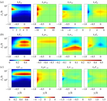


 Open access