2. Numerical set-up

To save computational resources, we analyse simulations of a pressure-driven turbulent open channel flow in a doubly periodic domain, between a no-slip wall at $y=0$ and an impermeable free-slip wall at $y=h$. The streamwise, wall-normal and spanwise directions are $x$, $y$ and $z$, respectively, and the corresponding velocities are $u$, $v$ and $w$, although position and velocities are occasionally denoted by their components $\boldsymbol {x}=\{x_j,\ j=1,2,3\}$. The domain size is $L_x\times L_y\times L_z={\rm \pi} h \times h \times {\rm \pi}h$, and the Reynolds number is $Re_\tau =u_\tau h/\nu =600.9$. The ‘$+$’ superscript denotes wall units, normalised with the friction velocity $u_\tau$ and with the kinematic viscosity $\nu$. Capital letters, as in $U(y)$, denote variables averaged over the simulation ensemble and over wall-parallel planes; lowercase letters are fluctuations with respect to this average, and primes are root-mean-square fluctuation intensities. Repeated indices, including squares, imply summations unless noted otherwise. The simulation code is standard dealiased Fourier spectral along $x$ and $z$, as in Kim, Moin & Moser (Reference Kim, Moin and Moser1987), but uses seven-points-stencil compact finite differences for the wall-normal derivatives, as in Hoyas & Jiménez (Reference Hoyas and Jiménez2006). Time marching is semi-implicit third-order Runge–Kutta (Spalart, Moser & Rogers Reference Spalart, Moser and Rogers1991), and the mass flux is kept constant. The numerical $y$ grid is stretched at the no-slip wall with a hyperbolic tangent. See table 1 for other numerical parameters.

Table 1. Computational parameters: $L_{i}$ is the domain size along the $i$th direction, $h$ is the ‘half-channel’ height, equivalent to the domain height in open channels, and $U_b$ is the bulk velocity. The grid dimensions $N_i$ and effective resolutions $\Delta {x_i}$ are expressed in terms of Fourier modes.

Figure 1(a) compares the resulting fluctuation profiles with existing data from regular and open channels. It was shown by Lozano-Durán & Jiménez (Reference Lozano-Durán and Jiménez2014a) that a computational box with $L_z/h={\rm \pi}$ reproduces well the statistics of regular channels, and figure 1 shows that the same is true for open ones. In particular, figure 1(b) shows that the spanwise kinetic energy spectrum fits well within the computational box. On the other hand, the figure shows that open and full channels agree only below $y/h\approx 0.5$, above which the effect of ‘splatting’ at the top wall is particularly visible in the fluctuations of the cross-flow velocities (Perot & Moin Reference Perot and Moin1995). We will use only the range $y^+\lesssim 300$ for the rest of the paper. It is also clear from the figure that the energy at long wavelengths above $y^+=100$ is higher than in del Álamo & Jiménez (Reference del Álamo and Jiménez2003). This is due to the short computational box, which inhibits the instability of the streaks (Abe, Antonia & Toh Reference Abe, Antonia and Toh2018), and results in two pairs of large streamwise streaks and rollers that dominate the flow.

Figure 1. (a) Velocity fluctuation intensities. Symbols represent the open channel at $Re_\tau =601$; dashed lines represent the open channel at $Re_\tau =541$ (Pirozzoli Reference Pirozzoli2023); and solid lines represent the full channel at $Re_\tau =547$ (del Álamo & Jiménez Reference del Álamo and Jiménez2003). Black indicates $u'$, red indicates $v'$, and blue indicates $w'$. (b) Premultiplied spanwise spectrum of the turbulent kinetic energy, normalised with $u_\tau ^2$. Contours are logarithmically equispaced from $k_zE_{KK}/u_\tau ^2=0.56$–2.8. The heavier vertical line is the present computational box. The thinner vertical line is $\lambda _z=2{\rm \pi} /k_z=h$, and the horizontal line is $y^+=300$. Filled contours are the present simulation; lines are from del Álamo & Jiménez (Reference del Álamo and Jiménez2003).

The original code was ported to CUDA by Vela-Martín et al. (Reference Vela-Martín, Encinar, García-Gutiérrez and Jiménez2021) for the efficient simulation of high-Reynolds number channel turbulence on GPU clusters. It has been adapted to a single GPU for the present experiments, but the original reference should be consulted for full details.

2.1. The initial perturbations

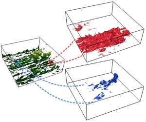
As mentioned in the Introduction, the interventional identification of causality follows (Jiménez Reference Jiménez2018b, Reference Jiménez2020b). The idea is to apply a spatially localised initial perturbation to existing turbulence, after which the flow is allowed to develop freely (see figure 2). The effect is measured after some time. Unlike the sensitivity analysis of the mean velocity profile in Farano et al. (Reference Farano, Cherubini, Robinet and De Palma2017), each causality experiment is the response to a particular perturbation on a particular location of a given flow snapshot, and the numerical experiment has to be repeated many times for different snapshots and perturbations. The goal is to create a database of responses from which to extract the characteristics that make a particular flow location influential for the future behaviour of turbulence (i.e. causally significant). To ensure independence, the 40 initial reference snapshots used for our experiments are separated by at least 1.4 turnovers (defined as $h/u_\tau$).

Figure 2. Schematic of the numerical experiment. Green represents the isosurface of the turbulent kinetic energy for the reference flow at $t=0$, $|\boldsymbol {u}_{\it ref}|^+=4.5$. Colour intensity encodes the distance from the wall. Red represents the perturbation kinetic energy at some later time, $|\boldsymbol {u}_{\it ref}(T)-\boldsymbol {u}_{\it mod}(T)|^+=0.17$, for a causally significant perturbation. Blue represents the same for a causally irrelevant perturbation.

Perturbations modify the flow within a cubical cell of side $l_{cell}$ centred at $\boldsymbol {x}_c$. Although there are countless choices for the form of the disturbance, and even if experience shows that the manner in which the flow is disturbed influences the outcome of the experiment (Jiménez Reference Jiménez2020b; Encinar & Jiménez Reference Encinar and Jiménez2023), cost considerations limit us to a single perturbation scheme. Specifically, the flow is modified by removing the velocity fluctuations within the cell, overwriting the velocity field with its $y$-dependent cell average. Defining the $y$-dependent cell average of a variable $f$ as

(2.1)\begin{equation} \overline{f}^{c}(y)=l_{cell}^{{-}2} \int^{x_c+l_{cell}/2}_{x_c-l_{cell}/2} \int^{z_c+l_{cell}/2}_{z_c-l_{cell}/2}{f(x,y,z)\,{\rm d}{\kern0.8pt}x\,{\rm d} z}, \end{equation}

the perturbed velocity $\boldsymbol {u}_{\it mod}$ is

(2.2)\begin{equation} \boldsymbol{u}_{\it mod} = \begin{cases} \overline{\boldsymbol{u}_{\it ref}}^{c} & \textrm{when}\ |x_j-x_{cj}|\leq l_{cell}/2,\\ \boldsymbol{u} _{\it ref} & \textrm{otherwise}, \end{cases} \end{equation}

where $\boldsymbol {u}_{\it ref}$ is the unperturbed flow, and an extra pressure step is applied after (2.2) to restore continuity at the edges of the cell. The experiment is repeated as many times as possible, applying it to different reference flow fields while changing the location and size of the perturbation cell.

Table 2 summarises the parameters of the experimental cells. They are expressed in terms of the distance from the wall to the bottom of the cell, $y_{cell}= y_c-l_{cell}/2$, which was found to collapse some results better than the cell centre, and are separated into two sets. In the first set, involving the 40 reference snapshots, perturbations are applied to a $6\times 6$ grid of cells evenly spaced in $x$ and $z$, such that their centres are separated by ${\rm \pi} h/6$ in each direction (approximately 315 wall units). In the $y$-direction, perturbations are applied at the heights detailed in the second column of table 2, ranging from cells touching the wall to those centred at the middle of the computational domain, $y_c^+\approx 300$. Each of them is run for 0.65 turnovers, and consumes approximately 6 minutes in an Nvidia A100 GPU, so that the approximately 76 000 experiments in this set took 318 GPU-days.

Table 2. Parameters of the perturbation cells. See text for details.

While these experiments test a wide range of sizes at sparsely spaced locations across the flow, the ones in the last column of table 2 aim to build heat maps that explore possible large-scale causality distributions not limited to a single cubical cell. Each reference snapshot is divided into a $30 \times 30$ grid in the $x$–$z$ plane, approximately spaced by 75 wall units, and perturbations are centred at each point of that grid. For cells with $l_{cell}^+\ge 75$, this procedure uniformly samples the whole plane, but due to its cost, it was limited to 20 initial snapshots and five different heights, each of which ran for only 0.49 turnovers. The resulting 180 000 tests took 565 GPU-days.

In both sets of experiments, the temporal evolution of the perturbation is measured by the energy of the perturbation velocity integrated over the whole computational domain,

(2.3)\begin{equation} \varepsilon_{\boldsymbol{u}} (t) = V^{{-}1}\int {|\boldsymbol{u}_{\it mod} - \boldsymbol{u}_{\it ref}|^2 \,{\rm d} V}, \end{equation}

which evolves from some initial $\varepsilon _{\boldsymbol {u}} (0)$ at the moment at which the perturbation is applied, to $\varepsilon _{\boldsymbol {u}}(\infty )=2 K\equiv 2V^{-1} \int |\boldsymbol {u}|^2 \,{\rm d} V$ when the reference and perturbed flow fields decorrelate after a sufficiently long time. For a chaotic system such as turbulence, $\varepsilon _{\boldsymbol {u}}(\infty ) \gg \varepsilon _{\boldsymbol {u}}(0)$, and even if the evolution of the perturbation is far from linear over times of the order of a turnover, the perturbation energy typically grows almost exponentially for a while before levelling at $\varepsilon _{\boldsymbol {u}}(\infty )$. These considerations lead to two definitions of causal significance: an absolute one that disregards the initial perturbation magnitude and vanishes as $t\to \infty$,

(2.4)\begin{equation} \sigma_{\boldsymbol{u}} (t) = \log_{10} \varepsilon_{\boldsymbol{u}}(t) / \varepsilon_{\boldsymbol{u}}(\infty)=\log_{10} \varepsilon_{\boldsymbol{u}}(t) / 2K, \end{equation}

and a relative one,

(2.5)\begin{equation} \sigma_{\boldsymbol{u}r} (t) = \log_{10} \varepsilon_{\boldsymbol{u}}(t) /\varepsilon_{\boldsymbol{u}}(0), \end{equation}

which measures relative growth and vanishes at $t=0$. Both definitions typically grow with time, but we will be interested in cases in which the growth is particularly fast or slow, as defined by the top and bottom $\phi$ percentile of the significance distribution. For most of the paper, experiments within the top $\phi =10\,\%$ of the significance distribution will be defined as ‘causally significant’, and those in the bottom 10 %, as ‘causally irrelevant’. This fraction is broadly compatible with the percolation analysis often used to define thresholds. For example, the optimal percolation threshold in three-dimensional wall-bounded turbulence fills volume fractions of the order of 5 %–10 % (Jiménez Reference Jiménez2018a), while in two-dimensional vorticity fields, which are more directly comparable with the present application to individual planes, the covered area is closer to 20 %–30 % (Jiménez Reference Jiménez2020a). Tests using $\phi =5\,\%$ or 15 % showed few differences in the present results.

3. Temporal evolution of the significance

To further study the growth of the perturbations, we use its $y$-dependent averaged intensity,

(3.1)\begin{equation} {\varepsilon_{\boldsymbol{u}}}(y,t)=(L_xL_z)^{{-}1}\iint |\boldsymbol{u}_{\it mod} - \boldsymbol{u}_{\it ref}|^2 \,{\rm d}{\kern0.8pt}x \,{\rm d} z, \end{equation}

equivalent to (2.3) but integrated over wall-parallel planes instead of over the whole domain, together with corresponding definitions for the significances. To minimise notational clutter, we use for them the same symbols as in (2.3)–(2.5), with the inclusion of $y$ as a parameter. Figure 3(a) shows the growth of $\varepsilon _{\boldsymbol {u}}(y)$, unconditionally averaged over all the perturbations introduced at a particular size and distance from the wall and normalised with its maximum at $t=0$. The blue line is the position at which the perturbation is maximum. It initially stays at the height at which the perturbation is introduced, but a new peak grows near the wall and becomes dominant after $tu_\tau /h\approx 0.3$. In figure 3(b), where the perturbation is initially attached to the wall, the peak is always attached. During the very early stage of evolution $(tu_\tau /h\lesssim 0.05)$, a low-intensity perturbation spanning the whole channel appears in both cases. This is most likely due to the pressure pulse that enforces continuity at the edges of the perturbation cell, but it quickly dissipates and does not seem to influence later development.

Figure 3. Plane-averaged perturbation magnitude ${\langle \varepsilon _{\boldsymbol {u}}\rangle }(y,t)$, as defined in (3.1), unconditionally averaged over all perturbations with $l_{cell}^+=75$ introduced at a given height, normalized with its maximum at $t=0$. The blue line is the instantaneous position of the perturbation maximum. Contours are ${\langle \varepsilon _{\boldsymbol {u}}\rangle }(y,t)/\max _y\langle \varepsilon _{\boldsymbol {u}}\rangle (y,0)$. Here, (a) $y_c^+=300$, (b) $y_{cell}=0$.

Figure 4 shows the attachment time $t_{att}$, defined for individual tests as the moment when the perturbation maximum falls below $y^+=50$, and later averaged over the experimental ensemble. It is approximately proportional to $y_{cell}$, at least for $y_{cell}^+\gtrsim 50$, with a propagation velocity ${\rm d}{\kern0.9pt}y_{cell}/{\rm d} t=1.37u_\tau$. This is faster than the observed vertical advection velocity of coherent features in channels, ${\rm d}{\kern0.9pt}y/{\rm d} t\approx \pm u_\tau$ (Lozano-Durán & Jiménez Reference Lozano-Durán and Jiménez2014b), and suggests that the perturbation is not simply advected by the flow, but actively amplified by it. In fact, the production term in the evolution equation for the perturbation energy is proportional to the mean shear (see Appendix A), and the most likely interpretation of figure 4 is that while all perturbations are advected to and from the wall by the background turbulence, those approaching the wall, where the shear is most intense, grow faster than those moving away from it, resulting in a mean downwards migration of the perturbation maximum. Notice, for example, the different slopes of downwards and upwards contours in figure 3. It is also relevant that $t_{att}$ scales better with the distance from the wall to the bottom of the cell, $y_{cell}$, than with its centre, $y_c$ (not shown), because it is the bottom that predominantly feels the stronger shear near the wall.

Figure 4. Attachment time $t_{att}$ as a function of $y_{cell}$, for different $l_{cell}$. The dashed line is a least-squares fit to the curves with $y_{cell}>0$, with slope ${\rm d}{\kern0.9pt}y/{\rm d} t=1.37u_\tau$. Times are computed for individual tests, and symbols and bars are their averages and standard deviations. Symbols are as in table 2.

Figures 5(a,b) show two examples of the temporal evolution of the domain-integrated perturbation $\varepsilon _{\boldsymbol {u}}$, using different cell sizes, and the line colour is the cell height. The figures show that $\varepsilon _{\boldsymbol {u}}$ is higher for larger cells, which is to be expected since it is an integrated quantity, and also for lower $y_{cell}$, also expected for a perturbation that removes velocity fluctuations, which are stronger near the wall. More interesting is that cells near the wall grow faster than those away from it, which may be understood as supporting the model in which their growth rate is controlled by the ambient shear.

Figure 5. Temporal development of the unconditionally averaged domain-integrated perturbation $\varepsilon _{\boldsymbol {u}} (t)$, as defined in (2.3), for (a) $l_{cell}^+=50$, (b) $l_{cell}^+=100$. In both plots, the cell distance from the wall increases from cold to warm colours, for the cases in table 2, and the diagonal dashed lines are the exponential Lyapunov growth rates from Nikitin (Reference Nikitin2018).

The dashed straight lines in figure 5 are the exponential growth rates from the Lyapunov analysis by Nikitin (Reference Nikitin2018), who reports a Lyapunov time for $\varepsilon _{\boldsymbol {u}}$ (the inverse of the leading exponent) of $T_L^+\approx 19$ ($u_\tau T_L/h=0.032$) in a turbulent channel at $Re_\tau =586$. The leading Lyapunov vector is concentrated in the buffer layer, and the exponent scales in wall units, again consistent with a model in which the growth is controlled by the near-wall shear.

It is clear that our analysis shares many characteristics with the classical Lyapunov analysis, albeit with important differences. The most obvious is that the classical Lyapunov exponent assumes that the perturbation behaves linearly for an infinitely long time, while figure 5 shows that our experiments saturate for times that, even if much longer than $T_L$, remain of interest for the flow evolution. A second important difference is that our initial perturbations, which are intended to probe the local structure of the flow rather than its mean properties, are compact with predetermined shapes, while those in Lyapunov analysis are allowed to spread across the flow field to their optimal structure. It may be relevant in this respect that there is an initial transient in which perturbations decay in most of our tests, $u_\tau t/h\lesssim 0.1$, and that this period is shorter for cells near the wall. This is reminiscent of the similar transient in Lyapunov calculations, during which perturbations align themselves to the most unstable direction. Our limited range of initial conditions is probably partly compensated by the substitution of the temporal averaging of classical analysis by averaging over tests, and it is interesting that the short-time growth rates of the smallest perturbations in figure 5(a), which mostly sample the buffer layer, approximately agree with Nikitin (Reference Nikitin2018). Larger or higher perturbations, which sample weaker shears, grow more slowly. We will provide in § 5.1 further support for the relevance of local shear to perturbation growth.

Figure 6(a) shows a typical evolution of the absolute significance $\sigma _{\boldsymbol {u}}$ for perturbations with a given $l_{cell}$ and $y_{cell}$. Each of the grey lines is the result of a different experiment, and the red and blue lines are the mean evolutions of samples that are respectively classified as significant or irrelevant at $t=0$. The bands are their standard deviations. The figure shows that the perturbations approximately maintain the ordering of their initial intensity. Initially stronger perturbations tend to remain strong for long times, although it follows from its definition that $\sigma _{\boldsymbol {u}}$ vanishes on average as $t\to \infty$. Figure 6(b) displays the persistence of the causality classification based of $\sigma _{\boldsymbol {u}}$, defined as the fraction of samples identified as significant or irrelevant at $t=0$ that remain significant or irrelevant when classified at subsequent times. In the case illustrated in the figure, 34 % of the initially significant samples, and 29 % of the initially irrelevant ones, remain at the end of our experiments in the same class in which they were classified at $t=0$. This fraction is at least 20 % in all the experiments in this paper, which is substantially higher than the 10 % expected from a random selection.

Figure 6. (a) Grey lines are the absolute significance $\sigma _{\boldsymbol {u}}$ (2.4) for individual experiments, as a function of time; only 20 % of the total are included. The red and blue lines and their corresponding bands respectively represent the mean evolution and standard deviation of the samples diagnosed as significant or irrelevant at $t=0$. (b) Fraction of experiments that continue to be classified as significant or irrelevant in terms of $\sigma _{\boldsymbol {u}}$ at different times, after being so classified at $t=0$. Red indicates significant; blue indicates irrelevant. The black horizontal line is the probability threshold $\phi =10\,\%$. (c) As in (a), for the relative significance $\sigma _{\boldsymbol {u}r}$ (2.5) diagnosed at $tu_\tau /h=0.29$. In all cases, $l_{cell}^+=50$, $y_{cell}^+=125$.

Figure 6(c) shows the evolution of the relative significance. Unlike the absolute significance, $\sigma _{\boldsymbol {u}r}$ vanishes at $t=0$ but does not reach the same long-time limit in all cases. In fact, $\sigma _{\boldsymbol {u}r}(\infty ) = \log _{10} (2K) - \log _{10} \varepsilon _{\boldsymbol {u}}(0)$, and $\sigma _{\boldsymbol {u}r}(\infty )$ is essentially equivalent to the initial perturbation magnitude.

These considerations show that both $\sigma _{\boldsymbol {u}}$ and $\sigma _{\boldsymbol {u}r}$ characterise the evolution of the perturbations at short and intermediate times. The former mostly reveals that the perturbation intensity stays approximately proportional to its initial value for some time, while the latter, which compensates for this effect, describes its intrinsic growth. When $\varepsilon _{\boldsymbol {u}}\to 2K$ at longer times, the system forgets its initial conditions, and neither measure of significance is very useful.

Although figure 6(b) shows that the significance classification of a given experiment is not a completely random variable, the fact that the persistence is not unity implies that the time at which the classification is performed is important. Consider, for example, the mean significance of the set $\{I\}$ of tests classified at time $t_c$ as irrelevant, $\sigma _I(t_c) =N_{\{I\}}^{-1} \sum _{j\in \{I\}} \sigma _j$, and define a similar $\sigma _S (t_c)$ average for significant perturbations. The difference $\sigma _S-\sigma _I$ typically increases initially and reaches a maximum before decaying at long times. The time $t_{sig}$ at which this difference is maximum is also when the classification is less ambiguous, and we will preferentially use it from now on to define our significance classes.

Figures 7(a,b) show how $t_{sig}$ changes as a function of $l_{cell}$ and $y_{cell}$, using either $\sigma _{\boldsymbol {u}}$ or $\sigma _{\boldsymbol {u}r}$ as a causality measure. Disregarding the case $l_{cell}^+=25$, which is well within the dissipative range of scales and tends to behave differently from larger cells, $t_{sig}$ is explained mainly by $y_{cell}$, and it is clear that $\sigma _{\boldsymbol {u}r}$ is a better indicator for this purpose than $\sigma _{\boldsymbol {u}}$. We will mostly use it from now on. It is interesting that $t_{sig}$ is very close to, and generally slightly larger than, the attachment time $t_{att}$ in figure 4, as shown by the difference of the two values in figure 7(c), suggesting again that the arrival of the disturbances to the wall is an important factor in determining causality.

Figure 7. Optimal classification time $t_{sig}$ as a function of $y_{cell}$. Symbols as in table 2. The dashed lines in (a,b) are least-squares linear fits, whose slope is ${\rm d}{\kern0.9pt}y/{\rm d} t=2.12 u_\tau$ in (a) and ${\rm d}{\kern0.9pt}y/{\rm d} t=1.28 u_\tau$ in (b). (a) Using $\sigma _{\boldsymbol {u}}$; (b) using $\sigma _{\boldsymbol {u}r}$. (c) Offset between the $\sigma _{\boldsymbol {u}r}$ classification time and the attachment time.

We have seen above that the initial intensity of the perturbations has an effect on their subsequent evolution. This is also true of our significance classification, and can be quantified by the correlation of $\sigma _{\boldsymbol {u}r}(t_c)$ with $\varepsilon _{\boldsymbol {u}}(0)$ (not shown). This correlation tends to $-1$ at long times, as explained above, but remains moderately positive for $t_c\lesssim t_{sig}$, confirming that the initial relative growth rate for strong perturbations is faster than for weak ones. In most cases, $t_{sig}$ approximately coincides with the moment at which the correlation changes sign and is close to zero, making the classification relatively independent of the initial perturbation intensity. At this moment, the energy of the perturbation is still a small fraction of the total energy of the flow. Taking as an example the topmost curve in figure 5(b) $(l_{cell}^+=100$, $y_{cell}=0)$, the average energy of the initial perturbations is approximately $3\times 10^{-4}\,{K}$, and grows to $0.6K$ at the end of the experimental runs, but it is still $8\times 10^{-3}\,{K}$ at the optimal classification time $t_{sig}\approx 0.17{ h}/u_\tau$. This does not mean that the perturbation can be linearised up to that time. The intensity of the perturbation is always $O(K)$, and the growth of its integrated energy is mostly due to its geometric spreading (see figure 2).

4. Diagnostic properties for causal significance

Having described how the significance of an initial condition can be characterised, we recover our original task of determining which properties of the perturbed cells are responsible for their causality. The basic assumption is that the characterisation of causality can be reduced to a single observable of the cell at the perturbation time, $t=0$, such as its average vorticity, rather than requiring several conditions to be satisfied simultaneously, or even some property of the extended environment of the cell, or of its history. As mentioned in the Introduction, the strategy is to perform many experiments modifying individual cells, to label them according to their significance at some later time, and to test which cell observables at $t=0$ can be used to separate the classes thus labelled. Hereafter, the one-point scalar $\langle\, f\rangle _{c}$ stands for the cell average of a property:

(4.1)\begin{equation} \langle\,f\rangle_{c}=l_{cell}^{{-}3} \int^{y_{cell}+l_{cell}}_{y_{cell}} \int^{x_c+l_{cell}/2}_{x_c-l_{cell}/2}\int^{z_c+l_{cell}/2}_{z_c-l_{cell}/2}{f(x,y,z) \,{\rm d}{\kern0.8pt}x \,{\rm d}{\kern0.9pt}y \,{\rm d} z}. \end{equation}

Following Jiménez (Reference Jiménez2020b) and Encinar & Jiménez (Reference Encinar and Jiménez2023), the ranking of observables uses a linear-kernel support vector machine (SVM) (Cristianini & Shawe-Taylor Reference Cristianini and Shawe-Taylor2000), implemented in the scikit-learn Python library (Pedregosa et al. Reference Pedregosa2011), which determines an optimal separating hyperplane between two pre-labelled data classes. In our case, we look for the optimal separation of significant or irrelevant experiments in terms of a single quantity, and the SVM hyperplane reduces to a threshold. For each combination of $l_{cell}$ and the $y_{cell}$ values in the second column of table 2, and for each classification time $t_c$, two-thirds of the initial conditions are collected into a training set, with the remaining third reserved for testing. The 10 % most significant experiments of the training set are labelled as significant, and the bottom 10 %, as irrelevant. The remaining 80 % are not used for classification purposes. An optimum partition threshold is computed for each of the observables detailed below, and an SVM classification score is assigned to each observable using the test set. The score measures the fraction of data allocated to their correct class by the SVM threshold, and ranges from unity for perfect separability to 0.5 for cases in which the two classes are fully mixed. The procedure is repeated three times after randomly separating the data into training and test sets, and the diagnostic score for the observable is defined as the average of the three results.

The whole process can be automated and is reasonably fast. The experimental description in § 2.1 shows that each SVM run is only requested to classify two sets of 96 points each, and to test the classification on two sets of 48 points. This allows us to minimise pre-existing biases by testing many possible observables. The robustness of the classification results was assessed by decreasing the number of samples by half.

The observables can be physically classified into average cell properties, such as kinetic energy, and perturbation or small-scale properties, such as the kinetic energy of the velocity fluctuations with respect to the cell mean. The former are summarised in table 3, and the latter in table 4. In both cases, properties that are statistically symmetric with respect to reflections on $z$ are used as absolute values, and positive definite quantities, such as mean squares, are used as logarithms. Otherwise, all observables are processed in the same way.

Table 3. Cell observables. All averages are taken over cells at $t=0$.

Table 4. As in table 3, for observables describing perturbation and small-scale quantities.

The diagnostic score of an initial condition depends on the cell height, on its size, and on the moment at which it is classified. Figure 8 shows a typical table of the three best observables identified by the absolute significance $\sigma _{\boldsymbol {u}}$, as functions of the classification time. Cells are coloured by the classification score. In all cases, the best observable is the initial perturbation amplitude $\varepsilon _{\boldsymbol {u}}$, a related quantity such as $\varepsilon _{\boldsymbol {\omega }}$, or the viscous dissipation of the perturbation intensity $\langle {D_{\varepsilon u}}\rangle _{c}$. Although not included in the table, the next best observable is usually also a small-scale quantity closely correlated with the intra-cell velocity fluctuations, such as $s_{ij}s_{ij}$, $\omega _i^2$ or the in-cell standard deviation ${v}^{\prime c}$. The table in figure 8 is thus equivalent to the fluctuation persistence in figures 6(a,b).

Figure 8. Classification score of the three best observables for a classification based on absolute significance $\sigma _{\boldsymbol {u}}$. Row indicates rank; column indicates evaluation time in turnovers. The highlighted column is $t_{sig}$. Colour indicates the classification score. Here, $l_{cell}^+=50$, $y_{cell}^+=125$.

In the sense that this absolute persistence is due to the slow relaxation of the initial amplitude, it can be considered physically uninteresting, but it can be largely compensated by using the relative significance $\sigma _{\boldsymbol {u}r}$ defined in (2.5). Figure 9 displays the two best observables for different sizes at a fixed cell height, and figure 10 displays results for a given size and different heights. In both cases, the best score starts being relatively high at short classification times, decreases for intermediate ones, and increases again towards the end of the experimental run. The evolution of the optimum diagnostic variables with the classification time can be divided into three phases.

Figure 9. Classification score of the two best observables for a classification based on relative significance $\sigma _{\boldsymbol {u}r}$: (a) $l_{cell}^+=150$, $y_{cell}^{+}=150$, (b) $l_{cell}^+=75$, $y_{cell}^{+}=138$, (c) $l_{cell}^+=25$, $y_{cell}^+=138$. Row indicates rank; column indicates evaluation time in turnovers. The highlighted columns are $t_{sig}$. Colour indicates classification score. Here, $y_{cell}^+\approx 150$.

Figure 10. Classification score of the two best observables for a classification based on relative significance $\sigma _{\boldsymbol {u}r}$: (a) $y_{cell}^+=275$, (b) $y_{cell}^+=125$, (c) $y_{cell}=0$. Row indicates rank; column indicates evaluation time in $h/u_\tau$. The highlighted columns are $t_{sig}$. Colour indicates classification score. Here, $l_{cell}^+=50$.

During the initial phase, up to the time when the scores are lowest, the best observables include $s_{ij}s_{ij}$, the magnitude of the initial disturbance, and the disturbance production and dissipation, all of which are either highly correlated with the initial value of $\varepsilon _{\boldsymbol {u}}$, or are terms in its evolution equation (A8). This part of the table is equivalent to the observation in § 2.1 that initially stronger perturbations not only remain strong, but also grow faster than weaker ones.

The second phase is the broad minimum of the score around $t_{sig}$. While the scores in this phase are not high, the best observables change from the small-scale perturbation properties of the initial phase to properties of the cell that do not include fluctuations, such as the cell average of some velocity component, or equivalently, the mean shear when the cells are very close to the wall. It is interesting that the best measure of shear near the wall is $\langle \partial _y u\rangle _{fw}$, which excludes the viscous sublayer (see figure 10c). This is consistent with the idea that the growth of the perturbation is due to the energy production by the local shear, because the fluctuation production term in Appendix A is proportional to the shear, but also to the Reynolds stresses $\hat {u}_i\hat {u}_j$, which are inactive in the sublayer.

It is interesting that the longitudinal velocity derivatives $\langle {\partial _x u}\rangle _{c}$ and $\langle {\partial _z w}\rangle _{c}$ appear among the most diagnostic cell properties for wall-attached perturbations in figure 10(c). These derivatives are involved in mass conservation, and follow naturally from the meandering of near-wall streaks, which has been associated with streak breakdown (Jiménez & Moin Reference Jiménez and Moin1991; Hamilton et al. Reference Hamilton, Kim and Waleffe1995; Waleffe Reference Waleffe1997) and with the generation of Orr bursts (Orr Reference Orr1907; Jiménez Reference Jiménez2013). Although not apparent from figure 10(c), it can be shown that significant cells are associated with $\partial _x u<0$, $\partial _z w>0$, with the opposite association for irrelevant ones.

Finally, at longer times of the order of $t-t_{sig} \approx 0.25h/u_\tau$, the score recovers, and the most diagnostic observable reverts to the small-scale quantities that dominate short times. Since we saw in § 2.1 that $\sigma _{\boldsymbol {u}r}$ at long times is essentially equivalent to $\varepsilon _{\boldsymbol {u}}(0)$, this final phase is a reflection of the behaviour at short times, and does not represent new physics.

Figure 11(a) shows the dependence on $y_{cell}$ of the time at which the accumulated score of the top four observables reaches its minimum. After an initial transient that gets shorter as the cell size increases, $t_{min}$ grows with the distance from the wall, and approximately tracks the optimum classification time $t_{sig}$.

Figure 11. (a) The solid lines are the time $t_{min}$ at which the sum of the scores of the four best observables is lowest. The dashed lines are $t_{sig}$ from figure 7(b). Other symbols are as in table 2. (b–f) Classification scores of selected observables as functions of time, computed from $\sigma _{\boldsymbol {u}r}$. Crosses indicate small-scale quantities, defined as the average of the scores of $\varepsilon _{\boldsymbol {u}}$ and $\langle {s_{ij}s_{ij}}\rangle _{c}$. Triangles indicate cell-scale quantities, average of $\langle {u}\rangle _{c}$ and $\langle {v}\rangle _{c}$. Abscissae are offset by the attachment time $t_{att}$. Colour intensity increases with the distance from the wall, from $y_{cell}^+=12.5$ to $y_{cell}^+=275$, with (b) $l_{cell}^+=25$, (c) $l_{cell}^+=50$, (d) $l_{cell}^+=75$, (e) $l_{cell}^+=100$, ( f) $l_{cell}^+=150$.

Figures 11(b–f) summarise the evolution of the scores as functions of time. The blue lines are averages of the scores of several fluctuation quantities, and the red lines are averages of cell-scale properties. The figures are offset by their attachment time $t_{att}$, which improves their collapse significantly, and reflect the decreasing influence of the small-scale quantities as the perturbations approach the attachment time, as well as the increasing importance of the cell-scale properties as the perturbations intensify. It should be mentioned that offsetting $t$ with the optimum classification time $t_{sig}$, instead of with $t_{att}$, also collapses most scores, as could be expected from the similarity of both times in figure 7. It also collapses better the case $y_{cell}=0$, which is not included in figure 11, and for which $t_{att}$, defined at the arbitrary distance $y^+=50$, does a poor job. In spite of this, $t_{att}$ is used in figure 11 because it improves the case $l_{cell}^+=25$, and underscores the already mentioned connection between significance and the energy production from the near-wall shear. It is also interesting that the score of the velocities has a secondary maximum at $t=0$, probably due to the known correlation of small-scale vorticity with the large-scale streamwise-velocity streaks (Tanahashi et al. Reference Tanahashi, Kang, Miyamoto, Shiokawa and Miyauchi2004).

From now on, we will mostly focus on results of the relative significance classified at $t_{sig}$, for which the optimum observables are collected in figure 12. As seen above, they are mostly the average cell velocities, $\langle {u}\rangle _{c}$ or $\langle {v}\rangle _{c}$. The exceptions are cells in the buffer layer $y_{cell}^+\lesssim 50$, in which shear can probably be taken as a proxy for the streamwise velocity, and cells with $l_{cell}^+=25$ very far from the wall. We have already mentioned that these perturbations are probably too small to survive for the relatively long times required to reach the wall, in agreement with the assimilation results from Wang & Zaki (Reference Wang and Zaki2022) mentioned in the Introduction.

Figure 12. Best observable at $t_{sig}$. Colour indicates score. The bottom of each tile in the figure aligns with the left-hand $y_{cell}$ axis.

5. Conditional flow fields

While we have seen that the cell-averaged velocity fluctuations are diagnostic quantities for causality, our analysis did not include their sign. Figures 13–15, which display averaged velocity fields conditioned to the position of significant or irrelevant perturbation cells, shows that the sign is important.

Figure 13. Streamwise section at $z=z_c$ of the conditional velocity field of the reference flow at $t=0$ around the perturbation cell. The colour background is the conditional streamwise velocity. Arrows are velocity fluctuation vectors parallel to the plane of the figure, and the light-coloured box is the perturbation cell. Here, $l_{cell}^+=75$, and (a,b) $y_{cell}^+=113$, (c,d) $y_{cell}^+=62.6$, (e,f) $y_{cell}=0$. (a,c,e) Significants, (b,d,f) irrelevants.

Figure 13 displays longitudinal ($x$–$y$) sections of the streamwise and wall-normal velocities, conditioned to either significant (figures 13a,c,e) or irrelevant (figures 13b,d,f) cells. It is evident that the former are biased towards fourth-quadrant regions ($u>0$, $v<0$), while the latter are in second-quadrant regions ($u<0$, $v>0$) (Lu & Willmarth Reference Lu and Willmarth1973).

The three rows in figure 13 corresponds to perturbations introduced at decreasing distances from the wall. The frames are centred at the streamwise position of the perturbation cell, and the figure shows a fluid wedge entering the frame from its downstream right-hand edge, becoming more prominent as the cell approaches the wall. At the same time, there is an upstream drift of the darker core of the velocity distribution. This is clearest in the significant cases in figures 13(a,c,e), where the incoming wedge is low-speed fluid, but it can also be traced in the irrelevant cases in figures 13(b,d,f). The result is that the position of the causally significant cells moves downstream towards an interface at which high-speed fluid overtakes a low-speed one. Irrelevants are associated to an interface in which low-speed fluid is left behind by higher speed ahead of it.

Figure 14 displays wall-parallel ($x\unicode{x2013}z$) sections of the same cases as figure 13, and figure 15 shows cross-flow ($z$–$y$) sections of figures 13(a,b). There is no orientation ambiguity in the longitudinal sections in figure 13, but figures 14 and 15 would be statistically symmetric even if individual flow fields were not. To preserve possible systematic asymmetries, the $z$ coordinate of all the flow fields is reflected so that the spanwise velocity averaged over a cube of side $3l_{cell}$, centred at the perturbation cell and possibly truncated by the wall, is $\langle w \rangle _{3c}<0$. The orientation of the sections in figures 14 and 15 is therefore not physically meaningful, but the asymmetry of the different frames is consistent and complements the information in figure 13.

Figure 14. As in figure 13, for a wall-parallel section at $y=y_c$.

Figure 15. As in figures 13(a,b), for the ($z$–$y$) cross-flow section at $x=x_c$. (a) Significants, (b) irrelevants, for $y_{cell}^+=113$, $l_{cell}^+=75$.

Figure 14 shows that the velocity interfaces in figure 13 correspond to kinks in the large-scale streaks that dominate the flow.

Although the frames in figures 13 and 14 represent unrelated experiments, it is tempting to interpret them as a temporal evolution in which perturbations introduced farther from the wall correspond to earlier times, and travel downstream and towards the wall until they reach it at $t_{att}$ (or $t_{sig}$). The velocity maximum in figures 14(a,c,e) shifts by $\Delta x^+\approx 200$ from the top to the bottom row of frames. Assuming, from figure 4, that $u_\tau t _{att}/h \approx 0.2$, this corresponds to a velocity difference $\Delta u^+\approx 1.5$, which is a reasonable estimate for the difference in the advection velocity of features in a high-velocity streak with respect to the average flow velocity (Krogstad, Kaspersen & Rimestad Reference Krogstad, Kaspersen and Rimestad1998; Lozano-Durán & Jiménez Reference Lozano-Durán and Jiménez2014b).

Interestingly, the streamwise drift of the irrelevant velocity features in the right-hand columns of figures 13 and 14 is less clear than in the significant ones in the left-hand columns. The environment of the irrelevants can rather be described as an interface that gets wider as the cell approaches the wall. The flow cross-sections in figure 15 support this description, and the combined evidence from the three sets of sections is consistent with a model in which causally significant cells are associated with the front of a high-speed sweep that steepens as it approaches the wall and overtakes a lower-speed region. Conversely, irrelevant cells are located at the trailing end of a high-speed region that leaves behind a lower-speed flow. We may recall at this point that the table in figure 10(c) showed that the wall-parallel mass conservation derivatives are diagnostic of causality near the wall, and that while $\partial _x u<0$ signals significance, $\partial _x u>0$ signals irrelevance. This asymmetry suggests that the generation of structures strong enough to have a global effect on the flow depends on mass conservation failures when streaks of different velocity run into each other. This is most probably due to meandering, as in figures 14(a,c,e), and the effect is strongest when this happens within the strong shear near the wall. The trailing edges of the meander, as in figures 14(b,d,f), or the tails at which high-speed streaks pull away from low-speed ones, are passive.

The association of strong near-wall $v$ structures with the downstream end of high-speed streaks and with the upstream end of low-speed ones was already noted by Jiménez, del Álamo & Flores (Reference Jiménez, del Álamo and Flores2004) and Jiménez & Kawahara (Reference Jiménez and Kawahara2013). Their interpretation was that $v$ creates the streaks, but the arguments above, together with the fact that causality can be traced to flow locations far from the wall, suggest that the sequence of events is the other way around, and that the formation of near-wall bursts depends on continuity failures of non-uniform $u$ streaks.

5.1. The shear time

Figure 16 is similar to the evolution of the plane-averaged fluctuation magnitude in figure 3, but is here separated into conditionally significant cases (filled contours) and irrelevant ones (lines). In both cases, as well as in the unconditional evolution in figure 3, the perturbation initially remains at the height at which it is introduced, before spreading vertically. All perturbations eventually fill the channel, as expected for a chaotic system, but the growth is faster in the significant cases. The bold cyan lines in figure 16 are the wall-normal position of the perturbation maximum. It is clear that the solid lines representing significants initially trend downwards and attach to the wall faster than the dashed lines representing irrelevants, which initially trend away from the wall or drift little. This supports the interpretation that significants are sweep-like, and the conjecture in §§ 3 and 4 that causal significance depends on the amplification of perturbations by the strong shear near the wall.

Figure 16. Plane-averaged perturbation magnitude ${\langle \varepsilon _{\boldsymbol {u}}\rangle }(y,t)$, as defined in (3.1), conditionally averaged over significant or irrelevant perturbations and normalised with the maximum of the conditioned initial value. The bold cyan lines are the instantaneous position of the perturbation maximum. Filled contours and the solid cyan line are significants; line contours and the dashed cyan line are irrelevants. Contour levels are ${\langle \varepsilon _{\boldsymbol {u}}\rangle }(y,t)/\max _y\langle \varepsilon _{\boldsymbol {u}}\rangle (y,0)$. Classification is done at $t_{sig}$ using $\sigma _{\boldsymbol {u}r}$, and $l_{cell}^+=75$, with (a) $y_{cell}^+=113$, (b) $y_{cell}^+=263$.

This is tested directly in figure 17. Figure 2 shows that perturbations spread with time along the three directions, and that it is difficult to define an instantaneous location to measure the shear that they encounter, but figures 3 and 16 suggest that it is possible to define an effective shear by weighting the mean velocity profile, which depends only on $y$, with the perturbation magnitude

(5.1)\begin{equation} S_\varepsilon (t)=\frac{\displaystyle\int \varepsilon_{\boldsymbol{u}}(y,t)\,\partial_y U(y)\,{\rm d}{\kern0.9pt}y}{\displaystyle\int \varepsilon_{\boldsymbol{u}}(y,t)\,{\rm d}{\kern0.9pt}y}, \end{equation}

and a dimensionless effective shear time

(5.2)\begin{equation} T_S (t)=\int{S_\varepsilon\,{\rm d} t}. \end{equation}

Figure 17(a) illustrates the development of the relative growth of causally significant and irrelevant perturbations in terms of the global eddy turnover time. The significant perturbations grow from the start, while the irrelevant ones initially decay and only later grow to match the causal case. Most of the initial decay and of the slow growth of irrelevants can be attributed to their failure to initially approach the wall. Figure 17(b) plots the same data using the local shear time computed for individual experiments. The two evolutions now approximately coincide, supporting the importance of the local shear, and providing an explanation for the association of sweep-like flows with causality. The effect of the negative wall-normal velocity is to bring perturbations close to the wall. Ejection-like regions move perturbations away from the wall to layers where the shear is low, and they become causally relevant only after they eventually diffuse into the near-wall layer.

Figure 17. Relative perturbation growth $\sigma _{\boldsymbol {u}r}(t)$ conditioned to significant (red) and irrelevant (blue) samples, classified at $t_{sig}$. Solid line indicates the mean; shading indicates the standard deviation; $\blacklozenge$ indicates $t_{sig}$. (a) In eddy turnovers; (b) normalised by the local shear time, as in (5.2). The dashed part of the irrelevant line in (b) corresponds to times for which not all experiments are available, because some of them end within the plot. Here, $l_{cell}^+=75$, $y_{cell}^+=133$.

The collapse with the shear time applies only to significant and irrelevant perturbations at the same distance from the wall. Perturbations introduced at different distances behave differently, at least at the relatively low Reynolds number of our experiments for which self-similar behaviours with respect to $y$ are necessarily limited.

5.2. Geometry of causal events

While we have seen that significant and irrelevant cells are associated with sweep- and ejection-like regions of the flow, it remains unclear whether the quadrants discussed in the previous section are the same as the intense events traditionally associated with sweeps and ejections in wall turbulence (Lu & Willmarth Reference Lu and Willmarth1973). This is the purpose of the experiments in the second column of table 2, which cover selected wall-parallel planes with a dense grid of perturbation experiments.

Figure 18 displays the resulting quadrant plot, drawn for cell-average quantities. The line contours are the unconditional joint probability density function of $\langle {u}\rangle _{c}$ and $\langle {v}\rangle _{c}$, while the coloured ones are conditioned to either significant cells in figure 18(a), or irrelevants in figure 18(b). The hyperbolic lines in the figure are intensity limits for sweeps and ejections, defined as

(5.3)\begin{equation} |\langle{u}\rangle_{c}(\boldsymbol{x})\,\langle{v}\rangle_{c}(\boldsymbol{x})|\ge H_\pm \langle{u}\rangle_{c}'(y)\,\langle{v}\rangle_{c}'(y).\end{equation}

In the classical quadrant plot for point velocities, the threshold $H$ depends only on $y$ (Lozano-Durán et al. Reference Lozano-Durán, Flores and Jiménez2012), and results in different volume fractions for sweeps and for ejections (see the last row of table 5). To facilitate comparison with our choice of a common area fraction for significant and irrelevant cells, figure 18 uses two different thresholds: $H_-$ for sweep-like structures with $\langle {v}\rangle _{c}<0$, and $H_+$ for ejection-like ones with $\langle {v}\rangle _{c}>0$. They are adjusted so that the total areas for sweeps and for ejections are the ones used for the significance analysis, $\phi =10\,\%$. They are given in table 2 for the five experimental wall distances, and are lower than the $H\approx 1.75$ used in Lozano-Durán et al. (Reference Lozano-Durán, Flores and Jiménez2012) and in other studies. Correspondingly, they select a larger area fraction, 20 % in total, rather than the approximately 9 % volume fraction in Lozano-Durán et al. (Reference Lozano-Durán, Flores and Jiménez2012). However, table 5 shows that the distribution of quadrants in these intense regions is not very different from the classical values, once the relative fractions of sweep- and ejection- like structures are taken into account. As in the case of point velocities, most strong structures are either pure sweeps, $\langle {u}\rangle _{c}>0$, $\langle {v}\rangle _{c}<0$, or pure ejections, $\langle {u}\rangle _{c}<0$, $\langle {v}\rangle _{c}>0$, and there are comparatively few intense $Q_1$ or $Q_3$. The filled contours in figure 18(a) are cell-averaged velocities of the significant cells, and those in figure 18(b) are irrelevant ones. It is evident that significants tend to be in strong $Q_2$ sweeps, while irrelevants are in strong $Q_4$ ejections.

Figure 18. Joint probability density function of the cell-averaged velocities. Line contours are unconditional. Filled ones are conditioned to (a) significant cells, (b) irrelevants. Both contain 60 % and 99 % of the data, and $y_{cell}^+=113$, $l_{cell}^+=75$. The solid hyperbolae are the $H_-$ threshold that isolates the 10 % most intense velocity quadrants with $\langle {v}\rangle _{c}<0$, as in (5.3), and the dashed hyperbolae are $H_+$ for $\langle {v}\rangle _{c}>0$.

Table 5. Parameters of intense quadrant structures for cell-averaged velocities, compiled over wall-parallel planes for $l_{cell}^+=75$. The thresholds $H_-$ and $H_+$ are as in figure 18, and the $S_j$ are the fraction of the intense area associated with each quadrant. The bottom row gives volume fractions for pointwise quadrant structures in the $Re_\tau =935$ channel of Lozano-Durán, Flores & Jiménez (Reference Lozano-Durán, Flores and Jiménez2012), in which the combined intense quadrants fill 9 % of the channel volume.

This association is quantified in figure 19. The area fraction of the intersection between two classes, $A$ and $B$, is defined as $\varGamma (A,B) = 2 S(A \cap B)/(S(A)+S(B))$, where $S$ denotes the area covered by each class. Figure 19(a) shows the intersection of significant structures with intense quadrants $Q_j$. The dashed lines are area fractions of the intersection of random $Q_j$ structures with the same area as the significance structures. Figure 19(b) repeats the analysis for irrelevants. It is again clear that significants predominantly overlap $Q_4$, and irrelevants overlap $Q_2$, with a maximum at $y^+\approx 100\unicode{x2013}150$.

Figure 19. Area fraction of the significance structures intersected by intense quadrants, for $l_{cell}^+=75$. Red indicates $Q_4$; blue indicates $Q_2$; black indicates $Q_1\cup Q_3$. Solid lines are conditioned to (a) significants, (b) irrelevants. Dashed lines are unconditional.

The question of whether significant cells are organised into structures similar to those of intense quadrants is addressed in figure 20. Each heat map displays the same plane away from the wall. Cells are shown at their position at $t=0$, but labelled by their relative significance evaluated some time after they are perturbed. The evaluation time increases from left to right. The heat map in figure 20(a) is featureless, reflecting the difficulty discussed in § 3 of predicting the future significance of a cell from its growth at short times. The organisation increases in figure 20(b), and is best developed in figure 20(c), where significance is evaluated at the optimum classification time $t_{sig}$. The size and organisation of the significance in figure 20(c) are very similar to those in the velocity maps in figures 14(a,b), with structures of $O(h)$ organised into longer streaky structures.

Figure 20. Heat maps of the relative significance $\sigma _{\boldsymbol {u}r}$ at various evaluation times. Note that the grid shows the position of the initial cells, whereas the colour indicates their relative significance evaluated at some future time. Here, $l_{cell}^+=75$, $y_{cell}^+=113$. Evaluation times (a) $0.01 h/u_\tau$, (b) $0.14 h/u_\tau$, (c) $0.28 h/u_\tau \approx t_{sig}$.

This suggests the possibility that irrelevants and significants are essentially the same as sweeps and ejections. To test this hypothesis, both sets of cells are collected into individual connected objects for which the product $\langle {u}\rangle _{c}\langle {v}\rangle _{c}$, or $\sigma _{\boldsymbol {u}r}$, is above or below the threshold required to isolate the $\phi \%$ area fraction of their wall-parallel plane, as in Lozano-Durán et al. (Reference Lozano-Durán, Flores and Jiménez2012). It is known that the wall-attached sweeps and ejections of the pointwise velocity form spanwise pairs (Lozano-Durán et al. Reference Lozano-Durán, Flores and Jiménez2012). A similar analysis is done here for the cell-averaged quadrants and for the significance structures. The centroid of all the structures and their pairwise distance is computed first, and two structures, such as $A_i$ and $B_j$, are defined as a pair if $B_j$ is the closest object to $A_i$, and $A_i$ is the closest object to $B_j$. It can be shown that the probability that significant and irrelevant structures are part of a close pair is similar to that for $Q_2$ and $Q_4$, and much larger than for randomly located objects.

Figure 21 presents joint probability density functions of the relative positions of the nearest structures of similar kinds. Filled contours depict irrelevants around significants, and lines indicate ejections around sweeps. Both use spanwise symmetry to enhance statistical convergence, and it is clear that the pairs of the two types of structures have a similar organisation. Figure 22 shows the average spanwise width of the pairs as a function of wall distance and cell size. It is known from Lozano-Durán et al. (Reference Lozano-Durán, Flores and Jiménez2012) that this width scales with $y$ for attached $Q_2$–$Q_4$ pairs far from the wall. Our Reynolds number is too low for this self-similarity to hold, but figure 22 shows that, at least for the two smallest cell sizes, the width of the significance pairs grows with the distance from the wall, and approximately follows that of the quadrants. It is difficult to make an exact correspondence between single planes and slabs of relatively large cells, and the green line in the figure is probably a reflection of this difficulty. Its cell size, $l_{cell}^+=150$, is of the same order as the distance from the wall. Similarly, the apparently large discrepancy of the $l_{cell}^+=75$ red line with the quadrant pairs at $y_{cell}=0$ is put in perspective by figure 21(a), which represents the same data.

Figure 21. Joint probability density function of the relative position $\{\delta _j\}$ of structures in close pairs. Filled contours are irrelevant–significant pairs, and lines are $Q_2$–$Q_4$. Contours contain 60 % and 99 % of the data, and $z$-symmetry is enforced. Here, (a) $y_{cell}^+=0$, (b) $y_{cell}^+=113$, (c) $y_{cell}^+=263$. In all cases, $l_{cell}^+=75$.

Figure 22. Mean spanwise distance among nearest significance or quadrant structures. Lines with symbols are significant–irrelevant pairs, with symbols denoting $l_{cell}$, as in table 2. The dashed line is $Q_2$–$Q_4$.

Finally, figure 23 shows the relative positions of intense quadrants with respect to significance structures. Figure 23(a) is centred on significants, and shows that the closest sweep coincides with the significant structure, while the closest ejection avoids it. Figure 23(b), which is centred on irrelevants, shows that the opposite is true for them.

Figure 23. Joint probability density function of the relative position of closest structures of different types: (a) quadrants around significants; (b) quadrants around irrelevants. Red indicates nearest $Q_4$; blue indicates nearest $Q_2$. Contours contain 60 % of data. Here, $y_{cell}^+=113$, $l_{cell}^+=75$.

In summary, the results in this section show that highly significant and irrelevant structures respectively coincide with intense ejections and sweeps, at least statistically. They are organised in a similar way, and they most probably refer to the same structures, although it should be emphasised that this does not imply that all significance structures are intense quadrants, or vice versa.