


1. Introduction
Turbulent mixing plays a crucial role in the vertical exchange of heat, momentum, nutrients and carbon in the ocean (Wunsch & Ferrari Reference Wunsch and Ferrari2004). The performance of large-scale ocean and climate models depends on the parameterization of small-scale mixing and turbulent fluxes. Turbulent mixing is often modelled by the classical Kelvin–Helmholtz (KH) instability of a stably stratified shear layer (e.g. Smyth & Carpenter Reference Smyth and Carpenter2019). The shear layer rolls up to form a periodic train of ‘billow’ structures which subsequently break down via three-dimensional (3-D) secondary instabilities (Mashayek & Peltier Reference Mashayek and Peltier2012a,Reference Mashayek and Peltierb), leading to turbulence and vertical transport.
Turbulence in stratified shear flows has been observed in a variety of fluid environments, ranging from diurnal warm layers near the surface ocean (Hughes et al. Reference Hughes, Moum, Shroyer and Smyth2021), equatorial undercurrents (Moum, Nash & Smyth Reference Moum, Nash and Smyth2011), seamounts and oceanic ridges (Chang, Jheng & Lien Reference Chang, Jheng and Lien2016; Chang et al. Reference Chang2022), estuarine shear zones (Geyer et al. Reference Geyer, Lavery, Scully and Trowbridge2010; Holleman, Geyer & Ralston Reference Holleman, Geyer and Ralston2016; Tu et al. Reference Tu, Fan, Liu and Smyth2022) and the abyssal ocean (Van Haren & Gostiaux Reference Van Haren and Gostiaux2010; Van Haren et al. Reference Van Haren, Gostiaux, Morozov and Tarakanov2014) to canopy waves above forests (Mayor Reference Mayor2017; Smyth, Mayor & Lian Reference Smyth, Mayor and Lian2023) and higher atmospheric layers (Fukao et al. Reference Fukao, Luce, Mega and Yamamoto2011). Theoretical understanding has been greatly advanced via the use of direct numerical simulations (Caulfield & Peltier Reference Caulfield and Peltier2000; Smyth & Moum Reference Smyth and Moum2000; Mashayek & Peltier Reference Mashayek and Peltier2011, Reference Mashayek and Peltier2012a,Reference Mashayek and Peltierb; Salehipour, Peltier & Mashayek Reference Salehipour, Peltier and Mashayek2015; Kaminski & Smyth Reference Kaminski and Smyth2019; Lewin & Caulfield Reference Lewin and Caulfield2021; VanDine, Pham & Sarkar Reference VanDine, Pham and Sarkar2021). However, most theoretical studies have assumed that the shear layer is located far from any boundary. In geophysical flows, much of the most important mixing is found in complex boundary regions (Munk & Wunch Reference Munk and Wunch1998; Wunsch & Ferrari Reference Wunsch and Ferrari2004; Smyth et al. Reference Smyth, Mayor and Lian2023); therefore, a comprehensive understanding of boundary effects on sheared, stratified turbulence is critical for the prediction of such mixing events.
This article describes the impact of proximity to a no-slip boundary on KH instability and its secondary instabilities as well as the resulting turbulent mixing. We seek to understand how the boundary modifies the route to turbulence and the ensuing turbulence characteristics, e.g. mixing efficiency. In the process, we identify and explore a novel mechanism for the suppression of pairing and turbulence by boundary effects.
Subharmonic pairing, wherein adjacent KH billows merge (Corcos & Sherman Reference Corcos and Sherman1976; Klaassen & Peltier Reference Klaassen and Peltier1989; Smyth & Peltier Reference Smyth and Peltier1993), leads to upscale energy cascade and may increase turbulent mixing (Rahmani, Lawrence & Seymour Reference Rahmani, Lawrence and Seymour2014) by raising the available potential energy. This mechanism is sensitive to the details of the initial conditions. For example, Dong et al. (Reference Dong, Tedford, Rahmani and Lawrence2019) showed how the initial phase difference between the primary KH and the subharmonic Fourier components leads to a significant difference in mixing characteristics. Guha & Rahmani (Reference Guha and Rahmani2019) predicted the strength and pattern of pairing in terms of the initial asymmetry between consecutive wavelengths of the vertical velocity profile.
The 3-D secondary instabilities initiate a downscale energy cascade and catalyze the transition to turbulence (Klaassen & Peltier Reference Klaassen and Peltier1985a; Mashayek & Peltier Reference Mashayek and Peltier2012a,Reference Mashayek and Peltierb). Mashayek & Peltier (Reference Mashayek and Peltier2013) showed that pairing can be suppressed, at high Reynolds number, by the early emergence of various 3-D secondary instabilities. This provides one explanation for the fact that pairing is observed rarely, if ever, in geophysical flows (although see Armi & Mayr Reference Armi and Mayr2011). Here, we propose an alternative mechanism whereby pairing instability is suppressed by the boundary.
Turbulent mixing in stratified fluids is often parameterized using mixing efficiency,  $\eta$, a ratio of the irreversible mixing to the rate at which the kinetic energy is irreversibly lost to viscosity. A canonical constant value of $\varGamma =\eta /(1-\eta )=0.2$ ( $\eta =1/6$), known as the flux coefficient, is often assumed in the parameterization of the eddy diffusivity, $K_{\rho }=\varGamma \epsilon '/N^2$ (Osborn Reference Osborn1980), where $\epsilon '$ is the viscous dissipation rate of turbulent kinetic energy, and $N$ is the buoyancy frequency. However, previous studies have shown that mixing efficiency is not necessarily constant (Ivey, Winters & Koseff Reference Ivey, Winters and Koseff2008; Gregg et al. Reference Gregg, D'Asaro, Riley and Kunze2018; Caulfield Reference Caulfield2021). Here, our goal is to understand the effect of boundary proximity on turbulent mixing and its efficiency.
We study these phenomena by comparing statistics from ensembles of direct numerical simulations in which the initial state is varied slightly and randomly. This is done using ensembles of direct numerical simulations (DNS), where initial perturbations are varied due to the sensitive dependence on initial conditions (Liu, Kaminski & Smyth Reference Liu, Kaminski and Smyth2022). Liu et al. (Reference Liu, Kaminski and Smyth2022) showed that a small change in the initial random perturbation can lead to a substantial variation in the timing and strength of turbulence. This variation results from the interactions between mean flow, primary KH, subharmonic and various 3-D secondary instabilities.
The paper is organized as follows. In § 2 we describe the set-up for our numerical simulations and the choice of the initial parameter values as well as the diagnostic tools required for the analysis of energetics and mixing. We then describe the boundary effects on primary KH instability in § 3, and show that the evolution of KH instability depends strongly on boundary proximity. In § 4 we explain how the boundary suppresses pairing by altering the phase speeds of the KH and subharmonic modes. Boundary effects on 3-D secondary instabilities are presented in § 5. In § 5.4, we show how boundary proximity modifies the competition between the subharmonic instability and turbulence. In § 6, we describe the boundary effects on the irreversible mixing, mixing efficiency and turbulent diffusivity. Conclusions are summarized in § 7.
2. Methodology
2.1. The mathematical model
We begin by considering a stably stratified parallel shear layer
 \begin{align} U^{*}(z)=U^{*}_{0}\tanh \left( \frac{z^*}{h^*}+\frac{L^{*}_{z}/2-d^{*}}{h^{*}}\right) \quad \text{and} \quad B^{*}(z)=B^{*}_{0}\tanh \left (\frac{z^{*}}{h^{*}}+\frac{L^{*}_{z}/2-d^{*}}{h^{*}}\right), \end{align}
in which  $2U^{*}_{0}$ and $2B^{*}_{0}$ are, respectively, velocity and buoyancy differences across the shear layer and $2h^{*}$ is its thickness (figure 1). Asterisks indicate dimensional quantities. The stratified shear layer has a distance $d^{*}$ from the lower boundary. The domain has a vertical extent $L_z^{*}$. The Cartesian coordinates are $x^*$ (streamwise), $y^*$ (spanwise) and $z^*$ (vertical, positive upwards). The non-dimensional velocity and buoyancy profiles become
 \begin{equation} U(z)=B(z)=\tanh \left(z+\frac{L_{z}}{2}-d\right), \end{equation}
after non-dimensionalizing velocities by  $U^{*}_{0}$, buoyancy by $B^{*}_{0}$, lengths by $h^{*}$ and times by the advective time scale $h^{*}/U^{*}_{0}$.
Initial mean profile for buoyancy and velocity showing dimensional parameters and boundary conditions. The bottom boundary moves to the left with speed  $-U^*_0\tanh {(d^*/h^*)}$ for computational efficiency.

The flow evolution is governed by the Boussinesq Navier–Stokes equations, conservation of buoyancy and mass continuity equations. In non-dimensional form, these are
 $$\begin{gather} \frac{\partial \boldsymbol{{u}}}{\partial t}+\boldsymbol{{u}}\boldsymbol{\cdot} \boldsymbol{\nabla}\boldsymbol{{u}}={-}\boldsymbol{\nabla} p+Ri_{0} b\hat{\boldsymbol{{z}}}+ \frac{1}{Re_{0}}\nabla^{2}\boldsymbol{{u}}, \end{gather}$$
 $$\begin{gather}\frac{\partial b}{\partial t}+\boldsymbol{{u}}\boldsymbol{\cdot}\boldsymbol{\nabla} b =\frac{1}{Re_{0}Pr}\nabla^{2}b, \end{gather}$$
 $$\begin{gather}\boldsymbol{\nabla}\boldsymbol{\cdot}\boldsymbol{{u}}=0, \end{gather}$$
where  $\boldsymbol{{u}}=\{{\textit {u,v,w}}\}$ is the net velocity, $b$ is the buoyancy, $p$ is the pressure and $\hat {\boldsymbol{{z}}}$ is the vertical unit vector. The equations include three non-dimensional parameters, namely the initial Reynolds number, $Re_0=U^{*}_{0}h^{*}/\nu ^{*}$, where $\nu ^{*}$ is the kinematic viscosity, the Prandtl number, $Pr=\nu ^{*}/\kappa ^{*}$, where $\kappa ^{*}$ is the diffusivity, and the initial bulk Richardson number, $Ri_{0}=B^{*}_{0}h^{*}/U^{*2}_{0}$.
In general, the gradient Richardson number is defined by
 \begin{equation} Ri_g=\frac{\partial \langle b^*\rangle_{xy}/\partial z^*}{(\partial \langle u^*\rangle_{xy}/\partial z^*)^{2}}=Ri_0\frac{\partial \langle b\rangle_{xy}/\partial z}{(\partial \langle u\rangle_{xy}/\partial z)^2}. \end{equation}
The notation  $\left \langle \ \right \rangle _{r}$ denotes an average over $r$, where $r$ may represent any combination of $x$,
$x$,  $y$,
$y$,  $z$ and $t$. When $t>0$, the minimum gradient Richardson number over $z$ is named as $Ri_{min}$. In the inviscid limit, $Ri_{min}<1/4$ is a necessary condition for instability (Howard Reference Howard1961; Miles Reference Miles1961). For the flow described by (2.2), the initial minimum $Ri_g$ is given by $Ri_0$.
Boundary conditions are periodic in both horizontal directions. The top boundary is free slip ( $\partial u/\partial z=\partial v/\partial z =0$). The bottom boundary is no slip and moves with velocity $u=-\tanh {(d)}, v=0$ (figure 1) so that the speed differential between the mean flow and the boundary is $\sim$0. The advantage of setting the no-slip boundary as a moving boundary is that the timestep can be larger based on the Courant–Friedrichs–Lewy condition. Both boundaries are insulating ( $\partial b/\partial z=0$) and impermeable ( $w=0$).
A small, random velocity perturbation is added to the initial state (2.2). This initial noise field is purely random and is applied to all three velocity components throughout the computational domain. The maximum amplitude of any one component is 0.05, or 2.5 % of the velocity change across the shear layer, small enough that the initial-growth phase is described by linear perturbation theory. Ensembles of simulations are performed, each using a different seed to generate the random velocities (Liu et al. Reference Liu, Kaminski and Smyth2022). The choices of  $d$, grid sizes and repetition of runs for each set of simulations are presented in table 1.
Parameter values for six, 10-member DNS ensembles. In all cases  $Re_0=1000, Pr=1, Ri_0=0.12$ and the grid size is $512\times 128\times 361$. The maximum initial random velocity component is 0.05.

2.2. Linear stability analysis
To calculate the linear instabilities, (2.3)–(2.5) are linearized about the initial base flow (2.2) and perturbed by small-amplitude, normal mode disturbances proportional to the real part of  $a(z)\exp {(\sigma t+{\rm i}kx)}$. Here, $a(z)$ is the vertically varying, complex amplitude of any perturbation quantity, $\sigma$ is a complex exponential growth rate and $k$ is the wavenumber in the streamwise direction. The phase speed is defined as $c=-\sigma _i/k$, where the subscript $i$ denotes the imaginary part. The normal mode equations are expressed in matrix form and discretized using a finite difference method to form a generalized eigenvalue problem (Smyth & Carpenter Reference Smyth and Carpenter2019).
2.3. Direct numerical simulations
The simulations are carried out using DIABLO (Taylor Reference Taylor2008), which utilizes a mixed implicit–explicit timestepping scheme with a pressure projection method. The viscous and diffusive terms are handled implicitly with a second-order Crank–Nicolson method; other terms are treated explicitly with a third-order Runge–Kutta–Wray method. The vertical  $z$ direction dependence is approximated using a second-order finite difference method, while the periodic streamwise and spanwise ( $x, y$) directions are handled pseudospectrally.
To allow the subharmonic mode to grow, two wavelengths of the fastest-growing KH mode are accommodated in the streamwise periodicity interval  $L_x$ based on linear stability analysis (§ 2.2). The spanwise periodicity interval $L_y=L_x/4$ is adequate for the development of 3-D secondary instabilities (e.g. Klaassen & Peltier Reference Klaassen and Peltier1985b; Mashayek & Peltier Reference Mashayek and Peltier2013). The domain height is $L_z=20$, sufficient to avoid boundary effects for simulations of isolated shear layer.
The computational grid is uniform and isotropic. Grid dimensions are chosen to resolve  $\sim$2.5 times the Kolmogorov length scale, $L_k=(Re^{-3}/\epsilon ')^{1/4}$ after the onset of turbulence.
Due to the sensitive dependence on initial conditions that may greatly alter the evolution of the instability and turbulent mixing (Liu et al. Reference Liu, Kaminski and Smyth2022), an adequate ensemble size is crucial for controlling sampling error. Therefore, we must compromise between  $Re$,
$Re$,  $Pr$ and ensemble size. Since we are focused mainly on the boundary proximity effect, the initial state parameters, Richardson, Reynolds and Prandtl numbers are fixed. We conduct a total of 60 DNS runs, ensembles of 10 cases for different values of $d$. In all cases, we set $Re_0 = 1000$, the smallest value at which the suppression of pairing is clearly manifested. We choose $Ri_0=0.12$, large enough for stratification to be important but small enough for pairing to develop without being entirely damped by stratification. We choose $Pr=1$, an appropriate value for air but too small to be entirely realistic in water, a compromise that has to be made due to computational resource limits.
2.4. Diagnostics
The total velocity field can be decomposed into a horizontally averaged component (the mean flow) and a perturbation (Caulfield & Peltier Reference Caulfield and Peltier2000)
 \begin{equation} \boldsymbol{{u}}(x,y,z,t)=\bar{U}\hat{\boldsymbol{e}}^{(x)}+\boldsymbol{{u}}'(x,y,z,t), \quad \mathrm{where}\ \bar{U}(z,t)=\left\langle u\right\rangle_{xy}, \end{equation}
where  $\hat {\boldsymbol {e}}^{(x)}$ is the unit vector in the streamwise direction. The perturbation velocity is further partitioned into 2-D and 3-D components
 \begin{equation} \boldsymbol{{u}}'(x,y,z,t)= \boldsymbol{{u}}_{2d}+\boldsymbol{{u}}_{3d}, \end{equation}
where
 \begin{align} \boldsymbol{{u}}_{2d}(x,z,t)=\left\langle\boldsymbol{{u}}\right\rangle_y - \bar{U}\hat{\boldsymbol{e}}^{(x)}\quad \mathrm{and}\quad \boldsymbol{{u}}_{3d}(x,y,z,t)=\boldsymbol{{u}}-\boldsymbol{{u}}_{2d}-\bar{U}\hat{\boldsymbol{e}}^{(x)}= \boldsymbol{{u}} - \left\langle\boldsymbol{{u}}\right\rangle_y. \end{align}
The buoyancy field can be decomposed in the same manner as the velocity field, therefore the 3-D component can be defined as
 \begin{equation} b_{3d}(x,y,z,t)=b-\langle b\rangle_y. \end{equation}
Following the decomposition of the velocity, the total kinetic energy can be subdivided as
 \begin{equation} \mathscr{K}=\bar{\mathscr{K}}+\mathscr{K}';\quad \mathscr{K}'=\langle\mathscr{K}_{2d}\rangle_{xz}+\langle\mathscr{K}_{3d}\rangle_{xyz}, \end{equation}
where
 \begin{align} \bar{\mathscr{K}}=\tfrac{1}{2}\left\langle\bar{U}^2\right\rangle_{z},\quad \mathscr{K}_{2d}=\tfrac{1}{2}(u_{2d}^2+v_{2d}^2+w_{2d}^2),\quad \mathscr{K}_{3d}=\tfrac{1}{2}\left(u_{3d}^2+v_{3d}^2+w_{3d}^2\right). \end{align}
These constituent kinetic energies  $\bar {\mathscr {K}}$, $\mathscr {K}'$, $\mathscr {K}_{2d}$ and $\mathscr {K}_{3d}$ may be identified, respectively, as the horizontally averaged kinetic energy associated with the mean flow, the turbulent kinetic energy and the kinetic energy associated with 2- and 3-D motions, respectively. The time at which $\langle \mathscr {K}_{3d}\rangle _{xyz}$ is maximum is defined as $t_{3d}$.
It is also convenient to partition the kinetic energy into components associated with certain wavenumbers by Fourier decomposition. The Fourier transform of the perturbation velocity field at  $z=0$ is
 \begin{equation} \widehat{\boldsymbol{{u}}'}(k,y,t)=\frac{1}{L_x}\int^{L_x}_0\boldsymbol{{u}}'(x,y,t){\rm e}^{-{\rm i}kx} \,{{\rm d}\kern0.7pt x}, \end{equation}
where  $k=({2{\rm \pi} }/{L_x})n$, $n=1,2,3, \dots {N_x}/{2}-1$ and $N_x=512$ for the array sizes used here. The spectral decomposition of the perturbation kinetic energy is then defined as
 \begin{equation} \widehat{\mathscr{K}'}(k,t)=\tfrac{1}{2}\left(\langle\widehat{u'}\widehat{u'}^*\rangle_y+\langle \widehat{v'}\widehat{v'}^*\rangle_y+\langle\widehat{w'}\widehat{w'}^*\rangle_y\right), \end{equation}
where  $\widehat {u'}^*$ is the complex conjugate of the transformed perturbation velocity component. The turbulent kinetic energy is given by
 \begin{equation} \mathscr{K}'(t)=\sum_{n=1}^{{N_x}/{2}-1}\widehat{\mathscr{K}_n'}. \end{equation}
We denote the subharmonic component as  $\mathscr {K}_{sub}$ for $n=1$, and the KH component as $\mathscr {K}_{KH}$ for $n=2$. The time at which $\mathscr {K}_{sub}$ and $\mathscr {K}_{KH}$ are maxima are defined as $t_{sub}$ and $t_{KH}$, respectively.
We calculate the phase spectrum of the perturbation vertical velocity by taking the Fourier transform of  $\langle w'\rangle _y$. The result can then be expressed as
 \begin{equation} \widehat{w'}(k,t)=\hat{W}(k){\rm e}^{{\rm i}\hat{\phi}(k)}, \end{equation}
where  $\hat {W}(k)$ and $\hat {\phi }(k)$ are, respectively, the amplitude spectrum and the phase spectrum.
A key process that we wish to quantify is the irreversible mixing. To do so, we decompose the total potential energy  $\mathscr {P}=-Ri_0\langle bz\rangle _{xyz}$ into available and background components, $\mathscr {P}=\mathscr {P}_a+\mathscr {P}_b$. Here, $\mathscr {P}_b$ is the minimum potential energy that can be achieved by adiabatically rearranging the buoyancy field into a statically stable state $b^*$ (Winters et al. Reference Winters, Lombard, Riley and D'Asaro1995; Tseng & Ferziger Reference Tseng and Ferziger2001). After computing the total and background potential energy, the available potential energy is calculated from the residual, $\mathscr {P}_a=\mathscr {P}-\mathscr {P}_b$; $\mathscr {P}_a$ is the potential energy available for conversion to kinetic energy, which arises due to lateral variations in buoyancy or statically unstable regions.
Following Caulfield & Peltier (Reference Caulfield and Peltier2000), we define the irreversible mixing rate due to fluid motions  $\mathscr {M}$ as
 \begin{equation} \mathscr{M}=\frac{{\rm d}\mathscr{P}_b}{{\rm d}t}-\mathscr{D}_p, \end{equation}
where  $\mathscr {D}_p\equiv Ri_0(b_{top}-b_{bottom})/(RePrL_z)$ denotes the rate at which the potential energy of a statically stable density distribution would increase in the absence of any fluid motion (i.e. due only to diffusion of the mean buoyancy profile).
We define the instantaneous mixing efficiency as
 \begin{equation} \eta_i = \frac{\mathscr{M}}{\mathscr{M}+\epsilon}, \end{equation}
where we use the total dissipation rate  $\epsilon ={2}/{Re}\langle s_{ij}s_{ij}\rangle _{xyz}$, and $s_{ij}=(\partial u_i/\partial x_j+\partial u_j/\partial x_i)/2$ is the strain rate tensor. The mixing efficiency relates the fraction of energy that goes into irreversible mixing to the total loss of kinetic energy that is irreversibly lost by the fluid (Peltier & Caulfield Reference Peltier and Caulfield2003). We note that there are a variety of definitions for mixing efficiency in the literature (Gregg et al. Reference Gregg, D'Asaro, Riley and Kunze2018). A cumulative mixing efficiency is also useful for quantifying the efficiency of the entire mixing event, and is defined as
 \begin{equation} \eta_c = \frac{\displaystyle\int\nolimits^{t_f}_{t_i} \mathscr{M} \,{\rm d}t}{\displaystyle\int\nolimits^{t_f}_{t_i} \mathscr{M} \,{\rm d} + \displaystyle\int\nolimits^{t_f}_{t_i} \epsilon \, {\rm d}t}, \end{equation}
where  $t_i\sim 2.2$ is the initial time after the model adjustment period, and $t_f$ is the final time of the simulation at which $\mathscr{K}^{\prime}$ drops more than 3 orders of magnitude.
The evolution of kinetic energy equation associated with the 3-D perturbations can be expressed in the form (Caulfield & Peltier Reference Caulfield and Peltier2000)
 \begin{align} \sigma_{3d}&=\frac{1}{2\langle\mathscr{K}_{3d}\rangle_{xyz}}\frac{{\rm d}}{{\rm d}t}\langle \mathscr{K}_{3d}\rangle_{xyz} \end{align}
 \begin{align} &=\mathscr{R}_{3d}+\mathscr{S}h_{3d}+\mathscr{A}_{3d}+\mathscr{H}_{3d}+\mathscr{D}_{3d}, \end{align}
where the first two terms represent the 3-D perturbation kinetic energy extraction from the background mean shear and the background 2-D KH billow by means of Reynolds stresses, respectively defined as
 $$\begin{gather} \mathscr{R}_{3d}={-}\frac{1}{2\langle\mathscr{K}_{3d}\rangle_{xyz}}\left\langle u_{3d}w_{3d}\frac{\partial\bar{U}}{\partial z}\right\rangle_{xyz}, \end{gather}$$
 $$\begin{gather}\mathscr{S}h_{3d}={-}\frac{1}{2\langle\mathscr{K}_{3d}\rangle_{xyz}}\left\langle\left( u_{3d}w_{3d}\right) \left(\frac{\partial u_{2d}}{\partial z}+\frac{\partial w_{2d}}{\partial x}\right) \right\rangle_{xyz}. \end{gather}$$
The third term represents the stretching/compression of the 3-D vorticity and is defined as
 \begin{equation} \mathscr{A}_{3d}={-}\frac{1}{2\langle\mathscr{K}_{3d}\rangle_{xyz}}\left\langle\frac{1}{2}\left( u_{3d}^2-w_{3d}^2\right) \left(\frac{\partial u_{2d}}{\partial x}-\frac{\partial w_{2d}}{\partial z}\right) \right\rangle_{xyz}. \end{equation}
The final two terms are the buoyancy production term and the negative–definite viscous dissipation term associated with 3-D perturbations and are defined, respectively, as
 $$\begin{gather} \mathscr{H}_{3d}=\frac{Ri_0}{2\langle\mathscr{K}_{3d}\rangle_{xyz}}\langle b_{3d}w_{3d} \rangle_{xyz}, \end{gather}$$
 $$\begin{gather}\mathscr{D}_{3d}={-}\frac{1}{\langle\mathscr{K}_{3d}\rangle_{xyz}Re}\langle s_{ij}s_{ij}\rangle_{xyz}, \end{gather}$$
where  $s_{ij}$ is the strain rate tensor of the 3-D motions. There are no additional terms in (2.21) associated with boundary fluxes, but all terms are ultimately affected by the boundary.
3. Overview
Consider a tanh shear layer (as in figure 1) with  $Ri_{min}<1/4$ and weak viscosity and diffusion located far from any boundary (figure 2a). The incipient KH instability grows to macroscopic amplitude and generates a train of KH billows of which our computational domain contains two (figure 2b). In the next phase, adjacent billows pair (figure 2c). Thereafter, the billow structure breaks down as 3-D secondary instabilities create turbulence (figure 2d). Finally, the flow relaminarizes. The shear layer is now stable because $Ri_{min}>1/4$ (figure 2e).
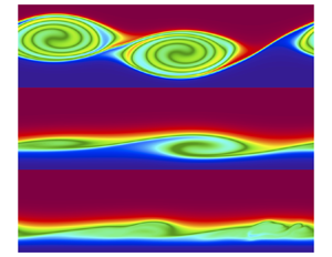
Cross-sections through  $y=0$ at various times for (a–e) shear layer far from boundary ( $d=10$, case #3), ( f–j) shear layer close to boundary ( $d=2.5$, case #1). Panels (b,g) are at their respective $t_{KH}$.

When the instability occurs near the boundary ( $d=2.5$; figure 2f–j), the evolution of the KH instability has some resemblance to the $d=10$ cases. The linear instability grows to finite amplitude (figure 2g), then 3-D secondary instabilities arise and turbulence is generated, breaking down the KH billows (figure 2h,i). Finally, the flow relaminarizes to a stable state (figure 2j). When $d=2.5$, the vertical extent of the KH billow at $t=t_{KH}$ (figure 2g) is 55 % of that for $d=10$ (figure 2b). In other words, KH billows are flatter when the shear layer is closer to the boundary. (The vertical extent of the billows is defined as the distance between two local maximum buoyancy gradients at the upper and lower edges of the billows.) This result is consistent with previous laboratory experiments (Holt Reference Holt1998). The geometrical change occurs because the impermeable boundary constrains the vertical development of the billows.
Another impact of the boundary is that the primary KH instability grows slower so the onset of turbulence is delayed. The maximum  $\mathscr {K}_{KH}$ occurs at $t_{KH}=120$ for $d=10$ (figure 2b) but is delayed to $t_{KH}=145$ for $d=2.5$ (figure 2g). A more robust demonstration of the boundary effect on the KH evolution is the dependence of $t_{KH}$ on $d$ (figure 3). When the boundary effect becomes salient, e.g. $d<4$, $t_{KH}$ increases significantly with decreasing $d$.
$d$.
Dependence of  $t_{KH}$ on $d$. Circles denote all ensemble members. Red represents the mean.

4. Pairing
In a train of KH billows, there is a range of different wavelengths including the primary KH wavelength, along with its shorter harmonics and longer subharmonics. Like all interfacial disturbances, KH instability decays exponentially and vertically away from the interface (Smyth & Carpenter Reference Smyth and Carpenter2019). The decay depth is proportional to the wavelength. Therefore, we can expect that the subharmonic mode (twice the wavelength of the fastest-growing KH mode) is influenced by the boundary most strongly because it has the greatest vertical reach. In this section, we explore the mechanisms whereby the subharmonic instability is affected by the boundary.
4.1. Energy evolution
The evolution of  $\mathscr {K}_{KH}$ and $\mathscr {K}_{sub}$ with different values of $d$ is shown in figure 4. The dependence of these energies on $d$ can be viewed as two distinct regimes. The change of $\mathscr {K}_{KH}$ and $\mathscr {K}_{sub}$ is slight when $d\geqslant 4$ (red, blue and green curves are close together), but precipitous when $d<4$ (orange, purple and yellow curves are widely separated). We interpret this to mean that boundary effects become significant when $d<4$.
Time variation of kinetic energy of the (a) primary KH and (b) subharmonic Fourier components with different values of  $d$. Each thick curve represents the average of all cases with the same $d$.
$d$.

One possible consequence of subharmonic instability is pairing, which can increase mixing significantly (Rahmani et al. Reference Rahmani, Lawrence and Seymour2014). However, pairing is found mainly in idealized simulations and laboratory experiments; it is rarely observed in geophysical flows. A possible explanation is provided by the discovery that, at high Reynolds number, pairing can be suppressed by the early emergence of a ‘zoo’ of 3-D secondary instabilities (Mashayek & Peltier Reference Mashayek and Peltier2011, Reference Mashayek and Peltier2013, Reference Mashayek and Peltier2012b). Another well-known mechanism that suppresses pairing is background stratification, which restricts vertical motion, thereby stabilizing the subharmonic mode whenever  $Ri_{0}$ exceeds approximately 3/16 (i.e. instability requires $Ri_0< k(1-k)$ and the subharmonic wavenumber is $k\simeq 1/4$, e.g. Smyth & Carpenter Reference Smyth and Carpenter2019, § 4.4). In the present simulations, we ensure that pairing is not prevented by either 3-D secondary instability or stratification by choosing $Re_0=1000$ and $Ri_0=0.12$ for all cases.
Here, we propose that the boundary can be another important factor in suppressing pairing. In the examples shown in figure 2, pairing occurs when  $d=10$ but not when $d=2.5$. To generalize the distinction, we examine the ensemble average of many cases (figure 4b and 5) over a range of $d$ values. Similar to the dependence on $Re$ (Mashayek & Peltier Reference Mashayek and Peltier2013, figure 21), we find that the maximum of $\mathscr {K}_{sub}$ decreases monotonically with decreasing $d$. Therefore, the boundary effect has similar influence on pairing to the Reynolds number effect, although the underlying mechanism is different.
Dependence of maximum subharmonic kinetic energy on  $d$. The ensemble members exhibiting laminar pairing, turbulent pairing and non-pairing are represented by blue, green and red circles, respectively, while the mean is indicated by the black line.

The spread of  $\mathscr {K}_{sub}^{max}$ tends to be larger when $d$ is large (figure 5). This is because the pairing process is sensitive to small changes in the initial conditions. Billow evolution can be categorized as laminar pairing, turbulent pairing or non-pairing (Dong et al. Reference Dong, Tedford, Rahmani and Lawrence2019; Guha & Rahmani Reference Guha and Rahmani2019; Liu et al. Reference Liu, Kaminski and Smyth2022). Laminar pairing involves the greatest amount of subharmonic kinetic energy (blue circles in figure 5), because at the time when $\mathscr {K}_{sub}$ is a maximum, turbulence has not yet grown strong enough to collapse the coherent billow structure. When the boundary effect is negligible (e.g. when $d=10$), laminar pairing occurs in a single case. Other cases with $d=10$ produce turbulent pairing (green circles), in which turbulence drains part of the kinetic energy from the emerging paired billow. When the shear layer is located close to the boundary, the maximum subharmonic kinetic energy decreases. Furthermore, more cases fail to pair (red circles). Among cases that successfully pair, most are already turbulent (turbulent pairing, green circles), while laminar pairing becomes less likely. The spread of $\mathscr {K}_{sub}^{max}$ between cases is usually smaller when $d$ is small.
One might expect that the suppression of pairing by the boundary would be accomplished via damping of the subharmonic KH instability, and such damping is in fact found for  $d<4$ (figure 6, red curve). However, a hint that the mechanism is more subtle than this is revealed by the growth rate of the primary KH mode, $\sigma _{KH}$ (figure 6, blue curve), which decreases even more than does $\sigma _{sub}$, i.e. the growth rate of the subharmonic relative to the primary increases. Based only on this comparison of growth rates, one would expect pairing to take longer but to actually be more pronounced at low $d$, contrary to figure 2. We will describe the mechanism whereby the boundary effect suppresses pairing in the following subsection.
Dependence of KH growth rate and subharmonic growth rate on  $d$ from linear stability analysis with $Ri_0=0.12$, $Re_0=1000$ and $Pr=1$.

4.2. Phase evolution
The optimal separation between the KH and subharmonic modes is
 \begin{equation} \varDelta^{KH}_{sub}\equiv\frac{x_{KH}-x_{sub}}{\lambda_{KH}}=\frac{3}{4}+n, \end{equation}
where  $n$ is an arbitrary integer, $\lambda _{KH}$ is the wavelength of the KH mode and $x_{KH}$ and $x_{sub}$ are the crest positions of the KH and subharmonic vertical velocity profiles, respectively (figure 7a). These positions are computed from the Fourier phase spectrum of the centreline vertical velocity. In this configuration, one KH billow is lifted and its neighbour is lowered by the vertical motion of the subharmonic mode (figure 7a). Thereafter, the mean shear feeds energy to the pairing billows, and a single vortex is formed (Dong et al. Reference Dong, Tedford, Rahmani and Lawrence2019; Guha & Rahmani Reference Guha and Rahmani2019). The opposite value of the optimal $\varDelta ^{KH}_{sub}$ is $1/4+n$ (figure 7b). In this case, one vortex rotates in the same direction as the subharmonic vorticity, while the other one rotates oppositely and is thus cancelled out. This process is referred to as draining (Klaassen & Peltier Reference Klaassen and Peltier1989).
Schematic of vorticity and vertical motions in terms of the subharmonic and KH modes at the onset of (a) pairing instability with optimal  $\varDelta _{sub}^{KH}=3/4$ ( $d=10,~\mathrm {case}~\#7$) and (b) draining instability with optimal $\varDelta _{sub}^{KH}=1/4$ ( $d=2.5,~\mathrm {case}~ \#2$). Buoyancy snapshots in the background of both panels demonstrate the corresponding structure. Here, $k_0$ is the subharmonic wavenumber and $x_0$ is a midway point between billows.

The evolution of  $\varDelta ^{KH}_{sub}$ (figure 8) shows that the KH and subharmonic modes require some time to lock on. The onset and end of the lock-on process are ambiguous, especially when $d$ is small. Nonetheless, the lock-on period can be qualitatively viewed as the period during which the change of $\varDelta ^{KH}_{sub}$ is the smallest (i.e. the dotted curve is most nearly horizontal). For $d=10$ (figure 8a), the lock-on value is $3/4$ from approximately $t\sim 100$ to 150 during which time pairing occurs. The highlighted red coloured case locks on to the pairing position $\varDelta _{sub}^{KH}=3/4$ relatively early, $t\sim 100$. The corresponding buoyancy field is shown in the background of figure 7(a), in which laminar pairing can be seen. In the paired state (e.g. $t=170$), when billows are replaced by a single vortex, $\varDelta _{sub}^{KH}$ switches to $1/4$. After the flow becomes turbulent, $\varDelta ^{KH}_{sub}$ fluctuates chaotically because the billows break down into turbulence, therefore $\varDelta ^{KH}_{sub}$ is not meaningful.
Time variations of  $\varDelta ^{KH}_{sub}$ with different values of $d$. Two horizontal dashed lines in each panel denote the optimal lock-on value, $\varDelta ^{KH}_{sub}=3/4$, and the opposite of optimal value, $\varDelta ^{KH}_{sub}=1/4$, respectively. Red curves indicate the cases selected in figure 7.

In cases with lower  $d$, several changes complicate the lock-on process: (i) $\varDelta ^{KH}_{sub}$ changes in time more rapidly, (ii) the time during which phase locking is sustained decreases and (iii) the value of $\varDelta ^{KH}_{sub}$ at which phase locking occurs departs from $3/4$, eventually approaching $1/4$ (figure 8b–e). For $d=6$, the lock-on value is slightly larger than $3/4$ during $t\sim 110$ to 150 (figure 8b); for $d=4$, the lock-on value is ${\sim }7/8$ during $t\sim 120\unicode{x2013}150$ (figure 8c) and, for $d=3$, the lock-on value increases to ${\sim }1$ or equivalently 0 (i.e. $x_{KH}$ and $x_{sub}$ at the same position) during $t\sim 150$ to 170 (figure 8d). When $d=2.5$ (figure 8e), the lock-on value becomes less clear because the time variation of $\varDelta ^{KH}_{sub}$ increases. Nonetheless, we can still roughly estimate the lock-on value by determining the time at which most cases converge to a similar $\varDelta ^{KH}_{sub}$ value. With this approach, a reasonable lock-on value is $1/4$ at $t\sim 170$ (figure 8e), which coincides with the optimal value for draining. The buoyancy field of the red-highlighted case, in which one vortex is enhanced while the other is suppressed, is shown in the background of figure 7(b). This result does not imply that draining always occurs when $d=2.5$; draining can often be absent depending on the details of the initial conditions (Liu et al. Reference Liu, Kaminski and Smyth2022).
It is not a coincidence that the draining lock-on value for the case  $d=2.5$ and the paired state lock-on value for the case $d=10$ (e.g. $t=150$) are both $\varDelta ^{KH}_{sub}\simeq 1/4$. This is because the pairing and draining mechanisms, though very different, both transform a pair of billows into a single vortex. When $d$ is even smaller ( $d=2$), the lock-on value and period are highly ambiguous. The boundary effect prevents the KH and subharmonic phases from locking on altogether, and therefore pairing is suppressed.
The phase difference  $\varDelta _{sub}^{KH}$ at $t=0$ exhibits substantial variability in all cases; however, this variability diminishes considerably during phase locking. This indicates that the phase-locking value is not significantly contingent upon the initial random noise. When the boundary effect is prominent, significant variability is evident between simulations from the beginning to the end.
For the small- $d$ cases (figure 8e, f), the steady, rapid increase of $\varDelta _{sub}^{KH}$ suggests an ongoing change in the phase speeds of the KH and subharmonic modes. This is confirmed by linear stability analysis (figure 9). The fastest-growing KH instability has a phase speed $c_{KH}$ while its subharmonic has half the KH wavenumber by definition, and the phase speed is $c_{sub}$. When the boundary effects are negligible ( $d=10$), both $c_{KH}$ and $c_{sub}$ are $\sim$0. However, when the shear layer is closer to the boundary, the phase speeds diverge. Therefore, $x_{KH}$ and $x_{sub}$ are constantly changing, which explains the constant change of $\varDelta ^{KH}_{sub}$ seen in figure 8(b–f). Thus, boundary proximity impedes phase locking of the KH and subharmonic modes by causing their phase speeds to diverge. In extreme cases of small $d$ (figure 8f), phase locking and pairing are prevented altogether.
Dependence of KH phase speed and subharmonic phase speed on  $d$ from linear stability analysis with $Ri_0=0.12$, $Re=1000$ and $Pr=1$.

The dependence of the phase speed difference between the KH and subharmonic modes on the parameters  $Re_0$, $Pr$ and $Ri_0$ is also of interest as a step toward a broader exploration of the parameter space. The KH instabilities change very little with increasing $Re_0$ once $Re_0$ exceeds $\sim O(10^2)$ (Smyth et al. Reference Smyth, Moum, Li and Thorpe2013); hence, we see little dependence of the phase speed difference $c_{KH}-c_{sub}$ (figure 10a). The same is true of the Prandtl number (figure 10b). There is a slight dependence on $Ri_0$ (figure 10c) when $d$ is small: the contour (thick contour) corresponding to the phase speed difference found at $Ri_0=0.12, d=4$ varies between $d=3.7$ at very low $Ri_0$ and $d=4.6$ at high $Ri_0$. Therefore the threshold $d\sim 4$ for the suppression of phase locking (and thus pairing) by boundary effects may vary only weakly with $Ri_0$. Further DNS is needed to explore the dependence of boundary effects on these parameters in the nonlinear regime.
Phase speed difference between unstable KH and subharmonic modes. A non-zero phase speed difference indicates that the KH and subharmonic modes phase lock only if forced to do so by nonlinear effects. (a) Relationship between  $d$ and $Re_0$ at a fixed value of $Ri_0=0.12$ and $Pr=1$. (b) Relationship between $d$ and $Pr$ at a fixed value of $Ri_0=0.12$ and $Re_0=1000$. (c) Relationship between $d$ and $Ri_0$ at $Re_0=1000$ and $Pr=1$. The growth rate in the shaded region of (c) is below the cutoff value, 0.001. Black contours represent phase speed difference with an interval of 0.05. Horizontal dashed lines indicate $Re_0=1000$ and $Ri_0=0.12$, respectively, in (a,c).

5. Three-dimensional secondary instabilities
Three-dimensional secondary instabilities catalyze the transition to turbulence, which in turn leads to irreversible mixing. Various 3-D secondary instabilities have been discovered; notably, the shear-aligned convective instability (Davis & Peltier Reference Davis and Peltier1979; Klaassen & Peltier Reference Klaassen and Peltier1985b) appears when KH billows become large enough to overturn the buoyancy gradient. Herein, we focus on some of the instabilities that help to explain the sources and sinks of 3-D perturbation kinetic energy in shear layers centred at different distances from the boundary. We begin by examining the case  $d=10$, where boundary effects are negligible (§ 5.1). We then examine differences that arise when $d=2.5$ (§ 5.2) and boundary effects are dominant.
5.1. The case  $d=10$: negligible boundary effects

Three-dimensional secondary instabilities grow mostly between  $t\sim 90$ and $t\sim 180$ (figure 11a, blue curve). This growth starts after the saturation of the primary KH instability, when $\langle \mathscr {K}_{2d}\rangle _{xz}$ starts to decline (red curve). Two times, indicated by the diamonds in figure 11(a), have been selected to illustrate the form of the 3-D motions in terms of the spanwise-averaged $\mathscr {K}_{3d}$. The first of these represents the early growth of $\langle \mathscr {K}_{3d}\rangle _y$ ( $t=108$, figure 11c), the second the time of most rapid growth ( $t=136$).
Negligible boundary effect when  $d=10$. (a) Time variation of 2-D and 3-D volume-averaged kinetic energy. The thick line is ensemble averaged and thin lines represent all cases. (b) Time variation of different terms of the $\sigma _{3d}$ evolution equation (2.21). All terms are ensemble averaged. Vertical dashed lines represent ensemble-averaged $t_{KH}$. For clarity in plotting, lower resolution time series have been interpolated to higher temporal resolution using cubic splines. (c,d) Show spanwise-averaged $\mathscr {K}_{3d}$ for $d=10$, case $\#3$ at $t=108$ and $t=136$, respectively. The contour lines represent spanwise-averaged buoyancy with an interval of 0.4. Note that the colour scales for (c,d) are different. Times correspond to the diamond symbols in (a,b).

The form of the 3-D motions changes because the KH billow develops different 3-D instabilities as its geometry evolves. We therefore focus on the 3-D perturbation kinetic energy evolution to explain the changes. In the early stage ( $0< t<90$), there is no 3-D instability. Growth is negative due mostly to viscous dissipation of the initial noise field.
During the earliest stage of 3-D growth, represented by time  $t=108$ (first diamond in figure 11b), 3-D motions are concentrated in the cores of the KH billows (figure 11c) and the $\mathscr {K}_{3d}$ budget is dominated by the shear production term $\mathscr {R}_{3d}$ (figure 11b). This is because the spanwise vortex tube at the core of each billow is distorted sinusoidally. Spanwise vorticity is thus redirected towards the $x$–
$x$– $z$ plane such that the Reynolds stress $\langle u_{3d}w_{3d}\rangle _{xyz}$ becomes negative (as illustrated in Smyth Reference Smyth2006, figure 8). This 3-D stress field works with the mean shear ${\rm d}\bar {U}/{\rm d}z$ to produce 3-D kinetic energy. Since ${\rm d}\bar {U}/{\rm d}z$ is large near the billow core, the shear production quantified by $\mathscr {R}_{3d}$ is dominant. This 3-D secondary instability exhibits similar characteristics to the central-core mode found in Klaassen & Peltier (Reference Klaassen and Peltier1991), hence we identify it as central-core instability (CCI).
During the maximum growth stage ( $t=136$, second diamond in figure 11b), 3-D motions in the central core are no longer dominant as $\langle \mathscr {K}_{3d}\rangle _y$ is mainly concentrated at the margins of the billows (figure 11d). At this stage, the primary KH billows roll up. This results in regions of statically unstable buoyancy variation within and surrounding the billow cores. The buoyancy production $\mathscr {H}_{3d}$ becomes the dominant energy source while $\mathscr {A}_{3d}$ and $\mathscr{S}h_{3d}$ also increase. This is all consistent with the emergence of shear-aligned convection rolls via the secondary convective instability (SCI; Klaassen & Peltier Reference Klaassen and Peltier1985a). Vorticity is created when vortex tubes are stretched and is exchanged between different components when vortex tubes bend and tilt. The 2-D velocity gradients increase along with the stretching and bending of vortex tubes surrounding the billows, the stretching deformation term, $\mathscr {A}_{3d}$, and the shear deformation term, $\mathscr{S}h_{3d}$, both increase.
Beyond the time when  $\sigma _{3d}$ is a maximum, the billows start to pair at $t\sim 150$, and $\mathscr {R}_{3d}$ regains its dominance over the other terms. The shear-aligned convection rolls are still active at the periphery of the billow core, but gradually break down into turbulence; therefore $\mathscr {H}_{3d}$ declines toward zero. After the pairs of billows have amalgamated, the extraction of 3-D perturbation kinetic energy from the background mean shear decreases. During the post-turbulent stage, all terms gradually decay.
The fact that the evolution of  $\mathscr {R}_{3d}$ when boundary effects are negligible includes two local maxima is consistent with the findings of Mashayek & Peltier (Reference Mashayek and Peltier2013). However, they found that, prior to billow saturation, buoyancy production is the major source term while we found that $\mathscr {R}_{3d}$ is dominant. The difference may be due to a difference in the initial random noise field – Mashayek & Peltier (Reference Mashayek and Peltier2013) applied noise to both the buoyancy and velocity fields whereas we perturbed only the velocity.
5.2. The case $d=2.5$: strong boundary effects

When the boundary effect is strong (e.g.  $d=2.5$), growth rates of both $\langle \mathscr {K}_{2d}\rangle _{xz}$ and $\langle \mathscr {K}_{3d}\rangle _{xyz}$ are reduced relative to cases with negligible boundary effects (compare figures 11a and 12a), as are their maximum values.
Similar to figure 11 but with the case  $d=2.5$. Case $\#1$ is selected for (c,d).

At maximum growth ( $t=176$, figure 12d), there are neither clear unstable sublayers nor 3-D motions in layers surrounding the billows. Instead, $\langle \mathscr {K}_{3d}\rangle _y$ remains concentrated in the core, suggesting that SCI is suppressed. A conspicuous impact of the boundary is that $\mathscr {R}_{3d}$ dominates all other source terms from the initial-growth stage of the instability to the post-turbulent stage (figure 12b), rather than being supplanted by $\mathscr {H}_{3d}$ as the primary billows roll up (cf. § 5.1). The terms $\mathscr {H}_{3d}$ (red line in figure 12b), $\mathscr {A}_{3d}$ and $\mathscr{S}h_{3d}$ are small throughout the evolution because the overturning within the billow is suppressed by the boundary. This suggests that the balance is mostly between the energy extraction from the background mean shear and the viscous dissipation of the 3-D perturbations.
We conclude that three-dimensionalization is via CCI alone when the boundary effect is strong (figure 12c,d).
5.3. Effects of boundary proximity on SCI
We have seen that, for the single case  $d=2.5$, the main effect of the boundary on 3-D instabilities is the suppression of SCI. The Rayleigh number provides a compact metric for SCI that we can examine as a function of $d$, thus gaining a more comprehensive view of the boundary proximity effect. We define the Rayleigh number at $t_{KH}$ for the statically unstable regions (Klaassen & Peltier Reference Klaassen and Peltier1985b) as
 \begin{equation} Ra={-}Re^2Ri_0Pr\frac{\partial \bar{b}}{\partial z}\delta^4, \end{equation}
where  ${\partial \bar {b}}/{\partial z}$ is the average buoyancy gradient across the most unstable layer, and $\delta$ is its dimensionless thickness. The critical $Ra$ for convective instability in a layer with free-slip upper and lower boundaries, an approximation to the superadiabatic regions found here, is $Ra_c \approx 657.5$ (e.g. Smyth & Carpenter Reference Smyth and Carpenter2019).
When  $d\geqslant 4$ (figure 13), $Ra$ is more than 1 order of magnitude larger than $Ra_c$, suggesting that SCI is prominent. A precipitous drop in $Ra$ can be seen when $d<4$, indicating that the boundary suppresses SCI (as seen in figure 12).
Dependence of Rayleigh number on  $d$ at $t_{KH}$. Circle symbols are all ensemble cases and red dots indicate the mean of the ensembles. Horizontal line denotes the critical Rayleigh number $Ra_c$, and has a value of 657.5.

Most cases for  $d=2$ fail to satisfy the criterion $Ra>Ra_c$, and as a result, convective motions are suppressed within the KH billow.
5.4. Timing of subharmonic and 3-D secondary instabilities
The timing of the turbulence emergence relative to the subharmonic instability is critical to pairing (Mashayek & Peltier Reference Mashayek and Peltier2013; Liu et al. Reference Liu, Kaminski and Smyth2022) and therefore to mixing. Thus,  $t_{sub}$ and $t_{3d}$ are useful measures for understanding the competition between the subharmonic and 3-D secondary instabilities. The difference between $t_{3d}$ and $t_{sub}$ tends to decrease as $d$ decreases (figure 14a). This suggests that the subharmonic instability is more susceptible to interference by turbulence when the boundary effect is strong. (The slope of the mean $t_{3d}-t_{sub}$ vs $d$ is reversed between $d=2.5$ and $d=3$, but the reversal is not statistically significant.)
(a) Dependence of time difference between  $t_{3d}$ and $t_{sub}$ on $d$. (b) Dependence of $t_{3d}$ and $t_{sub}$ on $d$. Circles are all ensemble cases. Data points represent the ensemble mean. The deviated cases of $d=2$ are not shown in the figure.

To identify the source of this behaviour, we next focus on  $t_{sub}$ and $t_{3d}$ individually (figure 14b). A monotonic increase of $t_{sub}$ with decreasing $d$ can be seen (figure 14b); the increase becomes more pronounced when $d<4$. Thus, $\mathscr {K}_{sub}$ requires more time to reach to its maximum when the boundary effect is greater. The increase of $t_{sub}$ is owing to the fact that phase lock between the KH and subharmonic modes is prevented due to the divergence of the corresponding phase speeds (§ 4).
The increase of  $t_{3d}$ with decreasing $d$ when $d<4$ is due to suppression of 3-D secondary instabilities by the boundary, as has been demonstrated in § 5.2. Even though $t_{sub}$ increases considerably at $d=2$ and $d=2.5$, 3-D secondary instabilities (and hence the onset of turbulence) are also delayed. Therefore, subharmonic instability may arise at $d=2.5$ because turbulence emerges too late to overtake it. When $d=2$, the subharmonic does not reach maximum amplitude until after 3-D secondary instabilities have already appeared.
6. Turbulent mixing
In the latter part of each simulation, the flow consists of slowly decaying sheared turbulence. The energy in the 3-D motions is supported mainly by shear production (figures 11b and 12b, blue curves) and diminished by viscosity (purple curves). We now discuss the energy budget of this turbulence in the context of irreversible mixing. The instantaneous mixing efficiency has been calculated using (2.18) and is shown in figure 15(c), as are the irreversible mixing rate (figure 15a) and the total dissipation rate (figure 15b) for various boundary proximity values. Initially, a large dissipation rate arises due mainly to the viscous decay of the random noise. Dissipation rapidly decreases to a near-constant (although non-zero) value as the mean flow continues to diffuse (figure 15b), while the mixing rate is near zero.
Time variation of (a) mixing rate, (b) total dissipation rate and (c) instantaneous mixing efficiency with different values of  $d$. Horizontal line denotes the canonical value of $\eta _i\sim 1/6$. Time variation of changes from the initial state in (d) available potential energy $\mathscr {P}_a$, (e) background potential energy $\mathscr {P}_b$ associated with macroscopic motions. Volume-averaged ( f) 2-D kinetic energy $\mathscr {K}_{2d}$, (g) 3-D kinetic energy $\mathscr {K}_{3d}$. (h) Turbulent diffusivity, $K_{\rho }$. All curves are ensemble averaged.

For all  $d$, the instantaneous mixing rate $\mathscr {M}$ and mixing efficiency exhibit two peaks (figure 15a,c). The first peak of $\mathscr {M}$ and $\eta _i$ (e.g. at $t\sim 130$, $d=10$) is associated with the roll up of the KH billows. Because they are not yet turbulent, the KH billows develop strong buoyancy gradients where $\mathscr {M}$ is large. During this time, $\mathscr {P}_a$ is rapidly converted to background potential energy $\mathscr {P}_b$ (figure 15d,e). The dissipation rate is smaller than the mixing rate because the flow is not turbulent at this stage; hence the irreversible mixing efficiency $\eta _i$ is greatest.
When the shear layer is close to the boundary (small  $d$), the roll-up of the KH billows weakens, and SCI (§ 5.2) is therefore suppressed. Because of this, the first peak of $\mathscr {M}$ (e.g. red curve at $t=140$ when $d=3$ in figure 15a) is reduced. Boundary proximity also reduces dissipation during this time (figure 15b).
A precipitous drop in  $\eta _i$ occurs immediately after the first local maximum (figure 15c), due to the emergence of the 3-D secondary instabilities that collapse the KH billows. The value of $\langle \mathscr {K}_{3d}\rangle _{xyz}$ rapidly increases at this stage, e.g. $t\sim 140\unicode{x2013}160$ for $d=10$ (figure 15g), suggesting the emergence of 3-D turbulence. Therefore, $\mathscr {P}_a$ (figure 15d) as well as $\langle \mathscr {K}_{2d}\rangle _{xz}$ (figure 15f) drop to a local minimum because the 2-D KH billow structure is partly destroyed. As a consequence, the instantaneous mixing efficiency decreases as $\mathscr {M}$ is reduced but $\epsilon$ simultaneously increases.
The second peak of  $\mathscr {M}$ and $\eta _i$ (e.g. at $t\sim 200$ for $d=10$ in figure 15a) is associated with the turbulent stage of the flow evolution. The dissipation rate (figure 15b) reaches its maximum shortly after the maximum of $\mathscr {M}$. Pairing involves significant vertical motion and thus enhances $\mathscr {P}_a$ (e.g. $t=150\unicode{x2013}180$ when $d=10$ in figure 15d). Therefore, $\mathscr {P}_b$ and $\mathscr {M}$ both increase at $t=180$. In contrast, the suppression of pairing by the boundary effect (e.g. $t=200$ when $d=3$ in figure 15d) reduces $\mathscr {P}_a$ as well as $\mathscr {P}_b$. As a result, mixing efficiency is reduced.
During the fully turbulent stage, the instantaneous mixing efficiency roughly converges to the canonical value of  $\eta _i\sim 1/6$ or $\varGamma =0.2$. In the post-turbulent stage, $\mathscr {M}$ drops to $\sim$0 whereas the mean kinetic energy continues to dissipate. Therefore, $\eta _i$ gradually decays to $\sim$0.
We further relate the mixing efficiency to a turbulent diffusivity associated with irreversible mixing devised by Salehipour & Peltier (Reference Salehipour and Peltier2015, their (2.23)). Using the present non-dimensionalization, this is
 \begin{equation} K_\rho=\varGamma\frac{Re_b}{Re_0}, \end{equation}
where  $Re_b$ is the buoyancy Reynolds number $\epsilon ^*/\nu ^* N^{*2}$. The time variation of $K_\rho$ is shown in figure 15(h) with different values of $d$. The first peak of $K_\rho$ is associated with the roll up of the KH billow, during which the mixing efficiency is maximum. The second peak is associated with turbulence, where $\epsilon$ and $\langle \mathscr {K}_{3d}\rangle _{xyz}$ are large. The value of $K_\rho$ drops significantly with decreasing $d$ as does the mixing rate.
We further demonstrate the importance of the route to turbulent mixing by showing the cumulative mixing, dissipation and mixing efficiency (2.19) for various values of  $d$ in figure 16. All three quantities decrease monotonically with decreasing $d$. The net mixing and dissipation vary slightly when $d\geqslant 4$, but drop sharply as $d<4$ (figure 16a,b). This suggests that the impact of the boundary on mixing and dissipation becomes prominent when $d$ is less than 4 due to the suppression of pairing and SCI. The abrupt decrease in cumulative mixing efficiency observed at $d<4$ could be attributed to a combination of changes in net dissipation and mixing. We consider the derivative of the cumulative mixing efficiency with respect to $d$
$d$
 \begin{equation} \frac{1}{\eta_c}\frac{\partial\eta_c}{\partial d}=\frac{1}{\varGamma_c+1}\left(\frac{1}{\mathscr{M}_c}\frac{\partial\mathscr{M}_c}{\partial d}-\frac{1}{\epsilon_c}\frac{\partial\epsilon_c}{\partial d}\right), \end{equation}
where the subscript ‘c’ refers to cumulative values. The boundary effect diminishes net dissipation (figure 16a, dotted line), leading to an increase in cumulative mixing efficiency ((6.2), second term in parentheses). However, it also diminishes net mixing, which is a key factor contributing to the sharp reduction in cumulative mixing efficiency when  $d$ is less than 4. Because the relative change in $\mathscr {M}_c$ is considerably greater than that in $\epsilon _c$, i.e. $({1}/{\mathscr {M}_c})({\partial \mathscr {M}_c}/{\partial d})>({1}/{\epsilon _c})({\partial \epsilon _c}/{\partial d})$, the change in $\eta _c$ is particularly pronounced.
Cumulative (a) mixing (solid line) and dissipation (dotted line), and (b) mixing efficiencies calculated over an entire mixing event for different values of  $d$. Error bars are standard error of the mean.

For smaller  $d$, e.g. $d=2$, the net mixing $\int \mathscr {M} \,{\rm d}t$ is small, but the net dissipation persists since the dissipation of the mean flow is non-zero. Therefore, the efficiency of mixing is considerably reduced.
7. Summary and discussion
In geophysical flows, much of the most important shear-driven turbulent mixing appears near boundaries. Here, we have shown that boundary proximity significantly modifies the life cycle of turbulence in a stably stratified shear layer. A classical KH instability has been investigated by performing ensembles of DNS experiments with  $Re_0=1000$, $Ri_0=0.12$ and $Pr=1$. Absent boundary effects, the moderately low $Ri_0$ and $Re_0$ ensure the amalgamation of the KH billows. Our study describes the impact of boundary proximity on the primary KH instability, the subharmonic pairing instability, the 3-D secondary instability and the resulting turbulent mixing.
When the shear layer is close to the boundary, the primary KH billows are geometrically flatter. Furthermore, the evolution of the KH instability is extended over longer periods of time, so the transition to turbulence is delayed.
Mashayek & Peltier (Reference Mashayek and Peltier2013) explained that when  $Re_0$ is sufficiently large, the early emerging 3-D secondary instabilities can suppress pairing. Pairing would also be suppressed by gravity at higher $Ri_0$ (Smyth Reference Smyth2003; Mashayek & Peltier Reference Mashayek and Peltier2012a), and tends to be either unchanged or suppressed with an increase in $Pr$ (Salehipour et al. Reference Salehipour, Peltier and Mashayek2015; Rahmani, Seymour & Lawrence Reference Rahmani, Seymour and Lawrence2016). Our study provides an additional explanation as to why pairing is rarely observed in geophysical flows. When the boundary effect is negligible, the linear phase speeds of the KH and subharmonic modes are virtually identical and equal to zero. When the shear layer is close to the boundary, on the other hand, the KH and subharmonic phase speeds diverge so that phase locking is prevented and pairing is therefore suppressed.
During the time when the primary KH instability is growing exponentially, CCI triggers 3-D motions in the cores of the billows. This is because the vortex at the central core tilts, resulting in energy extraction from the background shear via Reynolds stress. At this stage, CCI dominates for all boundary proximities.
When the boundary effect is negligible, SCI becomes the dominant 3-D secondary instability. The buoyancy production is greatly enhanced because unstable sublayers are formed within the billows. The boundary effect suppresses SCI because the roll up of the billows is counteracted by bottom drag. In contrast to the suppression of SCI, CCI remains dominant throughout the preturbulent stage. By forcing an alternate route for the transition of a 2- KH billow to 3-D turbulence, the boundary effect inevitably changes the resulting mixing.
The suppression of pairing weakens the conversion from  $\mathscr {P}_a$ to $\mathscr {P}_b$ and reduces irreversible mixing. Although the suppression of pairing leads to a decline in dissipation, it is likely that dissipation near the boundary is amplified when $d$ is smaller. Therefore, instantaneous mixing efficiency is reduced. Furthermore, the suppression of SCI by the boundary also diminishes the mixing rate and mixing efficiency. The cumulative irreversible mixing, dissipation and mixing efficiency, as well as turbulent diffusivity, decrease monotonically with decreasing distance from the shear layer to the boundary.
This study has been confined to a small subset of the continuum of initial states for practical reasons. Experiments with large  $Re_0$ and $Pr$ are expected to be affected by the boundary but the effect may manifest differently because the route to turbulent mixing is inherently different. Both the threshold value for $d$ at which boundary effects become strong and the onset time of 3-D secondary instability are expected to be sensitive to the value of the Reynolds number. As mentioned in § 4, Mashayek & Peltier (Reference Mashayek and Peltier2013) show that 3-D secondary instability grows more rapidly when $Re_0$ is large, therefore, $t_{3d}$ is expected to be smaller and pairing is, therefore, less likely. The effects of increasing $Re_0$ on $t_{sub}$ and on the threshold value of $d$ are subjects for future study.
The cores of the KH billows are referred to as ‘quiet’ in observations of the high- $Re_0$ and high- $Pr$ flow of a salt-stratified estuary by Geyer et al. (Reference Geyer, Lavery, Scully and Trowbridge2010). The DNS experiments have shown that, with large $Re_0$ and $Pr$, there is no density variance in the core of the billows but only in the periphery and the braid (Salehipour et al. Reference Salehipour, Peltier and Mashayek2015). This is potentially because the core of the billows is already well mixed due to previous 3-D secondary instability. In contrast, our results show that pairing and CCI play an important role during the evolution of the KH instability and the resulting mixing. A comprehensive understanding of the boundary effects on shear instability and the resulting turbulent mixing, particularly in the geophysical cases, will require the exploration of large $Re_0$ and $Pr$ cases.
We have considered a classical KH instability to understand the boundary proximity effect. However, KH is not the only instability that may arise in a stratified shear flow. When buoyancy gradients are sufficiently sharp, the flow may be susceptible to the Holmboe instability (Holmboe Reference Holmboe1962). Furthermore, flows with asymmetric background profiles may exhibit instabilities with a mixture of KH- and Holmboe-like behaviour (e.g. Carpenter, Lawrence & Smyth Reference Carpenter, Lawrence and Smyth2007; Yang, Tedford & Lawrence Reference Yang, Tedford and Lawrence2019; Olsthoorn, Kaminski & Robb Reference Olsthoorn, Kaminski and Robb2023). Understanding how boundary proximity affects these processes may provide insights on future parameterizations of mixing in the ocean near boundaries. Studying beyond shear-driven turbulence and whether the alternative mechanisms have similar mixing properties may also be of future interest.
We note that the flow profiles considered here differ from real-world boundary layer flows in two key ways. The first is our choice of a hyperbolic–tangent shear and stratification. Classical turbulent boundary layer flows often exhibit logarithmic profiles with elevated shear at the boundary (e.g. Marusic et al. Reference Marusic, Monty, Hultmark and Smits2013; Bluteau et al. Reference Bluteau, Ivey, Donis and McGinnis2018), although the specific details of the flow vary with surface roughness, ambient stratification and external pressure gradients. While the profiles considered here differ from these classical boundary layers, we make this choice so as to facilitate comparison between our simulations and the isolated hyperbolic–tangent shear layer commonly studied in the KH literature. Secondly, the bottom boundary layer or the surface layer in the ocean is often turbulent. While the effect of boundary proximity on KH instability is pronounced, pre-existing turbulence should be taken into account for KH instabilities (Brucker & Sarkar Reference Brucker and Sarkar2007; Kaminski & Smyth Reference Kaminski and Smyth2019), especially near boundaries, where mixed layers are not initially laminar.
The flat bottom boundary is a simplification, as the real-world topography can be much more complex. Shear instability may occur near a ridge or a sloping topography. Internal waves may be generated near those boundaries, where the base flow may be altered and the boundary effect is not uniform. A nearby surface boundary, e.g. where the shear is created by wind stress in a diurnal warm layer (Hughes et al. Reference Hughes, Moum, Shroyer and Smyth2021), can similarly reduce the growth rate of the instability. However, the frictional effect on the shear instability is smaller at the surface than at the bottom, as represented in our model by the free-slip top boundary (§ 2.1). We have shown that SCI is suppressed by a no-slip boundary because the boundary drag counteracts the roll up of the billows. Nonetheless, the no-slip condition results in higher dissipation near the boundary, potentially altering the evolution of the billows (Baglaenko Reference Baglaenko2016). With a free-slip boundary, however, no drag counteracts the roll-up process. Therefore, the suppression of SCI due to the free-slip boundary is expected to be smaller. The effects of different boundary types (e.g. free slip, free surface) should be a focus for future research.
This study can potentially provide insights into future measurements near boundaries in the atmosphere and oceans. The dependence of mixing efficiency on boundary proximity can be estimated via microstructure measurements. Furthermore, acoustic backscatter measurements can delineate how the geometry of the KH billows varies with boundary proximity (e.g. Holleman et al. Reference Holleman, Geyer and Ralston2016; Tu et al. Reference Tu, Fan, Lian, Liu, Liu, Kaminski and Smyth2020).
While pairing is rarely detected in geophysical flows, the related phenomena called ‘tubes’ and ‘knots’ are commonly observed in the atmosphere (Thorpe Reference Thorpe2002; Smyth & Moum Reference Smyth and Moum2012; Fritts et al. Reference Fritts, Wang, Lund and Thorpe2022). Tubes and knots arise when KH billow cores are misaligned. Unlike pairing in our study, knots often appear locally in the spanwise direction. Fritts et al. (Reference Fritts, Wang, Lund and Thorpe2022) has found that the transition to turbulence is accelerated and turbulence is significantly stronger in tubes and knots than in other types of secondary instabilities (e.g. SCI). Future studies should address the effects of boundary proximity on tubes and knots. In particular, the question of whether boundary proximity suppresses tubes and knots by reducing the misalignment of the KH billow cores will be of interest.
Acknowledgements
This paper is part of the first author's PhD thesis at Oregon State University. We appreciate useful input from advisory committee members J. Moum, J. Liburdy, J. Nash and B. Pearson. We appreciate J. Taylor's work in creating and curating DIABLO. We acknowledge high-performance computing support on Cheyenne (doi:10.5065/D6RX99HX) provided by NCAR's Computational and Information Systems Laboratory, sponsored by the US National Science Foundation.
Funding
This work was funded by the US National Science Foundation under grant OCE-1830071. A.K.K. was supported as the Ho-Shang and Mei-Li Lee Faculty Fellow in Mechanical Engineering at UC Berkeley.
Declaration of interests
The authors report no conflict of interest.
Data availability statement
DIABLO is available at https://github.com/johnryantaylor/DIABLO. Output data are available by request to the authors.


 Open access