







1. Introduction and main results
This article is concerned with the Cauchy problem for fourth-order Schrödinger equation involving second-order nonlinear derivative term
 \begin{eqnarray} \left \{\begin{array}{lr} iu_{t}-\Delta ^2u+u\Delta |u|^2+|u|^{p-1}u=0,\,\,t\geq 0,\,\,x\in \mathbb{R}^{N},\\ u(0,x)=u_{0}(x),\,\,\,\,\,x\in \mathbb{R}^{N},\\ \end{array}\right . \end{eqnarray}
where $i^2=-1, u(t,x)\,:\,\mathbb{R}_{+}\times \mathbb{R}^{N}\to \mathbb{C}$
is a complex-valued function, and
$i^2=-1, u(t,x)\,:\,\mathbb{R}_{+}\times \mathbb{R}^{N}\to \mathbb{C}$
is a complex-valued function, and $u\Delta |u|^2$
is the second-order nonlinear derivative term, in which the power exponent
$u\Delta |u|^2$
is the second-order nonlinear derivative term, in which the power exponent $p$
satisfies
$p$
satisfies
 \begin{eqnarray} \left \{\begin{array}{l@{\quad}l}1\lt p\lt +\infty , & \text{when} \,2\lt N\leq 4,\\[3pt] 1\lt p\lt \frac {N+4}{N-4}, & \text{when}\,4\lt N\leq 6,\\[3pt] 1\lt p\lt \frac {3N+2}{N-2},& \text{when}\,N\gt 6.\end{array}\right . \end{eqnarray}
Eq. (1.1) is a significant fourth-order Schrödinger equation with second-order derivative-type nonlinearity that serves as a fundamental model in diverse fields, including plasma physics, fluid mechanics, the theory of Heisenberg ferromagnets and magnons and dissipative quantum mechanics [Reference Hasse1–Reference Yu and Shukla3]. Moreover, this equation is highly appealing due to its close connections with numerous renowned and significant physical models. For instance, if one omits the nonlinear derivative term from Eq. (1.1), then it becomes the classical fourth-order Schrödinger equation
 \begin{equation} iu_t + \Delta ^2 u + \lambda |u|^p u = 0, \quad t\geq 0,\,\,x\in \mathbb{R}^{N}, \end{equation}
which has emerged as a focal point for many researchers in the past few years. In the focusing case $\lambda \lt 0$
and the power exponent
$\lambda \lt 0$
and the power exponent $p = \frac {8}{N - 4}$
with
$p = \frac {8}{N - 4}$
with $N \geq 5$
, Miao, Xu and Zhao [Reference Miao, Xu and Zhao4] established the global existence of solutions to (1.3) and then exhibited the scattering behaviour under radial symmetry assumptions. For the defocusing case
$N \geq 5$
, Miao, Xu and Zhao [Reference Miao, Xu and Zhao4] established the global existence of solutions to (1.3) and then exhibited the scattering behaviour under radial symmetry assumptions. For the defocusing case $\lambda \gt 0$
and the power exponent
$\lambda \gt 0$
and the power exponent $2 \lt p \leq \frac {2N}{N - 4}$
with
$2 \lt p \leq \frac {2N}{N - 4}$
with $N \geq 5$
, Pausader [Reference Pausader5] analysed the global well-posedness and scattering property under radially symmetric initial data. In [Reference Pausader6], Pausader devoted to the cubic defocusing fourth-order Schrödinger equation (i.e.,
$N \geq 5$
, Pausader [Reference Pausader5] analysed the global well-posedness and scattering property under radially symmetric initial data. In [Reference Pausader6], Pausader devoted to the cubic defocusing fourth-order Schrödinger equation (i.e., $\lambda \gt 0$
and
$\lambda \gt 0$
and $p = 2$
); he showed that the solutions are globally well-posed for space dimensions
$p = 2$
); he showed that the solutions are globally well-posed for space dimensions $N \leq 8$
and exhibited the scattering behaviour at
$N \leq 8$
and exhibited the scattering behaviour at $5 \leq N \leq 8$
. Later, Miao, Wu and Zhang [Reference Miao, Wu and Zhang7] further extended the range of the dimension of interaction Morawetz estimate of [Reference Pausader6] and thereby investigated the global well-posedness and scattering theory for (1.3) in
$5 \leq N \leq 8$
. Later, Miao, Wu and Zhang [Reference Miao, Wu and Zhang7] further extended the range of the dimension of interaction Morawetz estimate of [Reference Pausader6] and thereby investigated the global well-posedness and scattering theory for (1.3) in $H^s(\mathbb{R}^N)$
, where
$H^s(\mathbb{R}^N)$
, where $\lambda \gt 0$
,
$\lambda \gt 0$
, $p = 2$
,
$p = 2$
, $0 \lt s \lt 2$
and
$0 \lt s \lt 2$
and $5 \leq N \lt 7$
.
$5 \leq N \lt 7$
.
In [Reference Zhu, Zhang and Yang8], Zhu, Zhang and Yang considered the following fourth-order nonlinear Schrödinger equation
 \begin{equation} i u_t - \Delta ^2 u + |u|^p u = 0, \quad \,\,t\geq 0,\,\,x\in \mathbb{R}^{N}, \end{equation}
and explored the limiting behaviour of blow-up solutions in the Sobolev space $H^2(\mathbb{R}^N)$
for power exponent
$H^2(\mathbb{R}^N)$
for power exponent $p = \frac {8}{N}$
. Later, Zhu, Zhang and Yang [Reference Zhu, Zhang and Yang9] further proved the existence of nontrivial solutions through the method of profile decomposition of bounded sequences in
$p = \frac {8}{N}$
. Later, Zhu, Zhang and Yang [Reference Zhu, Zhang and Yang9] further proved the existence of nontrivial solutions through the method of profile decomposition of bounded sequences in $H^2(\mathbb{R}^N)$
for a power exponent
$H^2(\mathbb{R}^N)$
for a power exponent $\frac {8}{N} \lt p \lt \frac {2N}{(N-4)^+}$
, where
$\frac {8}{N} \lt p \lt \frac {2N}{(N-4)^+}$
, where $\frac {2N}{(N-4)^+}$
equals
$\frac {2N}{(N-4)^+}$
equals $+\infty$
for
$+\infty$
for $N \leq 4$
and equals
$N \leq 4$
and equals $\frac {2N}{N-4}$
for
$\frac {2N}{N-4}$
for $N \geq 5$
. Dinh [Reference Dinh10] constructed a profile decomposition for bounded sequences in the intersection space
$N \geq 5$
. Dinh [Reference Dinh10] constructed a profile decomposition for bounded sequences in the intersection space $\dot {H}^{\gamma _c} \cap \dot {H}^2$
; he studied the blow-up concentration phenomena and the limiting profile of blow-up solutions in
$\dot {H}^{\gamma _c} \cap \dot {H}^2$
; he studied the blow-up concentration phenomena and the limiting profile of blow-up solutions in $\dot {H}^{\gamma _c}$
-norm, where
$\dot {H}^{\gamma _c}$
-norm, where $\gamma _c = \frac {Np - 8}{2p}$
and
$\gamma _c = \frac {Np - 8}{2p}$
and $\frac {8}{N} \lt p \lt \frac {8}{(N-4)^+}$
(note that
$\frac {8}{N} \lt p \lt \frac {8}{(N-4)^+}$
(note that $\frac {8}{(N-4)^+}$
equals
$\frac {8}{(N-4)^+}$
equals $+\infty$
for
$+\infty$
for $N \leq 4$
and equals
$N \leq 4$
and equals $\frac {8}{N - 4}$
for
$\frac {8}{N - 4}$
for $N \geq 5$
).
$N \geq 5$
).
In [Reference Miao and Zhang11], Miao and Zhang analysed the following nonlinear Schrödinger-type equation:
 \begin{equation} i u_t + ({-}\Delta )^m u = f(u), \quad \,\,t\geq 0,\,\,x\in \mathbb{R}^{N}, \end{equation}
where $m \geq 1$
is a positive integer,
$m \geq 1$
is a positive integer, $f(z) = \partial V(z)/\partial \bar {z} \in C(\mathbb{C}, \mathbb{C})$
and
$f(z) = \partial V(z)/\partial \bar {z} \in C(\mathbb{C}, \mathbb{C})$
and $V(z) \in C^1(\mathbb{C}, \mathbb{R}^+)$
; they established the global well-posedness in
$V(z) \in C^1(\mathbb{C}, \mathbb{R}^+)$
; they established the global well-posedness in $H^m$
-norm by deriving Strichartz-type estimates for its linearized problem, along with nonlinear estimates in the Besov spaces. In the mixed power nonlinearities,
$H^m$
-norm by deriving Strichartz-type estimates for its linearized problem, along with nonlinear estimates in the Besov spaces. In the mixed power nonlinearities, $f(u) = \lambda _1 |u|^{p_1} u + \lambda _2 |u|^{p_2} u$
, Guo and Wang [Reference Guo and Wang12] discussed the existence and scattering to (1.5) in
$f(u) = \lambda _1 |u|^{p_1} u + \lambda _2 |u|^{p_2} u$
, Guo and Wang [Reference Guo and Wang12] discussed the existence and scattering to (1.5) in $H^s$
-norm under the assumption of small initial data, where the critical regularities are defined by
$H^s$
-norm under the assumption of small initial data, where the critical regularities are defined by $s(p_i) = \frac {N}{2} - \frac {2m}{p_i}$
, with the range
$s(p_i) = \frac {N}{2} - \frac {2m}{p_i}$
, with the range $s(p_1) \leq s \leq s(p_2)$
. For more results involving the qualitative properties of nonlinear Schrödinger equations with mixed power nonlinearities, we refer readers to see [Reference Zhang and Zheng13, Reference Xu and Xu14] and the references therein.
$s(p_1) \leq s \leq s(p_2)$
. For more results involving the qualitative properties of nonlinear Schrödinger equations with mixed power nonlinearities, we refer readers to see [Reference Zhang and Zheng13, Reference Xu and Xu14] and the references therein.
In [Reference Segata15], Segata investigated the fourth-order nonlinear Schrödinger-type equation
 \begin{equation} i u_t + \partial _x^2 u + \nu \partial _x^4 u = F\big(u, \bar {u}, \partial _x u, \partial _x \bar {u}, \partial _x^2 u, \partial _x^2 \bar {u}\big), \quad x, t \in \mathbb{R}, \end{equation}
and then established the local well-posedness of solutions, where the nonlinearity $F$
includes the first-order and second-order derivative terms. Note that this equation, originally introduced by Fukumoto and Moffatt [Reference Fukumoto and Moffatt16], governs the three-dimensional dynamics of an isolated vortex filament within an inviscid, incompressible fluid that occupies an unbounded spatial region. Building upon previous work, Huo and Jia [Reference Huo and Jia17] refined the results of [Reference Segata15] for the above equation by relaxing the required conditions.
$F$
includes the first-order and second-order derivative terms. Note that this equation, originally introduced by Fukumoto and Moffatt [Reference Fukumoto and Moffatt16], governs the three-dimensional dynamics of an isolated vortex filament within an inviscid, incompressible fluid that occupies an unbounded spatial region. Building upon previous work, Huo and Jia [Reference Huo and Jia17] refined the results of [Reference Segata15] for the above equation by relaxing the required conditions.
To the best of the authors’ knowledge, several studies have been conducted on the qualitative analysis (such as the existence and stability of solutions) of second-order Schrödinger equations featuring second-order derivative-type nonlinearity. These models have garnered considerable attention due to their fundamental role in describing diverse physical phenomena across various scientific fields. For example, Colin [Reference Colin18] studied the following second-order nonlinear derivative-type Schrödinger equation
 \begin{equation} i u_t + \Delta u + u \Delta (|u|^2) + |u|^p u = 0, \quad \,\,t\geq 0,\,\,x\in \mathbb{R}^{N}, \end{equation}
and proved the local well-posedness at arbitrary space dimension $N \geq 1$
, without requiring smallness conditions on the initial data. Chen, Li and Wang [Reference Chen, Li and Wang19] gave the proof of stability and instability of standing wave solutions under certain conditions
$N \geq 1$
, without requiring smallness conditions on the initial data. Chen, Li and Wang [Reference Chen, Li and Wang19] gave the proof of stability and instability of standing wave solutions under certain conditions $p$
and
$p$
and $N$
. Chen and Guo [Reference Chen and Guo20] showed the finite time blow up of solutions when the initial energy is positive and gave the strong instability in
$N$
. Chen and Guo [Reference Chen and Guo20] showed the finite time blow up of solutions when the initial energy is positive and gave the strong instability in $H^1(\mathbb{R})$
-norm for its standing wave solutions at space dimension
$H^1(\mathbb{R})$
-norm for its standing wave solutions at space dimension $N = 1$
. For the case
$N = 1$
. For the case $p = 2$
, Shu and Zhang [Reference Shu and Zhang21] derived a sharp condition that separates the global existence from blow-up by using the potential well method and concavity argument. Xu et al. [Reference Xu and Xu22] further gave the sharp condition of blow-up and global existence through the potential well theory and concavity method, where
$p = 2$
, Shu and Zhang [Reference Shu and Zhang21] derived a sharp condition that separates the global existence from blow-up by using the potential well method and concavity argument. Xu et al. [Reference Xu and Xu22] further gave the sharp condition of blow-up and global existence through the potential well theory and concavity method, where $\frac {8}{N} \lt p \lt +\infty$
if
$\frac {8}{N} \lt p \lt +\infty$
if $N \leq 2$
and
$N \leq 2$
and $\frac {8}{N} \lt p \lt \frac {4}{N - 2}$
if
$\frac {8}{N} \lt p \lt \frac {4}{N - 2}$
if $N \geq 3$
. Ye and Yu [Reference Ye and Yu23] investigated the
$N \geq 3$
. Ye and Yu [Reference Ye and Yu23] investigated the $L^2$
-critical constrained minimization problem for equation (1.7) and established a sharp threshold that separates the regimes of global existence and finite time blow up. For other models of Schrödinger equations with second-order nonlinear derivative term, several scholars have explored their qualitative properties and obtained rich theoretical conclusions; we refer the reader to see [Reference Chen, Li and Wang19, Reference Poppenberg, Schmitt and Wang24–Reference Li and Di31] and references therein.
$L^2$
-critical constrained minimization problem for equation (1.7) and established a sharp threshold that separates the regimes of global existence and finite time blow up. For other models of Schrödinger equations with second-order nonlinear derivative term, several scholars have explored their qualitative properties and obtained rich theoretical conclusions; we refer the reader to see [Reference Chen, Li and Wang19, Reference Poppenberg, Schmitt and Wang24–Reference Li and Di31] and references therein.
Based on the above results and analysis, the aim of this article is to study the existence and stability of standing wave solutions to the Cauchy problem (1.1). It is worth mentioning that Li and Di [Reference Li and Di31] have discussed the local well-posedness, finite time blow-up criterion and global well-posedness of the solutions to (1.1) under a range of different hypotheses; and they have also investigated the stability of corresponding solutions by the short-time and long-time perturbation theories, respectively. However, to our knowledge, there is little information on the existence and stability of standing wave solutions to the fourth-order Schrödinger equation (1.1) involving second-order derivative-type nonlinearity. In addition, compared with fourth-order Schrödinger equations missing second-order nonlinear derivative term (1.3)–(1.5) and second-order Schrödinger equation, including second-order derivative-type nonlinearity (1.7), the simultaneous presence of second-order nonlinear derivative term $u\Delta |u|^2$
, fourth-order linear term
$u\Delta |u|^2$
, fourth-order linear term $\Delta ^2u$
and power-type source
$\Delta ^2u$
and power-type source $|u|^{p-1}u$
in (1.1) causes some difficulties in our study of the existence and stability of standing wave solutions. Especially, the interaction among the aforementioned nonlinearities in (1.1) requires a rather exquisite analysis in mathematical studies. An even more compelling question is that we would like to know what will happen to the existence and stability of standing wave solutions to (1.1). It means that, compared with references [Reference Zhu, Zhang and Yang8, Reference Chen, Li and Wang19], whether the appearance of second-order nonlinear derivative term
$|u|^{p-1}u$
in (1.1) causes some difficulties in our study of the existence and stability of standing wave solutions. Especially, the interaction among the aforementioned nonlinearities in (1.1) requires a rather exquisite analysis in mathematical studies. An even more compelling question is that we would like to know what will happen to the existence and stability of standing wave solutions to (1.1). It means that, compared with references [Reference Zhu, Zhang and Yang8, Reference Chen, Li and Wang19], whether the appearance of second-order nonlinear derivative term $u\Delta |u|^2$
or fourth-order linear term
$u\Delta |u|^2$
or fourth-order linear term $\Delta ^2u$
will make some different effects on the existence and stability of standing wave solutions. This question is a very interesting and open. In fact, the results in this article are quite different from those in the following cases: (1) second-order Schrödinger equation including second-order derivative-type nonlinearity [Reference Chen, Li and Wang19] and (2) fourth-order Schrödinger equations missing second-order nonlinear derivative term [Reference Zhu, Zhang and Yang8]. In doing so, in this article, we first established the existence of standing wave solutions in the context of differing power exponent
$\Delta ^2u$
will make some different effects on the existence and stability of standing wave solutions. This question is a very interesting and open. In fact, the results in this article are quite different from those in the following cases: (1) second-order Schrödinger equation including second-order derivative-type nonlinearity [Reference Chen, Li and Wang19] and (2) fourth-order Schrödinger equations missing second-order nonlinear derivative term [Reference Zhu, Zhang and Yang8]. In doing so, in this article, we first established the existence of standing wave solutions in the context of differing power exponent $p$
and spatial dimension. Moreover, we investigated the stability of standing wave solutions using an effective combination of concentration-compactness lemmas and some variational techniques, etc.
$p$
and spatial dimension. Moreover, we investigated the stability of standing wave solutions using an effective combination of concentration-compactness lemmas and some variational techniques, etc.
Prior to presenting the main results, we need to introduce the following function spaces
 \begin{equation*}\bar {H}\,:\!=\,\big\{u\in H^2(\mathbb{R}^{N})\,:\,\|\nabla |u|^2\|_2^2\lt +\infty \big\},\end{equation*}
and
 \begin{equation*}H =\begin{cases}\bar {H}, & \text{if } N \gt 6, \\H^2, & \text{if } N \leq 6,\end{cases} \end{equation*}
which will be used in the rest of the part.
The first objective of this article is to prove the existence of standing wave solutions, which are defined below, for the Cauchy problem (1.1).
Definition 1.1 (Standing wave solution). A standing wave solution to the Cauchy problem (1.1) is defined in the form
 \begin{equation} u(x,t)=e^{i\omega t}w(x), \end{equation}
where the constant $\omega \gt 0,$
the function
$\omega \gt 0,$
the function $w\in H$
is a ground state solution of the following elliptic equation
$w\in H$
is a ground state solution of the following elliptic equation
 \begin{equation} \Delta ^2w+w-w\Delta |w|^{2}-|w|^{p-1}w=0. \end{equation}
One of the main results of this article is summarized in the following theorem:
Theorem 1.1 (Existence). Under the assumptions (1.2), the Cauchy problem (1.1) has the standing wave solutions in the form ( 1.8 ).
Regarding stability, certain conserved quantities play a crucial role. Therefore, we recall the following proposition from [Reference Li and Di31].
Proposition 1.2 (Conservation law). Let $u$
be a solution of the Cauchy problem (1.1) with initial data
$u$
be a solution of the Cauchy problem (1.1) with initial data $u_0$
. Then, we have
$u_0$
. Then, we have
 \begin{equation*} M(u)=M(u_0),\ \ \ \ \ E(u)=E(u_0),\end{equation*}
where
 \begin{equation} M(u)=\|u\|_2^2, \end{equation}
 \begin{equation} E(u)=\frac 12\|\Delta u\|_2^2+\frac 14\|\nabla |u|^2\|_2^2-\frac {1}{p+1}\|u\|_{p+1}^{p+1}. \end{equation}
The second objective of this article is to study the stability of standing wave solutions for the Cauchy problem (1.1). Now, we state the stability result as follows:
Theorem 1.3 (Stability). Assume that the condition (1.2) holds and $\omega \gt 0$
. Further defining
$\omega \gt 0$
. Further defining
 \begin{equation} \Gamma =\big \{w\in H\,\big {|}\,\|w\|_2^2=\|u_{0}\|_2^2\big \}, \end{equation}
and
 \begin{equation} \nu =-\inf \big \{E\left (z\right )\,\big {|}\,z\in \Gamma \big \}, \end{equation}
then we have $(1)$
$(1)$ $w$
is a minimizer of the variational problem
$w$
is a minimizer of the variational problem
 \begin{equation} E(w)=\min \big \{E(z)\,\big {|}\,z\in \Gamma \big \}, \end{equation}
which implies that $u(x,t)=e^{i\omega t}w(x)$
are the standing wave solutions of the Cauchy problem (1.1).
$u(x,t)=e^{i\omega t}w(x)$
are the standing wave solutions of the Cauchy problem (1.1). $(2)$
Let
$(2)$
Let $3\lt p\lt +\infty$
, when
$3\lt p\lt +\infty$
, when $2\lt N\leq 4$
and
$2\lt N\leq 4$
and $3\lt p\lt 3+\frac {16-2N}{N-4}$
, when
$3\lt p\lt 3+\frac {16-2N}{N-4}$
, when $4\lt N\leq 6$
. The stability of standing wave solutions is that for
$4\lt N\leq 6$
. The stability of standing wave solutions is that for $\forall$ $\varepsilon \gt 0$
,
$\varepsilon \gt 0$
, $\exists$ $\delta (\varepsilon )\gt 0$
such that if
$\delta (\varepsilon )\gt 0$
such that if $\varphi \in H^2$
and
$\varphi \in H^2$
and
 \begin{equation*}\|\varphi -w\|_{H^2}\leq \delta (\varepsilon ),\end{equation*}
then the corresponding solutions $s(x,t)$
to Cauchy problem (1.1) satisfy
$s(x,t)$
to Cauchy problem (1.1) satisfy
 \begin{equation} \sup _{t\in \mathbb{R}}\inf _{\theta \in \mathbb{R}}\inf _{y\in \mathbb{R}^{N}}\|s({\cdot} ,t)-e^{i\theta }w({\cdot} -y)\|_{H^2}\leq \varepsilon . \end{equation}
To be more specific, there exist the functions $\theta (t)\in \mathbb{R}$
and
$\theta (t)\in \mathbb{R}$
and $y(t)\in \mathbb{R}^{N}$
such that
$y(t)\in \mathbb{R}^{N}$
such that
 \begin{equation} \sup \limits _{t\in \mathbb{R}}\lVert s({\cdot} ,t)-e^{i\theta (t)}w({\cdot} -y(t))\rVert _{H^2}\leq \varepsilon . \end{equation} $(3)$
Let
$(3)$
Let $3\lt p\lt 3+\frac {8}{N-2}$
and
$3\lt p\lt 3+\frac {8}{N-2}$
and $N\gt 6$
. The stability of standing wave solutions is that for
$N\gt 6$
. The stability of standing wave solutions is that for $\forall$ $\varepsilon \gt 0$
,
$\varepsilon \gt 0$
, $\exists$ $\delta (\varepsilon )\gt 0$
such that if
$\delta (\varepsilon )\gt 0$
such that if $\varphi \in \bar {H}$
and
$\varphi \in \bar {H}$
and
 \begin{equation*}\|\varphi -w\|_{\bar {H}}\leq \delta (\varepsilon ),\end{equation*}
then the corresponding solutions $s(x,t)$
to Cauchy problem (1.1) satisfy
$s(x,t)$
to Cauchy problem (1.1) satisfy
 \begin{equation} \sup _{t\in \mathbb{R}}\inf _{\theta \in \mathbb{R}}\inf _{y\in \mathbb{R}^{N}}\|s({\cdot} ,t)-e^{i\theta }w({\cdot} -y)\|_{\bar {H}}\leq \varepsilon . \end{equation}
To be more specific, there exist the functions $\theta (t)\in \mathbb{R}$
and
$\theta (t)\in \mathbb{R}$
and $y(t)\in \mathbb{R}^{N}$
such that
$y(t)\in \mathbb{R}^{N}$
such that
 \begin{equation} \sup \limits _{t\in \mathbb{R}}\lVert s({\cdot} ,t)-e^{i\theta (t)}w({\cdot} -y(t))\rVert _{\bar {H}}\leq \varepsilon . \end{equation}
Remark 1.1.
Note that, compared with Schrödinger equations (
1.3
)–(
1.5
) and (
1.7
), the most prominent change caused by the appearance of second-order derivative-type nonlinearity and fourth-order linear term in (1.1) is the range of values of the power exponent $p$
and spatial dimension
$p$
and spatial dimension $N$
. For instance, in reference [
Reference Chen, Li and Wang19
], they proved the stability and instability of standing wave solutions to equation (
1.7
) under the conditions
$N$
. For instance, in reference [
Reference Chen, Li and Wang19
], they proved the stability and instability of standing wave solutions to equation (
1.7
) under the conditions $1\lt p\lt 1+\frac {4}{N}$
and
$1\lt p\lt 1+\frac {4}{N}$
and $1+\frac {4}{N}\leq p\lt \frac {2N}{(N-2)_+}$
, respectively, where
$1+\frac {4}{N}\leq p\lt \frac {2N}{(N-2)_+}$
, respectively, where $\frac {2N}{(N-2)_+}=\frac {2N}{N-2}$
for
$\frac {2N}{(N-2)_+}=\frac {2N}{N-2}$
for $N\geq 3$
and
$N\geq 3$
and $\frac {2N}{(N-2)_+}=+\infty$
for
$\frac {2N}{(N-2)_+}=+\infty$
for $N=2$
. However, in this article, the existence of standing wave solutions is established under the conditions
$N=2$
. However, in this article, the existence of standing wave solutions is established under the conditions $1\lt p\lt +\infty$
for
$1\lt p\lt +\infty$
for $2\lt N\leq 4$
,
$2\lt N\leq 4$
, $1\lt p\lt 3+\frac {16-2N}{N-4}$
for
$1\lt p\lt 3+\frac {16-2N}{N-4}$
for $4\lt N\leq 6$
and
$4\lt N\leq 6$
and $1\lt p\lt 3+\frac {8}{N-2}$
for
$1\lt p\lt 3+\frac {8}{N-2}$
for $N\gt 6$
, and the stability of standing wave solutions is given under the assumptions
$N\gt 6$
, and the stability of standing wave solutions is given under the assumptions $3\lt p\lt +\infty$
for
$3\lt p\lt +\infty$
for $2\lt N\leq 4$
,
$2\lt N\leq 4$
, $3\lt p\lt 3+\frac {16-2N}{N-4}$
for
$3\lt p\lt 3+\frac {16-2N}{N-4}$
for $4\lt N\leq 6$
and
$4\lt N\leq 6$
and $3\lt p\lt 3+\frac {8}{N-2}$
for
$3\lt p\lt 3+\frac {8}{N-2}$
for $N\gt 6$
. Naturally, we would like to ask whether standing wave solutions are stable or unstable in the following cases: (1)
$N\gt 6$
. Naturally, we would like to ask whether standing wave solutions are stable or unstable in the following cases: (1) $1\lt p\lt 3$
, when
$1\lt p\lt 3$
, when $N\gt 2$
; (2)
$N\gt 2$
; (2) $p\geq 3+\frac {16-2N}{N-4}$
, when
$p\geq 3+\frac {16-2N}{N-4}$
, when $4\lt N\leq 6$
and (3)
$4\lt N\leq 6$
and (3) $p\geq 3+\frac {8}{N-2}$
, when
$p\geq 3+\frac {8}{N-2}$
, when $N\gt 6$
. This is an interesting and open problem, and we have not yet found an effective way to solve it.
$N\gt 6$
. This is an interesting and open problem, and we have not yet found an effective way to solve it.
The plan of the rest of this article is as follows: We first construct its variational framework and then prove the existence of standing wave solutions in Section 2. Subsequently, we investigate the stability of the standing wave solution by using concentration-compactness lemmas and variational techniques in Section 3.
2. Existence of standing wave solutions
The main goal in this section is devoted to proving the existence (Theorem1.1) of standing wave solutions in the context of differing power exponent $p$
and spatial dimensions.
$p$
and spatial dimensions.
2.1. Auxiliary lemmas and technical preparations
To obtain the main result, we first give some auxiliary lemmas and technical preparations as follows:
The function $w\in H$
is called a weak solution of the elliptic equation (1.9), if for all
$w\in H$
is called a weak solution of the elliptic equation (1.9), if for all $\psi \in C_0^\infty (\mathbb{R}^N)$
and
$\psi \in C_0^\infty (\mathbb{R}^N)$
and $w$
satisfy (1.9) in the following distribution sense, that is,
$w$
satisfy (1.9) in the following distribution sense, that is,
 \begin{equation*}\int _{\mathbb{R}^{N}}\big(\Delta w\Delta \psi +2w^2\nabla w\nabla \psi +\big \lbrack 2w|\nabla w|^2+w-|w|^{p-1}w\big \rbrack \psi \big)=0.\end{equation*}
Thus, there exists a one-to-one correspondence between the ground state solution (weak solution) of (1.9) and critical points of the following functional
 \begin{equation} I(w)=\frac {1}{2}\|\Delta w\|_2^2+\frac {1}{2}\|w\|_2^2+\frac {1}{4}\|\nabla |w|^2\|_2^2-\frac {1}{p+1}\|w\|_{p+1}^{p+1}. \end{equation}
Furthermore, for any $w\in H$
, we define
$w\in H$
, we define $w_{t}$
in the form of
$w_{t}$
in the form of
 \begin{equation*}w_{t}(x)\,:\!=\,tw(t^{-1}x).\end{equation*}
Let $t\in \mathbb{R}^{+}$
and
$t\in \mathbb{R}^{+}$
and $w\in H$
, then there exists the relation
$w\in H$
, then there exists the relation
 \begin{equation} I(w_{t})= \frac {t^{N-2}}{2}\|\Delta w\|_2^2+\frac {t^{N+2}}{2}\|w\|_2^2+\frac {t^{N+2}}{4}\|\nabla |w|^2\|_2^2 -\frac {t^{N+p+1}}{p+1}\|w\|_{p+1}^{p+1}. \end{equation}
Denote $h_w(t)\,:\!=\,I(w_t)$
; it is easy to see that
$h_w(t)\,:\!=\,I(w_t)$
; it is easy to see that $h_w(t)\gt 0$
for
$h_w(t)\gt 0$
for $t$
small enough and
$t$
small enough and $h_w(t)\rightarrow -\infty$
as
$h_w(t)\rightarrow -\infty$
as $t\rightarrow +\infty$
. Thus, there exists a maximum for the function
$t\rightarrow +\infty$
. Thus, there exists a maximum for the function $h_w(t)$
. In fact, by direct calculation, it follows that
$h_w(t)$
. In fact, by direct calculation, it follows that
 \begin{equation} \begin{aligned}h_{w}^{\prime }(t)= & \frac {N-2}{2}t^{N-3}\|\Delta w\|_2^2+\frac {N+2}{2}t^{N+1}\|w\|_2^2\\[3pt] & +\frac {N+2}{4}t^{N+1}\|\nabla |w|^2\|_2^2-\frac {N+p+1}{p+1}t^{N+p}\|w\|_{p+1}^{p+1}.\end{aligned} \end{equation}
Let us define $L\,:\,H\to \mathbb{R}$
by
$L\,:\,H\to \mathbb{R}$
by
 \begin{equation} \begin{aligned} L(w)\,:\!=\, & \frac {N-2}{2}\|\Delta w\|_2^2+\frac {N+2}{2}\|w\|_2^2+\frac {N+2}{4}\|\nabla |w|^2\|_2^2-\frac {N+p+1}{p+1}\|w\|_{p+1}^{p+1}\\[3pt] = & Z(w)+\langle I^{\prime }(w),w\rangle , \end{aligned} \end{equation}
where
 \begin{equation*}Z(w)\,:\!=\,\frac {N-4}{2}\|\Delta w\|_2^2+\frac {N}{2}\|w\|_2^2+\frac {N-2}{4}\|\nabla |w|^2\|_2^2-\frac {N}{p+1}\|w\|_{p+1}^{p+1},\end{equation*}
and
 \begin{equation*}\langle I^{\prime }(w),w\rangle =\|\Delta w\|_2^2+\|w\|_2^2+\|\nabla |w|^2\|_2^2-\|w\|_{p+1}^{p+1}.\end{equation*}
Lemma 2.1.
Let $w\in H$
be a solution of problem (
1.9
). Then, we have
$w\in H$
be a solution of problem (
1.9
). Then, we have
 \begin{equation*}Z(w)=0\,\,\,\,\text{and}\,\,\,\,\langle I^{\prime }(w),w\rangle =0.\end{equation*}
Proof. Multiplying $\nabla \overline {w}\cdot x$
in both sides of (1.9) and integrating on
$\nabla \overline {w}\cdot x$
in both sides of (1.9) and integrating on $\mathbb{R}^N$
, then we have
$\mathbb{R}^N$
, then we have
 \begin{equation} \begin{aligned} 0 &= \mathrm{Re}\int _{\mathbb{R}^{N}}\Delta ^2w\nabla \overline {w}\cdot xdx+\operatorname {Re}\int _{\mathbb{R}^{N}}w\nabla \overline {w}\cdot xdx-\mathrm{Re}\int _{\mathbb{R}^{N}}w\Delta |w|^2\nabla \overline {w}\cdot xdx\\[3pt] & \quad -\mathrm{Re}\int _{\mathbb{R}^{N}}|w|^{p-1}w\nabla \overline {w}\cdot xdx=I_1+I_2+I_3+I_4. \end{aligned} \end{equation}
For the first term $I_1$
, a direct calculation gives that
$I_1$
, a direct calculation gives that
 \begin{equation*}\begin{aligned}I_1 & =\mathrm{Re}\int _{\mathbb{R}^{N}}\partial _{jj}\partial _{ii}w\partial _{k}\overline {w}x_{k}dx=\mathrm{Re}\int _{\mathbb{R}^{N}}\partial _{jj}w\partial _{ii}(\partial _{k}\overline {w}x_{k})dx\\[2pt] & =\operatorname {Re}\int _{\mathbb{R}^{N}}\partial _{jj}w\left (2\partial _{ii}\overline {w}+x_{k}\partial _{k}\left (\partial _{ii}\overline {w}\right ))dx\right .\\[2pt] & =2\mathrm{Re}\int _{\mathbb{R}^{N}}\partial _{jj}w\partial _{ii}\overline {w}dx+\mathrm{Re}\int _{\mathbb{R}^{N}}\partial _{jj}wx_{k}\partial _{k}\left (\partial _{ii}\overline {w}\right )dx.\end{aligned}\end{equation*}
Since
 \begin{equation*}\begin{aligned}&\mathrm{Re}\int _{\mathbb{R}^{N}}\partial _{jj}wx_{k}\partial _{k}(\partial _{ii}\overline {w}\:)dx \\[2pt]& =-\mathrm{Re}\int _{\mathbb{R}^{N}}\partial _{ii}\overline {w}\:\partial _{k}(\partial _{jj}w)x_{k}dx-\mathrm{Re}\int _{\mathbb{R}^{N}}\partial _{ii}\overline {w}\:\partial _{jj}w\partial _{k}x_{k}dx\\[2pt] & =-\mathrm{Re}\int _{\mathbb{R}^{N}}\partial _{ii}\overline {w}\:\partial _{k}(\partial _{jj}w)x_{k}dx-N\int _{\mathbb{R}^{N}}|\Delta w|^2dx\\[2pt] & =\frac {N}{2}\int _{\mathbb{R}^{N}}|\Delta w|^2dx-N\int _{\mathbb{R}^{N}}|\Delta w|^2dx,\end{aligned}\end{equation*}
we discover that
 \begin{equation} I_1=2\|\Delta w\|_2^2+\frac {N}{2}\|\Delta w\|_2^2-N\|\Delta w\|_2^2=\bigg (2-\frac {N}{2}\bigg )\|\Delta w\|_2^2. \end{equation}
For the second term $I_2$
, we have
$I_2$
, we have
 \begin{equation*}\begin{aligned}I_2 & =\mathrm{Re}\int _{\mathbb{R}^{N}}wx_{k}\partial _{k}\overline {w}\:dx=-\mathrm{Re}\int _{\mathbb{R}^{N}}\overline {w}\partial _{k}\left (wx_{k}\right )dx\\[2pt] & =-\mathrm{Re}\int _{\mathbb{R}^{N}}\overline {w}\partial _{k}wx_{k}dx-\mathrm{Re}\int _{\mathbb{R}^{N}}\overline {w}w\partial _{k}x_{k}dx,\end{aligned}\end{equation*}
which implies that
 \begin{equation} I_2=-\frac {N{}^{}}{2}\|w\|_2^2. \end{equation}
For the third term $I_3$
, it is found that
$I_3$
, it is found that
 \begin{align*} I_3 & =-\mathrm{Re}\int _{\mathbb{R}^{N}}w\partial _{jj}|w|^2\partial _{k}\overline {w}x_{k}dx=\mathrm{Re}\int _{\mathbb{R}^{N}}\partial _{j}(w\partial _{k}\overline {w}x_{k})\partial _{j}|w|^2dx\\[2pt] & =\operatorname {Re}\int _{\mathbb{R}^{N}}\partial _{j}w\partial _{k}\overline {w}x_{k}\partial _{j}|w|^2dx+\operatorname {Re}\int _{\mathbb{R}^{N}}w\partial _{jk}\overline {w}x_{k}\partial _{j}|w|^2dx\\[2pt] & \,\,\,\,+\operatorname {Re}\int _{\mathbb{R}^{N}}w\partial _{k}\overline {w}\delta _{jk}\partial _{j}|w|^2dx\\[2pt] & =\operatorname {Re}\int _{\mathbb{R}^{N}}\partial _{j}w\partial _{k}\overline {w}x_{k}\partial _{j}|w|^2dx+\operatorname {Re}\int _{\mathbb{R}^{N}}w\partial _{jk}\overline {w}x_{k}\partial _{j}|w|^2dx+\frac 12\|\nabla |w|^2\|_2^2, \end{align*}
where
 \begin{align*} \begin{aligned} &\mathrm{Re}\int _{\mathbb{R}^{N}} w\partial _{jk}\overline {w}x_{k}\partial _{j}|w|^2dx=-\mathrm{Re}\int _{\mathbb{R}^{N}}\partial _{k}(wx_{k}\partial _{j}|w|^2)\partial _{j}\overline {w}dx & & \\[2pt] & =-\mathrm{Re}\int _{\mathbb{R}^{N}}\partial _{k}wx_{k}\partial _{j}|w|^2\partial _{j}\overline {w}dx-\mathrm{Re}\int _{\mathbb{R}^{N}}w\partial _{k}x_{k}\partial _{j}|w|^2\partial _{j}\overline {w}dx & & \\[2pt] & \,\,\,\,-\operatorname {Re}\int _{\mathbb{R}^{N}}wx_{k}\partial _{jk}|w|^2\partial _{j}\overline {w}dx & & \\[2pt] & =-\mathrm{Re}\int _{\mathbb{R}^{N}}\partial _{k}wx_{k}\partial _{j}|w|^2\partial _{j}\overline {w}dx-I_3^1-I_3^2. & & \end{aligned} \end{align*}
Note that $\mathrm{Re}\int _{\mathbb{R}^{N}}\partial _{k}wx_{k}\partial _{j}|w|^2\partial _{j}\overline {w}=\mathrm{Re}\int _{\mathbb{R}^{N}}\partial _{j}w\partial _{k}\overline {w}x_{k}\partial _{j}|w|^2$
, so it yields
$\mathrm{Re}\int _{\mathbb{R}^{N}}\partial _{k}wx_{k}\partial _{j}|w|^2\partial _{j}\overline {w}=\mathrm{Re}\int _{\mathbb{R}^{N}}\partial _{j}w\partial _{k}\overline {w}x_{k}\partial _{j}|w|^2$
, so it yields
 \begin{equation*}I_3=-I_3^1-I_3^2+\frac 12\|\nabla |w|^2\|_2^2.\end{equation*}
By a series of calculations, we discover that
 \begin{equation*}-I_3^1=-N\mathrm{Re}\int _{\mathbb{R}^{N}}w\partial _{j}|w_{}|^2\partial _{j}\overline {w}dx=-\frac {N}{2}\int _{\mathbb{R}^{N}}\partial _{j}|w|^2\partial _{j}|w|^2dx=-\frac {N}{2}\|\nabla |w|^2\|_2^2,\end{equation*}
and
 \begin{equation*}\begin{aligned}-I_3^2 & =-\frac 12\mathrm{Re}\int _{\mathbb{R}^{N}}x_{k}\partial _{jk}|w|^2\partial _{j}|w|^2dx=\frac 12\mathrm{Re}\int _{\mathbb{R}^{N}}\partial _{k}\left (x_{k}\partial _{j}|w|^2\right )\partial _{j}|w|^2dx\\[2pt] & =\frac {N}{2}\|\nabla |w|^2\|_2^2+\frac 12\mathrm{Re}\int _{\mathbb{R}^{N}}x_{k}\partial _{jk}|w|^2\partial _{j}|w|^2dx.\end{aligned}\end{equation*}
Thus, we get that
 \begin{equation} I_3=\left ({-}\frac {N}{2}+\frac {N}{4}+\frac 12\right )\|\nabla |w|^2\|_2^2=\frac {2-N}{4}\|\nabla |w|^2\|_2^2. \end{equation}
For the fourth term $I_4$
, there appears the relation
$I_4$
, there appears the relation
 \begin{equation} I_4 =-\mathrm{Re}\int _{\mathbb{R}^{N}}|w|^{p-1}w\nabla \overline {w}\cdot xdx=-\frac {1}{p+1}\mathrm{Re}\int _{\mathbb{R}^{N}}\nabla (|w|^{p+1})\cdot xdx=\frac {N}{p+1}\|w\|_{p+1}^{p+1}. \end{equation}
Adding (2.6)–(2.9) into (2.5), we conclude that $Z(w)=0$
. Moreover, once
$Z(w)=0$
. Moreover, once $w\in H$
is a weak solution of equation (1.9), then a simple calculation yields that
$w\in H$
is a weak solution of equation (1.9), then a simple calculation yields that $\langle I^{\prime }(w),w\rangle =0.$
In view of Lemma2.1 and (2.4), we deduce that $L(w)=0$
. Hence, similar to the idea in [Reference Ruiz and Siciliano32], we introduce the following set
$L(w)=0$
. Hence, similar to the idea in [Reference Ruiz and Siciliano32], we introduce the following set
 \begin{equation*}\mathcal{M}\,:\!=\,\{w\in H |L(w)=0\},\end{equation*}
and then define
 \begin{equation} m\,:\!=\,\inf _{w\in \mathcal{M}}I(w). \end{equation}
Our aim is to prove that the number $m$
is achieved. In the rest of this section, we will give some properties of
$m$
is achieved. In the rest of this section, we will give some properties of $\mathcal{M}$
and show that (2.10) is well defined.
$\mathcal{M}$
and show that (2.10) is well defined.
Lemma 2.2.
Let $w\in H$
. Then, there exists a unique
$w\in H$
. Then, there exists a unique $\bar {t}\,:\!=\,t(w)\gt 0$
such that
$\bar {t}\,:\!=\,t(w)\gt 0$
such that $(1)$
$(1)$ $h_w$
attains the maximum at
$h_w$
attains the maximum at $\bar {t}$
and
$\bar {t}$
and $m=\inf \limits _{w\in H}\max \limits _{t\gt 0}I(w_{t})$
;
$m=\inf \limits _{w\in H}\max \limits _{t\gt 0}I(w_{t})$
; $(2)$
If
$(2)$
If $L(w)\lt 0$
, then
$L(w)\lt 0$
, then $\bar {t}\in (0,1)$
.
$\bar {t}\in (0,1)$
.
Proof. (1) As mentioned earlier, we know that $h_{w}$
attains its maximum. We further introduce a variable
$h_{w}$
attains its maximum. We further introduce a variable $s=t^{N+p+1}$
such that
$s=t^{N+p+1}$
such that
 \begin{equation*}h_{w}(s)= \frac {s^{\frac {N-2}{N+p+1}}}{2}\|\Delta w\|_2^2+\frac {s^{\frac {N+2}{N+p+1}}}{2}\|w\|_2^2+\frac {s^{\frac {N+2}{N+p+1}}}{4}\|\nabla |w|^2\|_2^2 -\frac {s}{p+1}\|w\|_{p+1}^{p+1}.\end{equation*}
Here, $h_w(s)$
is a concave function and exists a maximum point for
$h_w(s)$
is a concave function and exists a maximum point for $p\gt 1$
. Suppose that
$p\gt 1$
. Suppose that $\bar {t}$
is a unique point, at which this maximum is achieved. We declare that
$\bar {t}$
is a unique point, at which this maximum is achieved. We declare that $\bar {t}$
is the unique critical point of
$\bar {t}$
is the unique critical point of $h_w$
. In fact, if
$h_w$
. In fact, if $h_w$
has another maximum point
$h_w$
has another maximum point $\bar {s}\neq \bar {t}$
and let
$\bar {s}\neq \bar {t}$
and let $h_w(\bar {s})=h_w(\bar {t})$
. From the strict convexity of
$h_w(\bar {s})=h_w(\bar {t})$
. From the strict convexity of $h_w$
, we know that, for any
$h_w$
, we know that, for any $\lambda \in (0,1)$
,
$\lambda \in (0,1)$
, $h_w(\lambda \bar {t}+(1-\lambda )\bar {s})\gt \lambda h_w(\bar {t})+(1-\lambda )h_w(\bar {s})= h_w(\bar {t})$
, which is in contradiction with
$h_w(\lambda \bar {t}+(1-\lambda )\bar {s})\gt \lambda h_w(\bar {t})+(1-\lambda )h_w(\bar {s})= h_w(\bar {t})$
, which is in contradiction with $\bar {t}$
being the maximum point of
$\bar {t}$
being the maximum point of $h_w$
. Hence,
$h_w$
. Hence, $\bar {t}$
is the unique maximum point of
$\bar {t}$
is the unique maximum point of $h_w$
, which means that
$h_w$
, which means that $\bar {t}$
is the unique critical point of
$\bar {t}$
is the unique critical point of $h_w$
. And the function
$h_w$
. And the function $h_w$
is positive and increasing in
$h_w$
is positive and increasing in $0\lt t\lt \bar {t}$
and decreasing in
$0\lt t\lt \bar {t}$
and decreasing in $t\gt \bar {t}$
. Specifically, for any
$t\gt \bar {t}$
. Specifically, for any $w\neq 0$
,
$w\neq 0$
, $\bar {t}\in \mathbb{R}$
is the unique value such that
$\bar {t}\in \mathbb{R}$
is the unique value such that $w_{\bar {t}}$
belongs to
$w_{\bar {t}}$
belongs to $\mathcal{M}$
, and
$\mathcal{M}$
, and $I(w_{\bar {t}})$
get a global maximum point at
$I(w_{\bar {t}})$
get a global maximum point at $t=\bar {t}$
.
$t=\bar {t}$
.
(2) Since $L(w)\lt 0$
, there appears the relations
$L(w)\lt 0$
, there appears the relations
 \begin{equation*}L(w)=\frac {N-2}{2}\|\Delta w\|_2^2+\frac {N+2}{2}\|w\|_2^2+\frac {N+2}{4}\|\nabla |w|^2\|_2^2-\frac {N+p+1}{p+1}\|w\|_{p+1}^{p+1}\lt 0,\end{equation*}
and
 \begin{equation} \frac {N-2}{2}\bar {t}^{N-2}\|\Delta w\|_2^2+\frac {N+2}{2}\bar {t}^{N+2}\|w\|_2^2+\frac {N+2}{4}\bar {t}^{N+2}\|\nabla |w|^2\|_2^2 -\frac {N+p+1}{p+1}\bar {t}^{N+p+1}\|w\|_{p+1}^{p+1}=0. \end{equation}
Furthermore, we have
 \begin{equation} \begin{aligned}\bar {t}^{N+p+1}L(w) & =\frac {N-2}{2}\bar {t}^{N+p+1}\|\Delta w\|_2^2+\frac {N+2}{2}\bar {t}^{N+p+1}\|w\|_2^2\\[3pt] & \,\,\, +\frac {N+2}{4}\bar {t}^{N+p+1}\|\nabla |w|^2\|_2^2-\frac {N+p+1}{p+1}\bar {t}^{N+p+1}\|w\|_{p+1}^{p+1}\lt 0. \end{aligned} \end{equation}
In view of (2.11) and (2.12), we conclude that
 \begin{equation*}\frac {N-2}{2}(\bar {t}^{N+p+1}-\bar {t}^{N-2})\|\Delta w\|_2^2+\frac {N+2}{2}(\bar {t}^{N+p+1}-\bar {t}_{}^{N+2})\|w\|_2^2 +\frac {N+2}{4}(\bar {t}^{N+p+1}-\bar {t}^{N+2})\|\nabla |w|^2\|_2^2\lt 0,\end{equation*}
which implies that $\bar {t}\lt 1$
.
$\bar {t}\lt 1$
.
Thus, according to Lemma2.2, we obtain that $\mathcal{M}\neq \emptyset$
, and (2.10) is well defined. Furthermore, we give the following lemmas involving the number
$\mathcal{M}\neq \emptyset$
, and (2.10) is well defined. Furthermore, we give the following lemmas involving the number $m$
.
$m$
.
Lemma 2.3.
Let $N\leq 6$
and
$N\leq 6$
and $1\lt p\lt \frac {N+4}{N-4}$
. Then, the number
$1\lt p\lt \frac {N+4}{N-4}$
. Then, the number $m$
defined in (
2.10
) is positive.
$m$
defined in (
2.10
) is positive.
Proof. For any $w\in {\mathcal{M}}$
, we have from the definition of
$w\in {\mathcal{M}}$
, we have from the definition of $L(w)$
that
$L(w)$
that
 \begin{equation*}\frac {N+2}{2}\|w\|_2^2+\frac {N-2}{2}\|\Delta w\|_2^2\leq \frac {N+p+1}{p+1}\|w\|_{p+1}^{p+1}.\end{equation*}
Using interpolation inequality with $0\lt l\lt 1$
, we get that
$0\lt l\lt 1$
, we get that
 \begin{equation*}\begin{aligned} & \frac {N+p+1}{p+1}\|w\|_{p+1}^{p+1} \leq \frac {C(N+p+1)}{p+1}\|w\|_2^{l(p+1)}\|\Delta w\|_2^{\left (1-l\right )(p+1)},\end{aligned}\end{equation*}
where $\frac {1}{p+1}=\frac l2+(\frac 12-\frac 2N)(1-l)$
. Using Young inequality
$\frac {1}{p+1}=\frac l2+(\frac 12-\frac 2N)(1-l)$
. Using Young inequality $ab\leq \epsilon a^{p_1}+(\frac {q_1}{p_1}\epsilon )^{-\frac {q_1}{p_1}}b^{q_1}$
with
$ab\leq \epsilon a^{p_1}+(\frac {q_1}{p_1}\epsilon )^{-\frac {q_1}{p_1}}b^{q_1}$
with $p_1=\frac {2}{l({p}+1)},$ $q_1=\frac {2}{2-l({p}+1)},$
then we have
$q_1=\frac {2}{2-l({p}+1)},$
then we have
 \begin{equation*}\begin{aligned}\frac {N+p+1}{p+1}\|w\|_{p+1}^{p+1}&\leq \frac {C(N+p+1)}{p+1}\|w\|_2^{l(p+1)}\|\Delta w\|_2^{\left (1-l\right )(p+1)}\\[3pt] &\leq \frac {N+2}{2}\|w\|_2^2+C\|\Delta w\|_{2}^{^{\frac {2N}{N-4}}}.\end{aligned}\end{equation*}
Thus, it follows that
 \begin{equation*}\frac {N+2}{2}\|w\|_2^2+\frac {N-2}{2}\|\Delta w\|_2^2\leq \frac {N+2}{2}\|w\|_2^2+C\|\Delta w\|_2^{\frac {2N}{N-4}}.\end{equation*}
Namely, we have
 \begin{equation*} \frac 12\|\Delta w\|_2^2\leq C\|\Delta w\|_2^{\frac {2N}{N-4}},\end{equation*}
which implies that $\|\Delta w\|_2^2$
is bounded away from zero on
$\|\Delta w\|_2^2$
is bounded away from zero on $\mathcal{M}$
. From the definition of
$\mathcal{M}$
. From the definition of $L(w)$
, we know that
$L(w)$
, we know that
 \begin{equation*}-\frac {N+p+1}{p+1}\|w\|_{p+1}^{p+1}=-\frac {N-2}{2}\|\Delta w\|_2^2-\frac {N+2}{2}\|w\|_2^2-\frac {N+2}{4}\|\nabla |w|^2\|_2^2.\end{equation*}
So, we have
 \begin{equation*}-\frac {1}{p+1}\|w\|_{p+1}^{p+1}=-\frac {N-2}{2(N+p+1)}\|\Delta w\|_2^2-\frac {N+2}{2(N+p+1)}\|w\|_2^2-\frac {N+2}{4(N+p+1)}\|\nabla |w|^2\|_2^2.\end{equation*}
Finally, from the definition of $I(w)$
, we deduce that
$I(w)$
, we deduce that
 \begin{equation*}I(w)=\frac {p+3}{2(N+p+1)}\|\Delta w\|_2^2+\frac {p-1}{2\left (N+p+1\right )}\|w\|_2^2+\frac {p-1}{4\left (N+p+1\right )}\|\nabla |w|^2\|_2^2\gt 0,\end{equation*}
which shows that the number $m\gt 0$
.
$m\gt 0$
.
Lemma 2.4.
Let $N\gt 6$
and
$N\gt 6$
and $1\lt p\lt \frac {3N+2}{N-2}$
. Then, the number
$1\lt p\lt \frac {3N+2}{N-2}$
. Then, the number $m$
defined in (
2.10
) is positive.
$m$
defined in (
2.10
) is positive.
Proof. For any $w\in {\mathcal{M}}$
, we have from the definition of
$w\in {\mathcal{M}}$
, we have from the definition of $L(w)$
that
$L(w)$
that
 \begin{equation*}\frac {N+2}{2}\|w\|_2^2+\frac {N+2}{4}\|\nabla |w|^2\|_2^2\leq \frac {N+p+1}{p+1}\|w\|_{p+1}^{p+1}.\end{equation*}
Using interpolation inequality with $0\lt l\lt 1$
, we get that
$0\lt l\lt 1$
, we get that
 \begin{equation*}\begin{aligned} & \frac {N+p+1}{p+1}\|w\|_{p+1}^{p+1} \leq \frac {C(N+p+1)}{p+1}\|w\|_2^{l(p+1)}\|w\|_{\frac {4N}{N-2}}^{\left (1-l\right )(p+1)},\end{aligned}\end{equation*}
where $\frac {1}{p+1}=\frac l2+\frac {N-2}{4N}(1-l)$
. Using Young inequality with
$\frac {1}{p+1}=\frac l2+\frac {N-2}{4N}(1-l)$
. Using Young inequality with $ab\leq \epsilon a^{p_2}+(\frac {q_2}{p_2}\epsilon )^{-\frac {q_2}{p_2}}b^{q_2}$
, we have
$ab\leq \epsilon a^{p_2}+(\frac {q_2}{p_2}\epsilon )^{-\frac {q_2}{p_2}}b^{q_2}$
, we have
 \begin{equation*}\begin{aligned}\frac {N+p+1}{p+1}\|w\|_{p+1}^{p+1}&\leq \frac {C(N+p+1)}{p+1}\|w\|_2^{l(p+1)}\|w\|_{\frac {4N}{N-2}}^{\left (1-l\right )(p+1)}\\[3pt]& \leq \frac {N+2}{2}\|w\|_2^2+C\|w\|_{^{\frac {4N}{N-2}}}^{^{\frac {4N}{N-2}}},\end{aligned}\end{equation*}
where $p_2=\frac {2}{l({p}+1)}, q_2=\frac {2}{2-l({p}+1)}$
. Thus, it follows that
$p_2=\frac {2}{l({p}+1)}, q_2=\frac {2}{2-l({p}+1)}$
. Thus, it follows that
 \begin{equation*}\frac {N+2}{2}\|w\|_2^2+\frac {N+2}{4}\|\nabla |w|^2\|_2^2\leq \frac {N+2}{2}\|w\|_2^2+C\|w\|_{\frac {4N}{N-2}}^{\frac {4N}{N-2}}.\end{equation*}
Using Sobolev inequality, we have
 \begin{equation*}\begin{aligned} & \frac 14\|\nabla |w|^2\|_2^2\leq C\|w\|_{\frac {4N}{N-2}}^{\frac {4N}{N-2}}\leq C\|\nabla |w|^2\|_2^{\frac {2N}{N-2}},\end{aligned}\end{equation*}
which implies that $\|\nabla |w|^2\|_2^2$
is bounded away from zero on
$\|\nabla |w|^2\|_2^2$
is bounded away from zero on $\mathcal{M}$
. Furthermore, using similar arguments as Lemma2.3, we can conclude that the number
$\mathcal{M}$
. Furthermore, using similar arguments as Lemma2.3, we can conclude that the number $m\gt 0$
.
$m\gt 0$
.
The coercivity on $\mathcal{M}$
of
$\mathcal{M}$
of $I$
is given by the following lemma.
$I$
is given by the following lemma.
Lemma 2.5.
Let $w\in \mathcal{M}$
. Then, there exists constant
$w\in \mathcal{M}$
. Then, there exists constant $c=\frac {\gamma }{1-t^{N+p+1}}$
such that
$c=\frac {\gamma }{1-t^{N+p+1}}$
such that
 \begin{equation*} I(w)\geq c\left (\|\Delta w\|_2^2+\|w\|_2^2+\|\nabla |w|^2\|_2^2\right )\!,\end{equation*}
where $\gamma =\min \left \{\frac {t^{N-2}}{2}-\frac {t^{N+p+1}}{2},\frac {t^{N+2}}{4}-\frac {t^{N+p+1}}{4}\right \}\gt 0.$
Proof. For any $w\in \mathcal{M}$
and
$w\in \mathcal{M}$
and $t\in (0,1)$
, a direct computation gives that
$t\in (0,1)$
, a direct computation gives that
 \begin{equation*}\begin{aligned} & I(w_{t})-t^{N+p+1}I(w)\\&\quad = \left (\frac {t^{N-2}}{2}-\frac {t^{N+p+1}}{2}\right )\|\Delta w\|_2^2+\left (\frac {t^{N+2}}{2}-\frac {t^{N+p+1}}{2}\right )\|w\|_2^2+\left (\frac {t^{N+2}}{4}-\frac {t^{N+p+1}}{4}\right )\|\nabla |w|^2\|_2^2. \end{aligned}\end{equation*}
Taking $t$
small enough such that there exists a positive fixed constant
$t$
small enough such that there exists a positive fixed constant $\gamma =\min \Big \{\frac {t^{N-2}}{2}-\frac {t^{N+p+1}}{2},\frac {t^{N+2}}{4}-\frac {t^{N+p+1}}{4}\Big \}\gt 0.$
By Lemmas2.1 and 2.2, we know
$\gamma =\min \Big \{\frac {t^{N-2}}{2}-\frac {t^{N+p+1}}{2},\frac {t^{N+2}}{4}-\frac {t^{N+p+1}}{4}\Big \}\gt 0.$
By Lemmas2.1 and 2.2, we know $I(w_{t})\leq I(w)$
. So it follows that
$I(w_{t})\leq I(w)$
. So it follows that
 \begin{equation*}(1-t^{N+p+1})I(w) \geq I\left (w_{t}\right )-t^{N+p+1}I(w) \geq \gamma \left (\|\Delta w\|_2^2+\|w\|_2^2+\|\nabla |w|^2\|_2^2\right ).\end{equation*}
Thus, we complete the proof by choosing $c=\frac {\gamma }{1-t^{N+p+1}}.$
Furthermore, we shall give the following essential lemmas.
Lemma 2.6.
Let $k\gt 0$
,
$k\gt 0$
, $2\leq q\lt +\infty$
, when
$2\leq q\lt +\infty$
, when $N\leq 4$
and
$N\leq 4$
and $2\leq q\lt \frac {2N}{N-4}$
, when
$2\leq q\lt \frac {2N}{N-4}$
, when $N\gt 4$
. Suppose that
$N\gt 4$
. Suppose that $\{u_n\}$
are bounded in
$\{u_n\}$
are bounded in $H^{2}(\mathbb{R}^{N})$
and
$H^{2}(\mathbb{R}^{N})$
and
 \begin{equation*}\sup \limits _{y\in \mathbb{R}^N}\int _{B_y(k)}|u_n|^qdx\to 0\quad as\quad n\to \infty ,\end{equation*}
then $u_n\to 0$
in
$u_n\to 0$
in $L^\beta (\mathbb{R}^N)$
for any
$L^\beta (\mathbb{R}^N)$
for any $2\lt \beta \lt +\infty$
, when
$2\lt \beta \lt +\infty$
, when $N\leq 4$
and
$N\leq 4$
and $2\lt \beta \lt \frac {2N}{N-4}$
, when
$2\lt \beta \lt \frac {2N}{N-4}$
, when $N\gt 4$
.
$N\gt 4$
.
Proof. Let $\{u_n\}$
be bounded in
$\{u_n\}$
be bounded in $H^{2}(\mathbb{R}^{N})$
. By Hölder and Sobolev inequalities, we get
$H^{2}(\mathbb{R}^{N})$
. By Hölder and Sobolev inequalities, we get
 \begin{equation*}\begin{aligned}\int _{B_{y}(k)}|u|^{\beta }dx & \leq \left (\int _{B_{y}(k)}|u|^{q}dx\right )^{\frac {(1-\alpha )\beta }{q}}\left (\int _{B_{y}(k)}|u|^{2^{*}}dx\right )^{\frac {\alpha \beta }{^{2^{*}}}}\\ & \leq C\left (\int _{B_{y}(k)}|u|^{q}dx\right )^{\frac {(1-\alpha )\beta }{q}}\left (\int _{B_{y}(k)}(|\Delta u|^2+|\nabla u|^2+u^2)dx\right )^{\frac {\alpha \beta }{^2}},\end{aligned}\end{equation*}
where $0\lt \alpha =\frac {2^{*}(\beta -q)}{2^{*}\beta -q\beta }\lt 1$
and
$0\lt \alpha =\frac {2^{*}(\beta -q)}{2^{*}\beta -q\beta }\lt 1$
and $2^*=\frac {2N}{N-4}$
. If
$2^*=\frac {2N}{N-4}$
. If $\beta \geq \frac 2\alpha$
, then
$\beta \geq \frac 2\alpha$
, then $\alpha \beta \geq 2$
and
$\alpha \beta \geq 2$
and
 \begin{equation*}\begin{aligned}\int _{B_{y}(k)}|u|^{\beta }dx\leq C\left (\int _{B_{y}(k)}|u|^{q}dx\right )^{\frac {(1-\alpha )\beta }{q}}\|u\|_{H^2}^{\alpha \beta -2}\int _{B_{y}(k)}(|\Delta u|^2+|\nabla u|^2+u^2)dx.\end{aligned}\end{equation*}
Covering $\mathbb{R}^N$
by a family of balls
$\mathbb{R}^N$
by a family of balls $\{B_{y_i}(k)\}$
such that each point is contained in at most
$\{B_{y_i}(k)\}$
such that each point is contained in at most $l$
such balls. Additionally, summing up these inequalities over this family of balls, it follows that
$l$
such balls. Additionally, summing up these inequalities over this family of balls, it follows that
 \begin{equation*}\int _{\mathbb{R}^{N}}|u|^{\beta }dx\leq lC\sup _{y\in \mathbb{R}^{N}}\left (\int _{B_{y}(k)}|u|^{q}dx\right )^{\frac {(1-\alpha ){\beta }}{q}}\|u\|_{H^2}^{\alpha \beta }.\end{equation*}
Substituting $u=u_n$
in above inequalities, we obtain the result for case
$u=u_n$
in above inequalities, we obtain the result for case $\beta \geq \frac 2\alpha$
. If
$\beta \geq \frac 2\alpha$
. If $2\lt \beta \lt \frac 2\alpha$
, we write
$2\lt \beta \lt \frac 2\alpha$
, we write $\beta =2\tau +(1-\tau )\frac 2\alpha$
for some
$\beta =2\tau +(1-\tau )\frac 2\alpha$
for some $\tau \in (0,1)$
. Applying interpolation inequality, we deduce that
$\tau \in (0,1)$
. Applying interpolation inequality, we deduce that
 \begin{equation*}\|u\|_{\beta }^{\beta }\leq \|u\|_2^{2\tau }\|u\|_{\frac 2\alpha }^{(1-\tau )\frac 2\alpha },\end{equation*}
and the result in this case is established.
Lemma 2.7.
Suppose that $w_{n}\rightharpoonup w$
in
$w_{n}\rightharpoonup w$
in $H$
, then we have
$H$
, then we have
 \begin{equation} \liminf _{n\to \infty }\frac {1}{4}\|\nabla |w_{n}|^2\|_2^2\geq \liminf _{n\to \infty }\frac {1}{4}\|\nabla |w_{n}-w|^2\|_2^2+\frac {1}{4}\|\nabla |w|^2\|_2^2. \end{equation}
Proof. The proof’s process is similar to Lemma 2 of [Reference Poppenberg, Schmitt and Wang24], and the detail is omitted.
Lemma 2.8.
The number $m$
defined in (
2.10
) is achieved at some
$m$
defined in (
2.10
) is achieved at some $w\in \mathcal{M}.$
Proof. From the definition (2.10) of $m$
, we can choose
$m$
, we can choose $w_n\in \mathcal{M}$
such that
$w_n\in \mathcal{M}$
such that $I(w_{n})\to m$
. Furthermore, applying Lemma2.5, it follows that
$I(w_{n})\to m$
. Furthermore, applying Lemma2.5, it follows that $\{w_{n}\}$
are bounded in
$\{w_{n}\}$
are bounded in $H$
and
$H$
and $\{w_{n}^2\}$
are bounded in
$\{w_{n}^2\}$
are bounded in $H^1$
. So there exist the subsequences of
$H^1$
. So there exist the subsequences of $\{w_{n}\}$
(still denoted by
$\{w_{n}\}$
(still denoted by $\{w_{n}\}$
) satisfying
$\{w_{n}\}$
) satisfying $w_{n}\rightharpoonup w$
in
$w_{n}\rightharpoonup w$
in $H$
,
$H$
, $w_{n}^2\rightharpoonup w^2$
in
$w_{n}^2\rightharpoonup w^2$
in $H^1$
. This can show that
$H^1$
. This can show that $\{w_{n}\}$
are bounded in
$\{w_{n}\}$
are bounded in $L^{p+1}(\mathbb{R}^{N})$
, where
$L^{p+1}(\mathbb{R}^{N})$
, where $1\lt p\lt +\infty$
when
$1\lt p\lt +\infty$
when $2\lt N\leq 4$
,
$2\lt N\leq 4$
, $1\lt p\lt \frac {N+4}{N-4}$
when
$1\lt p\lt \frac {N+4}{N-4}$
when $4\lt N\leq 6$
and
$4\lt N\leq 6$
and $1\lt p\lt \frac {3N+2}{N-2}$
when
$1\lt p\lt \frac {3N+2}{N-2}$
when $N\gt 6$
. The detail of its proof can be divided into three steps.
$N\gt 6$
. The detail of its proof can be divided into three steps.
Step 1. Showing that $\|w_{n}\|_{p+1}^{p+1}\nrightarrow 0$
.
$\|w_{n}\|_{p+1}^{p+1}\nrightarrow 0$
.
It follows from Lemma2.5 and
 \begin{equation*}I(w_n)=\frac {1}{2}\|\Delta w_n\|_2^2+\frac {1}{2}\|w_n\|_2^2+\frac {1}{4}\|\nabla |w_n|^2\|_2^2-\frac {1}{p+1}\|w_n\|_{p+1}^{p+1}\rightarrow m\gt 0\end{equation*}
that $\|w_{n}\|_{H}+\|w_{n}^2\|_{H^1}\not \to 0.$
By using Lemmas2.1 and 2.2, we have for any
$\|w_{n}\|_{H}+\|w_{n}^2\|_{H^1}\not \to 0.$
By using Lemmas2.1 and 2.2, we have for any $t\gt 1$
that
$t\gt 1$
that
 \begin{equation*}\begin{aligned} m&\leftarrow I(w_{n}) \geq I(w_{nt})\\[2pt] & =\frac {t^{N-2}}{2}\|\Delta w_{n}\|_2^2+\frac {t^{N+2}}{2}\|w_{n}\|_2^2+\frac {t^{N+2}}{4}\|\nabla |w_{n}|^2\|_2^2-\frac {t^{N+p+1}}{p+1}\|w_{n}\|_{p+1}^{p+1}\\[2pt] & \geq \frac {t^{N-2}}{2}\big(\|\Delta w_{n}\|_2^2+\|w_{n}\|_2^2+\|\nabla |w_{n}|^2\|_2^2\big)-\frac {t^{N+p+1}}{p+1}\|w_{n}\|_{p+1}^{p+1}\\[2pt] & \geq \frac {t^{N-2}}{2}\delta -\frac {t^{N+p+1}}{p+1}\|w_{n}\|_{p+1}^{p+1},\end{aligned}\end{equation*}
where $\delta$
is a fixed positive constant. Taking
$\delta$
is a fixed positive constant. Taking $t\gt 1$
large enough such that
$t\gt 1$
large enough such that $\frac {t^{N-2}\delta }{2}\gt 2m$
, which means that there exists a lower bound for
$\frac {t^{N-2}\delta }{2}\gt 2m$
, which means that there exists a lower bound for $\|w_{n}\|_{p+1}^{p+1}$
such that
$\|w_{n}\|_{p+1}^{p+1}$
such that
 \begin{equation} \|w_{n}\|_{p+1}^{p+1}\rightarrow D\in (0,\infty ). \end{equation} $\mathbf{Step\,2}$
. Splitting by concentration-compactness.
$\mathbf{Step\,2}$
. Splitting by concentration-compactness.
Applying (2.14) and Lemma2.6, it follows that there exist $\alpha \gt 0$
and
$\alpha \gt 0$
and $\{x_{n}\}\subset \mathbb{R}^{N}$
such that
$\{x_{n}\}\subset \mathbb{R}^{N}$
such that
 \begin{equation} \int _{B_{x_{n}}(1)}\lvert w_{n}\rvert ^{p+1}dy\gt \alpha \gt 0. \end{equation}
Choosing $\eta _R(t)$
to be a smooth function defined on
$\eta _R(t)$
to be a smooth function defined on $[0,+\infty )$
and then satisfying
$[0,+\infty )$
and then satisfying $(\mathrm{1})$ $\eta _{R}(t)=1\,\mathrm{for}\,0\leq t\leq R$
,
$\eta _{R}(t)=1\,\mathrm{for}\,0\leq t\leq R$
, $(\mathrm{2})$ $\eta _{R}(t)=0\,\mathrm{for}\,t\geq 2R$
,
$\eta _{R}(t)=0\,\mathrm{for}\,t\geq 2R$
, $(\mathrm{3})$ $\eta _{R}^{\prime }(t)\leq \frac {2}{R}$
.
$\eta _{R}^{\prime }(t)\leq \frac {2}{R}$
.
Let $\theta _{n}(x)=\eta _{R}(|x-x_{n}|)w_{n}(x), \lambda _{n}(x)=(1-\eta _{R}(|x-x_{n}|))w_{n}(x).$
It is easy to verify that
$\theta _{n}(x)=\eta _{R}(|x-x_{n}|)w_{n}(x), \lambda _{n}(x)=(1-\eta _{R}(|x-x_{n}|))w_{n}(x).$
It is easy to verify that $w_{n}=\theta _{n}+\lambda _{n}$
. Note that, in particular,
$w_{n}=\theta _{n}+\lambda _{n}$
. Note that, in particular,
 \begin{equation} \liminf _{n\to \infty }\int _{B_{x_n}(R)}\left |\theta _n\right |^{p+1}dy\geq \alpha . \end{equation} $\mathbf{Step\,3}$
. The minimum of
$\mathbf{Step\,3}$
. The minimum of $I|_{\mathcal{M}}$
is achieved.
$I|_{\mathcal{M}}$
is achieved.
Note that $w_{n}\rightharpoonup w$
in
$w_{n}\rightharpoonup w$
in $H$
,
$H$
, $w_{n}^2\rightharpoonup w^2$
in
$w_{n}^2\rightharpoonup w^2$
in $H^1$
. We define the functions
$H^1$
. We define the functions $w_{n}({\cdot} +x_{n}):=\widetilde {w}_{n}$
, where
$w_{n}({\cdot} +x_{n}):=\widetilde {w}_{n}$
, where $x_n$
is given in (2.15). Thus, it is found that
$x_n$
is given in (2.15). Thus, it is found that $\widetilde {w}_{n}\rightharpoonup \widetilde {w}$
in
$\widetilde {w}_{n}\rightharpoonup \widetilde {w}$
in $H$
,
$H$
, $\widetilde {w}_{n}^2\rightharpoonup \widetilde {w}^2$
in
$\widetilde {w}_{n}^2\rightharpoonup \widetilde {w}^2$
in $H^1$
. Under such circumstances, we obtain that
$H^1$
. Under such circumstances, we obtain that $I(w)=I(\widetilde {w})$
. Furthermore, by (2.16), one gets that
$I(w)=I(\widetilde {w})$
. Furthermore, by (2.16), one gets that
 \begin{equation*}\alpha \leq \liminf _{n\to \infty }\int _{\mathbb{R}^{N}}\left |\theta _{n}\right |^{p+1}dy\leq \lim _{n\to +\infty }\int _{B_0(2R)}\left |\widetilde {w}_{n}\right |^{p+1}dy=\int _{B_0(2R)}\left |\widetilde {w}\right |^{p+1}dy,\end{equation*}
which imply $\widetilde {w}\neq 0$
and then
$\widetilde {w}\neq 0$
and then $w\neq 0$
.
$w\neq 0$
.
Next, we shall claim that $w\in \mathcal{M}$
. In fact, if
$w\in \mathcal{M}$
. In fact, if $w\notin \mathcal{M}$
, then we will discuss the following two cases.
$w\notin \mathcal{M}$
, then we will discuss the following two cases. $\mathbf{Case\,1}$
: If
$\mathbf{Case\,1}$
: If $L(w)\lt 0$
, employing Lemma2.2, we know that there exists a point
$L(w)\lt 0$
, employing Lemma2.2, we know that there exists a point $t\in (0,1)$
such that
$t\in (0,1)$
such that $w_t\in \mathcal{M},$
which, together with Fatou’s lemma, yields that
$w_t\in \mathcal{M},$
which, together with Fatou’s lemma, yields that
 \begin{equation*}\begin{aligned} m & =\liminf _{n\to \infty }\Big [I(w_{n})-\frac {1}{N+p+1}L(w_{n})\Big ] & \\ & =\frac {1}{2(N+p+1)}\liminf _{n\to \infty }\Big \{\left (p+3\right )\|\Delta w_{n}\|_2^2+\left (p-1\right )\|w_{n}\|_2^2+\frac {p-1}{2}\|\nabla |w_{n}|^2\|_2^2\Big \} & \\ & \geq \frac {1}{2\left (N+p+1\right )}\Big \{(p+3)\|\Delta w\|_2^2+\left (p-1\right )\|w\|_2^2+\frac {p-1}{2}\|\nabla |w|^2\|_2^2\Big \} & \\ & \gt \frac {1}{2\left (N+p+1\right )}\Big \{t^{N-2}(p+3)\|\Delta w\|_2^2+t^{N+2}\left (p-1\right )\|w\|_2^2+t^{N+2}\frac {p-1}{2}\|\nabla |w|^2\|_2^2\Big \}\,\,\,\, & \\ \ & =I(w_{t})-\frac {1}{N+p+1}L(w_{t})\geq m. & \end{aligned} \end{equation*}
So, case (1) is impossible. $\mathbf{Case\,2}$
: When
$\mathbf{Case\,2}$
: When $L(w)\gt 0$
, we set
$L(w)\gt 0$
, we set $\xi _{n}\,:\!=\,w_{n}-w$
. In view of Lemma2.7 and Brézis-Lieb lemma in [Reference Brezis and Lieb33], there appears a relation
$\xi _{n}\,:\!=\,w_{n}-w$
. In view of Lemma2.7 and Brézis-Lieb lemma in [Reference Brezis and Lieb33], there appears a relation
 \begin{equation} L(w_n)\geq L(w)+L(\xi _{n})+o_{n}(1), \end{equation}
which, along with $L(w_n)=0$
, gives that
$L(w_n)=0$
, gives that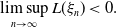 $\limsup \limits _{n\to \infty } L(\xi _{n})\lt 0.$
Thus, Lemma2.2 shows that there exists a
$\limsup \limits _{n\to \infty } L(\xi _{n})\lt 0.$
Thus, Lemma2.2 shows that there exists a $t_n\in (0,1)$
such that
$t_n\in (0,1)$
such that $(\xi _{n})_{t_{n}}\in \mathcal{M}.$
In addition, it is easy to see that $\limsup \limits _{n\to \infty } t_n\lt 1$
; in fact, arguments by contradiction, along a subsequence
$\limsup \limits _{n\to \infty } t_n\lt 1$
; in fact, arguments by contradiction, along a subsequence $t_{n}\to 1$
, make that
$t_{n}\to 1$
, make that $L(\xi _{n})=L(\xi _{n})_{t_{n}}+o_{n}(1)=o_{n}(1);$
this is also impossible. Since
$L(\xi _{n})=L(\xi _{n})_{t_{n}}+o_{n}(1)=o_{n}(1);$
this is also impossible. Since $w_n\in \mathcal{M},$
in view of (2.13) and (2.17), it is found that
$w_n\in \mathcal{M},$
in view of (2.13) and (2.17), it is found that
 \begin{align*} m+o_{n}(1)& =I(w_{n})-\frac {1}{N+p+1}L(w_{n})\\ & =\frac {1}{2(N+p+1)}\Big \{(p+3)\|\Delta w_{n}\|_2^2+\left (p-1\right )\|w_{n}\|_2^2+\frac {\left (p-1\right )}{2}\|\nabla |w_{n}|^2\|_2^2\Big \}\\ & \geq \frac {p+3}{2(N+p+1)}\big \{\|\Delta w\|_2^2+\|\Delta \xi _{n}\|_2^2\big \}+\frac {p-1}{2(N+p+1)}\big \{\|w\|_2^2+\|\xi _{n}\|_2^2\big \}\\ &\,\,\,\,+\frac {p-1}{4\left (N+p+1\right )}\big \{{\|\nabla |w|^2\|_2^2+\|\nabla |\xi _{n}|^2\|_2^2}\big \}\,\,\,\,\\ & =I(w)-\frac {1}{N+p+1}L(w)+I(\xi _{n})-\frac {1}{N+p+1}L(\xi _{n})\\ & \gt I(w)-\frac {1}{N+p+1}L(w)+I(\xi _{n})_{t_{n}}-\frac {1}{N+p+1}L(\xi _{n})_{t_{n}}\\ & =I(\xi _{n})_{t_{n}}+\frac {p+3}{2(N+p+1)}\|\Delta w\|_2^2+\frac {p-1}{2(N+p+1)}\|w\|_2^2\\ & \,\,\,\,+\frac {p-1}{4\left (N+p+1\right )}\|\nabla |w|^2\|_2^2\geq m. \end{align*}
This case is also impossible. Hence, we deduce that $w\in \mathcal{M}$
.
$w\in \mathcal{M}$
.
Next, by using Lebesgue dominated convergence theorem, Fatou’s lemma and $w_n\in \mathcal{M}$
, it follows that
$w_n\in \mathcal{M}$
, it follows that
 \begin{equation*}\begin{aligned}m & \leq I(w)-\frac {1}{N+p+1}L(w)\\[2pt] & =\frac {1}{2(N+p+1)}\left\{(p+3)\|\Delta w\|_2^2+\left (p-1\right )\|w\|_2^2+\frac {p-1}{2}\|\nabla |w|^2\|_2^2\right\}\\[2pt] & \leq \frac {1}{2(N+p+1)}\liminf _{n\to \infty }\left\{(p+3){}\|\Delta w_{n}\|_2^2+\left (p-1\right )\|w_{n}\|_2^2+\frac {p-1}{2}\|\nabla |w_{n}|^2\|_2^2\right\}\\[2pt] & =\liminf _{n\to \infty }\bigg[I(w_{n})-\frac {1}{N+p+1}L(w_{n})\bigg]\\[2pt] & =\liminf _{n\to \infty }I(w_{n})=m.\end{aligned}\end{equation*}
Thus, we get that $\|w_n\|_{H}\to \|w\|_{H}$
and
$\|w_n\|_{H}\to \|w\|_{H}$
and $I(w)=m$
, which means that there exists a minimum
$I(w)=m$
, which means that there exists a minimum $m$
of
$m$
of $I|_{\mathcal{M}}$
. In fact, by arguments similar to those in Lemma2.5 of [Reference Liu, Wang and Wang34],
$I|_{\mathcal{M}}$
. In fact, by arguments similar to those in Lemma2.5 of [Reference Liu, Wang and Wang34], $w$
is indeed a solution of (1.9). We thereby complete the proof of this lemma.
$w$
is indeed a solution of (1.9). We thereby complete the proof of this lemma.
2.2. Proof of Theorem1.1
Building upon the lemmas above, we are now in the position to give the proof of the existence of standing wave solutions to Cauchy problem (1.1).
Proof. Suppose that $\tilde {w}\in \mathcal{M}$
is a minimizer of the functional
$\tilde {w}\in \mathcal{M}$
is a minimizer of the functional $I|_{\mathcal{M}}$
. Then, applying Lemma2.2, we see that
$I|_{\mathcal{M}}$
. Then, applying Lemma2.2, we see that
 \begin{equation*}I(\tilde {w})=\inf _{w\in H}\max _{t\gt 0}I(w_{t})=m.\end{equation*}
Proceeding by contradiction, we assume that $\tilde {w}$
is not a weak solution to equation (1.9). Thus, we can find that there exists
$\tilde {w}$
is not a weak solution to equation (1.9). Thus, we can find that there exists $\phi \in C_0^{\infty }(\mathbb{R}^{N})$
such that
$\phi \in C_0^{\infty }(\mathbb{R}^{N})$
such that
 \begin{equation*}\begin{aligned} \langle I^{\prime }(\tilde {w}),\phi \rangle =\int _{\mathbb{R}^{N}}(\Delta \tilde {w}\Delta \phi +\nabla (\tilde {w}^2)\nabla (\tilde {w}\phi )+\tilde {w}\phi -|\tilde {w}|^{p-1}\tilde {w}\phi )dy\lt -1.\end{aligned}\end{equation*}
Owing to the continuous property of $I^{\prime }(\tilde {w}_t)$
, we can choose a sufficiently small
$I^{\prime }(\tilde {w}_t)$
, we can choose a sufficiently small $\varepsilon \gt 0$
such that
$\varepsilon \gt 0$
such that
 \begin{equation*}\left \langle I^{\prime }(\tilde {w}_{t}+\sigma \phi ),\phi \right \rangle \leq -\frac {1}{2},\quad |t-1|\leq \varepsilon ,\,\,|\sigma |\leq \varepsilon .\end{equation*}
Furthermore, we introduce a cut-off function $\zeta (t)$
in form
$\zeta (t)$
in form
 \begin{equation*}\left .\zeta (t)\,:\!=\,\left \{\begin{array}{ll}\zeta (t)=1,&\quad |t-1|\leq \frac \varepsilon 2, \\[2pt] 0\leq \zeta (t)\leq 1,&\quad \frac \varepsilon 2\lt |t-1|\lt \varepsilon , \\[2pt] \zeta (t)=0,&\quad |t-1|\geq \varepsilon , \end{array}\right .\right .\end{equation*}
and then define the function
 \begin{equation*}\gamma (t)\,:\!=\,\left \{\begin{array}{ll}\tilde {w}_t,&\quad \left |t-1\right |\geq \varepsilon ,\\ \tilde {w}_t+\varepsilon \zeta (t)\phi , &\quad \left |t-1\right |\lt \varepsilon .\end{array}\right .\end{equation*}
Thus, note that $\gamma (t)$
is a continuous curve endowed with metric
$\gamma (t)$
is a continuous curve endowed with metric $(H,d_{H})$
. We further choose a smaller
$(H,d_{H})$
. We further choose a smaller $\varepsilon$
such that
$\varepsilon$
such that $d_{H}(\gamma (t),0)\gt 0$
for
$d_{H}(\gamma (t),0)\gt 0$
for $|t-1|\lt \varepsilon$
.
$|t-1|\lt \varepsilon$
.
First, we shall claim that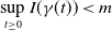 $\sup \limits _{t\geq 0}I(\gamma (t))\lt m$
. In fact, if
$\sup \limits _{t\geq 0}I(\gamma (t))\lt m$
. In fact, if $\left |t-1\right |\geq \varepsilon$
, we have
$\left |t-1\right |\geq \varepsilon$
, we have
 \begin{equation*}I(\gamma (t))=I(\tilde {w}_{t})\lt I(\tilde {w})=m.\end{equation*}
If $\left |t-1\right |\lt \varepsilon$
, we define a
$\left |t-1\right |\lt \varepsilon$
, we define a $\mathrm{C}^1$
map
$\mathrm{C}^1$
map $\sigma \mapsto I(\tilde {w}_{t}+\sigma \zeta (t)\phi )\in \mathbb{R}$
, where
$\sigma \mapsto I(\tilde {w}_{t}+\sigma \zeta (t)\phi )\in \mathbb{R}$
, where $\sigma \in \left [0,\varepsilon \right ]$
. Using the mean value theorem, it is easy to see that for a suitable
$\sigma \in \left [0,\varepsilon \right ]$
. Using the mean value theorem, it is easy to see that for a suitable $\bar {\sigma }\in (0,\sigma ),$
 \begin{equation*}\begin{aligned}I (\tilde {w}_{t}+\sigma \zeta (t)\phi ) &=I(\tilde {w}_{t})+\langle I^{\prime }(\tilde {w}_{t}+\bar {\sigma }\zeta (t)\phi ,\zeta (t)\phi \bar {\sigma }\rangle \\ & \leq I(\tilde {w}_{t})-\frac {1}{2}\lt m.\end{aligned}\end{equation*}
Next, since $I(\tilde {w}_{t})=h_{\tilde {w}}(t)$
and
$I(\tilde {w}_{t})=h_{\tilde {w}}(t)$
and $h_{\tilde {w}}^{^{\prime }}(1)=0=L(\tilde {w})$
, we observe that
$h_{\tilde {w}}^{^{\prime }}(1)=0=L(\tilde {w})$
, we observe that
 \begin{equation*}L(\gamma (1-\varepsilon ))\gt 0,\,\text{for}\,t=1-\varepsilon ,\end{equation*}
and
 \begin{equation*}L(\gamma (1+\varepsilon ))\lt 0,\,\text{for}\,t=1+\varepsilon .\end{equation*}
Applying the continuity of $t\mapsto L(\gamma (t)),$
we obtain that there exists a
$t\mapsto L(\gamma (t)),$
we obtain that there exists a $t_{0}\in (1-\varepsilon ,1+\varepsilon )$
such that
$t_{0}\in (1-\varepsilon ,1+\varepsilon )$
such that $L(\gamma (t_0))=0$
, that is
$L(\gamma (t_0))=0$
, that is
 \begin{equation*} (\gamma (t_0))=(\tilde {w}_{t_0}+\varepsilon \zeta (t_0)\phi )\in \mathcal{M}.\end{equation*}
Thus, by the definition of $m$
, we have that
$m$
, we have that
 \begin{equation*}I(\gamma (t_0))\lt m,\end{equation*}
which is a contradiction. We deduce that $\tilde {w}$
is a weak solution of system (1.9). By similar arguments to those in steps 2 and 3 of Lemma2.8, it follows that
$\tilde {w}$
is a weak solution of system (1.9). By similar arguments to those in steps 2 and 3 of Lemma2.8, it follows that $\tilde {w}\neq 0$
. Since any solution of (1.9) belongs to
$\tilde {w}\neq 0$
. Since any solution of (1.9) belongs to $\mathcal{M}$
, its minimizer is a ground state solution. Thereby, we conclude that the Cauchy problem (1.1) has the standing wave solutions in form (1.8). This completed the proof of Theorem1.1.
$\mathcal{M}$
, its minimizer is a ground state solution. Thereby, we conclude that the Cauchy problem (1.1) has the standing wave solutions in form (1.8). This completed the proof of Theorem1.1.
3. Stability of standing wave solutions
This section investigates the stability (Theorem1.3) of standing wave solution (1.8) to Cauchy problem (1.1) by using concentration-compactness lemmas and variational techniques and methods.
3.1. Auxiliary lemmas and technical preparations
To establish the foundation for our principal conclusions, we begin by introducing some concentration-compactness lemmas and Sobolev-type inequalities related to (1.1).
Lemma 3.1. [Reference Cazenave35, Lemma 1.7.4] Let $u\in L^2$
with
$u\in L^2$
with $\|u\|_{2}^{2}=a\gt 0$
. Further define the concentration function
$\|u\|_{2}^{2}=a\gt 0$
. Further define the concentration function $\rho (u,r)$
in form
$\rho (u,r)$
in form
 \begin{equation} \rho (u,r)=\sup _{y\in \mathbb{R}^N}\int \limits _{\{|x-y|\lt r\}}|u(x)|^2dx,\quad \text{for}\,r\gt 0, \end{equation}
then we have that $(1)$
$(1)$ $\rho (u,r)$
is an increasing function of
$\rho (u,r)$
is an increasing function of $r$
and satisfies
$r$
and satisfies
 \begin{equation*}\begin{cases}\rho (u,0)=0,\ \ \ \ \lim \limits _{r\to \infty }\rho (u,r)=a,\\ 0\lt \rho (u,r)\leq a,\,\, \text{for}\, r\gt 0;&\end{cases} \end{equation*} $(2)$
There exists a
$(2)$
There exists a $y(u,r)\in \mathbb{R}^{N}$
such that
$y(u,r)\in \mathbb{R}^{N}$
such that
 \begin{equation*}\rho (u,r)=\int \limits _{\{|x-y(u,r)|\lt r\}}\big |u(x)\big |^2dx;\end{equation*} $(3)$
There exists a positive constant
$(3)$
There exists a positive constant $C=C(N,q)$
such that for
$C=C(N,q)$
such that for $u\in L^{q}$
with some
$u\in L^{q}$
with some $q\gt 2$
,
$q\gt 2$
,
 \begin{equation*}\left |\rho (u,r)-\rho (u,s)\right |\leq C(N,q)\left |r^{N}-s^{N}\right |^{\frac {q-2}{q}}\|u\|_{{q}}^2,\quad \text{for all}\,r,s\gt 0.\end{equation*}
We will proceed by examining two scenarios: one case is $1\lt p\lt +\infty$
, when
$1\lt p\lt +\infty$
, when $2\lt N\leq 4$
and
$2\lt N\leq 4$
and $1\lt p\lt \frac {N+4}{N-4}$
, when
$1\lt p\lt \frac {N+4}{N-4}$
, when $4\lt N\leq 6$
; another case is
$4\lt N\leq 6$
; another case is $1\lt p\lt \frac {3N+2}{N-2}$
and
$1\lt p\lt \frac {3N+2}{N-2}$
and $N\gt 6$
.
$N\gt 6$
.
For one thing, when $2\lt N\leq 6$
, the stability shall be discussed in
$2\lt N\leq 6$
, the stability shall be discussed in $H^2$
-norm and some corresponding essential lemmas are presented below.
$H^2$
-norm and some corresponding essential lemmas are presented below.
Lemma 3.2.
For any $u\in H^2$
,
$u\in H^2$
, $r\gt 0$
and
$r\gt 0$
and $2\lt N\leq 6$
, one can find a constant
$2\lt N\leq 6$
, one can find a constant $K_1$
satisfying
$K_1$
satisfying
 \begin{equation} \|u\|_{\frac {2N+8}N}^{\frac {2N+8}N}\leq K_1\rho (u,r)^{\frac 4N}\|\Delta u\|_2^2, \end{equation}
where $\rho$
is defined by (
3.1
).
$\rho$
is defined by (
3.1
).
Proof. First, we choose a sequence of open, unit cubes of $\mathbb{R}^{N}$
denoted by
$\mathbb{R}^{N}$
denoted by $(Q_{n})_{n\geq 0}$
, which satisfy
$(Q_{n})_{n\geq 0}$
, which satisfy $Q_{n}\cap Q_l=\emptyset$
(
$Q_{n}\cap Q_l=\emptyset$
( $n\neq l$
) and
$n\neq l$
) and $\overline {\cup _{n\geq 0}(Q_{n})}=\mathbb{R}^{N}$
. By the additivity of integration over domains, we obtain that for
$\overline {\cup _{n\geq 0}(Q_{n})}=\mathbb{R}^{N}$
. By the additivity of integration over domains, we obtain that for $\alpha \in \mathbb{R}$
,
$\alpha \in \mathbb{R}$
,
 \begin{equation*}\int \limits _{\mathbb{R}^{N}}\big |u\big |^{\alpha +2}dx=\sum \limits _{n=0}^{\infty }\int \limits _{Q_{n}}\big |u\big |^{\alpha +2}dx,\end{equation*}
and
 \begin{equation*}\int \limits _{\mathbb{R}^{N}}|\Delta u|^2dx=\sum \limits _{n=0}^{\infty }\int \limits _{Q_{n}}|\Delta u|^2dx.\end{equation*}
We further elaborate the analysis through the following two steps. $\mathbf{Step\,1}$
. There exists constant
$\mathbf{Step\,1}$
. There exists constant $C$
independent of
$C$
independent of $n$
such that for all
$n$
such that for all $u\in H(Q_{n})$
,
$u\in H(Q_{n})$
,
 \begin{equation} \begin{aligned} & \int \limits _{Q_{n}}|u|^{\frac {2N+4}N}dx\leq C\bigg (\int \limits _{Q_{n}}|u|^2dx\bigg )^{\frac 2N}\int \limits _{Q_{n}}|\Delta u|^2dx.\quad \end{aligned} \end{equation}
In fact, for $4\lt N\leq 6$
, using the Gargliardo–Nirenberg theorem, we get that
$4\lt N\leq 6$
, using the Gargliardo–Nirenberg theorem, we get that
 \begin{equation} \begin{aligned}\bigg (\int \limits _{Q_{n}}\big |u\big |^{p+1}dx\bigg )^{\frac {1}{p+1}} & \leq C\bigg (\int \limits _{Q_{n}}\big |\Delta u\big |^2dx\bigg )^{\frac {\theta }{2}}\bigg (\int \limits _{Q_{n}}\big |u^2\big |dx\bigg )^{\frac {1-\theta }{2}}\\ & =C\bigg (\int \limits _{Q_{n}}\big |\Delta u\big |^2dx\bigg )^{{\frac {N(p -1)}{8(p+1)}}}\bigg (\int \limits _{Q_{n}}\big |u^2\big |dx\bigg )^{\frac 12-{\frac {N(p-1)}{8(p+1)}}},\end{aligned} \end{equation}
where $\frac {1}{p+1}=\theta \left (\frac {1}{2}-\frac {2}{N}\right )+\frac {(1-\theta )}2,\,1\lt p\lt \frac {N+4}{N-4}.$
Furthermore, taking
$\frac {1}{p+1}=\theta \left (\frac {1}{2}-\frac {2}{N}\right )+\frac {(1-\theta )}2,\,1\lt p\lt \frac {N+4}{N-4}.$
Furthermore, taking $p=\frac {N+8}N$
in (3.4), we deduce that the inequality (3.3) holds for
$p=\frac {N+8}N$
in (3.4), we deduce that the inequality (3.3) holds for $4\lt N\leq 6$
. Especially, choosing
$4\lt N\leq 6$
. Especially, choosing $p=\frac {11}3$
for case
$p=\frac {11}3$
for case $N=3$
and selecting
$N=3$
and selecting $p=3$
for case
$p=3$
for case $N=4$
, it is easy to see that (3.3) holds. Finally, in the aforementioned calculations, the fact that the constant
$N=4$
, it is easy to see that (3.3) holds. Finally, in the aforementioned calculations, the fact that the constant $C$
is independent of
$C$
is independent of $n$
follows from the translation invariance of
$n$
follows from the translation invariance of $|Q_{n}|$
.
$|Q_{n}|$
. $\mathbf{Step\,2}$
. Summing up
$\mathbf{Step\,2}$
. Summing up $n$
in the above inequality (3.3), it follows that
$n$
in the above inequality (3.3), it follows that
 \begin{equation} \begin{aligned}\int \limits _{\mathbb{R}^{N}}|u|^{\frac {2N+8}N}dx\leq C\bigg (\sup \limits _{n\in \mathbb{N}}\int \limits _{Q_{n}}|u|^2dx\bigg )^{\frac 4N}\bigg (\int \limits _{\mathbb{R}^{N}}|\Delta u|^2dx\bigg ).\end{aligned} \end{equation}
Furthermore, changing $u(x)$
to
$u(x)$
to $u(rx)$
in (3.5) gives that
$u(rx)$
in (3.5) gives that
 \begin{equation*}\begin{aligned} & \int \limits _{\mathbb{R}^{N}}|u\left (y\right )|^{\frac {2N+8}N}d(r^{-1}y)\\ & \leq C\bigg (\sup \limits _{n\in \mathbb{N}}\int \limits _{Q_{n}}|u\left (y\right )|^2d(r^{-1}y)\bigg )^{\frac 4N}\bigg (\int \limits _{\mathbb{R}^{N}}|\Delta u\left (y\right )|^2d(r^{-1}y)\bigg ).\end{aligned}\end{equation*}
By direct calculations, we have that
 \begin{equation*}\begin{aligned} & r^{-N}\int \limits _{\mathbb{R}^{N}}|u(y)|^{\frac {2N+8}{N}}dy\\ & \leq C\bigg (r^{-N}\sup \limits _{n\in \mathbb{N}}\int \limits _{Q_{n}}|u\left (y\right )|^2dy\bigg )^{\frac 4N}\bigg (r^{4-N}\int \limits _{\mathbb{R}^{N}}|\Delta u\left (y\right )|^2dy\bigg )\\ & \leq Cr^{-N}\bigg (\sup \limits _{n\in \mathbb{N}}\int \limits _{Q_{n}}|u\left (y\right )|^2dy\bigg )^{\frac 4N}\bigg (\int \limits _{\mathbb{R}^{N}}|\Delta u\left (y\right )|^2dy\bigg ),\end{aligned}\end{equation*}
which, along with definition (3.1) of $\rho (u,r)$
, yields that (3.2) holds.
$\rho (u,r)$
, yields that (3.2) holds.
Lemma 3.3.
Let $\{u_{n}\}_{n=1}^{\infty }\subset H^2$
and satisfy
$\{u_{n}\}_{n=1}^{\infty }\subset H^2$
and satisfy
 \begin{equation} \|u_{n}\|_2^2=a\gt 0,\,\,\,\quad \sup _{n\geq 0}\|\Delta u_{n}\|_2^2\lt \infty . \end{equation}
Further define
 \begin{equation} \sigma =\lim \limits _{r\to \infty }\liminf _{n\to \infty }\rho (u_{n},r), \end{equation}
where $\rho (u_n,r)$
was introduced by (
3.1
). Then, there exists a sequence
$\rho (u_n,r)$
was introduced by (
3.1
). Then, there exists a sequence $\{u_{n_{l}}\}$
, an increasing function
$\{u_{n_{l}}\}$
, an increasing function $\gamma (r)$
and a sequence
$\gamma (r)$
and a sequence $r_{l}\to \infty$
satisfying
$r_{l}\to \infty$
satisfying $(1)$
$(1)$ $\rho (u_{n_{l}},r)\to \gamma (r)\in [0,a]$
uniformly on bounded sets of
$\rho (u_{n_{l}},r)\to \gamma (r)\in [0,a]$
uniformly on bounded sets of $[0,\infty )\,as\,l\to \infty$
;
$[0,\infty )\,as\,l\to \infty$
; $(2)$
$(2)$ $\sigma =\lim \limits _{r\to \infty }\gamma (r)=\lim \limits _{l\to \infty }\rho (u_{n_{l}},r_{l})=\lim \limits _{l\to \infty }\rho (u_{n_{l}},\frac {r_l}{2}).$
Proof. The demonstrations of this lemma employ reasoning analogous to 1.7.5 of [Reference Cazenave35]. The core modification lies in substituting the original condition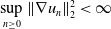 $\sup \limits _{n\geq 0}\|\nabla u_{n}\|_2^2\lt \infty$
with the condition stated above
$\sup \limits _{n\geq 0}\|\nabla u_{n}\|_2^2\lt \infty$
with the condition stated above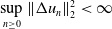 $\sup \limits _{n\geq 0}\|\Delta u_{n}\|_2^2\lt \infty$
. Given the substantial overlap in technical manoeuvres with prior arguments, we elect to omit the details here.
$\sup \limits _{n\geq 0}\|\Delta u_{n}\|_2^2\lt \infty$
. Given the substantial overlap in technical manoeuvres with prior arguments, we elect to omit the details here.
Based on the above Lemmas3.1–3.3, we can establish the lemma related to the approximation of nonlinear terms. Although this lemma shares some similarities with the proof of Proposition 1.7.6 in Ref. [Reference Cazenave35], the main difference and challenge lie in the treatment of the second-order nonlinear derivative term and power-type source in (1.1).
Lemma 3.4.
Under the conditions of Lemma
3.3
, $\rho (u,r)$
and
$\rho (u,r)$
and $\sigma$
were defined in (
3.1
) and (
3.7
), respectively, then there exist the sequence
$\sigma$
were defined in (
3.1
) and (
3.7
), respectively, then there exist the sequence $\{u_{n_{l}}\}$
satisfying,
$\{u_{n_{l}}\}$
satisfying, $(1)$
If
$(1)$
If $\sigma =a$
, then there exist a sequence
$\sigma =a$
, then there exist a sequence $\{y_{l}\}\subset \mathbb{R}^{N}$
and
$\{y_{l}\}\subset \mathbb{R}^{N}$
and $u\in H^2(\mathbb{R}^N)$
such that for
$u\in H^2(\mathbb{R}^N)$
such that for $1\lt p\lt +\infty$
, when
$1\lt p\lt +\infty$
, when $2\lt N\leq 4$
and
$2\lt N\leq 4$
and $1\lt p\lt \frac {N+4}{N-4}$
, when
$1\lt p\lt \frac {N+4}{N-4}$
, when $4\lt N\leq 6$
,
$4\lt N\leq 6$
,
 \begin{equation*}u_{n_{l}}({\cdot} -y_{l})\to u\ \ \text{in}\ \ L^{p+1}(\mathbb{R}^N),\ \ \ \text{as}\ \ l\to +\infty ;\end{equation*} $(2)$
If
$(2)$
If $\sigma =0$
, then there exist a sequence
$\sigma =0$
, then there exist a sequence $\{y_{l}\}\subset \mathbb{R}^{N}$
such that for
$\{y_{l}\}\subset \mathbb{R}^{N}$
such that for $1\lt p\lt +\infty$
, when
$1\lt p\lt +\infty$
, when $2\lt N\leq 4$
and
$2\lt N\leq 4$
and $1\lt p\lt \frac {N+4}{N-4}$
, when
$1\lt p\lt \frac {N+4}{N-4}$
, when $4\lt N\leq 6$
,
$4\lt N\leq 6$
,
 \begin{equation*}u_{n_{l}}({\cdot} -y_{l})\to 0\ \ \ \text{in}\ \ L^{p+1}(\mathbb{R}^N),\ \ \ \text{as}\ \ l\to +\infty ;\end{equation*} $(3)$
There exist
$(3)$
There exist $v_{l}\subset H^2(\mathbb{R}^N)$
and
$v_{l}\subset H^2(\mathbb{R}^N)$
and $w_{l}\subset H^2(\mathbb{R}^N)$
such that for
$w_{l}\subset H^2(\mathbb{R}^N)$
such that for $1\lt p\lt +\infty$
, when
$1\lt p\lt +\infty$
, when $2\lt N\leq 4$
and
$2\lt N\leq 4$
and $1\lt p\lt \frac {N+4}{N-4}$
, when
$1\lt p\lt \frac {N+4}{N-4}$
, when $4\lt N\leq 6$
,
$4\lt N\leq 6$
,
 \begin{equation} \begin{aligned} \operatorname {supp}v_{l}\cap \operatorname {supp}w_{l}=\emptyset ,\quad \end{aligned} \end{equation}
 \begin{equation} \begin{aligned} |v_{l}|+|w_{l}|\leq |u_{n_{l}}|,\quad \|v_{l}\|_{H^2}+\|w_{l}\|_{H^2}\leq C\|u_{n_{l}}\|_{H^2}, \end{aligned} \end{equation}
 \begin{equation} \begin{aligned} \|\nabla |v_{l}|^2\|_2^2+\|\nabla |w_{l}|^2\|_2^2\leq C\|\nabla |u_{n_{l}}|^2\|_2^2, \end{aligned} \end{equation}
 \begin{equation} \begin{aligned} \|v_{l}\|_2^2\to \sigma ,\quad \|w_{l}\|_2^2\to a-\sigma ,\quad l\to \infty , \end{aligned} \end{equation}
 \begin{equation} \begin{aligned} \liminf _{l\to \infty }\left (\|\Delta u_{n_{l}}\|_2^2-\|\Delta v_{l}\|_2^2-\|\Delta w_{l}\|_2^2\right )\geq 0, \end{aligned} \end{equation}
 \begin{equation} \begin{aligned} \liminf _{l\to \infty }\big(\|\nabla |u_{n_{l}}|^2\|_2^2-\|\nabla |v_{l}|^2\|_2^2-\|\nabla |w_{l}|^2\|_2^2\big)\geq 0, \end{aligned} \end{equation}
 \begin{equation} \begin{aligned} \big |\|u_{n_{l}}\|_{p+1}^{p+1}-\|v_{l}\|_{p+1}^{p+1}-\|w_{l}\|_{p+1}^{p+1}\big |\to 0,\quad l\to \infty . \end{aligned} \end{equation}
Proof. Let the functions $\gamma ({\cdot} )$
and
$\gamma ({\cdot} )$
and $y({\cdot} ,\cdot )$
, and the sequences
$y({\cdot} ,\cdot )$
, and the sequences $(u_{n_{l}})_{l\geq 0}$
and
$(u_{n_{l}})_{l\geq 0}$
and $\left (r_{l}\right )_{l\geq 0}$
, be defined as in Lemmas3.1 and 3.3. Choosing
$\left (r_{l}\right )_{l\geq 0}$
, be defined as in Lemmas3.1 and 3.3. Choosing $\widetilde {r}$
sufficiently large so that
$\widetilde {r}$
sufficiently large so that $\gamma (\widetilde {r})\gt \frac a{2}$
and letting
$\gamma (\widetilde {r})\gt \frac a{2}$
and letting $y_{l}=y(u_{n_{l}},\widetilde {r})$
. By standard subsequence arguments, we may assume that there exists
$y_{l}=y(u_{n_{l}},\widetilde {r})$
. By standard subsequence arguments, we may assume that there exists $u\in H^2$
such that
$u\in H^2$
such that
 \begin{equation} u_{n_l}({\cdot} -y_l)\rightharpoonup u\quad \mathrm{in\,}{H^2}(\mathbb{R}^N)\mathrm{\,as\,}l\to \infty . \end{equation}
Now, the proof proceeds in the following three steps: $\mathbf{Step\,1}$
. Establishing that part (1) holds.
$\mathbf{Step\,1}$
. Establishing that part (1) holds.
When $\sigma =a$
, we can assert that if
$\sigma =a$
, we can assert that if $u$
is given by (3.15), then
$u$
is given by (3.15), then
 \begin{equation} \|u\|_{2}^2=a. \end{equation}
Further, by applying (3.16), we can show that (1) holds.
We first prove that the claim (3.16) holds. Since the embedding $H^2(B_{R})\hookrightarrow L^{2}(B_{R})$
is compact, it follows that
$H^2(B_{R})\hookrightarrow L^{2}(B_{R})$
is compact, it follows that
 \begin{equation} \int \limits _{\{|x|\lt R\}}|u(x)|^2dx=\lim \limits _{l\to \infty }\int \limits _{\{|x-y_{l}|\lt R\}}|u_{n_{l}}(x)|^2dx,\quad \text{for every}\,R\gt 0. \end{equation}
On the other hand, by the previous arguments, we have that $\rho (u_{n_{l}},\widetilde {r})\gt \frac a{2}$
for
$\rho (u_{n_{l}},\widetilde {r})\gt \frac a{2}$
for $l$
large enough. Choosing
$l$
large enough. Choosing $\varepsilon \lt \frac a{2}$
and taking
$\varepsilon \lt \frac a{2}$
and taking $\tau$
large so that
$\tau$
large so that $\rho (u_{n_{l}},\tau )\gt a-\varepsilon$
. Thus, we have that for
$\rho (u_{n_{l}},\tau )\gt a-\varepsilon$
. Thus, we have that for $l$
large enough,
$l$
large enough,
 \begin{equation*}\int \limits _{\{|x-y_{l}|\lt \widetilde {r}\}}|u_{n_{l}}|^2dx+\int \limits _{\{|x-y\left (u_{n_{l}}\tau )|\lt \tau \}\right .}|u_{n_{l}}|^2dx\gt \frac {a}{2}+a-\varepsilon \gt a,\end{equation*}
where $\{|x-y_{l}|\lt \widetilde {r}\}\cap \{|x-y(u_{n_{l}},\tau )|\lt \tau \}\neq \varnothing$
. Particularly, when
$\{|x-y_{l}|\lt \widetilde {r}\}\cap \{|x-y(u_{n_{l}},\tau )|\lt \tau \}\neq \varnothing$
. Particularly, when $R=\widetilde {r}+2\tau$
, it follows that
$R=\widetilde {r}+2\tau$
, it follows that $\{|x-y\left (u_{n_{l}},\tau \right )|\lt \tau \}\subset \{|x-y_{l}|\lt R\}$
. So for
$\{|x-y\left (u_{n_{l}},\tau \right )|\lt \tau \}\subset \{|x-y_{l}|\lt R\}$
. So for $l$
large enough, there appears the relation
$l$
large enough, there appears the relation
 \begin{equation*}\int \limits _{\{|x-y_{l}|\lt R\}}|u_{n_{l}}|^2dx\geq \int \limits _{\{|x-y\left (u_{n_{l}},\tau )|\lt \tau \}\right .}|u_{n_{l}}|^2dx\gt a-\varepsilon ,\end{equation*}
which together with (3.17) yields that
 \begin{equation*}\|u\|_2^2\geq \int \limits _{\{|x|\lt R\}}|u\left (x\right )|^2dx\geq a-\varepsilon .\end{equation*}
Letting $\varepsilon \to 0$
, we get that (3.16) holds.
$\varepsilon \to 0$
, we get that (3.16) holds.
Furthermore, $1\lt p\lt +\infty$
, when
$1\lt p\lt +\infty$
, when $2\lt N\leq 4$
and
$2\lt N\leq 4$
and $1\lt p\lt \frac {N+4}{N-4}$
, when
$1\lt p\lt \frac {N+4}{N-4}$
, when $4\lt N\leq 6$
, similar arguments as in (3.4) give that
$4\lt N\leq 6$
, similar arguments as in (3.4) give that
 \begin{equation} \|u_{{n_{l}}}\|_{p+1}\leq C\|\Delta u_{{n_{l}}}\|_2^{\theta }\|u_{{n_{l}}}\|_2^{1-\theta },\,\, \end{equation}
where $\frac {1}{p+1}=\theta \left (\frac {1}{2}-\frac {2}{N}\right )+\frac {(1-\theta )}2$
and
$\frac {1}{p+1}=\theta \left (\frac {1}{2}-\frac {2}{N}\right )+\frac {(1-\theta )}2$
and $0\lt \theta \lt 1$
. In view of (3.6), (3.16), and (3.18), we deduce that
$0\lt \theta \lt 1$
. In view of (3.6), (3.16), and (3.18), we deduce that
 \begin{equation} \begin{aligned}\|u_{{n_{l}}}\|_{p+1}^{p+1}\leq C\|\Delta u_{{n_{l}}}\|_2^{\theta (p+1)}\|u_{{n_{l}}}\|_2^{(1-\theta)(p+1)}\lt +\infty , \end{aligned} \end{equation}
which shows that (1) holds. $\mathbf{Step\,2}$
. Demonstrating that part (2) holds.
$\mathbf{Step\,2}$
. Demonstrating that part (2) holds.
If $\sigma =0$
, it follows from Lemma3.3 that
$\sigma =0$
, it follows from Lemma3.3 that $\rho (u_{n_{l}},r_{l})\to 0$
as
$\rho (u_{n_{l}},r_{l})\to 0$
as $l\to \infty$
, which implies that
$l\to \infty$
, which implies that
 \begin{equation} \|u\|_2^2=\lim \limits _{l\to \infty }\|u_{{n_{l}}}\|_2^2\leq \lim \limits _{l\to \infty }\sup \limits _{y\in \mathbb{R}^{N}}\int \limits _{\{|x-y^{}|\lt r\}}|u_{{n_{l}}}|^2dx=0. \end{equation}
The same arguments as (3.19), we have from (3.6) and (3.20) that
 \begin{equation} \begin{aligned}\|u_{{n_{l}}}\|_{p+1}^{p+1} & \leq C\|\Delta u_{{n_{l}}}\|_2^{\theta (p+1)}\|u_{{n_{l}}}\|_2^{(1-\theta)(p+1)}\\[4pt] & \leq C\|u_{{n_{l}}}\|_2^{(1-\theta)(p+1)}\rightarrow 0,\,\,\text{as}\,l\rightarrow \infty .\end{aligned} \end{equation}
So part (2) holds. $\mathbf{Step\,3}$
. Showing that part (3) holds.
$\mathbf{Step\,3}$
. Showing that part (3) holds.
Let us select $\theta ,\varphi \in C^\infty ([0,\infty ))$
with
$\theta ,\varphi \in C^\infty ([0,\infty ))$
with $0\leq \theta ,\varphi \leq 1$
and
$0\leq \theta ,\varphi \leq 1$
and
 \begin{equation*}\begin{aligned}\theta (r)\equiv 1\quad \mathrm{for\,}0\leq r\leq \frac {1}{2},\quad \theta (r)\equiv 0\quad \mathrm{for\,}r\geq \frac {3}{4},\\[3pt] \varphi (r)\equiv 0\quad \mathrm{for\,}0\leq r\leq \frac {3}{4},\quad \varphi (r)\equiv 1\quad \mathrm{for\,}r\geq 1,\end{aligned}\end{equation*}
and further define
 \begin{equation*}v_{l}=\theta _{l}u_{n_{l}},\quad w_{l}=\varphi _{l}u_{n_{l}},\end{equation*}
where
 \begin{equation*}\theta _{l}(x)=\theta \bigg (\frac {|x-y(u_{n_{l}},\frac {r_{l}}{2})|}{r_{l}}\bigg ),\quad \varphi _{l}(x)=\varphi \bigg (\frac {|x-y(u_{n_{l}},\frac {r_{l}}{2})|}{r_{l}}\bigg ).\end{equation*}
Note that the properties (3.8)–(3.10) are apparent and can be directly deduced. In addition, a series of calculations gives that
 \begin{equation*}\begin{aligned} \rho \Big (u_{n_{l}},\frac {r_{l}}{2}\Big )&=\int \limits _{\left \{|x-y(u_{n_{l}},\frac {r_{l}}{2})|\leq \frac {r_{l}}{2}\right \}\big .}|u_{n_{l}}|^2dx\\[3pt] & \leq \int \limits _{\mathbb{R}^{N}}|\theta _{l}u_{n_{l}}|^2dx=\int \limits _{\mathbb{R}^{N}}|v_{{l}}|^2dx\\[3pt] & \leq \int \limits _{\left \{|x-y(u_{n_{l}},\frac {r_{l}}{2})|\leq r_{l}\right \}\big .}|u_{n_{l}}|^2dx\\[3pt] & \leq \int \limits _{\left \{|x-y(u_{n_{l}},r_{l})|\leq r_{l}\right \}\big .}|u_{n_{l}}|^2dx\leq \rho (u_{n_{l}},r_{l}),\end{aligned}\end{equation*}
which together with Lemma3.1 yields that
 \begin{equation} \|v_{l}\|_{2}^2\longrightarrow \sigma ,\,\,\text{as}\,\,l\rightarrow +\infty . \end{equation}
We denote $z_{l}=u_{n_{l}}-v_{l}-w_{l}$
and then obtain
$z_{l}=u_{n_{l}}-v_{l}-w_{l}$
and then obtain $|z_{l}|\leq |u_{n_{l}}|$
. In addition, it is found that
$|z_{l}|\leq |u_{n_{l}}|$
. In addition, it is found that
 \begin{equation*}\begin{aligned} \int \limits _{\mathbb{R}^{N}}|z_{l}|^2dx & \leq \int \limits _{{\left \{\frac {r_{l}}{2}\leq |x-y(u_{n_{l}},\frac {r_{l}}{2})|\leq r_{l}\right \}}}|u_{n_{l}}|^2dx\\[3pt] & =\int \limits _{\left \{|x-y(u_{n_{l}},\frac {r_{l}}{2})|\leq r_{l}\right \}}|u_{n_{l}}|^2dx-\int \limits _{{\left \{|x-y(u_{n_{l}},\frac {r_{l}}{2})|\leq \frac {r_{l}}{2}\right \}}}|u_{n_{l}}|^2dx\\[3pt] & \leq \int \limits _{\left \{|x-y(u_{n_{l}},r_{l})|\leq r_{l}\right \}}|u_{n_{l}}|^2dx-\int \limits _{\left \{|x-y(u_{n_{l}},\frac {r_{l}}{2})|\leq \frac {r_{l}}{2}\right \}}|u_{n_{l}}|^2dx\\[3pt] & =\rho (u_{n_{l}},r_{l})-\rho \Big (u_{n_{l}},\frac {r_{l}}{2}\Big ),\end{aligned}\end{equation*}
which along with Lemma3.1 yields that
 \begin{equation} \|z_{l}\|_{2}^2\longrightarrow 0,\,\,as\,\,{l\to \infty }. \end{equation}
In view of (3.8), (3.22) and (3.23), we deduce that
 \begin{equation*}\|w_{l}\|_{2}^2\longrightarrow a-\sigma ,\,\,as\,\,{l\to \infty }.\end{equation*}
Thus, we complete the proof of (3.11).
Furthermore, it is easy to see that
 \begin{equation} |\nabla |u_{n_{l}}|^2|^2-|\nabla |v_{l}|^2|^2-|\nabla |w_{l}|^2|^2=|\nabla |u_{n_{l}}|^2|^2-|\nabla |\theta _{l}u_{n_{l}}|^2|^2-|\nabla |\varphi _{l}u_{n_{l}}|^2|^2. \end{equation}
Through a series of calculations, we have
 \begin{equation} \begin{aligned}|\nabla |u_{n_{l}}|^2|^2 & =|\nabla (u_{n_{l}}\overline {u_{n_{l}}})|^2=|u_{n_{l}}\nabla \overline {u_{n_{l}}}+\overline {u_{n_{l}}}\nabla u_{n_{l}}|^2\\[2pt] & =2|u_{n_{l}}|^2|\nabla u_{n_{l}}|^2+(u_{n_{l}})^2(\nabla \overline {u_{n_{l}}})^2+\overline {(u_{n_{l}})^2(\nabla \overline {u_{n_{l}}})^2}\\[2pt] & =2|u_{n_{l}}|^2|\nabla u_{n_{l}}|^2+2\operatorname {Re}\left ((u_{n_{l}})^2(\nabla \overline {u_{n_{l}}})^2\right )\!,\end{aligned} \end{equation}
and
 \begin{equation} \begin{aligned}|\nabla |\theta _{l}u_{n_{l}}|^2|^2 & =|\nabla ((\theta _{l}u_{n_{l}})(\theta _{l}\overline {u_{n_{l}}}))|^2\\[2pt] & =|2\theta _{l}|u_{n_{l}}|^2\nabla \theta _{l}+\theta _{l}^2\overline {u_{n_{l}}}\nabla u_{n_{l}}+\theta _{l}^2u_{n_{l}}\nabla \overline {u_{n_{l}}}|^2\\[2pt] & =4\theta _{l}^2|u_{n_{l}}|^4|\nabla \theta _{l}|^2+2\theta _{l}^4|u_{n_{l}}|^2|\nabla u_{n_{l}}|^2\\[2pt] & \,\,\,+4\theta _{l}^3|u_{n_{l}}|^2\nabla \theta _{l}(u_{n_{l}}\nabla \overline {u_{n_{l}}}+\overline {u_{n_{l}}}\nabla u_{n_{l}})\\[2pt] & \,\,\,+\theta _{l}^4\left (\overline {u_{n_{l}}}^2(\nabla u_{n_{l}})^2+u_{n_{l}}^2(\nabla \overline {u_{n_{l}}})^2\right )\\[2pt] & =4\theta _{l}^2|u_{n_{l}}|^4|\nabla \theta _{l}|^2+2\theta _{l}^4|u_{n_{l}}|^2|\nabla u_{n_{l}}|^2\\[2pt] & \,\,\,+8\theta _{l}^3|u_{n_{l}}|^2\nabla \theta _{l}\operatorname {Re}(u_{n_{l}}\nabla \overline {u_{n_{l}}})+2\theta _{l}^4\operatorname {Re}\left (u_{n_{l}}^2(\nabla \overline {u_{n_{l}}})^2\right )\!.\end{aligned} \end{equation}
Using the similar calculations, we have
 \begin{equation} \begin{aligned}|\nabla |\varphi _{l}u_{n_{l}}|^2|^2 & =4\varphi _{l}^2|u_{n_{l}}|^4|\nabla \varphi _{l}|^2+2\varphi _{l}^4|u_{n_{l}}|^2|\nabla u_{n_{l}}|^2 & \\[2pt] & \,\,\,\,+8\varphi _{l}^3|u_{n_{l}}|^2\nabla \varphi _{l}\operatorname {Re}(u_{n_{l}}\nabla \overline {u_{n_{l}}})+2\varphi _{l}^4\operatorname {Re}\left (u_{n_{l}}^2(\nabla \overline {u_{n_{l}}})^2\right )\!. \end{aligned} \end{equation}
Inserting (3.25)–(3.27) into (3.24), it follows that
 \begin{equation} \begin{aligned} & |\nabla |u_{n_{l}}|^2|^2-|\nabla |v_{l}|^2|^2-|\nabla |w_{l}|^2|^2\\[2pt] & =2\left (1-\theta _{l}^4-\varphi _{l}^4\right )|u_{n_{l}}|^2|\nabla u_{n_{l}}|^2\\[2pt] & \,\,\,-4|u_{n_{l}}|^4\left (\theta _{l}^2|\nabla \theta _{l}|^2+\varphi _{l}^2|\nabla \varphi _{l}|^2\right )\\[2pt] & \,\,\,-8\left (\theta _{l}^3\nabla \theta _{l}+\varphi _{l}^3\nabla \varphi _{l}\right )|u_{n_{l}}|^2\operatorname {Re}(u_{n_{l}}\nabla \overline {u_{n_{l}}})\\[2pt] & \,\,\,+2\left (1-\theta _{l}^4-\varphi _{l}^4\right )\operatorname {Re}\left (u_{n_{l}}^2(\nabla \overline {u_{n_{l}}})^2\right )\\[2pt] & \geq -\frac {C}{r_{l}^4}|u_{n_{l}}|^4-\frac {C}{r_{l}^4}|u_{n_{l}}|^3|\nabla u_{n_{l}}|.\end{aligned} \end{equation}
Taking the limit on both sides of (3.24) as $l\rightarrow +\infty$
, we can get that (3.13) holds. Adapting the same way, we can conclude (3.12).
$l\rightarrow +\infty$
, we can get that (3.13) holds. Adapting the same way, we can conclude (3.12).
Next, we denote $s=\frac {|x-y(u_{n_{l}},\frac {r_{l}}{2})|}{r_{l}}$
and discuss through the following three cases.
$s=\frac {|x-y(u_{n_{l}},\frac {r_{l}}{2})|}{r_{l}}$
and discuss through the following three cases. $\mathbf{Case\,1}$
. If
$\mathbf{Case\,1}$
. If $s\in [0,\frac {1}{2}]$
, we have
$s\in [0,\frac {1}{2}]$
, we have $\theta _{l}(s)=1$
and
$\theta _{l}(s)=1$
and $\varphi _{l}(s)=0$
, which implies that
$\varphi _{l}(s)=0$
, which implies that $v_{l}=u_{n_{l}}$
and
$v_{l}=u_{n_{l}}$
and $w_{l}=0$
. In this situation, (3.14) obviously holds.
$w_{l}=0$
. In this situation, (3.14) obviously holds. $\mathbf{Case\,2}$
. When
$\mathbf{Case\,2}$
. When $s\in [\frac {3}{4},+\infty )$
, we have
$s\in [\frac {3}{4},+\infty )$
, we have $\theta _{l}(x)=0$
and
$\theta _{l}(x)=0$
and $\varphi _{l}(x)=1$
, which implies that
$\varphi _{l}(x)=1$
, which implies that $w_{l}=u_{n_{l}}$
and
$w_{l}=u_{n_{l}}$
and $v_{l}=0$
. (3.14) clearly holds.
$v_{l}=0$
. (3.14) clearly holds. $\mathbf{Case\,3}$
. For
$\mathbf{Case\,3}$
. For $s\in (\frac {1}{2},\frac {3}{4})$
, we first verify that
$s\in (\frac {1}{2},\frac {3}{4})$
, we first verify that
 \begin{equation*}\left ||u_{n_{l}}|^{p+1}-|v_{l}|^{p+1}-|w_{l}|^{p+1}\right |\leq C|u_{n_{l}}|^{p}|z_{l}|.\end{equation*}
In fact, if $s\in (\frac {1}{2},\frac {3}{4})$
, then
$s\in (\frac {1}{2},\frac {3}{4})$
, then $\varphi _{l}(s)=0$
and
$\varphi _{l}(s)=0$
and $0\lt \theta _{l}(s)\lt 1$
. Thus, we have
$0\lt \theta _{l}(s)\lt 1$
. Thus, we have $w_{l}=0$
and
$w_{l}=0$
and
 \begin{equation*}|z_{l}|=|u_{n_{l}}-v_{l}|=|u_{n_{l}}-\theta _{l}u_{n_{l}}|=|u_{n_{l}}(1-\theta _{l})|.\end{equation*}
Furthermore, by a series of calculations, we find that
 \begin{equation} \begin{aligned} & \left ||u_{n_{l}}|^{p+1}-|\theta _{l}u_{n_{l}}|^{p+1}\right |\leq |u_{n_{l}}|^{p+1}\left (1-\theta _{l}^{p+1}\right )\\ & =|u_{n_{l}}|^{p+1}\left (1-\theta _{l}\right )\left (1+\theta _{l}+\theta _{l}^2+\cdots +\theta _{l}^{p}\right )\\ & \leq C|u_{n_{l}}|^{p+1}\left (1-\theta _{l}\right )\leq C|u_{n_{l}}|^{p}(u_{n_{l}}-u_{n_{l}}\theta _{l})\\ & =C|u_{n_{l}}|^{p}|z_{l}|.\end{aligned} \end{equation}
Using Hölder inequality, we can get that
 \begin{equation*}\int _{\mathbb{R}^{N}}|u_{n_{l}}|^{p}|z_{l}|dx\leq \|u_{n_{l}}\|_{p+1}^{p}\|z_{l}\|_{p+1}^{p+1}.\end{equation*}
Let $1\lt p\lt +\infty$
, when
$1\lt p\lt +\infty$
, when $2\lt N\leq 4$
and
$2\lt N\leq 4$
and $1\lt p\lt \frac {N+4}{N-4}$
, when
$1\lt p\lt \frac {N+4}{N-4}$
, when $4\lt N\leq 6$
. In the same way as (3.19) and (3.21), we have
$4\lt N\leq 6$
. In the same way as (3.19) and (3.21), we have
 \begin{equation*}\|z_{l}\|_{p+1}^{p+1}\leq C\|\Delta z_{l}\|_2^{\theta (p+1)}\|z_{l}\|_2^{(1-\theta)(p+1)},\end{equation*}
where $\frac {1}{p+1}=\theta \left (\frac {1}{2}-\frac {2}{N}\right )+\frac {(1-\theta )}2$
and
$\frac {1}{p+1}=\theta \left (\frac {1}{2}-\frac {2}{N}\right )+\frac {(1-\theta )}2$
and $0\lt \theta \lt 1$
. Note that
$0\lt \theta \lt 1$
. Note that $z_l$
is bounded in
$z_l$
is bounded in $H^2$
and converges to
$H^2$
and converges to $0$
in
$0$
in $L^2$
. Hence, (3.14) holds. We thereby complete the proof of this lemma.
$L^2$
. Hence, (3.14) holds. We thereby complete the proof of this lemma.
For another thing, when $N\gt 6$
, the stability will be analysed in
$N\gt 6$
, the stability will be analysed in $\bar {H}$
-norm, and some essential lemmas are given below.
$\bar {H}$
-norm, and some essential lemmas are given below.
Lemma 3.5.
For any $u\in \bar {H}$
,
$u\in \bar {H}$
, $r\gt 0$
and
$r\gt 0$
and $N\gt 6$
, one can find a constant
$N\gt 6$
, one can find a constant $K_2$
satisfying
$K_2$
satisfying
 \begin{equation} \|u\|_{\frac {4N+4}N}^{\frac {4N+4}N}\leq K_2\rho (u,r)^{\frac 2N}\|\nabla |u|^2\|_2^2, \end{equation}
where $\rho$
is defined by (
3.1
).
$\rho$
is defined by (
3.1
).
Proof. The proof of this lemma follows the same lines as Lemma3.2. When $N\gt 6$
, by applying Gargliardo–Nirenberg theorem, we have
$N\gt 6$
, by applying Gargliardo–Nirenberg theorem, we have
 \begin{equation} \begin{aligned}\bigg (\int \limits _{Q_{n}}\big |u\big |^{p+1}dx\bigg )^{\frac {2}{p+1}} & \leq C\bigg (\int \limits _{Q_{n}}\big |\nabla |u|^2\big |^2dx\bigg )^{\frac {\theta }{2}}\bigg (\int \limits _{Q_{n}}\big |u^2\big |dx\bigg )^{1-\theta }\\ & =C\bigg (\int \limits _{Q_{n}}\big |\nabla |u|^2\big |^2dx\bigg )^{{\frac {N(p-1)}{\left (N+2\right )(p+1)}}}\bigg (\int \limits _{Q_{n}}\big |u^2\big |dx\bigg )^{1-{\frac {2N(p-1)}{\left (N+2\right )(p+1)}}},\end{aligned} \end{equation}
where $\frac {2}{p+1}=\theta \left (\frac {1}{2}-\frac {1}{N}\right )+(1-\theta),\,1\lt p\lt \frac {3N+2}{N-2}.$
Especially, taking
$\frac {2}{p+1}=\theta \left (\frac {1}{2}-\frac {1}{N}\right )+(1-\theta),\,1\lt p\lt \frac {3N+2}{N-2}.$
Especially, taking $p=\frac {3N+4}N$
in (3.31), then we deduce that there exists constant
$p=\frac {3N+4}N$
in (3.31), then we deduce that there exists constant $C$
independent of
$C$
independent of $n$
such that for all
$n$
such that for all $u\in \bar {H}(Q_{n})$
,
$u\in \bar {H}(Q_{n})$
,
 \begin{equation} \begin{aligned} & \int \limits _{Q_{n}}|u|^{\frac {4N+4}N}dx\leq C\bigg (\int \limits _{Q_{n}}|u|^2dx\bigg )^{\frac 2N}\int \limits _{Q_{n}}|\nabla |u|^2|^2dx.\quad \end{aligned} \end{equation}
Summing on $n$
in (3.32), we get that
$n$
in (3.32), we get that
 \begin{equation} \begin{aligned}\int \limits _{\mathbb{R}^{N}}|u|^{\frac {4N+4}N}dx\leq C\bigg (\sup \limits _{n\in \mathbb{N}}\int \limits _{Q_{n}}|u|^2dx\bigg )^{\frac 2N}\bigg (\int \limits _{\mathbb{R}^{N}}|\nabla |u|^2|^2dx\bigg ).\end{aligned} \end{equation}
Subsequently, changing $u(x)$
to
$u(x)$
to $u(rx)$
in (3.33) and a direct calculations gives that
$u(rx)$
in (3.33) and a direct calculations gives that
 \begin{equation*}\begin{aligned} & r^{-N}\int \limits _{\mathbb{R}^{N}}|u(y)|^{\frac {4N+4}{N}}dy\\ & \leq C\bigg (r^{-N}\sup \limits _{n\in \mathbb{N}}\int \limits _{Q_{n}}|u\left (y\right )|^2dy\bigg )^{\frac 2N}\bigg (r^{2-N}\int \limits _{\mathbb{R}^{N}}|u\left (y\right )\nabla u\left (y\right )|^2dy\bigg )\\ & \leq Cr^{-N}\bigg (\sup \limits _{n\in \mathbb{N}}\int \limits _{Q_{n}}|u\left (y\right )|^2dy\bigg )^{\frac 2N}\bigg (\int \limits _{\mathbb{R}^{N}}|\nabla |u\left (y\right )|^2|^2dy\bigg ).\end{aligned}\end{equation*}
Finally, by applying the definition (3.1) of $\rho (u,r)$
, we conclude that (3.30) holds.
$\rho (u,r)$
, we conclude that (3.30) holds.
Relying on the above Sobolev-type inequality (3.30), we will establish the following two lemmas for $1\lt p\lt \frac {3N+2}{N-2}$
and
$1\lt p\lt \frac {3N+2}{N-2}$
and $N\gt 6$
. It is worth mentioning that the proofs of these lemmas are similar to Lemmas3.3 and 3.4. The main modification in the proof’s processes lies in replacing the norms
$N\gt 6$
. It is worth mentioning that the proofs of these lemmas are similar to Lemmas3.3 and 3.4. The main modification in the proof’s processes lies in replacing the norms $\|\Delta u_{n}\|_2^2$
and
$\|\Delta u_{n}\|_2^2$
and $\|\Delta u\|_2^2$
with
$\|\Delta u\|_2^2$
with $\|\nabla |u_n|^2\|_2^2$
and
$\|\nabla |u_n|^2\|_2^2$
and $\|\nabla |u|^2\|_2^2$
, respectively. Due to the highly repetitive nature of the arguments, we omit the proof’s details.
$\|\nabla |u|^2\|_2^2$
, respectively. Due to the highly repetitive nature of the arguments, we omit the proof’s details.
Lemma 3.6.
Let $\{u_{n}\}_{n=1}^{\infty }\subset \bar {H}$
and satisfy
$\{u_{n}\}_{n=1}^{\infty }\subset \bar {H}$
and satisfy
 \begin{equation} \|u_{n}\|_2^2=a\gt 0,\,\,\,\quad \sup _{n\geq 0}\|u_{n}\|_{\bar {H}}^2\lt \infty . \end{equation}
Further define
 \begin{equation} \sigma =\lim \limits _{r\to \infty }\liminf _{n\to \infty }\rho (u_{n},r), \end{equation}
where $\rho (u_n,r)$
was introduced by (
3.1
). Then, there exist a sequence
$\rho (u_n,r)$
was introduced by (
3.1
). Then, there exist a sequence $\{u_{n_{l}}\}$
, an increasing function
$\{u_{n_{l}}\}$
, an increasing function $\gamma (r)$
and a sequence
$\gamma (r)$
and a sequence $r_{l}\to \infty$
satisfying
$r_{l}\to \infty$
satisfying $(1)$
$(1)$ $\rho (u_{n_{l}},r)\to \gamma (r)\in [0,a]$
uniformly on bounded sets of
$\rho (u_{n_{l}},r)\to \gamma (r)\in [0,a]$
uniformly on bounded sets of $[0,\infty )\,as\,l\to \infty$
;
$[0,\infty )\,as\,l\to \infty$
; $(2)$
$(2)$ $\sigma =\lim \limits _{r\to \infty }\gamma (r)=\lim \limits _{l\to \infty }\rho (u_{n_{l}},r_{l})=\lim \limits _{l\to \infty }\rho (u_{n_{l}},\frac {r_l}{2}).$
Lemma 3.7.
Under the conditions of Lemma
3.6
, $\rho (u,r)$
and
$\rho (u,r)$
and $\sigma$
were defined in (
3.1
) and (
3.35
), respectively, then there exist the sequence
$\sigma$
were defined in (
3.1
) and (
3.35
), respectively, then there exist the sequence $\{u_{n_{l}}\}$
and
$\{u_{n_{l}}\}$
and $1\lt p\lt \frac {3N+2}{N-2}$
when
$1\lt p\lt \frac {3N+2}{N-2}$
when $N\gt 6$
satisfying,
$N\gt 6$
satisfying, $(1)$
If
$(1)$
If $\sigma =a$
, then there exist a sequence
$\sigma =a$
, then there exist a sequence $\{y_{l}\}\subset \mathbb{R}^{N}$
and
$\{y_{l}\}\subset \mathbb{R}^{N}$
and $u\in \bar {H}(\mathbb{R}^N)$
such that
$u\in \bar {H}(\mathbb{R}^N)$
such that
 \begin{equation*}u_{n_{l}}({\cdot} -y_{l})\to u\ \ \text{in}\ \ L^{p+1}(\mathbb{R}^N),\ \ \ \text{as}\ \ l\to +\infty ;\end{equation*} $(2)$
If
$(2)$
If $\sigma =0$
, then there exist a sequence
$\sigma =0$
, then there exist a sequence $\{y_{l}\}\subset \mathbb{R}^{N}$
such that
$\{y_{l}\}\subset \mathbb{R}^{N}$
such that
 \begin{equation*}u_{n_{l}}({\cdot} -y_{l})\to 0\ \ \ \text{in}\ \ L^{p+1}(\mathbb{R}^N),\ \ \ \text{as}\ \ l\to +\infty ;\end{equation*} $(3)$
There exist
$(3)$
There exist $v_{l}\subset \bar {H}(\mathbb{R}^N)$
and
$v_{l}\subset \bar {H}(\mathbb{R}^N)$
and $w_{l}\subset \bar {H}(\mathbb{R}^N)$
such that
$w_{l}\subset \bar {H}(\mathbb{R}^N)$
such that
 \begin{equation} \begin{aligned} \operatorname {supp}v_{l}\cap \operatorname {supp}w_{l}=\emptyset , \end{aligned} \end{equation}
 \begin{equation} \begin{aligned} |v_{l}|+|w_{l}|\leq |u_{n_{l}}|,\quad \|v_{l}\|_{\bar {H}}+\|w_{l}\|_{\bar {H}}\leq C\|u_{n_{l}}\|_{\bar {H}}, \end{aligned} \end{equation}
 \begin{equation} \begin{aligned} \|\nabla |v_{l}|^2\|_2^2+\|\nabla |w_{l}|^2\|_2^2\leq C\|\nabla |u_{n_{l}}|^2\|_2^2, \end{aligned} \end{equation}
 \begin{equation} \begin{aligned} \|v_{l}\|_2^2\to \sigma ,\quad \|w_{l}\|_2^2\to a-\sigma ,\quad l\to \infty , \end{aligned} \end{equation}
 \begin{equation} \begin{aligned} \liminf _{l\to \infty }\left (\|\Delta u_{n_{l}}\|_2^2-\|\Delta v_{l}\|_2^2-\|\Delta w_{l}\|_2^2\right )\geq 0, \end{aligned} \end{equation}
 \begin{equation} \begin{aligned} \liminf _{l\to \infty }\big(\|\nabla |u_{n_{l}}|^2\|_2^2-\|\nabla |v_{l}|^2\|_2^2-\|\nabla |w_{l}|^2\|_2^2\big)\geq 0, \end{aligned} \end{equation}
 \begin{equation} \begin{aligned} \big |\|u_{n_{l}}\|_{p+1}^{p+1}-\|v_{l}\|_{p+1}^{p+1}-\|w_{l}\|_{p+1}^{p+1}\big |\to 0,\quad l\to \infty . \end{aligned} \end{equation}
3.2. Proof of Theorem1.3
In this subsection, we will prove the stability of standing wave solutions (1.8) to Cauchy problem (1.1) through the following analysis.
Proof. $\mathbf{Step\,1}$
. Proving that
$\mathbf{Step\,1}$
. Proving that $0\lt \nu \lt \infty$
. For
$0\lt \nu \lt \infty$
. For $u\in \Gamma$
and
$u\in \Gamma$
and $\lambda \gt 0$
, we define the functional in form
$\lambda \gt 0$
, we define the functional in form
 \begin{equation*}u_{\lambda }(x)=\lambda ^{d}u(\lambda x).\end{equation*}
By a direct calculations, one can verify that $u_{\lambda }\in \Gamma$
and
$u_{\lambda }\in \Gamma$
and
 \begin{equation*}E(u_{\lambda })=\frac {\lambda ^{2d+4-N}}{2}\|\Delta u\|_2^2+\frac {\lambda ^{2(2d+1)-N}}{4}\|\nabla |u|^2\|_2^2-\frac {\lambda ^{d(p+1)-N}}{p+1}\|u\|_{p+1}^{p+1}.\end{equation*}
Choosing $0\lt d\lt \min \{\frac 4{p-1},\frac 2{p-3}\}$
such that
$0\lt d\lt \min \{\frac 4{p-1},\frac 2{p-3}\}$
such that $d(p+1)-N\lt \min \{2d+4-N,4d+2-N\}$
. So it is easy to see that
$d(p+1)-N\lt \min \{2d+4-N,4d+2-N\}$
. So it is easy to see that $E(u_{\lambda })\lt 0$
for
$E(u_{\lambda })\lt 0$
for $\lambda$
small enough. By the definition (1.13), it follows that
$\lambda$
small enough. By the definition (1.13), it follows that $\nu \gt 0$
.
$\nu \gt 0$
.
From Lemma 3 in [Reference Li and Di31], we know that
 \begin{equation*}\begin{aligned}\|u\|_{p+1}^{p+1} & =C\left (p,N\right )\|\nabla |u|^2\|_2^{\frac {pN}{N+2}}\|u\|_2^{^{p+1-\frac {2pN}{N+2}}}\\ & \leq C\left (p,N\right )\left (\|\nabla |u|^2\|_2^2\right )^{\frac {pN}{2(N+2)}}\left (\|u\|_2^2\right )^{\frac {p+1}{2}-\frac {pN}{N+2}}\!.\end{aligned}\end{equation*}
Applying condition $1\lt p\lt \frac {N+2}{N-2}$
, it it found that
$1\lt p\lt \frac {N+2}{N-2}$
, it it found that $\frac {pN}{2(N+2)}\lt 1$
. Taking
$\frac {pN}{2(N+2)}\lt 1$
. Taking $\|u\|_2^2=\|u_0\|_2^2=\tau$
and using Young inequality with
$\|u\|_2^2=\|u_0\|_2^2=\tau$
and using Young inequality with $\epsilon$
, we get that
$\epsilon$
, we get that
 \begin{equation} E(u)\geq \frac {1}{2}\|\Delta u\|_2^2+\left (\frac 14-\epsilon \right )\|\nabla |u|^2\|_2^2-\frac {1}{p+1}C(\varepsilon ,p,N,\tau )\geq -c_2. \end{equation}
We thereby conclude that $-\nu \geq -c_2\gt -\infty .$ $\mathbf{Step\,2}$
. Showing that the minimizing sequence
$\mathbf{Step\,2}$
. Showing that the minimizing sequence $u_n$
of (1.14) is bounded in
$u_n$
of (1.14) is bounded in $H$
and
$H$
and $\|u_{n}\|_{p+1}^{p+1}$
is bounded from below.
$\|u_{n}\|_{p+1}^{p+1}$
is bounded from below.
In fact, by (3.43), one has that $\|\nabla |u_{n}|^2\|_2^2+\|\Delta u_n\|_2^2=\|u_n\|_{\bar H}^2\lt +\infty$
for space dimension
$\|\nabla |u_{n}|^2\|_2^2+\|\Delta u_n\|_2^2=\|u_n\|_{\bar H}^2\lt +\infty$
for space dimension $2\lt N\leq 6$
, and
$2\lt N\leq 6$
, and $\|u_n\|_{H^2}^2\lt +\infty$
for space dimension
$\|u_n\|_{H^2}^2\lt +\infty$
for space dimension $N\gt 6$
is bounded. Furthermore,
$N\gt 6$
is bounded. Furthermore, $u_n\in \Gamma$
implies that
$u_n\in \Gamma$
implies that $u_n$
of (1.12) is bounded in
$u_n$
of (1.12) is bounded in $L^2$
. Since
$L^2$
. Since $\nu \gt 0$
, it is easy to see that
$\nu \gt 0$
, it is easy to see that $E(u_n)\leq -\frac {\nu }{2}$
for
$E(u_n)\leq -\frac {\nu }{2}$
for $n$
large enough. And a series of calculation yields that
$n$
large enough. And a series of calculation yields that
 \begin{equation} \|u_{n}\|_{p+1}^{p+1}=-(p+1)E(u)+\frac {p+1}{2}\|\Delta u\|_2^2+\frac {p+1}{4}\|\nabla |u|^2\|_2^2\geq \frac {p+1}{2}\nu . \end{equation} $\mathbf{Step\,3}$
. Establishing that part (1) holds.
$\mathbf{Step\,3}$
. Establishing that part (1) holds.
In fact, suppose that $\tilde {u}_{n}$
satisfy
$\tilde {u}_{n}$
satisfy $\|\tilde {u}_{n}\|_{2}^{2}\to \sigma$
and
$\|\tilde {u}_{n}\|_{2}^{2}\to \sigma$
and $E(\tilde {u}_{n})\to -\nu ,$
where
$E(\tilde {u}_{n})\to -\nu ,$
where $\sigma$
was introduced in Lemmas3.3 and 3.6. Furthermore, we introduce
$\sigma$
was introduced in Lemmas3.3 and 3.6. Furthermore, we introduce
 \begin{equation*}u_{n}=\sqrt {\frac {\tau }{\|\tilde {u}_{n}\|_2^2}}\tilde {u}_{n},\end{equation*}
and then show that $u_n$
is a minimizing sequence of (1.14). By rescaling, without loss of generality, we may assume that
$u_n$
is a minimizing sequence of (1.14). By rescaling, without loss of generality, we may assume that $\tau =1.$
In addition, we shall apply Lemmas3.3 and 3.6 to
$\tau =1.$
In addition, we shall apply Lemmas3.3 and 3.6 to $u_n$
(minimizing sequence) with
$u_n$
(minimizing sequence) with $a=1$
and prove that
$a=1$
and prove that
 \begin{equation} \sigma =1. \end{equation}
From the proof of above Step 2, we know that $\|u_{n}\|_{p+1}^{p+1}$
is bounded from below, which implies that
$\|u_{n}\|_{p+1}^{p+1}$
is bounded from below, which implies that $\sigma \gt 0$
by Lemmas3.3 and 3.6. Arguing by contradiction, we suppose that
$\sigma \gt 0$
by Lemmas3.3 and 3.6. Arguing by contradiction, we suppose that
 \begin{equation} 0\lt \sigma \lt 1. \end{equation}
In view of (3.12)–(3.14) in Lemma3.4 and (3.40)–(3.42) in Lemma3.7 by the definition of $E(u)$
, one has
$E(u)$
, one has
 \begin{equation*}\liminf _{l\to \infty }(E(u_{n_{l}})-E(v_{l})-E(w_{l}))\geq 0,\end{equation*}
which implies that
 \begin{equation*}\limsup _{l\to \infty }(E(v_{l})+E(w_{l}))\leq \limsup _{l\to \infty }E(u_{n_{l}})\leq -\nu . \end{equation*}
So we have
 \begin{equation} \begin{aligned} \limsup _{l\to \infty }(E(v_{l})+E(w_{l}))\leq -\nu . \end{aligned} \end{equation}
On the other hand, for any $\lambda \gt 0$
and
$\lambda \gt 0$
and $u\in H$
, we discover that
$u\in H$
, we discover that
 \begin{equation*}E(\lambda u)=\frac {1}{2}\|\Delta \lambda u\|_2^2+\frac 14\|\nabla |\lambda u|^2\|_2^2-\frac {1}{p+1}\|\lambda u\|_{p+1}^{p+1},\end{equation*}
which, together with the presentation of $E(u)$
, gives that
$E(u)$
, gives that
 \begin{equation*}\begin{aligned}\frac {1}{\lambda ^2}E(\lambda u) & =\frac {1}{2}\|\Delta u\|_2^2+\frac {\lambda ^2}{4}\|\nabla |u|^2\|_2^2-\frac {\lambda ^{p-1}}{p+1}\|u\|_{p+1}^{p+1}\\[3pt] & =E(u)+\frac {\lambda ^2-1}{4}\|\nabla |u|^2\|_2^2-\frac {\lambda ^{p-1}-1}{p+1}\|u\|_{p+1}^{p+1}.\end{aligned}\end{equation*}
Thus, we get that
 \begin{equation} E(u)=\frac {1}{\lambda ^2}E(\lambda u)+\frac {1-\lambda ^2}{4}\|\nabla |u|^2\|_2^2+\frac {\lambda ^{p-1}-1}{p+1}\|u\|_{p+1}^{p+1}. \end{equation}
Combining (3.47) and (3.48), we have
 \begin{equation*}\begin{gathered}E(v_{l})\geq -\frac {\nu }{a_{l}^{2}}+\frac {1-a_{l}^2}{4}\|\nabla |v_{l}|^2\|_2^2+\frac {a_{l}^{p-1}-1}{p+1}\|v_{l}\|_{p+1}^{p+1}\quad \mathrm{for}\,a_{l}=\frac {1}{\|v_{l}\|_2},\\ E(w_{l})\geq -\frac {\nu }{b_{l}^{2}}+\frac {1-b_{l}^2}{4}\|\nabla |w_{l}|^2\|_2^2+\frac {b_{l}^{p-1}-1}{p+1}\|w_{l}\|_{p+1}^{p+1}\quad \mathrm{for}\,b_{l}=\frac {1}{\|w_{l}\|_2},\end{gathered}\end{equation*}
where $a_{l}(v_{l})\in \Gamma$
and
$a_{l}(v_{l})\in \Gamma$
and $b_{l}(w_{l})\in \Gamma$
. By the definition of
$b_{l}(w_{l})\in \Gamma$
. By the definition of $\|u\|_{p+1}^{p+1}$
, we have
$\|u\|_{p+1}^{p+1}$
, we have
 \begin{equation*}\begin{aligned} & E(v_{l})+E(w_{l}) & \\ & =a_{l}^{-2}E(v_{l})+b_{l}^{-2}E(w_{l})+\frac {1-a_{l}^2}{4}\|\nabla |v_{l}|^2\|_2^2+\frac {1-b_{l}^2}{4}\|\nabla |w_{l}|^2\|_2^2 & \\[2pt] & \,\,\,\,+\left (a_{l^{}}^{p-1}-1\right )\bigg [-E(v_{l})+\frac 12\|\Delta v_{l}\|_2^2+\frac 14\|\nabla |v_{l}|^2\|_2^2\bigg ] & \\[2pt] & \,\,\,\,+\left (b_{l^{}}^{p-1}-1\right )\bigg [-E(w_{l})+\frac 12\|\Delta w_{l}\|_2^2+\frac 14\|\nabla |w_{l}|^2\|_2^2\bigg ] & \\[2pt] & =a_{l}^{-2}E(v_{l})+b_{l}^{-2}E(w_{l})-\left (a_{l}^{p-1}-1\right )E(v_{l})-\left (b_{l}^{p-1}-1\right )E(w_{l}) & \\[2pt] & \,\,\,\,+\frac {a_{l}^{p-1}-a_{l}^2}{4}\|\nabla |v_{l}|^2\|_2^2+\frac {b_{l}^{p-1}-b_{l}^2}{4}\|\nabla |w_{l}|^2\|_2^2 & \\[2pt] & \,\,\,\,+\frac {a_{l}^{p-1}-1}{2}\|\Delta v_{l}\|_2^2+\frac {b_{l}^{p-1}-1}{2}\|\Delta w_{l}\|_2^2. & \end{aligned}\end{equation*}
Since $\|v_l\|_2^2\rightarrow \sigma$
and
$\|v_l\|_2^2\rightarrow \sigma$
and $\|w_l\|_2^2\rightarrow 1-\sigma$
, we have that
$\|w_l\|_2^2\rightarrow 1-\sigma$
, we have that $a_{l}\gt 1, b_{l}\gt 1$
for
$a_{l}\gt 1, b_{l}\gt 1$
for $l$
large enough. According to the conditions
$l$
large enough. According to the conditions $3\lt p\lt +\infty$
when
$3\lt p\lt +\infty$
when $2\lt N\leq 4$
;
$2\lt N\leq 4$
; $3\lt p\lt 3+\frac {16-2N}{N-4}$
when
$3\lt p\lt 3+\frac {16-2N}{N-4}$
when $4\lt N\leq 6$
;
$4\lt N\leq 6$
; $3\lt p\lt 3+\frac {8}{N-2}$
when
$3\lt p\lt 3+\frac {8}{N-2}$
when $N\gt 6$
, we also obtain the following relations:
$N\gt 6$
, we also obtain the following relations:
 \begin{equation*} -\left (a_{l}^{p-1}-1\right )E(v_{l})-\left (b_{l}^{p-1}-1\right )E(w_{l})\gt 0, \end{equation*}
 \begin{equation*} \frac {a_{l}^{p-1}-a_{l}^2}{4}\|\nabla |v_{l}|^2\|_2^2+\frac {b_{l}^{p-1}-b_{l}^2}{4}\|\nabla |w_{l}|^2\|_2^2\gt 0 ,\end{equation*}
 \begin{equation*} \frac {a_{l}^{p-1}-1}{2}\|\Delta v_{l}\|_2^2+\frac {b_{l}^{p-1}-1}{2}\|\Delta w_{l}\|_2^2\gt 0, \end{equation*}
Applying $\|v_l\|_2^2\rightarrow \sigma$
and
$\|v_l\|_2^2\rightarrow \sigma$
and $\|w_l\|_2^2\rightarrow 1-\sigma$
again, we know that
$\|w_l\|_2^2\rightarrow 1-\sigma$
again, we know that $a_{l}^{-2}\to \sigma$
and
$a_{l}^{-2}\to \sigma$
and $ b_{l}^{-2}\to 1-\sigma$
. So we can obtain that
$ b_{l}^{-2}\to 1-\sigma$
. So we can obtain that
 \begin{equation*}\operatorname *{lim}_{l\to \infty }\inf (E(v_{l})+E(w_{l}))\geq a_{l}^{-2}E(v_{l})+b_{l}^{-2}E(w_{l})\gt -\nu ,\end{equation*}
which contradicts (3.47). Hence, $\sigma =1$
.
$\sigma =1$
.
Since $\sigma =a=1$
, by using Lemmas3.4 and 3.7 again, we have that there exists a sequence
$\sigma =a=1$
, by using Lemmas3.4 and 3.7 again, we have that there exists a sequence $\{y_{l}\}\subset \mathbb{R}^{N}$
and some
$\{y_{l}\}\subset \mathbb{R}^{N}$
and some $u\in H$
such that
$u\in H$
such that $u_{n_{l}}({\cdot} -y_{l})\to u$
in
$u_{n_{l}}({\cdot} -y_{l})\to u$
in $L^2$
with
$L^2$
with $u\in \Gamma$
. The weak lower semi-continuity of the
$u\in \Gamma$
. The weak lower semi-continuity of the $H$
norm means that
$H$
norm means that
 \begin{equation*}E(u)\leq \lim _{l\to \infty }E(u_{n_{l}})=-\nu ,\end{equation*}
which, along with the definition of $\nu$
, yields that
$\nu$
, yields that $E(u)=-\nu$
. Thus, we get that
$E(u)=-\nu$
. Thus, we get that $E(u_{n_l})\to E(u)$
. Moreover, using (3.14) and (3.42), we have for
$E(u_{n_l})\to E(u)$
. Moreover, using (3.14) and (3.42), we have for $l\to \infty$
,
$l\to \infty$
,
 \begin{equation*}\|\Delta u_{n_{l}}\|_2^2\to \|\Delta u\|_2^2,\ \ \|\nabla |u_{n_{l}}|^2\|_2^2\to \|\nabla |u|^2\|_2^2,\end{equation*}
which implies that $u_{n_{l}}({\cdot} -y_1)\to u$
strongly in
$u_{n_{l}}({\cdot} -y_1)\to u$
strongly in $H.$
Since
$H.$
Since $\|w\|_2^2=\|u_0\|_2^2$
, we know that the minimizer of (1.14) can be attained at some
$\|w\|_2^2=\|u_0\|_2^2$
, we know that the minimizer of (1.14) can be attained at some $w\in H.$
Similar to corollary 8.3.8 of [Reference Cazenave35], one can verify that
$w\in H.$
Similar to corollary 8.3.8 of [Reference Cazenave35], one can verify that $w\in H$
is also a ground-state solution of the equation
$w\in H$
is also a ground-state solution of the equation
 \begin{equation} \Delta ^2w+w-w\Delta |w|^2=|w|^{p-1}w, \quad \text{for}\, x\in \mathbb{R}^N. \end{equation}
Consequently, $u(x,t)=e^{i\omega t}w(x)$
is a standing wave solution of (1.1).
$u(x,t)=e^{i\omega t}w(x)$
is a standing wave solution of (1.1). $\mathbf{Step\,4}$
. Demonstrating that part (2) holds.
$\mathbf{Step\,4}$
. Demonstrating that part (2) holds.
Let $3\lt p\lt +\infty$
when
$3\lt p\lt +\infty$
when $2\lt N\leq 4$
and
$2\lt N\leq 4$
and $3\lt p\lt 3+\frac {16-2N}{N-4}$
when
$3\lt p\lt 3+\frac {16-2N}{N-4}$
when $4\lt N\leq 6$
. The stability of standing waves solution will be discussed in
$4\lt N\leq 6$
. The stability of standing waves solution will be discussed in $H^2$
-norm. Arguing by contradiction, we suppose that there exists a sequence
$H^2$
-norm. Arguing by contradiction, we suppose that there exists a sequence $\{\psi _{n}\}_{n=1}^{\infty }\subset H$
, a sequence
$\{\psi _{n}\}_{n=1}^{\infty }\subset H$
, a sequence $\{t_{n}\}_{n=1}^{\infty }\subset \mathbb{R}$
and some
$\{t_{n}\}_{n=1}^{\infty }\subset \mathbb{R}$
and some $\epsilon _{0}\gt 0$
meeting
$\epsilon _{0}\gt 0$
meeting
 \begin{equation} \|\psi _{n}-w\|_{H^2}\to 0,\quad n\to \infty , \end{equation}
but the corresponding solution $s_{n}(x,t)$
with the initial value
$s_{n}(x,t)$
with the initial value $\varphi _{n}$
satisfies
$\varphi _{n}$
satisfies
 \begin{equation} \inf _{\theta \in \mathbb{R}}\inf _{y\in \mathbb{R}^{N}}\left \|s_{n}({\cdot} ,t_{n})-e^{i\theta }w({\cdot} -y)\right \|_{H^2}\geq \epsilon _0. \end{equation}
For convenience, we denote
 \begin{equation*}z_{n}(x)=s_{n}(x,t_{n}).\end{equation*}
To get (3.51), we need to prove that
 \begin{equation} \inf _{w\,\text{is a minimizer of }(1:14)}\|z_{n}-w\|_{H^2}\geq \varepsilon . \end{equation}
From Propositions (1.2) and (3.50), it is found that for $n\to \infty$
,
$n\to \infty$
,
 \begin{equation} \|z_{n}\|_2^2={\psi }\|z_{n}\|_2^2\to \|w\|_2^2, \end{equation}
 \begin{equation} E(z_{n})=E(\psi _{n})\to E(w)=-\nu . \end{equation}
(3.53) and (3.54) show that $\{z_{n}\}_{n=1}^{\infty }$
is also a minimizing sequence for variational problem (1.14). Based on standard constrained variational methods and convexity arguments, we observe that all ground states of Equation (1.9) are unique modulo translations and phase rotations. Hence, following similar arguments to these in the proof of Step 3 above, we have that there exist a sequence
$\{z_{n}\}_{n=1}^{\infty }$
is also a minimizing sequence for variational problem (1.14). Based on standard constrained variational methods and convexity arguments, we observe that all ground states of Equation (1.9) are unique modulo translations and phase rotations. Hence, following similar arguments to these in the proof of Step 3 above, we have that there exist a sequence $\{y_{n}\}_{n\in \mathbb{N}}\subset \mathbb{R}^{N}$
and a minimizer
$\{y_{n}\}_{n\in \mathbb{N}}\subset \mathbb{R}^{N}$
and a minimizer $w^{*}$
of (1.14) such that for
$w^{*}$
of (1.14) such that for $n\to \infty$
,
$n\to \infty$
,
 \begin{equation} \|z_{n}-w^{*}(\cdot-y_{n})\|_{H^2}=\|z_{n}-w\|_{H^2}\to0. \end{equation}
Since $w^{*}(\cdot-y_{n})$
is also a minimizer of (1.14), we can note that (3.55) contradicts (3.52).
$w^{*}(\cdot-y_{n})$
is also a minimizer of (1.14), we can note that (3.55) contradicts (3.52). $\mathbf{Step\,5}$
. Establishing that part (3) holds.
$\mathbf{Step\,5}$
. Establishing that part (3) holds.
Let $3\lt p\lt 3+\frac {8}{N-2}$
and
$3\lt p\lt 3+\frac {8}{N-2}$
and $N\gt 6$
. The stability of standing wave solutions will be analysed in
$N\gt 6$
. The stability of standing wave solutions will be analysed in $\bar {H}$
-norm. The proof’s processes follow exactly along the same line as above Step 4, and the detail is then omitted. We thereby finish the proof of this theorem.
$\bar {H}$
-norm. The proof’s processes follow exactly along the same line as above Step 4, and the detail is then omitted. We thereby finish the proof of this theorem.
Funding statement
This research was supported by the Natural Science Foundation of China (Grant No. 11801108), the Guangdong Basic and Applied Basic Research Foundation (Grant No. 2023A1515030107), the Guangzhou City-College-Enterprise Joint Funding Project (Grant No. SL2023A03J00375), the Tertiary Education Scientific Research Project of the Guangzhou Municipal Education Bureau (Grant No. 202235 103), and the Guangzhou Education Scientific Research Project (Grant No. 202214066).
Competing interests
The authors declare that they have no conflict of interest.


 Open access

